Embed Size (px)
Citation preview
Santa Barbara Area Coastal Ecosystem Vulnerability Assessment
SBA CEVA REPORT
HOW TO USE THIS REPORT
This document reports on the multidisciplinary SBA CEVA research effort. The target audience is local land use planners and decision makers. Research sections address: climate change projections (Section 2), watershed runoff (Section 3), coastal hazards and shoreline change (Section 4), estuaries (Section 5), and beaches (Section 6). Each section is written by leading experts and presents new, detailed research findings including: an introduction, methods, results/discussion, and key findings. The climate downscaling, coastal hazards and shoreline change and watershed runoff sections provide information about the physical environment critical to ecosystem functions. These results are not only useful for ecosystems discussed in this report; they also may be used to inform adaptation planning for other Santa Barbara area ecosystems and built environments.
The Executive Summary (p. 13) and Take Home Messages (p. 175) provide an overview of research findings designed to be useful to decision makers interested in a high-level summary of this report. Information “boxes” are included to highlight and/or provide additional information on topics of interest, from a multi-disciplinary perspective.
S U G G E S T E D C I T A T I O N
Myers, M. R., Cayan, D. R., Iacobellis, S. F., Melack, J. M., Beighley, R. E., Barnard, P. L., Dugan, J. E. and Page, H. M., 2017. Santa Barbara Area Coastal Ecosystem Vulnerability Assessment. CASG-17-009.
cover image by David Hubbard
F U N D I N G
Major funding for SBA CEVA was provided by the NOAA Climate Program Office Coastal and Ocean Climate Applications (COCA) and Sea Grant Com-munity Climate Adaptation Initiative (CCAI).
Support for students and fellows was provided by California Sea Grant and the UCSB Coastal Fund.
Aerial imagery, vegetation classification, and tidal data for Carpinteria Salt Marsh were collected in support of the San Onofre Nuclear Generating Sta-tion (SONGS) Mitigation Monitoring Program. The Santa Barbara Coastal LTER supported collection of beach monitoring data and watershed analyses (National Science Foundation’s Long-Term Ecologi-cal Research program grant numbers OCE9982105, OCE-0620276 and OCE-123277). Data collected on upper beach widths and the distribution of coastal strand vegetation for beach ecosystems on a 25-km scale was supported by National Science Foundation award OCE-1458845. Hydrologic modeling efforts were supported by NASA’s Terres-trial Hydrology (NNX12AQ36G, NNX14AD82G), GRACE (NNX12AJ95G) and SWOT (NNX16AQ39G) Programs. Climate model downscaling and analysis and sea level projections were enabled by support from the California Energy Commission, the U.S. Army Corps of Engineers, the U.S. Geological Sur-vey via the Southwest Climate Science Center, and the NOAA RISA program via the California Nevada Applications Program (CNAP). Elevation data used in the analyses of sandy beach ecosystems were collected with the support and expert guidance of the Climate Impacts and Coastal Processes Team from the USGS Pacific Coastal and Marine Science Center. Additional support for the CoSMoS model development in the region came from the California Coastal Conservancy, California Natural Resources Agency, California Department of Fish and Wildlife, and USGS Coastal and Marine Geology Program.
A C K N O W L E D G E M E N T S
We thank the land use planners, academics and other coastal decision makers from the Santa Barbara area who participated in SBA CEVA workshops and meetings, reviewed this report and provided useful input throughout the process of developing SBA CEVA. Scripps Institution of Oceanography colleagues Dr. David Pierce and Dr. Julie Kalansky provided important contributions to downscaling and sea level rise projections.
ContentsE X E C U T I V E S U M M A R Y 13
P U R P O S E A N D O B J E C T I V E S 22
1 . I N T R O D U C T I O N 231.1 Background 24
2 . C L I M A T E C H A N G E P R O J E C T I O N S 2.1 Introduction 302.2 Methods 312.3.1 Climate Modeling Results/Discussion 38 2.3.2 Water Level Modeling Results/Discussion 54 2.4 Key Findings 59
3 . W A T E R S H E D R U N O F F3.1 Introduction 603.2 Methods 613.3 Results/Discussion 653.4 Key Findings 76
4 . C O A S T A L H A Z A R D S A N D S H O R E L I N E C H A N G E 4.1 Introduction 774.2 Methods 784.3 Results/Discussion 874.4 Key Findings 93
5 . E S T U A R I E S5.1 Introduction 955.2 Methods 985.3 Results 1075.4 Discussion 1275.5 Key Findings 130
6 . B E A C H E S6.1 Introduction 1376.2 Methods 1426.3 Results/Discussion 1506.4 Key Findings 173
7 . S B A C E V A T A K E H O M E M E S S A G E S 175 8 . F U T U R E W O R K 179
SBA CEVA Team 183Acronyms 184References 186Glossary 202

Aaron H
oward
5
Box 1. Common Acronyms 26
Box 2. 2015 –2016 El Niño Impacts to the Santa Barbara Area 36
Box 3. Land Cover and Socioeconomic Impacts 92
Box 4. Tipping Points for the Santa Barbara Area 122
Box 5. Sandy Beaches as Coastal Wetlands 148
List of Boxes
5.1 Potential effects of SLR on high salt marsh and transition habitats. 133
5.2 Potential effects of SLR on middle salt marsh habitat. 134
5.3 Potential effects of SLR on mudflat habitat. 135
5.4 Potential effects of SLR on subtidal habitat. 136
List of Appendices
6 SBA CEVA REPORT 2017
2.1 Names and resolution of Global Climate Models (GCMs) used in this study.
2.2 Correlation between observed and modeled daily mean HMET during development and evaluation together with the standardized regression coefficients.
2.3 Annual and seasonal projections for South Coast sub-region using RCP 4.5 emission scenario.
2.4 Annual and seasonal projections for South Coast sub-region using RCP 8.5 emission scenario.
3.1 Summary of USGS gauges in study region, bold gauge IDs used for calibration.
3.2 Summary of landcover distribution for drainage systems discussed in this report.
3.3 Model performance metrics of daily log-transformed streamflow, based on simulations using landcover-parameter relationships at calibrated gauges.
3.4 Median ensemble change (%) in annual precipitation (P), mean annual streamflow (Qm) and annual peak flow (Qp) for future conditions.
3.5 Median ensemble change (%, where positive values indicate a later date in the water year) in start, end and duration of the rainy season for future conditions.
3.6 Median ensemble change (%) in the number of rainfall events for future conditions (RCP 4.5) in focus watersheds and averaged over all watersheds.
3.7 Median ensemble change (%) in the number of rainfall events for future conditions (RCP 8.5) in focus watersheds and averaged over all watersheds.
3.8 Median ensemble change (%) in 100-yr flood magnitude for the future conditions (RCP 4.5 and 8.5) in focus watersheds.
5.1 Range of regional sea level rise (SLR) scenarios for Los Angeles, California, the region closest to Santa Barbara County (Table 5, NRC 2012).
5.2 Range of inundation frequencies derived from modeling changes in wetland habitat.
5.3 Mean elevations (meters) of habitat transitions for Carpinteria Salt Marsh.
5.4 Habitat evolution illustrated under low and high scenarios of SLR.
5.5 Tidal datums for Carpinteria Salt Marsh.
5.6 Comparison of inundation frequencies expected at elevations of a) 1.4 m and b) 1.7 m in Carpinteria Salt Marsh.
5.7 Mean elevations (meters) of bare (mudflat), brown (stressed) vegetation, and green (healthy) vegetation derived from field surveys conducted in October 2015.
5.8 List of selected plant species of special interest reported from Carpinteria Salt Marsh, Goleta Slough, and Devereux Slough, typical habitat occupied, and conservation status.
List of Tables

7
5.9 List of selected species of birds of special interest reported from Carpinteria Salt Marsh, Goleta and Devereux Sloughs, typical habitat occupied, and conservation status.
5.10 List of selected species of fish of special interest reported from Carpinteria Salt Marsh, Goleta Slough, and Devereux Slough, source of interest, and conservation status.
5.11 List of selected species of invertebrates of special interest reported from Carpinteria Salt Marsh, Goleta Slough, and Devereux Slough, typical habitat occupied, and conservation status.
6.1 Definitions of the beach features and datums used in this report.
6.2 Selected native species of the upper intertidal and coastal strand zones that are vulnerable to declines in abundance or reduced distributions.
B1. Summary of land cover and socioeconomic exposure to flooding for select SLR (0-2 m) and storm scenarios.
8 SBA CEVA REPORT 2017
1.1 Study area.
1.2 SBA CEVA concept diagram.
2.1 Map showing Santa Barbara County including the offshore islands.
2.2 Modeled daily precipitation over Southern California on January 9, 2005.
2.3 Observed and projected sea level trends at San Francisco, CA.
2.4 Ensemble mean daily minimum temperature during 1985–2014 historical period.
2.5 Ensemble mean daily maximum temperature during 1985–2014 historical period.
2.6 Ensemble median annual precipitation during 1985−2014 historical period.
2.7 Ensemble median number of wet days per year during 1985−2014 historical period.
2.8 Ensemble median length of wet season during 1985−2014 historical period.
2.9 Ensemble mean difference of daily minimum temperature.
2.10 Ensemble mean difference of daily maximum temperature.
2.11 Ensemble mean number of extremely hot days per year.
2.12 Difference in ensemble median annual precipitation.
2.13 Difference in ensemble median annual number of wet days.
2.14 Difference in ensemble median length of wet season.
2.15 Historical and values and projections for precipitation in the Goleta–Santa Barbara–Carpinteria coastal region (>1 inch, >2 inches, >3 inches).
2.16 Annual sea level anomalies at Santa Barbara.
2.17 Annual number of hours with water level above the historical 99.99th percentile value from 1950–2100.
2.18 Annual number of hours with maximum continuous duration above the historical 99.99th percentile value from 1950–2100.
2.19 Number of hours with water level exceeding the historical 99.99th percentile level at Santa Barbara for individual months.
3.1 Watershed boundaries, river networks, and USGS gauge locations.
3.2 Sample hydrographs and flow frequency distribution comparison at calibration and validation gauge locations.
3.3 Gaussian similarity index (GSI) for simulated stream discharges for 1950–2005.
3.4 Change of mean annual stream discharge (Qm) for future conditions (2006–2061; RCP 4.5) in focus watersheds and averaged over all watersheds.
List of Figures
9
3.5 Change of annual peak streamflow (Qp) for future conditions (2006–2061; RCP 4.5) in focus watersheds and averaged over all watersheds.
3.6 Change of wet season duration for future conditions (2006–2061; RCP 4.5) in focus watersheds and averaged over all watersheds.
3.7 Change in number of large rainfall events (>45 mm/day) for future conditions (2006–2061; RCP 4.5) in focus watersheds and averaged over all watersheds.
3.8 Change in 100-yr flood future conditions (2006–2061; RCP 4.5) in focus watersheds.
4.1 Study area of the entire Santa Barbara Littoral Cell, extending from Pt. Conception to Mugu Canyon.
4.2 Aerial image of Campus Point to Goleta Beach County Park indicating the Mean High Water shorelines collected from 2005–2017.
4.3 The CoSMoS modeling framework.
4.4 Computational grids used for the Santa Barbara region.
4.5 Seamless, 2-m resolution DEM for the Goleta region.
4.6 CoSMoS-COAST model domain for Santa Barbara County.
4.7 Sea level rise scenarios used in the CoSMoS-COAST simulations.
4.8 Time-series and scatter plots comparing modeled water levels and wave statistics with measurements in the vicinity of Santa Barbara County.
4.9 Aerial image of future flood hazards in Goleta, Santa Barbara Harbor/East Beach and Carpinteria, showing the 1-m SLR scenario coupled with the 100-year coastal storm.
4.10 Average beach loss in Santa Barbara County by 2050 and 2100 under the sea level rise scenarios given in Figure 4.7.
4.11 Summary of CoSMoS-COAST modeling results for Santa Barbara County.
4.12 Example of cliff retreat hazards between Goleta County Beach and Campus Point.
5.1 Location of Carpinteria Salt Marsh outlined in red.
5.2 Range of Mean Sea Level rise scenarios for Los Angeles, California (NRC 2012) provided in Table 5.1.
5.3 a) Habitats in Carpinteria Salt Marsh mapped using multi-spectral aerial imagery and b) topography visualized as a digital elevation model.
5.4 Relationship between elevation and inundation frequency developed using five years of NOAA tide data.
5.5 Examples of encroachment of Sarcocornia into mudflat habitat adjacent to tidal creeks (1, 2) and in a small mudflat (3) over time.
5.6 Monthly deviation in sea level from the long-term Mean Sea Level in Santa Barbara, California.
5.7 Conversion of mudflat to mid marsh habitat dominated by Sarcocornia between 1980–2013.
5.8 Habitat evolution with sea level rise scenarios assuming a) no colonization of mudflat by cordgrass Spartina foliosa, and b) colonization of portions of high mudflat by cordgrass.
10 SBA CEVA REPORT 2017
5.9 Projected habitat evolution for selected scenarios of sea level rise relative to the marsh surface.
5.10 Comparison of tidal inundation frequency curves during the maximum of the short-term rise in sea level associated with El Niño of 2015.
5.11 Photographs of brown Sarcocornia (Salicornia) indicative of greater inundation associated with elevated sea levels during the El Niño.
5.12 Comparison of elevational distribution of habitats in Devereux Slough with Carpinteria Salt Marsh.
5.13 Expected distribution of intertidal habitats in Devereux Slough if the wetland were fully tidal.
6.1 Map showing the locations of the study beaches in south Santa Barbara County.
6.2 Illustration of the major beach zones and ecological features shown for the western section of bluff-backed Arroyo Burro beach.
6.3 Two vulnerable species that use upper beach zones for nesting in southern Santa Barbara County.
6.4 Relative distribution of average intertidal zones expressed as widths on four south Santa Barbara County beaches.
6.5 Temporal variation in the proportion of shoreline with upper beach zones and coastal strand vegetation zones from western Goleta to the Santa Barbara Harbor, CA.
6.6a Variation in the distribution of upper beach dry sand zones on beaches for 25 km of the shoreline of Goleta and Santa Barbara in summer 2015 and winter 2016.
6.6b Variation in distribution of coastal strand vegetation on beaches for 25 km of the shoreline of Goleta and Santa Barbara in summer 2015 and winter 2016.
6.7 Illustration of the responses and recoveries of beach ecosystems in the Santa Barbara region to a strong El Niño Southern Oscillation (ENSO) event.
6.8 Variation in mean values (+1 std dev) for field-measured elevations of the high tide strand line (HTS) and the vegetation line or lowest extent of coastal strand vegetation.
6.9a-b Maps of the a) West Isla Vista and b) the East Campus beach study sites.
6.9c-d Maps of the c) Arroyo Burro and d) Sands/Ellwood beach study sites.
6.9e-f Maps of the e) Santa Claus Lane and f) Carpinteria City and State Beach study sites.
6.9g Map of the East Beach study site showing locations of the CoSMoS cross shore transect lines, erosion boundary, and widths of upper beach zones.
6.10a Comparison of mean values of projected dry beach zone widths.
6.10b. Comparison of mean values (+1 std dev) of projected elevations for TWL.
11
6.11a-g. CoSMoS 3.0 model projections of beach zone widths above TWL for ambient conditions and annual storm conditions, and above MHW at:
a) Arroyo Burro
b) West Isla Vista
c) East Campus
d) Sands/Ellwood
e) Santa Claus Lane
f) Carpinteria City/State Beaches
g) East Beach
6.12a-b. Mean values of projected widths of upper beach zone (above HTS) and damp zone (above MHW) at the study beaches.
6.12c Projected values of percent of upper beach zone widths (above HTS) remaining for armored, bluff-backed, groomed/filled, and dune-backed beaches.
B1. Extreme beach erosion at Goleta County Beach during the 2015–16 El Niño (D. Hoover, USGS).
B2. Tidal flooding (no-storm) flooding projections in Carpinteria for sea level rise scenarios of 0.5 m (top) and 1 m (bottom).

This page is intentionally left blank.
Callie B
owd
ish
13EXECUTIVE SUMMARY
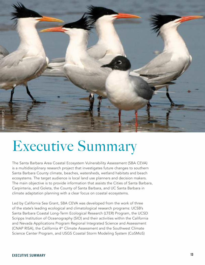
Executive SummaryThe Santa Barbara Area Coastal Ecosystem Vulnerability Assessment (SBA CEVA) is a multidisciplinary research project that investigates future changes to southern Santa Barbara County climate, beaches, watersheds, wetland habitats and beach ecosystems. The target audience is local land use planners and decision makers. The main objective is to provide information that assists the Cities of Santa Barbara, Carpinteria, and Goleta, the County of Santa Barbara, and UC Santa Barbara in climate adaptation planning with a clear focus on coastal ecosystems.
Led by California Sea Grant, SBA CEVA was developed from the work of three of the state’s leading ecological and climatological research programs: UCSB’s Santa Barbara Coastal Long-Term Ecological Research (LTER) Program, the UCSD Scripps Institution of Oceanography (SIO) and their activities within the California and Nevada Applications Program Regional Integrated Science and Assessment (CNAP RISA), the California 4th Climate Assessment and the Southwest Climate Science Center Program, and USGS Coastal Storm Modeling System (CoSMoS)
Callie B
owd
ish
14 SBA CEVA REPORT 2017
and accompanying coastal change monitoring program. Watershed models were developed by researchers at Northeastern University in collaboration with the Santa Barbara Coastal LTER.
CLIMATE CHANGE PROJECTIONS (CAYAN AND IACOBELLIS)
T E M P E R A T U R E A N D P R E C I P I T A T I O N
Projections of temperature and precipitation for the Santa Barbara County region were acquired from statistically downscaled output from 10 global climate models (GCMs) that were selected from models used in the most recent IPCC assessment. Downscaled daily minimum temperature, daily maximum temperature, and daily precipitation from these models covering the 1950−2100 period and using two emission scenarios RCP 4.5 (reduced emissions scenario) and RCP 8.5 (business as usual) were analyzed.
GCMs are powerful tools used to project future climate patterns but have relatively coarse horizontal resolution of 100 km or more. Because the Santa Barbara County region is highly diverse with strong spatial variability (including coastal wetlands, mountains, and inland valleys), the GCM temperature and precipitation output was downscaled to a horizontal resolution of ~6 km (3.73 miles) using the state-of-the-art Localized Constructed Analogs (LOCA) technique.
The downscaled temperature and precipitation from each of the 10 GCMs was averaged over the 1985−2014 historical period as well as three 20-year future periods: 2020−2039, 2040−2059, and 2080−2099. Ensemble means (median used for precipitation) were calculated for each period from the mean period values of the ten models. In addition to daily temperature and precipitation, two derived quantities also were examined: number of extreme hot (equal or exceeding ~88.4 °F for grid cell containing city of Santa Barbara) days and number of wet (equal or exceeding >0.25”) days.
The results for Santa Barbara County are similar to those found elsewhere in southern California from the same downscaled climate models and from other previous studies. Increasing temperature values are projected throughout Santa Barbara County by all models with the RCP 8.5 emission scenario producing larger temperature increases compared to RCP 4.5 emission scenario. Projected average temperature increases with RCP 8.5 scenario are about 1.5°F by year 2030, about 3°F by year 2050 and up to 6-7°F at the end of the century. The projected number of extreme hot days increases significantly throughout the 21st century with largest increases in inland and mountain regions of east Santa Barbara County. Relative to 3-4 extreme hot days per year during the historical period, the projections indicate an increase in the number of extreme hot days per year to 6-10 days by 2030, 9-18 days by 2050, and 23-43 days by 2090 under emission scenario RCP 8.5.

15EXECUTIVE SUMMARY
No consistent trends in annual precipitation are found among the 10 downscaled model projections for the Santa Barbara County region. A majority of models, however, project i) an increase in the variability of annual precipitation; ii) fewer but more intense storms, leading to a decrease in the number of wet days per year and an increase in the number of days with extreme precipitation; and iii) a shortening of the wet season and longer dry spells.
S E A L E V E L R I S E
Projections of hourly sea level over the 21st century along the Santa Barbara County coastline also were constructed. Short-term fluctuations in local sea level were modeled using astronomical tides, variations of wind and atmospheric pressure and effects associated with naturally occurring climate patterns including El Niño and anomalous sea surface temperature along the California Coast, using data from eight of the GCMs (two GCMs did not archive daily wind) with emission scenarios RCP 4.5 and RCP 8.5. Longer-term changes in sea level caused primarily by warming oceans and melting of land-based ice were represented by three scenarios (low, mid, and high range) of sea level rise (SLR) along the California coast from the (2012) National Research Council West Coast sea level rise report.
Under the mid-range SLR scenario and RCP 8.5 emission scenario, sea level heights are projected to increase about 20 cm by 2030, which amounts to the total SLR estimated to have occurred along the Southern California coast during the last 100 years. The mid-range scenario has continuing SLR throughout the 21st century, with 30 cm (~1 ft) by 2050, and 100 cm by the end of the century. The frequency and duration of extreme sea level events are projected to increase significantly, in accord with the steady increase in Mean Sea Level under the SLR regime. These high sea level events are almost always associated with strong low-pressure storm systems with high wind speeds. They have the greatest magnitude when they coincide with high tides and impacts are greatest when they are accompanied by large waves and high runup, often leading to damaging conditions along the shoreline.
Such conditions occurred during the severe winter storm of March 2014 when sea level heights along the Santa Barbara coastline reached 1.24 meters (~4 ft) above Mean Sea Level and surface pressure was about 13 mb below normal. During the 1950−1999 period, the model results produced this combination of sea level height and low pressure once every five years with a usual duration of about two hours. Using the mid-range SLR scenario and business as usual (RCP 8.5) emission scenario, the model projections indicate that by 2090 these conditions occur twice a year with each occurrence lasting about four hours. Adding to events having this extreme combination of high sea level and intense storms, the occurrence of high sea levels (with and without strong storms) increases greatly through the 21st century. Under the mid-range sea level rise scenario, the number of hours of sea levels over the historical 99.99th percentile (one hour in 14 months) level of 1.35 m is projected to increase to roughly 100 hours per year by 2050 and to over 600 hours per year by 2100.

16 SBA CEVA REPORT 2017
WATERSHED RUNOFF (MELACK AND BEIGHLEY)
Information about the impacts of future climate conditions on stream discharge was developed using climate hindcasts and forecasts from an ensemble of global climate models, downscaling modeling results to represent locally relevant precipitation and temperatures, and a hydrologic model, calibrated for local watershed characteristics, to simulate past and future stream discharge. This study of watersheds in coastal Santa Barbara County builds on established methods and past hydrologic studies focused on this region. Findings are intended to provide land use planners and coastal decision makers, including policy makers and water resource managers, with quantitative insights on how future stream discharges compare to current conditions.
In this study, a hydrologic model uses the Scripps downscaled precipitation and temperature data from 10 climate models and two climate scenarios (RCP 4.5–reduced emissions, and 8.5–emissions at current levels) to simulate stream discharge and assess potential impacts of future climate conditions on runoff via streams. Results are provided for selected watersheds in terms of relative change in hydrologic quantities for 2006–2061 and 2045–2100, as compared to a historical period from 1950–2005. Although the model ensemble provides relatively large ranges for almost all hydrologic measures, the median value from the ensemble is the primary metric used to assess likely changes in hydrologic response under future climate conditions. Results of climate models indicate that annual precipitation remains relatively unchanged, but the number of dry days increases and the number of large rainfall events increases. In addition to changes in rainfall events, the rainy seasons start later, end sooner and are generally shorter. The shorter season combined with more large rainfall events leads to more runoff (because of wetter initial conditions) and larger peak discharges (resulting from large rainfall events on wetter soils). The larger annual peaks lead to changes in flood frequency distributions (including increases in 100-yr flood discharges). Overall, results for the higher emission scenario (RCP 8.5) show similar direction of changes as compared to RCP 4.5, but the magnitudes of changes tend to be larger.
The key findings from the watershed runoff study are:
• Change in annual precipitation averaged over coastal watersheds is small.
• The number and magnitude of larger rainfall events increases.
• Annual runoff and annual peak discharge increases.
• Changes in year-to-year variability and an increase in annual peak discharge alter watershed flood frequency distributions.
• Specific discharges (e.g., 100-yr floods) are projected to increase even more than high extreme annual peak discharges.
The emission scenarios result in similar direction of change, with the higher emission scenario (RCP 8.5) generally resulting in larger changes suggesting that, if emissions
17EXECUTIVE SUMMARY
are higher, potential hydrologic changes could be even larger.
With more intense storms projected to occur as the climate changes, the frequency and magnitude of large sediment fluxes are likely to increase. As a consequence, sediment deposition in coastal wetlands and inputs to local beaches are likely to increase. Furthermore, wildfires are common in the Santa Barbara area, and incineration of vegetation can exacerbate erosion and sediment fluxes, especially during large runoff events. Projections of shorter wet seasons and longer droughts will further exaggerate wildfires and their ecosystem impacts.
COASTAL HAZARDS AND SHORELINE CHANGE (BARNARD)
To assess the exposure of Santa Barbara-area ecosystems to coastal hazards associated with climate change, the Coastal Storm Modeling System (CoSMoS) was applied across the region. CoSMoS is a dynamic modeling approach that allows detailed predictions of coastal flooding due to both future sea level rise and storms integrated with long-term coastal evolution (i.e., beach changes and cliff/bluff retreat) over large geographic areas (100s of kilometers). All the relevant physics of coastal storms (e.g., tides, waves and storm surge) were modeled then scaled down to local, 2 meter-scale (6.6 foot-scale) flood projections for use in community-level coastal planning and decision-making. Rather than relying on historic storm records, wind and pressure from global climate models are used to simulate coastal storms under changing climatic conditions during the 21st century. For locally generated seas and surge within the Santa Barbara Channel, we utilized the downscaled wind and pressure fields provided by the Scripps climate team. Further, the modeling resolution was refined in areas of noted societal interest and/or complexity, including Carpinteria (Salt Marsh), Santa Barbara Harbor and Goleta, including Goleta Slough and Devereux Slough, particularly to feed directly into the more detailed ecosystem vulnerability assessments provided by other investigators within this project.
CoSMoS produced coastal flooding projections of multiple storm scenarios (daily conditions, annual storm, 20-year and 100-year return intervals) are provided under a suite of sea level rise scenarios ranging from 0–2 meters (0–6.6 ft), along with an extreme 5-meter (16-ft) scenario. This allows users to manage and meet their own planning horizons and specify degrees of risk tolerance. For each of the 40 sea level rise and storm scenarios, products include: flood extent, depth, duration, elevation and uncertainty based on sustained flooding projections; maximum wave run-up locations; maximum wave height and current speed; and detailed population demographics and economic exposure.
Long-term shoreline change and cliff retreat projections are provided, including uncertainty, using state-of-the-art approaches for each of the 10 sea level rise scenarios. In addition, multiple management scenarios are provided for each of these long-term projections of coastal change, where historical rates of beach nourishment are assumed to continue into the future (or not) and/or where no erosion beyond existing urban infrastructure (or not) was assumed, i.e., “hold the line.” For the
18 SBA CEVA REPORT 2017
integration of coastal change with the flooding projections, it was assumed no further nourishment will occur but that local communities will “hold the line” at the current urban interface.
CoSMoS results indicate serious concerns in the Santa Barbara region over the coming decades. The most vulnerable regions for future flooding across the region include Carpinteria, Santa Barbara Harbor/East Beach neighborhood, Goleta Slough/Santa Barbara Airport, Devereux Slough, and Gaviota State Park. Several of these locations, such as Santa Barbara Airport and Carpinteria, are already vulnerable to coastal flooding from a major storm at present, while the vulnerability of other locations (e.g., East Beach) doesn’t ramp up until later in the century.
Many beaches will narrow considerably and as many as two-thirds will be completely lost over the next century across the region. The further narrowing and/or loss of future beaches (and the ecosystems supported by those beaches) will primarily result from accumulating SLR combined with a lack of ample sediment in the system, which together will continue to drive the landward erosion of beaches, effectively drowning them between the rising ocean and the backing cliffs and/or urban hardscape. The beaches along the UC Santa Barbara shoreline, for example, were almost completely devoid of dry sand at high tide following the El Niño of 2015–2016 through the publication of this study in spring 2017, which both stresses existing sandy beach ecosystems and leaves the cliffs more vulnerable to wave attack, further placing cliff-top ecosystems at risk.
All the model results can be downloaded at USGS Science Base, and viewed interactively and downloaded on the Our Coast, Our Future website, along with the socioeconomic impacts on the Hazard Exposure Reporting and Analytics (HERA) website.
ESTUARIES (PAGE)
Estuarine wetlands of Santa Barbara County are vulnerable to the effects of sea level rise (SLR), which will change the area and distribution of habitats and ecosystem functioning. The effects of SLR were modeled for the fully tidal Carpinteria Salt Marsh, where habitats are closely tied to inundation regime. The effects of SLR were modeled according to NRC 2012 scenarios using LiDAR data corrected for discrepancies imposed by thick vegetation, and geo-referenced multi-spectral aerial imagery and vegetation classification algorithms. Vegetated salt marsh will convert to mudflat over time with rising sea level, but estimates regarding changes by the end of the century range from little change in mudflat (from 9-10% of habitat) under the minimum SLR scenario with 4 mm per year accretion of the marsh surface to >80% of habitat under the maximum SLR scenario assuming no accretion. Changes in inlet dynamics that affect tidal exchange and in fluvial inputs could affect the response of the ecosystem to SLR.
Although little net change in the overall area of vegetated marsh is predicted up

19EXECUTIVE SUMMARY
to about 20 cm of SLR, modeling revealed that the high salt marsh and transition habitats are the most vulnerable to rising water levels, continuously declining in area and evolving into mid marsh habitat unless there are opportunities for these habitats to transgress into upland. However, available upland habitat to accommodate SLR is limited in Carpinteria Salt Marsh, which is surrounded by residential and commercial development and infrastructure (roads, railroad tracks). The only remaining undeveloped area for potential wetland migration connected to the marsh via storm drains under the freeway, is the agricultural land above the eastern end of the marsh.
If high salt marsh and transitional habitats are lost, it is expected that there will be a loss of biodiversity, including regionally rare, threatened and endangered plants. Fourteen of 16 plant species of conservation concern reported from Carpinteria Salt Marsh are found in the high marsh and transition habitat, including Salt Marsh Birds-Beak, Coulter’s Goldfields, and the Ventura marsh milkvetch, which has been planted in the wetland as part of a recovery plan for the species. In addition there would be a loss of foraging and nesting habitat for the endangered Belding’s Savannah Sparrow, and nursery habitat for marsh insects, such as the Wandering Skipper Butterfly. Our study also indicates a threshold of ~30 cm when an abrupt increase in the proportion of mudflat habitat is expected. Mudflat and subtidal habitats are the least vulnerable to the adverse impacts of SLR. The increase in area of mudflat could benefit shorebirds that use this habitat for foraging and loafing.
Two other estuarine wetlands discussed in this study, Devereux and Goleta Sloughs, are open intermittently to tidal exchange. Devereux Slough has historically been non-tidal for most of the year, with tidal exchange blocked by a sand berm at the inlet. Plant distributions are shifted higher in Devereux than Carpinteria Salt Marsh due to the formation of a lagoon during the winter that submerges lower elevations. Ecological Science Associates (ESA) modeling of lagoon water levels with SLR suggests that plant distributions may shift even higher in Devereux, depending on rates of accretion of the slough surface. Less surrounding infrastructure and the incorporation of SLR into restoration activities provides opportunity for the transgression of marsh vegetation inland at Devereux in response to SLR.
The effects of SLR on Goleta Slough were first modeled by ESA assuming open inlet conditions and generally conform to our results for Carpinteria Salt Marsh (i.e., conversion of some vegetated marsh to mudflat by 2100). Goleta Slough has recently (2013) been allowed to close and may develop habitat characteristics more similar to Devereux Slough as water ponded behind the beach berm could cause the conversion of vegetated marsh to mudflat at lower elevations and the transgression of marsh vegetation into transition and upland habitat. However, this modeling suggested that eventually the greater tidal prism in Goleta Slough may allow the inlet to remain open longer following breaching events and that the wetland could become largely tidal with 0.9 m (3 ft) of SLR. In Goleta Slough, the availability of convertible upland habitats is limited by existing infrastructure, including the Santa Barbara Airport.

20 SBA CEVA REPORT 2017
There is considerable uncertainty regarding the timing of ecosystem changes associated with SLR that will depend on future rates of SLR, accretion of the marsh surface, and estuarine tidal dynamics. The uncertainty regarding timing of SLR creates challenges for land use planners since any implemented adaptation strategy to accommodate future SLR should not adversely affect the existing functioning of the estuary (e.g., by increasing sediment delivery, introduction of infrastructure).
BEACHES (DUGAN)
The vulnerability of beach ecosystems to pressures from climate change, especially sea level rise and storminess, was evaluated. We integrated the results of CoSMoS (version 3.0) with the elevations of key intertidal zones to generate predictions of the ecological responses of beach ecosystems to sea level rise. We focused on measuring and modeling the ecologically important upper intertidal zones of beach ecosystems that appear to be most vulnerable to storm erosion and sea level change. Located closest to the landward boundaries of the beaches, these zones are ecologically vital and critically important to biodiversity and ecosystem function. CoSMoS runup outputs for ambient and 1-year storm conditions were used as a proxy for the elevation of the lower boundary of upper beach zones under future sea level conditions. Our study included seven beaches representing a range of beach types on the Santa Barbara south coast, Sands/Ellwood, West Isla Vista, East Campus, Arroyo Burro, East Beach, Santa Claus Lane and Carpinteria City/State Beach.
Sandy beaches compose the majority of open coast shoreline of the south coast of Santa Barbara County. The majority of these beaches (78%) are bluff-backed with little scope for shoreline retreat. Dune-backed beaches with more scope for retreat are scarce in the study area with <3% remaining undeveloped. About 24% of the beaches are developed and managed, including armored and groomed beaches. Sandy beach ecosystems of our study area represent a range of conditions from relatively undeveloped to highly urbanized and managed. The unmanaged and undeveloped beach ecosystems of southern Santa Barbara County currently support remarkably rich intertidal communities that are prey for birds and fish and provide ecosystem function and services. In contrast, the groomed beaches and many of the armored beaches in the study area presently support impoverished intertidal food webs, particularly in the wrack-dependent upper intertidal zone.
The majority of beaches in the study area were projected to decline in overall width with increasing SLR. However, the loss of beach width will not be evenly distributed across intertidal zones. Upper beach zones are projected to experience the greatest declines in width and losses with SLR. These vulnerable upper beach zones are already scarce and/or ephemeral for many beaches in the study region. For all the study beaches, model results projected significant declines (average >70%, range 51-98%) in the widths of upper intertidal zones with 50 cm of SLR, which will occur by 2070 or earlier if GHG emissions continue “business as usual.”
The projected responses of beach ecosystems to sea level rise were strongly affected
21EXECUTIVE SUMMARY
by the potential for the shoreline to retreat. This means the type of landward boundary and the degree of human alterations in the form of coastal armoring and development are important factors in considering the vulnerability of beach ecosystems to climate change.
A rapid loss of upper beach and mid beach zones with increasing SLR was projected for the bluff-backed beaches with <15% of this critical upper beach zone estimated to remain with 50 cm SLR at the study beaches (West Isla Vista, East Campus, Arroyo Burro). The limited scope for retreat of bluff-backed beaches restricts their ability to adjust and makes them highly vulnerable to SLR. With projected climate change and SLR, upper beach zones will become increasingly rare and vanish from much of the bluff-backed dominated Santa Barbara coast, resulting in major declines in biodiversity and ecosystem function. Beaches with shoreline armoring that limits potential migration of the shoreline were projected to have the most rapid loss of upper and mid beach zones with SLR (~99% for upper zone at Santa Claus Lane).
Dune-backed beaches at Sands/Ellwood were projected to have the greatest resilience to increasing SLR for upper and mid intertidal zones, maintaining a narrow zone of upper beach (9%) even with 200 cm SLR. However even the dune-backed beach lost >60% of the width of the upper beach zone with 50 cm of SLR. The dune-backed section of Carpinteria State Beach also maintained some upper beach zone width at 50 cm SLR.
East Beach, which has an artificially wide upper intertidal zone associated with beach grooming and filling, was projected to have some resilience to SLR but still lost >50% of upper zone width with 50 cm SLR. The current management of East Beach and other groomed urban beaches has resulted in impoverished intertidal biota, a lack of resilient coastal dunes and reduced ecological function. However, this model result suggests exploring opportunities to restore biodiversity, coastal dunes and ecosystem function of these degraded but relatively wide beaches could potentially enhance the conservation of vulnerable beach ecosystems under SLR in the study area and elsewhere.
E L N I Ñ O A N D T I P P I N G P O I N T S
The 2015–2016 El Niño provided a window into future climate change impacts. Winter wave energy 50% above normal and water levels 5-6” above normal eroded beaches in the region beyond historical extremes. The result was loss of intertidal habitat, affecting the diversity and functioning of beach ecosystems, and stressed vegetated salt marsh that, with future long-term sea level rise of this magnitude, will convert to mudflat habitat. El Niño events, along with short period North Pacific storm extremes, are projected to continue with climate warming and likely will cause the heaviest coastal and terrestrial impacts. The major tipping point where exposure of beaches and wetlands to coastal hazards increases dramatically is 0.5-1.0 m (~20-40”) of sea level rise and is projected to occur in the mid-21st century. The structure and function of beach and wetland ecosystems will be severely impacted even earlier (at ~0.3 m (12”) of sea level rise).
22 SBA CEVA REPORT 2017
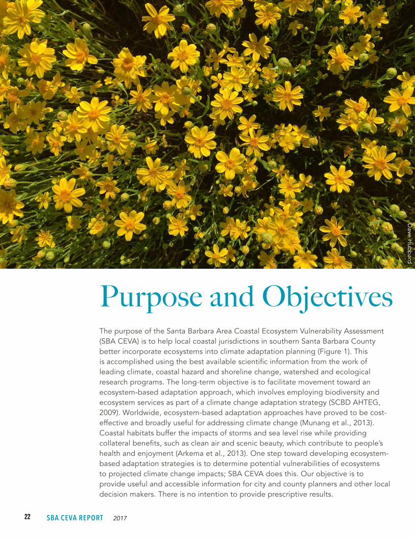
Purpose and ObjectivesThe purpose of the Santa Barbara Area Coastal Ecosystem Vulnerability Assessment (SBA CEVA) is to help local coastal jurisdictions in southern Santa Barbara County better incorporate ecosystems into climate adaptation planning (Figure 1). This is accomplished using the best available scientific information from the work of leading climate, coastal hazard and shoreline change, watershed and ecological research programs. The long-term objective is to facilitate movement toward an ecosystem-based adaptation approach, which involves employing biodiversity and ecosystem services as part of a climate change adaptation strategy (SCBD AHTEG, 2009). Worldwide, ecosystem-based adaptation approaches have proved to be cost-effective and broadly useful for addressing climate change (Munang et al., 2013). Coastal habitats buffer the impacts of storms and sea level rise while providing collateral benefits, such as clean air and scenic beauty, which contribute to people’s health and enjoyment (Arkema et al., 2013). One step toward developing ecosystem-based adaptation strategies is to determine potential vulnerabilities of ecosystems to projected climate change impacts; SBA CEVA does this. Our objective is to provide useful and accessible information for city and county planners and other local decision makers. There is no intention to provide prescriptive results.
Dave H
ubb
ard
23INTRODUCTION
Ecosystems and the services they provide are being impacted by climate change in California (Barry, 1995; Moritz et al., 2008; Bentz et al., 2010) and on every continent and ocean on Earth (Hughes, 2000; Steneck, 2002; Hoegh-Guldberg and Bruno, 2010; IPCC, 2014). Local governments can play an important role in reducing these impacts.
In the Santa Barbara area, local land use decisions are key in determining the fate of coastal ecosystems. Because approximately half the land in California is owned privately, local governments regulate general land use and development activity for a tremendous amount of the natural environment. Here, it is particularly important for local governments to have good information about potential climate change impacts to coastal ecosystems. Adaptation needs to take place at the local level (Roberts et al., 2012) and ecological information needs to be an integral component.
Coastal ecosystem protection is fundamental to California coastal legislation. The 1976 California Coastal Act prioritizes protection of the ecological balance of the coastal zone (CCA Sections 3001 and 3001.5). The Legislature’s findings state, “That the permanent protection of the state’s natural and scenic resources is a paramount concern to present and future residents of the state and nation…” and “That to promote the public safety, health, and welfare, and to protect public and private property, wildlife, marine fisheries, and other ocean resources, and the natural environment, it is necessary to protect the ecological balance of the coastal zone and prevent its deterioration and destruction.” Wetlands and dunes are specifically identified as “environmentally sensitive habitat areas” (ESHA) that “shall be protected against disruption of habitat values”and “development adjacent to ESHA must be designed to prevent impacts that would degrade those areas” (CCA Section 30240). Implementing this legislation falls to local governments who carry out the priorities of the Coastal Act and have authority to regulate land use in the coastal zone.
A survey of California coastal professionals, including city/county planners, indicated ecosystems as a key area of concern for local-level climate change adaptation (Finzi et al., 2011). Loss of wetlands and endangered species were identified as the two top management challenges related to climate adaptation with loss of habitat and native/protected species in the top five. But relatively few climate vulnerability assessments of natural areas have been performed. Most ecosystem vulnerability assessments have focused on particular natural areas (for example, Great Barrier Reef, Chesapeake Bay, Delaware Bay, Cook Inlet) (Grannis, 2011; Swanston et al., 2011; Glick et al., 2012; Kreeger, 2010; Johnson and Marshall, 2007) or species (Gardali et al., 2012; Nur et al., 2012), while some have addressed states (AFWA, 2011), regions (Naumann et al., 2011; NWF, 2007) and nations (Natural England and RSPB, 2014). SBA CEVA may be the first multidisciplinary research project specifically aimed at informing local jurisdictions about ecosystem impacts.
1. Introduction

24 SBA CEVA REPORT 2017
S A N T A B A R B A R A A R E A V U L N E R A B I L I T Y A S S E S S M E N T S
All Santa Barbara area jurisdictions in the study area are planning for climate change. The City of Santa Barbara, the City of Goleta, and County of Santa Barbara have initiated and/or participated in climate/sea level rise vulnerability studies (Griggs and Russel, 2012; City of Goleta, 2015; ESA, 2015c). Climate action plans (CAPs) have been adopted by the Cities of Santa Barbara (2012) and Goleta (2014). The County of Santa Barbara is in the process of using information from its sea level rise vulnerability assessment to craft relevant Coastal Land Use Plan (LUP) policies. The City of Santa Barbara is updating their Coastal Land Use Plan and preparing a Sea Level Rise Adaptation Plan, which will be informed by SBA CEVA. The City of Carpinteria also is in the process of incorporating a sea level rise vulnerability assessment and adaptation plans in their Local Coastal Program (LCP) update, which will be informed by SBA CEVA. Vulnerability assessments provide useful information about the built and physical environment, such as impacts to infrastructure, change in the width of the beach and/or the change in wetland area (physical change). They, generally, do not provide detailed information about changes to natural communities and habitats (ecosystem-level change). While this is not surprising since natural systems are complex and difficult to evaluate, it leaves an important gap in informing planning efforts and coastal policies. This report represents an effort to help fill this gap.
1.1 BACKGROUND
C L I M A T E C H A N G E
The Santa Barbara area and all natural and human systems throughout the world are impacted by climate change (IPCC, 2014). These mostly adverse effects are projected to increase in severity (Mooney et al., 2009; Runting et al., 2017). While efforts are being made to address climate change, global emissions of greenhouse gases (GHG) continue to rise. For example, GHG emissions increased 1.3% per year between 1970 and 2000, 2.2% per year from 2000 to 2010, and 3% between 2010 and 2011. In total, greenhouse gas emissions roughly doubled between 1970 and 2010 (IPCC, 2014). Even if emissions stopped today, greenhouse gases already in the atmosphere would continue to affect global climate many decades into the future. For example, CO2, which comprises over 70% of total GHG emissions, stays in the atmosphere 30-95 years (Jacobson, 2005.) While new policy decisions and consequent actions are critical to determining the severity of future impacts, we can be certain our natural and built environments will change substantially. Land use planners face a new paradigm: planning for a future with a changing climate.
The Earth’s surface temperature has risen about 2°F since record keeping began in the late 19th century. Most of that increase occurred since 1970 with the most recent decade as the hottest. Indeed, the 10 hottest years on record have occurred since 1998, while the 20 coldest occurred before 1930. NOAA and NASA reported 2016 as the hottest year ever recorded globally and the third year in a row that global average surface temperatures hit new records. The first three months of 2017 were
25INTRODUCTION
the second warmest January-March on record, 4.7°F above the century average, with the record set in 2012 (NOAA, 2017).
The 3rd National Climate Assessment indicated the Southwestern U.S. is one of the regions most impacted by climate change in North America (Jardine et al., 2013). Here, average annual temperature and average temperatures for all seasons are increasing. The number of cold snaps along with the length of the freeze-free season is decreasing. Droughts are becoming more severe and more frequent with summer heat waves continuing to increase in temperature and duration. Spring is coming earlier (Cayan et al., 2001). Precipitation is decreasing. River flow and soil moisture continue to decline. Mountain snowpack is decreasing and snowmelt is happening earlier with continued reductions in late winter snow pack (Mote et al., 2005).
S E A L E V E L I S R I S I N G
Sea level is rising as glaciers and ice sheets melt and the Earth’s warming oceans expand. Globally, since 1993 sea levels have increased by about 3 mm (0.1”) per year; by 2100 projections are for 0.28-0.89 m (approximately 1-3 ft) (IPCC 5th Assessment Working Group, 2013). Sea level, however, does not rise uniformly throughout the world. Interestingly, in the western tropical Pacific sea level increased by over 1 cm/year (.4”) during the last 25 years (Merrifield et al., 2012), while the
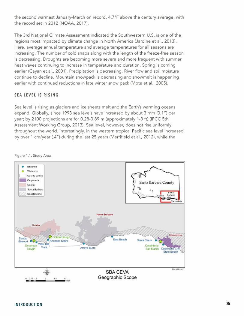
Figure 1.1. Study Area
26 SBA CEVA REPORT 2017
West Coast of the U.S. enjoyed almost no increase (Bromirski et al., 2011). This, however, is changing. Recent research indicates a shift occurred in wind patterns associated with the Pacific Decadal Oscillation (PDO). Sea level on the U.S. West Coast is now rising more rapidly than the global mean (Hamlington et al., 2016). This will continue, potentially sharply (Bromirski et al., 2011), leading to substantially higher sea level on the California coast (Hamlington et al., 2016).
C L I M A T E C H A N G E I S A L R E A D Y I M P A C T I N G E C O S Y S T E M S
Ecosystems respond to climate change in a variety of ways, including changes in location and/or diversity of species, increased incidence of disease and decreased productivity (Harley et al., 2006; Hoegh-Guldberg and Bruno, 2010). Worldwide, species are increasingly at risk of extinction (Thomas et al., 2004; Pounds et al., 2006; Urban, 2015). In Yosemite National Park, increased temperatures over the last 100 years have resulted in small-mammal
species moving up to a half kilometer upward in elevation (Moritz et al., 2008). Warming summer and winter temperatures are allowing bark beetles to destroy millions of hectares of forest in California and across the U.S. (Bentz et al., 2010). California rocky intertidal species have shifted northward, consistent with climate warming predictions (Barry, 1995).
California has experienced ocean warming events that may provide previews of future conditions. In 2014–2015, a warm water “blob” extending from the Gulf of Alaska to Baja California, Mexico, formed in the coastal ocean (~3°C above 1982–2014 levels) from the Gulf of Alaska to Baja California, Mexico. This sea surface temperature anomaly resulted in reduction in coastal upwelling and productivity south of Point Conception, changes in fish (sardine and anchovy) and zooplankton abundance, and intrusions of warm-water species (Leising et al., 2015). The recent 2016 El Niño conditions caused extreme coastal ocean warming, strong wave activity, and raised sea level. While impacts to local kelp forests were minor (Reed et al., 2016), other Santa Barbara area ecosystems were affected (Box 4, p. 122).
P R O J E C T S E T T I N G / S T U D Y A R E A
The SB CEVA study area is located in the southeast corner of Santa Barbara County in Southern California on the West Coast of the United States (Figure 1.1). The region has significant geographical diversity that extends from steep watersheds down to an expansive array of sandy beaches, which comprise most of the shoreline, and
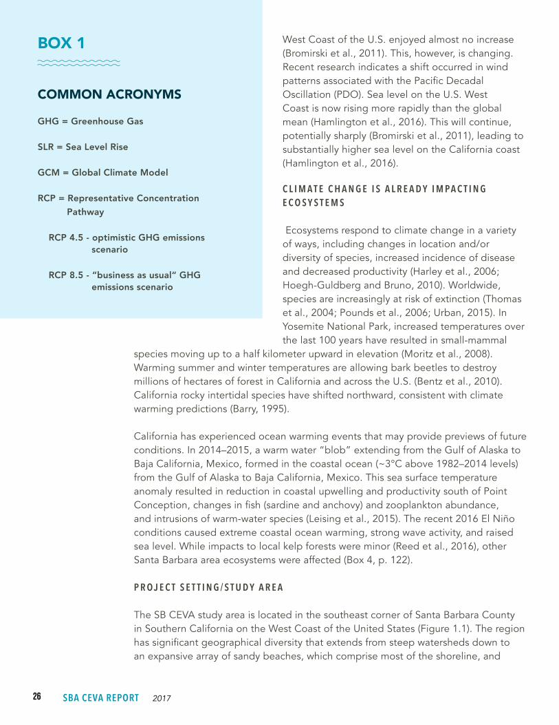
BOX 1
COMMON ACRONYMS
GHG = Greenhouse Gas
SLR = Sea Level Rise
GCM = Global Climate Model
RCP = Representative ConcentrationPathway
RCP 4.5 - optimistic GHG emissionsscenario
RCP 8.5 - “business as usual “ GHGemissions scenario

27INTRODUCTION
important but fragmented coastal wetlands. It includes the cities of Goleta, Santa Barbara, and Carpinteria and the University of California Santa Barbara campus. Coastal ecosystems within cities and county limits include: sandy beaches, coastal dunes, coastal strand zones, sloughs, lagoons, salt marshes, rocky intertidal reefs, and creeks and riparian areas.
S A N T A B A R B A R A C O U N T Y A N D C I T I E S O F G O L E T A , S A N T A B A R B A R A A N D C A R P I N T E R I A
The County of Santa Barbara extends from Point Conception to just east of the City of Carpinteria, straddling the southern and central California coast. It has a land area of 2,735 square miles and a population of approximately 424,000. The southeastern corner of the County includes the unincorporated communities of Summerland, Montecito, Hope Ranch and Isla Vista. The County includes one of Southern California’s least developed coastal areas, the Gaviota Coast, which includes approximately 45 miles of narrow beaches backed by coastal bluffs. Within the county is Goleta Beach County Park and Goleta Slough.
The City of Santa Barbara is located approximately 100 miles north of Los Angeles with a land area of 21.75 square miles. It is on an east-west trending coastal plain with the Pacific Ocean to the south and the Santa Ynez Mountains to the north. About half of the city of Santa Barbara’s 5.75-mile shoreline is maintained beaches, and about half of the shoreline is narrow or intertidal beaches backed by eroding cliffs of up to 60 feet in height. Approximately eight miles west of the city’s main area (connected to the city offshore), a separate 952 acres of low-lying land comprises the city airport, adjacent industrial land, and most of the Goleta Slough. The city, which is home to approximately 90,000 residents of diverse ethnicity, is largely built out with about 22% open space including beaches, parks, preserves, and recreational facilities, and a growth rate of less than 1% per year.
The City of Goleta lies 10 miles west of the city of Santa Barbara with a land area of 7.9 square miles and population of approximately 30,000. Goleta also is located on the narrow, east-west trending coastal shelf nestled between the Pacific Ocean and the Santa Ynez Mountains. Goleta has approximately 10% open space, including Monarch Butterfly habitat and vernal pools. The city’s coastline encompasses a long stretch of beaches, eroding coastal cliffs and two coastal wetlands. Goleta Slough and Devereux Slough, a small upland portion of Goleta Slough and their watersheds are within the city limits.
The City of Carpinteria lies 12 miles southeast of Santa Barbara, but is considerably smaller, with a land area of 2.6 square miles and a population of approximately 13,500. It is mostly near sea level and located entirely in the coastal zone. It is surrounded by a rural setting with natural coastal terrain and agricultural land that is part of the County of Santa Barbara. The Carpinteria Bluffs, over 150 acres of a relatively undisturbed coastal open space, consist of native grasslands and scrub areas overlooking rocky intertidal pools and sandy beach areas, with a tideland
28 SBA CEVA REPORT 2017
area of 4.7 square miles. The 230-acre Carpinteria Salt Marsh is one of Southern California’s larger natural coastal wetlands. One secluded Carpinteria sandy beach hosts one of the last harbor seal rookeries on the mainland coast of Southern California.
N A T U R A L E N V I R O N M E N T A N D E C O S Y S T E M S E R V I C E S
The Santa Barbara area has a unique biogeographic setting that contributes to its exceptional biodiversity both on land and in the ocean. The cold waters of the California Current travel southward down the U.S. West Coast. At Point Conception the coastline “turns” inland extending east-west, forming the western boundary of the Santa Barbara Channel and a major oceanic and biogeographic boundary. In the Santa Barbara Channel the cold, northern waters mix with warmer, nearshore Southern California waters. This transition zone has rich diversity of fauna from Oregonian and Californian biogeographic provinces. The terrestrial environment is part of the large California Floristic Province, a hotspot of plant biodiversity that includes all of coastal California. Examples of rare and endangered plants and animals in the area include: salt marsh bird’s-beak, Belding’s savannah sparrows, Western snowy plovers, and globose dune beetles.
The natural environment is extremely valuable, providing numerous “ecosystem services,” or benefits to humankind. The two focal ecosystems of SBA CEVA–wetlands and sandy beaches–alone, provide: water filtration, regulation of water flow, moderation of climate, reduction of coastal erosion, habitat for numerous species, including endangered plants and animals, and resting, nesting and mating grounds for migratory birds, butterflies, marine mammals and commercially important fishes. Further, the natural world is vital to the character and economy of the Santa Barbara area, contributing open space, aesthetic qualities, recreational opportunities, tourism and spiritual and cultural value.
SBA CEVA projects future changes to the Santa Barbara area’s natural and physical environment. Climate, watershed runoff, and coastal hazards research (Sections 2-4) are included in SBA CEVA because of their important impact on ecosystem condition. The relationship between the SBA CEVA study areas is depicted in Figure 1.2. The focal ecosystems are beaches and wetlands (Sections 5 and 6), although the project results will be useful to future vulnerability assessments of other coastal ecosystems and the built environment.

29INTRODUCTION
Figure 1.2. SBA CEVA Concept Diagram
30 SBA CEVA REPORT 2017
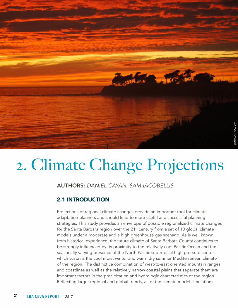
2. Climate Change Projections AUTHORS: DANIEL CAYAN, SAM IACOBELLIS
2.1 INTRODUCTION
Projections of regional climate changes provide an important tool for climate adaptation planners and should lead to more useful and successful planning strategies. This study provides an envelope of possible regionalized climate changes for the Santa Barbara region over the 21st century from a set of 10 global climate models under a moderate and a high greenhouse gas scenario. As is well known from historical experience, the future climate of Santa Barbara County continues to be strongly influenced by its proximity to the relatively cool Pacific Ocean and the seasonally varying presence of the North Pacific subtropical high pressure center, which sustains the cool moist winter and warm dry summer Mediterranean climate of the region. The distinctive combination of west-to-east oriented mountain ranges and coastlines as well as the relatively narrow coastal plains that separate them are important factors in the precipitation and hydrologic characteristics of the region. Reflecting larger regional and global trends, all of the climate model simulations
Aaron H
oward
31CLIMATE CHANGE PROJECTIONS
produce significant warming, and an accompanying set of sea level projections all experience rising ocean levels over the 21st century. Extreme events, including heavy rains, dry spells, heat waves and high sea level episodes are critically important to planning and adaptation, and so daily temperature and precipitation and hourly sea level projections are considered in this assessment.
C L I M A T E O F T H E S A N T A B A R B A R A A R E A
The characteristics of the region’s climate is similar to most of Southern California with warm and relatively dry summers and cool moist winters (Iacobellis et al., 2016). Nearly all of the precipitation occurs during the cool months of October-April from North Pacific extratropical storms, with most freshwater runoff occurring between December and March (Beighley et al., 2005). The northeastward expansion of the North Pacific subtropical high pressure center in spring and summer results in mostly dry conditions, with appreciable precipitation almost entirely lacking during the warmest summer months. This strong Mediterranean precipitation seasonality is an important factor influencing ecosystems throughout the region.
A characteristic of the geography are the Santa Ynez Mountains that run east-west along the southern portion of the county. During winter storms with strong southerly winds, the south-facing slopes of these mountains induce uplift of the moist air that often leads to daily precipitation amounts that may exceed 2”, with occasional extremes that exceed 5”. These precipitation events can significantly impact downstream coastal ecosystems as well as the human population centers along the coastal region of the county.
2.2 METHODS
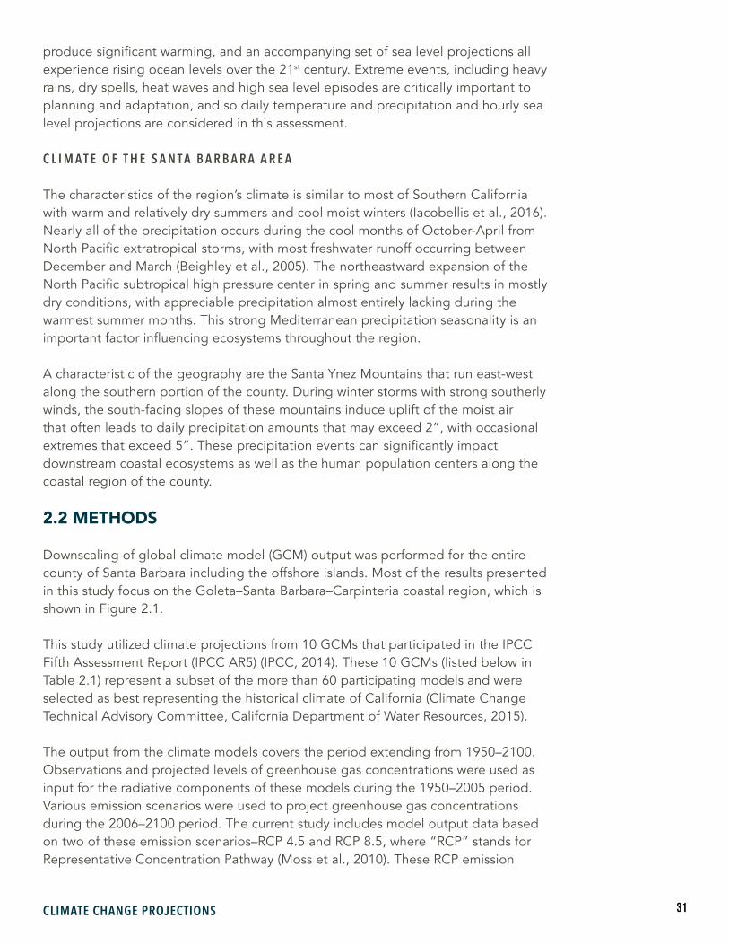
Downscaling of global climate model (GCM) output was performed for the entire county of Santa Barbara including the offshore islands. Most of the results presented in this study focus on the Goleta–Santa Barbara–Carpinteria coastal region, which is shown in Figure 2.1.
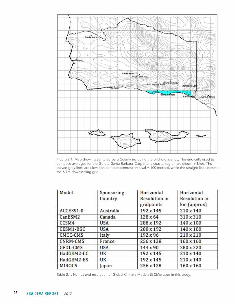
This study utilized climate projections from 10 GCMs that participated in the IPCC Fifth Assessment Report (IPCC AR5) (IPCC, 2014). These 10 GCMs (listed below in Table 2.1) represent a subset of the more than 60 participating models and were selected as best representing the historical climate of California (Climate Change Technical Advisory Committee, California Department of Water Resources, 2015).
The output from the climate models covers the period extending from 1950–2100. Observations and projected levels of greenhouse gas concentrations were used as input for the radiative components of these models during the 1950–2005 period. Various emission scenarios were used to project greenhouse gas concentrations during the 2006–2100 period. The current study includes model output data based on two of these emission scenarios–RCP 4.5 and RCP 8.5, where “RCP” stands for Representative Concentration Pathway (Moss et al., 2010). These RCP emission
32 SBA CEVA REPORT 2017
Figure 2.1. Map showing Santa Barbara County including the offshore islands. The grid cells used to compose averages for the Goleta–Santa Barbara–Carpinteria coastal region are shown in blue. The curved grey lines are elevation contours (contour interval = 100 meters), while the straight lines denote the 6-km downscaling grid.
Table 2.1. Names and resolution of Global Climate Models (GCMs) used in this study.

33CLIMATE CHANGE PROJECTIONS
scenarios were initially implemented for the Intergovernmental Panel on Climate Change (IPCC) 5th Assessment Report and replaced the Special Report on Emissions Scenarios (SRES)-based scenarios used in earlier IPCC assessment reports. RCP 4.5 is a relatively low emissions scenario and is qualitatively similar to the “optimistic” SRES B1 scenario, whereas RCP 8.5 is a relatively high emissions scenario and most similar to the “business as usual” SRES A1 family of scenarios.
C L I M A T E M O D E L I N G
The horizontal resolution of the global climate models is on the order of 100s of km and do not by themselves provide information on fine enough spatial scales to adequately examine the high spatial variability of Santa Barbara County. To provide climate data at fine horizontal resolution, the climate model output was “downscaled” using the Localized Constructed Analogs (LOCA) technique of Pierce et al., (2014). The LOCA method improves on previous methods, including representation of precipitation and temperature extremes. The downscaled data include daily minimum and maximum surface air temperatures and precipitation at ~6-km (1/16th degree) resolution. The LOCA runs were made over the conterminous U.S., southern Canada and Mexico, but for our purposes we will use a subset of these data on a 6-km grid that covers the Santa Barbara region (see Figure 2-1; Note: downscaled temperature and precipitation data in coastal grid cells including both land and water are representative of the land portion). The downscaling procedure was applied to the output from each of the 10 climate models run under both emission scenarios (20 individual model runs).
Figure 2.2. Modeled daily precipitation over Southern California on January 9, 2005 at the original 1° resolution (left panel) and after downscaling to 1/16° resolution using the LOCA downscaling technique (courtesy David Pierce, SIO).
34 SBA CEVA REPORT 2017
An illustrative example of the benefits derived through downscaling is provided in Figure 2.2 that shows modeled daily precipitation over Southern California during a strong storm event on Jan. 9, 2005. The left-hand panel shows the modeled product at 1° x 1° (~100 km) resolution, while the right-hand panel shows the same product at 1/16° x 1/16° (~6 km) resolution after downscaling was applied. The downscaled data resolves regional precipitation features throughout the domain and in particular, the Santa Barbara region.
The GCM output data was downscaled to a 6-km resolution over a domain covering the California-Nevada region. From this, a subset of downscaled data covering Santa Barbara County (including offshore islands) was selected for the current study.
W A T E R L E V E L M O D E L I N G
Deviations from the predicted astronomical tide along the Santa Barbara County coastline are due to both meteorological influences and long-term global sea level rise. Collectively these are referred to as the residual water level.
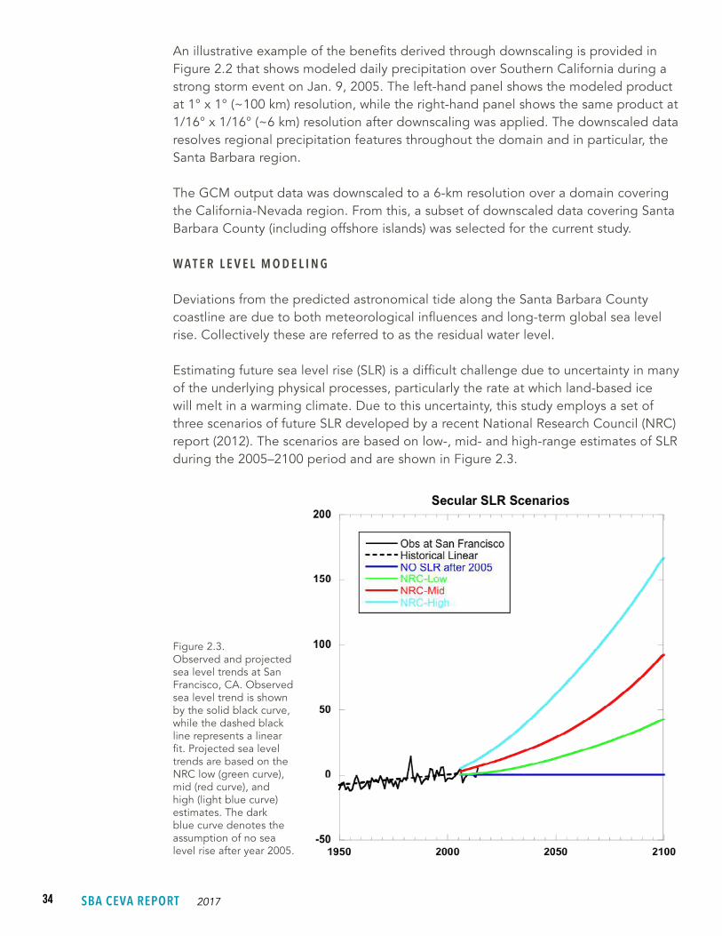
Estimating future sea level rise (SLR) is a difficult challenge due to uncertainty in many of the underlying physical processes, particularly the rate at which land-based ice will melt in a warming climate. Due to this uncertainty, this study employs a set of three scenarios of future SLR developed by a recent National Research Council (NRC) report (2012). The scenarios are based on low-, mid- and high-range estimates of SLR during the 2005–2100 period and are shown in Figure 2.3.
Figure 2.3. Observed and projected sea level trends at San Francisco, CA. Observed sea level trend is shown by the solid black curve, while the dashed black line represents a linear fit. Projected sea level trends are based on the NRC low (green curve), mid (red curve), and high (light blue curve) estimates. The dark blue curve denotes the assumption of no sea level rise after year 2005.
35CLIMATE CHANGE PROJECTIONS
The short period sea level fluctuation (the meteorological component of residual water level) is estimated using a multi-linear regression model constructed with water level observations at Santa Barbara Harbor and historical reanalysis data to specify the necessary forcing meteorological variables. Future values of the meteorological component of residual water level are then projected by applying the regression model with the necessary input for the model derived from output of 8 of the 10 GCMs noted in Table 2.1 (models CCSM4 and CESM1-BGC did not archive all necessary data at the daily time scale and could not be used for the water level modeling component). The reanalysis data products used to construct the regression model have temporal and spatial resolution similar to the climate models.
S E A L E V E L F L U C T U A T I O N R E G R E S S I O N M O D E L D E V E L O P M E N T
Observed hourly residual water levels are determined by subtracting the predicted astronomical tide from the observed water level. A long-term trend is then computed using a linear best-fit through the residual water level values. Daily values of the meteorological component of residual water level are computed by removing the long-term trend from the daily mean residual water level.
Daily mean values of the local surface pressure, local offshore surface wind stresses (tx = east-west; and tY = north-south), local sea surface temperature (SST), and SST in the eastern tropical Pacific Ocean as a measure of El Niño variability (designated as N3.4) from National Centers for Environmental Prediction (NCEP) Reanalysis and the eight GCMs are used as forcing in this study. The time series of each variable was first detrended then anomalized by removing the annual cycle smoothed with a 31-day running mean filter. The annual cycle was removed since the astronomical tides include annual and semi-annual terms. During the development phase of the regression model several additional variables were considered (e.g., Pacific Decadal Oscillation index, geopotential height) as potential forcing, but were not included in the final model due to relatively low significance (magnitude of standardized regression coefficient <0.05) in predicting the meteorological component of residual water level.
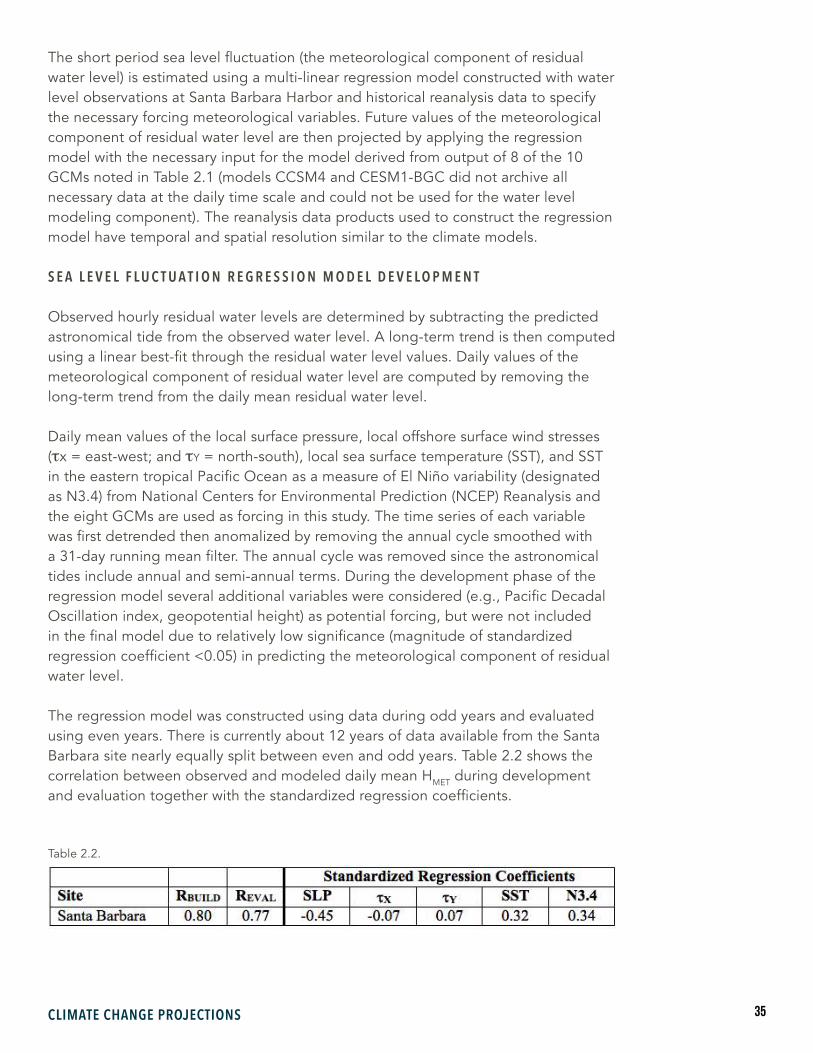
The regression model was constructed using data during odd years and evaluated using even years. There is currently about 12 years of data available from the Santa Barbara site nearly equally split between even and odd years. Table 2.2 shows the correlation between observed and modeled daily mean HMET during development and evaluation together with the standardized regression coefficients.
Table 2.2.
BOX 2
2015–16 EL NIÑO IMPACTS TO THE SANTA BARBARA AREA
E V E R Y E L N I Ñ O I S D I F F E R E N T
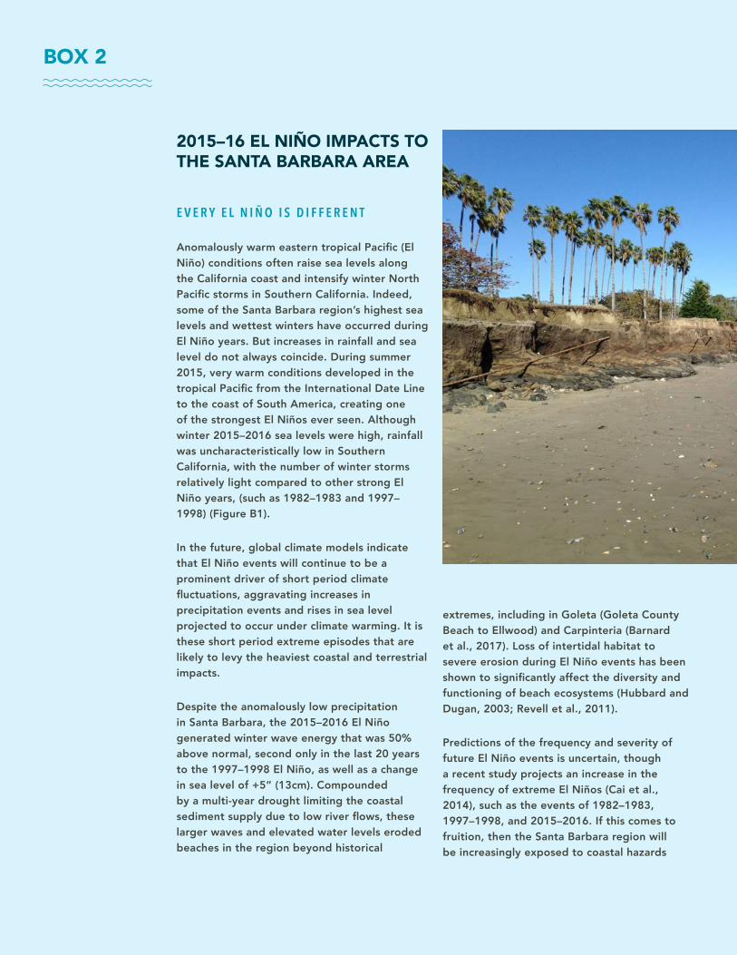
Anomalously warm eastern tropical Pacific (El Niño) conditions often raise sea levels along the California coast and intensify winter North Pacific storms in Southern California. Indeed, some of the Santa Barbara region’s highest sea levels and wettest winters have occurred during El Niño years. But increases in rainfall and sea level do not always coincide. During summer 2015, very warm conditions developed in the tropical Pacific from the International Date Line to the coast of South America, creating one of the strongest El Niños ever seen. Although winter 2015–2016 sea levels were high, rainfall was uncharacteristically low in Southern California, with the number of winter storms relatively light compared to other strong El Niño years, (such as 1982–1983 and 1997–1998) (Figure B1).
In the future, global climate models indicate that El Niño events will continue to be a prominent driver of short period climate fluctuations, aggravating increases in precipitation events and rises in sea level projected to occur under climate warming. It is these short period extreme episodes that are likely to levy the heaviest coastal and terrestrial impacts.
Despite the anomalously low precipitation in Santa Barbara, the 2015–2016 El Niño generated winter wave energy that was 50% above normal, second only in the last 20 years to the 1997–1998 El Niño, as well as a change in sea level of +5” (13cm). Compounded by a multi-year drought limiting the coastal sediment supply due to low river flows, these larger waves and elevated water levels eroded beaches in the region beyond historical
extremes, including in Goleta (Goleta County Beach to Ellwood) and Carpinteria (Barnard et al., 2017). Loss of intertidal habitat to severe erosion during El Niño events has been shown to significantly affect the diversity and functioning of beach ecosystems (Hubbard and Dugan, 2003; Revell et al., 2011).
Predictions of the frequency and severity of future El Niño events is uncertain, though a recent study projects an increase in the frequency of extreme El Niños (Cai et al., 2014), such as the events of 1982–1983, 1997–1998, and 2015–2016. If this comes to fruition, then the Santa Barbara region will be increasingly exposed to coastal hazards

Figure B1. Extreme beach erosion at Goleta County Beach during the 2015–2016 El Niño (Photo: D. Hoover, USGS).
such as severe beach erosion, cliff failures and coastal flooding, which will be exacerbated by accelerating sea level rise. Increased exposure to these coastal hazards combined with SLR will strongly affect the diversity and functioning of beach ecosystems.
A W I N D O W T O F U T U R E E S T U A R I N E E C O S Y S T E M S
The habitat in estuarine wetlands is largely determined by elevation and frequency of saltwater inundation, which is affected by sea level. Small differences in marsh surface elevation separate mudflat, middle, and high marsh habitats. Short-term rises in sea level
of several inches, associated with the 2015 El Niño, increased the frequency of saltwater inundation at lower elevation sites providing a unique opportunity to explore the future effects of increased seawater inundation on marsh habitats. Data collected during the El Niño indicated a sea level increase of five to six inches for six months resulted in dying and stressed pickleweed, portending a conversion of vegetated salt marsh to mudflat with future long-term sea level rise of this magnitude. In the longer-term, extreme flooding events and higher sea levels associated with El Niño could exacerbate habitat conversion associated with sea level rise in estuarine wetlands.
38 SBA CEVA REPORT 2017
The largest meteorological influences on sea level height at Santa Barbara are from sea level pressure (SLP), SST from the immediate region nearby in the North Pacific (local SST) and eastern tropical Pacific SST. Local wind stresses were less important, but not negligible. Projected forcing data sets were constructed using daily mean output from the eight GCMs. For each GCM, a separate forcing data set was made for each of the two emission scenarios.
The climate model data were first bias corrected with the method used by the Localized Constructed Analog (LOCA) downscaling technique (Pierce et al., 2014). Once the bias correction was performed, the temperature forcing terms (SST and N3.4) from the climate models were detrended since large-scale global sea level rise arising from long-term temperature change is included as a separate term in the projection of the Total Water Level. The detrending was performed using a 2-step procedure to account for non-linear trends in temperature change during 1950–2100 period. First the difference T31 (t) - <T> is removed from each daily value; then linear detrending is applied to entire time series. Here T31(t) is the centered 31-year mean for the particular day and <T> is the 1950–2100 mean.
The projected values of HMET are used together with predicted astronomical tides and projected long-term sea level rise scenarios to produce values of Total Water Level at each of the sites. Values of HMET can vary over the course of a day and extreme flooding events may occur if maximum values of HMET co-occur with an astronomical high tide. To produce hourly regressed estimates of HMET, the daily forcing data from the CMIP5 climate models is disaggregated to hourly values using the method described in Cayan et al., (2008). Hourly values of the wind stress and temperature terms are determined using linear interpolation between daily values, while nearby historical coastal airport observations are used to supply a statistical database used to specify hourly variation of SLP.
Finally, the regressed values of HMET from each climate model are multiplied by a constant value to ensure that the modeled variability (as measured by the standard deviation of HMET) during the 1950–2005 historical period is the same as observed.
2.3.1 CLIMATE MODELING RESULTS/DISCUSSION
Future projections of climate variables are compared to present day historical means by averaging the variables over multi-year periods. We defined a historical period extending from 1985–2014 and three 20-year future periods 2020–2039, 2040–2059, and 2080–2099. Our choice of historical period extends past the period where the GCMs were forced with observations of greenhouse gas concentrations and includes a 9-year span (2006–2014) within the period where GCMs were forced with RCP 4.5 or RCP 8.5 emission scenarios. The 1985–2014 time span was chosen to provide a realistic and up-to-date historical period that is more current with this report. Since GCM output from 2006–2014 differs depending on the emission scenario (statistically the difference is small at this early stage in the projections), we used the results from RCP 4.5 when computing the historical period means.
39CLIMATE CHANGE PROJECTIONS
In addition to averaging over multi-year periods, the daily minimum and maximum temperature results presented below are also averaged over the 10 climate models to produce ensemble means. For precipitation, a period mean is first calculated for each model and then an ensemble median is produced from the 10 period mean values. A median value is used for precipitation to reduce the impact of outlier model results.
Projections are presented for three additional derived variables that may be helpful in the planning of various adaptation strategies. The first is the number of extremely hot days per year (or season) and is defined using the distribution of daily maximum temperature during the historical period. An extremely hot day is defined as a day where daily temperature maximum meets or exceeds the 99th percentile value of daily temperature maximums during the 1985−2014 historical period. By this definition, there will be on average 3-4 days per year (1% of 365 days) at each grid point during the historical period that are classified as extremely hot. The historical 99th percentile value for the Goleta-Santa Barbara-Carpinteria coastal region is ~88.5°F.
The other two derived variables are the annual (or seasonal) number of wet days and the length of the wet season (LWS). In this study, a wet day is defined as having a daily precipitation greater or equal to 0.25”. To calculate LWS, we examine daily precipitation during individual water years that extend from October 1 to September 30. For each water year, the dates when the precipitation reaches 10% and 90% of the total precipitation for that water year are determined with LWS being the number of days between these two dates.
C L I M A T E M O D E L I N G : 1 9 8 5 − 2 0 1 4 H I S T O R I C A L P E R I O D
Figure 2.4 shows the ensemble mean daily minimum temperature during the 1985−2014 historical period (this includes data from all months). The lowest values of daily minimum temperature are in the higher elevations of the Santa Ynez Mountains while significantly higher values of daily minimum temperature are noted along the coastlines and offshore islands. Elevated values of daily minimum temperature produced by inland penetration of coastal air is found around Santa Maria and east of Vandenberg, while the steep east-west running Santa Ynez Mountains limit inland penetration of marine air, resulting in a strong horizontal gradient of daily minimum temperature along the south coast.
The ensemble mean daily maximum temperature during the historical period is shown in Figure 2.5. These data indicate that the highest values of daily maximum temperature within Santa Barbara County are in the Lake Cachuma area with more moderate values along the coast and offshore islands. Lowest values of daily maximum temperature are found in the highest elevations in eastern Santa Barbara County.
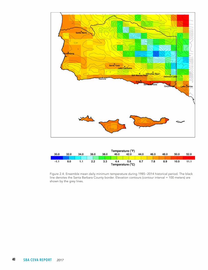
40 SBA CEVA REPORT 2017
Figure 2.4. Ensemble mean daily minimum temperature during 1985−2014 historical period. The black line denotes the Santa Barbara County border. Elevation contours (contour interval = 100 meters) are shown by the grey lines.
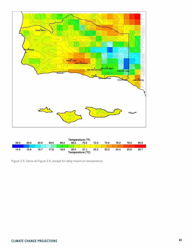
41CLIMATE CHANGE PROJECTIONS
Figure 2.5. Same as Figure 2.4, except for daily maximum temperature.
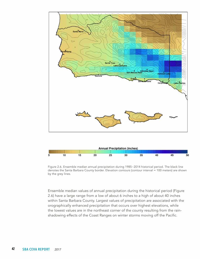
42 SBA CEVA REPORT 2017
Ensemble median values of annual precipitation during the historical period (Figure 2.6) have a large range from a low of about 6 inches to a high of about 40 inches within Santa Barbara County. Largest values of precipitation are associated with the orographically enhanced precipitation that occurs over highest elevations, while the lowest values are in the northeast corner of the county resulting from the rain-shadowing effects of the Coast Ranges on winter storms moving off the Pacific.
Figure 2.6. Ensemble median annual precipitation during 1985−2014 historical period. The black line denotes the Santa Barbara County border. Elevation contours (contour interval = 100 meters) are shown by the grey lines.

43CLIMATE CHANGE PROJECTIONS
Figure 2.7 shows the ensemble median values of the number of wet days over Santa Barbara County during the historical period. The largest values of up to about 30 days per year are in the highest elevations of Santa Barbara County. Relatively high values are also found along the south-facing coastal slopes in the western part of the county. Significantly lower values of about 8-10 days per year are noted in extreme northeastern Santa Barbara County and are again associated with rain-shadowing effects.
Figure 2.7. Ensemble median number of wet days per year during 1985−2014 historical period. A wet day is defined as day with precipitation >0.25”.
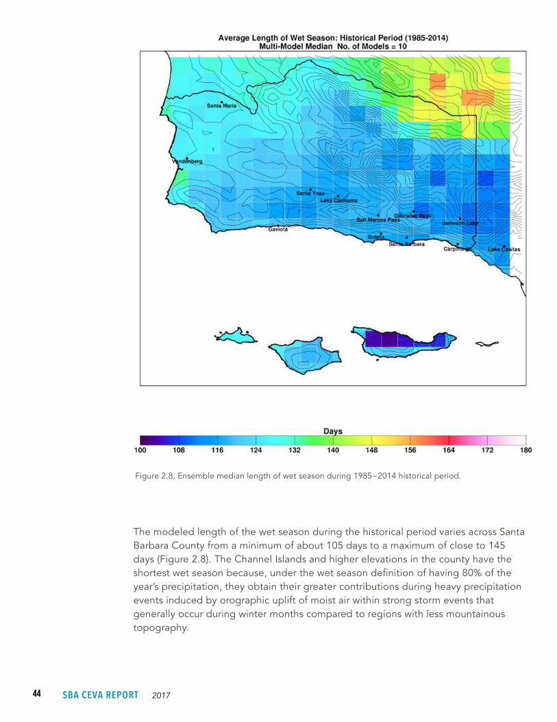
44 SBA CEVA REPORT 2017
The modeled length of the wet season during the historical period varies across Santa Barbara County from a minimum of about 105 days to a maximum of close to 145 days (Figure 2.8). The Channel Islands and higher elevations in the county have the shortest wet season because, under the wet season definition of having 80% of the year’s precipitation, they obtain their greater contributions during heavy precipitation events induced by orographic uplift of moist air within strong storm events that generally occur during winter months compared to regions with less mountainous topography.
Figure 2.8. Ensemble median length of wet season during 1985−2014 historical period.

45CLIMATE CHANGE PROJECTIONS
C L I M A T E M O D E L I N G : P R O J E C T I O N S
Increasing trends in both daily minimum and maximum temperature are projected by all models and both emission scenarios. Projected differences in daily minimum and maximum temperature (relative to their historical means) are displayed in Figures 2.9 and 2.10, respectively. The projected temperature increases are largest with the RCP 8.5 emission scenario compared to the RCP 4.5 scenario and the difference between these two scenarios becomes much more apparent in the latter part of the century. Projected average temperature increases with RCP 8.5 scenario are about 1.5°F by year 2030, 3.0°F by year 2050 and up to 6-7°F at the end of the century.
The magnitude of the projected differences in daily maximum temperature are slightly larger and on the order of 0.1-0.2°F compared to those for daily minimum temperature. These downscaled projected temperature differences show modest spatial variation on the order of 1-2°F with generally larger values over inland and mountainous regions and smaller values over coastal regions and offshore islands. The small temperature increases projected for the islands and coastal regions is due at least in part to the thermal buffering effect of the Pacific Ocean which will be slower to warm than land areas due to larger heat capacity of water compared to land.
Figure 2.9. Ensemble mean difference of daily minimum temperature between 2020−2039 period (left column), 2040−2059 period (middle column), 2080−2099 period (right column) and 1985−2014 historical period for emission scenarios RCP 4.5 (top row) and RCP 8.5 (bottom row).
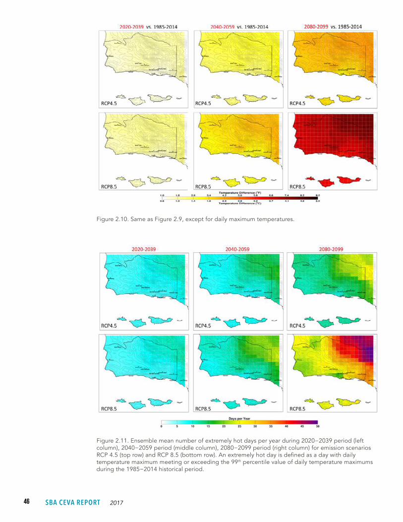
46 SBA CEVA REPORT 2017
Figure 2.10. Same as Figure 2.9, except for daily maximum temperatures.
Figure 2.11. Ensemble mean number of extremely hot days per year during 2020−2039 period (left column), 2040−2059 period (middle column), 2080−2099 period (right column) for emission scenarios RCP 4.5 (top row) and RCP 8.5 (bottom row). An extremely hot day is defined as a day with daily temperature maximum meeting or exceeding the 99th percentile value of daily temperature maximums during the 1985−2014 historical period.

47CLIMATE CHANGE PROJECTIONS
Figure 2.11 shows the projected annual number of extremely hot days. Similar to a broader pattern of increasing heat waves across the Southwestern United States (Gershunov et al. 2013), the number of extremely hot days is projected to increase across the county relative to the 3-4 days during the historical period with the magnitude increasing in time. These hottest days will occur when climate warming is amplified by weather patterns similar to those that drive hot spells during recent historic decades; e.g., under an atmospheric flow regime which results in subsiding air masses, driving the coastal marine layer offshore (Gershunov and Guirguis 2012) and depleting the coastal stratus that often cools the region (Iacobellis and Cayan 2013). The largest increases are found in higher elevations and extreme northeastern portions of Santa Barbara County where projected number of extreme hot days reach about 9-14 days by 2030, 18-24 days by 2050, and 36-45 days by 2090 under RCP 8.5 emission scenario. Smaller, but still significant increases in extreme hot days are projected for the coastal regions. For the Goleta−Santa Barbara−Carpinteria coastal strip, the projected number of hot days with RCP 8.5 emission scenario are 6-8 by 2030, 8-13 by 2050, and 19-33 by 2090.
Figure 2.12. Difference in ensemble median annual precipitation between 2020−2039 period (left column), 2040−2059 period (middle column), 2080−2099 period (right column) and 1985−2014 historical period for emission scenarios RCP 4.5 (top row) and RCP 8.5 (bottom row).
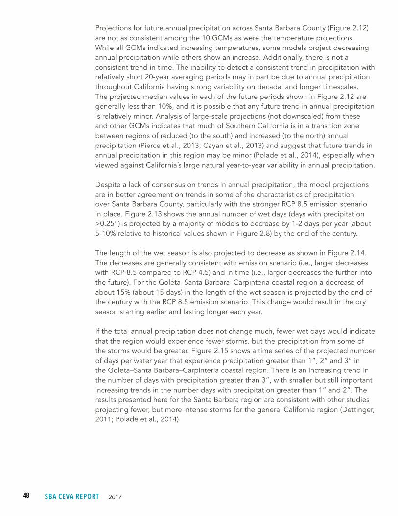
48 SBA CEVA REPORT 2017
Projections for future annual precipitation across Santa Barbara County (Figure 2.12) are not as consistent among the 10 GCMs as were the temperature projections. While all GCMs indicated increasing temperatures, some models project decreasing annual precipitation while others show an increase. Additionally, there is not a consistent trend in time. The inability to detect a consistent trend in precipitation with relatively short 20-year averaging periods may in part be due to annual precipitation throughout California having strong variability on decadal and longer timescales. The projected median values in each of the future periods shown in Figure 2.12 are generally less than 10%, and it is possible that any future trend in annual precipitation is relatively minor. Analysis of large-scale projections (not downscaled) from these and other GCMs indicates that much of Southern California is in a transition zone between regions of reduced (to the south) and increased (to the north) annual precipitation (Pierce et al., 2013; Cayan et al., 2013) and suggest that future trends in annual precipitation in this region may be minor (Polade et al., 2014), especially when viewed against California’s large natural year-to-year variability in annual precipitation.
Despite a lack of consensus on trends in annual precipitation, the model projections are in better agreement on trends in some of the characteristics of precipitation over Santa Barbara County, particularly with the stronger RCP 8.5 emission scenario in place. Figure 2.13 shows the annual number of wet days (days with precipitation >0.25”) is projected by a majority of models to decrease by 1-2 days per year (about 5-10% relative to historical values shown in Figure 2.8) by the end of the century.
The length of the wet season is also projected to decrease as shown in Figure 2.14. The decreases are generally consistent with emission scenario (i.e., larger decreases with RCP 8.5 compared to RCP 4.5) and in time (i.e., larger decreases the further into the future). For the Goleta–Santa Barbara–Carpinteria coastal region a decrease of about 15% (about 15 days) in the length of the wet season is projected by the end of the century with the RCP 8.5 emission scenario. This change would result in the dry season starting earlier and lasting longer each year.
If the total annual precipitation does not change much, fewer wet days would indicate that the region would experience fewer storms, but the precipitation from some of the storms would be greater. Figure 2.15 shows a time series of the projected number of days per water year that experience precipitation greater than 1”, 2” and 3” in the Goleta–Santa Barbara–Carpinteria coastal region. There is an increasing trend in the number of days with precipitation greater than 3”, with smaller but still important increasing trends in the number days with precipitation greater than 1” and 2”. The results presented here for the Santa Barbara region are consistent with other studies projecting fewer, but more intense storms for the general California region (Dettinger, 2011; Polade et al., 2014).

49CLIMATE CHANGE PROJECTIONS
Figure 2.13. Same as Figure 2.12, except for ensemble median annual number of wet days.
Figure 2.14. Same as Figure 2.12, except for ensemble median length of wet season.
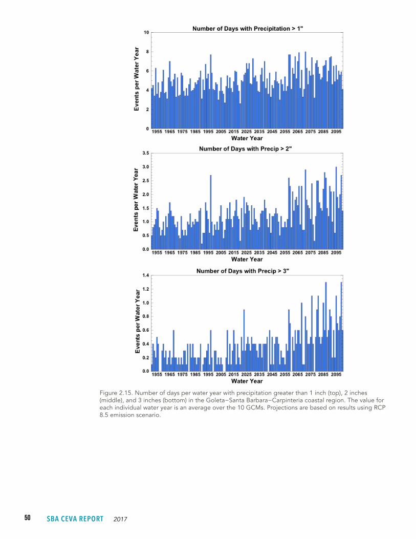
50 SBA CEVA REPORT 2017
Figure 2.15. Number of days per water year with precipitation greater than 1 inch (top), 2 inches (middle), and 3 inches (bottom) in the Goleta−Santa Barbara−Carpinteria coastal region. The value for each individual water year is an average over the 10 GCMs. Projections are based on results using RCP 8.5 emission scenario.

51CLIMATE CHANGE PROJECTIONS
California, and Southern California in particular, has the highest observed natural variability of year-to-year precipitation in the conterminous United States (Dettinger et al., 2011; Iacobellis et al., 2016). Within this strong natural interannual variability are multi-year periods of consecutive wet and dry years that often lead to significant flood and drought conditions impacting a wide range of ecosystems.
The coefficient of variation of a distribution is defined as the standard deviation divided by the mean and has previously been used to measure interannual precipitation variability (Dettinger et al., 2011). To measure projected changes in year-to-year variability of precipitation, the coefficient of variation was calculated for water year precipitation over the 1951–2000 and 2051–2100 periods for each GCM. Eight of the 10 GCMs project increasing values in the coefficient of variation for water year precipitation during the 2051–2100 period relative to the 1951–2000 period. The changes ranged from -11% to +50% with a median value of +11%. A projected increase in the interannual variability of precipitation would enhance the region’s already strong natural variability resulting in more frequent and intense multi-year wet and dry periods leading to increasing stress on susceptible ecosystems
C L I M A T E M O D E L I N G : S E A S O N A L P R O J E C T I O N S
The results presented above are annual values, that is all 12 months of the year were included in the period means (or medians). Below, 3-month seasonal means (or medians) are presented for the selected sub-region of Santa Barbara County that includes the cities of Goleta, Santa Barbara and Carpinteria (Figure 2.12). The seasonal values are calculated over months December-February (DJF), March-May (MAM), June-August (JJA), and September-November (SON). The means (medians) calculated using emission scenarios RCP 4.5 and RCP 8.5 are shown in Tables 2.3 and 2.4, respectively.
The largest projected temperature increases are found during the fall SON season, while the smallest increases are during the summer JJA season and are consistent for daily minimum and maximum temperature, all three future periods and both emission scenarios. The seasonal changes in precipitation show much of the same inconsistencies that were noted for the annual values. However, one exception is a decrease in fall (SON) precipitation for both emission scenarios and all time periods. Projected precipitation during spring months (MAM) shows either no net change or slight decreases. This pattern of reduced precipitation during the fall and spring seasons is also evident in the projected seasonal changes in the number of dry days. These seasonal results are in qualitative agreement with the earlier finding of a projected reduction in the length of the wet season, which is less precipitation in the transition seasons and more during the winter season.
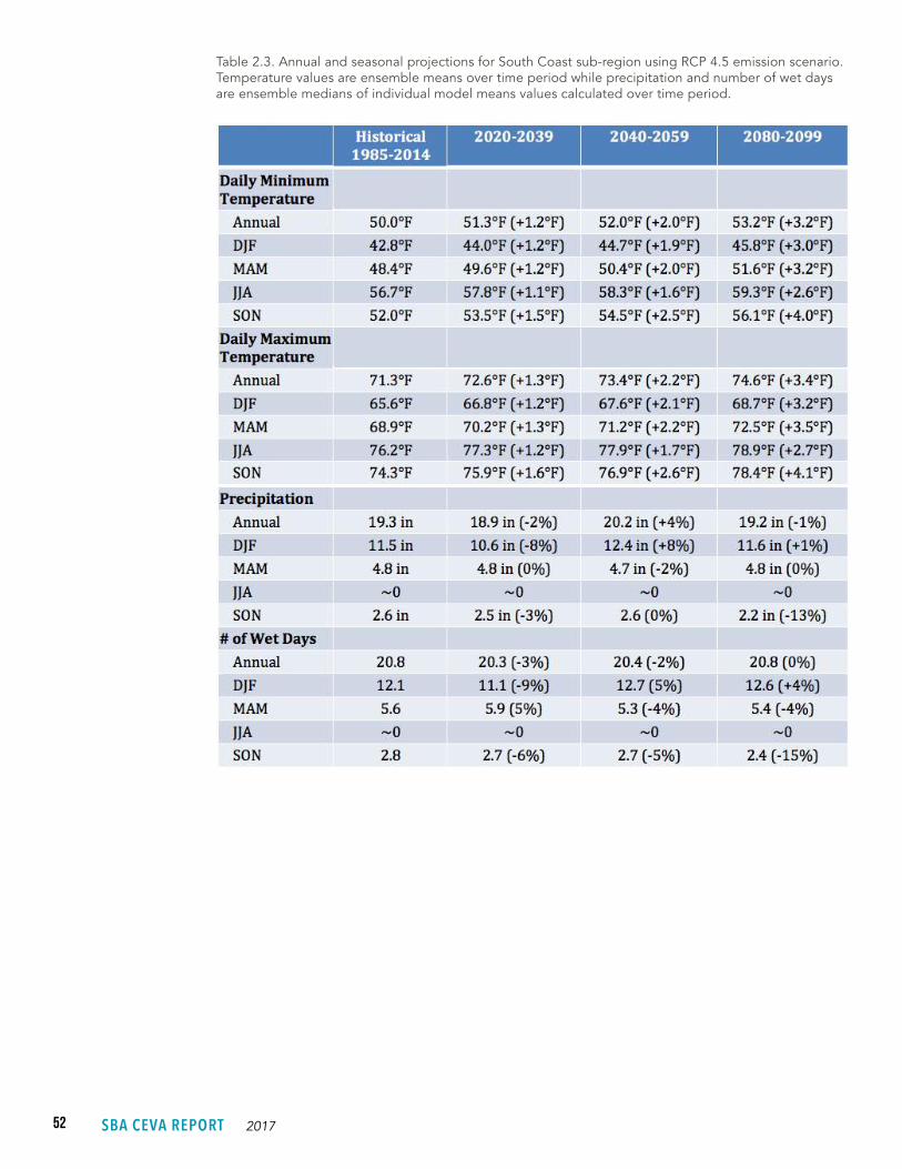
52 SBA CEVA REPORT 2017
Table 2.3. Annual and seasonal projections for South Coast sub-region using RCP 4.5 emission scenario. Temperature values are ensemble means over time period while precipitation and number of wet days are ensemble medians of individual model means values calculated over time period.
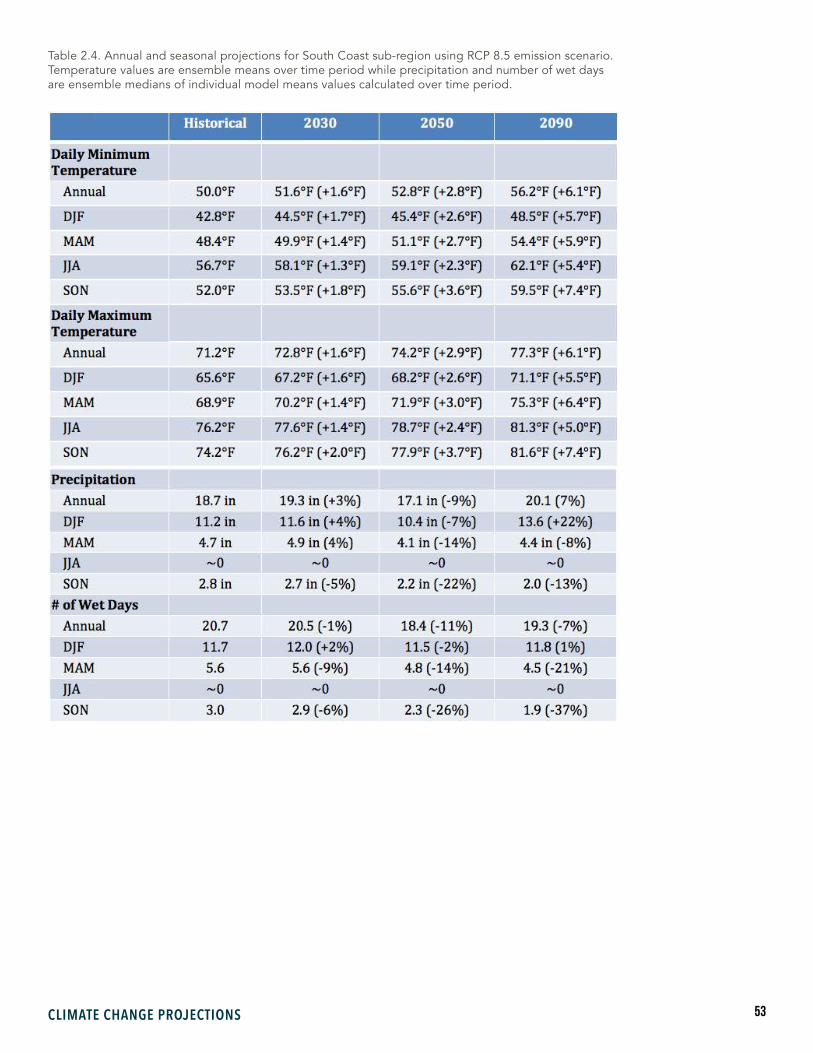
53CLIMATE CHANGE PROJECTIONS
Table 2.4. Annual and seasonal projections for South Coast sub-region using RCP 8.5 emission scenario. Temperature values are ensemble means over time period while precipitation and number of wet days are ensemble medians of individual model means values calculated over time period.
54 SBA CEVA REPORT 2017
2.3.2 WATER LEVEL MODELING RESULTS/DISCUSSION
Hourly values of the meteorological component of the residual water level were produced using the regression model and output from each of the eight GCMs run with either RCP 4.5 or RCP 8.5 emission scenario. These hourly values of the meteorological component of the residual water level were then combined with predictions of astronomical tides and one of the three SLR scenarios to produce an hourly time series of Total Water Level at Santa Barbara extending from 1950 to 2100. Figure 2.16 shows annual Mean Sea Level anomalies using output from the GCMs run with emission scenario RCP 8.5. Each of the thin lines in this figure represent a time series that used a particular GCM to produce values of the meteorological component of the residual water level. Values during the historical period used observed values of SLR and are shown by thin grey lines.
The variability between lines of the same color represent differences in the meteorological component of the residual water level term produced by the individual GCMs. While there is some variation between individual GCMs, it is clear the dominant factor determining overall sea level in the future is the choice of the SLR scenario. Using the mid-range SLR scenario and RCP 8.5 emission scenario sea level heights are projected to increase about 15 cm by 2030, 30 cm by 2050 and 90 cm by the end of the century. Results using output from the GCMs run with the RCP 4.5 emission scenario to produce the meteorological component of the residual water level term are similar.

55CLIMATE CHANGE PROJECTIONS
Figure 2.16. Annual sea level anomalies at Santa Barbara. Model produced values during the 1950–2005 historical period are shown as grey lines, while modeled projections during the 2005–2100 period are shown by the green, blue and red lines with the color denoting a particular NRC SLR scenario. The black curve fragments between 1990 and 2014 are based on a limited set of observations at Santa Barbara Harbor.
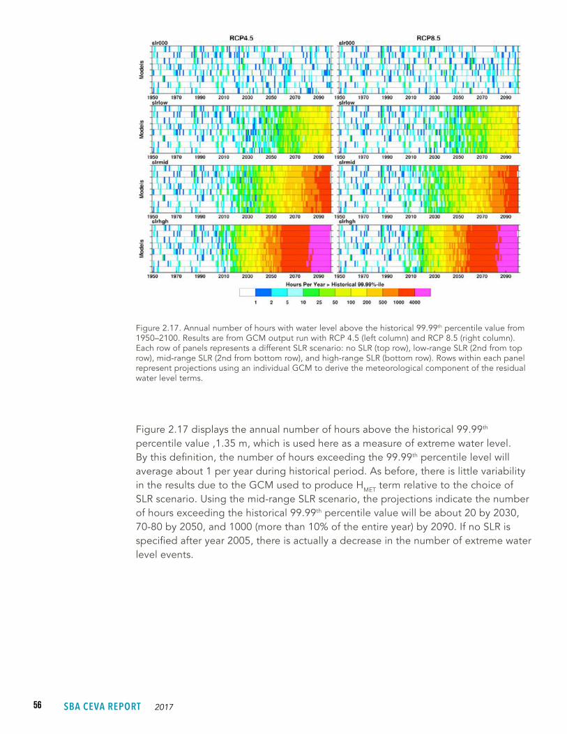
56 SBA CEVA REPORT 2017
Figure 2.17. Annual number of hours with water level above the historical 99.99th percentile value from 1950–2100. Results are from GCM output run with RCP 4.5 (left column) and RCP 8.5 (right column). Each row of panels represents a different SLR scenario: no SLR (top row), low-range SLR (2nd from top row), mid-range SLR (2nd from bottom row), and high-range SLR (bottom row). Rows within each panel represent projections using an individual GCM to derive the meteorological component of the residual water level terms.
Figure 2.17 displays the annual number of hours above the historical 99.99th percentile value ,1.35 m, which is used here as a measure of extreme water level. By this definition, the number of hours exceeding the 99.99th percentile level will average about 1 per year during historical period. As before, there is little variability in the results due to the GCM used to produce HMET term relative to the choice of SLR scenario. Using the mid-range SLR scenario, the projections indicate the number of hours exceeding the historical 99.99th percentile value will be about 20 by 2030, 70-80 by 2050, and 1000 (more than 10% of the entire year) by 2090. If no SLR is specified after year 2005, there is actually a decrease in the number of extreme water level events.
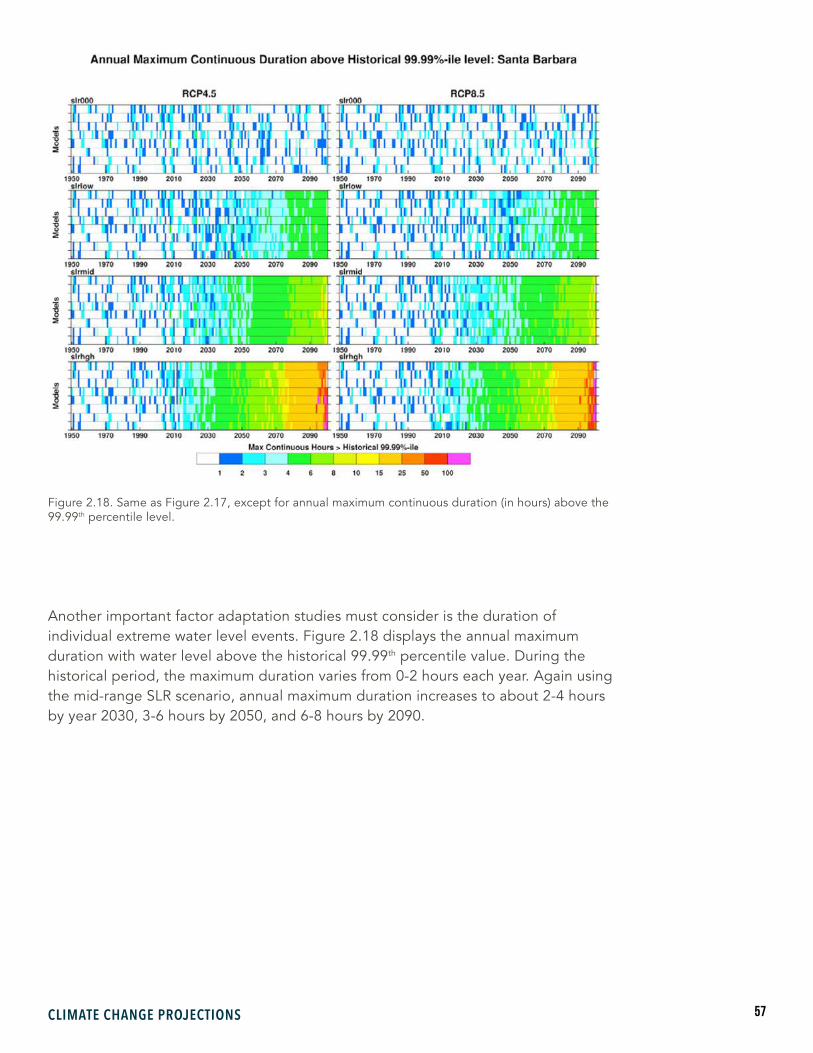
57CLIMATE CHANGE PROJECTIONS
Another important factor adaptation studies must consider is the duration of individual extreme water level events. Figure 2.18 displays the annual maximum duration with water level above the historical 99.99th percentile value. During the historical period, the maximum duration varies from 0-2 hours each year. Again using the mid-range SLR scenario, annual maximum duration increases to about 2-4 hours by year 2030, 3-6 hours by 2050, and 6-8 hours by 2090.
Figure 2.18. Same as Figure 2.17, except for annual maximum continuous duration (in hours) above the 99.99th percentile level.

58 SBA CEVA REPORT 2017
Figure 2.19. Number of hours with water level exceeding the historical 99.99th percentile level at Santa Barbara for individual months. Values shown are averaged over historical period (top panel), 2035–2064 (middle panel), and 2070–2099 (bottom panel). Projections based on low-range (green), mid-range (blue) and high-range (red) SLR scenarios. Model results during historical period are shown in grey while observations are shown in black. Notes: i) the scale on the vertical axis of each panel varies; ii) the relatively short 12-year period of observations at Santa Barbara makes comparison to modeled events difficult.
The number of hours with extreme water level at Santa Barbara for individual months is shown in Figure 2.19. During the historical period, extreme water level events are primarily limited to months June-August and November-February. This is due to the highest astronomical tides that occur in these months as well as strong winter storms that impact water level that occur during the winter months.

59CLIMATE CHANGE PROJECTIONS
By mid-century, the number of extreme water level events increases and occur in more months. With the high-range SLR scenario, extreme water level events occur in all months. By the end of the century, the number of hours with extreme water levels increases dramatically in all months.
2.4 KEY FINDINGS
• All climate models examined are consistent in projecting increasing temperatures across Santa Barbara County throughout the 21st century. The average magnitude of the projected temperature increases using the RCP 8.5 emission scenario are about 1.5°F by 2030, 3°F by 2050, and 6-7°F by 2090. The temperature increases are more pronounced in the inland and mountain areas of the county and less along the coast and offshore islands.
• The number of extremely hot days (as measured by current historical values) is projected to increase significantly. Using the historical 99th percentile as a reference, the models project more than a doubling by 2050 and a nearly 10-fold increase by 2090. These projected changes are useful for assessing impacts to ecosystems.
• The median of the 10-model ensemble of projections indicates that annual precipitation amounts for Santa Barbara County are not projected to change significantly during the 21st century. However, the individual models produced inconsistent projections of annual precipitation with some showing reduced and others increased amounts relative to current historical values. Consequently, there is considerable uncertainty in this result.
• The model projections are consistent regarding frequency and variability of future precipitation indicating occasionally more intense storms, a reduction in the number of wet (rainy) days, and a decrease in the length of the wet season. These changes, e.g., longer spells of dry days and a longer dry season, would likely have important consequences to terrestrial and coastal ecosystems (e.g., increase the risk of wildfire) but those are generally not explored in this report.
• A majority of the models project an increase in the year-to-year variability of annual precipitation by the second half of the 21st century that would increase the likelihood of extended periods of drought.
• Sea level heights are projected to increase significantly during the 21st century. Even the most optimistic sea level rise scenario examined produced notable increases in both the frequency and duration of high water levels.

60 SBA CEVA REPORT 2017
3. Watershed RunoffAUTHORS: JOHN MELACK, EDWARD BEIGHLEY
3.1 INTRODUCTION
Watershed runoff is important to Santa Barbara area coastal ecosystems influencing creeks, beaches and wetlands. Santa Barbara area watersheds extend from ridge tops in the Los Padres National Forest and Santa Ynez Mountains to the ocean. These south-sloping coastal watersheds are subjected to a Mediterranean climate and receive the majority of annual precipitation in winter (see Climate of the Santa Barbara Area, pg. 31). A total area of 305mi2 (790 km2) (ranging from .4-47mi2 [1-123 km2]), including 135 watersheds, drain into the northern coast of Santa Barbara Channel (Figure 3.1). The topography of these coastal watersheds is characterized as mountainous headwaters and gently sloping coastal plains. Ridge-top elevations increase from approximately 300 to 1400 m from west to east along the coast, and land uses on the coastal plain and foothills change from mostly rangeland to a combination of urban and agricultural lands. At higher elevations throughout and
Callie B
owd
ish

61WATERSHED RUNOFF
on the lower elevations in undeveloped areas, coastal sage scrub and evergreen chaparral communities occur. The mountainous portions of the catchments have thin, well drained, fine silt loams overlying fractured bedrock, while on the coastal plains, the soils are deep alluvial deposits (National Resources Conservation Service, 1995; Minor et al., 2003).
The Mission Creek watershed includes much of the City of Santa Barbara in its lower reaches. The watershed, nearly 50% urban, contains steep undeveloped canyons, coastal mesas and coastal plains (Goodridge and Melack 2012). Atascadero, Maria Ygnacio, San Jose, San Pedro, Tecolotito and Carneros creeks drain approximately 47 square miles of watersheds into Goleta Slough. Santa Monica and Franklin creeks drain into Carpinteria Salt Marsh. Devereux Creek flows into Devereux Slough, with its watershed extending only into the lower foothills and draining largely suburban areas.
Few studies have investigated impacts of future climate conditions on stream discharges (the volume of water per unit time, e.g. m3 s-1 or ft3 s-1), although significant changes in precipitation and temperature are expected. For example, Warner et al. (2015) suggest that mean winter precipitation along the West Coast of the U.S. may increase by 11% to18% by the end of this century, and the frequency of precipitation extremes may increase by up to 290% under the highest emission pathway (i.e., RCP 8.5). Dettinger (2011) also found that the frequency and intensity of atmospheric rivers will increase under high emission scenarios, which will increase the potential for both more frequent and more severe floods in California. Understanding how future climate conditions translate to variations in stream discharge is the focus of this watershed analysis. In this section, downscaled climate model outputs were used in a high-resolution hydrologic model providing daily stream discharge for coastal Santa Barbara County watersheds (Figure 3.1). Results are intended to provide planners, policy makers and water resource managers with quantitative insights on how future stream discharges compare to current conditions. The watershed analysis builds on established methods and past hydrologic studies focused on coastal Santa Barbara County supported by the Santa Barbara Coastal Long-Term Ecological Research project (Beighley et al., 2005, 2008; Beighley et al., 2003).
3.2 METHODS
For the watershed analysis, the study region is defined by the watersheds draining into the Santa Barbara Channel from just west of the Ventura River to just east of Point Conception (Figure 3.1). The combined land area is roughly 780 km2 with 135 watersheds ranging from 1 to 123 km2. The study region contains eight U.S. Geological Survey stream gauging stations with relatively long historical records (Table 3.1). While this study includes all watersheds in the region, this report focuses on the six drainage systems shown in Figure 3.1 (Table 3.2).
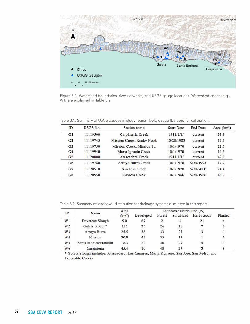
62 SBA CEVA REPORT 2017
Figure 3.1. Watershed boundaries, river networks, and USGS gauge locations. Watershed codes (e.g., W1) are explained in Table 3.2
Table 3.1. Summary of USGS gauges in study region, bold gauge IDs used for calibration.
Table 3.2. Summary of landcover distribution for drainage systems discussed in this report.
63WATERSHED RUNOFF
A hydrologic model uses downscaled precipitation and temperatures from 10 climate models and two climate scenarios (RCP 4.5 and 8.5) (see Climate section) to simulate stream discharge for the period 1950–2100 and assess the potential impacts of future climate conditions on stream discharges. Specifically, daily precipitation and temperature downscaled to a spatial resolution of 6 km using Localized Constructed Analogs (Pierce et al., 2014) are used to drive the Hillslope River Routing (HRR) model (Beighley et al., 2009) to estimate past (1950–2005) and future (2006–2100) stream discharges. The HRR model builds on previous modeling efforts in coastal Santa Barbara County (Beighley et al., 2005, 2008; Beighley et al., 2003). The model combines long-term simulation capabilities with specific event-focused rainfall-runoff processes and hydraulic routing at fine spatial and temporal scales ideally suitable for flood modeling (Ray et al., 2016; Seyyedi et al., 2015; Yoon et al., 2016). Daily gauge-based precipitation and temperature data with a spatial resolution of 6 km (3.73 mile) (Livneh et al., 2015) are used to calibrate and validate the HRR model to U.S. Geological Survey stream discharge measurements at 5 sites (Figure 3.1; Table 3.1). Streamflow statistics derived from each climate model for the historical period (1950–2005) are compared to observed statistics and used to assess how well each climate model represents past conditions. This assessment provides insights on the similarity of 10 models providing the ensemble of simulated future stream discharges. Future stream discharges for the first (2006–2061) and second (2045–2100) half of the projections are presented in terms of changes relative to recent conditions (1950–2005).
In the HRR model, the watersheds are delineated into smaller catchments (i.e., model units) and the associated river reaches connecting the catchments. Model units are roughly 1 km2. Within each model unit HRR simulates: (a) vertical water and energy balance through vegetation and soil layers; (b) lateral hydraulic transport from upland areas; and (c) channel hydraulics. The kinematic approximation is used for simulating surface and groundwater runoff from hillslopes to channels; and diffusion wave routing is used for channel discharge. Potential evapotranspiration (ET) is estimated using the Priestley and Taylor method (Priestley and Taylor, 1972) and the Food and Agriculture Organization of the United Nations (FAO) limited climate data approximations (Allen et al., 1998), which are largely based on temperature (daily minimum, maximum and mean). This approach enables estimates of future evapotransition based on the downscaled GCM temperature forecasts.
Given the importance of runoff events in the region, we highlight the HRR components related to simulation of events. To generate surface runoff, a runoff coefficient (C) approach is used (i.e., runoff at time, t, is C x Pt ), where Pt is rainfall at time t and the C varies based on land cover. Here, two runoff coefficients (initial and wet) are used for each model unit, with a soil moisture threshold to switch between to the two coefficients. For the gauged watersheds, the three parameters are determined based on calibration. For the ungauged watershed, a regression equation is developed to related calibrated runoff coefficients to gauged watershed land cover characteristics. The regression equation is then used to assigned runoff coefficients to all model units based on their land cover characteristics (e.g., C =

64 SBA CEVA REPORT 2017
mU + b, where U is percent urban within a model unit, and m and b are regression coefficients relating the fraction of urban land cover and the effective runoff coefficient). Based on the availability of stream discharge data, the calibration period is 1984–2013. The model inputs are gauge-based, gridded precipitation and temperatures (Livneh et al., 2015). USGS stream discharge measurements from 5 gauges are used for calibration (Figure 3.1, Table 3.1). For the days with missing data within the calibration period, relationships between discharges at the gauge with missing data and those at its neighboring gauge were developed and used to estimate the missing values. The parameters included in the calibration that impact lateral and vertical transport and surface runoff generation processes include: ks (coefficient to adjust surface roughness), kv (coefficient to adjust vertical hydraulic conductivity), kh (coefficient to adjust horizontal hydraulic conductivity), θt (threshold in soil moisture separating dry and wet runoff conditions), C1 (runoff coefficient for θ < θt ), and C2 (runoff coefficient for θ ≥ θt ). The parameter ranges are predefined based on the hydrological characteristics of the region and previous modeling experience in the region (Beighley et al., 2005, 2008; Beighley et al., 2003).
The performance metrics used for calibration are bias (to assess water balance), annual peak error (to assess high flow conditions), and the mean squared error of daily log-transformed flows (to assess recession flows and baseflow conditions). The three metrics are combined into a single multivariate performance metric:
where are mean bias, mean peak error and mean squared error, respectively, based on averaging annual values over the entire calibration period.
An automated calibration procedure was used to estimate these parameters. The procedure consisted of randomly selecting parameter values from pre-defined parameter ranges, simulating with the HRR model, determining the multivariate performance metric (Eq. 3.1) at each gauge, and averaging the performance metric values from each gauge. This process was repeated thousands of times. The parameter set resulting in the minimum multivariate performance metric averaged over all gauges was selected as the optimal set.
The calibration was performed using gauge-based precipitation and temperature. Next, the calibrated HRR model was simulated using the global climate model (GCM) inputs for the historical period (1950–2005) and future conditions (2006–2061) and (2045–2100). To assess the applicability of the GCM forcings in the region of study, the year-to-year viability of hydrological response (i.e., stream discharge) for both observations and HRR simulations using the historical period GCM forcings was determined. Rather than assessing temperature and precipitation directly, we quantify
(3.1)
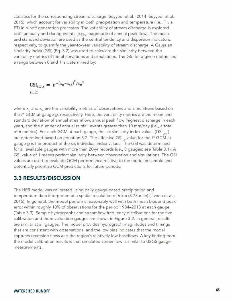
65WATERSHED RUNOFF
statistics for the corresponding stream discharge (Seyyedi et al., 2014; Seyyedi et al., 2015), which account for variability in both precipitation and temperature (i.e., T via ET) in runoff generation processes. The variability of stream discharge is explored both annually and during events (e.g., magnitude of annual peak flow). The mean and standard deviation are used as the central tendency and dispersion indicators, respectively, to quantify the year-to-year variability of stream discharge. A Gaussian similarity index (GSI) (Eq. 3.2) was used to calculate the similarity between the variability metrics of the observations and simulations. The GSI for a given metric has a range between 0 and 1 is determined by:
where xg and xs,i are the variability metrics of observations and simulations based on the ith GCM at gauge g, respectively. Here, the variability metrics are the mean and standard deviation of annual streamflow, annual peak flow (highest discharge in each year), and the number of annual rainfall events greater than 10 mm/day (i.e., a total of 6 metrics). For each GCM at each gauge, the six similarity index values (GSIi,g,x ) are determined based on equation 3.2. The effective GSIi,g value for the ith GCM at gauge g is the product of the six individual index values. The GSI was determined for all available gauges with more than 20-yr records (i.e., 8 gauges; see Table 3.1). A GSI value of 1 means perfect similarity between observation and simulations. The GSI values are used to evaluate GCM performance relative to the model ensemble and potentially prioritize GCM predictions for future periods.
3.3 RESULTS/DISCUSSION
The HRR model was calibrated using daily gauge-based precipitation and temperature data interpreted at a spatial resolution of 6 km (3.73 mile) (Livneh et al., 2015). In general, the model performs reasonably well with both mean bias and peak error within roughly 10% of observations for the period 1984–2013 at each gauge (Table 3.3). Sample hydrographs and streamflow frequency distributions for the five calibration and three validation gauges are shown in Figure 3.2. In general, results are similar at all gauges. The model provides hydrograph magnitudes and timings that are consistent with observations, and the low bias indicates that the model captures recession flows and the region’s relatively low baseflows. A key finding from the model calibration results is that simulated streamflow is similar to USGS gauge measurements.
(3.2)
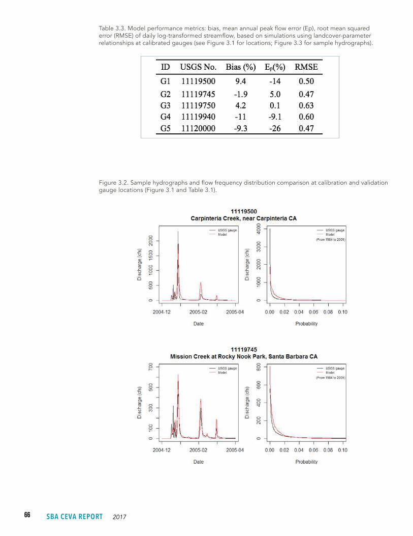
66 SBA CEVA REPORT 2017
Table 3.3. Model performance metrics: bias, mean annual peak flow error (Ep), root mean squared error (RMSE) of daily log-transformed streamflow, based on simulations using landcover-parameter relationships at calibrated gauges (see Figure 3.1 for locations; Figure 3.3 for sample hydrographs).
Figure 3.2. Sample hydrographs and flow frequency distribution comparison at calibration and validation gauge locations (Figure 3.1 and Table 3.1).
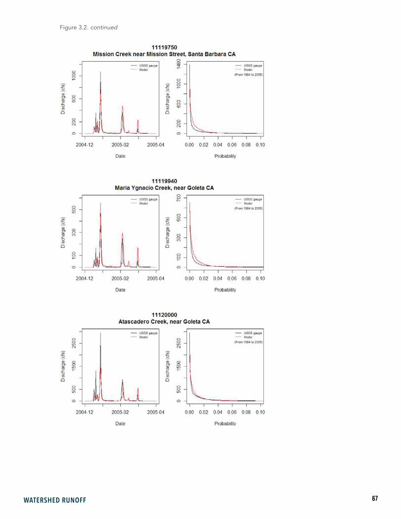
67WATERSHED RUNOFF
Figure 3.2. continued
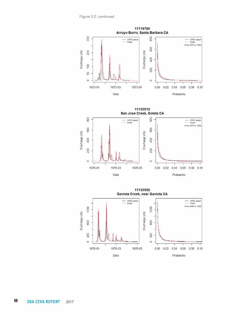
68 SBA CEVA REPORT 2017
Figure 3.2. continued

69WATERSHED RUNOFF
Next, daily streamflows were simulated using the calibrated HRR model and the daily downscaled precipitation and temperature derived from the 10 GCMs for the two emission scenarios. Three periods were considered: historical 1950–2005 and future (2006–2061 and 2045–2100). For the historical period, 10 simulated daily stream discharge series were generated for all watersheds shown in Figure 3.1 (i.e., 1 per GCM; no RCP scenario for historical period). For the future period, 20 simulated daily stream discharge series were generated for each watershed (i.e., 2 for each GCM; one for RCP 4.5 and one for 8.5).
One common challenge when considering the potential impacts of climate change is the variability of results between models. Here, the Gaussian similarity index (GSI) is used. The GSI for streamflow observations at the 8 gauges and simulation streamflow derived from GCM projections are shown in Figure 3.3. Based on the median GSI value (i.e., median of the 8 GSI values; one for each gauge location for a given model), the models appear to perform similarly, with the possible exception of the MIROC5 model. The MIROC5 model has the lowest median GSI, and its minimum and maximum GSI values are the lowest minimum and maximum values for all models. However, the variations between models are still relatively small, and no models appear to be clearly different from the others. Although these results are for the historical period, it is reasonable to suggest models with higher GSI will be more representative of future conditions (Dai, 2016). Based on the relatively consistent GSI values, the results for future conditions (discussed next) include all 10 models with specific focus on median changes from the model ensemble.
Figure 3.3. Gaussian similarity index (GSI) for simulated stream discharges for 1950–2005; whisker indicate range of values (dashed lines), box is 1st to 3rd quartiles and line is median of GSI at the 8 gauges.
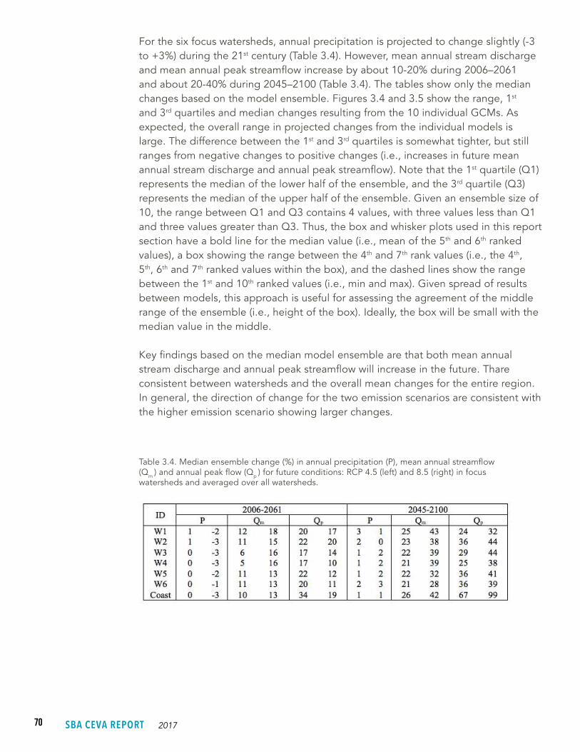
70 SBA CEVA REPORT 2017
For the six focus watersheds, annual precipitation is projected to change slightly (-3 to +3%) during the 21st century (Table 3.4). However, mean annual stream discharge and mean annual peak streamflow increase by about 10-20% during 2006–2061 and about 20-40% during 2045–2100 (Table 3.4). The tables show only the median changes based on the model ensemble. Figures 3.4 and 3.5 show the range, 1st and 3rd quartiles and median changes resulting from the 10 individual GCMs. As expected, the overall range in projected changes from the individual models is large. The difference between the 1st and 3rd quartiles is somewhat tighter, but still ranges from negative changes to positive changes (i.e., increases in future mean annual stream discharge and annual peak streamflow). Note that the 1st quartile (Q1) represents the median of the lower half of the ensemble, and the 3rd quartile (Q3) represents the median of the upper half of the ensemble. Given an ensemble size of 10, the range between Q1 and Q3 contains 4 values, with three values less than Q1 and three values greater than Q3. Thus, the box and whisker plots used in this report section have a bold line for the median value (i.e., mean of the 5th and 6th ranked values), a box showing the range between the 4th and 7th rank values (i.e., the 4th, 5th, 6th and 7th ranked values within the box), and the dashed lines show the range between the 1st and 10th ranked values (i.e., min and max). Given spread of results between models, this approach is useful for assessing the agreement of the middle range of the ensemble (i.e., height of the box). Ideally, the box will be small with the median value in the middle.
Key findings based on the median model ensemble are that both mean annual stream discharge and annual peak streamflow will increase in the future. Thare consistent between watersheds and the overall mean changes for the entire region. In general, the direction of change for the two emission scenarios are consistent with the higher emission scenario showing larger changes.
Table 3.4. Median ensemble change (%) in annual precipitation (P), mean annual streamflow (Qm ) and annual peak flow (Qp ) for future conditions: RCP 4.5 (left) and 8.5 (right) in focus watersheds and averaged over all watersheds.

71WATERSHED RUNOFF
One reason for the disproportional increase in stream discharge as compared to precipitation is that the timing of rainfall varies throughout the wet season. In general, as discussed in Section 2 (see Key Findings, Section 2), wet seasons start later and end sooner leading to a shorter overall rainy season. Specifically, the wet season is projected to be 7-8% shorter during 2006–2061 and roughly 10-15% shorter during 2045–2100 (see Climate section for more details) (Table 3.5). The primary reason for the shorter wet season is a later start. Thus, the annual precipitation is likely to be similar but occurring in a shorter rainy season. Figure 3.6 shows the change in wet season duration for all models. Although the range between models is large, the majority of the models indicate a decrease in rainy season duration. The results are generally consistent between watersheds, with the exception of watersheds 5 and 6 (Santa Monica/Franklin and Carpinteria Creeks), which have a noticeably larger range between the 1st and 3rd quartiles.
Figure 3.4. Change of mean annual stream discharge (Qm) for future conditions (2006–2061; RCP 4.5) in focus watersheds and averaged over all watersheds; whiskers are range (dashed), box is 1st to 3rd quartiles and line is median of 10 GCMs.
Figure 3.5. Change of annual peak streamflow (Qp) for future conditions (2006–2061; RCP 4.5) in focus watersheds and averaged over all watersheds; whiskers are range (dashed), box is 1st to 3rd quartiles and line is median of 10 GCMs.
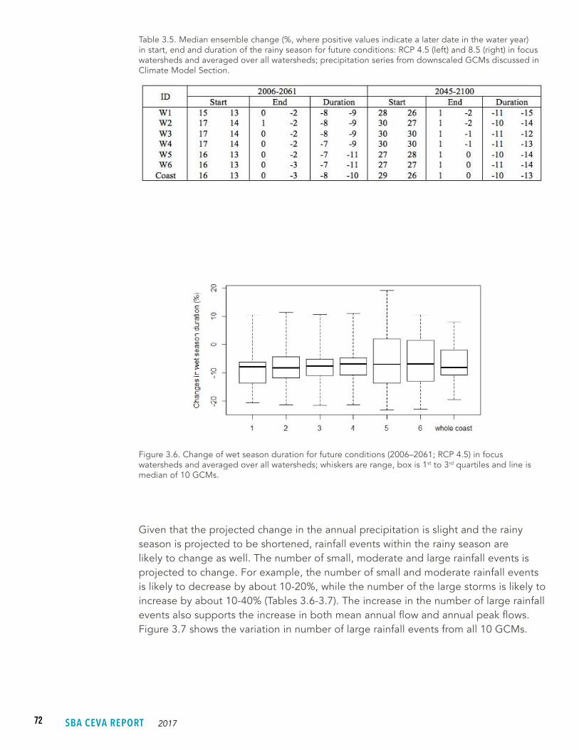
72 SBA CEVA REPORT 2017
Table 3.5. Median ensemble change (%, where positive values indicate a later date in the water year) in start, end and duration of the rainy season for future conditions: RCP 4.5 (left) and 8.5 (right) in focus watersheds and averaged over all watersheds; precipitation series from downscaled GCMs discussed in Climate Model Section.
Figure 3.6. Change of wet season duration for future conditions (2006–2061; RCP 4.5) in focus watersheds and averaged over all watersheds; whiskers are range, box is 1st to 3rd quartiles and line is median of 10 GCMs.
Given that the projected change in the annual precipitation is slight and the rainy season is projected to be shortened, rainfall events within the rainy season are likely to change as well. The number of small, moderate and large rainfall events is projected to change. For example, the number of small and moderate rainfall events is likely to decrease by about 10-20%, while the number of the large storms is likely to increase by about 10-40% (Tables 3.6-3.7). The increase in the number of large rainfall events also supports the increase in both mean annual flow and annual peak flows. Figure 3.7 shows the variation in number of large rainfall events from all 10 GCMs.
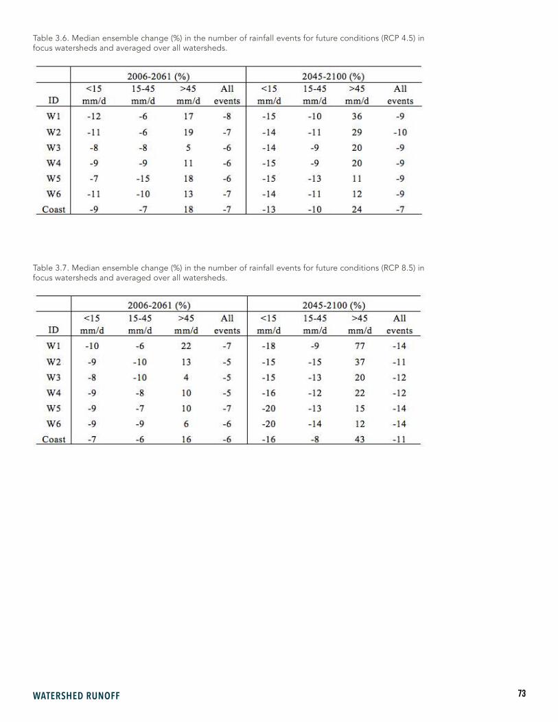
73WATERSHED RUNOFF
Table 3.6. Median ensemble change (%) in the number of rainfall events for future conditions (RCP 4.5) in focus watersheds and averaged over all watersheds.
Table 3.7. Median ensemble change (%) in the number of rainfall events for future conditions (RCP 8.5) in focus watersheds and averaged over all watersheds.

74 SBA CEVA REPORT 2017
Figure 3.7. Change in number of large rainfall events (>45 mm/day) for future conditions (2006–2061; RCP 4.5) in focus watersheds and averaged over all watersheds; whiskers are range, box is 1st to 3rd quartiles and line is median of 10 GCMs.
Table 3.8. Median ensemble change (%) in 100-yr flood magnitude for the future conditions (RCP 4.5 and 8.5) in focus watersheds.
Figure 3.8. Change in 100-yr flood future conditions (2006–2061; RCP 4.5) in focus watersheds; whiskers are range, box is 1st to 3rd quartiles and line is median of 10 GCMs.
75WATERSHED RUNOFF
As a result of changes to annual peak flow magnitudes and year-to-year variability, there is a change in the derived flood frequency distributions. Using the 55-year periods, Flood Frequency Distributions (FFD) were determined for each watershed based on the Log-Person Type III distribution and station skew. Based on these FFDs, the magnitude of the estimated 100-year flood increases by roughly 10-50% for 2006–2061 (except Devereux Slough and Carpinteria Creek) and by about 40-90% (except Devereux Slough) for 2045–2100 (Table 3.8). Figure 3.8 shows the resulting changes in the 100-year flood magnitudes from all 10 GCMs. Compared to changes in annual peak streamflow, the range and median change in the 100-year discharge is much larger. The likely reason for these differences is the change in skewness of the simulated annual peak series for the future conditions. Although 55-years is a reasonable duration to determine flood frequency distributions, extrapolation to larger return periods (e.g., 100-yr) is sensitive to skewness (i.e., measure of the asymmetry of the distribution) of the annual maximum peak discharge series (Ray et al., 2016).
I M P L E M E N T A T I O N A N D I N F O R M A T I O N F O R A D A P T A T I O N
Although annual precipitation remains relatively unchanged, the number of large rainfall events increases. The rainy season is likely to start later, end sooner and to be generally shorter. The shorter season combined with more large rainfall events leads to more runoff (because of wetter initial conditions) and larger peak discharges (resulting from large rainfall events on wetter soils). The larger annual peaks lead to changes in flood frequency distributions (such as increases in 100-yr flood discharges). In general, results for the higher emission scenario (RCP 8.5) indicate similar patterns of changes to that under RCP 4.5, but the magnitude of changes are larger.
Three conclusions regarding projected climate changes in the Santa Barbara area that are likely to have significant influences on stream, wetland and beach ecosystems are a decrease in the length of the wet season that would likely increase the risk of wildfire during the longer dry season, fewer but more intense storms, and increased annual runoff and peak streamflow. Furthermore, projected increases in the year-to-year variability of annual precipitation by the second half of the 21st century would increase the likelihood of extended periods of drought.
Warrick et al. (2015) examined suspended-sediment fluxes in coastal watersheds in the Santa Barbara area and reported a very large range in suspended-sediment concentrations from 1 to over 200,000 mg per liter. Though sediment concentrations were weakly correlated with stream discharge, the majority of sediment flux occurred during only 1% of the time, often associated with peak discharges. With more intense storms projected to occur as the climate changes, the frequency and magnitude of large sediment fluxes are likely to increase. In addition, conversion of native

76 SBA CEVA REPORT 2017
chaparral to non-native grasses may increase soil erosion and landslide frequencies in the region (Gabet and Dunne, 2002; Pinter and Vestal, 2005). As a consequence, sediment deposition in coastal wetlands and inputs to local beaches are likely to increase.
Wildfires are common in the Santa Barbara area, and incineration of vegetation can exacerbate erosion and sediment fluxes, especially during large runoff events (Florsheim et al., 1991; Coombs and Melack, 2012). Sediment yields can increase by an order of magnitude within burned watersheds (Warrick et al., 2015). Projections of shorter wet seasons and longer droughts will further exaggerate fires and their ecosystem impacts.
High temporal and spatial variability in sediment fluxes complicates projections of effects of climate changes among watersheds, as do rare events such as earthquakes or wildfires (García-Ruiz et al., 2013).
3.4 KEY FINDINGS
The key findings from the watershed runoff analysis are:
• Annual runoff and peak streamflow increase by 5-43% and 10-44%, respectively;
• More variability in the magnitude of large flooding events is expected from year to year;
• Design discharges, which are based on fitting annual peak discharges to specific frequency distributions to estimate the probability of exceedance for a given discharge (e.g., 100-yr flood; 1% chance of being exceeded in a given year), are expected to increase even more than projected increases in annual peak discharges; and
• The emissions scenarios (RCP 4.4 and RCP 8.5) result in similar changes, but the higher emission scenario (RCP 8.5) generally results in larger changes suggesting that if emissions are higher, potential hydrologic changes could be even larger.
Dave H
ubb
ard
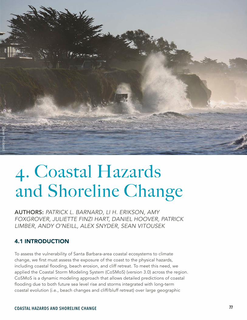
77COASTAL HAZARDS AND SHORELINE CHANGE
4. Coastal Hazards
AUTHORS: PATRICK L. BARNARD, LI H. ERIKSON, AMY FOXGROVER, JULIETTE FINZI HART, DANIEL HOOVER, PATRICK LIMBER, ANDY O’NEILL, ALEX SNYDER, SEAN VITOUSEK
4.1 INTRODUCTION
To assess the vulnerability of Santa Barbara-area coastal ecosystems to climate change, we first must assess the exposure of the coast to the physical hazards, including coastal flooding, beach erosion, and cliff retreat. To meet this need, we applied the Coastal Storm Modeling System (CoSMoS) (version 3.0) across the region. CoSMoS is a dynamic modeling approach that allows detailed predictions of coastal flooding due to both future sea level rise and storms integrated with long-term coastal evolution (i.e., beach changes and cliff/bluff retreat) over large geographic
and Shoreline Change
Dave H
ubb
ard
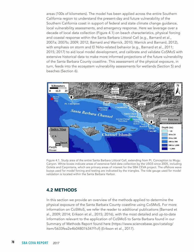
78 SBA CEVA REPORT 2017
areas (100s of kilometers). The model has been applied across the entire Southern California region to understand the present-day and future vulnerability of the Southern California coast in support of federal and state climate change guidance, local vulnerability assessments, and emergency response. Here we leverage over a decade of local data collection (Figure 4.1) on beach characteristics, physical forcing and coastal response within the Santa Barbara Littoral Cell (e.g., Barnard et al., 2007a; 2007b; 2009; 2012; Barnard and Warrick, 2010; Warrick and Barnard, 2012), with emphasis on storm and El Niño-related behavior (e.g., Barnard et al., 2011; 2015; 2017) to aid local model development, and calibrate and validate CoSMoS with extensive historical data to make more informed projections of the future vulnerability of the Santa Barbara County coastline. This assessment of the physical exposure, in turn, feeds into the ecosystem vulnerability assessments for wetlands (Section 5) and beaches (Section 6).
Figure 4.1. Study area of the entire Santa Barbara Littoral Cell, extending from Pt. Conception to Mugu Canyon. White boxes indicate areas of extensive field data collection by the USGS since 2005, including Goleta and Carpinteria, which are primary areas of interest for the SBA CEVA project. The offshore wave buoys used for model forcing and testing are indicated by the triangles. The tide gauge used for model validation is located within the Santa Barbara Harbor.
4.2 METHODS
In this section we provide an overview of the methods applied to determine the physical exposure of the Santa Barbara County coastline using CoSMoS. For more information on CoSMoS, we refer the reader to additional publications (Barnard et al., 2009; 2014; Erikson et al., 2015; 2016), with the most detailed and up-to-date information relevant to the application of CoSMoS to Santa Barbara found in our Summary of Methods Report found here (https://www.sciencebase.gov/catalog/item/5633fea2e4b048076347f1cf) (Erikson et al., 2017).
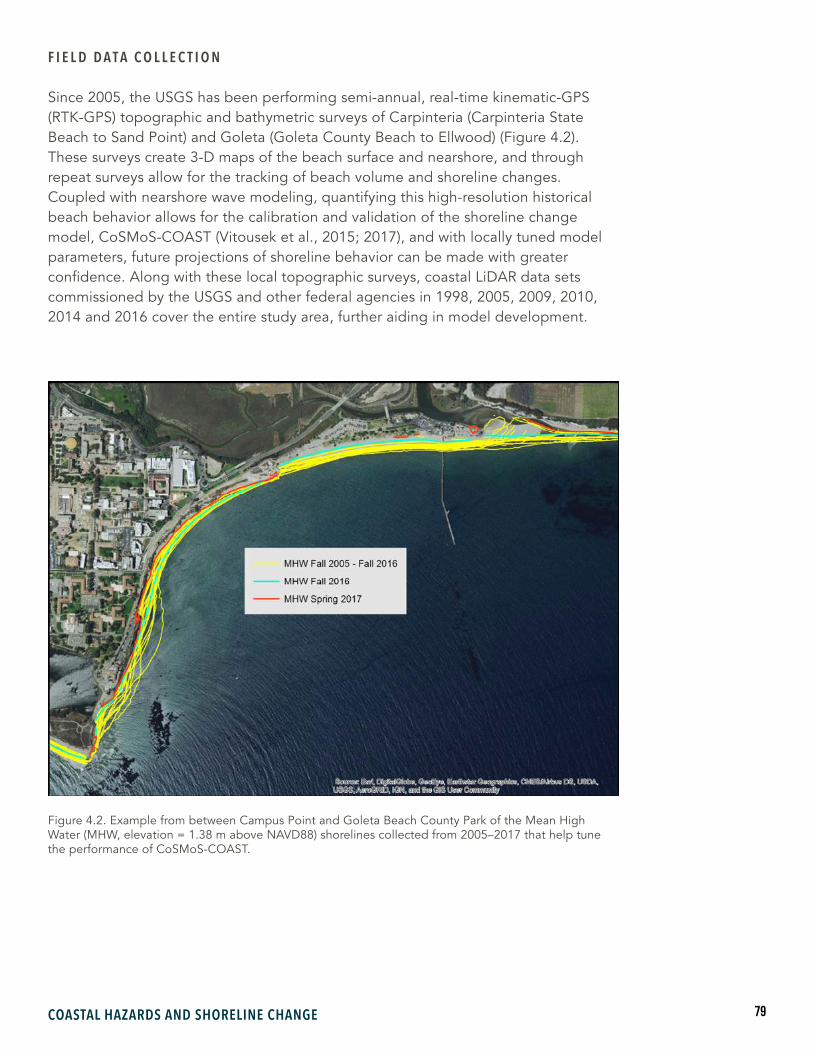
79COASTAL HAZARDS AND SHORELINE CHANGE
F I E L D D A T A C O L L E C T I O N
Since 2005, the USGS has been performing semi-annual, real-time kinematic-GPS (RTK-GPS) topographic and bathymetric surveys of Carpinteria (Carpinteria State Beach to Sand Point) and Goleta (Goleta County Beach to Ellwood) (Figure 4.2). These surveys create 3-D maps of the beach surface and nearshore, and through repeat surveys allow for the tracking of beach volume and shoreline changes. Coupled with nearshore wave modeling, quantifying this high-resolution historical beach behavior allows for the calibration and validation of the shoreline change model, CoSMoS-COAST (Vitousek et al., 2015; 2017), and with locally tuned model parameters, future projections of shoreline behavior can be made with greater confidence. Along with these local topographic surveys, coastal LiDAR data sets commissioned by the USGS and other federal agencies in 1998, 2005, 2009, 2010, 2014 and 2016 cover the entire study area, further aiding in model development.
Figure 4.2. Example from between Campus Point and Goleta Beach County Park of the Mean High Water (MHW, elevation = 1.38 m above NAVD88) shorelines collected from 2005–2017 that help tune the performance of CoSMoS-COAST.
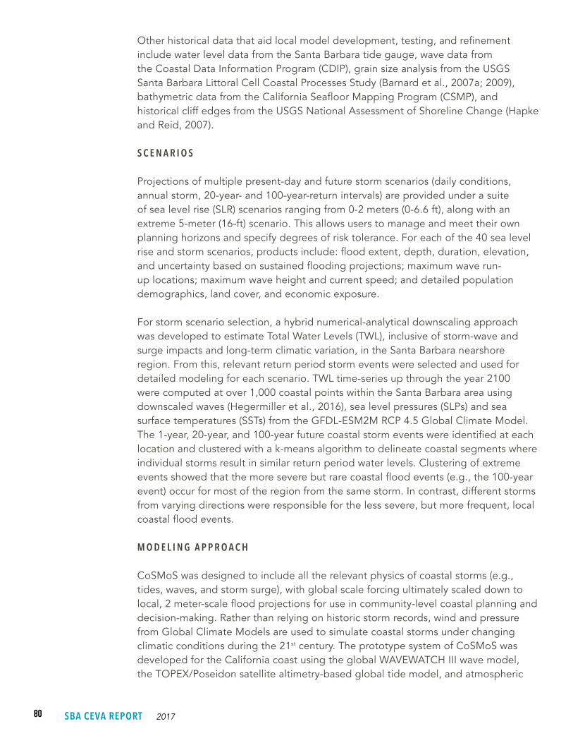
80 SBA CEVA REPORT 2017
Other historical data that aid local model development, testing, and refinement include water level data from the Santa Barbara tide gauge, wave data from the Coastal Data Information Program (CDIP), grain size analysis from the USGS Santa Barbara Littoral Cell Coastal Processes Study (Barnard et al., 2007a; 2009), bathymetric data from the California Seafloor Mapping Program (CSMP), and historical cliff edges from the USGS National Assessment of Shoreline Change (Hapke and Reid, 2007).
S C E N A R I O S
Projections of multiple present-day and future storm scenarios (daily conditions, annual storm, 20-year- and 100-year-return intervals) are provided under a suite of sea level rise (SLR) scenarios ranging from 0-2 meters (0-6.6 ft), along with an extreme 5-meter (16-ft) scenario. This allows users to manage and meet their own planning horizons and specify degrees of risk tolerance. For each of the 40 sea level rise and storm scenarios, products include: flood extent, depth, duration, elevation, and uncertainty based on sustained flooding projections; maximum wave run-up locations; maximum wave height and current speed; and detailed population demographics, land cover, and economic exposure.
For storm scenario selection, a hybrid numerical-analytical downscaling approach was developed to estimate Total Water Levels (TWL), inclusive of storm-wave and surge impacts and long-term climatic variation, in the Santa Barbara nearshore region. From this, relevant return period storm events were selected and used for detailed modeling for each scenario. TWL time-series up through the year 2100 were computed at over 1,000 coastal points within the Santa Barbara area using downscaled waves (Hegermiller et al., 2016), sea level pressures (SLPs) and sea surface temperatures (SSTs) from the GFDL-ESM2M RCP 4.5 Global Climate Model. The 1-year, 20-year, and 100-year future coastal storm events were identified at each location and clustered with a k-means algorithm to delineate coastal segments where individual storms result in similar return period water levels. Clustering of extreme events showed that the more severe but rare coastal flood events (e.g., the 100-year event) occur for most of the region from the same storm. In contrast, different storms from varying directions were responsible for the less severe, but more frequent, local coastal flood events.
M O D E L I N G A P P R O A C H
CoSMoS was designed to include all the relevant physics of coastal storms (e.g., tides, waves, and storm surge), with global scale forcing ultimately scaled down to local, 2 meter-scale flood projections for use in community-level coastal planning and decision-making. Rather than relying on historic storm records, wind and pressure from Global Climate Models are used to simulate coastal storms under changing climatic conditions during the 21st century. The prototype system of CoSMoS was developed for the California coast using the global WAVEWATCH III wave model, the TOPEX/Poseidon satellite altimetry-based global tide model, and atmospheric
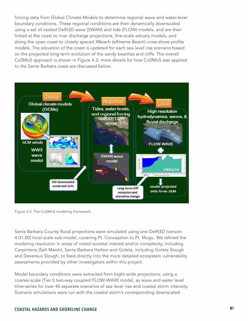
81COASTAL HAZARDS AND SHORELINE CHANGE
forcing data from Global Climate Models to determine regional wave and water-level boundary conditions. These regional conditions are then dynamically downscaled using a set of nested Delft3D wave (SWAN) and tide (FLOW) models, and are then linked at the coast to river discharge projections, fine-scale estuary models, and along the open coast to closely spaced XBeach (eXtreme Beach) cross-shore profile models. The elevation of the coast is updated for each sea level rise scenario based on the projected long-term evolution of the sandy beaches and cliffs. The overall CoSMoS approach is shown in Figure 4.3; more details for how CoSMoS was applied to the Santa Barbara coast are discussed below.
Santa Barbara County flood projections were simulated using one Delft3D (version 4.01.00) local-scale sub-model, covering Pt. Conception to Pt. Mugu. We refined the modeling resolution in areas of noted societal interest and/or complexity, including Carpinteria (Salt Marsh), Santa Barbara Harbor and Goleta, including Goleta Slough and Devereux Slough, to feed directly into the more detailed ecosystem vulnerability assessments provided by other investigators within this project.
Model boundary conditions were extracted from bight-wide projections, using a coarser-scale (Tier I) two-way coupled FLOW-WAVE model, as wave and water level time-series for over 40 separate scenarios of sea level rise and coastal storm intensity. Scenario simulations were run with the coastal storm’s corresponding downscaled
Figure 4.3. The CoSMoS modeling framework.
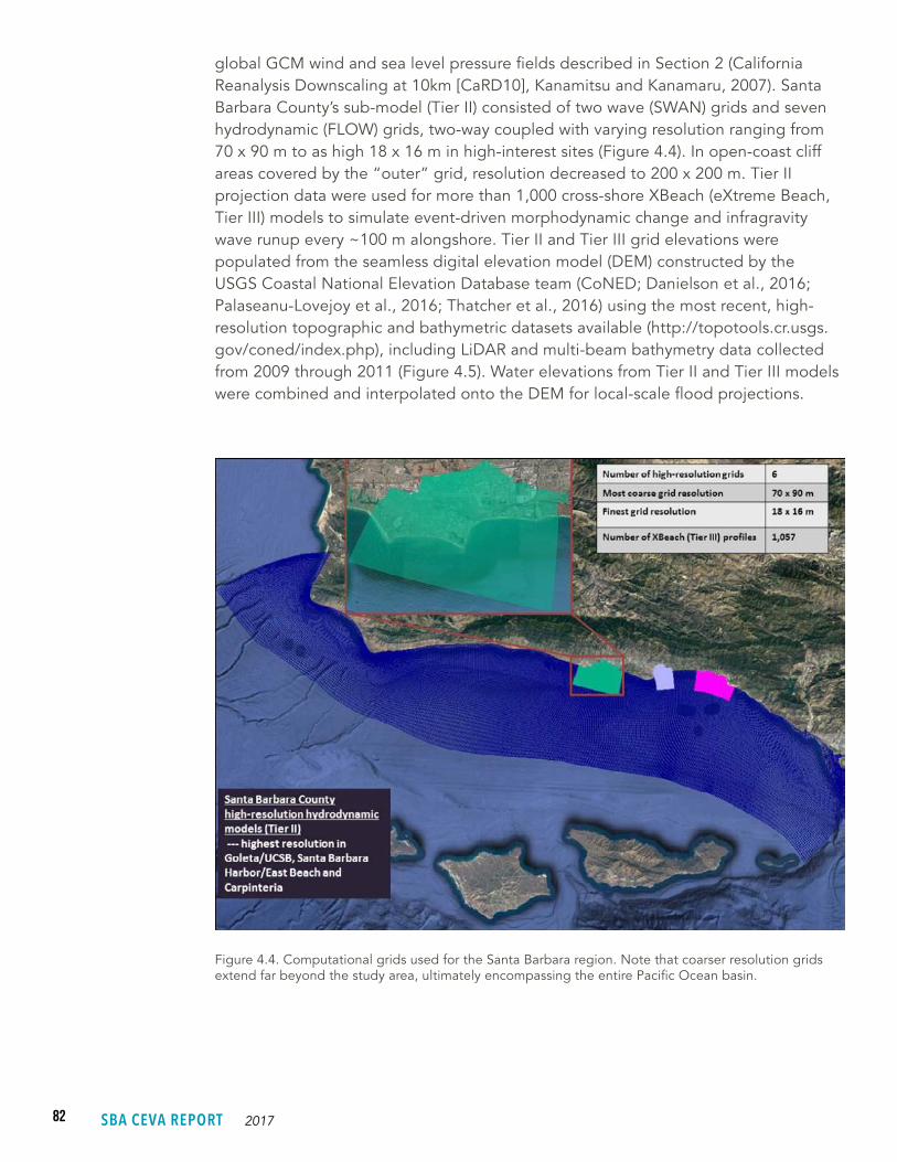
82 SBA CEVA REPORT 2017
global GCM wind and sea level pressure fields described in Section 2 (California Reanalysis Downscaling at 10km [CaRD10], Kanamitsu and Kanamaru, 2007). Santa Barbara County’s sub-model (Tier II) consisted of two wave (SWAN) grids and seven hydrodynamic (FLOW) grids, two-way coupled with varying resolution ranging from 70 x 90 m to as high 18 x 16 m in high-interest sites (Figure 4.4). In open-coast cliff areas covered by the “outer” grid, resolution decreased to 200 x 200 m. Tier II projection data were used for more than 1,000 cross-shore XBeach (eXtreme Beach, Tier III) models to simulate event-driven morphodynamic change and infragravity wave runup every ~100 m alongshore. Tier II and Tier III grid elevations were populated from the seamless digital elevation model (DEM) constructed by the USGS Coastal National Elevation Database team (CoNED; Danielson et al., 2016; Palaseanu-Lovejoy et al., 2016; Thatcher et al., 2016) using the most recent, high-resolution topographic and bathymetric datasets available (http://topotools.cr.usgs.gov/coned/index.php), including LiDAR and multi-beam bathymetry data collected from 2009 through 2011 (Figure 4.5). Water elevations from Tier II and Tier III models were combined and interpolated onto the DEM for local-scale flood projections.
Figure 4.4. Computational grids used for the Santa Barbara region. Note that coarser resolution grids extend far beyond the study area, ultimately encompassing the entire Pacific Ocean basin.

83COASTAL HAZARDS AND SHORELINE CHANGE
Long-term shoreline change and cliff retreat projections also are provided, including uncertainty, using state-of-the-art approaches for each of the 10 sea level rise scenarios. In addition, multiple management scenarios are provided for each of these long-term projections of coastal change, where we assume historical rates of beach nourishment continue into the future (or not) and/or where we assume no erosion beyond existing urban infrastructure (or not), i.e., “hold the line.” For the integration of coastal change with the flooding projections, we assume no further nourishment will occur but that local communities will “hold the line” at the current urban interface.
Figure 4.5. Seamless, 2-m resolution DEM for the Goleta region.
84 SBA CEVA REPORT 2017
Figure 4.6. CoSMoS-COAST model domain for Santa Barbara County. Green transects indicate long sandy beaches; yellow transects represent short sandy (“pocket”) beaches; red transects represent mixed sandy/rocky beaches; and black transects represent harbors and armored or cliffed beaches. Future shoreline projections are shown for Santa Barbara Harbor and Carpinteria.
Predictions of sandy shoreline change for Santa Barbara County (Figure 4.6) were produced by CoSMoS-COAST (Coastal One-line Assimilated Simulation Tool; Vitousek et al., 2017). The model accounts for the dynamical processes of wave-driven alongshore and cross-shore transport, shoreline retreat due to scenarios of sea level rise (Figure 4.7), and natural and anthropogenic sources of sediment estimated via data assimilation of historical shoreline data. The model is “trained” with historical wave and shoreline data through 2010, and the calibrated model is used to produce a prediction of shoreline evolution by 2100. Historical shoreline data in Santa Barbara comes from 3 aerial LiDAR surveys (fall 1997, spring 1998, and fall 2009), as well as semi-annual USGS GPS surveys conducted in Goleta and Carpinteria since 2005.
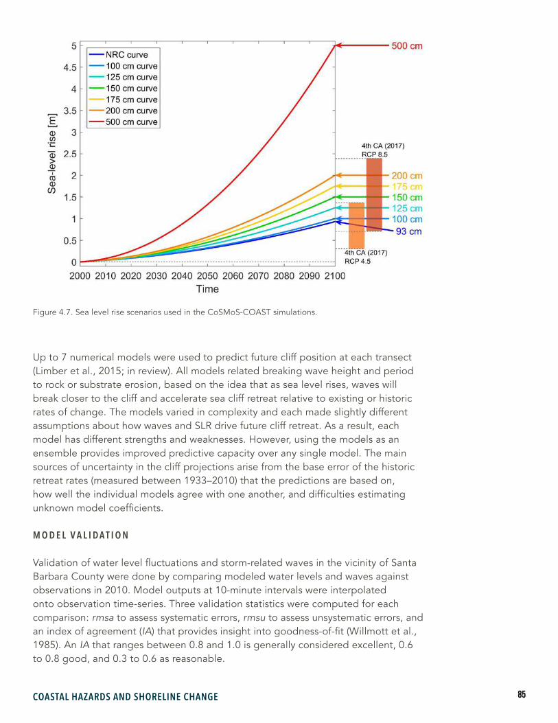
85COASTAL HAZARDS AND SHORELINE CHANGE
Up to 7 numerical models were used to predict future cliff position at each transect (Limber et al., 2015; in review). All models related breaking wave height and period to rock or substrate erosion, based on the idea that as sea level rises, waves will break closer to the cliff and accelerate sea cliff retreat relative to existing or historic rates of change. The models varied in complexity and each made slightly different assumptions about how waves and SLR drive future cliff retreat. As a result, each model has different strengths and weaknesses. However, using the models as an ensemble provides improved predictive capacity over any single model. The main sources of uncertainty in the cliff projections arise from the base error of the historic retreat rates (measured between 1933–2010) that the predictions are based on, how well the individual models agree with one another, and difficulties estimating unknown model coefficients.
M O D E L V A L I D A T I O N
Validation of water level fluctuations and storm-related waves in the vicinity of Santa Barbara County were done by comparing modeled water levels and waves against observations in 2010. Model outputs at 10-minute intervals were interpolated onto observation time-series. Three validation statistics were computed for each comparison: rmsa to assess systematic errors, rmsu to assess unsystematic errors, and an index of agreement (IA) that provides insight into goodness-of-fit (Willmott et al., 1985). An IA that ranges between 0.8 and 1.0 is generally considered excellent, 0.6 to 0.8 good, and 0.3 to 0.6 as reasonable.
Figure 4.7. Sea level rise scenarios used in the CoSMoS-COAST simulations.

86 SBA CEVA REPORT 2017
A model hindcast of tides, with no storm, was simulated for October and November, 2010. This is the time-period that was used to represent a spring tide (i.e., maximum monthly tides that occur during full and new moon) in all CoSMoS scenario runs. Modeled tidal fluctuations compare well to predicted tides at the Santa Barbara gauge (NOAA) as shown in Figure 4.8A and 4.8B. Peaks are slightly over-predicted resulting in a systematic error of about 5 cm (Figure 4.8B), but overall the agreement is excellent with an IA of 0.99.
To assess the ability of the model to accurately simulate storm surges and other non-tidal water level fluctuations, the storm of January 2010 was hindcast. Measurements at the Harvest (CDIP071), San Nicolas Island (CDIP067), and East Santa Barbara (NDCB46053) buoys, located in deep water offshore of Santa Barbara County, indicate that strong sustained winds in excess of 12 m/s (minimum sea level pressures ~1010hPa) were accompanied by high waves in excess of 7 m. The storm event was simulated by applying time- and space-varying CaRD10 (Kanamaru and Kanamitsu, 2007) wind and sea level pressure fields across all model grids and deep water swell observed at buoy CDIP067 along the open boundaries of the Tier1 model grid. Model results compare well with observations at the Santa Barbara tide gauge (rmsa = 0.04 m; rmsu = 0.08 m; and IA = 0.99) where water levels were measured to be >0.3 m above normal astronomic tides (Figures 4.8C-D).
Modeled wave statistics were compared to observations at the CDIP111 buoy to evaluate the ability of the model to replicate waves in the nearshore region. Results from the same January 2010 storm are used for comparison. Measurements indicate a substantial decrease in wave energy from the offshore deep waters, likely due to refraction around and partial shadowing by the Channel Islands. Maximum measured wave heights were slightly lower at 2.96 m compared to maximum modeled wave heights of 3.26 m, an over-prediction of 0.30 m, commensurate with the rmsa and rmsu (0.32 m and 0.27 m, respectively, Figure 4.8E). Whereas the maximum wave heights are somewhat over-predicted, the overall skill is good with an IA of 0.85. The mean wave period and incident wave directions are less well represented but are reasonable to good with IA values of 0.50 and 0.69, respectively (Figures 4.8F-G). Previous studies have also found that modeling waves in the nearshore region of Santa Barbara (especially Santa Barbara Channel) is notoriously difficult (e.g., O’Reilly et al., 2016).
4.3 RESULTS/DISCUSSION
C O A S T A L F L O O D I N G
CoSMoS flooding projections indicate serious concerns in the Santa Barbara region over the coming decades, including areas comprising sensitive coastal ecosystems, such as the region’s coastal estuaries and creeks, narrow, often bluff-backed beaches, and dune fields. The most vulnerable regions for future flooding include Carpinteria, Santa Barbara Harbor/East Beach, Goleta Slough/Santa Barbara Airport, Devereux Slough and Gaviota State Park (Figure 4.9). Several of these locations, such as Goleta

87COASTAL HAZARDS AND SHORELINE CHANGE
Figure 4.8. Time-series and scatter plots comparing modeled water levels and wave statistics with measurements in the vicinity of Santa Barbara County. A-B) Modeled water levels and deterministically predicted astronomic tides for ~16 days in October and November 2010. C-D) Modeled water levels compared to predicted tides and measurements that include storm surge and other non-tidal water level components (black solid line) during a storm in January 2010. Scatter plot in D compares modeled water levels to measured water levels that deviate at least ± 5 cm from predicted tides. E-G) Comparison of modeled and measured significant wave heights, mean wave periods, and peak incident wave directions at CDIP buoy 111 for the same storm event as in C and D.
Slough/Santa Barbara Airport and Carpinteria, are vulnerable to coastal flooding from a major storm at present, while the vulnerability of other locations is more acute later in the century. The East Beach area, for example, doesn’t reach a tipping point for extreme storm impacts until between 0.5 and 1 m of SLR (Box 4), expected between the middle and the end of the century; exposure to flooding then increases progressively through the higher SLR scenarios. Conversely, the projected flooding for Carpinteria during an extreme storm, including the salt marsh and state park, already is very high today, but doesn’t begin to increase appreciably until higher SLR scenarios are reached (e.g., 1.5 m). Goleta Slough and Carpinteria Salt Marsh (see also Section 5), in addition to the region’s many narrow beaches (see also Section 6) and small creek mouths, would be extremely vulnerable to everyday flooding independent of storm conditions for SLR scenarios expected later this century (i.e., 0.5 to 1 m), indicating a complete displacement of existing ecosystems.

88 SBA CEVA REPORT 2017
Figure 4.9. Example of future flood hazards in Goleta (top), Santa Barbara Harbor/East Beach (middle) and Carpinteria (bottom), showing the 1-m SLR scenario coupled with the 100-year coastal storm. See Sections 5 and 6 for salt marsh and beach ecosystem impacts.

89COASTAL HAZARDS AND SHORELINE CHANGE
B E A C H C H A N G E S
The model predictions (Figures 4.10-11) for Santa Barbara County estimate that shorelines will erode by more than 25 m by 2100 (Figure 4.10) without large-scale human interventions. But more importantly, given that beaches across this region are often backed by resistant cliffs or immobile urban infrastructure, many beaches will narrow considerably and 50 to 75% of the beaches may experience complete erosion (up to infrastructure or cliffs) by 2100 (Figure 4.11). The narrowing and/or loss of future beaches (and the ecosystems supported by those beaches–see Section 6) will primarily result from accelerating SLR combined with a lack of ample sediment in the system, which together will continue to drive the landward erosion of beaches, effectively drowning them between the rising ocean and the backing cliffs and/or urban hardscape. The beaches along the UCSB shoreline, for example, are almost completely devoid of dry sand at high tide today. This both stresses existing sandy beach ecosystems and leaves the cliffs more vulnerable to wave attack, placing cliff top ecosystems and structures at increased risk.
Figure 4.10. Average beach loss in Santa Barbara County by by 2050 (left) and 2100 (right) under the sea level rise scenarios given in Figure 4.7. The four management scenarios are: (1) Existing armoring maintained (a.k.a. “hold the line”) + no future nourishment (2) Existing armoring maintained + future nourishment, (3) Ignore existing coastal armoring + no future nourishment, and (4) Ignore existing coastal armoring + inclusion of future nourishment. There is very little difference between scenarios 1 and 2 because historical rates of beach nourishment in Santa Barbara County are extremely low.
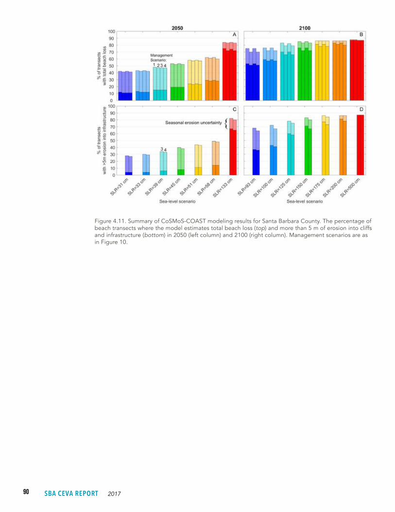
90 SBA CEVA REPORT 2017
Figure 4.11. Summary of CoSMoS-COAST modeling results for Santa Barbara County. The percentage of beach transects where the model estimates total beach loss (top) and more than 5 m of erosion into cliffs and infrastructure (bottom) in 2050 (left column) and 2100 (right column). Management scenarios are as in Figure 10.

91COASTAL HAZARDS AND SHORELINE CHANGE
C L I F F R E T R E A T
Mean historical cliff retreat rates across Santa Barbara average ~0.2 m/yr. Model results suggest that a 1-m rise in sea level will accelerate retreat rates to 0.31 m/yr during the 21st century, an increase of 55%. In addition to the threat to cliff-toe and cliff-top ecosystems throughout the region, cliff retreat will also be a serious threat to sections of Highway 101 and the Union Pacific Railroad corridor over the coming century, particularly in the western portions of the study area (i.e., toward Gaviota) and Summerland, in addition to residential and undeveloped property in Isla Vista, More Mesa and the Santa Barbara Mesa.
Figure 4.12. Example of cliff retreat hazards between Goleta County Beach and Campus Point. Colored bands around the lines represent projection uncertainty for that sea level rise scenario.

BOX 3
LAND COVER AND SOCIOECONOMIC IMPACTS
The coastal flood hazard projections for each of the four storm scenarios and the SLR rise scenarios from 0 to 2 m were translated into socioeconomic impacts (Jones et al., 2016), and can be viewed interactively on the Hazard Exposure Reporting and Analytics (HERA) website (https://geography.wr.usgs.gov/science/vulnerability/HERA.html). A couple of noteworthy items are discussed below and select scenarios are summarized in Table B1.
The proportion of coastal flooding affecting developed vs. undeveloped land is roughly equivalent across scenarios, with wetlands and open space generally being most vulnerable to present-day and future coastal flooding among the undeveloped land cover types. However, the undeveloped flooded areas that are designated as shrubs/grassland and
Table B1. Summary of land cover and socioeconomic exposure to flooding for select SLR (0-2m) and storm scenarios.
open space increase the most as SLR increases. While the area of wetland flooding doesn’t change significantly, wetland habitat is projected to change dramatically by mid-century (Section 5). Overall, there is little change in flooding exposure when transitioning from the 0 to 0.5 m SLR scenarios, but there is a significant change from 0.5 to 1 m, particularly for the no-storm scenarios, and another significant change from 1 to 2 m SLR for the 100-year storm scenarios. In almost all cases extreme storms significantly increase the areas exposed to flooding, especially for the 0.5 and 2 m SLR scenarios, where land area exposed to flooding can more than double during storms compared to SLR alone.
Extreme storms can more than triple the number of residents and parcel values exposed in Santa Barbara County when compared to the no-storm scenarios (e.g., 0.5 m SLR). Further, a 1 m SLR scenario (~mid-range SLR projection by 2100) combined with a 100-year storm could
expose more than 4,000 people to flooding along with more than $800 million in property, but for an upper end SLR scenario by 2100 (i.e., 2 m of SLR), the population and parcel values exposed to flooding during an extreme storm will triple to almost 12,000 residents and ~$2.4 billion, respectively (for Santa Barbara County residents from Point Conception to the Ventura County line). There is also a notable ~3 fold-increase for both residents and parcel value exposure when comparing the 0.5 and 1 m SLR/no-storm scenarios. In summary, storms and the higher-end SLR scenarios (i.e., 0.5 m+) expected in the latter half of the century pose the greatest risk to ecosystems, population, and the economy of the region.
93COASTAL HAZARDS AND SHORELINE CHANGE
4.4 KEY FINDINGS
• The most vulnerable regions for future flooding across the region include Carpinteria, East Beach, Santa Barbara Airport/Goleta Slough, Devereux Slough, and Gaviota State Park, but also the area’s many narrow, bluff-backed beaches and small creek mouths.
• Certain areas are extremely vulnerable to present-day coastal flooding from an extreme storm, such as Carpinteria and Santa Barbara Airport/Goleta Slough, while in other areas, such as East Beach, the vulnerability doesn’t increase significantly until ~1 m of SLR.
• There is a clear tipping point between ~0.5 and 1 m of SLR where overall vulnerability increases across the region, especially for the no-storm scenarios, which indicate the potential for permanent inundation later this century in some important areas (e.g., Carpinteria and Santa Barbara Airport/Goleta Slough).
• Many beaches will narrow considerably and as many as 75% could be completely lost over the next century as the beaches are squeezed between the rising seas and backing cliffs or urban infrastructure.
• Cliff retreat will increasingly pose a significant hazard across the region, as SLR could increase retreat rates by ~55% over historical rates.
• Up to ~10 km2 of undeveloped land in the study area could be exposed to flooding over the next century, with wetlands, shrubs/grassland and open space being the most extensively flooded land cover types.
• Over 12,000 people and $2.4 billion in property are at risk of coastal flooding over the next century for upper end SLR scenarios under extreme storm conditions, but there is significant risk today, with ~$0.5 billion in property exposed to the 100-year coastal storm.
• In almost every instance, extreme storms significantly increase the flooding exposure and potential impacts to coastal ecosystems, residents and property, when compared to SLR alone.
While these conclusions may seem dire or insurmountable, the threat of frequent flooding, permanent inundation, and beach loss doesn’t increase significantly until at least 0.5 m of SLR (~2050), so there may be some time, based on current SLR projections, to design and implement suitable coastal management actions to mitigate future impacts. It should be noted, however, that significant changes to the wetland habitats (Section 5) and beach ecology (Section 6) are already well underway upon reaching 0.5 m of SLR, due in part to limits on habitat migration
94 SBA CEVA REPORT 2017
hampered by the bordering cliffs and surrounding urban environment. Further, new SLR research on the instability of the West Antarctic Ice Sheet (e.g., DeConto and Pollard, 2016) suggests the possibility that up to ~3 m of SLR may be possible by 2100, and the state of California is considering adding such an extreme SLR scenario to their updated guidance (Griggs et al., 2017). By comparison, current state guidance suggests that 1.67 m is the upper end of the potential SLR range by 2100 (Nation Research Council, 2012). Regardless of the SLR curve, applying effective sediment management practices will be a key factor in preserving the region’s coastal ecosystems and mitigating future coastal hazards. Sand is a valuable resource, especially for a sediment-starved stretch of coastline like southern Santa Barbara County, so keeping existing sand in the system and adding as much sand as possible to beaches will be a key component of future coastal management efforts to maintain beach widths, healthy ecosystems, and to protect adjacent communities from flooding. However, in some highly vulnerable areas, the most pragmatic action might be to retreat from the coastline, but these kinds of difficult decisions can only be made after careful and extensive community-based discussions on the vision for the Santa Barbara coastline.
Aaron H
oward
95ESTUARIES
5. EstuariesAUTHORS: HENRY M. PAGE, BRANDON DOHENY, JUSTIN HOESTEREY, RUSSELL JOHNSTON, DAVID M. HUBBARD, STEPHEN C. SCHROETER, MONIQUE R. MYERS
5.1 INTRODUCTION
California has lost more than 90% of wetland habitat over the past 200 years with the remainder altered and threatened by human activities and climate change (Dahl, 1990; Zedler, 2004; Grewell et al., 2007). Since about 1850, there has been a 48% loss of California estuarine wetlands within the Southern California Bight (SCB) with an even greater loss (62%) in Santa Barbara County (Stein et al., 2014). These estuarine wetlands are vulnerable to increasing rates of sea level rise (SLR) that will likely exceed the 20th century observed rate, and which by some scenarios could exceed one meter or more by the end of the 21st century (NRC, 2012, Section 2 this volume). The effects of climate change and the impacts of sea level rise on coastal
Aaron H
oward
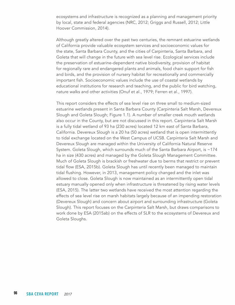
96 SBA CEVA REPORT 2017
ecosystems and infrastructure is recognized as a planning and management priority by local, state and federal agencies (NRC, 2012; Griggs and Russell, 2012; Little Hoover Commission, 2014).
Although greatly altered over the past two centuries, the remnant estuarine wetlands of California provide valuable ecosystem services and socioeconomic values for the state, Santa Barbara County, and the cities of Carpinteria, Santa Barbara, and Goleta that will change in the future with sea level rise. Ecological services include the preservation of estuarine-dependent native biodiversity, provision of habitat for regionally rare and endangered plants and animals, food chain support for fish and birds, and the provision of nursery habitat for recreationally and commercially important fish. Socioeconomic values include the use of coastal wetlands by educational institutions for research and teaching, and the public for bird watching, nature walks and other activities (Onuf et al., 1979; Ferren et al., 1997).
This report considers the effects of sea level rise on three small to medium-sized estuarine wetlands present in Santa Barbara County (Carpinteria Salt Marsh, Devereux Slough and Goleta Slough; Figure 1.1). A number of smaller creek mouth wetlands also occur in the County, but are not discussed in this report. Carpinteria Salt Marsh is a fully tidal wetland of 93 ha (230 acres) located 12 km east of Santa Barbara, California. Devereux Slough is a 20 ha (50 acres) wetland that is open intermittently to tidal exchange located on the West Campus of UCSB. Carpinteria Salt Marsh and Devereux Slough are managed within the University of California Natural Reserve System. Goleta Slough, which surrounds much of the Santa Barbara Airport, is ~174 ha in size (430 acres) and managed by the Goleta Slough Management Committee. Much of Goleta Slough is brackish or freshwater due to berms that restrict or prevent tidal flow (ESA, 2015b). Goleta Slough has until recently been managed to maintain tidal flushing. However, in 2013, management policy changed and the inlet was allowed to close. Goleta Slough is now maintained as an intermittently open tidal estuary manually opened only when infrastructure is threatened by rising water levels (ESA, 2015). The latter two wetlands have received the most attention regarding the effects of sea level rise on marsh habitats largely because of an impending restoration (Devereux Slough) and concern about airport and surrounding infrastructure (Goleta Slough). This report focuses on the Carpinteria Salt Marsh, but draws comparisons to work done by ESA (2015ab) on the effects of SLR to the ecosystems of Devereux and Goleta Sloughs.

97ESTUARIES
S E C T I O N O B J E C T I V E S
• Explore how expected SLR will affect the habitats and biological communities of Santa Barbara County estuaries with a focus on Carpinteria Salt Marsh.
• Discuss factors affecting the potential timing of habitat evolution in the face of SLR.
• Compare projected effects of SLR on marsh habitats to those observed during a short-term positive sea level anomaly associated with the El Niño of 2015–2016.
• Identify monitoring data that could inform the timing of adaptation measures to ameliorate the effects of SLR on estuarine habitats and resources.
Figure 5.1. Location of Carpinteria Salt Marsh outlined in red.

98 SBA CEVA REPORT 2017
5.2 METHODS
S T U D Y S I T E – C A R P I N T E R I A S A L T M A R S H
The physical and biological features of Carpinteria Salt Marsh (34° 24’04. 48”N, 119° 32’16.60”W) are described in Ferren (1985), Page et al. (1995), Hubbard (1996), Ferren et al. (1997), and Sadro et al. (2007). Briefly, the wetland is a geomorphologically mature system that drains almost completely at tides lower than ~0.5 m (~1.5’) NAVD88. The regularly flooded middle tidal marsh is vegetated primarily by a salt tolerant succulent, pickleweed, Sarcocornia pacifica (=Salicornia virginica). Other species, including the succulents Arthrocnemum subterminale and Jaumea carnosa, salt grass Distichlis spicata, and alkali heath Frankenia salina, are found along with Sarcocornia at higher tidal elevations. Cordgrass, Spartina foliosa, and the subtidal eelgrass, Zostera marina, present in some other larger Southern California marshes (e.g., Tijuana Estuary; Zedler et al., 1992), are absent.
The climate of Southern California is Mediterranean, characterized by intense, intermittent rainfall during the winter months with seasonal drought during the summer and fall. Most precipitation (80%) and freshwater runoff occurs between the months of December and March (Beighley et al., 2005). Runoff originating from mountainous watersheds and the coastal plain enters Carpinteria Salt Marsh primarily in two larger streams (Santa Monica Creek, Franklin Creek) in the eastern portion of the wetland (Figure 5.1). Four smaller drainages also convey runoff from the coastal plain into the western half of the wetland (Page et al., 1995). The two larger streams are channelized, which reduces contact of these waters with the marsh plain (Page et al., 1995; Sadro et al., 2007). Runoff volume is highly variable with maximum discharge coinciding with seasonal storm events. Tidal waters from the Santa Barbara Channel enter the wetland through an inlet at the southern border maintained open through a rock revetment constructed in 1966 (Figure 5.1). The wetland is surrounded by urban and residential development that includes railroad tracks, roads, housing and business development (Page et al., 1995; Ferren et al., 1997).
S E A L E V E L R I S E S C E N A R I O S
Estimates of the timing and extent of sea level rise vary with the model used to make these predictions. In our analysis, we used regional sea level rise scenarios from the National Research Council (NRC, 2012), which include a possible sea level rise of up to 167 cm (66 in) by the year 2100 (Table 5.1, Figure 5.2). The NRC (2012) models incorporate an estimate of regional subsidence of 1.5 mm per year. This subsidence rate is similar to that estimated recently (1.2 mm per year) for the Carpinteria Salt Marsh area by Simms et al. (2016). Uncertainty in the rate of sea level rise increases with time, such that the difference between low and high scenarios increases from 25.4 cm by the year 2030 to 122.3 cm (6.7 to 48.1 inches) by 2100 (Table 5.1, Figure 5.2). To accommodate this uncertainty, we estimated habitat change associated with
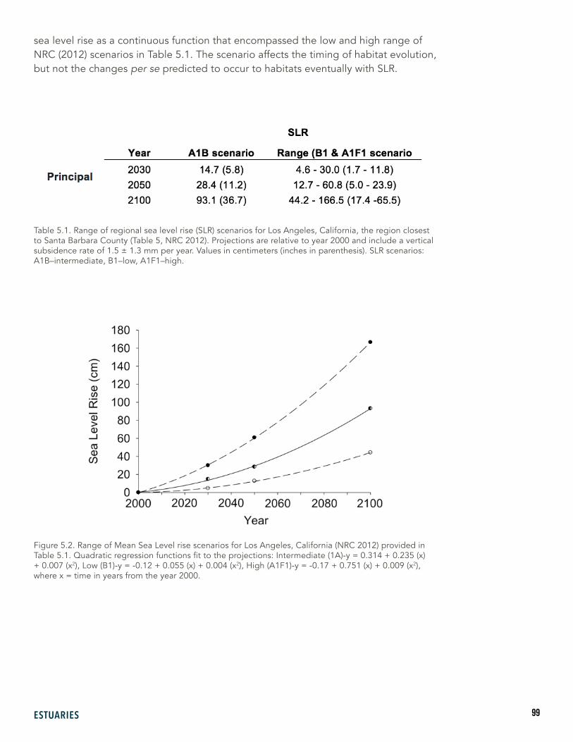
99ESTUARIES
Table 5.1. Range of regional sea level rise (SLR) scenarios for Los Angeles, California, the region closest to Santa Barbara County (Table 5, NRC 2012). Projections are relative to year 2000 and include a vertical subsidence rate of 1.5 ± 1.3 mm per year. Values in centimeters (inches in parenthesis). SLR scenarios: A1B–intermediate, B1–low, A1F1–high.
Figure 5.2. Range of Mean Sea Level rise scenarios for Los Angeles, California (NRC 2012) provided in Table 5.1. Quadratic regression functions fit to the projections: Intermediate (1A)-y = 0.314 + 0.235 (x) + 0.007 (x2), Low (B1)-y = -0.12 + 0.055 (x) + 0.004 (x2), High (A1F1)-y = -0.17 + 0.751 (x) + 0.009 (x2), where x = time in years from the year 2000.
sea level rise as a continuous function that encompassed the low and high range of NRC (2012) scenarios in Table 5.1. The scenario affects the timing of habitat evolution, but not the changes per se predicted to occur to habitats eventually with SLR.
100 SBA CEVA REPORT 2017
W E T L A N D H A B I T A T C A T E G O R I E S
A map of the distribution and area of existing habitats in Carpinteria Salt Marsh was created from a multispectral aerial image acquired by Ocean Imaging (Littleton, CO) on May 27, 2013 using a Microsoft UltraCam-X digital camera recording in the red, green, blue and near-infrared bands. The camera was flown by fixed wing aircraft and achieved a resolution (pixel size) on the ground of 20 cm. The acquired image was geo-referenced to within one meter of fixed reference points. Vegetation classification algorithms were run on the assembled image to produce a preliminary vegetation/habitat classification.
We combined the preliminary vegetation/habitat classifications into broader, simplified estuarine wetland habitats (Figure 5.3a) based on general vegetation composition and elevation similar to that done in a management and sea level rise plan for Goleta Slough (ESA 2015b). The habitats and grouping criteria consisted of: 1) open water subtidal–continuously submerged with regular tidal exchange, <0.4 m NAVD88, 2) mudflat–unvegetated with regular tidal inundation, further divided into high mudflat (frequently exposed, inundated <50% of the time) and low mudflat (frequently flooded, inundated ≥ 50% of the time—both categories include pixels scored as algae that occurred on mudflat), 3) coastal salt marsh–vegetated by halophytic plants, further divided into middle and high marsh on the basis of general plant species composition, with S. pacifica dominant in the middle marsh at lower elevations, and a mixture of species, including S. pacifica, Arthrocnemum subterminale, Frankenia salina, and Distichlis spicata, at the higher elevations, 4) salt panne–sparsely vegetated and characterized by hypersaline soils at higher elevations, 5) salt marsh–upland transition habitat that encompasses a gradient from salt marsh to terrestrial vegetation infrequently hit by the tides. At Carpinteria Salt Marsh, regionally rare and endangered species that include Cordylandthus maritimus (=Chloropyron maritimum), Lasthenia glabrata, Sueda calceoliformis, and Astragalus pycnostachyus var. lanosissimus (introduced by USFWS in 2002), along with high marsh species are found in this habitat (Ferren, 1985), and 6) undeveloped upland, which is limited within the boundaries of the Carpinteria Salt Marsh area of interest due to surrounding residential and commercial development. This habitat is largely vegetated by non-native shrubs (e.g., Myoporum laetum) and grasses (e.g., Lolium mulitflorum, Bromus diandrus) (Ferren, 1985).
Pacific cordgrass, Spartina foliosa, which occurs at and below the intertidal distribution of Sarcocornia, is considered characteristic of “low” salt marsh (Zedler et al., 1992). There is no historical evidence for the occurrence of cordgrass in Carpinteria Salt Marsh or other coastal wetlands in Santa Barbara County. Nevertheless, portions of high mudflat in Carpinteria occur within an inundation environment that supports cordgrass in other wetlands of Southern California (Table 5.2). Since cordgrass could colonize in the future, we include habitat evolution scenarios with low marsh habitat, depicting the extent to which the inundation regime could favor cordgrass establishment.
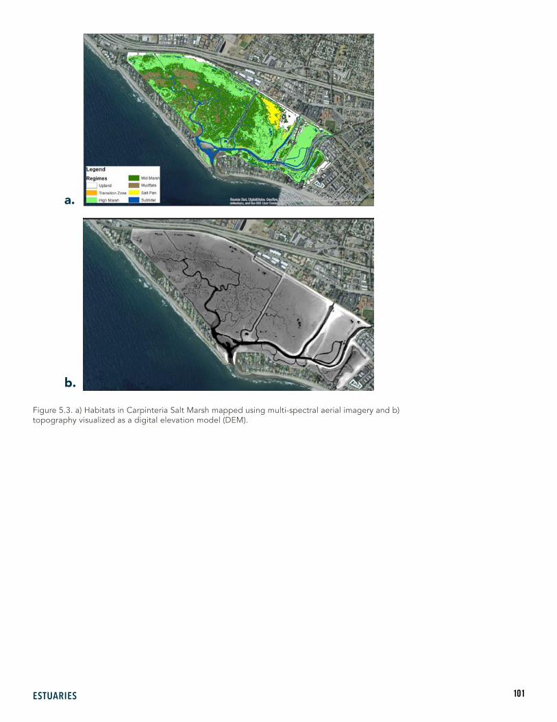
101ESTUARIES
Figure 5.3. a) Habitats in Carpinteria Salt Marsh mapped using multi-spectral aerial imagery and b) topography visualized as a digital elevation model (DEM).
a.
b.

102 SBA CEVA REPORT 2017
Seepage of freshwater along the northern border of the marsh has enabled the establishment of a small area (~1000 m2) of “brackish” marsh habitat vegetated by cattail, Typha domingensis, and bulrush, Scirpus (Bolboschenus) maritimus, in previous years. With four years of drought and reduced freshwater intrusion, this habitat had disappeared and was not included in our analysis.
T O P O G R A P H Y A N D H A B I T A T D I S T R I B U T I O N S
We linked elevation (as NAVD88) and habitat distributions (based on vegetation) using a digital elevation model (DEM) constructed from data acquired by the California Coastal Conservancy Coastal Light Detection and Ranging (LiDAR) Project (https://coast.noaa.gov/dataviewer/index.html?action=advsearch&qType=in&qFld=ID&qVal=1124#) (Figure 5.3b). LiDAR data collection was performed using a Leica ALS60 MPiA sensor deployed on fixed winged aircraft between October 2009 and August 2011. All geospatial modeling of topography and habitat distributions was done in Model Builder using ArcGIS 10.3. The DEM and vegetation layer datasets differed in their projection, resolution, extent and alignment. For the analysis, all datasets were first converted to an appropriate projection (WGS_1984_UTM_Zone_11N), a pixel size of 2 m, and combined following alignment.
LiDAR DEMs overestimate actual elevations in vegetated areas (Sadro et al., 2007). We evaluated this source of error in our study by comparing geo-referenced LiDAR DEM elevations with data collected using a network Spectra Precision real time kinematic (RTK) global positioning system interfaced with a SP80 receiver and a Juno T41 data collector. Elevations and in situ measurements of vegetation height were measured at 2114 points distributed along habitat transitions and transects across habitats. We found discrepancies of up to +31 cm between the LiDAR and RTK elevations presumably caused by vegetation canopy within specific habitat types. The LiDAR elevations for the habitats of interest within the DEM were adjusted downward using average RTK elevations for each habitat type.
H A B I T A T E V O L U T I O N M O D E L
To evaluate the vulnerability of Carpinteria Salt Marsh habitats to SLR, we developed a conceptual habitat evolution model based on tidal inundation frequency, elevation, and habitat category (e.g., Mcleod et al., 2010). Five complete years of tide data (2006, 2009, 2011, 2013 and 2014) acquired from the NOAA tide station at Santa Barbara, California (http://tidesandcurrents.noaa.gov/), were used together with the topography data to link elevation and inundation frequency. The tide station is located approximately 13 km from Carpinteria Salt Marsh. Inundation frequency for a given elevation was computed using all measurements over the five-year period similar to methods used by Sadro et al. (2007). This measure is a proxy for the inundation regime experienced by the different habitats since it reflects the proportion of tides hitting a particular elevation, but it is not a measure of actual inundation time, which could vary with local topography, distance from inlet, and

103ESTUARIES
other factors. The average deviation of the 5-year Mean Sea Level (MSL) during these years from long-term MSL at the NOAA station was 2 cm. There was close agreement between the elevation-inundation relationship used in modeling and that of Sadro (2007), which was based on in situ measurements from August 2005 to April 2006.
Table 5.2. Range of inundation frequencies derived from modeling changes in wetland habitat with sea level rise in Carpinteria Salt Marsh and comparison with values used in studies of Goleta Slough and San Dieguito Lagoon. Low marsh habitat (*) with cordgrass, Spartina foliosa, is not currently present in Carpinteria Salt Marsh or Goleta Slough, but present in San Dieguito Lagoon.
Adjusted digital elevation data were joined to their closest derived inundation value from the tide data using Excel. We assumed a sill depth of 0.396 m (1.3’) NAVD88 at the inlet for the inundation model based on RTK surveys conducted in April 2015. Thus, elevations lower than this value were considered “subtidal” in the model and assigned an inundation frequency value of 1.00 (100%), whereas elevations above the highest value were give an inundation frequency value of 0 (0%). Habitat evolution scenarios were derived for SLR ranging from 0 (no SLR) to a SLR of 3 m. The inundation scenarios were then imported back into ArcGIS to produce maps illustrating habitat evolution with different SLR parameters.
For comparison with other wetlands, and on the ground measurements, we estimated average elevations along habitat transitions by randomly sampling points along these boundaries in the GIS datasets, which linked elevation to inundation (Tables 5.2, 5.3, Figure 5.4). The inundation frequencies of mid (0.05 to 0.14) and high (0.006 to 0.05) marsh and transition habitat (0 to 0.006) were similar to those used to model sea level rise effects in Goleta Slough and planned habitat distributions for a large (60.7 ha) restoration project in San Dieguito Lagoon (Table 5.2).
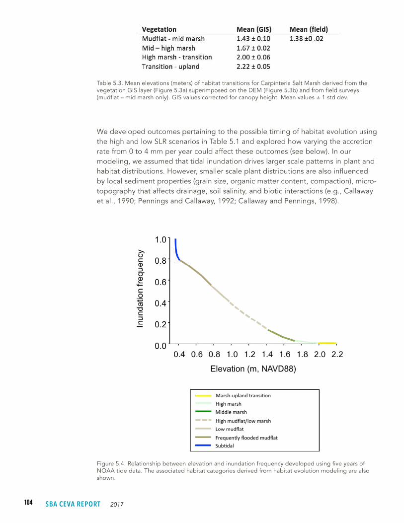
104 SBA CEVA REPORT 2017
We developed outcomes pertaining to the possible timing of habitat evolution using the high and low SLR scenarios in Table 5.1 and explored how varying the accretion rate from 0 to 4 mm per year could affect these outcomes (see below). In our modeling, we assumed that tidal inundation drives larger scale patterns in plant and habitat distributions. However, smaller scale plant distributions are also influenced by local sediment properties (grain size, organic matter content, compaction), micro-topography that affects drainage, soil salinity, and biotic interactions (e.g., Callaway et al., 1990; Pennings and Callaway, 1992; Callaway and Pennings, 1998).
Table 5.3. Mean elevations (meters) of habitat transitions for Carpinteria Salt Marsh derived from the vegetation GIS layer (Figure 5.3a) superimposed on the DEM (Figure 5.3b) and from field surveys (mudflat – mid marsh only). GIS values corrected for canopy height. Mean values ± 1 std dev.
Figure 5.4. Relationship between elevation and inundation frequency developed using five years of NOAA tide data. The associated habitat categories derived from habitat evolution modeling are also shown.

105ESTUARIES
We examined recent habitat evolution by estimating the conversion of mudflat to vegetated marsh over the past 33 years in the western portion of Carpinteria Salt Marsh (Figure 5.5) using the area measurement tool in Adobe Acrobat Pro to outline mudflat habitat in a series of aerial images taken by Pacific Western Aerial Surveys (Goleta, California) between 1980 and 2013.
Figure 5.5. Examples of encroachment of Sarcocornia into mudflat habitat adjacent to tidal creeks (1, 2) and in a small mudflat (3) over time.
106 SBA CEVA REPORT 2017
R A T E S O F M A R S H A C C R E T I O N A N D S U B S I D E N C E
Sediments eroded from the watersheds of Franklin and Santa Monica Creeks and the coastal plain during storm events are potentially deposited in Carpinteria Salt Marsh. In addition, “litterfall” and roots from marsh vegetation can contribute to accretion of the marsh surface. The balance between marsh accretion, local subsidence and SLR will influence the timing of habitat evolution. Reynolds et al. (submitted) estimated accretion rates of 3.4 to 4.5 mm per year in the top 30 cm of sediment using 210Pb. Reynolds (personal communication) suggested that an average sedimentation rate of 4 mm per year over the long term might be representative. Therefore, we explored how an average accretion rate of 4 mm per year would influence the timing of evolution of marsh habitats. Given the uncertainty in this estimate and the effect of any future changes in subsidence rates, this value provides only an example of how changes in the elevation of the marsh surface relative to the rise in sea level might affect the timing of habitat evolution. Although accretion rates may vary with location in the marsh (Reynolds, personal communication), we made the simplifying assumption that accretion rates were similar across all habitats.
E F F E C T S O F A S H O R T - T E R M S L A N O M A L Y O N M A R S H V E G E T A T I O N
During 2014–2015, a large mass of warm water off the Pacific coast of North America (the “blob”) and the El Niño of 2015 produced unusually warm sea surface temperatures and higher coastal water levels along the U.S. West Coast. In the Santa Barbara area, measurements at the NOAA tide gauge on Stearns Wharf indicated a rising sea level in 2015, with an abrupt increase to mean peak monthly anomalies of +15 to 16 cm (~6 in) above long-term MSL in September and October, followed by a decline in water levels that approached long-term MSL in early 2016 (Figure 5.6). This short-term rise in sea level provided an opportunity to explore the effects that an increase in inundation frequency could have on marsh vegetation and habitats in the future. We compared inundation frequency computed using the NOAA tidal data from September–December 2015 with water level data collected with a YSI model 600XLM V2 multiparameter water quality sonde deployed in the large tidal channel draining the western basin of Carpinteria Salt Marsh during this period. Water level data were recorded by the sonde every 15 minutes.
In October 2015, we measured marsh elevation using RTK at 1-m intervals along transects crossing mudflat and salt marsh habitat recording the condition of vegetation at each measurement point. Vegetation within a 1-m2 area surrounding each measurement was qualitatively classified as dead or dying (all brown), stressed (a mix of green and brown), or healthy (green). We then compared the observed changes in vegetation condition associated with the short-term sea level anomaly to the habitat conversion predicted to occur with longer-term sea level rise. We also took photographs in October 2015 to document the effects of increased inundation on marsh vegetation.
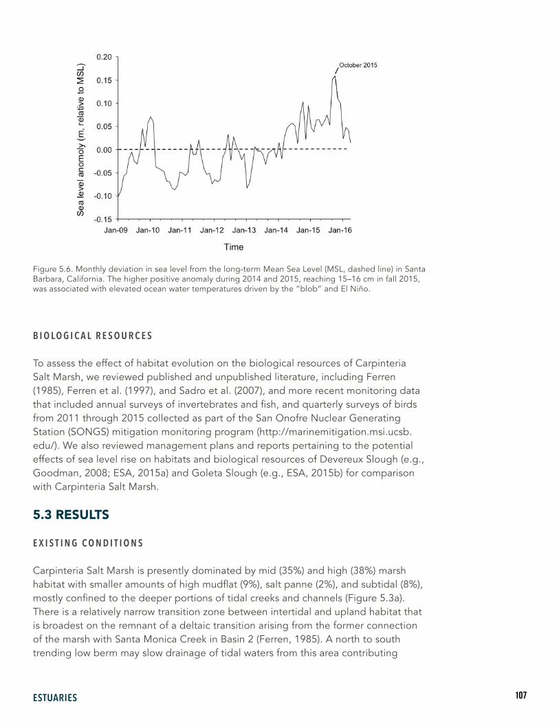
107ESTUARIES
B I O L O G I C A L R E S O U R C E S
To assess the effect of habitat evolution on the biological resources of Carpinteria Salt Marsh, we reviewed published and unpublished literature, including Ferren (1985), Ferren et al. (1997), and Sadro et al. (2007), and more recent monitoring data that included annual surveys of invertebrates and fish, and quarterly surveys of birds from 2011 through 2015 collected as part of the San Onofre Nuclear Generating Station (SONGS) mitigation monitoring program (http://marinemitigation.msi.ucsb.edu/). We also reviewed management plans and reports pertaining to the potential effects of sea level rise on habitats and biological resources of Devereux Slough (e.g., Goodman, 2008; ESA, 2015a) and Goleta Slough (e.g., ESA, 2015b) for comparison with Carpinteria Salt Marsh.
5.3 RESULTS
E X I S T I N G C O N D I T I O N S
Carpinteria Salt Marsh is presently dominated by mid (35%) and high (38%) marsh habitat with smaller amounts of high mudflat (9%), salt panne (2%), and subtidal (8%), mostly confined to the deeper portions of tidal creeks and channels (Figure 5.3a). There is a relatively narrow transition zone between intertidal and upland habitat that is broadest on the remnant of a deltaic transition arising from the former connection of the marsh with Santa Monica Creek in Basin 2 (Ferren, 1985). A north to south trending low berm may slow drainage of tidal waters from this area contributing
Figure 5.6. Monthly deviation in sea level from the long-term Mean Sea Level (MSL, dashed line) in Santa Barbara, California. The higher positive anomaly during 2014 and 2015, reaching 15–16 cm in fall 2015, was associated with elevated ocean water temperatures driven by the “blob” and El Niño.
108 SBA CEVA REPORT 2017
to the formation of a salt panne at elevations that are categorized as high marsh elsewhere in the wetland. A small amount of upland (8%) also occurs bordering the intertidal portions of the wetland, but is restricted in landward extent by surrounding residential and urban development.
T R A J E C T O R Y O F R E C E N T H A B I T A T C O N V E R S I O N
Approximately 24,000 m2 of mudflat in the western portion of the marsh (Basin 3) evolved into mid marsh from 1980 to 2013. This includes the filling in by Sarcocornia of small mudflats within viewing distance of the access road that bisects the marsh, and of the large mudflat in the western portion of Basin 3 (Figure 5.5a-c). The area of mudflat decreased continuously from 1980 to 2000, but remained relatively constant from 2007 to 2013, a period of low rainfall (Figure 5.7). It seems likely that habitat conversion was due to accretion of the marsh surface during this 33-year period, with the greatest deposition of sediment occurring during periods of heavy rainfall and along the edges of channels.
H A B I T A T E V O L U T I O N W I T H S L R
Our results suggest that the high marsh and high marsh–upland transition are initially the most vulnerable to SRL, with the conversion of these habitats to mid marsh as SLR reaches >~25 cm, relative to the marsh surface (Figures 5.8-5.9). Initially, the area of vegetated middle marsh is expected to increase as higher elevations become inundated more frequently and mixed high marsh vegetation converts to a greater cover of Sarcocornia. With a rise of sea level >25 cm, however, mid marsh may evolve more abruptly into high mudflat. This habitat is anticipated to initially increase as greater inundation of the vegetated marsh affects Sarcocornia growth and survival at lower elevations. With rising water levels, the area of mudflat is expected to further increase at the expense of vegetated marsh with high mudflat beginning to convert to low mudflat with a rise in sea level of ~60 cm relative to the marsh surface (Figures 5.8-5.9).
A caveat to the sequence of habitat evolution proposed above is the possible conversion of high mudflat to vegetated low marsh if it becomes colonized by cordgrass, Spartina foliosa. Currently, approximately one-half (6 of 13%) of the high mudflat experiences an inundation regime that supports Spartina in other wetlands. The area of potential low marsh would increase to ~30% with a SLR of up to ~36 cm, but decline with rising water levels thereafter (Figure 5.8).
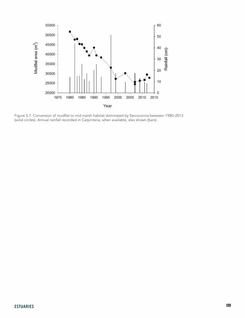
109ESTUARIES
Figure 5.7. Conversion of mudflat to mid marsh habitat dominated by Sarcocornia between 1980–2013 (solid circles). Annual rainfall recorded in Carpinteria, when available, also shown (bars).

110 SBA CEVA REPORT 2017
Figure 5.8. Habitat evolution with sea level rise scenarios assuming a) no colonization of mudflat by cordgrass Spartina foliosa, and b) colonization of portions of high mudflat by cordgrass. Also shown below these figures are the corresponding ranges of SLR predicted by the NRC (2012) for 2030, 2050, and 2100 and how an accretion rate of 4 mm per year could affect the rate of habitat evolution (*).

111ESTUARIES
Figure 5.9. Projected habitat evolution for selected scenarios of sea level rise relative to the marsh surface. A shift to a mudflat-dominated system is expected to occur with a rise in sea level of >30 cm (c). Much of the mudflat habitat created with a rise in sea level of 36 cm will have inundation frequencies that support low marsh cordgrass habitat in other tidal wetlands (d).
112 SBA CEVA REPORT 2017
There is a high level of uncertainty regarding the actual timing of habitat evolution that can be attributed to the interaction between future rates of SLR and marsh accretion. This interaction is illustrated in Table 5.4 and Figure 5.8. An accretion rate of 4 mm per year keeps pace with SLR over the next 35 years under the minimum SLR scenario, and little increase in mudflat area from existing conditions is expected (9%). Without accretion, some increase in the area of mudflat is expected (from 9% to 14%) at the expense of vegetated marsh and upland habitat. However, an accretion rate up to 4 mm per year only slows habitat conversion under the maximum SLR scenario. In this case, mudflat habitat would increase from 9% to 56% with accretion (compared with 70% without accretion). Over the longer term, the minimum and maximum SLR scenarios diverge such that accretion rates of up to 4 mm per year do not appreciably alter the evolution of vegetated marsh to mudflat under the maximum SLR scenario. In this case, the wetland could consist of >80% mudflat by the end of the 21st century with or without accretion, and likely remain a mudflat-dominated system for many years (Figure 5.8). In contrast, under the minimum SLR scenario, little change in area of mudflat is expected by the end of the century if the marsh surface accretes at 4 mm per year.
T I D A L D Y N A M I C S A N D T H E S H O R T - T E R M S E A L E V E L A N O M A L Y
We compared the elevation-inundation frequency relationship derived from the five years of NOAA tide data used in modeling to data from NOAA and in situ monitoring for the months of July-August, September-October, and November-December 2015. These months covered the period of highest positive sea level anomaly. Inundation frequencies computed for an elevation of 1.4 m NAVD88 (approximately Mean High Water [MHW], Tables 5.5, 5.6a) using the NOAA data for July–December 2015 are elevated relative to the five-year average (0.14), with peak inundation (0.28) occurring September-October (Table 5.6a). This increase in inundation would be sufficient to shift habitat from pickleweed dominated mid marsh to high mudflat, based on the relationship between inundation, elevation and habitat (Table 5.6a, Figure 5.10). The in situ datalogger measurements indicated that the NOAA data underestimated the actual inundation in the marsh at this elevation by ~20% (Table 5.6a). During the peak anomaly in September-October, inundation frequency expected for an elevation of 1.4 m, the approximate lower boundary of pickleweed, was equivalent to that of elevations of 1.15 m and 1.04 m from the NOAA and CSM datasets, respectively, and typical of mudflat habitat.
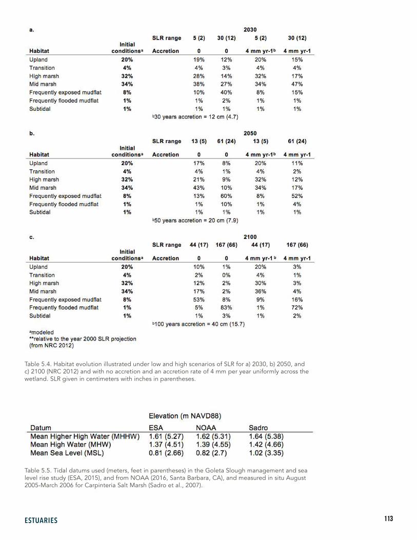
113ESTUARIES
Table 5.4. Habitat evolution illustrated under low and high scenarios of SLR for a) 2030, b) 2050, and c) 2100 (NRC 2012) and with no accretion and an accretion rate of 4 mm per year uniformly across the wetland. SLR given in centimeters with inches in parentheses.
Table 5.5. Tidal datums used (meters, feet in parentheses) in the Goleta Slough management and sea level rise study (ESA, 2015), and from NOAA (2016, Santa Barbara, CA), and measured in situ August 2005-March 2006 for Carpinteria Salt Marsh (Sadro et al., 2007).
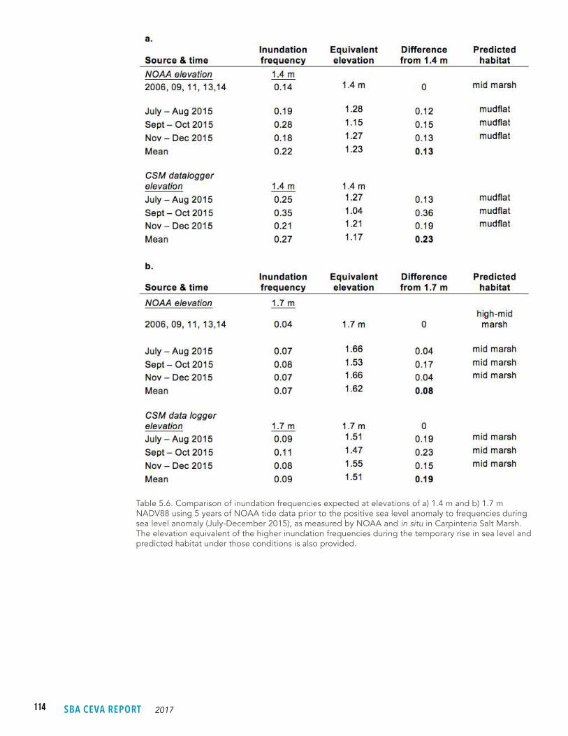
114 SBA CEVA REPORT 2017
Table 5.6. Comparison of inundation frequencies expected at elevations of a) 1.4 m and b) 1.7 m NADV88 using 5 years of NOAA tide data prior to the positive sea level anomaly to frequencies during sea level anomaly (July-December 2015), as measured by NOAA and in situ in Carpinteria Salt Marsh. The elevation equivalent of the higher inundation frequencies during the temporary rise in sea level and predicted habitat under those conditions is also provided.
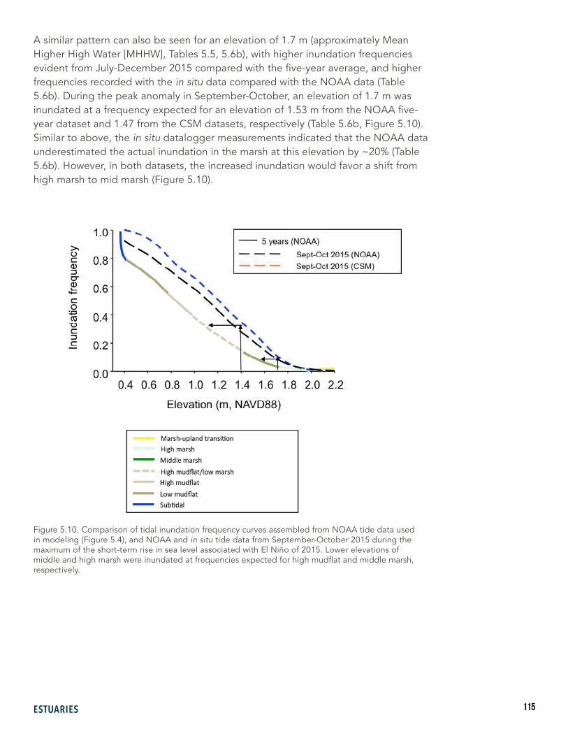
115ESTUARIES
A similar pattern can also be seen for an elevation of 1.7 m (approximately Mean Higher High Water [MHHW], Tables 5.5, 5.6b), with higher inundation frequencies evident from July-December 2015 compared with the five-year average, and higher frequencies recorded with the in situ data compared with the NOAA data (Table 5.6b). During the peak anomaly in September-October, an elevation of 1.7 m was inundated at a frequency expected for an elevation of 1.53 m from the NOAA five-year dataset and 1.47 from the CSM datasets, respectively (Table 5.6b, Figure 5.10). Similar to above, the in situ datalogger measurements indicated that the NOAA data underestimated the actual inundation in the marsh at this elevation by ~20% (Table 5.6b). However, in both datasets, the increased inundation would favor a shift from high marsh to mid marsh (Figure 5.10).
Figure 5.10. Comparison of tidal inundation frequency curves assembled from NOAA tide data used in modeling (Figure 5.4), and NOAA and in situ tide data from September-October 2015 during the maximum of the short-term rise in sea level associated with El Niño of 2015. Lower elevations of middle and high marsh were inundated at frequencies expected for high mudflat and middle marsh, respectively.
116 SBA CEVA REPORT 2017
M O D E L C O N G R U E N C E W I T H T H E S H O R T - T E R M S L R A N O M A L Y
Observations in the marsh were consistent with predictions of the inundation-elevation-habitat relationships used in the habitat evolution model. Marsh vegetation at lower tidal elevations was stressed by the elevated sea levels of fall 2015 (Table 5.6, Figure 5.11). Areas of Sarcocornia that appeared stressed or dying (all brown) occurred at an average elevation of ~1.48 m (4.86’) NAVD88, higher than the average mudflat–mid marsh transitions of ~1.4 m (Tables 4.3, 4.7). Sarcocornia between ~1.48 m and 1.52 m (4.98’) was largely brown with some green and appeared to be stressed. Sarcocornia higher than ~1.68 m (5.51’) appeared healthy as evident by green stems. The shift upward in elevation of ~25-30 cm between the lowest elevational occurrence of healthy Sarcocornia prior to the sea level anomaly (Table 5.3) and the lowest occurrence of healthy Sarcocornia in fall 2015 (Table 5.7) anticipates a shift in habitat from mid marsh to mudflat based on the elevation-inundation frequency relationships used in modeling and recorded in the marsh during the short term SL anomaly (Table 5.6, Figure 5.10).
B I O L O G I C A L R E S O U R C E S O F P A R T I C U L A R I N T E R E S T
Fourteen of 16 plant species of conservation concern reported from Carpinteria Salt Marsh are found in the high marsh and transition habitat and initially the most vulnerable to SLR (Table 5.8). Of particular interest is the federally listed endangered salt marsh bird’s-beak, restricted to higher elevations with sandier soils, and Coulter’s goldfields, a species of Federal Management Concern, also found in areas with sandier soils and alluvial deposits (Ferren, 1985). In addition, the federal and California listed endangered Ventura marsh milkvetch has been planted in the wetland as part of a recovery plan for the species and is vulnerable to increased inundation with SLR.

117ESTUARIES
Figure 5.11. Photographs taken on October 23, 2015 showing band of brown Sarcocornia (Salicornia) adjacent to a tidal creek and at lower elevations in the background indicative of greater inundation associated with elevated sea levels during the El Niño.
a.
b.
Table 5.7. Mean elevations (meters) of bare (mudflat), brown (stressed) vegetation, and green (healthy) vegetation derived from field surveys conducted in October 2015. Mean values ±1 std dev; n = 10 transects.

118 SBA CEVA REPORT 2017
Table 5.8. List of selected plant species of special interest reported from Carpinteria Salt Marsh (CSM), Goleta Slough, and Devereux Slough, typical habitat occupied, and conservation status. Fourteen of 16 species are found in high marsh/transition habitat.
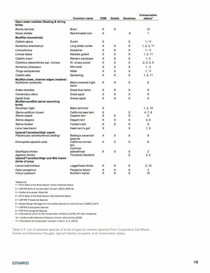
119ESTUARIES
Table 5.9. List of selected species of birds of special interest reported from Carpinteria Salt Marsh, Goleta and Devereux Sloughs, typical habitat occupied, and conservation status.
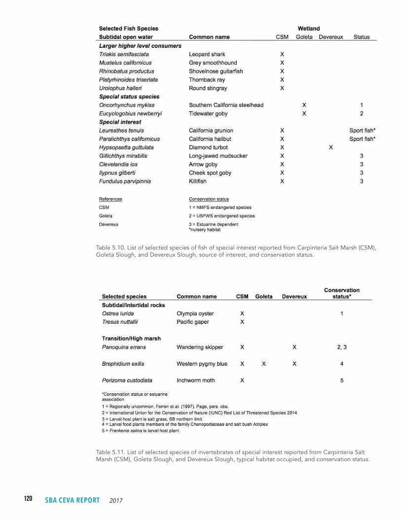
120 SBA CEVA REPORT 2017
Table 5.10. List of selected species of fish of special interest reported from Carpinteria Salt Marsh (CSM), Goleta Slough, and Devereux Slough, source of interest, and conservation status.
Table 5.11. List of selected species of invertebrates of special interest reported from Carpinteria Salt Marsh (CSM), Goleta Slough, and Devereux Slough, typical habitat occupied, and conservation status.
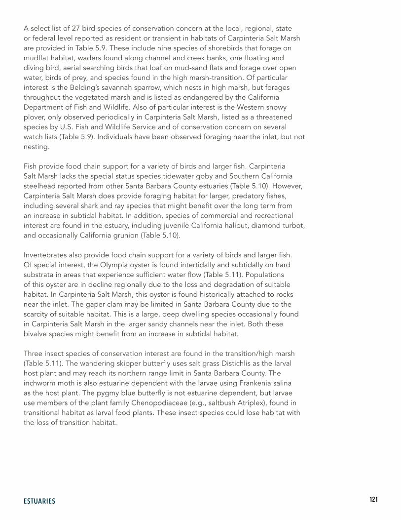
121ESTUARIES
A select list of 27 bird species of conservation concern at the local, regional, state or federal level reported as resident or transient in habitats of Carpinteria Salt Marsh are provided in Table 5.9. These include nine species of shorebirds that forage on mudflat habitat, waders found along channel and creek banks, one floating and diving bird, aerial searching birds that loaf on mud-sand flats and forage over open water, birds of prey, and species found in the high marsh-transition. Of particular interest is the Belding’s savannah sparrow, which nests in high marsh, but forages throughout the vegetated marsh and is listed as endangered by the California Department of Fish and Wildlife. Also of particular interest is the Western snowy plover, only observed periodically in Carpinteria Salt Marsh, listed as a threatened species by U.S. Fish and Wildlife Service and of conservation concern on several watch lists (Table 5.9). Individuals have been observed foraging near the inlet, but not nesting.
Fish provide food chain support for a variety of birds and larger fish. Carpinteria Salt Marsh lacks the special status species tidewater goby and Southern California steelhead reported from other Santa Barbara County estuaries (Table 5.10). However, Carpinteria Salt Marsh does provide foraging habitat for larger, predatory fishes, including several shark and ray species that might benefit over the long term from an increase in subtidal habitat. In addition, species of commercial and recreational interest are found in the estuary, including juvenile California halibut, diamond turbot, and occasionally California grunion (Table 5.10).
Invertebrates also provide food chain support for a variety of birds and larger fish. Of special interest, the Olympia oyster is found intertidally and subtidally on hard substrata in areas that experience sufficient water flow (Table 5.11). Populations of this oyster are in decline regionally due to the loss and degradation of suitable habitat. In Carpinteria Salt Marsh, this oyster is found historically attached to rocks near the inlet. The gaper clam may be limited in Santa Barbara County due to the scarcity of suitable habitat. This is a large, deep dwelling species occasionally found in Carpinteria Salt Marsh in the larger sandy channels near the inlet. Both these bivalve species might benefit from an increase in subtidal habitat.
Three insect species of conservation interest are found in the transition/high marsh (Table 5.11). The wandering skipper butterfly uses salt grass Distichlis as the larval host plant and may reach its northern range limit in Santa Barbara County. The inchworm moth is also estuarine dependent with the larvae using Frankenia salina as the host plant. The pygmy blue butterfly is not estuarine dependent, but larvae use members of the plant family Chenopodiaceae (e.g., saltbush Atriplex), found in transitional habitat as larval food plants. These insect species could lose habitat with the loss of transition habitat.
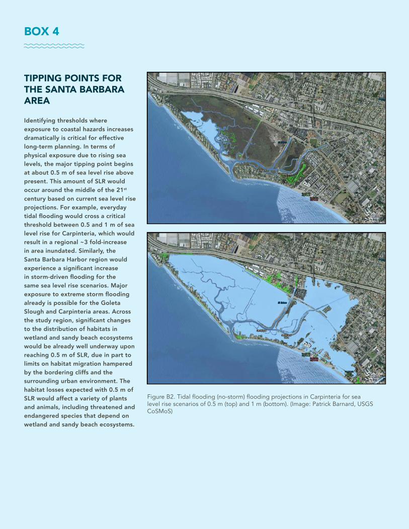
122 SBA CEVA REPORT 2017
BOX 4
TIPPING POINTS FOR THE SANTA BARBARA AREA
Identifying thresholds where exposure to coastal hazards increases dramatically is critical for effective long-term planning. In terms of physical exposure due to rising sea levels, the major tipping point begins at about 0.5 m of sea level rise above present. This amount of SLR would occur around the middle of the 21st century based on current sea level rise projections. For example, everyday tidal flooding would cross a critical threshold between 0.5 and 1 m of sea level rise for Carpinteria, which would result in a regional ~3 fold-increase in area inundated. Similarly, the Santa Barbara Harbor region would experience a significant increase in storm-driven flooding for the same sea level rise scenarios. Major exposure to extreme storm flooding already is possible for the Goleta Slough and Carpinteria areas. Across the study region, significant changes to the distribution of habitats in wetland and sandy beach ecosystems would be already well underway upon reaching 0.5 m of SLR, due in part to limits on habitat migration hampered by the bordering cliffs and the surrounding urban environment. The habitat losses expected with 0.5 m of SLR would affect a variety of plants and animals, including threatened and endangered species that depend on wetland and sandy beach ecosystems.
Figure B2. Tidal flooding (no-storm) flooding projections in Carpinteria for sea level rise scenarios of 0.5 m (top) and 1 m (bottom). (Image: Patrick Barnard, USGS CoSMoS)
123ESTUARIES
O V E R V I E W C O M P A R I S O N O F C A R P I N T E R I A S A L T M A R S H W I T H D E V E R E U X A N D G O L E T A S L O U G H S
Devereux Slough in contrast to Carpinteria Salt Marsh is generally closed to tidal exchange by a sand berm at the inlet (Collins and Melack, 2014). The inlet occasionally opens to the ocean after large rainfall events when freshwater runoff trapped behind the berm rises to the height of the berm, leading to overtopping, erosion and formation of an inlet channel (ESA 2015a). The duration of tidal exchange is typically short (<20 days), with sand re-deposited in the inlet over time leading to eventual closure.
Devereux Slough contains an assemblage of salt marsh plant species similar to, though less diverse, than that found in Carpinteria Salt Marsh with the lower elevations dominated by Sarcocornia pacifica and higher elevations characterized by a mixed assemblage that includes S. pacifica, Frankenia salina, D. spicata, and Arthrocnemum subterminale (Table 5.8). The ponding created by the berm at the inlet has contributed to a shift upward in the elevation of mudflats and of marsh vegetation relative to fully tidal wetlands (Figure 5.12). Much of what is currently mud/salt flat during the summer-fall months and ponded open water during the winter months is at an elevation equivalent to high marsh habitat at Carpinteria Salt Marsh (Figure 5.13).
Figure 5.12. Comparison of elevational distribution of habitats in Devereux Slough with Carpinteria Salt Marsh.

124 SBA CEVA REPORT 2017
a.
b.
Figure 5.13. Expected distribution of interidal habitats in Devereux Slough if the wetland were fully tidal. Much of the current mud/salt flat (red arrow) occurs at elevations occupied by high (mixed) marsh vegetation at Carpinteria Salt Marsh.
125ESTUARIES
In contrast to Devereux Slough, Goleta Slough had been a fully tidal wetland with the inlet maintained open through the removal of sand accumulation by the Santa Barbara County Flood Control District (SBCFCD) since the mid-1990s (ESA 2015b). However, beginning in 2013, the inlet has been allowed to close due to the accumulation of sand and the formation of a berm at the beach that restricts or prevents tidal exchange. Inlet closure lasts until the berm is breached, an event naturally associated with a storm runoff event that overtops the berm and scours a channel reintroducing tidal exchange to the slough, or through a manual opening conducted to protect the Santa Barbara Airport and surrounding infrastructure from flooding. In the absence of significant freshwater inputs, water levels in Goleta Slough are controlled by the tides and structures inside the wetland that restrict flow (tide gates, levees) when the inlet is open, and by the elevation of the beach berm when the inlet is closed (ESA, 2015b).
The biological communities of Goleta Slough closely resemble those of Carpinteria Salt Marsh and include a number of plant and animal species that reach their northern distributional limits in this wetland (Zedler, 1982) (Tables 5.8-11). Potential effects of SLR on these habitats, assuming full tidal exchange, were analyzed in ESA (2015b) and are only briefly reviewed here. In their study of Goleta Slough, ESA (2015b) used the Sea Level Affecting Marshes Model (SLAMM), and a simple conceptual habitat evolution model based on inundation frequency similar to that also used by us for Carpinteria Salt Marsh, to evaluate potential changes in habitat distributions assuming a fully tidal wetland with possible SLR scenarios for 2050 and 2100. Elevations associated with six representative habitat categories were applied to coastal LiDAR topography to map existing habitats and changes in habitats across the wetland with SLR. Projections were based on the expected amount of future sea level rise and two accretion rate (3 mm or 5 mm per year) scenarios.
Although there were some differences in model outcomes, both the SLAMM and inundation frequency models predicted the extensive conversion of vegetated marsh habitat to mudflat under the two accretion rate scenarios by the end of the century under fully tidal conditions. They did not consider the possible colonization of cordgrass or eelgrass. Habitat evolution modeling furthermore predicted the transgression of transitional and high marsh habitat into upland under future SLR conditions. ESA (2015b) noted that transitional habitat may migrate upslope and across tidal barriers such as berms and levees, displacing existing upland habitat. Similar to Carpinteria Salt Marsh, the availability of convertible upland habitats is limited by existing infrastructure, including the Santa Barbara Airport.
However, even though final regulatory decisions are not settled, under the current management, the inlet mouth is not kept open and water levels in Goleta Slough are controlled primarily by freshwater inputs and the height of the sand berm at the inlet, which blocks tidal exchange. ESA (2015b) further modeled the consequences of an intermittently open inlet on slough water levels and inlet closure frequency in the face of expected SLR. Initially, it is anticipated that Goleta Slough will develop the characteristics of an intermittently open tidal wetland, remaining closed for much of
126 SBA CEVA REPORT 2017
the year in the absence of significant storm runoff, similar to Devereux Slough. ESA (2015b) hypothesized that an intermittently open inlet for Goleta Slough would result in the ponding of runoff behind the beach berm. Habitat conversion would occur as higher elevation wetland converts to uplands in the absence of tidal inundation during high tides, and mid and higher marsh vegetation would shift upward in elevation as the lower elevations spend more time submerged in a pattern similar to that of Devereux Slough. Much of the vegetated marsh at lower elevations would convert to seasonally inundated mudflats that would be submerged during the rainy season due to the trapping of freshwater runoff behind the beach berm, but dry by late spring or summer.
The effect of SLR on the habitats of both Devereux and Goleta Sloughs depends on how rising ocean water levels (and any long-term changes in fluvial inputs) influence inlet dynamics: the height of the berm at the beach and frequency of inlet opening, and thus tidal exchange. For both Devereux and Goleta Sloughs, ESA anticipates that the beach berm will increase in height, initially keeping pace with SLR. The increase in berm height will trap a greater volume of freshwater runoff, creating a larger ponded area landward of the berm over time. For example, the modeling suggested that the volume of Devereux Slough will double to quadruple the existing volume with a SLR of ~91 cm (3’). This could lead to a further shift in habitats upward in elevation as vegetation at lower elevations becomes submerged more frequently and dies, while the higher water levels will allow for the transgression of marsh vegetation upward into transition, upland and riparian habitat. At some point in time, modeling by ESA suggests that SLR will increase the length of time that the inlets of Devereux and Goleta Sloughs remain open following a breaching event due to the larger tidal prism or volume of water exchanged when the inlet is open. However, since a larger volume of water, and thus more runoff, will be required to breach the inlets, they may also be closed more frequently than at present during dry years. Because Devereux is smaller than Goleta Slough, with a smaller potential tidal prism, that wetland may remain closed more often into the future than Goleta. For Goleta Slough, because of a larger potential tidal prism, modeling suggests that this wetland could approach fully tidal conditions with a SLR of >~0.91 m (3’). Interestingly, in Goleta Slough, vegetated marsh in both an intermittently open and a fully tidal system may evolve with SLR into mudflat, initially more similar to that present at Devereux, then with greater tidal exchange more similar to that at Carpinteria Salt Marsh.
Similar to Carpinteria Salt Marsh, the rate of accretion of the marsh surface, along with SLR will affect the rate of habitat evolution in both Devereux and Goleta Sloughs. For example, ESA estimated that with the loss of tidal prism associated with 0.6 m (2’) of accretion in Devereux Slough, the effect of 0.9 m (3’) of SLR on the frequency of inlet opening is diminished, and the slough could remain primarily closed, similar to existing conditions. The effect of a planned restoration in Devereux Slough, including the removal of 300,000 cubic yards of fill to enlarge upper Devereux, on the frequency of inlet opening remains under study.

127ESTUARIES
5.4 DISCUSSION
The estuarine wetlands of Santa Barbara County are extremely vulnerable to the effects of sea level rise. In small, fully tidal systems, such as Carpinteria Salt Marsh, rising sea level will increase tidal inundation of the marsh surface leading to changes in key physical and biological properties known to structure marsh plant communities and habitats (reviewed in Grewell et al., 2007). The frequency of tidal inundation affects soil moisture and salinity, and oxygen content (Mahall and Park, 1976a-c; Watson and Byrne, 2009), and modulates species interactions such that inter-specific competition that can define plant community boundaries (Pennings and Callaway, 1992; Pennings et al., 2005). Tidal inundation frequency is closely linked to marsh surface elevation, and the distribution of marsh plants typically varies along an elevational gradient (Zedler, 1982; Zedler et al., 1999). As a result, habitat “zones” defined by characteristic vegetation can be observed extending from low to high elevations in most Southern California estuaries, including Carpinteria Salt Marsh (Ferren, 1985; Page et al. ,2003; Sadro et al., 2007). However, marsh elevation per se is only an approximate proxy for inundation environment because differences in local hydrology influenced by inlet dynamics, wetland topography, and soil characteristics can affect the relationship between these variables, and the specific mix of vegetation within these zones can differ among estuaries (Zedler, 1982; Thorne et al., 2016). To explore potential changes in estuarine ecosystems with SLR it is most insightful to examine the relationship between inundation frequency, elevation, and vegetation for each wetland of interest.
At Carpinteria Salt Marsh, and likely other tidal wetlands in the region, the tidal datums of mean high water (MHW) and mean higher high water (MHHW) appear to be approximate “critical tide” levels (sensu Doty, 1946), important in defining vegetation community transitions. At elevations higher than approximately MHHW, plant species richness in Carpinteria Salt Marsh increases from a near monoculture of Sarcocornia below this datum to a mix of Sarcocornia and other species that include regionally rare and endangered species above this datum. At elevations below MHW, Sarcocornia is more likely to be sparse with a transition to mudflat in Carpinteria Salt Marsh. SLR will cause a shift upward in these tidal datums and in plant distributions.
The dying and stressed vegetation associated with the positive sea level anomaly of 2015 further illustrates the important role that inundation environment has in structuring marsh plant communities and habitats. The increase in Mean Sea Level of ~36 cm observed in September-October 2015 inside Carpinteria Salt Marsh was comparable to the high SLR scenario for 2030 and mid-range SLR scenario for 2050 of approximately ~30 cm (Figure 5.2). The response of vegetation to the increase in inundation associated with this short-term phenomenon was congruent with our predictions of extensive habitat conversion of vegetated salt marsh to mudflat with this amount of SLR.
128 SBA CEVA REPORT 2017
The importance of inundation regime to habitat distributions is illustrated in Devereux Slough. In this wetland, rarely open to tidal exchange, the general zonation of habitats is similar to Carpinteria Salt Marsh, with Sarcocornia dominant lower and a mix of species higher, but the zones are shifted higher in elevation. The presence of a sand berm at the inlet of this estuary that blocks tidal exchange most of the year allows for the trapping of storm runoff and the seasonal formation of an open water lagoon at elevations occupied by high marsh habitat at Carpinteria Salt Marsh. During the summer and fall months, the lagoon dries up in the absence of significant freshwater inputs, leaving mud/salt flats. The elevational boundaries of vegetation in Devereux Slough are presumably shifted higher due to physiological stresses associated with sustained inundation of lower elevations in the winter months, and perhaps salinity stress during sustained exposure during drier months of the year.
Although little net change in the overall area of vegetated marsh is predicted up to about 20 cm of SLR, our modeling exercise revealed that the high salt marsh and transition habitats are the most immediately vulnerable to rising water levels, continuously declining in area and evolving into mid marsh habitat unless there are opportunities for these habitats to transgress into upland. If these high salt marsh and transitional habitats are lost, it is expected that there will be a loss of plant biodiversity, including regionally rare, threatened and endangered plants, such as the salt marsh bird’s-beak, a loss of foraging and nesting habitat for the endangered Belding’s savannah sparrow, and nursery habitat for marsh insects (Appendix 5.1). The mid marsh is initially less vulnerable and will increase in area, but eventually convert to mudflat with the loss of habitat for Belding’s savannah sparrow, as well as algal and detrital production and habitat used by marsh invertebrates (Appendix 5.2). The consequences for carbon sequestration will be significant if lower intertidal zones convert to mudflat with no colonization by cordgrass or eelgrass.
Our study also indicates a threshold of ~30 cm when an abrupt increase in the proportion of mudflat habitat is expected as vegetated marsh is inundated more frequently. The mudflat and subtidal habitats, which are expected to increase in area over time, are the least vulnerable to the adverse impacts of SLR. The increase in area of mudflat could benefit shorebirds that use this habitat for foraging and loafing, and wading and water birds may also benefit with increase in the amount of open water habitat (Appendix 5.3). Some fish (e.g., halibut) could benefit from the increase in foraging area or nursery habitat (Appendix 5.4).
Because of the beach berm blocking tidal exchange, intermittently open estuaries such as Devereux and Goleta Slough would initially appear to be less vulnerable to SLR than Carpinteria Salt Marsh. However, our review of the modeling scenarios conducted by ESA (2015a, b) indicates that SLR may indirectly facilitate a shift in vegetation and habitat distributions upslope due to the expected higher berm height and volume of storm runoff trapped behind the berm. In both fully tidal and intermittently open estuaries, there will be a loss of sensitive biological resources if the displaced habitats are unable to transgress into upland habitat. Our general findings that anticipate an increase in mudflat habitat by the end of the century if
129ESTUARIES
SLR exceeds accretion rate are congruent with those of ESA (2015b) for a fully tidal Goleta Slough, and with a recently completed study of several California wetlands, including portions of Mugu Lagoon, the largest fully tidal estuary in closest proximity to Carpinteria Salt Marsh (Thorne et al., 2016).
We used a simple habitat evolution model based on existing conditions to estimate changes in the distribution and area of marsh habitat with SLR. Predictions of extensive conversion of vegetated marsh to mudflat with a SLR of ~25 cm were generally supported by measurements and observations of the poor condition of vegetation inundated more frequently by the higher tides associated with the El Niño of 2015. However, our habitat evolution model assumes that the relationship between inundation and elevation, based on existing conditions, will hold in the future, but there is some evidence that it may not and that we may underestimate the rate of habitat evolution using the NOAA data.
There is the suggestion in the comparison of NOAA data to data collected in situ during the peak El Niño sea level anomaly that the difference between water levels measured for the open coast and those inside the marsh may increase with SLR, at least initially. The tide cycle in Carpinteria Salt Marsh, and other coastal wetlands, is typically not symmetrical (Hubbard, 1996). Ebbing tides take longer to drain from the marsh than flood tides take to fill it. One possible mechanism to explain the higher tides in the marsh as coastal water levels rose, is that the marsh has increasingly less time to drain during ebb tides before the following flood tide pushes water back inside, raising water levels above those predicted for the coastal ocean. This phenomenon would contribute to an underestimation of inundation frequency at higher elevations, and consequently in the rate of habitat evolution if based solely on coastal tide data.
Accretion of the marsh surface will counteract the effects of SLR, slowing the rate of habitat evolution, but we have no information on how accretion rates may change in the future. Large volumes of sediments currently enter the marsh in storm runoff, despite the debris basins on upper Santa Monica and Franklin Creeks and a siltation basin on Via Real, just north of the marsh that traps sediment. Some of these sediments are deposited in the marsh during storms, and the extensive conversion of mudflat to mid marsh over the past 33 years supports the view that current accretion rates exceeded SLR over that period. Currently, the impact of sedimentation on the marsh ecosystem is a priority management concern because of the importance of mudflat as feeding and loafing habitat for shorebirds (Ferren et al., 1997). Over the short term, an increase in the rate of SLR may stabilize existing habitats, offsetting sediment accretion. Over the longer term, if accretion is unable to keep pace with rising water levels, the conversion of mid marsh to mudflat is likely to occur.
Additional uncertainty in forecasting the effects of SLR on marsh habitats relates to possible changes in the frequency and intensity of extreme storm events with consequences for freshwater runoff and sediment transport into coastal estuaries that could affect tidal prism, erosion rates, and frequency of inlet opening (Zedler, 2010;

130 SBA CEVA REPORT 2017
Barnard et al., 2017; Feng et al., unpublished ms, Sections 2, 4 this report). There is uncertainty and little consensus regarding future changes in rainfall patterns over next 100 years (PRBO, 2011, Sections 2, 4 this report). Climate model projections indicate that as climate warms, there may be a tendency for dry days to occur more often (e.g., longer dry spells), but occasional days with heavy precipitation and runoff to become more extreme (Feng et al., unpublished ms, Section 2 this report). Some of the greatest impacts to Santa Barbara County coastal wetlands will likely occur during these extreme events, for example, when the highest spring tides and ocean waves coincide with winter storm runoff during a large El Niño year, reinforced by SLR. In such cases tidal waters will reach and exceed extreme high water of approximately 2.1 m NAVD88. An increase in the frequency and magnitude of extreme events could accelerate habitat conversion, for example, of mid marsh to mudflat, and of upland to transition through effects on soil moisture and salinity. Conversely, elevated sediment transport into the marsh during these events could act to ameliorate SLR effects.
Given the uncertainty in rates of relative SLR, and in the effects of other climatic factors on the evolution of marsh habitats, time of year is not a useful trigger point to initiate adaptive management. Rather, it seems reasonable to develop trigger points, and a strategy that could be implemented once the trigger is reached. This approach applies to all three wetlands. If preservation of high marsh-transition habitat is a priority, adaptation will have to be initiated sooner rather than later, but care must be taken not to adversely affect existing wetland functioning through the addition of sediment, infrastructure or other measures. We suggest using information on the balance between rising water levels and accretion rates as one set of trigger points to initiate adaptive action.
5.5 KEY FINDINGS
• In Carpinteria Salt Marsh, vegetated marsh will convert to mudflat with rising sea level, but the timing of habitat evolution varies with SLR scenario and assumptions regarding accretion rate of the marsh surface.
• Our results suggest that the high marsh and upland transition are initially the most vulnerable to SLR, with the conversion of these habitats to mid marsh as SLR reaches >~25 cm, relative to the marsh surface. Initially, the area of vegetated middle marsh is expected to increase as higher elevations become inundated more frequently and mixed high marsh vegetation converts to a greater cover of Sarcocornia.
• With a rise of sea level >25 cm relative to the marsh surface, mid marsh may evolve more abruptly into high mudflat as greater inundation of the vegetated marsh affects Sarcocornia growth and survival at lower elevations.
• Estimates of the rates of habitat conversion of vegetated marsh to mudflat for Carpinteria Salt Marsh vary widely from little change (9% of existing habitat) (low

131ESTUARIES
emissions scenario, high accretion) to >80% of habitat (business as usual scenario, no accretion) by the end of the century.
• Fourteen of 16 plant species of conservation concern (threatened, rare or endangered) reported from Carpinteria Salt Marsh are found in the high marsh and transition habitat and initially the most vulnerable to SLR. These include the salt marsh bird’s-beak and Coulter’s goldfields. The federal and California listed endangered Ventura marsh milkvetch has been planted in the wetland as part of a recovery plan for the species and is vulnerable to increased inundation with SLR.
• Nesting habitat for California listed endangered Belding’s savannah sparrow will be lost with the conversion of vegetated marsh to mudflat.
• Over the past 33 years, approximately 50% of tidal mudflat in the western portion of Carpinteria Salt Marsh has converted to mid marsh habitat likely due to marsh accretion. A small increase in SLR over present may reduce the conversion of tidal mudflat to vegetated salt marsh.
• Devereux Slough has historically been non-tidal for most of the year with tidal exchange blocked by a sand berm at the inlet. Plant distributions are shifted higher in Devereux than Carpinteria Salt Marsh due to the formation of a lagoon during the winter that submerges lower elevations. ESA (2015a) modeling of lagoon water levels with SLR suggests that plant and habitat distributions may shift even higher in Devereux, depending on rates of accretion of the slough surface.
• The effects of SLR on Goleta Slough were first modeled by ESA (2015b) assuming open inlet conditions and generally conform to our results for Carpinteria Salt Marsh (conversion of some vegetated marsh to mudflat by 2100). Goleta Slough has recently (2013) been allowed to close and may develop habitat characteristics more similar to Devereux Slough as water ponded behind the beach berm could cause the conversion of vegetated marsh to mudflat at lower elevations and the transgression of marsh vegetation into transition, and upland habitat at higher elevations. However, modeling by ESA (2015b) suggested that eventually the greater tidal prism in Goleta Slough may allow the inlet to remain open longer following breaching events and that the wetland could become largely tidal with 3 ft (0.9 m) of SLR, and thus experience shifts upward in habitat distributions similar to Carpinteria Salt Marsh.
• For vulnerable species of wetland birds, plants and insects to persist, avenues for inland migration need to be identified. For Devereux Slough, which is mostly unhindered by development, ESA modeling suggests plant distributions will shift higher into the surrounding natural area. Inland transgression is more difficult for Carpinteria Salt Marsh and Goleta Slough, which are confined by infrastructure, buildings, and agricultural land. Creative solutions will be important.
132 SBA CEVA REPORT 2017
• The uncertainty regarding timing of SLR creates challenges for land use planners since any implemented adaptation strategy to accommodate future SLR should not adversely affect the existing functioning of the wetland (e.g., by increasing sediment delivery, introduction of infrastructure). The monitoring of indicators reflective of SLR within Santa Barbara County coastal wetlands (e.g., long-term trends in water levels, marsh accretion rates) and the development of trigger points would be useful to inform the timing of implementation of a particular adaptation strategy.
• Data gaps or areas of uncertainty that exist regarding the response to all three wetlands to SLR is how (or if) beach dynamics (sand supply and transport, erosion) will change in the future to influence the frequency of inlet opening and thus tidal exchange and whether fluvial inputs will change to appreciably affect marsh accretion rates and modify the distribution and timing of changes in habitats.

133ESTUARIES
Appendix 5.1. Potential effects of SLR on high salt marsh and transition habitats.

134 SBA CEVA REPORT 2017
Appendix 5.2. Potential effects of SLR on middle salt marsh habitat.
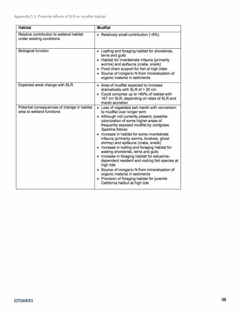
135ESTUARIES
Appendix 5.3. Potential effects of SLR on mudflat habitat.

136 SBA CEVA REPORT 2017
Appendix 5.4. Potential effects of SLR on subtidal habitat.
Dave H
ubb
ard
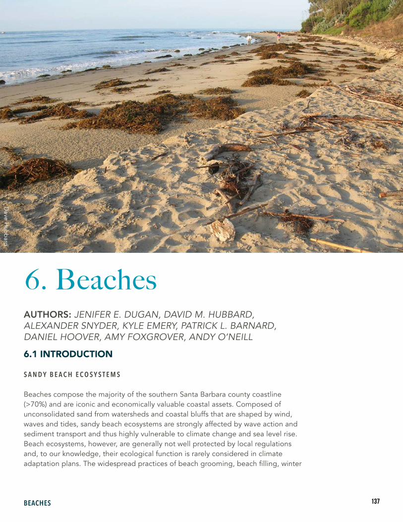
137BEACHES
6. BeachesAUTHORS: JENIFER E. DUGAN, DAVID M. HUBBARD, ALEXANDER SNYDER, KYLE EMERY, PATRICK L. BARNARD, DANIEL HOOVER, AMY FOXGROVER, ANDY O’NEILL
6.1 INTRODUCTION
S A N D Y B E A C H E C O S Y S T E M S
Beaches compose the majority of the southern Santa Barbara county coastline (>70%) and are iconic and economically valuable coastal assets. Composed of unconsolidated sand from watersheds and coastal bluffs that are shaped by wind, waves and tides, sandy beach ecosystems are strongly affected by wave action and sediment transport and thus highly vulnerable to climate change and sea level rise. Beach ecosystems, however, are generally not well protected by local regulations and, to our knowledge, their ecological function is rarely considered in climate adaptation plans. The widespread practices of beach grooming, beach filling, winter
Dave H
ubb
ard
138 SBA CEVA REPORT 2017
berm building, shoreline armoring and vehicle use that degrade beach ecosystems (Defeo et al., 2009) occur on beaches in the study region.
Although often less appreciated for ecological values than other shoreline types, sandy beaches are vitally important coastal ecosystems supporting a diverse and unique biota and key ecological functions in the study area and many regions of the world (Brown and McLachlan, 2002; Schlacher et al., 2007). Ecosystem services and functions of beaches and dunes in the study area include absorption of wave energy, the filtration of large volumes of seawater, nutrient recycling, rich endemic invertebrate communities that are important prey resources for shorebirds and fish, and the provision of critical habitat for pinnipeds, and declining and endangered wildlife, such as shorebirds, as well as beach-nesting fish (Dugan and Hubbard, 2016). Wider beaches in the study area can also support sand-trapping pioneering vegetation, including unique plants and coastal strand communities (Dugan and Hubbard, 2010).
Exposed sandy beaches have been classified by a variety of schemes based on exposure, profiles and wave climate (Brown and McLachlan, 1990). Coastal configuration and orientation to prevailing swells have strong effects on the geomorphology of beaches (Habel and Armstrong, 1978). In Santa Barbara County, coastal exposure changes significantly at Point Conception, where the orientation of the mainland coast shifts 90 degrees, running nearly east for ~60 miles. This orientation shelters the southern Santa Barbara County coastline from the dominant northwest swells that affect the north County coast. The result is that storm waves south of Point Conception are approximately half the height of those north of the point (Habel and Armstrong, 1978). Further shelter of the mainland shoreline of southern Santa Barbara County is provided by the northern Channel Islands.
Beaches of the Santa Barbara south coast are considered a part of the large longshore-transport dominated Santa Barbara Littoral Cell that ends at the Hueneme and Mugu Submarine Canyons in Ventura County (Patsch and Griggs, 2008). Small coastal streams are the major source of sand for beaches on this coast, which lacks prominent headlands to block the longshore movement of sand. Large quantities of sand, estimated to average 300,000 cubic yards/year based on Santa Barbara Harbor dredge records, move eastward along the Santa Barbara coastline via wave-driven longshore transport (Patsch and Griggs, 2006; Habel and Armstrong, 1978). Beaches in the study area exhibit considerable seasonal and interannual variation in profile and width (e.g., Revell et al., 2010). Episodic storms and ENSO events can strongly influence the sediment supply to local beaches (Barnard et al., 2009, 2016).
L A N D W A R D B O U N D A R I E S A N D P O T E N T I A L F O R R E T R E A T
The responses of beach ecosystems to sea level rise will be strongly affected by the potential for the shoreline to retreat. This means the type of landward boundary and the degree of human alterations in the form of coastal armoring and development are important factors in classifying beaches (Habel and Armstrong, 1978) and considering
139BEACHES
their vulnerability to climate change. The type of landward boundary helps determine the morphology, dynamics and ecology of a beach. The type and relative resistance of the landward boundary to erosion and retreat is an important component of the vulnerability of a beach ecosystem to sea level rise and its ability to adapt via migration (Vitousek et al., 2017). Natural landward boundaries can range from coastal dune fields, flood plains, estuaries and lagoons to sea bluffs or cliffs. Landward boundaries where the coastline has been developed or urbanized can take the form of coastal armoring structures, such as seawalls, rock revetments, groins, jetties, and/or include man-made sand berms and beach filling to protect houses, roads, railroads and parking areas.
B E A C H E S B A C K E D B Y B L U F F S
These generally narrow beaches are backed by a bluff of 3-30 m (10-100 ft) height. A wave cut rock platform often underlies sandy beaches of this type. On many bluff-backed beaches, the coverage of sand on the rock platform varies seasonally. Rocky shelves or benches may be exposed in the winter months and covered with sand in the summer and fall. Intertidal sand is suspended and moved offshore and alongshore by large swells and waves associated with storms then re-accretes on the intertidal platform as the swell height decreases.
B E A C H E S B A C K E D B Y D U N E S
These are generally moderately wide beaches backed by coastal dunes. Dune formation requires a large, constant sand supply and persistent onshore or side shore winds to transport sand into the dune field. Beaches backed by coastal dunes generally maintain sand coverage year round, although the intertidal beach slope can change considerably. Such beaches can experience large changes in intertidal sand accumulation but sand loss is buffered by the contribution of sand from the foredunes to the intertidal during high wave events.
B E A C H E S B A C K E D B Y A R M O R I N G O R M A N - M A D E S T R U C T U R E S
These are narrow to wide beaches backed by a man-made armoring structure and/or coastal development. Man-made armoring structures are generally of two primary types in the study region: rock revetments constructed of large boulders and seawalls, made of concrete, wood or metal. The elevation of the armoring structure on the beach profile is an important factor in determining the physical and ecological responses of the affected beach (Dugan and Hubbard, 2006; Dugan et al., 2008).
B E A C H M A N A G E M E N T
Sandy beaches in southern Santa Barbara County support high levels of recreation and human use. These beaches are managed with a variety of approaches and techniques, ranging from no direct management to intensive activities, which operate on both seasonal and year-round schedules. A number of beaches in the study
140 SBA CEVA REPORT 2017
region are subject to intensive management that alters the natural profile, sediment characteristics, biodiversity, zonation and ecosystem function of the ecosystem. Management activities for beaches in the study area include beach grooming, beach filling, public safety programs, breaching of impounded creek mouth lagoons, construction of winter sand berms to protect structures, and removal of wind-blown sand from paved areas and private property. Beaches with all types of landward boundaries can be severely affected by management practices. These include beaches that are mechanically groomed with specialized heavy equipment (raking, sifting, smoothing) to remove trash and macrophyte wrack and beaches where sediments are episodically added or filled from other sources, including the disposal of spoils from harbor and channel dredging activities. Heavy equipment also is used to remove large woody debris following storm events.
Mechanized beach grooming is known to have major impacts on the supralittoral and intertidal habitats and communities of beaches. The removal of beach wrack (primarily giant kelp and surfgrass) by grooming is associated with decreased species richness, abundance, and biomass of intertidal macroinvertebrates and reduced prey resources for shorebirds and fish in Southern California (Dugan et al., 2003). Shorebird abundance and diversity is reduced on groomed beaches. Grooming of upper beach zones can eliminate sand-trapping coastal strand vegetation and incipient dune formation (Dugan and Hubbard, 2010). Grooming over spawning sites for California grunion destroys their eggs and significantly reduces survival of any embryos remaining (Martin et al., 2006). During grunion spawning season, some beach managers restrict their grooming to well above the spring high tide line. However, during the remainder of the year, grooming occurs above and below the mean high water line. Grooming protocols and equipment differ across beaches in the study area. The disposal of wrack also varies among beaches and can include removal from the beach to landfills and deposition downcoast.
Beach filling (i.e., replenishment, nourishment) involves the introduction of sediment to a beach to supplement a diminished supply of natural sediment. Beach filling is commonly used to combat shoreline retreat, particularly for beaches of high recreational value, and involves the addition of sediments from dredge sites or terrestrial sources. Beach fills take many forms, including the placement of sand in the intertidal and subtidal zones using dump trucks, dredges, pipelines and barges. While offshore deposits of sand in depths up to about 100 feet can be the nearest source of suitable quality sand, the use of sediments from harbor dredging and flood control projects is often viewed as the most cost-effective means of nourishment. Beaches are used widely as convenient sites of dredge disposal for various projects, such as harbor bypassing, often receiving sediments that are too fine to be competent as beach sand (e.g., Goleta Beach County Park, see Viola et al., 2014). Due to longshore currents, retention of sand on or near a nourished beach may require the construction of jetties or submerged reefs offshore. The disturbances created by beach nourishment activities cause immediate ecological damage and loss of biota for the recipient sandy beach habitats and for the subtidal “borrow” or sand source sites (Speybroeck et al., 2006, Manning et al., 2013, 2014; Peterson et al., 2006,
141BEACHES
2014). Subsequent ecological recovery can be protracted, particularly in the face of repeated nourishment or bypassing episodes (Peterson et al., 2014). Beach filling also potentially can damage adjacent marine habitats, such as surf zones, rocky reefs, estuary mouths, seagrass beds and kelp forests due to an increase in sedimentation and the generation of turbidity plumes (Lindeman and Snyder, 1999; Peterson and Bishop, 2005; Manning et al., 2013).
The building of winter berms using intertidal sand with heavy equipment occurs routinely on some beaches along the Santa Barbara south county coast (i.e., Ledbetter and Carpinteria City Beaches), and emergency storm berm building can occur in other locations (e.g., Goleta Beach County Park). Berm building has negative effects on beach biota, including clams and crabs that can make up the majority of intertidal biomass on Southern California beaches (e.g., Peterson et al., 2000).
Vehicle traffic associated with public safety is common on managed beaches and can cause ecological impacts to beach biota. Compaction, crushing, exposure and direct mortality of intertidal animals, including clams, crabs, and more soft bodied forms and grunion eggs, are associated with vehicle use on sandy beaches (Martin et al., 2006, Schachler et al., 2007; Schooler et al., 2017).
T H E C H A L L E N G E
Our understanding of the ecological responses of beach ecosystems to climatic or anthropogenic forcing generally lags behind that of physical or geomorphic responses. Reconciling geomorphic features and evolution of beaches with responses of ecological components, such as intertidal zones and biota, can help address this gap. Intertidal zones inhabited by distinct groups of mobile animals are described for many beaches (McLachlan and Brown, 2006). However, even in static low tide surveys, the locations and elevations of these key ecological zones do not coincide well with many of the standard shoreline datums (Table 6.1), such as Mean Sea Level (MSL) and Mean High Water (MHW), that are used in the majority of existing predictive models for beach responses to climatic forcing (Dugan et al., 2013).
A critical impediment to assessing the vulnerability of beach ecosystems to climate change has been a lack of information that can be used to integrate standard elevational metrics (MSL, MHW) with key ecological components and habitat zones of beach ecosystems. To address this, we used a quantitative interdisciplinary synthesis of standard elevational metrics with key ecological components and habitat zones of beaches to evaluate ecosystem vulnerability and to generate predictions of the ecological responses and resulting vulnerability of beach ecosystems to pressures from climate change, with a focus on sea level rise (SLR). To address this crucial need for integration across disciplines, we used data on standard elevational metrics, such as Mean Sea Level, mean high water, and Total Water Level, combined with state-of-the-art coastal hazards models on wave setup and run-up, and shoreline evolution. We combined these inputs with existing data on ecological zones and features of
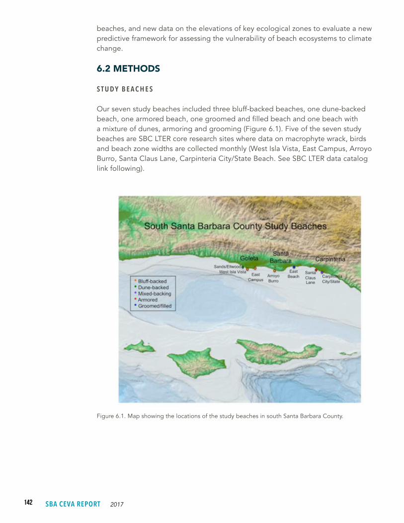
142 SBA CEVA REPORT 2017
beaches, and new data on the elevations of key ecological zones to evaluate a new predictive framework for assessing the vulnerability of beach ecosystems to climate change.
6.2 METHODS
S T U D Y B E A C H E S
Our seven study beaches included three bluff-backed beaches, one dune-backed beach, one armored beach, one groomed and filled beach and one beach with a mixture of dunes, armoring and grooming (Figure 6.1). Five of the seven study beaches are SBC LTER core research sites where data on macrophyte wrack, birds and beach zone widths are collected monthly (West Isla Vista, East Campus, Arroyo Burro, Santa Claus Lane, Carpinteria City/State Beach. See SBC LTER data catalog link following).
Figure 6.1. Map showing the locations of the study beaches in south Santa Barbara County.
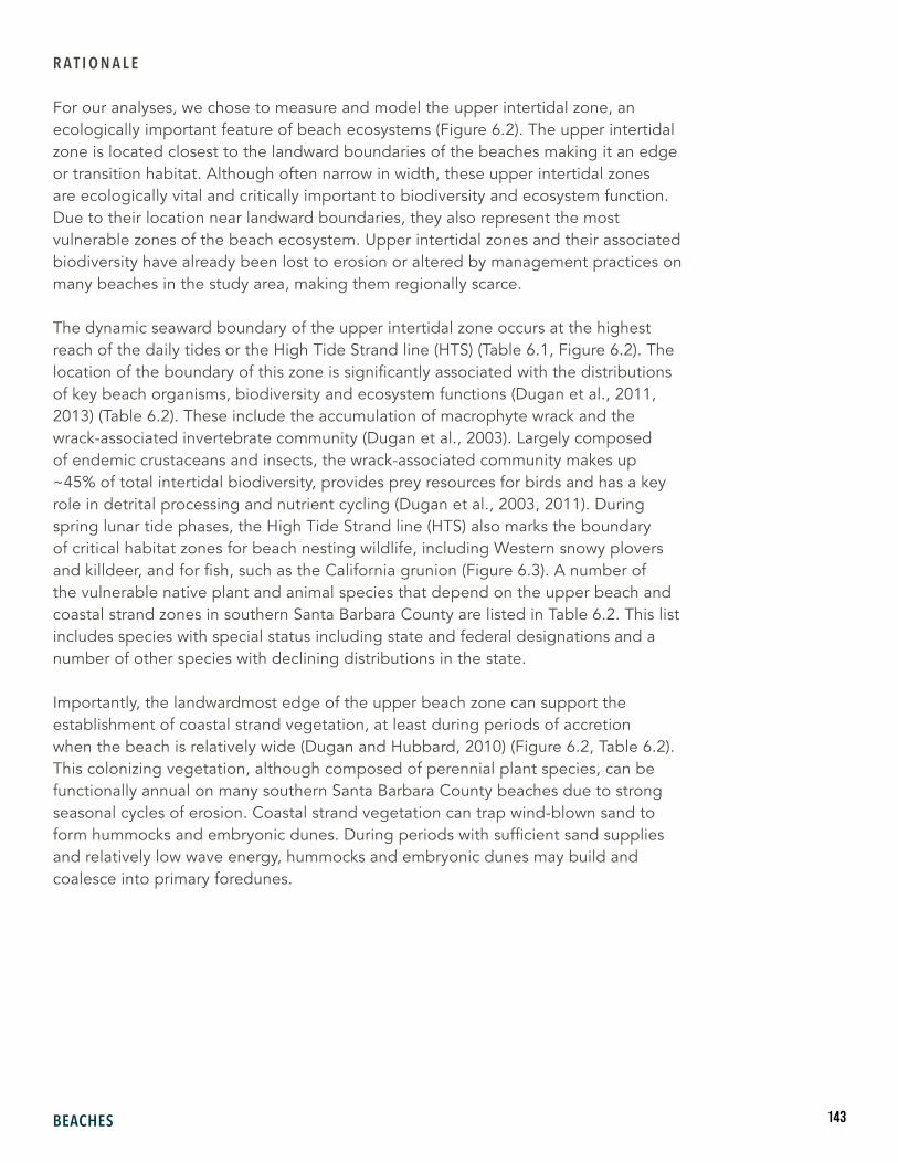
143BEACHES
R A T I O N A L E
For our analyses, we chose to measure and model the upper intertidal zone, an ecologically important feature of beach ecosystems (Figure 6.2). The upper intertidal zone is located closest to the landward boundaries of the beaches making it an edge or transition habitat. Although often narrow in width, these upper intertidal zones are ecologically vital and critically important to biodiversity and ecosystem function. Due to their location near landward boundaries, they also represent the most vulnerable zones of the beach ecosystem. Upper intertidal zones and their associated biodiversity have already been lost to erosion or altered by management practices on many beaches in the study area, making them regionally scarce.
The dynamic seaward boundary of the upper intertidal zone occurs at the highest reach of the daily tides or the High Tide Strand line (HTS) (Table 6.1, Figure 6.2). The location of the boundary of this zone is significantly associated with the distributions of key beach organisms, biodiversity and ecosystem functions (Dugan et al., 2011, 2013) (Table 6.2). These include the accumulation of macrophyte wrack and the wrack-associated invertebrate community (Dugan et al., 2003). Largely composed of endemic crustaceans and insects, the wrack-associated community makes up ~45% of total intertidal biodiversity, provides prey resources for birds and has a key role in detrital processing and nutrient cycling (Dugan et al., 2003, 2011). During spring lunar tide phases, the High Tide Strand line (HTS) also marks the boundary of critical habitat zones for beach nesting wildlife, including Western snowy plovers and killdeer, and for fish, such as the California grunion (Figure 6.3). A number of the vulnerable native plant and animal species that depend on the upper beach and coastal strand zones in southern Santa Barbara County are listed in Table 6.2. This list includes species with special status including state and federal designations and a number of other species with declining distributions in the state.
Importantly, the landwardmost edge of the upper beach zone can support the establishment of coastal strand vegetation, at least during periods of accretion when the beach is relatively wide (Dugan and Hubbard, 2010) (Figure 6.2, Table 6.2). This colonizing vegetation, although composed of perennial plant species, can be functionally annual on many southern Santa Barbara County beaches due to strong seasonal cycles of erosion. Coastal strand vegetation can trap wind-blown sand to form hummocks and embryonic dunes. During periods with sufficient sand supplies and relatively low wave energy, hummocks and embryonic dunes may build and coalesce into primary foredunes.
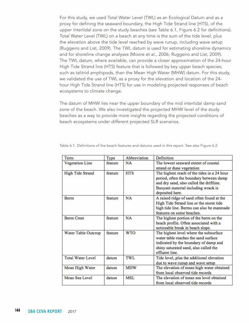
144 SBA CEVA REPORT 2017
Table 6.1. Definitions of the beach features and datums used in this report. See also Figure 6.2.
For this study, we used Total Water Level (TWL) as an Ecological Datum and as a proxy for defining the seaward boundary, the High Tide Strand line (HTS), of the upper intertidal zone on the study beaches (see Table 6.1, Figure 6.2 for definitions). Total Water Level (TWL) on a beach at any time is the sum of the tide level, plus the elevation above the tide level reached by wave runup, including wave setup (Ruggeiro and List, 2009). The TWL datum is used for estimating shoreline dynamics and for shoreline change analyses (Moore et al., 2006; Ruggeiro and List, 2009). The TWL datum, where available, can provide a closer approximation of the 24-hour High Tide Strand line (HTS) feature that is followed by key upper beach species, such as talitrid amphipods, than the Mean High Water (MHW) datum. For this study, we validated the use of TWL as a proxy for the elevation and location of the 24-hour High Tide Strand line (HTS) for use in modeling projected responses of beach ecosystems to climate change.
The datum of MHW lies near the upper boundary of the mid intertidal damp sand zone of the beach. We also investigated the projected MHW level of the study beaches as a way to provide more insights regarding the projected conditions of beach ecosystems under different projected SLR scenarios.
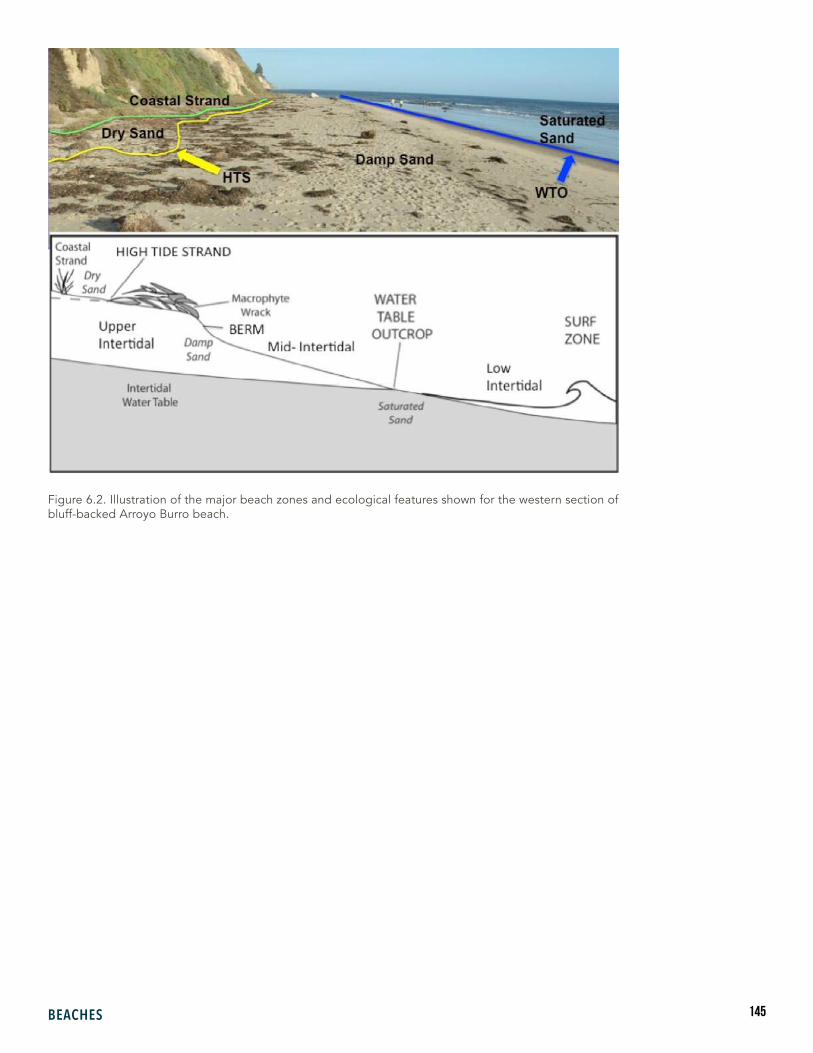
145BEACHES
Figure 6.2. Illustration of the major beach zones and ecological features shown for the western section of bluff-backed Arroyo Burro beach.
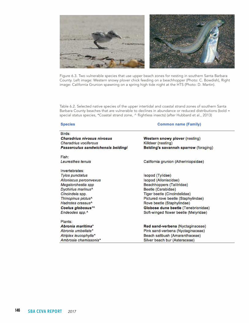
146 SBA CEVA REPORT 2017
Table 6.2. Selected native species of the upper intertidal and coastal strand zones of southern Santa Barbara County beaches that are vulnerable to declines in abundance or reduced distributions (bold = special status species, *Coastal strand zone, ^ flightless insects) (after Hubbard et al., 2013)
Figure 6.3. Two vulnerable species that use upper beach zones for nesting in southern Santa Barbara County. Left image: Western snowy plover chick feeding on a beachhopper (Photo: C. Bowdish), Right image: California Grunion spawning on a spring high tide night at the HTS (Photo: D. Martin).
147BEACHES
D A T A S O U R C E S
We used data on beach profiles, elevations, widths and coastal processes (Barnard et al., 2009; Griggs and Russell, 2011) combined with information we have collected on local beach ecosystems in previous studies (Dugan et al., 2003, 2008, 2011; Hubbard and Dugan, 2003) to develop a predictive framework of potential changes in intertidal features at selected beaches that represent the range of conditions present in the study area for several different sea level rise (SLR) scenarios (SLR 50 cm = 1.64 ft, 100 cm = 3.28 ft), 150 cm = 4.92 ft, 200 cm = 6.56 ft, and 500 cm = 16.4 ft).
Information on beaches for the SBA CEVA builds on existing research (USGS and SBC LTER and other studies) and new data collection. Detailed geo-referenced elevation data on beach profiles and evolution has been collected for the study area semi-annually since 2005 by Patrick Barnard’s team from USGS Pacific Coastal Science and Marine Science Center (See Barnard et al., 2017, Section 3 this report). Data from monthly surveys of ecological zone widths conducted on five of the study beaches on standard shore-normal transects has been collected by the SBC LTER since 2008 (see SBC LTER data catalog for data and protocols http://sbc.lternet.edu//data/dataCollectionsPortal.html).
Relationships between the distribution of key intertidal biota and beach features, such as the high tide strand (HTS), have been quantified for Santa Barbara County beaches (Dugan et al., 2013). We measured the elevations of these zones and additional biotic features including the vegetation line (the lowest extent of coastal strand vegetation) during USGS surveys of the study area beaches in order to expand the scope of our datasets. These physical and ecological data were integrated to develop ecologically relevant metrics that could be used as a basis for building a predictive framework for evaluating the vulnerability of beach ecosystems to sea level rise and climate change.
148 SBA CEVA REPORT 2017
BOX 5
Sandy beach ecosystems currently are not afforded the same level of protection as other important coastal ecosystems. Unlike coastal dunes, they are not designated by the state as environmentally sensitive habitat (ESHA). In state MPAs (Marine Protected Areas) the boundaries of many reserves extend only up to the mean high tide line. For beach ecosystems, where highly mobile species migrate across all of the beach zones to survive and >45% of the biodiversity lives above the mean high tide line, this leaves much of the most highly vulnerable biodiversity and function of beaches outside MPA protection. Interestingly, sandy beaches do meet the State of California’s wetland definition, although they are not currently recognized as such.
Coastal wetlands subject to regulation under the California Coastal Act are determined by the California Coastal Commission (CCC), with the assistance of the California Department of Fish and Wildlife (CDFW). The CDFW
Consider section 30121 of the California Coastal Act (1976). This statute, governing the California Coastal Commission (CCC), has a broad definition for a wetland:
“Wetland means lands within the coastal zone which may be covered periodically or permanently with shallow water and include saltwater marshes, freshwater marshes, open or closed brackish water marshes, swamps, mudflats, or fens.”
essentially relies on the federal wetland definition and classification system. However, a critically important difference in the CDFW wetland delineation process compared to the federal process, is that the state of California requires the presence of only one of the three attributes (hydrology, hydric soils, OR hydrophytic vegetation) for an area to qualify as a wetland. Although sandy beaches lack hydrophytes and well-developed hydric soils, by the CCC definition of coastal wetlands, the inundation regime (= hydrology) of sandy beaches could allow open coast sandy beach ecosystems to be classified as coastal wetlands in the State of California.
Designating beaches as coastal wetlands would provide a policy framework that could be broadly applied to help address conservation needs and the array of ongoing and anticipated impacts to beach ecosystems, including SLR and climate change.
SANDY BEACHES AS COASTAL WETLANDS
A LOOK AT THE LEGISLATION
A more explicit definition of coastal wetlands is provided by the CCC Administrative Regulations (Section 13577 (b)):
“Wetlands are lands where the water table is at, near, or above the land surface long enough to promote the formation of hydric soils or to support the growth of hydrophytes, and shall also include those types of wetlands where vegetation is lacking and soil is poorly developed or absent as a result of frequent or drastic fluctuations of surface water levels, wave action, water flow, turbidity or high concentrations of salt or other substance in the substrate. Such wetlands can be recognized by the presence of surface water or saturated substrate at some time during each year and their location within, or adjacent to, vegetated wetlands or deepwater habitats.”

149BEACHES
E C O L O G I C A L Z O N E S U R V E Y S
The elevations of the high tide strand (HTS) and the vegetation line (seawardmost extent of coastal strand vegetation) were surveyed by UCSB researchers at seven beaches in Santa Barbara County on one to four dates, depending on the beach site, between 2011 and 2015. Surveys were conducted by walking along the appropriate intertidal feature using a GPS backpack platform equipped with survey grade Trimble R7 and Topcon GRS-1 global navigation satellite system (GNSS) receivers with Zephyr 2 and PG-A1 antennas, respectively. The final positions were projected in Cartesian coordinates using the UTM Zone 11 North (meters) (NSRS 2007) coordinate system and NAVD88 orthometric elevations were computed using the National Geodetic Survey Geoid 12a.
The elevations of key ecological features from the high resolution GPS surveys of HTS and vegetation line features were used to evaluate the variation in the elevations of these features across beaches.
H I G H T I D E S T R A N D ( H T S ) A N D C O S M O S R U N U P E L E V A T I O N C O M P A R I S O N S
To validate the use of the TWL values generated by CoSMoS 3.0 in our projections of HTS elevations, the measured elevations of the HTS from field surveys were compared to the elevations of the maximum runup positions from the Coastal Storm Model System (CoSMoS) v3.0 Phase 2 Southern California Bight results (Erikson et al., 2017). The CoSMoS runup elevations were located at cross-shore transects (CSTs) spaced 100 meters apart alongshore and represent two sea-state simulations: ambient or daily and one-year/annual storm conditions (See Figure 6.9a-g). The average HTS elevation in the region surrounding each CST was calculated using ArcMap 10.2. The HTS elevations for each survey and the CoSMoS runup elevations were plotted using Matlab R2015b.
B E A C H Z O N E W I D T H C O M P A R I S O N S
Mean values for beach zone widths measured during field surveys of the study beaches by the SBC LTER (http://sbc.lternet.edu//data/dataCollectionsPortal.html) (http://sbc.lternet.edu/cgi-bin/showDataset.cgi?docid=knb-lter-sbc.40) were compared to projected widths from CoSMoS v3.0 Phase 2 Southern California Bight results for 2010, SLR = 0 conditions.
R U N U P P R O J E C T I O N S
Projections of changes in upper beach zone widths under different SLR levels were generated by CoSMoS 3.0. The CoSMoS runup (TWL) outputs for ambient and one-year/annual storm conditions were used as a proxy for the location of the HTS under future sea level conditions, allowing for an estimate of the upper beach zone width, the area between the HTS and landward extent of the sandy beach. The distance from the back beach location, defined by the CoSMoS non-erodible shoreline, to the
150 SBA CEVA REPORT 2017
runup point along each cross-shore transect (CST) was measured using ArcMap 10.2 and Matlab R2015b. The same method was used to measure the distance from the back beach to the location of the CoSMoS projected shoreline, represented by the mean high water (MHW) elevation. In some bluff-backed areas, the upper beach zone width was instead estimated using the location of the CoSMoS projected mean high water shoreline when its location was landward of the runup projection. In certain locations where the CoSMoS model did not produce a runup position, the upper beach zone width was interpolated based on adjacent CSTs, as well as the preceding and successive sea level conditions.
6.3 RESULTS/DISCUSSION
C U R R E N T C O N D I T I O N S
The majority of beaches in southern Santa Barbara County (78%, 83 km) are backed by fairly resistant sea bluffs that provide relatively little scope for shoreline retreat. Many of these beaches lose sand during the winter and spring, exposing wave-cut bedrock platforms. A number of small pocket beaches associated with creek and stream mouths, which can seasonally impound and form small lagoons behind the beach berm, break up the nearly continuous stretch of bluff-backed beaches (e.g., Gaviota, Refugio, Haskells, Arroyo Burro). Dune-backed beaches with greater potential for retreat are now very limited in extent. Historically up to 19% (14.6 km, 9 miles) of sandy beaches were backed by coastal dunes in southern Santa Barbara County. Dune-backed beaches are or were formerly associated with the major structural basins of Devereux Slough, Goleta Slough, Mission Creek, and Carpinteria Salt Marsh and Carpinteria Creek. However, of these, the only remaining unarmored and/or undeveloped dune-backed beaches are Sands Beach located at the mouth of Devereux Slough and a stretch of Carpinteria State Beach, just west of Carpinteria Creek, making up only 3% (~2.4 km, 1.5 miles) of the region’s beaches. Sands Beach is oriented to the southwest, and can receive strong westerly winds that promote aeolian sand transport and dune building. All the other formerly dune-backed beaches in the region are now bounded by coastal development, such as parking lots, recreational facilities, parks, roads, houses, rock revetments and seawalls.
The sandy beach ecosystems of our Santa Barbara study area represent a range of conditions from relatively unaltered and undeveloped to highly urbanized and managed. The beaches are subject to very different levels of disturbance and management, ranging from highly manipulated beaches that are impacted by grooming, armoring and mechanical berm building to unmanaged beaches in relatively undisturbed condition. Major coastal development is present in the cities of Santa Barbara and Carpinteria and stretches of coastal armoring are associated with the railroad along even remote sections of the study coastline. Human alteration, including development or coastal armoring affects ~24% (19 km, 11.8 miles) of the sandy beaches (both bluff- and dune-backed) in southern Santa Barbara County; of this 5% (~4 km, 2.5 miles) of the beaches are groomed, and 19% (~15.5 km, 9.6 miles) are armored.

151BEACHES
The bluff- and dune-backed beaches of the study area that have remained largely unmanaged and undeveloped provide a wide variety of ecosystem functions and services (Schlacher et al., 2008; Defeo et al., 2009). These beaches currently support remarkably rich intertidal food webs that provide valuable prey resources to large numbers of wintering and resident shorebirds, including endangered and declining species (Dugan et al., 2003; Hubbard and Dugan, 2003), as well as surf zone fish. These beaches are vital as nesting habitat for birds and fish, including the Western snowy plover and the California grunion (Figure 6.3). In contrast, the groomed and many of the armored beaches in the study area currently support impoverished intertidal food webs, particularly the wrack-dependent upper intertidal zone component (Dugan et al., 2003; Dugan et al., 2008).
Beach features, including presence, overall and intertidal zone widths, distributions and elevations, vary across the study beaches. Overall mean widths of intertidal zones ranged from 50 to 90 m (164-295 ft), while mean widths of upper beach zones (dry) ranged from 8 to 20 m (26-65 ft) (Figure 6.4).
Figure 6.4. Relative distribution of average intertidal zones expressed as widths on four south Santa Barbara County beaches (n = 24, monthly low tide surveys December 2011– November 2013 data from Dugan et al., 2015). The boundary between damp and dry sand zones is the high tide strand line (HTS) that we are approximating with projected Total Water Levels, TWL, from CoSMoS 3.0. Note 1 meter = 3.28 feet.
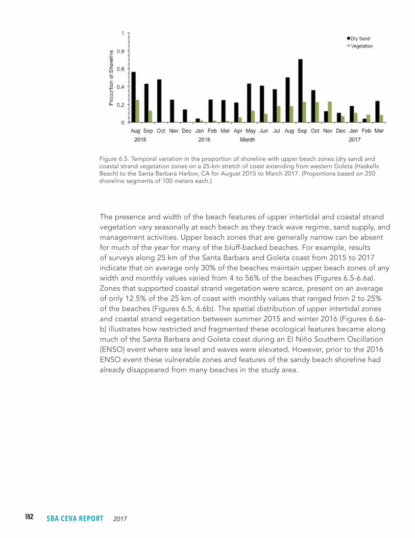
152 SBA CEVA REPORT 2017
Figure 6.5. Temporal variation in the proportion of shoreline with upper beach zones (dry sand) and coastal strand vegetation zones on a 25-km stretch of coast extending from western Goleta (Haskells Beach) to the Santa Barbara Harbor, CA for August 2015 to March 2017. (Proportions based on 250 shoreline segments of 100 meters each.)
The presence and width of the beach features of upper intertidal and coastal strand vegetation vary seasonally at each beach as they track wave regime, sand supply, and management activities. Upper beach zones that are generally narrow can be absent for much of the year for many of the bluff-backed beaches. For example, results of surveys along 25 km of the Santa Barbara and Goleta coast from 2015 to 2017 indicate that on average only 30% of the beaches maintain upper beach zones of any width and monthly values varied from 4 to 56% of the beaches (Figures 6.5-6.6a). Zones that supported coastal strand vegetation were scarce, present on an average of only 12.5% of the 25 km of coast with monthly values that ranged from 2 to 25% of the beaches (Figures 6.5, 6.6b). The spatial distribution of upper intertidal zones and coastal strand vegetation between summer 2015 and winter 2016 (Figures 6.6a-b) illustrates how restricted and fragmented these ecological features became along much of the Santa Barbara and Goleta coast during an El Niño Southern Oscillation (ENSO) event where sea level and waves were elevated. However, prior to the 2016 ENSO event these vulnerable zones and features of the sandy beach shoreline had already disappeared from many beaches in the study area.
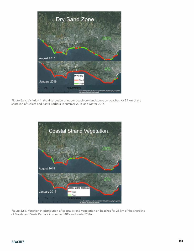
153BEACHES
Figure 6.6a. Variation in the distribution of upper beach dry sand zones on beaches for 25 km of the shoreline of Goleta and Santa Barbara in summer 2015 and winter 2016.
Figure 6.6b. Variation in distribution of coastal strand vegetation on beaches for 25 km of the shoreline of Goleta and Santa Barbara in summer 2015 and winter 2016.
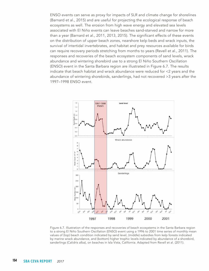
154 SBA CEVA REPORT 2017
Figure 6.7. Illustration of the responses and recoveries of beach ecosystems in the Santa Barbara region to a strong El Niño Southern Oscillation (ENSO) event using a 1996 to 2001 time series of monthly mean values of (top) beach condition indicated by sand level, (middle) subsidies from kelp forests indicated by marine wrack abundance, and (bottom) higher trophic levels indicated by abundance of a shorebird, sanderlings (Calidris alba), on beaches in Isla Vista, California. Adapted from Revell et al. (2011).
ENSO events can serve as proxy for impacts of SLR and climate change for shorelines (Barnard et al., 2015) and are useful for projecting the ecological response of beach ecosystems as well. The erosion from high wave energy and elevated sea levels associated with El Niño events can leave beaches sand-starved and narrow for more than a year (Barnard et al., 2011, 2013, 2015). The significant effects of these events on the distribution of upper beach zones, nearshore kelp beds and wrack inputs, the survival of intertidal invertebrates, and habitat and prey resources available for birds can require recovery periods stretching from months to years (Revell et al., 2011). The responses and recoveries of the beach ecosystem components of sand levels, wrack abundance and wintering shorebird use to a strong El Niño Southern Oscillation (ENSO) event in the Santa Barbara region are illustrated in Figure 6.7. The results indicate that beach habitat and wrack abundance were reduced for <2 years and the abundance of wintering shorebirds, sanderlings, had not recovered >3 years after the 1997–1998 ENSO event.
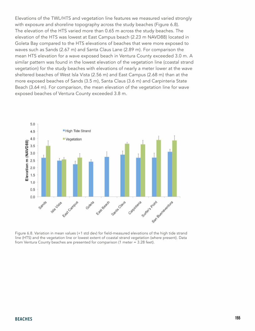
155BEACHES
Figure 6.8. Variation in mean values (+1 std dev) for field-measured elevations of the high tide strand line (HTS) and the vegetation line or lowest extent of coastal strand vegetation (where present). Data from Ventura County beaches are presented for comparison (1 meter = 3.28 feet).
Elevations of the TWL/HTS and vegetation line features we measured varied strongly with exposure and shoreline topography across the study beaches (Figure 6.8). The elevation of the HTS varied more than 0.65 m across the study beaches. The elevation of the HTS was lowest at East Campus beach (2.23 m NAVD88) located in Goleta Bay compared to the HTS elevations of beaches that were more exposed to waves such as Sands (2.67 m) and Santa Claus Lane (2.89 m). For comparison the mean HTS elevation for a wave exposed beach in Ventura County exceeded 3.0 m. A similar pattern was found in the lowest elevation of the vegetation line (coastal strand vegetation) for the study beaches with elevations of nearly a meter lower at the wave sheltered beaches of West Isla Vista (2.56 m) and East Campus (2.68 m) than at the more exposed beaches of Sands (3.5 m), Santa Claus (3.6 m) and Carpinteria State Beach (3.64 m). For comparison, the mean elevation of the vegetation line for wave exposed beaches of Ventura County exceeded 3.8 m.

156 SBA CEVA REPORT 2017
V A L I D A T I O N O F C O S M O S 3 . 0 M O D E L R E S U L T S W I T H F I E L D V A L U E S
Our validations showed generally good coherence between the CoSMos modeling projections (SLR = 0) and our field-measured values. The locations of the CoSMoS cross-shore transects (CSTs) and the erosion boundary used in the model projections are shown for each study beach in aerial views (Figures 6.9a-g). The erosion boundary set as a CoSMoS 3.0 model parameter is illustrated as a red line in each aerial image. This line marks the limit of shoreline retreat and hence the scope of beach width change possible in the model outputs. Each aerial image is aligned with the CoSMoS model results for projected beach zone widths for SLR = 0 using beach profiles from 2010 (Figures 6.9a-g).
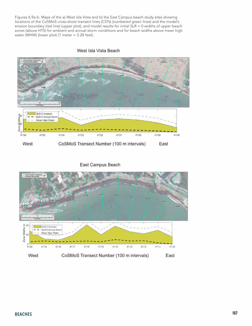
157BEACHES
Figures 6.9a-b. Maps of the a) West Isla Vista and b) the East Campus beach study sites showing locations of the CoSMoS cross-shore transect lines (CSTs) (numbered green lines) and the model’s erosion boundary (red line) (upper plot), and model results for initial SLR = 0 widths of upper beach zones (above HTS) for ambient and annual storm conditions and for beach widths above mean high water (MHW) (lower plot) (1 meter = 3.28 feet).
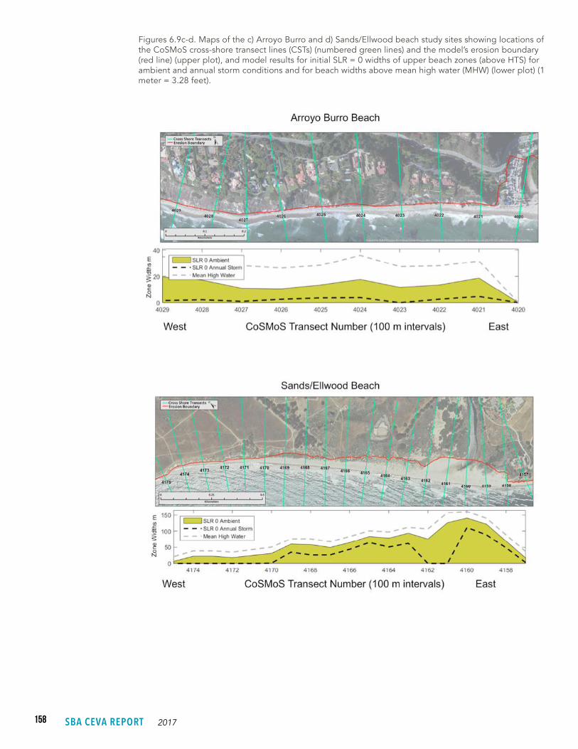
158 SBA CEVA REPORT 2017
Figures 6.9c-d. Maps of the c) Arroyo Burro and d) Sands/Ellwood beach study sites showing locations of the CoSMoS cross-shore transect lines (CSTs) (numbered green lines) and the model’s erosion boundary (red line) (upper plot), and model results for initial SLR = 0 widths of upper beach zones (above HTS) for ambient and annual storm conditions and for beach widths above mean high water (MHW) (lower plot) (1 meter = 3.28 feet).

159BEACHES
Figures 6.9e-f. Maps of the e) Santa Claus Lane and f) Carpinteria City and State Beach study sites showing locations of the CoSMoS cross-shore transect lines (CSTs) (numbered green lines) and the model’s erosion boundary (red line) (upper plot) and model results for initial SLR = 0 widths of upper beach zones (above HTS) for ambient and annual storm conditions and for beach widths above mean high water (MHW) (lower plot) (1 meter = 3.28 feet).

160 SBA CEVA REPORT 2017
Figure 6.9g. Map of the East Beach study site showing locations of the CoSMoS cross shore transect lines (CSTs) (numbered green lines) and the model’s erosion boundary (red line) (upper plot) and model results for initial SLR = 0 widths of upper beach zones (above HTS) for ambient and annual storm conditions and for beach widths above mean high water (MHW) (lower plot) (1 meter = 3.28 feet).

161BEACHES
There was excellent agreement between the mean values of upper beach zone widths projected by CoSMoS and the field-measured values (2008–2014) at the four core SBC-LTER and CEVA study beaches used for this analyses (Figure 6.10a). The CoSMoS projected elevations for TWL (SLR = 0) for ambient and 1-year storm conditions bracketed the field measured HTS elevations at four of the study beaches (Figure 6.10b). However, for three of the study beaches, the annual storm projections of TWL elevations were equal to or slightly lower than the field-measured HTS values (Figures 6.10a-b).
Figure 6.10a. Comparison of mean values of projected dry beach zone widths (+1 std dev) (zone above HTS/TWL) for SLR = 0 from CoSMoS 3.0 model results for ambient conditions and the mean values (+1 std dev) from monthly SBC LTER beach monitoring for a subset of the CEVA study beaches. Note 1 meter = 3.28 feet.
Figure 6.10b. Comparison of mean values (+1 std dev) of projected elevations for TWL in ambient and annual storm conditions for SLR = 0 from CoSMoS 3.0 model results and the mean values (+1 std dev) of elevations for HTS measured in the field at the study beaches. Note: 1 meter = 3.28 feet.
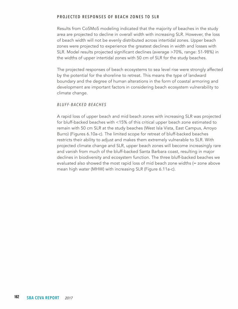
162 SBA CEVA REPORT 2017
P R O J E C T E D R E S P O N S E S O F B E A C H Z O N E S T O S L R
Results from CoSMoS modeling indicated that the majority of beaches in the study area are projected to decline in overall width with increasing SLR. However, the loss of beach width will not be evenly distributed across intertidal zones. Upper beach zones were projected to experience the greatest declines in width and losses with SLR. Model results projected significant declines (average >70%, range: 51-98%) in the widths of upper intertidal zones with 50 cm of SLR for the study beaches.
The projected responses of beach ecosystems to sea level rise were strongly affected by the potential for the shoreline to retreat. This means the type of landward boundary and the degree of human alterations in the form of coastal armoring and development are important factors in considering beach ecosystem vulnerability to climate change.
B L U F F - B A C K E D B E A C H E S
A rapid loss of upper beach and mid beach zones with increasing SLR was projected for bluff-backed beaches with <15% of this critical upper beach zone estimated to remain with 50 cm SLR at the study beaches (West Isla Vista, East Campus, Arroyo Burro) (Figures 6.10a-c). The limited scope for retreat of bluff-backed beaches restricts their ability to adjust and makes them extremely vulnerable to SLR. With projected climate change and SLR, upper beach zones will become increasingly rare and vanish from much of the bluff-backed Santa Barbara coast, resulting in major declines in biodiversity and ecosystem function. The three bluff-backed beaches we evaluated also showed the most rapid loss of mid beach zone widths (= zone above mean high water (MHW) with increasing SLR (Figure 6.11a-c).

163BEACHES
Figure 6.11a. CoSMoS 3.0 model projections of beach zone widths above TWL for ambient conditions and annual storm conditions, and above MHW under SLR = 0 under no SLR and SLR levels ranging from 50 to 500 cm for the bluff-backed beach at Arroyo Burro (SLR 50 cm = 1.64 ft, 100 cm = 3.28 ft, 150 cm = 4.92 ft, 200 cm = 6.56 ft, and 500 cm = 16.4 ft).
With 50 cm of SLR, the narrowest bluff-backed beach, Arroyo Burro, was projected to lose >90% of upper beach zone width and retain only a very narrow (<1 m) upper beach zone on less than half of the shoreline segment we analyzed (Figure 6.11a). The damp beach above MHW was projected to be maintained for much of the beach segment with 50 cm SLR but with 100 cm of SLR it disappeared from the majority (66%) of the beach segment.
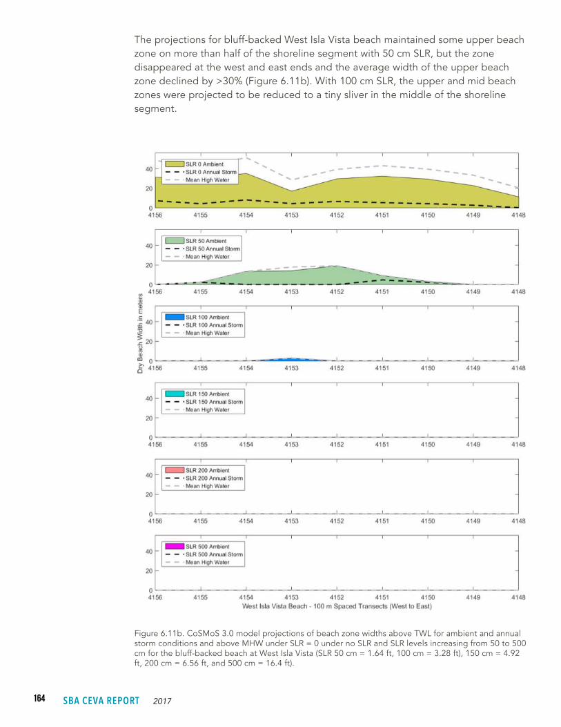
164 SBA CEVA REPORT 2017
The projections for bluff-backed West Isla Vista beach maintained some upper beach zone on more than half of the shoreline segment with 50 cm SLR, but the zone disappeared at the west and east ends and the average width of the upper beach zone declined by >30% (Figure 6.11b). With 100 cm SLR, the upper and mid beach zones were projected to be reduced to a tiny sliver in the middle of the shoreline segment.
Figure 6.11b. CoSMoS 3.0 model projections of beach zone widths above TWL for ambient and annual storm conditions and above MHW under SLR = 0 under no SLR and SLR levels increasing from 50 to 500 cm for the bluff-backed beach at West Isla Vista (SLR 50 cm = 1.64 ft, 100 cm = 3.28 ft), 150 cm = 4.92 ft, 200 cm = 6.56 ft, and 500 cm = 16.4 ft).
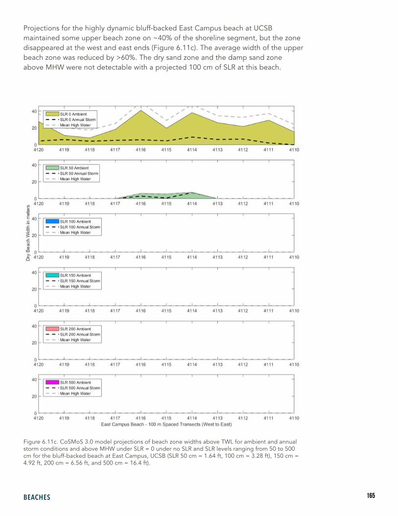
165BEACHES
Projections for the highly dynamic bluff-backed East Campus beach at UCSB maintained some upper beach zone on ~40% of the shoreline segment, but the zone disappeared at the west and east ends (Figure 6.11c). The average width of the upper beach zone was reduced by >60%. The dry sand zone and the damp sand zone above MHW were not detectable with a projected 100 cm of SLR at this beach.
Figure 6.11c. CoSMoS 3.0 model projections of beach zone widths above TWL for ambient and annual storm conditions and above MHW under SLR = 0 under no SLR and SLR levels ranging from 50 to 500 cm for the bluff-backed beach at East Campus, UCSB (SLR 50 cm = 1.64 ft, 100 cm = 3.28 ft), 150 cm = 4.92 ft, 200 cm = 6.56 ft, and 500 cm = 16.4 ft).

166 SBA CEVA REPORT 2017
D U N E - B A C K E D B E A C H E S
Dune-backed beaches, such as the beach at Sands/Ellwood, were projected to have the greatest resilience to increasing SLR for upper and mid intertidal zones, maintaining narrow zones of upper (9%) and mid-intertidal habitats even with 200 cm SLR (Figure 6.11d). However even this dune-backed beach lost >60% of the width of the upper beach zone with 50 cm of SLR. Note: The model sets an erosion boundary that limits the scope of projected retreat even for dune-backed beaches.
Figure 6.11d. CoSMoS 3.0 model projections of beach zone widths above TWL for ambient conditions and annual storm conditions and above MHW under SLR = 0 under no SLR and SLR levels ranging from 50-500 cm for the dune-backed beach at Sands/Ellwood(SLR 50 cm = 1.64 ft, 100 cm = 3.28 ft), 150 cm = 4.92 ft, 200 cm = 6.56 ft, and 500 cm = 16.4 ft).
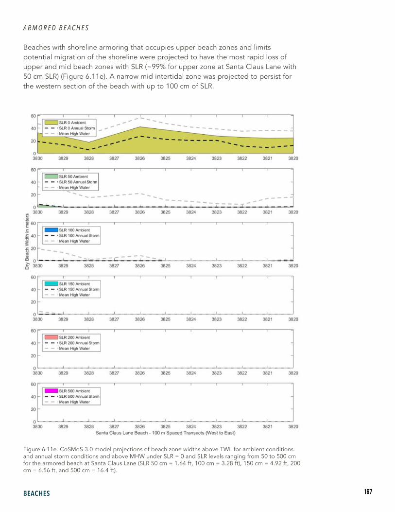
167BEACHES
A R M O R E D B E A C H E S
Beaches with shoreline armoring that occupies upper beach zones and limits potential migration of the shoreline were projected to have the most rapid loss of upper and mid beach zones with SLR (~99% for upper zone at Santa Claus Lane with 50 cm SLR) (Figure 6.11e). A narrow mid intertidal zone was projected to persist for the western section of the beach with up to 100 cm of SLR.
Figure 6.11e. CoSMoS 3.0 model projections of beach zone widths above TWL for ambient conditions and annual storm conditions and above MHW under SLR = 0 and SLR levels ranging from 50 to 500 cm for the armored beach at Santa Claus Lane (SLR 50 cm = 1.64 ft, 100 cm = 3.28 ft), 150 cm = 4.92 ft, 200 cm = 6.56 ft, and 500 cm = 16.4 ft).
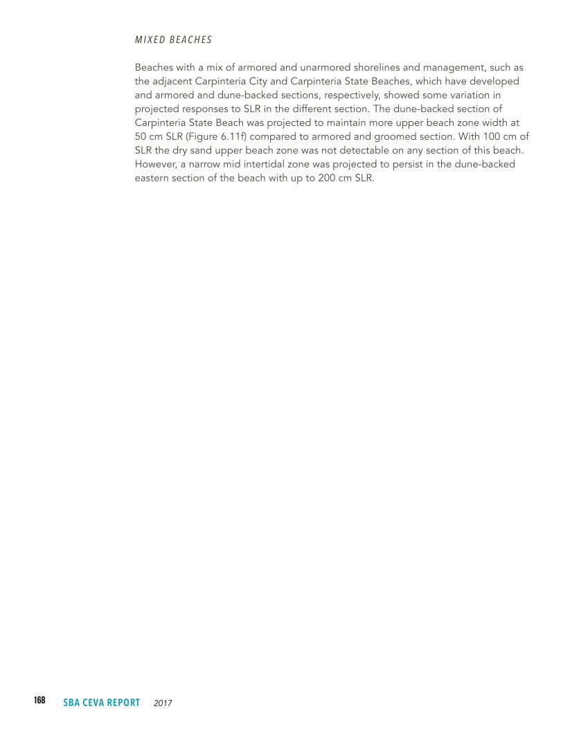
168 SBA CEVA REPORT 2017
M I X E D B E A C H E S
Beaches with a mix of armored and unarmored shorelines and management, such as the adjacent Carpinteria City and Carpinteria State Beaches, which have developed and armored and dune-backed sections, respectively, showed some variation in projected responses to SLR in the different section. The dune-backed section of Carpinteria State Beach was projected to maintain more upper beach zone width at 50 cm SLR (Figure 6.11f) compared to armored and groomed section. With 100 cm of SLR the dry sand upper beach zone was not detectable on any section of this beach. However, a narrow mid intertidal zone was projected to persist in the dune-backed eastern section of the beach with up to 200 cm SLR.
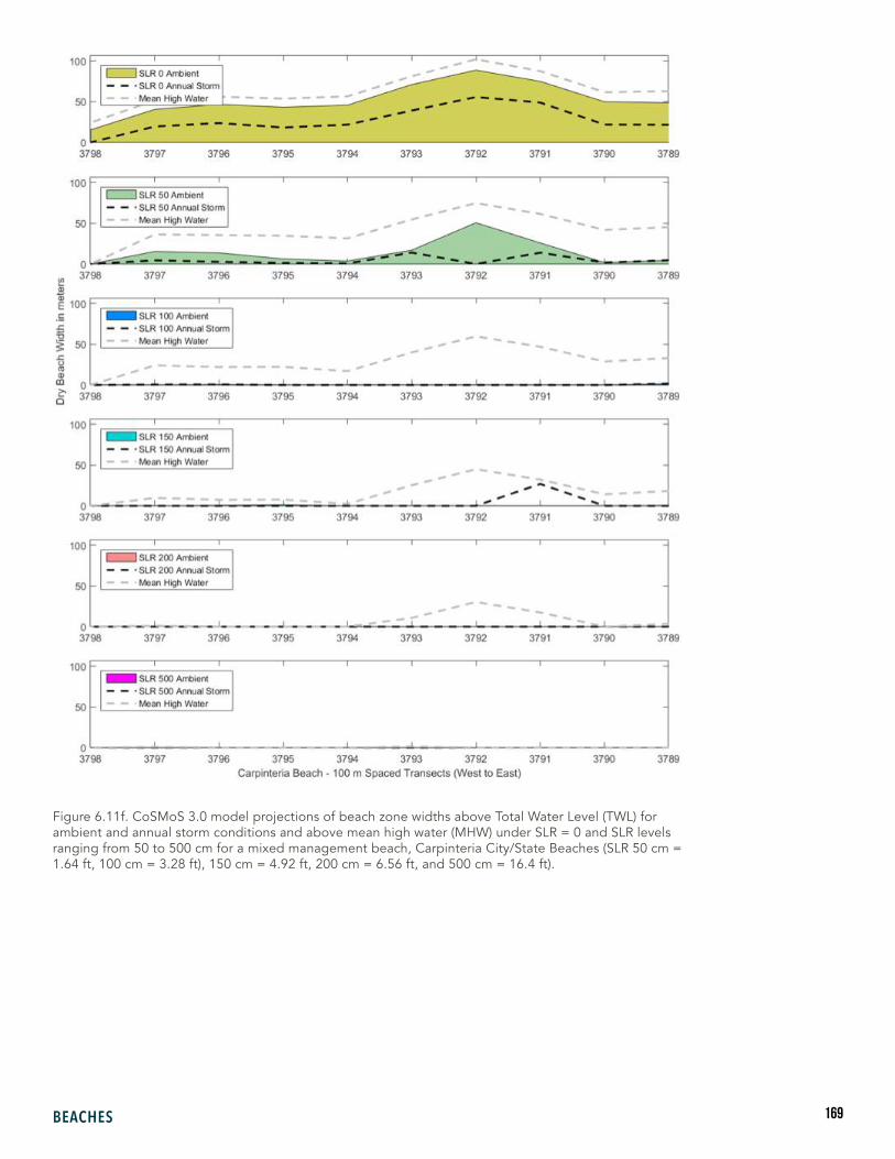
169BEACHES
Figure 6.11f. CoSMoS 3.0 model projections of beach zone widths above Total Water Level (TWL) for ambient and annual storm conditions and above mean high water (MHW) under SLR = 0 and SLR levels ranging from 50 to 500 cm for a mixed management beach, Carpinteria City/State Beaches (SLR 50 cm = 1.64 ft, 100 cm = 3.28 ft), 150 cm = 4.92 ft, 200 cm = 6.56 ft, and 500 cm = 16.4 ft).

170 SBA CEVA REPORT 2017
Figure 6.11g. CoSMoS 3.0 model projections of beach zone widths above TWL for ambient conditions and annual storm conditions and above MHW under SLR = 0 and SLR levels ranging from 50 to 500 cm for a groomed and filled beach, East Beach scenarios (SLR 50 cm = 1.64 ft, 100 cm = 3.28 ft), 150 cm = 4.92 ft, 200 cm = 6.56 ft, and 500 cm = 16.4 ft)

171BEACHES
B E A C H E S M A N A G E D F O R R E C R E A T I O N
East Beach, which has an artificially wide upper intertidal zone associated with beach grooming and filling, was also projected to have some resilience to SLR but still lost >50% of the upper beach zone width with 50 cm SLR (Figure 6.11g). Regular mechanized grooming inhibits the development of coastal strand and dune vegetation above the reach of tides and the beach fills from harbor dredging periodically increase the width of the beach. The behavior of this beach under SLR reflects the retreat of the intertidal beach into the wide unvegetated and degraded dune zone created by the combination of grooming and filling activities. This beach was projected to maintain some width in the upper beach zone for much of the shoreline segment for both 50 and 100 cm SLR, but with 150 cm SLR the upper beach zone was projected to shrink to <5 m.
The current management of East Beach and other groomed urban beaches, such as Ledbetter, West Beach and Carpinteria City Beach, has resulted in greatly impoverished intertidal biota, a lack of resilient dunes and reduced ecological function (Dugan et al., 2003; Dugan and Hubbard, 2010; Schooler et al., 2017). However, this model result suggests that exploring opportunities to restore biodiversity, coastal dunes and ecosystem function of these degraded but relatively wide beaches could potentially enhance the conservation of vulnerable beach ecosystems under SLR in the study area and elsewhere. Altering management practices to allow the recovery and restoration of more natural features, such as dunes and sand-trapping vegetation, on these currently degraded beaches could enhance their resilience to SLR from climate change and provide potential conservation benefits for vulnerable upper beach biota (Table 6.2) and coastal biodiversity.
S U M M A R Y
A summary of the projected mean values for widths for upper beach dry sand zones and mid/damp beach zones illustrates the magnitude of projected losses of beach habitat zones on beaches of all types with increasing SLR in southern Santa Barbara County (Figures 6.12a-c). With 50 cm of SLR, the model projections suggest even damp sand zones would be greatly reduced (<10 m) for bluff-backed beaches.
A rapid loss of upper beach and mid beach zones with increasing SLR was projected for bluff-backed beaches with <15% of the critical upper beach zone estimated to remain with 50 cm SLR (1.64 ft) at the bluff-backed study beaches (West Isla Vista, East Campus, Arroyo Burro) (Figure 6.12c). The limited scope for retreat of bluff-backed beaches restricts their ability to adjust and makes them extremely vulnerable to SLR. Bluff-backed beaches dominate the coastline of southern Santa Barbara County. With projected climate change and SLR, upper beach zones are projected to become increasingly rare and vanish from majority of the Santa Barbara coast, resulting in major declines in biodiversity and ecosystem function.
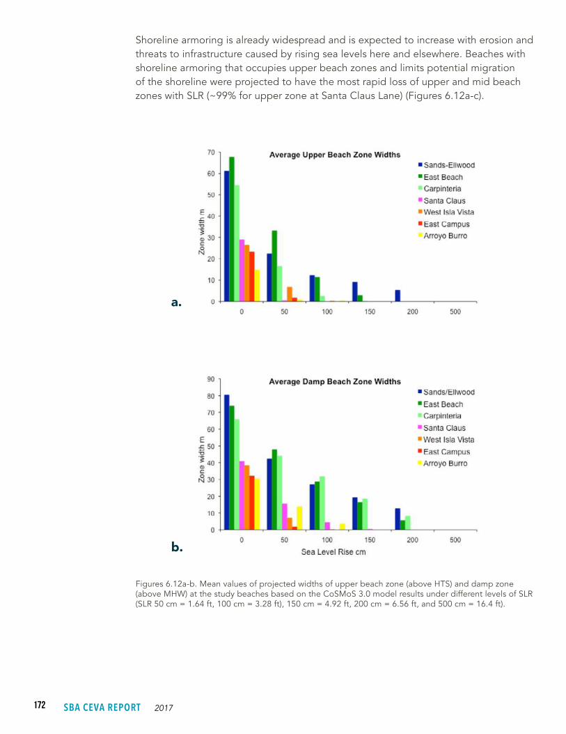
172 SBA CEVA REPORT 2017
Shoreline armoring is already widespread and is expected to increase with erosion and threats to infrastructure caused by rising sea levels here and elsewhere. Beaches with shoreline armoring that occupies upper beach zones and limits potential migration of the shoreline were projected to have the most rapid loss of upper and mid beach zones with SLR (~99% for upper zone at Santa Claus Lane) (Figures 6.12a-c).
Figures 6.12a-b. Mean values of projected widths of upper beach zone (above HTS) and damp zone (above MHW) at the study beaches based on the CoSMoS 3.0 model results under different levels of SLR (SLR 50 cm = 1.64 ft, 100 cm = 3.28 ft), 150 cm = 4.92 ft, 200 cm = 6.56 ft, and 500 cm = 16.4 ft).
a.
b.
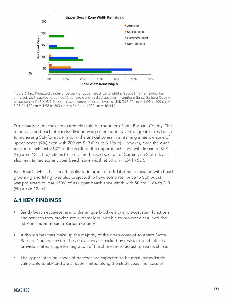
173BEACHES
Dune-backed beaches are extremely limited in southern Santa Barbara County. The dune-backed beach at Sands/Ellwood was projected to have the greatest resilience to increasing SLR for upper and mid intertidal zones, maintaining a narrow zone of upper beach (9%) even with 200 cm SLR (Figure 6.12a-b). However, even the dune-backed beach lost >60% of the width of the upper beach zone with 50 cm of SLR (Figure 6.12c). Projections for the dune-backed section of Carpinteria State Beach also maintained some upper beach zone width at 50 cm (1.64 ft) SLR.
East Beach, which has an artificially wide upper intertidal zone associated with beach grooming and filling, was also projected to have some resilience to SLR but still was projected to lose >50% of its upper beach zone width with 50 cm (1.64 ft) SLR (Figures 6.12a-c).
6.4 KEY FINDINGS
• Sandy beach ecosystems and the unique biodiversity and ecosystem functions and services they provide are extremely vulnerable to projected sea level rise (SLR) in southern Santa Barbara County.
• Although beaches make up the majority of the open coast of southern Santa Barbara County, most of these beaches are backed by resistant sea bluffs that provide limited scope for migration of the shoreline to adjust to sea level rise.
• The upper intertidal zones of beaches are expected to be most immediately vulnerable to SLR and are already limited along the study coastline. Loss of
Figure 6.12c. Projected values of percent of upper beach zone widths (above HTS) remaining for armored, bluff-backed, groomed/filled, and dune-backed beaches in southern Santa Barbara County based on the CoSMoS 3.0 model results under different levels of SLR (SLR 50 cm = 1.64 ft, 100 cm = 3.28 ft), 150 cm = 4.92 ft, 200 cm = 6.56 ft, and 500 cm = 16.4 ft).
c.

174 SBA CEVA REPORT 2017
these zones will strongly impact the wrack-associated biota, reducing intertidal biodiversity by 40-50%, decreasing the prey available for birds and fish and eliminating nesting habitat for species of concern (California grunion and Western snowy plover). Loss of these zones will also affect the existence of sand-trapping coastal strand vegetation, sand accumulation and nutrient cycling and greatly diminish the buffer areas required by the mobile intertidal animals of lower intertidal zones to survive high waves and storm conditions.
• With 50 cm (1.64 ft) of SLR the model results projected significant declines (average >70%, range 51-98%) in the widths of upper intertidal zones for all the study beaches. This is projected to occur by 2070 or earlier if GHG emissions continue as usual (Sections 2 and 4).
• The projected responses of beach ecosystems to sea level rise were strongly affected by the potential for the shoreline to retreat or migrate. The type of landward boundary, including coastal armoring and development, affects vulnerability of beach ecosystems to SLR.
• With projected climate change and SLR, upper beach zones that are already on the edge will become increasingly rare and vanish from much of the bluff-backed sandy beach shoreline of southern Santa Barbara County. On bluff-backed beaches, the model predicts a significant loss of this critical habitat zone will manifest with as little as 50 cm (1.64 ft) SLR .
• Beaches with shoreline armoring that occupies upper beach zones and limits migration of the shoreline were projected to have the most rapid loss of upper and mid beach zones with SLR.
• Dune-backed beaches were projected to have greater resilience to SLR. For the unconstrained beaches of Sands and Ellwood, the retreat of the shoreline into dune habitat allowed at least narrow upper beach zones to be maintained with up to 200 cm (6.58 ft) of SLR.
• The dominance of bluff-backed beaches along the coast means options for preserving beach ecosystems are limited to beaches that have some scope for retreat. These include groomed and filled beaches that are currently managed primarily for recreation.
• Restoring the biodiversity, dunes and ecosystem function of intensively managed beaches that are currently degraded yet relatively wide could provide opportunities for conservation of vulnerable beach ecosystems with SLR.
• Allowing more of the sand from streams and watersheds to enter the littoral cell could provide additional scope for conserving beach ecosystems with SLR in southern Santa Barbara County.
Callie B
owd
ish

7. Take Home MessagesCLIMATE CHANGE PROJECTIONS
• All climate models examined were consistent in predicting increasing temperatures across Santa Barbara County throughout the 21st century. Averaging over 10 climate models using the RCP 8.5 emissions scenarios, the projected temperature increases were about 1.5°F by 2030, 3°F by 2050, and 6-7°F by 2090. The temperature increases were more pronounced in the inland and mountain areas of the county and less along the coast and offshore islands.
• The number of extremely hot days (as measured by current 99th percentile historical values) in Santa Barbara County is projected to increase significantly with more than a doubling by 2050 and a nearly 10-fold increase by 2090. These projected changes would very likely increase the stress placed upon many vulnerable ecosystems.
175
Callie B
owd
ish
SBA CEVA REPORT 2017
• There is considerable spread in projected precipitation with all models having great year-to-year and even decade-to-decade variations, similar to historical behavior. The median annual precipitation from the 10 model projections yielded little change, suggesting that average annual precipitation may remain at historical levels during the 21st century. However, the individual models produced inconsistent projections of annual precipitation with some showing reduced and others increased amounts relative to historical average. As a result, there is considerable uncertainty in Santa Barbara County precipitation changes.
• The model projections are more consistent regarding changes in frequency and variability of future precipitation, especially during the latter half of the 21st
century. The models predict fewer but more intense storms, a reduction in the number of wet (rainy) days, and a decrease in the length of the wet season. These changes could affect ecosystems and infrastructure, and a shorter wet season would likely increase the risk of wildfire during the longer dry season.
• A majority of the models project an increase in the year-to-year variability of annual precipitation by the second half of the 21st century. This change in year-to-year variation carries with it an increased occurrence of extended periods of drought.
• As global climate warms, sea levels along the coast in Santa Barbara County are projected to increase significantly during the 21st century, with rates of rise that are much greater than increases observed over the last several decades. Projected increases vary according to different global and regional model assumptions, but even the most optimistic scenarios project increases in average sea level that produce notable increases in both the frequency and duration of short period, high sea level extremes, particularly when severe storms coincide with high tides.
WATERSHED RUNOFF
• The amount of watershed runoff (annual runoff) will increase for all Santa Barbara watersheds.
• The magnitude of the largest annual flood events will increase for all Santa Barbara watersheds.
• Design discharges (e.g., 10-yr, 25-yr, and 100-yr floods) will increase for all Santa Barbara watersheds.
COASTAL HAZARDS AND SHORELINE CHANGE PROJECTIONS
• The Coastal Storm Modeling System (CoSMoS) is a dynamic modeling approach that predicts coastal flooding due to both future sea level rise and storms.
• Future storm scenarios are integrated with long-term coastal evolution to predict coastal flooding.
176

• The most vulnerable regions for future flooding across the region include Carpinteria, Santa Barbara Harbor/East Beach neighborhood, Santa Barbara Airport, Devereux Slough, and Gaviota State Park.
• Many beaches will narrow considerably and as many as two-thirds will be completely lost over the next century.
• Cliff retreat will be a serious threat to sections of Highway 101 over the coming century, particularly in the western portions of the study area (i.e., toward Gaviota) and Summerland, in addition to residential and undeveloped property in Isla Vista, More Mesa and the Santa Barbara Mesa.
• Native GIS files can be downloaded from USGS Science Base, but can also be viewed through interactive web-based tools for physical (Our Coast, Our Future: OCOF) and socioeconomic impacts (Hazards Exposure Reporting and Analytics: HERA).
ESTUARY IMPACTS
• Estuarine wetlands of Santa Barbara County are extremely vulnerable to the effects of sea level rise (SLR), which will change the area and distribution of habitats. Vegetated salt marsh will convert to mudflat over time with rising sea level. Estimates for Carpinteria Salt Marsh vary widely from 9% (low emissions scenario, high accretion) habitat conversion to >80% (business as usual scenario, no accretion). It is expected that at a threshold of ~30 cm (~1 ft) of sea level rise, an abrupt increase in the proportion of mudflat will occur.
• High salt marsh and transition habitats are the most immediately vulnerable. They will become mid marsh habitat unless there are opportunities for these habitats to transgress into upland areas. If high salt marsh and transitional habitats are lost, there will be a loss of biodiversity, including regionally rare, threatened, and endangered plants and birds.
• For vulnerable species of wetland birds, plants and insects to persist, avenues for inland migration need to be identified. For Devereux Slough, which is mostly unhindered by development, Ecological Science Associates (ESA) modeling suggests plant distributions will shift higher into the surrounding natural area. Inland transgression is more difficult for Carpinteria Salt Marsh and Goleta Slough, where it is confined by infrastructure, buildings and agricultural land. Creative solutions will be important.
BEACH IMPACTS
• Sandy beaches and the ecosystem function and services they provide are extremely vulnerable to projected sea level rise in southern Santa Barbara County.
177
SBA CEVA REPORT 2017
• Although beaches make up the majority of the open coast of southern Santa Barbara county, most of these beaches are backed by resistant sea bluffs that provide limited scope for migration to adjust to SLR.
• The upper intertidal and transition zones of beaches are most immediately vulnerable to SLR and are already limited along the coast. Loss of these zones will strongly impact the wrack-associated biota, reduce intertidal biodiversity by 40-50%, decrease the prey available for birds and fish, and eliminate nesting habitat for species of concern (California grunion and Western snowy plover). Loss of these zones will also affect sand accumulation and nutrient cycling and diminish the buffer areas required by other mobile intertidal animals from lower zones to survive high waves and stormy conditions.
• With 50 cm (1.64 ft) of SLR, model results projected significant declines (average >50%, range 51-98%) in the widths of upper intertidal zones for all the study beaches.
• The projected responses of beach ecosystems to sea level rise were strongly affected by the potential for the shoreline to retreat or migrate. The type of landward boundary, including coastal armoring and development, affects vulnerability of beach ecosystems to SLR.
• For bluff-backed beaches, a rapid loss of upper beach and mid-beach zones was projected with <15% of this critical upper beach zone estimated to remain after 50 cm (1.64 ft) of SLR.
• Beaches with shoreline armoring that limits migration of the shoreline were projected to have the most rapid loss of upper and mid beach zones with SLR.
• Dune-backed beaches were projected to have greater resilience to SLR. For the unconstrained beaches of Sands and Ellwood, the retreat of the shoreline into dune habitat allowed at least narrow upper beach zones to be maintained with up to 200 cm (~6.5 ft) of SLR.
• The dominance of bluff-backed beaches along the coast means options for preserving beach ecosystems are limited to beaches that have scope for retreat. These include groomed and filled beaches that are currently managed primarily for recreation.
• Restoring the biodiversity, dunes and ecosystem function of intensively managed beaches that are currently degraded yet relatively wide could provide opportunities for conservation of vulnerable beach ecosystems with SLR.
• Allowing more of the sand from streams and watersheds to enter the littoral cell could provide additional scope for conserving beach ecosystems with SLR.
178
Callie B
owd
ish

CLIMATE
• Global climate models (GCMs) continue to advance, and it will be important to investigate simulations of regional atmospheric and oceanic climate as new models become available.
• Besides temperature and precipitation, possible future changes in other variables such as wind, humidity, cloud cover and radiation, along with salient measures of coastal and nearshore ocean variability should be investigated. Because most global model simulations will continue to be quite coarse in their horizontal resolution, downscaling techniques will be required that are able to develop projections of these variables with the detail required to represent their spatial and temporal structure over the complex topography of the Santa Barbara region.
• More investigation of observed atmospheric, oceanic and hydrologic variation and change, in conjunction with that represented in climate models should be
179
8. Future Work
Callie B
owd
ish
SBA CEVA REPORT 2017
conducted. A set of regularly monitored atmospheric, oceanic and hydrologic measures at suitable spatial and temporal intervals will be useful in tracking variations and changes and also is crucial for evaluating model simulations.
• The science underpinning projections of sea level rise (SLR) continues to develop new projections of shorter (next few decades) and longer periods (next several decades–next few centuries). It will be important to investigate these projections regarding their description of the local sea level along the coast of the Santa Barbara region.
WATERSHEDS
• Continued sampling and measuring of sediment fluxes is important because the large amount of sediment expected after fires and large runoff events will alter stream channels, influence downstream flooding and contribute to beach replenishment and wetland sedimentation.
• Our projected changes in runoff will influence the organisms living in the streams, including a diversity of invertebrates, amphibians and fish. Hence, further assessments by stream ecologists and fish biologists is suggested.
COASTAL HAZARDS AND SHORELINE CHANGE
• Coastal groundwater inundation and shoaling is a potential hazard related to SLR for all low-lying, coastal communities (Hoover et al., 2016), and has not been addressed in this study, but may also pose a similar level of risk to coastal zone inhabitants and ecosystems over the next century and beyond. With progressive SLR, the water table likely will rise at a similar rate as well, and in low-lying coastal areas may even intercept the surface, effectively converting the area into a swamp. Even significantly shallower groundwater would affect ecosystem composition, beach behavior, cliff retreat rates, and public and private infrastructure. This is a topic that clearly requires future research.
• Currently, CoSMoS-COAST and the cliff retreat model do not interact dynamically, so the results of each projection are missing that feedback loop, e.g., projected cliff erosion does not feed directly into the shoreline behavior, and therefore the cliff-derived sediment is not redistributed by the waves over time. Instead, the material eroded from the cliffs is redistributed uniformly across the profile during the DEM evolution for the flooding projections. This assumes all the eroded cliff material is beach-sized and remains in the system. Efforts are underway to link the shoreline and cliff models dynamically, as well as gather more data on cliff composition to improve model performance.
180
ESTUARIES
• Given the considerable uncertainty in rates of relative SLR, and in the effects of other climatic factors on the evolution of marsh habitats, it is difficult to indicate when in the future adaptive management should be initiated. It is recommended to develop trigger points and a management strategy that could be implemented once the triggers are reached. This approach applies to all three wetlands (Devereux Slough, Goleta Slough, and Carpinteria Salt Marsh).
• Our study suggests that dataloggers be deployed in Carpinteria Salt Marsh, and Goleta and Devereux Sloughs to monitor in situ changes in tidal dynamics in the estuaries. The San Onofre Nuclear Generating Station (SONGS) mitigation monitoring program, currently monitoring water levels in Carpinteria Salt Marsh, uses HOBO 100-foot water level data loggers (~$600) that are easy to deploy and require infrequent maintenance.
• Our study and others suggests that the rate of habitat conversion will be sensitive not only to the rise in ocean water levels, but also to the accretion rate of the marsh surface. Gross accretion can be easily and economically estimated within “marker horizon” plots of feldspar or other distinct material spread on the marsh surface at different sites throughout the wetland. Accretion can be estimated annually by using a small diameter core to take a sediment sample in the plot and measuring the accumulation of sediment above the marker horizon. Changes in marsh surface elevation that includes any shallow subsidence can be obtained with high precision by installing surface elevation tables (SET) that measure changes in sediment elevation relative to the depth of installation of a benchmark pipe (e.g., Thorne et al., 2016).
• Regular aerial photographs to document changes in the area of mudflat are useful to monitor changes in habitat areas that may be associated with SLR or other factors.
• For intermittently open wetlands (Goleta and Devereux Sloughs), ESA also recommends additional measurements that will help to refine their model of water levels and tidal dynamics in intermittently open wetlands. They suggest regular surveys of the elevation of the beach berm and the dimensions of the lagoon channel and indicate that data collected immediately before and after the lagoon mouth breaches is expected to be most useful for continued model refinement.
BEACHES
• Continue monitoring beach ecosystems and expand monitoring to additional beaches representing a wider range of habitat conditions and management approaches. These long-term data will provide needed information on the dynamics of key beach features and biota that can be used to inform coastal conservation and policy
181

• Use CoSMoS model to generate projections of habitat loss and conversion for additional beaches in the study area.
• Evaluate sediment inputs and sources to develop projections of sediment budgets for beaches in the study region.
• Investigate the efficacy of alternative management approaches and strategies that could conserve the diversity and function of beach ecosystems and enhance their resilience to climate change.
• Based on the projected major losses of beaches in the region, there is an obvious need to develop regionally integrated conservation plans for beach ecosystems.
182

183
SBA CEVA TeamP R I M A R Y I N V E S T I G A T O R SMonique Myers, Coastal Specialist, California Sea Grant, UCSBDaniel Cayan, Research Meteorologist, SIO, UCSDSam Iacobellis, Research Specialist, SIO, UCSDJohn Melack, Professor, Bren School of Environmental Science and ManagementEdward Beighley, Associate Professor, Northeastern UniversityPatrick Barnard, Research Geologist, USGSJenifer Dugan, Research Biologist, Marine Science Institute, UCSBHenry Mark Page, Research Biologist, Marine Science Institute, UCSB
I N V E S T I G A T O R SCarey Batha (former CA Sea Grant Extension Fellow)Helen Chen (UCSB Bren PhD Student)Brandon Doheny (UCSB MSI)Kyle Emery (UCSB IGPMS)Li Erikson (USGS)Dongmei Feng (Northeastern PhD student)Juliette Finzi Hart (USGS)Amy Foxgrover (USGS)Justin Hoesterey (UCSB)
C O M M U N I T Y P A R T N E R SCity of Goleta: Anne Wells, Advance Planning Manager; Andy Newkirk, Senior PlannerCity of Santa Barbara: Debra Andaloro, Principal Planner; Rosie Dyste, Project Planner;
Karl Treiberg, Waterfront Facilities Manager; Melissa Hetrick, Project Planner; Timmy Bolton, Assistant Planner; John Ledbetter, Planning Manager (retired)
City of Carpinteria: Steve Goggia, Community Development Director; Jackie Campbell, Community Development Director (retired); Shanna Farley, former Assistant Planner
County of Santa Barbara: Mindy Fogg, Supervising Planner; Selena Evilsizor, Planner;Heather Allen, former Planner II, Katie Hentrich, former Planner II; David Lackie, Supervising Planner
UCSB Planning: Alissa Hummer, Director; Stephen Conner, former Planner
A D V I S O R SDan Reed, Research Biologist, Marine Science Institute, UCSBJackie Campbell, retired City of Carpinteria Community Development Director
Dan Hoover (USGS)Aaron Howard (California Sea Grant/UCSB MSI)David Hubbard, (UCSB)Russell Johnston (UCSB)Patrick Limber (USGS)Andy O’Neill (USGS)Steve Schroeter, (UCSB)Alex Snyder (USGS)Sean Vitousek (University of Illinois at Chicago)
184 SBA CEVA REPORT 2017
BCC – Birds of Conservation Concern
CAP – Climate action plan
CCAI – Community Climate Adaptation Initiative
CDFW – California Department of Fish and Wildlife
CDIP – Coastal Data Information Program
CNAP RISA – California and Nevada Applications Program Regional Integrated Science and Assessment
CO2 – Carbon dioxide
COAST – Coastal One-line Assimilated Simulation Tool
COCA – Coastal and Ocean Climate Applications
CoNED – Coastal National Elevation Database
CoSMoS – Coastal Storm Modeling System
CSM – Carpinteria Salt Marsh
CSMP – California Seafloor Mapping Program
CST – Cross-shore transect
DEM – Digital elevation model
DJF – December January February
ENSO – El Niño Southern Oscillation
ESA – Ecological Science Associates
ESHA – Environmentally Sensitive Habitat Area
ET – Evapotranspiration
FAO – Food and Agricultural Organization
AcronymsFFD – Flood Frequency Distributions
GCM – Global Climate Model
GHG – Greenhouse Gases
GIS – Geographic Information Systems
GNSS – Global Navigation Satellite System
GPS – Global Positioning System
GSI – Gaussian Similarity Index
HERA - Hazard Exposure Reporting and Analytics
HRR – Hillslope River Routing
HTS – High Tide Strand
IA – Index of Agreement
IPCC – Intergovernmental Panel on Climate Change
IUCN – International Union for the Conservation of Nature
JJA – June July August
LCP – Local Coastal Program
LiDAR – Light Detection and Ranging
LOCA – Localized Constructed Analogs
LUP – Land Use Plan
MAM – March April May
MHHW – Mean Higher High Water
MHW – Mean High Water
MSI – Marine Science Institute

185
MSL – Mean Sea Level
NASA – National Aeronautics and Space Administration
NCEP – National Centers for Environmental Prediction
NMFS – National Marine Fisheries Service
NOAA – National Oceanic and Atmospheric Administration
NRC – National Research Council
NT – Near threatened
OCOF – Our Coast, Our Future
PI – Principal Investigator
PRBO – Point Blue Conservation Science
RCP – Representative Concentration Pathway
RTK – Real Time Kinematic
SBA CEVA – Santa Barbara Area Coastal Ecosystem Vulnerability Assessment
SBC LTER – Santa Barbara Coastal Long-Term Ecological Research
SBCFCD – Santa Barbara County Flood Control District
SCB – Southern California Bight
SD – Standard Deviation
SET – Surface Elevation Tables
SIO – Scripps Institute of Oceanography
SLAMM – Sea Level Affecting Marshes Model
SLP – Sea Level Pressure
SLR – Sea Level Rise
SON – September October November
SONGS – San Onofre Nuclear Generating Station
SRES – Special Report on Emissions Scenarios
SST – Sea Surface Temperature
TWL – Total Water Level
UCSB – University of California, Santa Barbara
UCSD – University of California, San Diego
USFWS – United States Fish and Wildlife Service
USGS – United States Geological Survey
UTM – Universal Transverse Mercator
WTO – Water Table Outcrop
186 SBA CEVA REPORT 2017
Allan, J. C. and Komar, P. D., 2006. Climate controls on US West Coast erosion processes. Journal of Coastal Research, Volume 22 (3), pp. 511-529, https://doi.org/10.2112/03-0108.1.
Allen, R. G., Pereira, L. S., Raes, D. and Smith, M., 1998. Crop evapotranspiration-Guidelines for computing crop water requirements-FAO Irrigation and drainage paper 56. FAO, Rome, 300 (9), D05109.
Anacker, B. L., Gogol Prokurat, M., Leidholm, K. and Schoenig, S., 2013. Climate change vulnerability assessment of rare plants in California. Madroño, Volume 60 (3), pp. 193-210, https://doi.org/10.3120/0024-9637-60.3.193.
Arkema, K., Guannel, G., Verutes, G., Wood, S. A., Guerry, A., Ruckelshaus, M., ... and Silver, J. M., 2013. Coastal habitats shield people and property from sea-level rise and storms. Nature Climate Change, Volume 3 (10), pp. 913-918, doi:10.1038/nclimate1944.
Association of Fish & Wildlife Agencies (AFWA), 2011. 2011 State Climate Adaptation Summary Report. http://www.fishwildlife.org/files/AFWA2011StateClimateAdaptationSummaryReport.pdf.
Barnard, P. L., Hoover, D. J., Hubbard, D. M., Snyder, A., Ludka, B. C., Allan, J., Kaminsky, G. M., Ruggiero, P., Gallien, T. W., Gabel, L., McCandless, D., Weiner, H. M., Cohn, N., Anderson, D. L. and Serafin, K.A., 2017. Extreme oceanographic forcing and coastal response due to the 2015–2016 El Niño. Nature Communications, Volume 8, p. 14365, doi:10.1038/ncomms14365.
Barnard, P. L., Revell, D. L., Hoover, D. J., Warrick, J., Brocatus, J., Draut, A. E., Dartnell, P., Elias, E., Mustain, N., Hart, P. E. and Ryan, H. F., 2009. Coastal processes study of Santa Barbara and Ventura County, California. U.S. Geological Survey Open-File Report 2009–1029, http://pubs.usgs.gov/of/2009/1029/.
Barnard, P. L. and Hoover, D. J., 2010. A seamless, high-resolution, coastal digital elevation model (DEM) for Southern California. U.S. Geological Survey Data Series, DS-487, 8 pp., http://pubs.usgs.gov/ds/487/.
Barnard, P. L. and Warrick, J. A., 2010. Dramatic beach and nearshore morphological changes due to extreme flooding at a wave-dominated river mouth. Marine Geology, Volume 273 (1-2), pp. 131-148, http://dx.doi.org/10.1016/j.margeo.2010.01.018.
Barnard, P. L., Allan, J., Hansen, J. E., Kaminsky, G. M., Ruggiero, P. and Doria, A., 2011. The impact of the 2009–10 El Niño Modoki on U.S. West Coast beaches. Geophysical Research Letters, Volume 38 (13), http://dx.doi.org/10.1029/2011GL047707.
Barnard, P. L., Hubbard, D. M. and Dugan, J. E., 2012. Beach response dynamics of a littoral cell using a 17-year single-point time series of sand thickness. Geomorphology, Volume 139-140, pp. 588-598, http://dx.doi.org/10.1016/j.geomorph.2011.12.023.
Barnard, P. L., O’Reilly, B., van Ormondt, M., Elias, E., Ruggiero, P., Erikson, L. H., Hapke, C., Collins, B. D., Guza, R. T., Adams, P. N. and Thomas, J. T., 2009. The framework of a coastal hazards model: a tool for predicting the impact of severe storms. U.S. Geological Survey Open-File Report 2009-1073, 21, http://pubs.usgs.gov/of/2009/1073/.
References

187
Barnard, P. L., Revell, D. L., Eshleman, J. L. and Mustain, N., 2007a. Carpinteria coastal processes study, 2005–2007: Final Report. U.S. Geological Survey Open-File Report 2007-1412, 130, http://pubs.usgs.gov/of/2007/1412/.
Barnard, P. L., Revell, D. L., Hoover, D. J., Warrick, J., Brocatus, J., Draut, A. E., Dartnell, P., Elias, E., Mustain, N., Hart, P. E. and Ryan, H. F., 2009. Coastal processes study of Santa Barbara and Ventura County, California: U.S. Geological Survey Open-File Report 2009-1029, 926, http://pubs.usgs.gov/of/2009/1029/.
Barnard, P. L., Rubin, D. M., Harney, J. and Mustain, N., 2007b. Field test comparison of an autocorrelation technique for determining grain size using a digital ‘beachball’ camera versus traditional methods. Sedimentary Geology, Volume 201 (1-2), pp. 180-195, http://dx.doi.org/10.1016/j.sedgeo.2007.05.016.
Barnard, P. L., Short, A. D., Harley, M. D., Splinter, K. D., Vitousek, S., Turner, I. L., Allan, J., Banno, M., Bryan, K. R., Doria, A., Hansen, J. E., Kato, S., Kuriyama, Y., Randall-Goodwin, E., Ruggiero, P., Walker, I. J. and Heathfield, D. K., 2015. Coastal vulnerability across the Pacific dominated by El Niño/Southern Oscillation. Nature Geoscience, Volume 8, pp. 801-807, http://dx.doi.org/10.1038/ngeo2539.
Barnard, P. L., van Ormondt, M., Erikson, L. H., Eshleman, J., Hapke, C., Ruggiero, P., Adams, P. N. and Foxgrover, A. C., 2014. Development of the Coastal Storm Modeling System (CoSMoS) for predicting the impact of storms on high-energy, active-margin coasts. Natural Hazards, Volume 74 (2), pp. 1095-1125, http://dx.doi.org/10.1007/s11069-014-1236-y.
Barry, J. P., Baxter, C. H., Sagarin, R. D. and Gilman, S. E., 1995. Climate-related, long-term faunal changes in a California rocky intertidal community. Science, Volume 267 (5198), pp. 672-675, https://search.proquest.com/docview/213560831?accountid=14522.
Beighley, R. E., Dunne, T. and Melack, J. M., 2005. Understanding and modeling basin hydrology: interpreting the hydrogeological signature. Hydrological Processes, Volume 19 (7), pp. 1333-1353, doi:10.1002/hyp.5567.
Beighley, R. E., Dunne, T., and Melack, J. M., 2008. Impacts of climate variability and land use alterations on frequency distributions of terrestrial runoff loading to coastal waters in southern California. Journal of the American Water Resources Association, Volume 44 (1), pp. 62-74, doi:10.1111/j.1752-1688.2007.00138.x.
Beighley, R. E., Eggert, K. G., Dunne, T., He, Y., Gummadi, V. and Verdin, K. L., 2009. Simulating hydrologic and hydraulic processes throughout the Amazon River Basin. Hydrological Processes, Volume 23 (8), pp. 1221-1235, doi:10.1002/hyp.7252.
Beighley, R. E., Melack, J. M. and Dunne, T., 2003. Impacts of California’s climatic regimes and coastal land use change on streamflow characteristics. Journal of the American Water Resources Association, Volume 39 (6), pp. 1419-1433, doi:10.1111/j.1752-1688.2003.tb04428.x.
Bentz, B., Régnière, J., Fettig, C., Hansen, E., Hayes, J., Hicke, J., Kelsey, R., Negrón, J. and Seybold S., 2010. Climate change and bark beetles of the western United States and Canada: Direct and indirect effects. BioScience, Volume 60 (8), pp. 602-613, doi: 10.1525/bio.2010.60.8.6.
Bromirski, P. D., Miller, A. J., Flick, R. E. and Auad, G., 2011. Dynamical suppression of sea level rise along the Pacific coast of North America: Indications for imminent acceleration. Journal of Geophysical Research: Oceans, Volume 116 (C7), doi:10.1029/2010JC006759.
Brown, A. C. and McLachlan, A., 1990. Ecology of sandy shores. pp. 1-328.

188 SBA CEVA REPORT 2017
Brown, A. C. and McLachlan, A., 2002. Sandy shore ecosystems and the threats facing them: some predictions for the year 2025. Environmental Conservation, Volume 29 (01), pp. 62-77, doi: 10.1017/S037689290200005X.
Cai, W., Borlace, S., Lengaigne, M., Van Rensch, P., Collins, M., Vecchi, G., Timmermann, A., Santoso, A., McPhaden, M. J., Wu, L. and England, M. H., 2014. Increasing frequency of extreme El Niño events due to greenhouse warming. Nature Climate Change, Volume 4 (2), pp. 111-116. doi: 10.1038/nclimate2100
Callaway, J. C. and Zedler, J. B., 1998. Interactions between a salt marsh native perennial (Salicornia virginica) and an exotic annual (Polypogon monspeliensis) under varied salinity and hydroperiod. Wetlands Ecology and Management. Volume 5 (3) pp. 179-194. doi: 10.1023/A:1008224204102.
Callaway, R. M. and Pennings, S. C., 1998. Impact of a parasitic plant on the zonation of two salt marsh perennials. Oecologia, Volume 114 (1), pp. 100-105, doi:10.1007/s004420050425.
Callaway, R. M., Jones, S., Ferren, W. R., and Parikh, A., 1990. Ecology of a mediterranean-climate estuarine wetland at Carpinteria, California: plant distributions and soil salinity in the upper marsh. Canadian Journal of Botany, Volume 68 (5), pp. 1139-1146, doi:10.1139/b90-144.
Cayan, D. R., 1996. Interannual climate variability and snowpack in the western United States. Journal of Climate, Volume 9 (5), pp. 928-948, doi: 10.1175/1520-0442(1996)009<0928:ICVASI>2.0.CO;2.
Cayan, D. R., Bromirski, P. D., Hayhoe, K., Tyree, M., Dettinger, M. D., and Flick, R. E., 2008. Climate change projections of sea level extremes along the California coast. Climatic Change, Volume 87 (1), pp. 57-73, doi:10.1007/s10584-007-9376-7.
Cayan, D. R., Dettinger, M., Kammerdiener, S., Caprio, J. and Peterson, D., 2001. Changes in the onset of spring in the western United States. Bulletin of the American Meteorological Society, Volume 82 (1), pp. 399-415, doi: 10.1175/1520-0477(2001)082<0399:CITOOS>2.3.CO;2
Cayan, D. R., Tyree, M., Kunkel, K. E., Castro, C., Gershunov, A., Barsugli, J., Ray, A. J., Overpeck, J., Anderson, M., Russell, J., Rajagopalan, B., Rangwala, I. and Duffy, P., 2013. Future climate: Projected average. Chapter 6 in Assessment of Climate Change in the Southwest United States: A Report Prepared for the National Climate Assessment, Garfin, G., Jardine, A., Merideth, R., Black, M. and LeRoy, S. (Eds), Southwest Climate Alliance report, Washington, D. C., Island Press, pp. 101-125.
City of Goleta, 2015. City of Goleta Coastal Hazards Vulnerability Assessment and Fiscal Impact Report (Draft) http://www.cityofgoleta.org/home/showdocument?id=11317 (Retrieved June 28, 2017).
Collins, D. and Melack, J. M., 2014. Biological and chemical responses in a temporarily open/closed estuary to variable freshwater inputs. Hydrobiologia, Volume 743 (1), pp. 97-113, doi:10.1007/s10750-014-1872-y.
Coombs, J. S. and Melack, J. M., 2012. The initial impacts of a wildfire on hydrology and suspended sediment and nutrient export in California chaparral watersheds. Hydrological Processes, Volume 27 (26), pp. 3842–3851, doi:10.1002/hyp.9508.
Dahl, T. E., 1990. Wetlands losses in the United States, 1780’s to 1980’s. Report to the Congress (No. PB-91-169284/XAB). National Wetlands Inventory.
Dai, A., 2016. Future Warming Patterns Linked to Today’s Climate Variability. Scientific Reports, Volume 66, p. 19110, doi:10.1038/srep19110.

189
Danielson, J. J., Poppenga, S. K., Brock, J. C., Evans, G. A., Tyler, D. J., Gesch, D. B., Thatcher, C. A. and Barras, J. A., 2016. Topobathymetric elevation model development using a new methodology—Coastal National Elevation Database. Journal of Coastal Research, Volume 76 (sp1), pp. 75–89, http://dx.doi.org/10.2112/SI76-008.
de Groot, R. S., Wilson, M. A. and Boumans, R., 2002. A typology for the classification, description and valuation of ecosystem functions, goods and services. Ecological Economics, Volume 41 (3), pp. 393-408, https://doi.org/10.1016/S0921-8009(02)00089-7.
DeConto, R. M. and Pollard, D., 2016. Contribution of Antarctica to past and future sea-level rise. Nature, Volume 531 (7596), pp. 591-597, doi:10.1038/nature17145.
Defeo, O., McLachlan, A., Schoeman D., Schlacher, T., Dugan, J. E., Jones, A., Lastra, M. and Scapini, F., 2009. Threats to sandy beach ecosystems: a review. Estuarine, Coastal and Shelf Science, Volume 81 (1), pp. 1-12, https://doi.org/10.1016/j.ecss.2008.09.022.
Dettinger, M., 2011. Climate change, atmospheric rivers and floods in California – A multimodel analysis of storm frequency and magnitude changes. Journal of the American Water Resources Association, Volume 47 (3), pp. 514-523, doi:10.1111/j.1752-1688.2011.00546:x.
Dettinger, M. D., Ralph, F. M., Das, T., Neiman, P. J. and Cayan, D. R., 2011. Atmospheric rivers, floods and the water resources of California. Water, Volume 3 (4), pp. 445-478, doi:10.3390/w3020445.
Doney, S. C., Ruckelshaus, M., Duffy, J. E., Barry, J. P., Chan, F., English, C. A., ... and Polovina, J., 2011. Climate change impacts on marine ecosystems. Annual Review of Marine Science, Volume 4, pp. 11-37, https://doi.org/10.1146/annurev-marine-041911-111611.
Doty, M. S., 1946. Critical tide factors that are correlated with the vertical distribution of marine algae and other organisms along the Pacific coast. Ecology, Volume 27 (4), pp. 315-328, doi:10.2307/1933542.
Dugan, J. E. and Hubbard, D. M., 2006. Ecological responses to coastal armoring on exposed sandy beaches. Shore and Beach, Volume 74 (1), pp. 10-16.
Dugan, J. E. and Hubbard, D. M., 2010. Loss of coastal strand habitat in southern California: the role of beach grooming. Estuaries and Coasts, Volume 33 (1), pp. 67-77, doi:10.1007/s12237-009-9239-8.
Dugan, J. E. and Hubbard, D. M., 2016. Sandy beach ecosystems. Ecosystems of California. Zavaleta, E., Mooney, H., (Eds.), University of California Press, Chapter 20, pp. 389-408.
Dugan, J. E., Hubbard, D. M. and Quigley, B. J., 2013. Beyond beach width: Steps toward identifying and integrating ecological envelopes with geomorphic features and datums for sandy beach ecosystems. Geomorphology, Volume 199, pp. 95-105, doi:10.1016/j.geomorph.2013.04.043.
Dugan, J. E., Hubbard, D. M., McCrary, M. and Pierson, M., 2003. The response of macrofauna communities and shorebirds to macrophyte wrack subsidies on exposed sandy beaches of southern California. Estuarine, Coastal and Shelf Science, Volume 58, pp. 25-40, doi:10.1016/S0272-7714(03)00045-3.
Dugan, J. E., Hubbard, D. M., Rodil, I. F., Revell, D. L. and Schroeter, S., 2008. Ecological effects of coastal armoring on sandy beaches. Marine Ecology, Volume 29 (1), pp. 160-170, doi:10.1111/j.1439-0485.2008.00231.x.
190 SBA CEVA REPORT 2017
Dugan, J. E., Hubbard, D. M., Page, H. M. and Schimel, J., 2011. Marine macrophyte wrack inputs and dissolved nutrients in beach sands. Estuaries and Coasts, Volume 34 (4), pp. 839-850, doi:10.1007/s12237-011-9375-9.
Erikson, L. H., Barnard, P. L., O’Neill, A. C., Vitousek, S., Limber, P., Foxgrover, A.C., Herdman, L. H., and Warrick, J., 2017. CoSMoS 3.0 Phase 2 Southern California Bight: Summary of data and methods. U.S. Geological Survey, http://dx.doi.org/10.5066/F7T151Q4.
Erikson, L. H., Hegermiller, C. A., Barnard, P. L., Ruggiero, P. and van Ormondt, M., 2015. Projected wave conditions in the Eastern North Pacific under the influence of two CMIP5 climate scenarios. Ocean Modeling, Volume 96, pp. 171-185, doi:10.1016/j.ocemod.2015.07.004.
Erikson, L. H., Hegermiller, C. E., Barnard, P. L. and Storlazzi, C. D., 2016. Wave projections for United States mainland coasts. U.S. Geological Survey pamphlet to accompany Data Release, 172, http://dx.doi.org/10.5066/F7D798GR.
ESA. 2015a. North campus open space restoration project. Prepared for The University of California at Santa Barbara, Office of Budget and Planning, 94.
ESA. 2015b. Goleta Slough Area Sea Level Rise and Management Plan. Prepared for The Goleta Slough Management Committee.
ESA. 2015c. Santa Barbara County Coastal Hazard Modeling and Vulnerability Assessment. Prepared for County of Santa Barbara.
Feng, D., Zhao, Y., Raoufi, R., Beighley, R. E. and Melack, J. M., Unpublished ms. Effects of future climate conditions on terrestrial export from coastal southern California.
Ferren, W. R. Jr., Page, H. M. and Saley P., 1997. Management Plan for Carpinteria Salt Marsh Reserve. A Southern California Estuary. Museum of Systematics and Ecology, Department of Ecology, Evolution, and Marine Biology, University of California, Santa Barbara, CA 93106. Environmental Report No. 5.
Ferren, W. R. Jr., 1985. Carpinteria Salt Marsh: Environment, history, and botanical resources of a southern California estuary. The Herbarium. Department of Biological Sciences. University of California, Santa Barbara. Publication No. 4. 300.
Florsheim, J. L., Keller, E. A. and Best, D. W., 1991. Fluvial sediment transport in response to moderate storm flows following chaparral wildfire, Ventura County, Southern California. Geological Society of America Bulletin, Volume 103 (4), pp. 504–511, doi:10.1130/0016-7606(1991)103<0504:FSTIRT>2.3.CO;2.
Foxgrover, A. C. and Barnard, P. L., 2012. A seamless, high-resolution digital elevation model (DEM) of the North-Central California coast. U.S. Geological Survey Data Series, DS-684, 11, http://pubs.usgs.gov/ds/684/.
Gabet, E. J. and Dunne, T., 2002. Landslides on coastal sage scrub and grassland hillslopes in a severe El Niño winter: The effects of vegetation conversion on sediment delivery. Geological Society of America Bulletin, Volume 114 (8), pp. 983–990, doi:10.1130/0016-7606(2002)114<0983:LOCSSA>2.0.CO;2.
García-Ruiz, J. M., Ndala-Romero, E., Lana-Renault, N. and Beguería, S., 2013. Erosion in Mediterranean landscapes: Changes and future challenges. Geomorphology, Volume 198, pp. 20-36, doi:10.1016/j.geomorph.2013.05.023.
191
Gardali, T., Seavy, N. E., DiGaudio, R. T. and Comrack, L. A., 2012. A climate change vulnerability assessment of California’s at-risk birds. PLoS One, Volume 7 (3), e29507, https://doi.org/10.1371/journal.pone.0029507.
Gershunov, A. and Guirguis, K., 2012. California heat waves in the present and future. Geophysical Research Letters, Volume 39 (18), dio:10.1029/2012GL052979.
Gershunov, A., Rajagopalan, B., Overpeck, J. Guirguis, K., Cayan, D. R., Hughes, M. Dettinger, M., Castro, C., Schwartz, R.E., Anderson, M., Ray, A. J., Barsugli, J., Cavazos, T. and Alexander, M., 2013. Future Climate: Projected Extremes. Chapter 7 in Assessment of Climate Change in the Southwest United States: A Report Prepared for the National Climate Assessment, Garfin, G., Jardine, A., Merideth, R., Black, M. and LeRoy, S. (Eds.), Southwest Climate Alliance report, Washington, D. C., Island Press, pp. 126-147.
Glick, P., Stein, B. A. and Edelson, N. A., 2011. Scanning the conservation horizon: a guide to climate change vulnerability assessment. National Wildlife Federation, Washingon, D.C.
Goodman, D., 2008. Effective estuarine management: A case study of a California estuary and its ecological and political characteristics. Ph.D. Thesis. University of California, Santa Barbara.
Goodridge, B. and Melack, J. M., 2012. Land use control of stream nitrate concentrations in mountainous coastal California watersheds. Journal of Geophysical Research, Volume 117 (G2), doi:10.1029/2011JG001833.
Grannis, J., 2011. Adaptation tool kit: sea-level rise and coastal land use – How governments can use land-use practices to adapt to sea-level rise. Georgetown Climate Center, Washington, D. C.
Grewell, B. J., Callaway, J. C. and Ferren, W. R. Jr., 2007. Estuarine wetlands. Terrestrial Vegetation of California, 3rd edition, Barbour, Keeler-Wolf, M. G. and Schoenherr, A. A. (Eds.), University of California Press, Los Angeles, pp. 712.
Griggs, G. and N. Russell, 2012. City of Santa Barbara Sea Level Rise Vulnerability Study. Prepared for the California Energy Commission CEC-500-2012-039. http://www.energy.ca.gov/2012publications/CEC-500-2012-039/CEC-500-2012-039.pdf.
Griggs, G. and Russell, N., 2012. City of Santa Barbara sea-level rise vulnerability study. California Energy Commission’s California Climate Change Center.
Griggs, G., Árvai, J., Cayan, D. R., DeConto, R., Fox, J., Fricker, H.A., Kopp, R.E., Tebaldi, C. and Whiteman, E.A. (California Ocean Protection Council Science Advisory Team Working Group), 2017. Rising seas in California: an update on sea-level rise science. California Ocean Science Trust, pp. 71.
Habel, J. S. and Armstrong, G.A., 1977. Assessment and atlas of shoreline erosion along the California coast. State of California, Department of Navigation and Ocean Development.
Hamlington, B. D., Cheon, S. H., Thompson, P. R., Merrifield, M. A., Nerem, R. S., Leben, R. R. and Kim, K. Y., 2016. An ongoing shift in Pacific Ocean sea level. Journal of Geophysical Research: Oceans, Volume 121 (7), pp. 5084-5097, doi:10.1002/2016JC011815.
Hapke, C. J. and Reid, D., 2007. National assessment of shoreline change part 4: Historical Coastal Cliff Retreat along the California Coast. U. S. Geological Survey Open-file Report 2007-1133, https://pubs.usgs.gov/of/2007/1133/.

192 SBA CEVA REPORT 2017
Harley, C. D., Randall Hughes, A., Hultgren, K. M., Miner, B. G., Sorte, C. J., Thornber, C. S., ... and Williams, S. L, 2006. The impacts of climate change in coastal marine systems. Ecology Letters, Volume 9 (2), pp. 228-241, doi:10.1111/j.1461-0248.2005.00871.x.
Hart, J. A., Grifman, P. M., Moser, S. C., Abeles, A., Myers, M. R., Schlosser S. C. and Ekstrom, J. A., 2012 Rising to the Challenge: Results of the 2011 Coastal California Adaptation Needs Assessment. USCSG-TR-01-2012.
Hegermiller, C. A., Antolinez, J. A. A., Rueda, A. C., Camus. P., Perez, J., Erikson, L. H., Barnard, P. L. and Mendez, F. J., 2016. A multimodal wave spectrum-based approach for statistical downscaling of local wave climate. Journal of Physical Oceanography, Volume 47 (2), pp. 375-386, http://dx.doi.org/10.1175/JPO-D-16-0191.1.
Hoegh-Guldberg, O. and Bruno, J.F., 2010. The impact of climate change on the world’s marine ecosystems. Science, Volume 328 (5985), pp.1523-1528.
Holbrook, S. J., Schmitt, R. J. and Stephens, J. S., 1997. Changes in an assemblage of temperate reef fishes associated with a climate shift. Ecological Applications, Volume 7 (4), pp. 1299-1310, doi:10.1890/1051-0761(1997)007[1299:CIAAOT]2.0.CO;2.
Hoover, D. J., Odigie, K. O., Swarzenski, P. W. and Barnard, P. L., 2016. Sea level rise and coastal groundwater inundation and shoaling at select sites in California. Journal of Hydrology: Regional Studies, 16, http://dx.doi.org/10.1016/j.ejrh.2015.12.055.
Hubbard, D. M, 1996. Tidal cycle distortion in Carpinteria Salt Marsh, California. Bulletin of the Southern California of Sciences, Volume 95 (2), pp. 88-98, http://scholar.oxy.edu/scas/vol95/iss2/2.
Hubbard, D. M., Dugan, J. E., Schooler, N. K., Viola, S. M., 2013. Local extirpations and regional declines of endemic upper beach invertebrates in southern California. Estuarine, Coastal and Shelf Science, Volume 150, pp. 67-75, doi:10.1016/j.ecss.2013.06.017.
Hubbard, D. M., Dugan, J. E., 2003. Shorebird use of an exposed sandy beach in southern California. Estuarine, Coastal and Shelf Science, Volume 58, pp. 41-54, doi:10.1016/S0272-7714(03)00048-9.
Hughes, L., 2000. Biological consequences of global warming: is the signal already apparent?. Trends in Ecology & Evolution, Volume 15 (2), pp. 56-61. doi:10.1016/S0169-5347(99)01764-4.
Hughes, T. P., Kerry, J. T., Álvarez-Noriega, M., Álvarez-Romero, J. G., Anderson, K. D., Baird, A. H., ... and Bridge, T. C., 2017. Global warming and recurrent mass bleaching of corals. Nature, Volume 543 (7645), pp. 373-377, doi:10.1038/nature21707.
Iacobellis, S. F., Cayan, D. R., Abaztoglou, J. T. and Mooney, H., 2016. Climate. Ecosystems of California. Mooney, H. and Zavaleta, E. (Eds.), University of California Press, Oakland, CA, USA, 2016, pp. 27–45.
Iacobellis, S. F. and Cayan, D. R., 2013. The variability of California summertime marine stratus: Impacts on surface air temperatures. Journal of Geophysical Research: Atmospheres, Volume 118, (16) pp. 9105-9122, doi:10.1002/jgrd.50652.
IPCC, 2014: Climate Change 2014: Synthesis Report. Contribution of Working Groups I, II and III to the Fifth Assessment Report of the Intergovernmental Panel on Climate Change [Core Writing Team, R.K. Pachauri and L.A. Meyer (eds.)]. IPCC, Geneva, Switzerland, 151 pp.
193
Jacobson, M. Z., 2005. Correction to “Control of fossil-fuel particulate black carbon and organic matter, possibly the most effective method of slowing global warming.” Journal of Geophysical Research: Atmospheres, Volume 110 (D14), doi:10.1029/2005JD005888.
Jardine, A., Merideth, R., Black, M. and LeRoy, S., 2013. Assessment of climate change in the southwest United States: a report prepared for the National Climate Assessment. Island Press.
Johnson, J. E. and Marshall, P. A., 2007. Climate change and the Great Barrier Reef: A vulnerability assessment. Great Barrier Reef Marine Park Authority and Australian Greenhouse Office, 818.
Jones, J. M., Wood, N., Ng, P., Henry, K., Jones, J. L., Peters, J. and Jamieson, M., 2016. Community Exposure in California to coastal flooding hazards enhanced by climate change, reference year 2010. U.S. Geological Survey data release, http://dx.doi.org/10.5066/F7PZ56ZD.
Kanamaru H. and Kanamitsu, M., 2007. Fifty-seven-year California reanalysis downscaling at 10 km (card10). Part ii: comparison with North American regional reanalysis. Journal of Climate, Volume 20 (22), pp. 5572-5592, https://doi.org/10.1175/2007JCLI1522.1.
Kreeger, D., Adkins, J., Cole, P., Najjar, R., Velinsky, D., Conolly, P. and Kraeuter, J., 2010. Climate change and the Delaware estuary: Three case studies in vulnerability assessment and adaptation planning. Partnership for the Delaware Estuary, PDE Report, (10-01), pp. 1-117.
Krumhansl, K. A., Okamoto, D. K., Rassweiler, A., Novak, M., Bolton, J. J., Cavanaugh, K. C., ... and Micheli, F., 2016. Global patterns of kelp forest change over the past half-century. Proceedings of the National Academy of Sciences, Volume 113 (48), pp.13785-13790, doi:10.1073/pnas.1606102113.
Leising, A. W., Schroeder, I. D., Bograd, S. J., Abell, J., Durazo, R., Gaxiola-Castro, G., ... and Goericke, R., 2015. State of the California Current 2014–15: Impacts of the warm-water “Blob.”
Limber, P., Barnard, P. L. and Hapke, C., 2015. Towards projecting the retreat of California’s coastal cliffs during the 21st Century. Wang, P., Rosati, J. D. and Cheng, J. (Eds.), Coastal Sediments 2015 Conference Proceedings, World Scientific, 14, http://dx.doi.org/10.1142/9789814689977_0245.
Limber, P., Barnard, P. L., Vitousek, S. and Erikson, L.H., in review. An efficient model ensemble for projecting multi-decadal coastal cliff retreat during the 21st century, with application to Southern California, USA. Journal of Geophysical Research-Earth Surface.
Lindeman, K. C., Snyder, D. B., 1999. Nearshore hardbottom fishes of southeast Florida and effects of habitat burial caused by dredging. Fishery Bulletin, Volume 97, pp. 508–525.
Little Hoover Commission, 2014. Governing California Through Climate Change. http://www.lhc.ca.gov/studies/221/Report221.pdf.
Livneh, B., Bohn, T. J., Pierce, D. W., Munoz-Arriola, F., Nijssen, B., Vose, R. S., Cayan, D. R. and Brekke, L., 2015. A spatially comprehensive, hydrometeorological data set for Mexico, the U.S., and Southern Canada 1950–2013. Scientific Data, 2, Volume 2, p. 150042, doi:10.1038/sdata.2015.42.
Livneh, B., Rosenberg, E. A., Lin, C., Nijssen, B., Mishra, V., Andreadis, K., Maurer, E. P. and Lettenmaier, D. P., 2013. A long-term hydrologically based dataset of land surface fluxes and states for the conterminous United States: Updates and extensions. Journal of Climate, Volume 26 (23), pp. 9384–9392, https://doi.org/10.1175/JCLI-D-12-00508.1.
194 SBA CEVA REPORT 2017
Mahall, B. E. and Park, R. B., 1976a. The ecotone between Spartina foliosa Trin. and Salicornia virginica L. in salt marshes of northern San Francisco Bay: I. Biomass and production. Journal of Ecology, Volume 64, pp. 421-433, doi:10.2307/2258766.
Mahall, B. E. and Park, R. B., 1976b. The ecotone between Spartina foliosa Trin. and Salicornia virginica L. in salt marshes of northern San Francisco Bay: II. Soil water and salinity. Journal of Ecology, Volume 64, pp. 793-809, doi:10.2307/2258809.
Mahall, B. E. and Park, R. B., 1976c. The ecotone between Spartina foliosa Trin. and Salicornia virginica L. in salt marshes of northern San Francisco Bay: III. Soil aeration and tidal immersion. Journal of Ecology, Volume 64, pp. 811-819, doi:10.2307/2258810.
Manning, L. M., Peterson, C. H. and Fegley, S. R., 2013. Degradation of surf-fish foraging habitat driven by persistent sedimentological modifications caused by beach nourishment. Bulletin of Marine Science, Volume 89, pp. 83–106.
Manning, L. M., Peterson, C. H. and Bishop, M. J., 2014. Beach disposal of fine sediments leads to losses of invertebrate prey. Marine Ecology Progress Series, Volume 508, pp. 1–15.
Martin, K., Speer-Blank, T., Pommerening, R., Flannery, J. and Carpenter, K., 2006. Does beach grooming harm grunion eggs? Shore & Beach, Volume 74, pp. 17-22.
McLachlan, A. and Brown, A., 2006. Sandy beaches as ecosystems.
Mcleod, E., Poulter, B., Hinkel, J., Reyes, E. and Salm, R., 2010. Sea-level rise impact models and environmental conservation: a review of models and their applications. Ocean and Coastal Management, Volume 53 (9), pp. 507-517, doi:10.1016/j.ocecoaman.2010.06.009.
MEA, M. E. A., 2005. Ecosystems and human well-being: synthesis. Island Press, Washington, D.C., http://pure.iiasa.ac.at/7590.
Merrifield, M. A., Thompson, P. R. and Lander M., 2012. Multidecadal sea level anomalies and trends in the western tropical Pacific. Geophysical Research Letters, Volume 39 (13), L13602, doi:10.1029/2012GL052032.
Minor, S. A., Kellogg, K. S., Stanley, R. G., Stone, P., Powell, C. L., Gurrola, L. D., Selting, A.J. and Brandt T. R., 2003. Preliminary geologic map of the Santa Barbara coastal plain area, Santa Barbara County, California, U.S Geological Survey, Open File Report 02-136.
Mooney, H., Larigauderie, A., Cesario, M., Elmquist, T., Hoegh-Guldberg, O., Lavorel, S., ... and Yahara, T., 2009. Biodiversity, climate change, and ecosystem services. Current Opinion in Environmental Sustainability, Volume 1 (1), pp. 46-54, doi:10.1016/j.cosust.2009.07.006.
Moore, L. J., Ruggiero, P. and List, J. H., 2006. Comparing mean high water and high water line shorelines: Should proxy-datum offsets be incorporated into shoreline change analysis? Journal of Coastal Research, Volume 22 (4), pp.894-905, https://doi.org/10.2112/04-0401.1.
Morgan, S. G., Spilseth, S. A., Page, H. M., Brooks, A. J. and Grosholz, E. D., 2006. Spatial and temporal movement of the lined shore crab Pachygrapsus crassipes in salt marshes and its utility as an indicator of habitat condition. Marine Ecology Progress Series, Volume 314, pp. 271-281, http://www.jstor.org/stable/24870131.
195
Moritz, C., Patton, J. L., Conroy, C. J., Parra, J. L., White, G. C. and Beissinger, S. R., 2008. Impact of a century of climate change on small-mammal communities in Yosemite National Park, USA. Science, Volume 322 (5899), pp. 261-264, doi:10.1126/science.1163428.
Moss R. H., Edmonds, J. A., Hibbard, K. A., Manning, M. R., Rose, S. K., van Vuuren, D. P. et al., 2010. The next generation of scenarios for climate change research and assessment. Nature, Volume 463 (7282), pp. 747–756, doi:10.1038/nature08823.
Mote, P. W., Hamlet, A. F., Clark, M. P. and Lettenmaier, D. P., 2005. Declining mountain snowpack in western North America. Bulletin of the American meteorological Society, Volume 86 (1), pp. 39–49, https://doi.org/10.1175/BAMS-86-1-39.
Munang, R., Thiaw, I., Alverson, K., Mumba, M., Liu, J. and Rivington, M., 2013. Climate change and Ecosystem-based Adaptation: a new pragmatic approach to buffering climate change impacts. Current Opinion in Environmental Sustainability, Volume 5 (1) pp. 67-71, doi:10.1016/j.cosust.2012.12.001.
National Research Council, 2012. Sea-level rise for the coasts of California, Oregon, and Washington—Past, present, and future: National Academy of Sciences, The National Academies Press, 201.
National Resources Conservation Service (NRCS), 1995. Soil Survey Geographic (SSURGO) Data Base, Data User Information, United States Department of Agriculture, National Soil Survey Center, Miscellaneous Publication Number 1527.
National Wildlife Federation (NWF), 2007. 2007 Annual Report. https://www.nwf.org/~/media/PDFs/About/Annual%20Reports/NWF_AR_2007.ashx.
Natural England and RSPB, 2014. Climate Change Adaptation Manual: Evidence to support nature conservation in a changing climate.
Naumann, S., Anzaldua, G., Berry, P., Burch, S., Davis, M., Frelih-Larsen, A., Gerdes, H. and Sanders, M., 2011. Assessment of the potential of ecosystem-based approaches to climate change adaptation and mitigation in Europe. Final report to the European Commission, DG Environment, Contract no. 070307/2010/580412/SER/B2, Ecologic institute and Environmental Change Institute, Oxford University Centre for the Environment.
NOAA, 2012. 2009–2011 CA Coastal Conservancy Coastal LiDAR Project, 2012. Department of Commerce (DOC), National Oceanic and Atmospheric Administration (NOAA), National Ocean Service (NOS), Office for Coastal Management, http://www.coast.noaa.gov/dataviewer/index.html?action=advsearch&qType=in&qFld=ID&qVal=1124#.
National Oceanic and Atmospheric Administration, 2017. NOAA National Centers for Environmental Information, State of the Climate: National Climate Report for March 2017. https://www.ncdc.noaa.gov/sotc/national/201703.
Nur, N., Salas, L., Veloz, S., Wood, J., Liu, L. and Ballard, G., 2012. Assessing vulnerability of tidal marsh birds to climate change through the analysis of population dynamics and viability. Unpublished report to the California Landscape Conservation Cooperative Version, 1.
O’Reilly, W. C., Olfe, C. B., Thomas, J., Seymour , R. J. and Guza, R. T., 2016. The California coastal wave monitoring and prediction system. Coastal Engineering, Volume 116, pp. 118-132, doi:10.1016/j.coastaleng.2016.06.005.

196 SBA CEVA REPORT 2017
Onuf, C. P., Quammen, M. L., Shaffer, G. P., Peterson, C. H., Chapman, J. W., Cermak, J. and Holmes, R. W., 1979. An analysis of the values of Central and Southern California coastal wetlands. Clark, J. R. and Clark, J. E. (Eds), Wetlands functions and values: the state of our understanding, American Water Resources Association, Minneapolis, MN, pp. 189-199.
Page, H. M., 1995. Variation in the natural abundance of 15N in the halophyte Salicornia virginica, associated with groundwater subsidies of nitrogen in a southern California salt-marsh. Oecologia, Volume 104 (2), pp. 181-188. doi:10.1007/BF00328583.
Page, H. M., 1997. Importance of vascular plant and algal production to macro-invertebrate consumers in a southern California salt marsh. Estuarine, Coastal and Shelf Science, Volume 45 (6), pp. 823-834, doi:10.1006/ecss.1997.0254.
Page, H. M., Petty, R. L. and Meade, D. E., 1995. Influence of watershed runoff on nutrient dynamics in a southern California salt marsh. Estuarine, Coastal and Shelf Science, Volume 41 (2), pp. 163-180, doi:10.1006/ecss.1995.0059.
Page, H. M., Schroeter, S. S., Reed, D., Ambrose, R. F., Callaway, J. and Dixon, J., 2003. An inexpensive method to identify the elevation of tidally inundated habitat in coastal wetlands. Bulletin of the Southern California Academy of Sciences, Volume 102 (3), pp. 130-142, http://scholar.oxy.edu/scas/vol102/iss3/4.
Palaseanu-Lovejoy, M., Danielson, J., Thatcher, C., Foxgrover, A., Barnard, P.L., Brock, J. and Young, A., 2016. Automatic delineation of seacliff limits using Lidar-derived high-resolution DEMs in Southern California. Journal of Coastal Research, Volume 76 (sp1), pp. 162-173, http://dx.doi.org/10.2112/SI76-014.
Patsch, K. and Griggs, G., 2006. Littoral cells, sand budgets, and beaches: understanding California’s shoreline. Institute of Marine Sciences, University of California, Santa Cruz.
Patsch, K. and Griggs, G. B., 2008. A sand budget for the Santa Barbara Littoral Cell, California. Marine Geology, Volume 252 (1-2), pp. 50-61, doi:10.1016/j.margeo.2008.01.013.
Pennings, S. C. and Callaway, R. M., 1992. Salt marsh plant zonation: The relative importance of competition and physical factors. Ecology, Volume 73 (2), pp. 681-690, doi: 10.2307/1940774.
Pennings, S. C., Grant, M-B. and Bertness, M. D., 2005. Plant zonation in low-latitude salt marshes: Disentangling the roles of flooding, salinity and competition. Journal of Ecology, Volume 93 (1), pp. 159-167, doi:10.1111/j.1365-2745.2004.00959.x.
Peterson, C. H., Hickerson, D. H. M. and Johnson, G. G., 2000. Short-term consequences of nourishment and bulldozing on the dominant large invertebrates of a sandy beach. Journal of Coastal Research, Volume 16, pp. 368–378.
Peterson, C. H. and Bishop, M. J., 2005. Assessing the environmental impacts of beach nourishment. Bioscience. Volume 55, pp. 887–896.
Peterson, C. H., Bishop, M. J., Johnson, G. A., D’Anna, L. M. and Manning, L. M., 2006. Exploiting beach filling as an unaffordable experiment: benthic intertidal impacts propagating upwards to shorebirds. Journal of Experimental Marine Biology and Ecology, Volume 338, pp. 205−221.

197
Peterson, C. H., Bishop, M. J., D’Anna, L. M., Johnson, G. A., 2014. Multi-year persistence of beach habitat degradation from nourishment using coarse shelly sediments. Science of the Total Environment, Volume 487, pp. 481– 492.
Pierce, D. W., Cayan, D. R. and Thrasher, B. L., 2014. Statistical downscaling using Localized Constructed Analogs (LOCA). Journal of Hydrometeorology, Volume 15 (6), pp. 2558-2585, https://doi.org/10.1175/JHM-D-14-0082.1.
Pierce, D. W., Das, T., Cayan, D. R., Maurer, E. P., Miller, N. L., Bao, Y., Kanamitsu, M., Yoshimura, K., Snyder, M. A., Sloan, L. C., Franco, G. and Tyree, M., 2013. Probabilistic estimates of future changes in California temperature and precipitation using statistical and dynamical downscaling. Climate Dynamics, Volume 40 (3-4), pp. 839-856, doi:10.1007/s00382-012-1337-9.
Pinter, N. and Vestal, W. D., 2005. El Niño-driven landsliding and postgrazing vegetative recovery, Santa Cruz Island, California: Journal of Geophysical Research, Volume 110 (F2), doi:10.1029/2004JF000203.
Polade, S. D., Pierce, D. W., Cayan, D. R., Gershnov, A. and Dettinger, M. D., 2014. The key role of dry days in changing regional climate and precipitation regimes. Nature Scientific Reports, Volume 4 (1), p. 4363, doi:10.1038/srep04364.
Pounds, J. A., Bustamante, M. R., Coloma, L. A., Consuegra, J. A., Fogden, M. P., Foster, P. N., La Marca, E., Masters, K. L., Merino-Viteri, A., Puschendorf, R. and Ron, S. R., 2006. Widespread amphibian extinctions from epidemic disease driven by global warming. Nature, Volume 439 (7073), pp.161-167, doi:10.1038/nature04246.
PRBO, 2011. Projected effects of climate change in California: ecoregional summaries emphazing consequences for wildlife. PRBO Conservation Science, Petaluma, California. Version 1.0. http://data.prbo.org/apps/bssc/climatechange.
Priestley, C. H. B. and Taylor, R. J., 1972. On the assessment of surface heat flux and evaporation using large-scale parameters. Monthly Weather Review, Volume 100 (2), pp. 81-92, doi:10.1175/1520-0493(1972)100<0081:OTAOSH>2.3.CO;2.
Ralph, F. M. and Dettinger, M. D., 2011. Storms, floods and the science of atmospheric rivers. EOS, Transactions of AGU, Volume 92 (32), pp. 265-266, doi:10.1029/2011EO320001.
Reed, D., Washburn, L., Rassweiler, A., Miller, R., Bell, T. and Harrer, S., 2016. Extreme warming challenges sentinel status of kelp forests as indicators of climate change. Nature Communications, Volume 7, p. 13757, doi:10.1038/ncomms13757.
Ray, R. L., Beighley, R. E. and Yoon, Y., 2016. Integrating Runoff Generation and Flow Routing in Susquehanna River Basin to Characterize Key Hydrologic Processes Contributing to Maximum Annual Flood Events. Journal of Hydrologic Engineering, Volume 21 (9), p. 04016026, doi:10.1061/(ASCE)HE.1943-5584.0001389.
Revell, D. L. and Griggs, G. B., 2006. Beach width and climate oscillations in Isla Vista, Santa Barbara, California. Shore & Beach, Volume 74 (3), pp. 8-16.
Revell, D. L., Dugan, J. E., and Hubbard, D. M., 2011. Physical and ecological responses of sandy beaches to the 1997–98 E Niño. Journal of Coastal Research, Volume 27 (4), pp. 718-730, doi:10.2112/JCOASTRES-D-09-00179.1.

198 SBA CEVA REPORT 2017
Roberts, D., Boon, R., Diederichs, N., Douwes, E., Govender, N., McInnes, A., ... and Spires, M., 2012. Exploring ecosystem-based adaptation in Durban, South Africa: “Learning-by-doing” at the local government coal face. Environment and Urbanization, Volume 24 (1), pp. 167-195, doi: 10.1177/0956247811431412.
Ruggiero, P. and List, J. H., 2009. Improving accuracy and statistical reliability of shoreline position and change rate estimates. Journal of Coastal Research, Volume 25 (5), pp.1069-1081, https://doi.org/10.2112/08-1051.1.
Runting, R. K., Lovelock, C. E., Beyer, H. L. and Rhodes, J. R., 2017. Costs and opportunities for preserving coastal wetlands under sea level rise. Conservation Letters, Volume 10 (1), pp. 49-57, doi:10.1111/conl.12239.
Sadro, S., Gastil-Buhl, M. and Melack, J. M., 2007. Characterizing patterns of plant distribution in southern California salt marsh using remotely sensed topographic and hyperspectral data and local tidal fluctuations. Remote Sensing of Environment, Volume 110 (2), pp. 226-239, doi:10.1016/j.rse.2007.02.024.
Schlacher, T. A., Dugan, J. E., Schoeman, D. S., Lastra, M., Jones, A., Scapini, F., ... and Defeo, O., 2007. Sandy beaches at the brink. Diversity and Distributions, Volume 13 (5), pp. 556-560, doi:10.1111/j.1472-4642.2007.00363.x.
Schooler, N. K., Dugan, J. E., Hubbard, D. M. and Straughan, D., 2017. Local scale processes drive long-term change in biodiversity of sandy beach ecosystems. Ecology and Evolution, doi:10.1002/ece3.3064.
Schlacher, T, A., Thompson, L. and Price, S. 2007. Vehicles versus conservation of invertebrates on sandy beaches: mortalities inflicted by off-road vehicles on ghost crabs. Marine Ecology, Volume 28, pp. 354-367.
Secretariat, C. B. D., 2009. Connecting biodiversity and climate change mitigation and adaptation: Report of the Second Ad Hoc Technical Expert Group on biodiversity and climate change, Montreal. Convention on Biological Diversity Technical Series (No. 41).
Seyyedi, H., Anagnostou, E. N., Beighley, R. E. and McCollum, J., 2014. Satellite-driven downscaling of global reanalysis precipitation products for hydrological applications. Hydrology and Earth System Sciences, Volume 18 (12), pp. 5077-5091, doi:10.5194/hess-18-5077-2014.
Seyyedi, H., Anagnostou, E. N., Beighley, R. E. and McCollum, J., 2015. Hydrologic evaluation of satellite and reanalysis precipitation datasets over a mid-latitude basin. Atmospheric Research, Volume 164-165, pp. 37-48, doi:10.1016/j.atmosres.2015.03.019.
Shuford, W. D. and Gardali, T. (Eds), 2008. California bird species of special concern: A ranked assessment of species, subspecies, and distince populations of birds of immediate conservation concern in California. Studies of Western Birds 1. Western Field Ornithologists, Camarillo, California, and California Department of Fish and Game, Sacramento.
Simms, A., Reynolds, L. C., Bentz, M., Roman, A., Rockwell, T. and Peters, R., 2016. Tectonic subsidence of California estuaries increases forecasts of relative sea-level rise. Estuaries and Coasts, Volume 39 (6), pp. 1571-1581, doi:10.1007/s12237-016-0105-1.
Slaven, C. and Revell, D. L., 2015. City of Goleta Coastal Hazard Mapping and Vulnerability Assessment Public Workshop. Presentation, City of Goleta Council Chambers.
199
Speybroeck, J., Bonte, D., Courtens, W., Gheskiere, T., Grootaert, P., Maelfait, J. P., et al., 2006. Beach nourishment: an ecologically sound coastal defense alternative? A review. Aquatic Conservation: Marine and Freshwater Ecosystems, Volume 16, pp. 419-435.
Stein, E. D., Cayce, K., Salomon, M., Bram, D. L., De Mello, D., Grossinger, R. and Dark, S., 2014. Wetlands of the Southern California Coast – historical extent and change over time. Southern California Coastal Water Research Project (SCCWRP) Technical Report, 826, p. 49.
Steneck, R. S., Graham, M. H., Bourque, B. J., Corbett, D., Erlandson, J. M., Estes, J. A. and Tegner, M. J., 2002. Kelp forest ecosystems: biodiversity, stability, resilience and future. Environmental conservation, Volume 29 (4) pp. 436-459, https://doi.org/10.1017/S0376892902000322.
Swanston, C., Janowiak, M., Iverson, L., Parker, L., Mladenoff, D., Brandt, L., ... and Peters, M., 2011. Ecosystem vulnerability assessment and synthesis: a report from the climate change response framework project in northern Wisconsin. General Technical Report NRS-82. Newtown Square, PA: U.S. Department of Agriculture, Forest Service, Northern Research Station, p. 142.
Thatcher, C. A., Brock, J. C., Danielson, J. J., Poppenga, S. K., Gesch, D. B., Palaseanu-Lovejoy, M. E., Barras, J. A., Evans, G. A. and Gibbs, A. E., 2016, Creating a Coastal National Elevation Database (CoNED) for science and conservation applications. Journal of Coastal Research, Volume 76 (sp1), pp. 64–74, http://dx.doi.org/10.2112/SI76-007.
Thomas, C. D., Cameron, A., Green, R. E., Bakkenes, M., Beaumont, L. J., Collingham, Y. C., ... and Hughes, L. (2004). Extinction risk from climate change. Nature, Volume, 427 (6970), pp. 145-148.
Thorne, K. M., Takekawa, J. Y. and Elliott-Fisk, D. L., 2012. Ecological effects of climate change on salt marsh wildlife: a case study from a highly urbanized estuary. Journal of Coastal Research, Volume 28 (6), pp. 1477-1487, https://doi.org/10.2112/JCOASTRES-D-11-00136.1.
Thorne, K. M., MacDonald, G. M., Ambrose, R. F., Buffington, K. J., Freeman, C. M., Janousek, C. N., Brown, L. N., Holmquist, J. R., Gutenspergen, G. R., Powelson, K. W., Barnard, P. L. and Takekawa, J. Y., 2016. Effects of climate change on tidal marshes along a latitudinal gradient in California: U.S. Geological Survey Open-File Report 2016-1125, p. 75, http://dx.doi.org/10.3133/ofr20161125.
U.S. Geological Survey (USGS), 2015. Coastal National Elevation Database (CoNED) Project – Topobathymetric Digital Elevation Model. Sioux Falls, South Dakota. https://lta.cr.usgs.gov.
Urban, M. C. (2015). Accelerating extinction risk from climate change. Science, Volume 348 (6234), pp. 571-573.
Viola, S., Dugan, J. E., Hubbard, D. M. and Schooler, N. K., 2014. Burrowing in beach fill: Implications for recovery of sandy beach ecosystems. Estuarine, Coastal and Shelf Science, Volume 150, pp. 142-148, doi: 10.1016/j.ecss.2013.09.003.
Vitousek, S. and Barnard, P. L., 2015. A non-linear, implicit one-line model to predict long-term shoreline change. Wang, P., Rosati, J. D. and Cheng, J. (Eds.), Coastal Sediments 2015, Conference Proceedings, World Scientific, p. 14, http://dx.doi.org/10.1142/9789814689977_0215.
200 SBA CEVA REPORT 2017
Vitousek, S., Barnard, P. L., Limber, P., Erikson, L. H. and Cole, B., 2017. A model integrating longshore and cross-shore processes for predicting long-term shoreline response to climate change. Journal of Geophysical Research: Earth Surface, Volume 122 (4), pp. 287-806, http://dx.doi.org/10.1002/2016JF004065.
Warner, M. D., Mass, C. F. and Salathé, E. P., 2015. Changes in Winter Atmospheric Rivers along the North American West Coast in CMIP5 Climate Models. Journal of Hydrometeorology, Volume 16 (1) pp. 18-128, https://doi.org/10.1175/JHM-D-14-0080.1.
Warrick, J., Melack, J. M. and Goodridge, B. M., 2015. Sediment yields from small, steep coastal watersheds of California. Journal of Hydrology: Regional Studies, Volume 4, pp. 516-534, https://doi.org/10.1016/j.ejrh.2015.08.004.
Warrick, J. A. and Barnard, P. L., 2012. The offshore export of sand during exceptional discharge from California rivers. Geology, Volume 40 (9), pp. 787-790, http://dx.doi.org/10.1130/G33115.1.
Watson, E. B. and Byrne R., 2009. Abundance and diversity of tidal marsh plants along the salinity gradient of the San Francisco Estuary: implications for global change ecology. Plant Ecology, Volume 205 (1), pp. 113-128, doi:10.1007/s11258-009-9602-7.
Wernberg, T., Bennett, S., Babcock, R. C., de Bettignies, T., Cure, K., Depczynski, M., ... and Harvey, E. S., 2016. Climate-driven regime shift of a temperate marine ecosystem. Science, Volume 353 (6295), pp.169-172, doi:10.1126/science.aad8745.
Wernberg, T., Smale, D. A. and Thomsen, M. S., 2012. A decade of climate change experiments on marine organisms: procedures, patterns and problems. Global Change Biology, Volume 18 (5), pp. 1491-1498, doi:10.1111/j.1365-2486.2012.02656.x.
West, J. M. and Zedler, J. B., 2000. Marsh-creek connectivity: fish use of a tidal salt marsh in southern California. Estuaries, Volume 23 (5), pp. 699-710, doi:10.2307/1352896.
Willmott, C. J., Ackleson, S. G., Davis, R. E., Feddema, J. J., Klink, K. M., Legates, D. R., O’Donnell, J. and Rowe, C. M., 1985. Statistics for the evaluation and comparison of models. Journal of Geophysical Research, Volume 90 (5), pp. 8995-9005. doi:10.1029/JC090iC05p08995.
Wu, C. H., Sercu, B., Van De Werfhorst, L. C., Wong, J., DeSantis, T. Z., Brodie, E. L., ... and Andersen, G. L., 2010. Characterization of coastal urban watershed bacterial communities leads to alternative community-based indicators. PloS one, Volume 5 (6), e11285, https://doi.org/10.1371/journal.pone.0011285.
Yoon, Y., Beighley, R. E., Lee, H., Pavelsky, T., and Allen, G., 2016. Estimating flood discharges in reservoir-regulated river basins by integrating synthetic SWOT satellite observations and hydrologic modelling. ASCE Journal of Hydrologic Engineering, 05015030, http://dx.doi.org/10.1061/(ASCE)HE.1943-5584.0001320.
Zedler, J. B., 1982. The ecology of southern California coastal salt marshes: a community profile (No. 81/54). US Fish and Wildlife Service.
Zedler, J. B., 2004. Compensating for wetland losses in the United States. Ibis, Volume 146 (s1), pp. 92-100, doi: 10.1111/j.1474-919X.2004.00333.x.

201
Zedler, J. B., Nordby, C. S. and Kus, B. E., 1992. The ecology of Tijuana Estuary, California: a National Estuarine Reserve Reserve. NOAA Office of Coastal Resource Management, Sanctuaries and Reserves Division, Washington, D. C., 110.
Zedler, J., Callaway, J. C., Desmond, J. S., Vivian-Smith, G., Williams, G. D., Sullivan, G., Brewster, A. E. and Bradshaw, B. K., 1999. Californian salt-marsh vegetation: an improved model of spatial pattern. Ecosystems, Volume 2 (1), pp. 19-35, doi:10.1007/s100219900055.
Zedler, J. B., 2010. How frequent storms affect wetland vegetation: a preview of climate-change impacts. Frontiers in Ecology and the Environment, Volume 8 (10), pp. 540–547, doi:10.1890/090109.

202 SBA CEVA REPORT 2017
Accretion – the process of sediment returning to beaches.
Adaptation – an adjustment in natural or human systems in response to actual or expected climatic stimuli or their effects, which moderates harm or exploits beneficial opportunities. https://www.ipcc.ch/publications_and_data/ar4/wg2/en/annexessglossary-a-d.html
Anomaly – a deviation from normal or common conditions.
Anthropogenic – refers to the impact of humans on nature. http://pubs.usgs.gov/wri/wri984269/anthropo.html
Beach grooming – the practice of removing debris and seaweeds from sandy beaches. Grooming may be done by a variety of methods, but typically involves the use of large tractors with rakes that are pulled behind. http://www.beachapedia.org/Beach_Grooming
Beach erosion – the process by which waves and currents remove sand from the beach system. http://coastal.er.usgs.gov/hurricanes/coastal-change/beach-erosion.php
Berm – a raised ridge of sand found at the high tide level or storm tide level on a beach.
Channelization – a river channel modification often utilized in low-gradient streams to increase the competence of the river through deepening, widening, shortening, and straightening the channel. Oswalt, S. N. and King, S. L., 2005. Channelization and floodplain forests: Impacts of accelerated sedimentation and valley plug formation on floodplain forests of the Middle Fork Forked Deer River, Tennessee, USA. Forest Ecology and Management, Volume 215 (1-3), pp. 69-83. doi: 10.1016/j.foreco.2005.05.004.
Climate change – a long-term shift in the statistics of the weather. Climate change is a normal part of the earth’s natural variability, which is related to interactions among the atmosphere, ocean and land, as well as changes in the amount of solar radiation reaching the earth. http://www.nws.noaa.gov/om/brochures/climate/Climatechange.pdf
Coastal squeeze – the process where rising sea levels and other factors such as increased storminess push the coastal habitats landward. Doody, J. P. (2013). Doody, J. P., 2013. Coastal squeeze and managed realignment in southeast England, does it tell us anything about the future? Ocean & Coastal Management, Volume 79, pp. 34-41. doi: 10.1016/j.ocecoaman.2012.05.008.
Coastal strand vegetation – the maritime plant community between the high tide line and the foredune and includes pioneering species that trap wind-blown sand.
CoSMoS (Coastal Storm Modeling System) – a numerical modeling system to predict coastal flooding due to both sea level rise and storms driven by climate change. http://walrus.wr.usgs.gov/coastal_processes/cosmos/CoSMoSFAQ2013.pdf
Design discharge – is based on fitting annual peak discharges to specific frequency distributions to estimate the probability of exceedance for a given discharge (e.g., 100-yr flood; 1% chance of being
Glossary
203
exceeded in a given year).
Discharge – the volume of water that passes a given location within a given period of time. https://water.usgs.gov/edu/dictionary.html
Downcoast or upcoast – refers to the location of a beach with respect to the prevailing littoral current and a feature that affects sand transport and supply. These features can include a rocky point, a sand source or sink, or a barrier, such as a harbor or a groin.
Ecosystem – a geographically specified system of organisms (including humans), and the environment and the processes that control its dynamics. http://www.nmfs.noaa.gov/sfa/reg_svcs/Councils/Training2012/O_Eco_FishManagement.pdf
Ecosystem services – the many conditions and processes associated with natural ecosystems that confer some benefit to humanity. van Wilgen, B. W., Cowling, R. M., and Burgers, C. J., 1996. Valuation of ecosystem services. BioScience, Volume 46 (3), pp. 184-189. http://www.jstor.org/stable/1312739
El Niño – a warming of the ocean surface (or above-average sea surface temperatures) in the central and eastern tropical Pacific Ocean. The low-level surface winds, which normally blow from east to west along the equator (“easterly winds”), instead weaken or, in some cases, start blowing the other direction (from west to east or “westerly winds”). El Niño recurs irregularly, from two years to a decade, and no two events are exactly alike. El Niño events can disrupt normal weather patterns in the United States and globally. In California, El Niño conditions typically imply cold, wet winters and higher sea level. During strong El Niño years, more storms than usual arrive, resulting in wet winters with large amounts of rain on the coast and snow in the mountains. Weak to moderate El Niño years often result in dryer than average years and few storms. Sea level is elevated as a result of thermal expansion of the warmed sea water. https://www2.usgs.gov/faq/categories/9771/2584
ENSO (El Niño Southern Oscillation) – a periodic fluctuation in sea surface temperature (El Niño) and the air pressure of the overlying atmosphere (Southern Oscillation) across the equatorial Pacific Ocean. https://www.ncdc.noaa.gov/teleconnections/enso/enso-tech.php
Estuaries – bodies of water usually found where rivers meet the sea and are home to unique plant and animal communities that are adapted to brackish water, a mixture of fresh water draining from the land and salty seawater. http://oceanservice.noaa.gov/facts/estuary.html
Extratropical storms – storms that derive their energy from horizontal temperature differences. These storms generally form in the middle latitudes (~30°-60°).
Forcing – any influence on a system that originates from outside the system itself. Climate forcings are natural factors such as incoming energy from the sun or man-made factors, such as greenhouse gases, that drive or “force” the climate system to vary or change.
Foredune – a dune ridge that runs parallel to the shore of an ocean, lake, bay, or estuary. In active dune systems, the foredunes are located closest to the sea or other body of water.
Geomorphology – a branch of geology and geography that studies the development of landforms. https://geomaps.wr.usgs.gov/parks/misc/glossaryg.html
204 SBA CEVA REPORT 2017
Gradient – the change in a given quantity over distance.
High tide strand – the driftline or tidal high water mark, a shoreline feature where the deposition of buoyant debris and the upper boundary of damp sand marks the highest extent of daily tides and wave run-up.
Horizontal resolution – the size of the grid cells in a climate model, where the resolution typically specifies the length of one side of a square grid cell.
IPCC 5th Assessment – the Fifth Assessment Report (AR5) of the Intergovernmental Panel on Climate Change (IPCC) provides an update of knowledge on the scientific, technical and socioeconomic aspects of climate change. http://unfccc.int/science/workstreams/cooperation_with_the_ipcc/items/8732.php
Intertidal zone – the coastal marine environment that lies between the low and high tide boundaries, such that it is covered with ocean water at high tide and exposed at low tide.
Inundation – the Total Water Level that occurs on normally dry ground as a result of the storm tide, and is expressed in terms of height of water, in feet, above ground level. Inundation provides the most clearly and commonly understood method for communicating storm surge-driven coastal flooding. http://www.nhc.noaa.gov/news/20130806_pa_defineSurge.pdf
LiDAR – Light Detection and Ranging is a remote sensing technique that uses a laser to collect high-resolution elevation data. http://oceanservice.noaa.gov/facts/lidar.html
Littoral cell – a distinct stretch of the coast that has its own sources and sinks of sediment. Littoral cells are typically separated from others by headlands, submarine canyons, inlets or river mouths that prevent sediment in one littoral cell from passing into the next cell.
Longshore or littoral current – a current located in the littoral zone that generally moves parallel to the shoreline. This current is generated by waves breaking at an angle to the shoreline.
Longshore or littoral transport – the movement of sedimentary material by waves and littoral currents in the littoral zone and often expressed as a rate of volume per year.
Macroinvertebrates – invertebrates that are retained on a 1 mm sieve.
Macrophyte – aquatic plant or alga large enough to be seen without magnification that grows in or near water.
Mean – the average of a set of numbers.
Median – the central (or middle) value in a distribution of numbers.
Mudflat – a transition zone between marine and terrestrial ecosystems formed from fine sediment in low-energy environments. Foster, N. M., Hudson, M. D., Bray, S., and Nicholls, R. J. (2013). Intertidal mudflat and saltmarsh conservation and sustainable use in the UK: A review. Journal of Environmental Management, Volume 126, pp. 96-104. doi: 10.1016/j.jenvman.2013.04.015.
North Pacific subtropical high – a semi-permanent area of high pressure, typically hundreds of miles across, centered around 30°N off the West Coast of North America that varies seasonally in location and intensity.
205
Orographic uplift – the uplift of air as it encounters terrain features such as mountains.
Remineralization – the breakdown or transformation of organic matter into its simplest inorganic forms.
Riparian – refers to the stream bank habitat including both terrestrial and aquatic ecosystems. https://water.usgs.gov/wsc/glossary.html#R
Runoff – the part of the precipitation, snowmelt or irrigation water that appears in uncontrolled (not regulated by a dam upstream) surface streams, rivers, drains or sewers. Runoff may be classified according to speed of appearance after rainfall or melting snow as direct runoff or base runoff, and according to source as surface runoff, storm interflow, or groundwater runoff. http://water.usgs.gov/edu/runoff.html
SBCLTER Program (Santa Barbara Coastal Long-Term Ecological Research Program) – a program housed at the University of California, Santa Barbara (UCSB) that is part of the National Science Foundation’s (NSF) Long-Term Ecological Research (LTER) Network. The LTER Program was established by the NSF in 1980 to support research on long-term ecological phenomena. The primary research objective of the SBC LTER is to investigate the relative importance of land and ocean processes in structuring giant kelp forest ecosystems. http://sbc.lternet.edu/
Sediment budget – the balance between sediment inputs and losses from a coastal littoral system.
Stratus clouds – low, sheet-like clouds that are generally horizontally expansive with limited vertical growth.
Stream discharge – the volume of water that passes a given location within a given period of time. https://water.usgs.gov/edu/dictionary.html
Supralittoral – coastal zone above the reach of average tides.
Surf zone – the region of breaking waves that forms near the shoreline.
Total Water Level – the overall sea level due to the combined effects of the astronomical tide, large-scale global sea level rise, and the influence of weather and horizontal variations of ocean temperature.
Vulnerability – the state of susceptibility to harm from exposure to stresses associated with environmental and social change and from the absence of capacity to adapt. Adger, W. N., 2006. Vulnerability. Global Environmental Change, Volume 16 (3), pp. 268-281. doi: 10.1016/j.gloenvcha.2006.02.006.
Watershed – an area of land that drains all the streams and rainfall to a common outlet such as the outflow of a reservoir, mouth of a bay, or any point along a stream channel. http://water.usgs.gov/edu/watershed.html
Water table outcrop – the location where the water table emerges on the beach face, also effluent line.
Water year – In California, the water year runs from October 1 to September 30 (e.g., water year 2017 extends from October 1, 2016 to September 30, 2017). These dates are used so the precipitation from an entire wet season is included in a single water year.
Wave setup – the increase in mean water level due to the influence of breaking waves.
206 SBA CEVA REPORT 2017
Wave runup – the vertical distance between the still ocean level and the maximum height reached by the uprush of waves breaking on a beach or structure.
Wetlands – transitional areas between terrestrial and aquatic systems where the water table is usually at or near the surface or the land is covered by shallow water. For the purposes of this classification, wetlands must have one or more of the following three attributes: (1) at least periodically, the land supports predominantly hydrophytes; (2) the substrate is predominantly undrained hydric soil; and (3) the substrate is nonsoil and is saturated with water or covered by shallow water at some time during the growing season of each year. Cowardin, L., and Golet, F.,1995. US Fish and Wildlife Service 1979 Wetland Classification: A Review. Vegetatio, Volume 118 (1/2), pp. 139-152. doi: 10.1007/BF00045196.
Wrack – floating material, such as macroalgae and seagrass, that is deposited on the beach.
Callie B
owd
ish
207
Callie B
owd
ish
A big thank you to our partners who helped make this community effort possible.