Sanitation and Analysis of Operation Data in Energy Systems

Article

Sanitation and Analysis of Operation Data inEnergy Systems

Gerhard Zucker 1, Usman Habib 1,*, Max Blöchle 1, Florian Judex 1 and Thomas Leber 2

Received: 3 September 2015 ; Accepted: 3 November 2015 ; Published: 11 November 2015Academic Editor: Chi-Ming Lai

1 AIT Austrian Institute of Technology, Giefinggasse 2, Vienna 1210, Austria;[email protected] (G.Z.); [email protected] (M.B.); [email protected] (F.J.)

2 Omnetric GmbH, Ruthnergasse 3, Vienna 1210, Austria; [email protected]* Correspondence: [email protected]; Tel.: +43-660-3442231

Abstract: We present a workflow for data sanitation and analysis of operation data with the goalof increasing energy efficiency and reliability in the operation of building-related energy systems.The workflow makes use of machine learning algorithms and innovative visualizations. Theenvironment, in which monitoring data for energy systems are created, requires low configurationeffort for data analysis. Therefore the focus lies on methods that operate automatically and requirelittle or no configuration. As a result a generic workflow is created that is applicable to variousenergy-related time series data; it starts with data accessibility, followed by automated detection ofduty cycles where applicable. The detection of outliers in the data and the sanitation of gaps ensurethat the data quality is sufficient for an analysis by domain experts, in our case the analysis of systemenergy efficiency. To prove the feasibility of the approach, the sanitation and analysis workflow isimplemented and applied to the recorded data of a solar driven adsorption chiller.

Keywords: data sanitation workflow; machine learning; k-means clustering; outlier detection;z-score normalization; adsorption chillers; first principle

1. Introduction

Data acquisition in buildings and building-related energy systems is primarily implemented forcontrol purposes and for subsequent manual examination of faulty operations. There are differentsystems available for managing buildings such as XAMControl [1] by Evon, Enterprise buildingintegrator (EBI) [2] by Honeywell and Desigo CC [3] by Siemens, which offer supervisory controlsystems with additional features like historic data storage and data analysis. However, practicalexperience with historical monitoring data from sensors has shown that it is often inaccurate andincomplete [4–6]. There are issues like changes in configuration that are not tracked correctly, badcalibration of sensors, outliers in the data, or issues in the data storage structure. Data sanitation is theprocess of correcting the monitoring data in order to increase data quality. This includes sanitationtests to check whether the data are physically plausible and in acceptable process range as well asreconstruction of missing or implausible data. It has been shown in [7] that conventional analysisusing the calculations found in norms and standards, e.g., EN 15316 yields misleading results if dataquality is low.

As the analysis of building efficiency is mostly done for large buildings or building stocks, theamount of data required to achieve meaningful results is typically heterogeneous. Analysis withrespect to inefficiencies, faults and failures therefore is a time consuming and thus expensive task;however, it carries the potential for significant energy efficiency improvements during operation. Oneway to lessen this effort is to assist data sanitation and detection of inefficiencies through automated

Energies 2015, 8, 12776–12794; doi:10.3390/en81112337 www.mdpi.com/journal/energies

Energies 2015, 8, 12776–12794

processes. By coupling machine learning algorithms and visualizations, the efforts for domain expertto analyze and interpret the data can be severely reduced. At the same time the configuration effortfor setting up the sanitation process needs to be low.

During the use of such automated processes, it is prudent to preserve the original data: thisallows one to determine the actual problems in the data which have been corrected. Furthermore, itmay be required for auditing purposes. Finally, it also allows rerunning the sanitation process in caseimprovements in configuration have been identified.

The different methods presented in this paper are selected with regard to the effort it takes toanalyze big amounts of data with a low availability of additional information, so called meta data.Also the amount of required domain knowledge (i.e., expertise on how the underlying processeswork) shall be low; many of the steps described require little or no domain knowledge (as shownin Table 1).

Table 1. Overview of data analysis methods.

Method/View RequiresConfiguration

Requires DomainKnowledge

Method: checking data access and availability No NoView: calendar view for data availability No No

Method: k-means clustering for duty cycle detection No NoMethod: z-score and expectation maximization for outlier detection No No

Method: interpolation for gap sanitation No NoMethod: setting process limits Yes Yes 1

Method: regression for sanitation of large gaps No YesView: histograms for on-state data only No Yes 1

Method: first principle (energy balance, COP) Yes YesView: legacy No No

View: snap-to-grid No NoView: sample interval variation No No

1 Requires basic information typically found on a data sheet.

The paper is organized in two main parts: in the first section the process of data sanitationand analysis is described together with the algorithms and visualizations that support the process.The second part (starting with Section 5) applies the process to a demonstration system with typicalrepresentative properties and data quality level.

For the scope of this paper the following naming conventions are used: a data point isa logical entity that represents a physical sensor value or state, which is usually a scalar (e.g., thedata point T_LTre representing the temperature sensor measuring the return temperature in theLow-Temperature circuit). A data sample is the value that is taken at a certain point in time (e.g.,T_LTre has 20 ˝C at 10:00 o’clock). A data row is a set of data samples (e.g., all temperature values ofT_LTre of yesterday). A batch of data is the block of data rows that is imported at once and to whichthe process described in this paper is applied to.

2. State of the Art

The goal of data sanitation is to improve data quality and thus increase confidence in theinformation that is gathered from the data. The properties of data quality are, amongst others, definedin [8]. In this paper, operational data of physical processes is used. The focus is therefore put on thefollowing data quality properties: accessibility, credibility, completeness, consistent representationand interpretability.

Practical experience has shown that recorded operation data in building related energy systemsneeds to be validated before starting any detailed energy analysis. There are numerous methodsavailable for data validation depending on the field in which they are used. The common methodsare: indicator of status of sensor, physical range check, detection of gaps and constant values,

12777

Energies 2015, 8, 12776–12794

tolerance band method, material redundancy detection, signal gradient test, extreme value check,physical and mathematical based models and various data mining techniques [4,6,9].

The data can be labeled as A, B and C on the basis of data validation techniques whereA represents correct, B represents doubtful and C represents wrong data [9]. There is also a possibilityof assigning a confidence value between 0 and 100 in order to provide refined information aboutdata [10].

The detection of gaps is also an important factor to indicate the reliability of data; data withfewer gaps is considered better quality data. Experience shows that monitoring systems tend to fillmissing data with the last available data sample, thus creating periods of constant data. Such hiddendata gaps can be detected by doing an analysis of the variance, as sensors usually have some smallvariation of measurements with the exception of Boolean states [10].

Furthermore, it is recommended to use a time continuity check for the detection of unrealisticgradients. The time continuity check allows defining the maximum allowed difference between themeasurements in a given interval of time [5].

In order to detect and diagnose faults in HVAC (heating, ventilation, air-conditioning)components, different diagnostic techniques are available: One can find faults by using someknowledge about the process, where the main focus is on first principles i.e., fundamental laws likeenergy balance or mass balance. On the other hand there are techniques that are based on the behaviorof the system or process which is usually captured from historical data; Black box models are one of theexamples of such techniques. The results from both these methods vary due to the properties of dataand the fields in which they are used [11].

Data mining with respect to HVAC systems (heating, ventilation, air-conditioning) is currentlymostly used with respect to optimization of system controls by adding data sources or forecastingcapabilities. In Fan et al. [12], prediction models are developed for day ahead forecasts of buildingperformance. In [13], the prediction model was used to detect occupancy to determine the right levelof lighting, while in [14] principal component analysis was used to determine abnormal behavior ina single air handling unit. Schein et al. [15] on the other hand used a set of about 30 rules (mostlyformulas based on the desired thermodynamic behavior of the unit) for the same purpose. On theother hand Yu et al. [16] used data mining to identify correlations in building energy consumption ofHVAC. However, they but did not sufficiently verify whether the rules extracted and as a result therecommendations for changes in the system based on these are actually feasible. Zucker et al. [17]successfully used the X-Means algorithm to automate the detection of system states in order toexamine operation data of adsorption chillers. Yu and Chan [18] also focused on chillers as a maincomponent of energy consumption and use data envelopment to improve the energy management ofchillers. Hong et al. [19] focused on retrofitting of high performance buildings and use data analyticsfor energy profiling and benchmarking.

3. Sanitation and Analysis Workflow

The requirements and constraints that led the design of this workflow are mainly applicationoriented. With regard to monitoring of energy systems the data is usually created as a side productof controlling a process, it is vendor and system specific with no established standardization of dataformats, meta data or other high-level semantics. Figure 1 shows the workflow; the separate steps areelaborated in the following Sections 3.1–5. The workflow described here is based on the assumptionthat the steps shown in Figure 1 are executed on a batch of data that is imported in one bulk: if a set ofdata points for one month is imported, then the analysis is done on this one month of data, but doesnot affect data that has been imported earlier. The same applies for daily or annual import of data.For data that is imported continuously using an online machine-to-machine (M2M) interface (e.g.,OPC Unified Architecture (UA), Representative State Transfer (REST) or Structured Query Language(SQL) based), the analysis period has to be set artificially to e.g., once per hour in order to keep the

12778

Energies 2015, 8, 12776–12794

overhead low. Typically this is a process that is installed and fine-tuned by a human operator andonce it is found to be trustworthy—scheduled to run automatically and periodically.

Energies 2015, 8, page–page

4

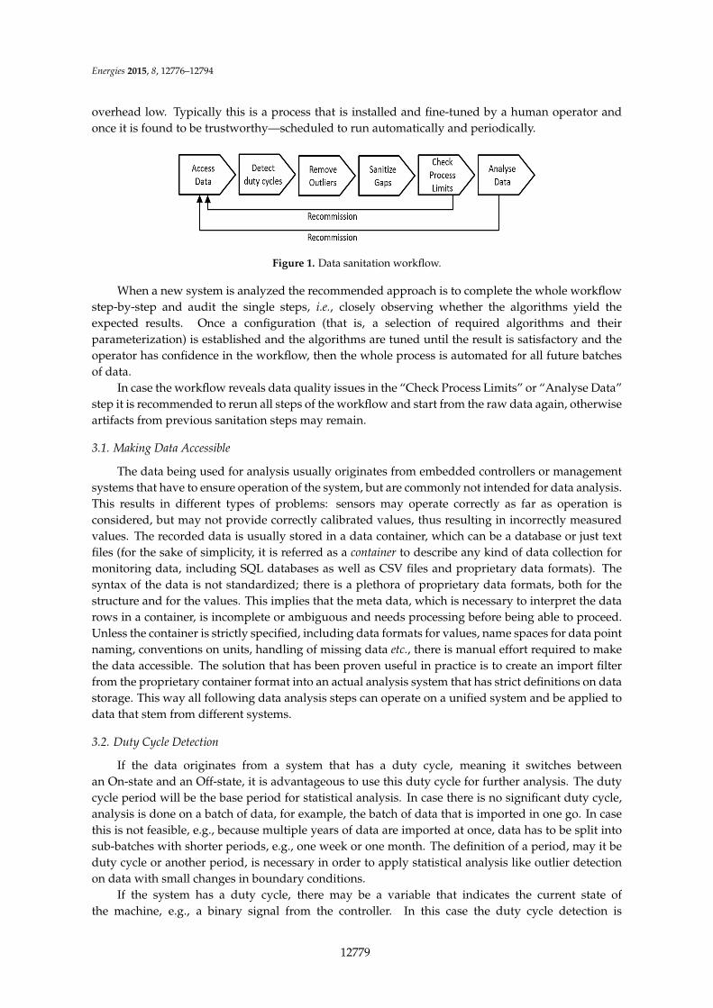
Figure 1. Data sanitation workflow.

When a new system is analyzed the recommended approach is to complete the whole

workflow step‐by‐step and audit the single steps, i.e., closely observing whether the algorithms yield

the expected results. Once a configuration (that is, a selection of required algorithms and their

parameterization) is established and the algorithms are tuned until the result is satisfactory and the

operator has confidence in the workflow, then the whole process is automated for all future batches

of data.

In case the workflow reveals data quality issues in the “Check Process Limits” or “Analyse Data”

step it is recommended to rerun all steps of the workflow and start from the raw data again,

otherwise artifacts from previous sanitation steps may remain.

3.1. Making Data Accessible

The data being used for analysis usually originates from embedded controllers or management

systems that have to ensure operation of the system, but are commonly not intended for data

analysis. This results in different types of problems: sensors may operate correctly as far as

operation is considered, but may not provide correctly calibrated values, thus resulting in

incorrectly measured values. The recorded data is usually stored in a data container, which can be a

database or just text files (for the sake of simplicity, it is referred as a container to describe any kind

of data collection for monitoring data, including SQL databases as well as CSV files and proprietary

data formats). The syntax of the data is not standardized; there is a plethora of proprietary data

formats, both for the structure and for the values. This implies that the meta data, which is

necessary to interpret the data rows in a container, is incomplete or ambiguous and needs

processing before being able to proceed. Unless the container is strictly specified, including data

formats for values, name spaces for data point naming, conventions on units, handling of missing

data etc., there is manual effort required to make the data accessible. The solution that has been

proven useful in practice is to create an import filter from the proprietary container format into an

actual analysis system that has strict definitions on data storage. This way all following data analysis

steps can operate on a unified system and be applied to data that stem from different systems.

3.2. Duty Cycle Detection

If the data originates from a system that has a duty cycle, meaning it switches between an

On‐state and an Off‐state, it is advantageous to use this duty cycle for further analysis. The duty

cycle period will be the base period for statistical analysis. In case there is no significant duty cycle,

analysis is done on a batch of data, for example, the batch of data that is imported in one go. In case

this is not feasible, e.g., because multiple years of data are imported at once, data has to be split into

sub‐batches with shorter periods, e.g., one week or one month. The definition of a period, may it be

duty cycle or another period, is necessary in order to apply statistical analysis like outlier detection

on data with small changes in boundary conditions.

If the system has a duty cycle, there may be a variable that indicates the current state of the

machine, e.g., a binary signal from the controller. In this case the duty cycle detection is straight

forward by using this variable. Otherwise the duty cycle has to be derived from other process

variables such as temperature levels or mass flows. For this detection a robust algorithm is required

that can automatically process the data batches. The k‐means clustering algorithm has been

Figure 1. Data sanitation workflow.

When a new system is analyzed the recommended approach is to complete the whole workflowstep-by-step and audit the single steps, i.e., closely observing whether the algorithms yield theexpected results. Once a configuration (that is, a selection of required algorithms and theirparameterization) is established and the algorithms are tuned until the result is satisfactory and theoperator has confidence in the workflow, then the whole process is automated for all future batchesof data.

In case the workflow reveals data quality issues in the “Check Process Limits” or “Analyse Data”step it is recommended to rerun all steps of the workflow and start from the raw data again, otherwiseartifacts from previous sanitation steps may remain.

3.1. Making Data Accessible

The data being used for analysis usually originates from embedded controllers or managementsystems that have to ensure operation of the system, but are commonly not intended for data analysis.This results in different types of problems: sensors may operate correctly as far as operation isconsidered, but may not provide correctly calibrated values, thus resulting in incorrectly measuredvalues. The recorded data is usually stored in a data container, which can be a database or just textfiles (for the sake of simplicity, it is referred as a container to describe any kind of data collection formonitoring data, including SQL databases as well as CSV files and proprietary data formats). Thesyntax of the data is not standardized; there is a plethora of proprietary data formats, both for thestructure and for the values. This implies that the meta data, which is necessary to interpret the datarows in a container, is incomplete or ambiguous and needs processing before being able to proceed.Unless the container is strictly specified, including data formats for values, name spaces for data pointnaming, conventions on units, handling of missing data etc., there is manual effort required to makethe data accessible. The solution that has been proven useful in practice is to create an import filterfrom the proprietary container format into an actual analysis system that has strict definitions on datastorage. This way all following data analysis steps can operate on a unified system and be applied todata that stem from different systems.

3.2. Duty Cycle Detection

If the data originates from a system that has a duty cycle, meaning it switches betweenan On-state and an Off-state, it is advantageous to use this duty cycle for further analysis. The dutycycle period will be the base period for statistical analysis. In case there is no significant duty cycle,analysis is done on a batch of data, for example, the batch of data that is imported in one go. In casethis is not feasible, e.g., because multiple years of data are imported at once, data has to be split intosub-batches with shorter periods, e.g., one week or one month. The definition of a period, may it beduty cycle or another period, is necessary in order to apply statistical analysis like outlier detectionon data with small changes in boundary conditions.

If the system has a duty cycle, there may be a variable that indicates the current state ofthe machine, e.g., a binary signal from the controller. In this case the duty cycle detection is

12779

Energies 2015, 8, 12776–12794

straight forward by using this variable. Otherwise the duty cycle has to be derived from otherprocess variables such as temperature levels or mass flows. For this detection a robust algorithmis required that can automatically process the data batches. The k-means clustering algorithm hasbeen successfully used for duty cycle detection [20,21]. k-means is a method of finding clusters indata based on the squared error criteria [22]. The k-means algorithm finds the k-partitions in sucha way that in each partition the squared error between the mean (µk) of a cluster and the points inthe cluster is minimized. Let A = {ai}, i = 1, . . . ,n be the set of n patterns and that is required to beclustered into a set of K clusters, C = {Ck, k = 1, . . . ,K}. Let µk be the mean of cluster Ck. The squarederror between µk and the points in cluster Ck is defined as:

J pCkq “

nÿ

xi P Ck

‖ xi ´ µk ‖2 (1)

The goal of k-means is to minimize the sum of the squared error over all K clusters:

J pCq “K

ÿ

k“1

nÿ

xi P Ck

‖ xi ´ µk ‖2 (2)

The main steps of k-means algorithm are as follows:

1) Generate the initial partitions of K clusters.2) Assign the cluster to each pattern on the basis of its closest cluster center.3) Calculate the new cluster centers.4) Repeat Steps 2 and 3 until all the patterns are assigned the cluster.

The k-means algorithm detects the On/Off state of a system; a duty cycle is then defined to be thesequence of one On-state followed by one Off-state. The benefit of k-means is that the algorithm workson scalar values and does not need predefined process limits. The only configuration effort requiredis to tag the detected states as On-state or Off-state, for example, the high temperature cluster reflectsthe On-state, the low temperature cluster is the Off-state. The state and duty cycle detection is appliedto the demo system in Section 5.3.

3.3. Removal of Outliers

Data that originates from the operation of a system typically contains samples that are notwithin the process limits (e.g., the allowed temperature range or the maximum possible mass flowin a process), but that do not necessarily indicate faulty operation of the system. In case the outliersare singletons or a limited amount of consecutive samples, it is reasonable to sanitize the data byremoving the outliers and replacing them by physically plausible data samples. This task can be doneby a human operator who requires only limited knowledge on the underlying physical processes(typically knowing the process limits is sufficient).

However, the challenge is to automate this process so that no human intervention is required.Algorithms from the domain of machine learning can be applied to solve this issue by clustering dataand identifying the clusters which denote outliers. Clustering shall again be executed automaticallywith a minimum configuration effort, meaning that it shall be possible to detect outliers, even ifinformation like process limits are missing.

The outlier detection process described here uses z-scores, see e.g., [23]. It operates automaticallyand does not require configuration. However, the performance of the outlier detection benefits fromthe duty cycle detection: z-score considers the mean and standard deviation of the whole data fornormalization; this way outliers are better distinguishable from normal behavior, thus improving theclustering algorithm that identifies the outliers.

12780

Energies 2015, 8, 12776–12794

Furthermore, systems with a duty cycle typically have different operation ranges during On-and Off-state. If the z-score would consider the whole duty cycle as one, there is a higher chance thatit neglects or considers the correct data points as erroneous data points. To overcome this problem,this research suggests to derive the z-score separately for On-state and Off-state as following wherez-scoreCycle is the z-score for each state in a duty cycle, X is the value of the sensor, µCycle is thepopulation mean of each state in the cycle, and σCycle is the standard deviation of each state inthe cycle:

z´ scoreCycle “ pX ´ µCycleq{σCycle (3)

Expectation Maximization (EM) is a method for finding the maximum likelihood estimates ofthe data distribution when data is unknown or hidden. The EM clustering algorithm uses the finiteGaussian mixtures model, then tries to estimate a set of parameters until the anticipated convergencevalue is achieved. Now the mixture has K probability distributions in which each distributionrepresents one cluster. For each instance the class membership is assigned with the maximumprobability. The working of EM algorithm can be defined as follows [24]:

1) Start with guessing the initial parameters: mean and standard deviation (in case the normaldistribution model is being used).

2) Now enhance the parameters with E (Expectation) and M (Maximization) steps iteratively. Inthe E step, the membership probability for each instance on the bases of the initial parametersis calculated. Whereas in the M step the parameters are recalculated on the base of newmembership likelihoods.

3) Allocate each instance of the data to the cluster with which it has the highest likelihood probability.

In order to enable the EM clustering algorithm to decide the number of clusters automatically,the cross validation method is used [25,26]. The cross validation is done using the following steps:

1) Initially the number of clusters is set to 1.2) The training set is randomly divided into 10 folds.3) The Expectation Maximization (EM) is applied to each fold using cross validation.4) The average log likelihood of the 10 results is calculated; if the log likelihood is increased then the

number of clusters is increased by 1 and it goes back to Step 2 again.

3.4. Sanitation of Gaps

Gaps in the recording of data occur in daily operation e.g., due to communication glitches orother interruptions in monitoring. Also the previously presented removal of outliers (Section 3.3)causes gaps in the data that need to be repaired. Two types of gaps can be distinguished: short gapscan be fixed by interpolation between the two adjacent samples. Sanitation of longer gaps requiresa closer inspection of the data at hand and shall therefore be done in the analysis-step with supportof a regression analysis as described in Section 5.6.1.

The definition of how long a gap shall be in order to be fixed by interpolation depends onthe dynamics of the underlying process. For highly dynamic processes the gap period should beshort, otherwise data quality decreases. A “hands-on” approach is to rely on the assumption thatthe monitoring system has a sample rate that is consistent with the dynamics of the system. Electricenergy meters, for example typically take a sample every 15 min, since this is adequate for observingthe load profile. The same applies for slow thermal processes like heating and cooling in buildings.Under the assumption that the maximum relevant frequency in a process is correlated with the samplerate it is sensitive to define the measure the maximum length of an automatically sanitizable gap.In the daily work with monitoring data of thermal systems a maximum gap length of ten samplesproved feasible. This will, however, still requires further analysis, depending on the expected resultsthat the monitoring data shall yield.

12781

Energies 2015, 8, 12776–12794

3.5. Checking Data against Process Limits

For selected data points it is reasonable to define process limits, such as e.g., a valid temperaturerange for inlet and outlet temperatures or maximum power consumption of an electric motor. Whenintroducing knowledge about the process, a minimal configuration effort is introduced, requiringa level of information that is typically found on the data sheet of a component. When applyingthe data sanitation workflow it may be feasible to configure process limits for selected data points,given that the benefits outweigh the effort and that additional trust in the data can be gained. Threeexamples from real world experience shall illustrate this:

‚ Due to maintenance the configuration may change and thus the semantic link between controllerand monitoring system may be broken, which can result in data rows being stored at wrong datapoints. Especially a local buffer that is periodically transferred to a central data collection is proneto such errors. Due to software updates the assignment between sensor identification and exporteddata rows may be reassigned, yielding to incorrect configuration.

‚ Electric and thermal meters often have preconfigured conversion factors that are used to convertthe numeric meter value into a valid physical unit like kWh. If this conversion factor is not properlyset during commissioning or if it changes, e.g., due to replacement of the meter, the monitoring ofhistoric values is broken.

‚ Unit conversions, e.g., from Kelvin to Celsius, also break the semantic link between numeric valueand physical parameter, if they are not properly regarded.

All of the above issues can be identified by introducing process limits: incorrectly assigned datapoints will violate the upper or lower limit; for energy meters a maximum energy per period can beset—and checked by deriving the power from the recorded energy consumption; unit conversionsare also detected, since the numeric values will likely not fit in the process limit. Section 5.5 showsan application of process limits by means of histograms as this is a convenient method to visualizethe plausibility of data by separating valid from invalid data.

3.6. Analysis of Data

Under the assumption that data is free of outliers and is within process limits, the data qualitycan be further increased by introducing additional aspects of the process. Energy components inHVAC systems often have a clear system boundary that can be used to analyze the energy balance,mass balance or—derived from these balances—the power balance or mass flow balance. Energy balancecan be examined when the main parameters are measured and stored– for example heat meters inthe high temperature circuit, low temperature circuit and cooling tower circuit (as shown in thedemonstration system in in Section 5.1). Data can then be validated based on the assumption thatthe energy in a system remains constant, resulting in the sum of all thermal energy flows to be zero.While this will not hold for strict mathematical equality, especially because thermal losses are notmeasured and thermal capacities differ, it still gives a good indicator on the plausibility of the data.In a similar way the data quality can be improved by analyzing the mass flows in a system to indicatepossible issues in sensory equipment, calibration, commissioning or data transfer.

4. Architectural Aspects of the Data Storage and Analysis System

The process described in the previous section requires a set of methods and data views thatare summarized in Table 1. It also requires a data storage system that has certain properties; theproperties which are necessary for the scope of this paper are described in this section.

4.1. Database System

As described previously, monitoring of operation data in the field likely contains some incorrectvalues or values outside the specified range of operation. In the first steps of data collection all data

12782

Energies 2015, 8, 12776–12794

has to be treated with caution, since it is not clear which data is trustable and which is not. Thereforeraw data is never deleted or overwritten since the sanitation and correction algorithms may be rerunwith improved configuration parameters. To achieve this, a layer model for data storage is used inthis work (Figure 2). The data row Raw is populated during the import of a batch of raw data togetherwith a timestamp of the sampling time (for illustration purposes, only hour and minute are shown inFigure 2). In this example a sample is taken every five minutes. Each sample has a tag faulty (F) that isstored in the database. The outlier removal (Section 3.3), the check against process limits (Section 3.5)and the analysis by a domain expert (Section 3.6) may mark data samples as faulty (F) indicating thatthese samples are not reliable. In the example in Figure 2, values between 0 and 60 are valid, resultingin the samples at 20:00 and 30:00 being marked as faulty. The figure also shows that there are nosamples available at 00:05, 35:00 and 40:00.


8

samples as faulty (F) indicating that these samples are not reliable. In the example in Figure 2,

values between 0 and 60 are valid, resulting in the samples at 20:00 and 30:00 being marked as

faulty. The figure also shows that there are no samples available at 00:05, 35:00 and 40:00.

Figure 2. Raw data with faulty and missing data.

Data sanitation as described in Section 3.4 or for lager gaps in Section 5.6.1, operates on

missing and faulty data and sanitizes the data row in order to get a consistent and plausible time

series. The results are stored in a new data row in the database as shown in Figure 3. For sanitized

samples the flag synthetic (S) is set and a new data row Clean is filled with raw and synthetic data.

The missing or faulty data are filled using linear interpolation; note that the Clean data row contains

more samples than the Raw data row, since the missing samples at 00:05, 35:00 and 40:00 have

been inserted.

Figure 3. The Clean data row containing raw and synthetic data after the sanitation process.

4.2. Data Views

Stored data can be accessed in different views. Many legacy systems can operate with data

rows only on the base of time stamp and value. In case it is necessary to examine raw data with

such a system, the additional meta‐information on faulty and missing data cannot be transported.

Therefore a view as shown in Figure 4 is used: all missing and faulty data are filled with zeroes,

allowing the legacy system to operate with equidistant values free of gaps. Note that the Legacy data

row is only a view that is not stored in the database, but is created upon request.

Figure 4. A view on the data for legacy system setting all faulty and missing data to zero.

Another important method of supporting the user is to provide aligned data series. The data

samples may be not be exactly equidistant, but rather may have jitter around the intended sample


Data sanitation as described in Section 3.4 or for lager gaps in Section 5.6.1, operates on missingand faulty data and sanitizes the data row in order to get a consistent and plausible time series. Theresults are stored in a new data row in the database as shown in Figure 3. For sanitized samples theflag synthetic (S) is set and a new data row Clean is filled with raw and synthetic data. The missing orfaulty data are filled using linear interpolation; note that the Clean data row contains more samplesthan the Raw data row, since the missing samples at 00:05, 35:00 and 40:00 have been inserted.


8











been inserted.


4.2. Data Views











4.2. Data Views

Stored data can be accessed in different views. Many legacy systems can operate with datarows only on the base of time stamp and value. In case it is necessary to examine raw data withsuch a system, the additional meta-information on faulty and missing data cannot be transported.Therefore a view as shown in Figure 4 is used: all missing and faulty data are filled with zeroes,allowing the legacy system to operate with equidistant values free of gaps. Note that the Legacy datarow is only a view that is not stored in the database, but is created upon request.


8











been inserted.


4.2. Data Views











12783

Energies 2015, 8, 12776–12794

Another important method of supporting the user is to provide aligned data series. The datasamples may be not be exactly equidistant, but rather may have jitter around the intended sampleinterval. In the example above, the time stamps may vary a few seconds as different sensors may besampled too early or too late. For small jitter the Snap-to-grid view can be used. This view returns timestamps that are exactly equidistant and uses the closest sample to this timestamp. The underlyingalgorithm is executed only upon request and does not store the data in the database. It looks for a datasample within the sample interval and modifies its time stamp. Assuming that the sample intervalhas a sufficient resolution, the sample can just be taken as is. In case the sample interval changes(like in the following Sample-Interval-Variation view) the sample has to be interpolated between theneighboring samples in order to keep the error low.

Once a database is used that allows to separate stored data from viewed data, it is possibleto query data with a sample interval different from the raw data sample interval. This becomeshandy when e.g., temperatures with 5-min intervals and meter readings with 15-min intervals shallbe compared in the same graph. The Sample-Interval-Variation view can deliver data with a specifiedsample interval, which may be shorter than the raw data interval in which case additional samples areinterpolated or longer, meaning that several samples are averaged. Again the algorithm for varyingthe sample interval is executed on demand.

4.3. Overview of Methods and Views

The workflow shown in Figure 1 depends on a combination of methods and views that have tosupport human users who examine the data. They also need to be automatable in order to integrateperiodic batches of newly imported data into the existing database. Table 1 lists the sequence ofmethods and views as they can be applied to raw data.

5. Demonstration System: Adsorption Chiller

This section applies the data sanitation workflow to an energy system that provides integratedmonitoring of its main operation parameters. By analyzing the available data with regard to dataquality, the workflow is validated and proven to be feasible. The execution of the workflow was setup such that the data related issues such as data access and outlier detection were addressed by ITexperts. The validation steps that require limited domain knowledge were also done by IT expertswith minor feedback from energy domain experts. After the workflow was executed the data waspresented to energy experts and their feedback was provided: the data quality has been significantlyincreased, allowing discussions on how to further improve the design and the operation of the system.As a result the controller software has been updated to improve operation.

5.1. System Setup

The data used for this research has been taken from a water/silica gel based adsorption chiller,which is manufactured by the company Pink (Langenwang, Styria, Austria). The system uses hotwater that is produced by solar power to produce cold water. Applications are, for example, coolingof meeting rooms and big event facilities, but also cooling facilities for food products. The designof the system is shown in Figure 5, showing the Low Temperature (LT), Medium Temperature (MT)and High Temperature (HT) cycles along with the installed sensors that are used for analysis. For thescope of this paper a total of 15 data points are used (Table 2).

The measured monitoring data is generated by the embedded controller of the chiller systems;it can be accessed via HTML requests using the built-in web server, which issues an XML documentcontaining the current data. The data from the controller is recorded and stored in a monitoringand analysis system called OpenJEVis [27]. OpenJEVis is an open source system for monitoringand analyzing energy data, which provides data storage and visualization features. It also providesthe meta-data structures for tagging data as faulty and allows for different views on the data. Foraccessing the data of the demonstration system, the flexible import features were used: a driver was

12784

Energies 2015, 8, 12776–12794

written in Java to periodically poll the chiller controller. During storing, the data is not processed orvalidated; this is done later within the OpenJEVis system.


10

Figure 5. Adsorption chiller system configuration.

Table 1. Parameters Description.

Sensors Description

HT_Elec Electricity consumption meter reading at high temperature cycle

MT_Elec Electricity consumption meter reading at medium temperature cycle

LT_Elec Electricity consumption meter reading at low temperature cycle

HT_Flow Flow of water readings in high temperature cycle

MT_Flow Flow of water readings in medium temperature cycle

LT_Flow Flow of water readings in low temperature cycle

T_HTre Temperature reading at high temperature cycle on return side

T_HTsu Temperature reading at high temperature cycle on supply side

T_MTre Temperature reading at medium temperature cycle on return side

T_MTsu Temperature reading at medium temperature cycle on supply side

T_LTre Temperature reading at low temperature cycle on return side

T_LTsu Temperature reading at low temperature cycle on supply side

QHT Energy consumption reading at high temperature cycle

QMT Energy consumption reading at medium temperature cycle

QLT Energy consumption reading at low temperature cycle

5.2. Data Availability of Monitoring Data

Availability of monitoring data can be retrieved from the database by finding the gaps in data

recording. In order to give a comprehensive overview of the availability a calendar view was

chosen as shown in Figure 6. It shows the data availability of one chiller system, consisting of

15 data points (the parameters listed in Table 2) from June 2009 to October 2010 with a sampling

interval of 4 min. Data is considered being missing if there is no data sample within a 4 min

interval. The available data samples are counted and a color is assigned depending on the ratio of

actual versus available data samples (in this example at most 15 data samples).

The calendar view has different application in the data sanitation process: it may also be

configured to show the availability of valid data, i.e., data that are not marked as faulty and are

within process limits.

Figure 5. Adsorption chiller system configuration.

Table 2. Parameters Description.

Sensors Description

HT_Elec Electricity consumption meter reading at high temperature cycleMT_Elec Electricity consumption meter reading at medium temperature cycleLT_Elec Electricity consumption meter reading at low temperature cycle

HT_Flow Flow of water readings in high temperature cycleMT_Flow Flow of water readings in medium temperature cycleLT_Flow Flow of water readings in low temperature cycleT_HTre Temperature reading at high temperature cycle on return sideT_HTsu Temperature reading at high temperature cycle on supply sideT_MTre Temperature reading at medium temperature cycle on return sideT_MTsu Temperature reading at medium temperature cycle on supply sideT_LTre Temperature reading at low temperature cycle on return sideT_LTsu Temperature reading at low temperature cycle on supply side

QHT Energy consumption reading at high temperature cycleQMT Energy consumption reading at medium temperature cycleQLT Energy consumption reading at low temperature cycle

5.2. Data Availability of Monitoring Data

Availability of monitoring data can be retrieved from the database by finding the gaps in datarecording. In order to give a comprehensive overview of the availability a calendar view was chosenas shown in Figure 6. It shows the data availability of one chiller system, consisting of 15 data points(the parameters listed in Table 2) from June 2009 to October 2010 with a sampling interval of 4 min.Data is considered being missing if there is no data sample within a 4 min interval. The available datasamples are counted and a color is assigned depending on the ratio of actual versus available datasamples (in this example at most 15 data samples).

12785

Energies 2015, 8, 12776–12794

The calendar view has different application in the data sanitation process: it may also beconfigured to show the availability of valid data, i.e., data that are not marked as faulty and are withinprocess limits.

The calendar view does not require domain knowledge and provides a good overview. It isa starting point for further investigations, since the problematic time periods can be identified easily.In the given example the chiller is only in operation during the cooling season in summer, thusthere is little data expected except for summer. The data gaps, e.g., on 6 September 2010, can beconveniently visualized.


11

The calendar view does not require domain knowledge and provides a good overview. It is a

starting point for further investigations, since the problematic time periods can be identified easily.

In the given example the chiller is only in operation during the cooling season in summer, thus

there is little data expected except for summer. The data gaps, e.g., on 6 September 2010, can be

conveniently visualized.

Figure 6. Calendar view of data availability: two years of operation, one system with 15 data points.

5.3. On/Off State Detection and Duty Cycle Detection

In order to detect the On/Off state and the resulting duty cycle automatically, the k‐means

clustering algorithm is used as explained in Section 3.2. Before using the k‐means clustering, the

data is normalized by using Min‐Max normalization method with values in the range of

0 (minimum) to 1 (maximum). The number of clusters is set to two (On‐state and Off‐state) and the

Euclidean distance is selected for finding the given number of clusters for both levels.

The consecutive On states are considered as one cycle. The same process is repeated for all the

consecutive On/Off states. The k‐means algorithm is applied to monitoring data from the adsorption

chiller in a period of 17 months (June 2009 to October 2010) and derives the state by using the

15 variables discussed in Table 2. The data is clustered automatically, meaning that after running

the k‐means algorithm the detected On/Off state can be stored and used as the base for the next

steps of data analysis.

The detected On/Off states are shown in Figure 7 and demonstrate how the time series data are

now supported by an additional On/Off state time series (the red line in the last graph of Figure 7

shows the On and Off‐state). The dashed rectangle in Figure 7 shows that the rising of high and

medium temperatures together with the decreasing low temperature verifies that the chiller is in

operation and directly matches the detected On‐state variable.

In order to validate the On/Off status by the k‐means algorithm, the k‐means algorithm has

been applied to the five systems having a known On/Off status. Table 3 shows the accuracy rate of

the k‐means applied on the five systems. The average accuracy of the k‐means is around 99%. The

Figure 6. Calendar view of data availability: two years of operation, one system with 15 data points.

5.3. On/Off State Detection and Duty Cycle Detection

In order to detect the On/Off state and the resulting duty cycle automatically, the k-meansclustering algorithm is used as explained in Section 3.2. Before using the k-means clustering, the datais normalized by using Min-Max normalization method with values in the range of 0 (minimum)to 1 (maximum). The number of clusters is set to two (On-state and Off-state) and the Euclideandistance is selected for finding the given number of clusters for both levels. The consecutive On statesare considered as one cycle. The same process is repeated for all the consecutive On/Off states. Thek-means algorithm is applied to monitoring data from the adsorption chiller in a period of 17 months(June 2009 to October 2010) and derives the state by using the 15 variables discussed in Table 2.The data is clustered automatically, meaning that after running the k-means algorithm the detectedOn/Off state can be stored and used as the base for the next steps of data analysis.

The detected On/Off states are shown in Figure 7 and demonstrate how the time series data arenow supported by an additional On/Off state time series (the red line in the last graph of Figure 7shows the On and Off-state). The dashed rectangle in Figure 7 shows that the rising of high andmedium temperatures together with the decreasing low temperature verifies that the chiller is inoperation and directly matches the detected On-state variable.

In order to validate the On/Off status by the k-means algorithm, the k-means algorithm hasbeen applied to the five systems having a known On/Off status. Table 3 shows the accuracy rate ofthe k-means applied on the five systems. The average accuracy of the k-means is around 99%. The

12786

Energies 2015, 8, 12776–12794

k-means algorithm has lower accuracy rate in transient phase of the machine where the machines arejust starting.


12

k‐means algorithm has lower accuracy rate in transient phase of the machine where the machines

are just starting.

Figure 7. Automatically detected On/Off state time series using k‐means clustering algorithm.

Table 3. K‐Means On/Off accuracy.

S. No System Name From To K‐Means On/

Off Accuracy (%)

1 AEE—Gleisdorf (Machine 1) 18 June 2013 9 March 2014 99.94%

2 Behmann‐Egg (Machine 2) 25 June 2013 28 April 2015 99.42%

3 HIZ‐Zeltweg (Machine 3) 24 July 2013 27 April 2015 95.77%

4 Koegerlhof‐Hartmannsdorf (Machine 4) 27 Janurary 2014 27 April 2015 99.92%

5 Privathaus‐Niederoesterreich (Machine 5) 10 March 2013 27 April 2015 99.21%

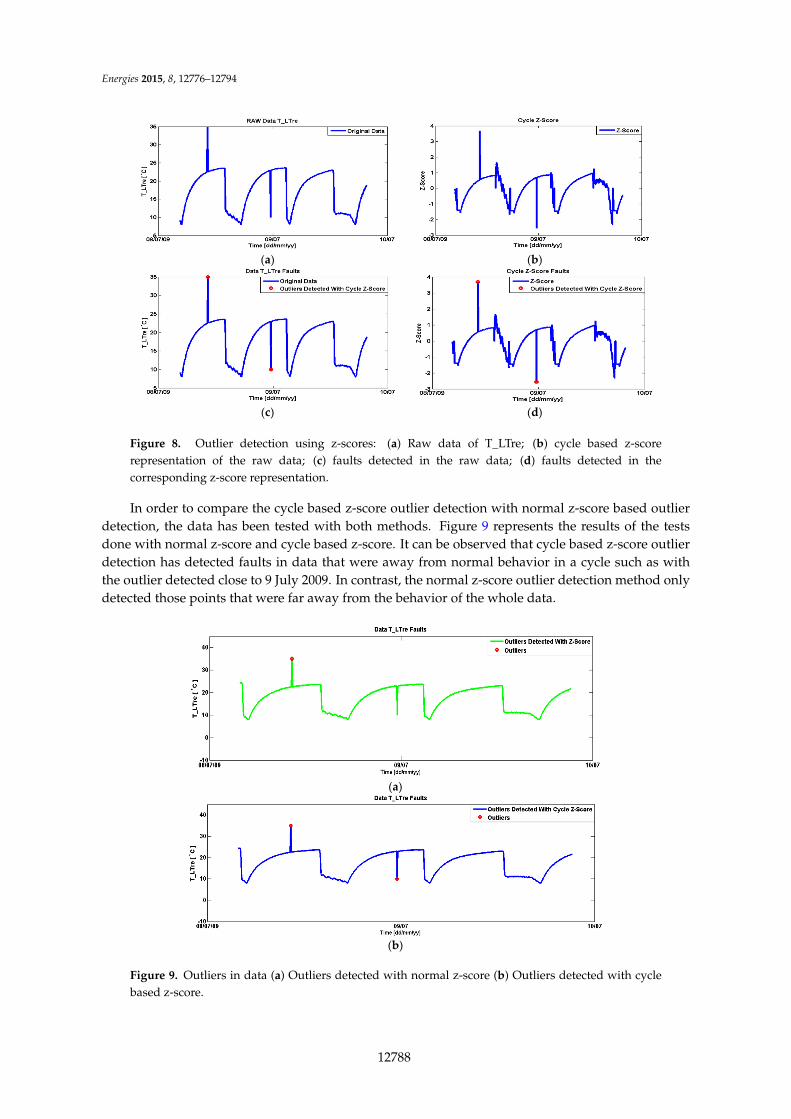
5.4. Outlier Detection Using Z‐Score Normalization

In order to detect outliers in the data the duty cycle based z‐score is applied as described in

Section 3.3. The statistical data for the z‐scores (μ and σ) are derived based on single duty cycles

instead of e.g., a whole day. During the transient phase where the chiller is changing its state from

either On to Off or vice versa, the initial behavior does not exhibit the normal behavior of the cycle.

Therefore the transient phase of 30 min during Off‐state and 4 min of On‐state are not considered

for the mean and standard deviation of the respective cycle. Figure 8 shows the original data

(T_LTre) along with the duty cycle z‐score; the detected outliers using expectation maximization

clustering (EM) algorithm are marked with red circles both in the original data and in the z‐scored

data. These outliers are, however, only single samples and can be restored by simple gap filling as

described in Section 5.6.1. Furthermore, the change of specific On‐state and Off‐state z‐score

parameters allows for better detection of outliers, since the behavior of a process can strongly differ

between two operational states.

Figure 7. Automatically detected On/Off state time series using k-means clustering algorithm.

Table 3. K-Means On/Off accuracy.

S. No System Name From To K-Means On/OffAccuracy (%)

1 AEE—Gleisdorf (Machine 1) 18 June 2013 9 March 2014 99.94%2 Behmann-Egg (Machine 2) 25 June 2013 28 April 2015 99.42%3 HIZ-Zeltweg (Machine 3) 24 July 2013 27 April 2015 95.77%4 Koegerlhof-Hartmannsdorf (Machine 4) 27 Janurary 2014 27 April 2015 99.92%5 Privathaus-Niederoesterreich (Machine 5) 10 March 2013 27 April 2015 99.21%

5.4. Outlier Detection Using Z-Score Normalization

In order to detect outliers in the data the duty cycle based z-score is applied as described inSection 3.3. The statistical data for the z-scores (µ and σ) are derived based on single duty cyclesinstead of e.g., a whole day. During the transient phase where the chiller is changing its state fromeither On to Off or vice versa, the initial behavior does not exhibit the normal behavior of the cycle.Therefore the transient phase of 30 min during Off-state and 4 min of On-state are not considered forthe mean and standard deviation of the respective cycle. Figure 8 shows the original data (T_LTre)along with the duty cycle z-score; the detected outliers using expectation maximization clustering(EM) algorithm are marked with red circles both in the original data and in the z-scored data. Theseoutliers are, however, only single samples and can be restored by simple gap filling as described inSection 5.6.1. Furthermore, the change of specific On-state and Off-state z-score parameters allowsfor better detection of outliers, since the behavior of a process can strongly differ between twooperational states.

12787

Energies 2015, 8, 12776–12794Energies 2015, 8, page–page

13

(a) (b)

(c) (d)

Figure 8. Outlier detection using z‐scores: (a) Raw data of T_LTre; (b) cycle based z‐score

representation of the raw data; (c) faults detected in the raw data; (d) faults detected in the

corresponding z‐score representation.

In order to compare the cycle based z‐score outlier detection with normal z‐score based outlier

detection, the data has been tested with both methods. Figure 9 represents the results of the tests

done with normal z‐score and cycle based z‐score. It can be observed that cycle based z‐score outlier

detection has detected faults in data that were away from normal behavior in a cycle such as with

the outlier detected close to 9 July 2009. In contrast, the normal z‐score outlier detection method

only detected those points that were far away from the behavior of the whole data.

(a)

(b)

Figure 9. Outliers in data (a) Outliers detected with normal z‐score (b) Outliers detected with cycle

based z‐score.

Figure 8. Outlier detection using z-scores: (a) Raw data of T_LTre; (b) cycle based z-scorerepresentation of the raw data; (c) faults detected in the raw data; (d) faults detected in thecorresponding z-score representation.

In order to compare the cycle based z-score outlier detection with normal z-score based outlierdetection, the data has been tested with both methods. Figure 9 represents the results of the testsdone with normal z-score and cycle based z-score. It can be observed that cycle based z-score outlierdetection has detected faults in data that were away from normal behavior in a cycle such as withthe outlier detected close to 9 July 2009. In contrast, the normal z-score outlier detection method onlydetected those points that were far away from the behavior of the whole data.


13

(a) (b)

(c) (d)

Figure 8. Outlier detection using z‐scores: (a) Raw data of T_LTre; (b) cycle based z‐score

representation of the raw data; (c) faults detected in the raw data; (d) faults detected in the

corresponding z‐score representation.

In order to compare the cycle based z‐score outlier detection with normal z‐score based outlier

detection, the data has been tested with both methods. Figure 9 represents the results of the tests

done with normal z‐score and cycle based z‐score. It can be observed that cycle based z‐score outlier

detection has detected faults in data that were away from normal behavior in a cycle such as with

the outlier detected close to 9 July 2009. In contrast, the normal z‐score outlier detection method

only detected those points that were far away from the behavior of the whole data.

(a)

(b)

Figure 9. Outliers in data (a) Outliers detected with normal z‐score (b) Outliers detected with cycle

based z‐score. Figure 9. Outliers in data (a) Outliers detected with normal z-score (b) Outliers detected with cyclebased z-score.

12788

Energies 2015, 8, 12776–12794

5.5. Visualization of Process Limits

The check against process limits as described in Section 3.5 can be used to visualize statisticalinformation about the data distribution. In combination with duty cycle detection this providesa swift way of visually checking data plausibility: by visualizing only data from the On-state of thesystem, the number of process limit violations is strongly reduced, thus giving insight into the realoperation of the system. If data from the Off-cycle was also regarded, there would be a large amountof (irrelevant) violations. Figures 10 and 11 show two system temperatures in specifically adaptedhistograms: the data within the process limits are equally divided into ten bins; on the upper andlower boundary there is one additional process limits violation bin that contains all remaining outliers(for better visualization these two bins are drawn with red bars, see Figure 10). Figure 11 containsdata with no outliers, which is indicated by the violation bins to have +8 as the upper boundary and´8 as the lower boundary. This allows to check that there is not a single violation in this data.


14


The check against process limits as described in Section 3.5 can be used to visualize statistical

information about the data distribution. In combination with duty cycle detection this provides a

swift way of visually checking data plausibility: by visualizing only data from the On‐state of the

system, the number of process limit violations is strongly reduced, thus giving insight into the real

operation of the system. If data from the Off‐cycle was also regarded, there would be a large

amount of (irrelevant) violations. Figures 10 and 11 show two system temperatures in specifically

adapted histograms: the data within the process limits are equally divided into ten bins; on the

upper and lower boundary there is one additional process limits violation bin that contains all

remaining outliers (for better visualization these two bins are drawn with red bars, see Figure 10).

Figure 11 contains data with no outliers, which is indicated by the violation bins to have +∞ as the

upper boundary and −∞ as the lower boundary. This allows to check that there is not a single

violation in this data.

Figure 10. Histogram of the supply temperature in the high temperature cycle showing only the

temperatures while the system is on. The data contains outliers.

Figure 11. Histogram of the return temperature in the low temperature cycle showing only the

temperatures while the system is on, showing no outliers (violation bins on the left and right

are empty).

Figure 10. Histogram of the supply temperature in the high temperature cycle showing only thetemperatures while the system is on. The data contains outliers.


14


The check against process limits as described in Section 3.5 can be used to visualize statistical

information about the data distribution. In combination with duty cycle detection this provides a

swift way of visually checking data plausibility: by visualizing only data from the On‐state of the

system, the number of process limit violations is strongly reduced, thus giving insight into the real

operation of the system. If data from the Off‐cycle was also regarded, there would be a large

amount of (irrelevant) violations. Figures 10 and 11 show two system temperatures in specifically

adapted histograms: the data within the process limits are equally divided into ten bins; on the

upper and lower boundary there is one additional process limits violation bin that contains all

remaining outliers (for better visualization these two bins are drawn with red bars, see Figure 10).

Figure 11 contains data with no outliers, which is indicated by the violation bins to have +∞ as the

upper boundary and −∞ as the lower boundary. This allows to check that there is not a single

violation in this data.

Figure 10. Histogram of the supply temperature in the high temperature cycle showing only the

temperatures while the system is on. The data contains outliers.

Figure 11. Histogram of the return temperature in the low temperature cycle showing only the

temperatures while the system is on, showing no outliers (violation bins on the left and right

are empty).

Figure 11. Histogram of the return temperature in the low temperature cycle showing only thetemperatures while the system is on, showing no outliers (violation bins on the left and rightare empty).

12789

Energies 2015, 8, 12776–12794

5.6. Analysis

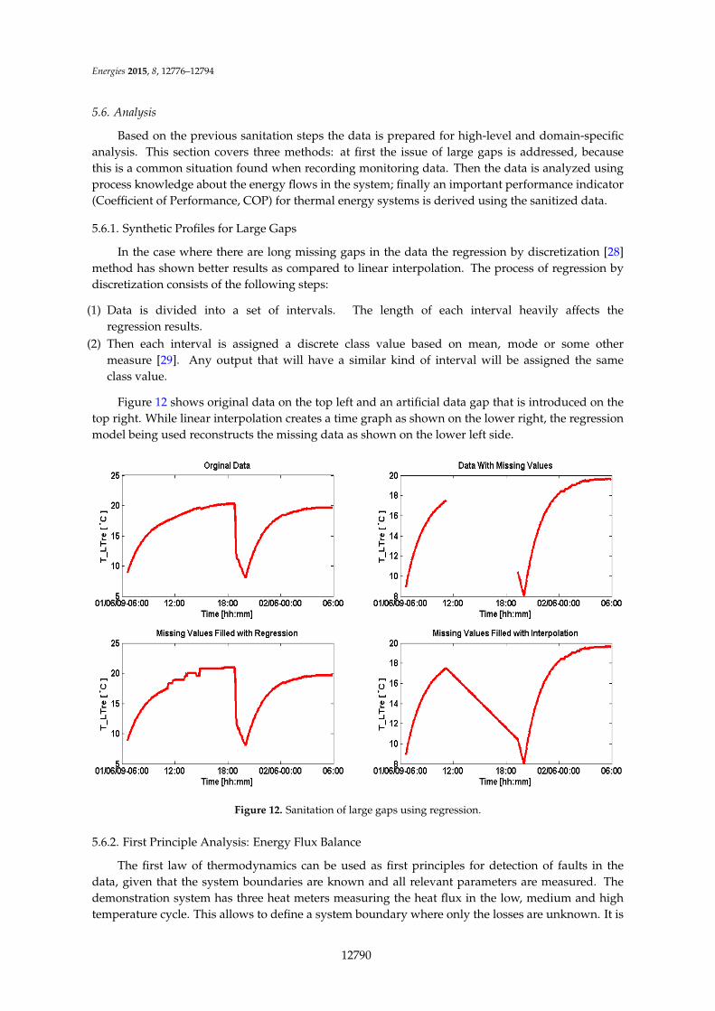
Based on the previous sanitation steps the data is prepared for high-level and domain-specificanalysis. This section covers three methods: at first the issue of large gaps is addressed, becausethis is a common situation found when recording monitoring data. Then the data is analyzed usingprocess knowledge about the energy flows in the system; finally an important performance indicator(Coefficient of Performance, COP) for thermal energy systems is derived using the sanitized data.

5.6.1. Synthetic Profiles for Large Gaps

In the case where there are long missing gaps in the data the regression by discretization [28]method has shown better results as compared to linear interpolation. The process of regression bydiscretization consists of the following steps:

(1) Data is divided into a set of intervals. The length of each interval heavily affects theregression results.

(2) Then each interval is assigned a discrete class value based on mean, mode or some othermeasure [29]. Any output that will have a similar kind of interval will be assigned the sameclass value.

Figure 12 shows original data on the top left and an artificial data gap that is introduced on thetop right. While linear interpolation creates a time graph as shown on the lower right, the regressionmodel being used reconstructs the missing data as shown on the lower left side.


15

5.6. Analysis

Based on the previous sanitation steps the data is prepared for high‐level and domain‐specific

analysis. This section covers three methods: at first the issue of large gaps is addressed, because this

is a common situation found when recording monitoring data. Then the data is analyzed using

process knowledge about the energy flows in the system; finally an important performance

indicator (Coefficient of Performance, COP) for thermal energy systems is derived using the

sanitized data.

5.6.1. Synthetic Profiles for Large Gaps

In the case where there are long missing gaps in the data the regression by discretization [28]

method has shown better results as compared to linear interpolation. The process of regression by

discretization consists of the following steps:

(1) Data is divided into a set of intervals. The length of each interval heavily affects the

regression results.

(2) Then each interval is assigned a discrete class value based on mean, mode or some other

measure [29]. Any output that will have a similar kind of interval will be assigned the same

class value.

Figure 12 shows original data on the top left and an artificial data gap that is introduced on the

top right. While linear interpolation creates a time graph as shown on the lower right, the

regression model being used reconstructs the missing data as shown on the lower left side.

Figure 12. Sanitation of large gaps using regression.

5.6.2. First Principle Analysis: Energy Flux Balance

The first law of thermodynamics can be used as first principles for detection of faults in the

data, given that the system boundaries are known and all relevant parameters are measured.

The demonstration system has three heat meters measuring the heat flux in the low, medium and

high temperature cycle. This allows to define a system boundary where only the losses are

unknown. It is required that the energy that flows into the system should be equal to the energy

that flows out of the system or is stored in the system:

Figure 12. Sanitation of large gaps using regression.

5.6.2. First Principle Analysis: Energy Flux Balance

The first law of thermodynamics can be used as first principles for detection of faults in thedata, given that the system boundaries are known and all relevant parameters are measured. Thedemonstration system has three heat meters measuring the heat flux in the low, medium and hightemperature cycle. This allows to define a system boundary where only the losses are unknown. It is

12790

Energies 2015, 8, 12776–12794

required that the energy that flows into the system should be equal to the energy that flows out of thesystem or is stored in the system:

QLT `QHT ´QMT ` ∆E “ 0 (4)

Therefore:∆E “ ´QLT ˘QHT ˘QMT (5)

Here ∆E represents the combination of losses and changes in the stored energy. Since the chillerdoes not have a significant thermal capacity, the assumption to verify is that ∆E should be close to 0.Figure 13 shows ∆E for eight duty cycles of the adsorption chiller. The values have high dynamicswhen deriving the energy balance on a sample-by-sample base (blue graph). This is expectable dueto the various delays in thermal dissipation and mass flows. When looking at the average over a dutycycle (red graph) the energy balance ranges from ´0.2 kW to 0.2 kW, which is an acceptable range. Inconclusion, the measured data is therefore resilient, the energy balance is plausible and the meteringdata can be used for further analysis. The automated detection of the duty cycle contributes to thisanalysis, since the data in Off-state are commonly not relevant for energy balance analysis.


16

Δ 0 (4)

Therefore:

Δ (5)

Here Δ represents the combination of losses and changes in the stored energy. Since the

chiller does not have a significant thermal capacity, the assumption to verify is that Δ should be

close to 0. Figure 13 shows Δ for eight duty cycles of the adsorption chiller. The values have high

dynamics when deriving the energy balance on a sample‐by‐sample base (blue graph). This is

expectable due to the various delays in thermal dissipation and mass flows. When looking at the

average over a duty cycle (red graph) the energy balance ranges from −0.2 kW to 0.2 kW, which is

an acceptable range. In conclusion, the measured data is therefore resilient, the energy balance is

plausible and the metering data can be used for further analysis. The automated detection of the

duty cycle contributes to this analysis, since the data in Off‐state are commonly not relevant for

energy balance analysis.

Figure 13. Energy flux balance in an adsorption chiller.

5.6.3. Thermal Coefficient of Performance (COPtherm) Calculation

The thermal coefficient of performance (COPtherm) is another analysis method to improve data

quality and to identify faults. The COPtherm of an adsorption chiller has to be in a range between 0 and 1,

a COPtherm outside this range is physically not possible in steady state and therefore is an indicator

for low data quality. The COPtherm is derived using:

Figure 14 shows the thermal COP derived on a sample‐by‐sample base (blue graph) and

averaged over the On‐state of a duty cycle (red graph). Similar to the energy flux balance in the

previous section the average value gives a good indication that the data is plausible.

Figure 15 shows the average COP of cycles for one cooling season. The lower COP ranging

from 0 to 0.1 are cycles with short operational times. The average COP shows that for most cycles

the system performed in the range from 0.3 to 0.6, indicating good performance.

Figure 13. Energy flux balance in an adsorption chiller.

5.6.3. Thermal Coefficient of Performance (COPtherm) Calculation

The thermal coefficient of performance (COPtherm) is another analysis method to improve dataquality and to identify faults. The COPtherm of an adsorption chiller has to be in a range between 0 and1, a COPtherm outside this range is physically not possible in steady state and therefore is an indicatorfor low data quality. The COPtherm is derived using:

COPtherm “QLT

QHT

Figure 14 shows the thermal COP derived on a sample-by-sample base (blue graph) andaveraged over the On-state of a duty cycle (red graph). Similar to the energy flux balance in theprevious section the average value gives a good indication that the data is plausible.

12791

Energies 2015, 8, 12776–12794

Figure 15 shows the average COP of cycles for one cooling season. The lower COP ranging from0 to 0.1 are cycles with short operational times. The average COP shows that for most cycles thesystem performed in the range from 0.3 to 0.6, indicating good performance.Energies 2015, 8, page–page

17

Figure 14. Coefficient of Performance (COP) on a sample‐by‐sample base and in average over the

On‐state of a duty cycle.

Figure 15. Average COP per cycle histogram.

6. Conclusions and Outlook

The workflow presented in this paper is designed towards minimal configuration effort in

order to allow efficient data analysis. Also the separation between an Information Technology (IT)

operator who does the sanitation of data and the domain expert who analyzes the sanitized data,

strongly contributes to focusing resources on the actual analysis work. The workflow has been

successfully applied to verify real monitoring data of absorption chillers. It was shown that the data

quality can be significantly improved, thus leaving more time for domain‐specific analysis. The

combination of automated duty cycle detection, clustering, outlier detection algorithms and gap

sanitation allows to quickly increase the data quality and provides a solid base for following

analyses. Furthermore, examples of analysis are shown using the derived energy balance and

automated COP calculation only in On‐state. The workflow is clearly limited to time series data and

has a strong focus towards duty cycle based data as they occur in the operation of energy systems

and is not generally applicable to e.g., data mining scenarios. However, more work is required to

Figure 14. Coefficient of Performance (COP) on a sample-by-sample base and in average over theOn-state of a duty cycle.


17

Figure 14. Coefficient of Performance (COP) on a sample‐by‐sample base and in average over the

On‐state of a duty cycle.



The workflow presented in this paper is designed towards minimal configuration effort in

order to allow efficient data analysis. Also the separation between an Information Technology (IT)

operator who does the sanitation of data and the domain expert who analyzes the sanitized data,

strongly contributes to focusing resources on the actual analysis work. The workflow has been

successfully applied to verify real monitoring data of absorption chillers. It was shown that the data

quality can be significantly improved, thus leaving more time for domain‐specific analysis. The

combination of automated duty cycle detection, clustering, outlier detection algorithms and gap

sanitation allows to quickly increase the data quality and provides a solid base for following

analyses. Furthermore, examples of analysis are shown using the derived energy balance and

automated COP calculation only in On‐state. The workflow is clearly limited to time series data and

has a strong focus towards duty cycle based data as they occur in the operation of energy systems

and is not generally applicable to e.g., data mining scenarios. However, more work is required to



The workflow presented in this paper is designed towards minimal configuration effort in orderto allow efficient data analysis. Also the separation between an Information Technology (IT) operatorwho does the sanitation of data and the domain expert who analyzes the sanitized data, stronglycontributes to focusing resources on the actual analysis work. The workflow has been successfullyapplied to verify real monitoring data of absorption chillers. It was shown that the data quality canbe significantly improved, thus leaving more time for domain-specific analysis. The combination of

12792

Energies 2015, 8, 12776–12794

automated duty cycle detection, clustering, outlier detection algorithms and gap sanitation allowsto quickly increase the data quality and provides a solid base for following analyses. Furthermore,examples of analysis are shown using the derived energy balance and automated COP calculationonly in On-state. The workflow is clearly limited to time series data and has a strong focus towardsduty cycle based data as they occur in the operation of energy systems and is not generally applicableto e.g., data mining scenarios. However, more work is required to make the workflow generallyapplicable to a broader portfolio of energy systems with even less configuration and commissioningeffort. This will require semi-automated, semantic data analysis to grasp the meaning of data rowseven when semantic information is missing or incomplete.

Future work will focus on enlarging the portfolio of available methods and refine the existingmethods based on further experiences by domain experts. More analysis steps will be introduced,regarding, amongst others, the automated detection of stuck-at-value errors in the data (i.e., data thatindicates that the according data point does not deliver valid data, but only repeats the last valueinfinitely) and the automated detection of inefficient periods of operation.

Acknowledgments: This work was partly funded by the Austrian Funding Agency in the funding programmee!MISSION within the project “extrACT”, Project No. 838688.

Author Contributions: Gerhard Zucker, Usman Habib and Florian Judex conceived and designed theexperiments; Usman Habib performed the experiments Gerhard Zucker, Usman Habib and Florian Judexanalyzed the data; Usman Habib., Max Blöchle and Thomas Leber contributed IT and analysis toolsGerhard Zucker and Usman Habib wrote the paper.

Conflicts of Interest: The funding agency had no role in the design of the study: neither in the collection,analyses, or interpretation of data; in the writing of the manuscript, or in the decision to publish the results. Theauthors declare no conflict of interest.

References

1. XAMControl. Available online: http://www.evon-automation.com/index.php/en/products/xamcontrol(accessed on 13 October 2015).

2. Enterprise Building Integrator (EBI). Available online: https://www.ebi.honeywell.com/en-US/Pages/homepage.aspx (accessed on 13 October 2015).

3. Desigo CC—Building Technologies—Siemens. Available online: http://www.buildingtechnologies.siemens.com/bt/global/en/building-solutions/desigo-cc/Pages/desigo-cc.aspx (accessed on 13 October 2015).

4. Mourad, M.; Bertrand-Krajewski, J.-L. A method for automatic validation of long time series of data inurban hydrology. Water Sci. Technol. 2002, 45, 263–270. [PubMed]

5. Handbook of Automated Data Quality Control Checks and Procedures; US Department of Commerce:Washington, DC, USA, 2009; p. 78.

6. Sun, S.; Bertrand-Krajewski, J.-L.; Lynggaard-Jensen, A.; Broeke, J.V.D.; Edthofer, F.; Almeida, M.D.C.;Ribeiro, À.S.; Menaia, J. Literature Review for Data Validation Methods; Deliverable of Project PREPARED:Nieuwegein, Utrecht, The Netherlands, 2012.

7. Mattarelli, A.; Piva, S. EN 15316 Calculation Methods for the Generation Sub-System: The Influence ofInput Data on the Results. Energy Proc. 2014, 45, 473–481. [CrossRef]

8. Pipino, L.L.; Lee, Y.W.; Wang, R.Y. Data quality assessment. Commun. ACM 2002, 45, 211–218. [CrossRef]9. Branisavljevic, N.; Kapelan, Z.; Prodanovic, D. Improved real-time data anomaly detection using context

classification. J. Hydroinformatics 2011, 13, 307–323. [CrossRef]10. Olsson, G.; Nielsen, M.; Yuan, Z.; Lynggaard-Jensen, A.; Steyer, J.-P. Instrumentation, Control and Automation

in Waste Water Systems; IWA Publishing: London, UK, 2005; p. 264.11. Katipamula, S.; Brambley, M.R. Review Article: Methods for Fault Detection, Diagnostics, and Prognostics

for Building Systems—A Review, Part I. HVACR Res. 2005, 11, 3–25. [CrossRef]12. Fan, C.; Xiao, F.; Wang, S. Development of prediction models for next-day building energy consumption

and peak power demand using data mining techniques. Appl. Energy 2014, 127. [CrossRef]13. Fayyad, U.; Piatetsky-Shapiro, G.; Smyth, P. From data mining to knowledge discovery in databases.

AI Mag. 1996, 17, 37.

12793

http://www.ncbi.nlm.nih.gov/pubmed/11936642

http://dx.doi.org/10.1016/j.egypro.2014.01.051

http://dx.doi.org/10.1145/505248.506010

http://dx.doi.org/10.2166/hydro.2011.042

http://dx.doi.org/10.1080/10789669.2005.10391123

http://dx.doi.org/10.1016/j.apenergy.2014.04.016

Energies 2015, 8, 12776–12794

14. Wu, S.; Sun, J.-Q. Cross-level fault detection and diagnosis of building HVAC systems. Build. Environ.2011, 46, 1558–1566. [CrossRef]

15. Schein, J.; Bushby, S.T.; Castro, N.S.; House, J.M. A rule-based fault detection method for air handling units.Energy Build. 2006, 38, 1485–1492. [CrossRef]

16. Yu, Z.J.; Haghighat, F.; Fung, B.C.; Zhou, L. A novel methodology for knowledge discovery through miningassociations between building operational data. Energy Build. 2012, 47, 430–440. [CrossRef]

17. Zucker, G.; Malinao, J.; Habib, U.; Leber, T.; Preisler, A.; Judex, F. Improving energy efficiency of buildingsusing data mining technologies. In Proceedings of the 2014 IEEE 23rd International Symposium onIndustrial Electronics (ISIE), Istanbul, Turkey, 1–4 June 2014; pp. 2664–2669.

18. Yu, F.W.; Chan, K.T. Improved energy management of chiller systems by multivariate and dataenvelopment analyses. Appl. Energy 2012, 92, 168–174. [CrossRef]

19. Hong, T.; Yang, L.; Hill, D.; Feng, W. Data and analytics to inform energy retrofit of high performancebuildings. Appl. Energy 2014, 126, 90–106. [CrossRef]

20. Hartigan, J.A.; Wong, M.A. Algorithm AS 136: A k-means clustering algorithm. Appl. Stat. 1979, 28,100–108. [CrossRef]

21. Lloyd, S. Least squares quantization in PCM. IEEE Trans. Inf. Theory 1982, 28, 129–137. [CrossRef]22. Jain, A.K. Data clustering: 50 years beyond K-means. Pattern Recognit. Lett. 2010, 31, 651–666. [CrossRef]23. Marx, M.L.; Larsen, R.J. Introduction to Mathematical Statistics and Its Applications; Pearson/Prentice Hall:

Upper Saddle River, NJ, USA, 2006.24. Jin, X.; Han, J. Encyclopedia of Machine Learning; Claude, S., Webb, G.I., Eds.; Springer US: New York, NY,

USA, 2011; pp. 382–383.25. Smyth, P. Model selection for probabilistic clustering using cross-validated likelihood. Stat. Comput.

2000, 10, 63–72. [CrossRef]26. Smyth, P. Clustering Using Monte Carlo Cross-Validation. In Proceedings of the Second International

Conference on Knowledge Discovery and Data Mining (KDD), Portland, OR, USA, 2–4 August 1996;pp. 126–133.

27. Palensky, P. The JEVis System—An Advanced Database for Energy-Related Services. Available online:http://www.actapress.com/PaperInfo.aspx?PaperID=13022& reason=500 (accessed on 3 March 2015).

28. Torgo, L.; Gama, J. Search-based Class Discretization. In Proceedings of the Ninth European Conference onMachine Learning, Prague, Czech Republic, 23–25 April 1997; pp. 266–273.

29. Frank, E.; Bouckaert, R.R. Conditional Density Estimation with Class Probability Estimators. In Advancesin Machine Learning; Zhou, Z.-H., Washio, T., Eds.; Springer: Berlin, Germany, 2009; pp. 65–81.

© 2015 by the authors; licensee MDPI, Basel, Switzerland. This article is an openaccess article distributed under the terms and conditions of the Creative Commons byAttribution (CC-BY) license (http://creativecommons.org/licenses/by/4.0/).

12794

http://dx.doi.org/10.1016/j.buildenv.2011.01.017

http://dx.doi.org/10.1016/j.enbuild.2006.04.014

http://dx.doi.org/10.1016/j.enbuild.2011.12.018



http://dx.doi.org/10.2307/2346830

http://dx.doi.org/10.1109/TIT.1982.1056489

http://dx.doi.org/10.1016/j.patrec.2009.09.011

http://dx.doi.org/10.1023/A:1008940618127

Documents

Sanitation and Analysis of Operation Data in Energy Systems