Sangkyun Lee Alexander Schramm Technical Report · Sangkyun Lee Alexander Schramm ... . ... The first step is to literally “see” the raw data in CEL files as images

Te

ch

nic

al R

ep

ort

Preprocessing of Affymetrix Exon Expression Arrays

Sangkyun Lee

Alexander Schramm

01/2011 03/2013

Part of the work on this technical report has been supported by Deutsche For-schungsgemeinschaft (DFG) within the Collaborative Research Center SFB 876 "Providing Information by Resource-Constrained Analysis", project C1.

Speaker: Prof. Dr. Katharina Morik

Address: TU Dortmund University

Joseph-von-Fraunhofer-Str. 23

D-44227 Dortmund

Web: http://sfb876.tu-dortmund.de

Abstract

The activity of genes can be captured by measuring the amount of messen-ger RNAs transcribed from the genes, or from their subunits called exons. In our study, we use the Affymetrix Human Exon ST v1.0 microarrays to measure the activity of exons in Neuroblastoma cancer patients. The pur-pose is to discover a small number of genes or exons that play important roles in differentiating high-risk patients from low-risk counterparts. Alt-hough the technology has been improved for the past 15 years, array meas-urements still can be contaminated by various factors, including human er-ror. Since the number of arrays is often only few hundreds, atypical errors can hardly be canceled by large numbers of normal arrays. In this article we describe how we filter out low-quality arrays in a principled way, so that we can obtain more reliable results in downstream analyses.

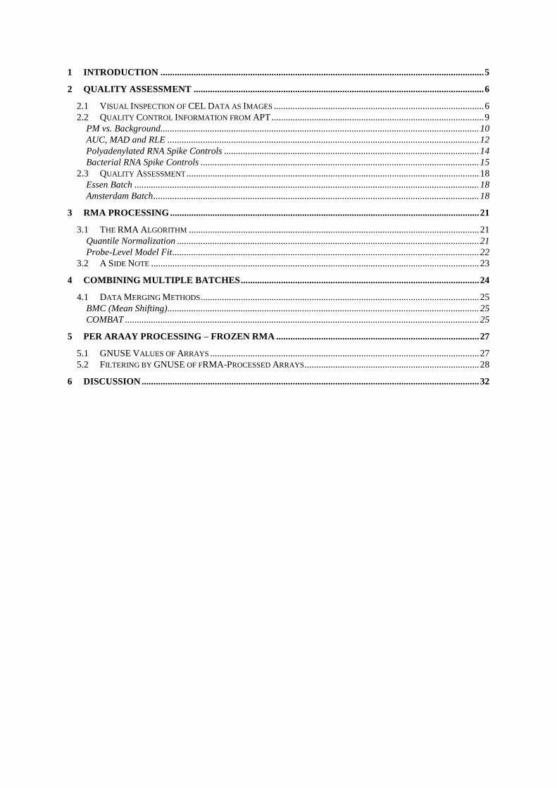
1 INTRODUCTION ......................................................................................................................................... 5

2 QUALITY ASSESSMENT ........................................................................................................................... 6

2.1 VISUAL INSPECTION OF CEL DATA AS IMAGES ......................................................................................... 6 2.2 QUALITY CONTROL INFORMATION FROM APT .......................................................................................... 9

PM vs. Background ....................................................................................................................................... 10 AUC, MAD and RLE .................................................................................................................................... 12 Polyadenylated RNA Spike Controls ............................................................................................................ 14 Bacterial RNA Spike Controls ...................................................................................................................... 15

2.3 QUALITY ASSESSMENT ............................................................................................................................ 18 Essen Batch .................................................................................................................................................. 18 Amsterdam Batch .......................................................................................................................................... 18

3 RMA PROCESSING ................................................................................................................................... 21

3.1 THE RMA ALGORITHM ........................................................................................................................... 21 Quantile Normalization ................................................................................................................................ 21 Probe-Level Model Fit .................................................................................................................................. 22

3.2 A SIDE NOTE ........................................................................................................................................... 23

4 COMBINING MULTIPLE BATCHES ..................................................................................................... 24

4.1 DATA MERGING METHODS ...................................................................................................................... 25 BMC (Mean Shifting) .................................................................................................................................... 25 COMBAT ...................................................................................................................................................... 25

5 PER ARAAY PROCESSING – FROZEN RMA ...................................................................................... 27

5.1 GNUSE VALUES OF ARRAYS .................................................................................................................. 27 5.2 FILTERING BY GNUSE OF FRMA-PROCESSED ARRAYS .......................................................................... 28

6 DISCUSSION ............................................................................................................................................... 32

5

1 INTRODUCTION

This article describes how we preprocess the expression data acquired from our Neuroblas-

toma cancer cohort with the Affymetrix Human Exon ST 1.0 arrays1. The purpose is to deliv-

er the details of our procedures, so that follow-up studies can prepare their data in a compara-

ble manner. This will allow us integrating multiple data sets together, possibly leading to new

discoveries for fighting with cancers.

Our preprocessing is composed of three main steps:

1. Quality assessment

2. RMA processing of each batch

3. Combining batches

In quality assessment, we examine the quality of individual arrays (i) via the visual inspection

of arrays as images, and (ii) using the quality information provided by the Affymetrix Power

Tools (APT). We will discuss each step in detail afterwards.

After filtering out low-quality arrays, we apply the robust multi-array algorithm (RMA) for

the arrays in each batch. Here “batch” means a collection of arrays prepared in the same con-

dition. We consider the arrays collected and processed in two different cities (Essen in Ger-

many, Amsterdam in the Netherlands) as two batches, since this level of batches has shown

significant differences.

The final step is making the RMA-processed data per batch comparable, so that we can com-

bine batches for further analyses. We choose a very simple method, which can be applied in-

dependently to each batch.

In this article we use the terms “arrays” and “chips” interchangeably. Before preprocessing,

the raw expression data of each chip is stored in a single file, with the extension “.CEL”. So a

CEL file amounts to an array or a chip.

We begin with the following chips in two batches:

Batch No. of Chips CEL Filename Prefix

Essen 113 GSM

Amsterdam 182 ITCC and NRC

Total 295 -

The Essen and Amsterdam batches contain all stages according to the International Neuro-

blastoma Staging System (INSS), and we process all stages together.

1 For details, see http://www.affymetrix.com/support/technical/byproduct.affx?product=huexon-st

6

2 QUALITY ASSESSMENT

2.1 Visual Inspection of CEL Data as Images

The first step is to literally “see” the raw data in CEL files as images. For this we can conven-

iently use the “oligo” package2 for R provided by the Bioconductor. Using this software, we

draw each CEL file as a grayscale image, and look for any spurious artifact with our eyes.

Here is an R code snippet, to plot the image corresponds to the 3rd

CEL file in /DATA:

library(oligo)

files <- list.celfiles("/DATA", full.names=TRUE)

celdata <- read.celfiles(files, pkgname="pd.huex.1.0.st.v2")

image(celdata, 3, col=gray((64:0)/64))

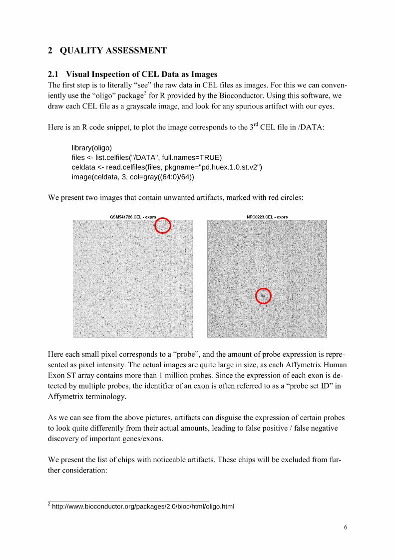
We present two images that contain unwanted artifacts, marked with red circles:

Here each small pixel corresponds to a “probe”, and the amount of probe expression is repre-

sented as pixel intensity. The actual images are quite large in size, as each Affymetrix Human

Exon ST array contains more than 1 million probes. Since the expression of each exon is de-

tected by multiple probes, the identifier of an exon is often referred to as a “probe set ID” in

Affymetrix terminology.

As we can see from the above pictures, artifacts can disguise the expression of certain probes

to look quite differently from their actual amounts, leading to false positive / false negative

discovery of important genes/exons.

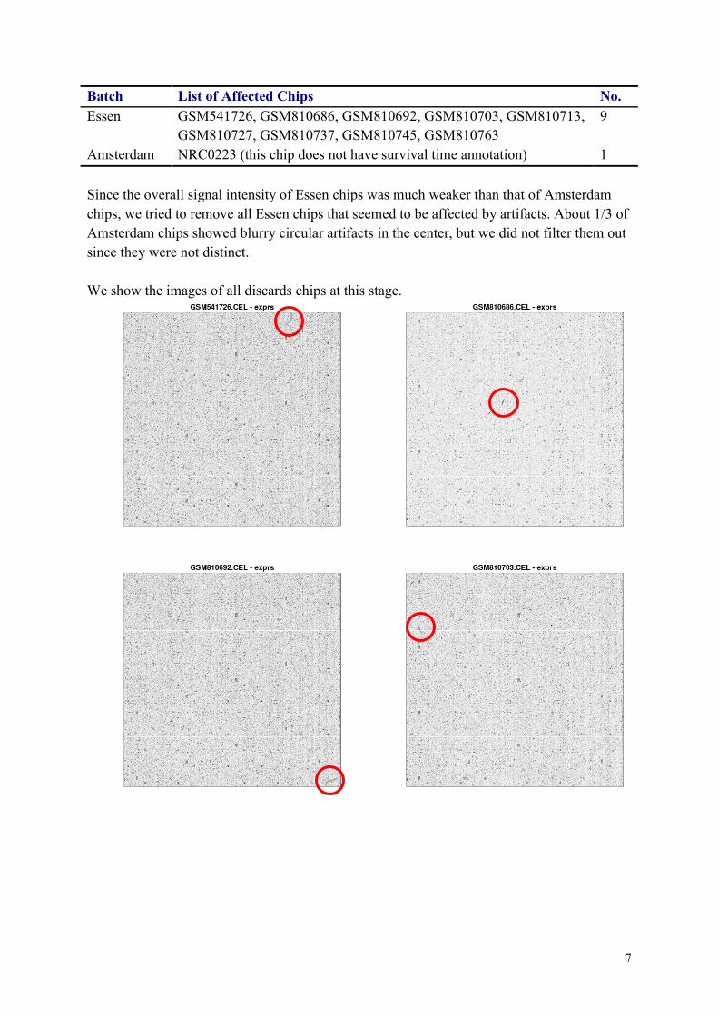
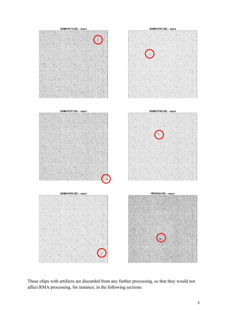
We present the list of chips with noticeable artifacts. These chips will be excluded from fur-

ther consideration:

2 http://www.bioconductor.org/packages/2.0/bioc/html/oligo.html

7

Batch List of Affected Chips No.

Essen GSM541726, GSM810686, GSM810692, GSM810703, GSM810713,

GSM810727, GSM810737, GSM810745, GSM810763

9

Amsterdam NRC0223 (this chip does not have survival time annotation) 1

Since the overall signal intensity of Essen chips was much weaker than that of Amsterdam

chips, we tried to remove all Essen chips that seemed to be affected by artifacts. About 1/3 of

Amsterdam chips showed blurry circular artifacts in the center, but we did not filter them out

since they were not distinct.

We show the images of all discards chips at this stage.

8

These chips with artifacts are discarded from any further processing, so that they would not

affect RMA processing, for instance, in the following sections.

9

2.2 Quality Control Information from APT

Given a collection of CEL files, we can use the Affymetrix Power Tools3 (APT) to create a

summary of probes in the CEL files, as well as to obtain useful quality control information

about the probes. Here a “summary” can be made either in exon-level or in transcript-level

(interchangeably, gene-level), as each exon is detected by a collection of probes, and a tran-

script (or a gene) is again a collection of exons.

We begin with the following arrays, applying APT for each batch.

Batch No. of Chips

Essen 113 – 9 (artifacts) = 104

Amsterdam 182 – 1 (artifacts) = 181

Total 285

For instance, we run APT as follows to obtain the exon-level summary of probes and the

quality control information of Essen chips:

apt-probeset-summarize \

-p HuEx-1_0-st-v2.r2.pgf \

-c HuEx-1_0-st-v2.r2.clf \

-b HuEx-1_0-st-v2.r2.antigenomic.bgp \

--qc-probesets HuEx-1_0-st-v2.r2.qcc \

-s HuEx-1_0-st-v2.r2.dt1.hg18.core.ps \

-a rma \

-o output_dir \

./ESSEN/*.CEL

Here the “-s” option specifies the category of exon-level summary we make about probes.

The exons are categorized into “core”, “extended”, “full”, “free”, and “ambiguous”, by the

decreasing order of evidence we have about them. In this article we focus on the core exons.

For gene-level summaries, the “-s” option is replaced by “-m”. For example, to create core

gene-level summary, we use

-m HuEx-1_0-st-v2.r2.dt1.hg18.core.mps

We refer to an introductory article (Lockstone 2011) for details about the options and the

Affymetrix library and meta probe set information files.

The above command generates two tab-separated text files in the output_dir:

rma.summary.txt : the summary of probes in a specified category.

3 APT version 1.15.0, the latest release at the time of writing, is available at

http://www.affymetrix.com/partners_programs/programs/developer/tools/powertools.affx

10

rma.report.txt : the quality control information of arrays

The quality control information is generated only if we specify the “--qc-probesets” option.

In usual cases, the options above are all we need. More details about the options can be found

on the APT online manual (Affymetrix 2007a).

In this section we describe how we use the quality control information. The output from APT

provides many characteristics about the input arrays, and we focus a few of them that we

consider significant. Note that after finding out low-quality arrays, we will run APT again to

make summaries, excluding these low-quality arrays. We believe such exclusion is important

since low-quality arrays are likely to have adverse effect on summary outcomes, especially

for the popular robust multi-array analysis (RMA) algorithm (Irizarry 2003).

We follow a white paper from Affymetrix (Affymetrix 2007b) for quality assessment of ar-

rays based upon the information from APT.

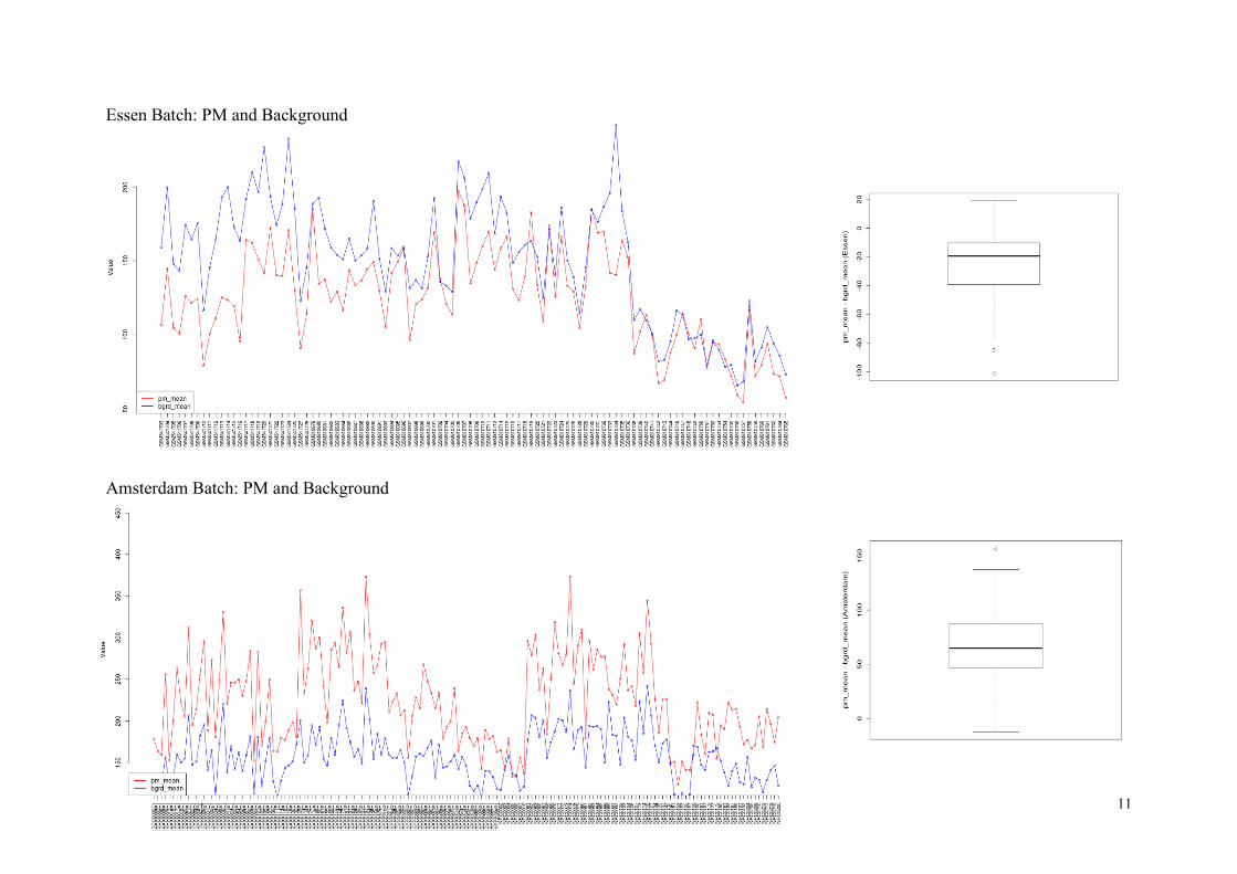
PM vs. Background

First of all, we examine the signal strength of probes. For this we use two sets of values from

the quality information:

pm_mean: the averaged raw intensity values of PM (perfect match) probes.

bgrd_mean: the averaged raw intensity values of background probes.

The “pm_mean” and “bgrd_mean” are also the corresponding column names of the quality

information table in the rma.report.txt file. These values are about the raw intensity values,

prior to any transformation.

The pm_mean values can be used to find chips that are too bright: being too bright is not a

problem by itself because algorithms such as RMA can handle it to a certain degree, but it

tells us that a closer look would be necessary. Also, in usual cases, the pm_mean and

bgrd_mean values are positively correlated. So low pm_mean with high bgrd_mean values

may indicate low quality. But as these are only indicative measures, we only use them to find

arrays with possible issues.

The next plots show pm_mean and bgrd_mean values for two batches, Essen and Amterdam.

The pm_mean values range over 50~200 in the Essen batch, and over 100~400 in the Am-

sterdam batch. We mark the Essen chips with pm_mean < 100, as well as the two Essen chips

with seemingly anti-correlated pm/bg values (outliers in the boxplots), for further inspection.

All Amsterdam chips were fine with these criteria.

11

Essen Batch: PM and Background

Amsterdam Batch: PM and Background

12

The arrays marked for closer look is listed here:

Criteria List of Arrays No

pm_mean < 100

GSM541710, GSM541716, GSM541727, GSM810697, GSM810738,




GSM810761, GSM810762, GSM810764, GSM810765

24

anti-correlation GSM541720, GSM810734 2

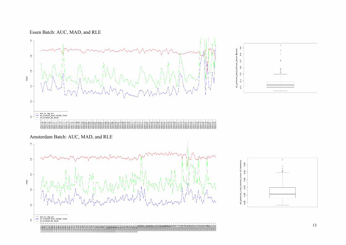
AUC, MAD and RLE

Here we use three quality measures, pos_vs_neg_auc, all_probeset_mad_residual_mean, and

all_probeset_rle_mean (we also call them as “auc”, “mad”, and “rle”, respectively).

The pos_vs_neg_auc (auc) is the area under the ROC curve, comparing signal values for pos-

itive control to the negative control probe sets. The AUC value of 1.0 reflects perfect separa-

tion of two probe sets, whereas the value of 0.5 indicates no separation. Typical auc values in

Affymetrix arrays are between 0.8 and 0.9.

The all_probeset_mad_residual_mean (mad) is the mean value of the absolute deviation of

probes from the median. Here “all_probeset” stands for the probes in a specific category,

which are “core exons” in our case. The mad values tell us the difference between the actual

and the predicted values by a model used in the processing algorithm (e.g. RMA). So excep-

tionally high mad values would indicate problems in the corresponding chips.

The all_probeset_rle_mean (rle) is the mean value of the absolute relative log expression

(RLE) for all core exon probe sets, which is defined by

( ) ( | ( ) ( )| )

The RLE values are averaged over probes in each array to produce the all_probeset_rle_mean

value. This shows the variability in expression of each array, which could come from meas-

urement error but also from sheer biological variation.

In the next page, we show the plots of the three quality measures.

13

Essen Batch: AUC, MAD, and RLE

Amsterdam Batch: AUC, MAD, and RLE

14

Overall, the auc values (red curves) are higher in Essen chips (mean 0.86) than in Amsterdam

chips (mean 0.83), although Essen chips look much brighter than Amsterdam chips. Consid-

ering the typical auc values in 0.8~0.9, we choose the threshold rule (auc < 0.8) to detect low-

quality arrays. Here are the lists:

Batch

(criterion)

List of Arrays No.

Essen

(auc < 0.8)

GSM810759, GSM810765

(both are in our bad-chip candidate due to pm_mean < 100)

2

Amsterdam

(auc < 0.8)

ITCC0008E1, ITCC0036E1, ITCC0063E1, ITCC0109E1, ITCC0111E1,

ITCC0151E1, ITCC0546E1, ITCC0549E1, ITCC0552E1,

ITCC0558E1, NRC0152, NRC0172, NRC0173, NRC0204

14

Next, we investigate the mad values (blue curves). Seeing the outliers in the two boxplots of

mad values above, we choose a reasonable threshold (mad > 0.5) for detection.

Batch

(criterion)

List of Arrays No.

Essen

(mad > 0.5)



GSM810765

11

Amsterdam

(mad > 0.5)

None 0

Finally, for the rle values, it is not as straightforward as the two previous quality measures to

define a good threshold, since high rle values could be from meaningful biological differ-

ences. Therefore we do not use the rle values for filtering, but as we can see in the plots

above, almost all chips with unusually high rle values are already removed by the mad > 0.5

criterion in the Essen batch, and by auc < 0.8 criterion in the Amsterdam batch.

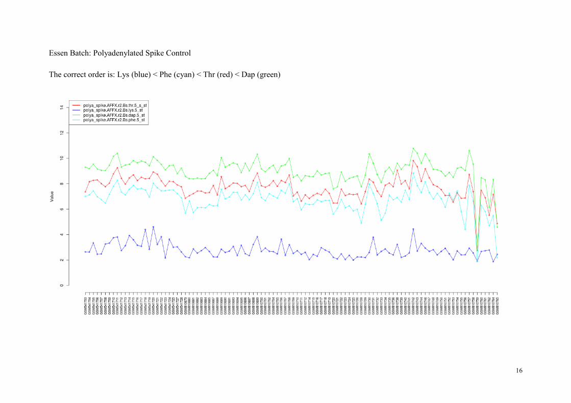
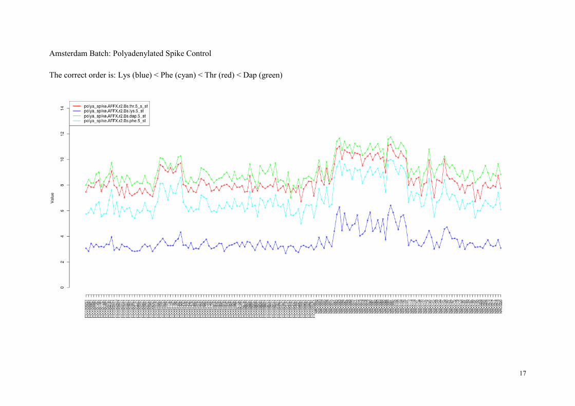
Polyadenylated RNA Spike Controls

The polya_spike probes consist of four sets of polyadenylated RNA spike probes (Lys, Phe,

Thr, and Dap). The RNA sequences of these probes do not appear in humans, and therefore

we can use them for quality control. The polya_spike probes are designed to detect errors in

the target preparation stage of microarray experiments.

15

In normal situation, the expression of polya_spike control probes should follow the following

order:

● polya_spike : Lys < Phe < Thr < Dap.

The spike control probes typically show higher variability across arrays than other quality

measures as they are shorter in length, but it is unimportant since we only examine the rank

order of four probe sets in individual arrays.

We have found few arrays that do not preserve the correct order:

Batch (criterion) List of Arrays No.

Essen

(polya_spike)

GSM810752, GSM810753, GSM810754, GSM810759,

GSM810765

5

Amsterdam

(polya_spike)

ITCC0544E1

1

In the next page we show the plots of polya_spike control probes for two batches.

Bacterial RNA Spike Controls

The bac_spike is another set of spike control probes, comprising of four subsets that hybrid-

ize to the pre-labeled bacterial RNA spike control probes (BioB, BioC, BioD, and Cre). This

category is useful for detecting problems in the hybridization phase or in the arrays them-

selves.

The usage of bac_spike control is similar to polya_spike. In normal situations, the expression

of bac_spike probes should follow the predetermined order:

● bac_spike : BioB < BioC < BioD < Cre

There was no array in our data which showed incorrect bac_spike rank order.

16

Essen Batch: Polyadenylated Spike Control

The correct order is: Lys (blue) < Phe (cyan) < Thr (red) < Dap (green)

17

Amsterdam Batch: Polyadenylated Spike Control

The correct order is: Lys (blue) < Phe (cyan) < Thr (red) < Dap (green)

18

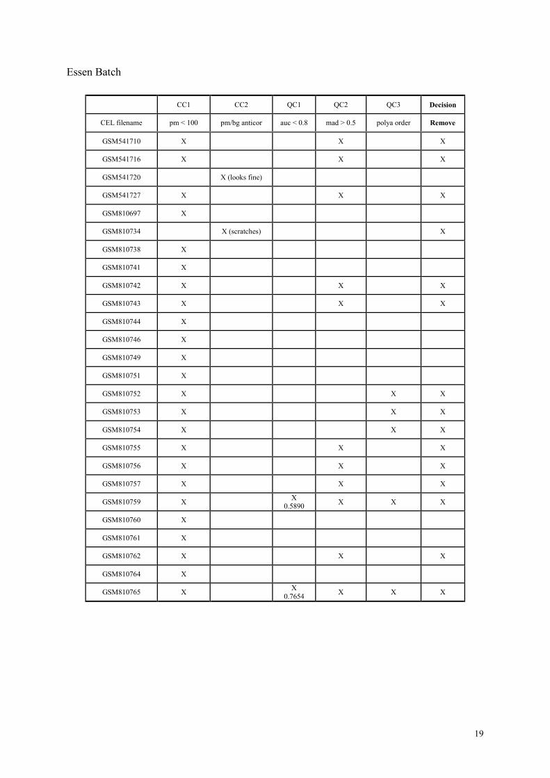
2.3 Quality Assessment

Now we combine the information we have gathered in Section 2.2, and determine the arrays

to exclude because of their inferior measurement quality.

For concise description, we name the two criteria for detecting possibly low-quality chips:

CC1 (candidate criterion 1): pm_mean < 100, and

CC2 (candidate criterion 2): pm/bgrd anti-correlation.

Similarly, the three more definitive quality criteria are called as follows:

QC1 : auc < 0.8,

QC2: mad > 0.5, and

QC3: polya_spike has incorrect rank ordering.

Essen Batch

First, for the candidates due to CC1, we exclude the chips that are also detected by any one of

the three quality criteria, Q1, Q2, and Q3.

Next, for the candidates due to CC2, we there was no outstanding problem in terms of QC1,

QC2, or QC3. Then we investigated the CEL file images again, and found one of the two

candidates had visible scratches. We thus excluded this chip, but did not exclude the other

that showed no visible artifacts.

To conclude, we removed 15 chips from the Essen batch, in addition to the ones that have

already removed by visual inspection.

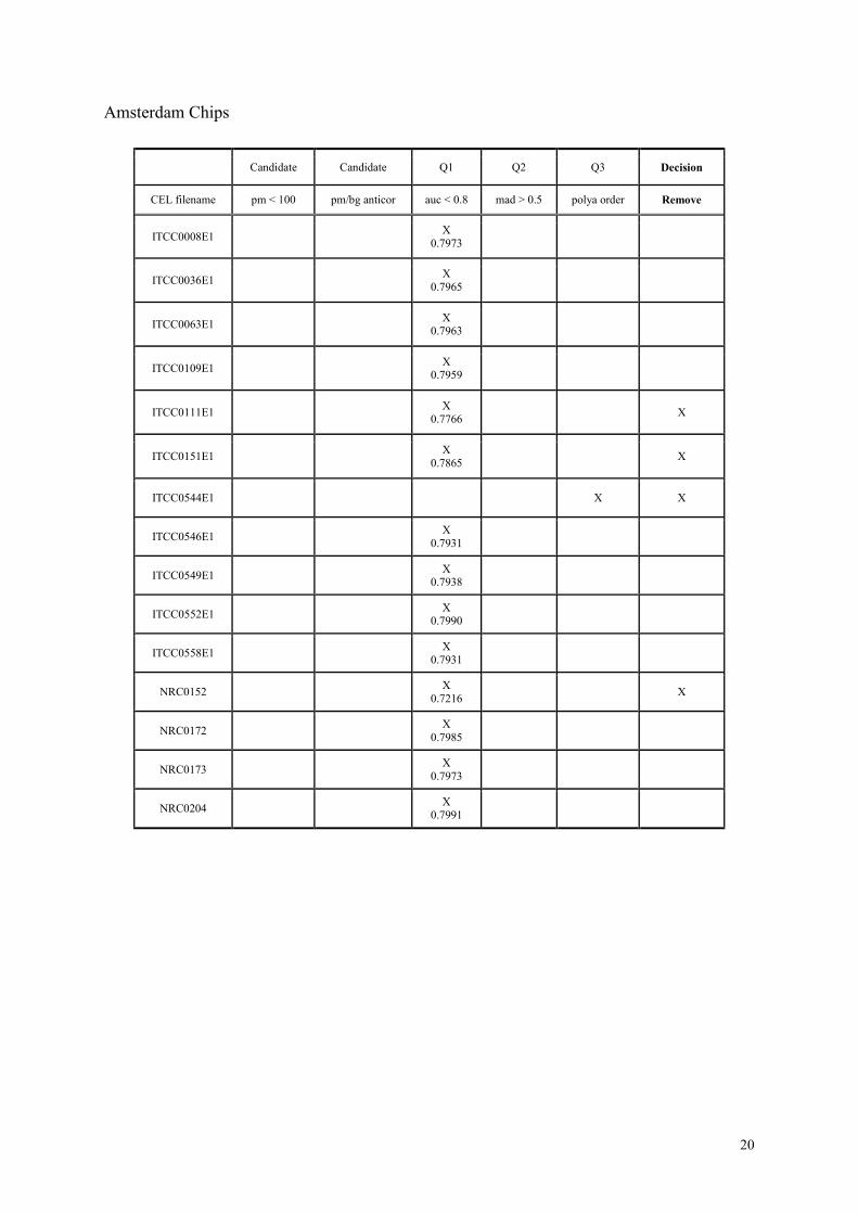
Amsterdam Batch

Among the Amsterdam arrays, we only had the ones detected by QC1 and QC3. In fact, for

QC1, the auc values were very close (about 0.79) to the threshold value of 0.80. Therefore we

have removed only the chips that had auc values strictly less than 0.79. We had a single chip

detected by QC3, having incorrect order in the polya_spike category. We removed this chip

as well.

To conclude, we removed 4 chips from the Amsterdam batch, in addition to the ones that

have removed by visual inspection.

The tables in the following pages summarize the situation.

19

Essen Batch

CC1 CC2 QC1 QC2 QC3 Decision

CEL filename pm < 100 pm/bg anticor auc < 0.8 mad > 0.5 polya order Remove

GSM541710 X X X

GSM541716 X X X

GSM541720 X (looks fine)

GSM541727 X X X

GSM810697 X

GSM810734 X (scratches) X

GSM810738 X

GSM810741 X

GSM810742 X X X

GSM810743 X X X

GSM810744 X

GSM810746 X

GSM810749 X

GSM810751 X

GSM810752 X X X

GSM810753 X X X

GSM810754 X X X

GSM810755 X X X

GSM810756 X X X

GSM810757 X X X

GSM810759 X X

0.5890 X X X

GSM810760 X

GSM810761 X

GSM810762 X X X

GSM810764 X

GSM810765 X X

0.7654 X X X

20

Amsterdam Chips

Candidate Candidate Q1 Q2 Q3 Decision

CEL filename pm < 100 pm/bg anticor auc < 0.8 mad > 0.5 polya order Remove

ITCC0008E1 X

0.7973

ITCC0036E1 X

0.7965

ITCC0063E1 X

0.7963

ITCC0109E1 X

0.7959

ITCC0111E1 X

0.7766 X

ITCC0151E1 X

0.7865 X

ITCC0544E1 X X

ITCC0546E1 X

0.7931

ITCC0549E1 X

0.7938

ITCC0552E1 X

0.7990

ITCC0558E1 X

0.7931

NRC0152 X

0.7216 X

NRC0172 X

0.7985

NRC0173 X

0.7973

NRC0204 X

0.7991

21

3 RMA PROCESSING

At this point we have discarded all arrays that have been classified as of low quality. We ap-

ply the RMA algorithm again for the remaining arrays, to make gene or exon level summar-

ies for further analysis. The numbers of arrays look as follows:

Batch No. of Chips

Essen 113 – 9 (artifacts) – 15 (quality) = 89

Amsterdam 182 – 1 (artifacts) – 4 (quality) = 177

Total 266

We run the robust multi-array analysis (RMA) algorithm (Irizarry 2003) for each batch sepa-

rately, using the Affymetrix Power Tools (APT). Since the model used in the RMA algorithm

assumes that the distribution of each probe is similar across all input arrays, which is often

not true for arrays in different batches, it is desirable to apply RMA on each batch separately.

In our case, the overall signal intensity of the Essen batch was much lower (dimmer images)

than that of the Amsterdam batch, so we applied RMA separately for each batch.

3.1 The RMA Algorithm

For better understanding, we briefly introduce the RMA algorithm. RMA consists of (1)

background correction, (2) quantile normalization, (3) transformation, and (4) fitting a

linear model to take advantage of “probe effect”, that the variability between probes of a

probe set in an array is typically larger than the variability of an individual probe across ar-

rays. We focus on the steps (2) and (4) since others are straightforward.

Quantile Normalization

The goal of the step (2) is to make the distribution of probe intensities the same across, say, n

arrays. This can be done by quantile normalization (Bolstad 2003). Let

( ) be the vector of the kth quantiles for n arrays. To make the kth quan-

tiles the same for all arrays, we project on the n-dimensional diagonal vector

(

√

√ ), to obtain

(

∑

∑

)

That is, we can substitute the original values by their corresponding mean quantiles. We can

write a simple algorithm for doing this:

22

1. Given n arrays with p features, construct a matrix X by putting arrays as columns.

2. Sort each column of X, producing Xsort.

3. For each row of Xsort, take the mean, and replace the row elements with the mean.

4. Rearrange Xsort so to have the same ordering as the X.

Since the original probe intensity values are replaced by mean values at each quantile, it

would be undesirable to process arrays with genomic difference at the same time. For in-

stance, if we have arrays for which the probes corresponding to gene A and B have their

quantile orders exchanged, then the means can be taken mixing the expression of A and B.

Probe-Level Model Fit

After background correction, quantile normalization, and log2 transformation, the probe-level

intensity values are used to find linear model fits (McCall 2010),

for probes in probe sets on arrays . Here represents the

expression of a probe set s on an array i, is the probe effect for the jth probe of the probe

set s. The last term represents measurement error. The purpose of this model is to capture the

variability of probes in each probe set. After fitting the model, RMA reports the estimate ̂

as the final outcome.

To make the parameters identifiable, we assume that ∑ for each probe set s. This

can be seen as assuming that on average, the probes measure the true expression. A popular

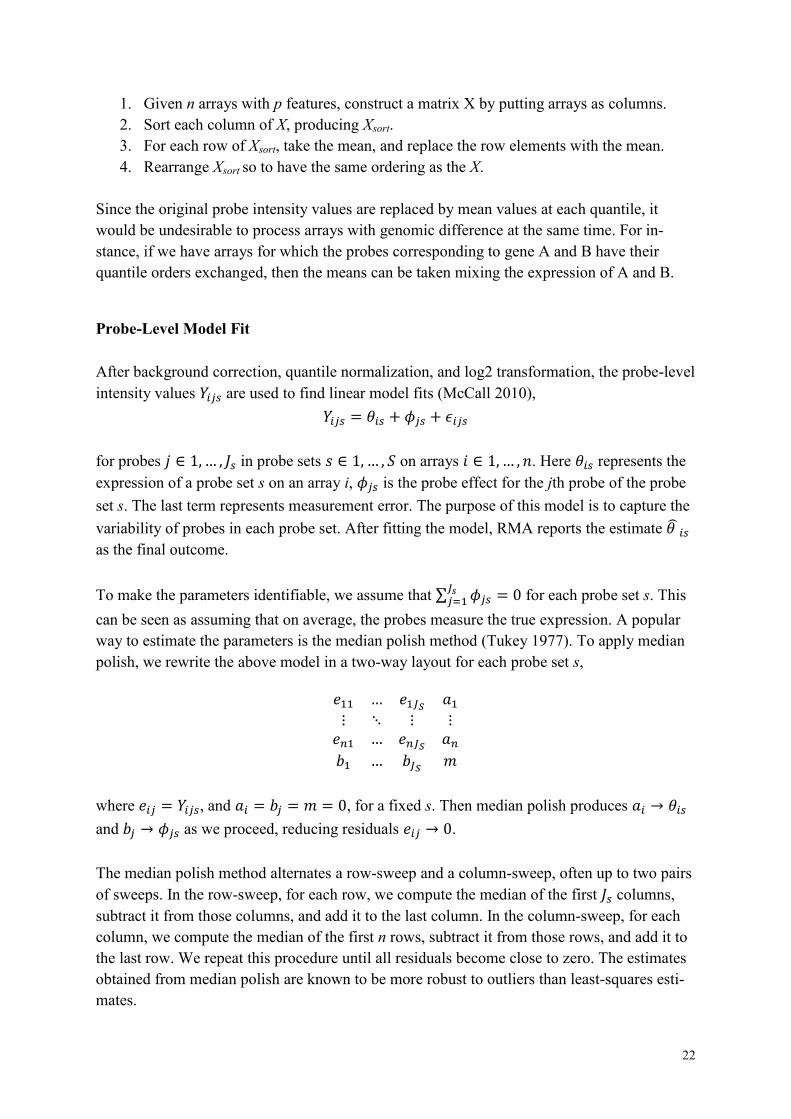
way to estimate the parameters is the median polish method (Tukey 1977). To apply median

polish, we rewrite the above model in a two-way layout for each probe set s,

where , and , for a fixed s. Then median polish produces

and as we proceed, reducing residuals .

The median polish method alternates a row-sweep and a column-sweep, often up to two pairs

of sweeps. In the row-sweep, for each row, we compute the median of the first columns,

subtract it from those columns, and add it to the last column. In the column-sweep, for each

column, we compute the median of the first n rows, subtract it from those rows, and add it to

the last row. We repeat this procedure until all residuals become close to zero. The estimates

obtained from median polish are known to be more robust to outliers than least-squares esti-

mates.

23

3.2 A Side Note

There are several arrays for which we do not have valid survival time annotation:

Chips without survival time annotation (7 chips): ITCC0533E1, ITCC0551E1,

NRC0009, NRC0099, NRC0100, NRC0109, NRC0110.

Chips with too short (< 5 days) survival time without an event (11 chips): NRC0064,

NRC0075, NRC0077, NRC0087, NRC0088, NRC0090, NRC0098, NRC0203,

NRC0208, NRC0209, NRC0225.

Also, there are four arrays that pass all quality tests, but show unusually high

all_probeset_rle_mean values: NRC0005, NRC0135, NRC0175, NRC0204.

We do not exclude these chips in the RMA processing.

24

4 COMBINING MULTIPLE BATCHES

Our final step of microarray preprocessing is to make multiple batches comparable to each

other. This step is necessary because (i) we prefer to have large number of arrays in down-

stream analyses whenever possible, but creating a single large batch is impractical, and (ii) if

we apply RMA separately on multiple input array sets, then the resulting sets are not likely to

be comparable since a local reference distribution is made from given data in each quantile

normalization step of RMA. In addition, (iii) in order to classify new patients using a predic-

tor learned from training data, we have to make the data from new patients comparable to the

training data. Otherwise, the predictor would not work.

For convenience, we call the method that makes multiple (RMA-processed) batches compa-

rable as a data combining (or a data merging) method. We prefer to choose a data merging

method that is applicable for each batch independently, especially for the batches from new

patients.

We should mention that there is a possible alternative for multi-array summarizing, called the

frozen RMA (McCall 2010), which produces comparable outcomes even if we apply it per

batch or per array. The difference of fRMA to RMA is that fRMA makes use of a global ref-

erence created from publicly available expression arrays, instead of a local reference from

input arrays. Therefore no data merging is required after applying fRMA. We found that

fRMA worked fine for gene chips, but unfortunately not for exon arrays. We expect that the

performance of fRMA will improve with more exon arrays available in public.

It is a common practice is to apply RMA for all arrays in a study. However, this may not be

preferable in several aspects: (i) if there are arrays with permuted probe distributions, then

quantile normalization in RMA could make averages over probes corresponding to different

genes/exons, (ii) lumping arrays together in order to cancel out batch effects is not a good

idea, since RMA does not explicitly deal with any batch effect4, and (iii) in principle, test da-

ta should be prepared separately.

In a strict sense, the arrays that are processed at the exactly same condition should define a

batch. However, the size of such batches is quite small (24~96) due to technical limitations,

and we often do not keep the corresponding batch information. In this article, we consider

batches in terms of two processing locations, Essen and Amsterdam, since our arrays look

most significantly different at this level of separation. So, strictly speaking, our batch stands

for an experiment, a collection of batches.

In the following we make a short survey of the data merging methods that look the most

plausible for our purpose

4 A simple 3-D projection of data using PCA often reveals this fact.

25

4.1 Data Merging Methods

There are only handful approaches for making data from multiple batches comparable. A col-

lection of them can be found, for example, in an R package called “inSilicoMerging”5.

We introduce three methods, SIMPLE, BMC and COMBAT, using their names in the inSili-

coMerging package. The SIMPLE method just combines batches together without any trans-

formation.

BMC (Mean Shifting)

This method makes each exon expression centered at the zero value, by subtracting the mean

expression of each exon over arrays from the expression value of the exon, per batch. This

method does not perform any scaling (by standard deviation, for example). No scaling might

be preferable in our case, since (i) RMA-processed data usually have similar scale, and (ii)

scaling may conceal biological variability. It is reported that this method can cancel multipli-

cative systematic bias (Sims 2008).

The merit of this method is that we can apply it completely independently on each batch.

COMBAT

COMBAT is an empirical Bayesian approach that tries to estimate and cancel batch effects

(Johnson 2007). This method is known to work better than other merging methods when the

sizes of batches are small (< 25). In our case, we cannot find any significant difference to the

simpler alternative, BMC. Also, COMBAT requires to “see” all batches at once, and thus it

cannot be applied separately for each batch.

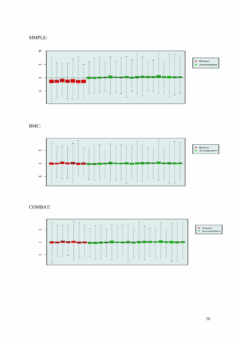
In the next page we show the mean RLE (relative log expression) values of 25 arrays ran-

domly selection from the Essen and Amsterdam batches, after merging the data by SIMPLE,

BMC, and COMBAT, respectively. Clearly, BMC and COMBAT make the intensity values

more similar across batches, compared to SIMPLE. Comparison between BMC and

COMBAT is less obvious.

In conclusion, we choose the BMC (mean shifting) method for combining our batches.

5 http://www.bioconductor.org/packages/2.11/bioc/html/inSilicoMerging.html

26

SIMPLE:

BMC:

COMBAT:

27

5 PER ARRAY PROCESSING – FROZEN RMA

The preprocessing approach we have discussed so far has several caveats: (1) it requires to

apply the algorithm again for the entire arrays whenever new arrays arrive, and (2) it is not

straightforward which algorithm to choose for merging RMA-processed batches of data.

An alternative of RMA is the frozen RMA (McCall 2010). In addition to the probe effects,

fRMA is designed to handle probe-specific random effects. Comparing to RMA, fRMA

makes use of a global reference, instead of a reference distribution estimated from input ar-

rays. The global reference is platform specific, and obtained from a large number of arrays

available in public (GEO, for example).

In this report, we use the fRMA package in Bioconductor (version 1.11.0) with the global

reference package for human exon arrays, huex.1.0.st.v2frmavecs (version 0.0.4).

There is a useful addendum to fRMA, called GNUSE (global normalized unscaled standard

error), which allows us to assess the quality of individual arrays (M. McCall 2011). Here we

use only GNUSE scores to access array quality, without performing visual inspection and

filtering by quality measures provided by the APT (Affymetrix Power Tools).

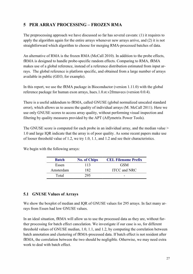
The GNUSE score is computed for each probe in an individual array, and the median value >

1.0 and large IQR indicate that the array is of poor quality. As some recent papers make use

of looser threshold value of 1.2, we try 1.0, 1.1, and 1.2 and see their characteristics.

We begin with the following arrays:

Batch No. of Chips CEL Filename Prefix

Essen 113 GSM

Amsterdam 182 ITCC and NRC

Total 295 -

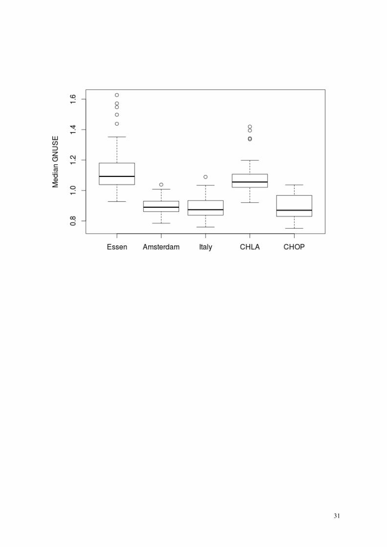
5.1 GNUSE Values of Arrays

We show the boxplot of median and IQR of GNUSE values for 295 arrays. In fact many ar-

rays from Essen had low GNUSE values.

In an ideal situation, fRMA will allow us to use the processed data as they are, without fur-

ther processing for batch effect cancelation. We investigate if our case is so, for different

threshold values of GNUSE median, 1.0, 1.1, and 1.2, by computing the correlation between

batch annotation and clustering of fRMA-processed data. If batch effect is not resident after

fRMA, the correlation between the two should be negligible. Otherwise, we may need extra

work to deal with batch effect.

28

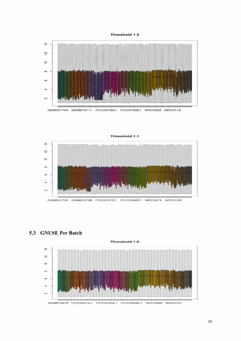
5.2 Filtering by GNUSE of fRMA-Processed Arrays

Here we summarize the arrays to be filtered for three threshold values.

Threshold for

median

GNUSE val-

ues

No. of ar-

rays to be

removed

Arrays

1.2 21 GSM541703, GSM541705, GSM541706, GSM541710, GSM541711, GSM541712,

GSM541716, GSM541727, GSM810686, GSM810727, GSM810742, GSM810743,


GSM810762, GSM810764, GSM810765









GSM810761, GSM810762, GSM810763, GSM810764, GSM810765
















29


GSM810765, ITCC0003E1, ITCC0111E1, ITCC0114E1, NRC0145, NRC0151, NRC0152,

NRC0155, NRC0157

We show the plots of exon expression after fRMA processing, for the three threshold values

of median GNUSE in the next page. As we can see, there are few arrays still remaining after

filtering with the threshold values 1.2 and 1.1, that have quite different median expression

compared to the others. For the threshold value 1.0 however, median expression values seem

alike.

We compute the correlation between the batch annotation (a vector of 1, 2, and 3 correspond-

ing to “GSM”, “ITC” and “NRC” arrays) and the kmeans clustering result (a vector of cluster

assignment, in our case mostly 1 to “GSM”, 2 to “ITC” and 3 to “NRC”). High correlation

between the two vectors suggests that the fRMA-processed data still has high correlation to

the batches.

Threshold 1.2 1.1 1.0

Correlation 0.81 0.58 0.23

In this respect, the threshold value of 1.0 appears to be the best choice, except for the fact that

it removes almost all arrays from the Essen batch.

No. of Arrays with

Prefixes

GSM ITCC NRC

Before Filtering 113 92 90

After Filtering

(threshold = 1.0)

16 89 85

30

5.3 GNUSE Per Batch

31

32

6 DISCUSSION

We present our data preprocessing steps for microarrays experiments. Our goal is to obtain as

clean as possible data for further analyses, since the number of arrays is often not large

enough to make atypical cases negligible. The importance of careful preprocessing is empha-

sized in lectures and textbooks, but it appears to be ignored in practice surprisingly often.

Many steps in preprocessing require human intervention and experience, which might have

contributed to insufficient attention to preprocessing. Developing computer software for

some of the tasks would help the community therefore, for instance, to automatize visual in-

spection of arrays based on computer vision or machine learning technology.

There is also room for improvement in the algorithms creating probe summaries, such as

RMA or fRMA. For example, the quantile normalization step in RMA has an underlying as-

sumption that the rank order of probe intensity values would not change across input arrays.

However, it is often the case we have a collection of arrays consists of unknown genotype

subgroups, where different subgroups are expected to have different rank orders of probe ex-

pression.

We hope that researchers and students may find this article helpful for preparing their micro-

array data.

33

BIBLIOGRAPHY

Affymetrix. Affymetrix Power Tools: VIGNETTES: Use of APT to Analyze WT Based Exon and Gene Expression Arrays. May 31, 2007a. http://media.affymetrix.com/support/developer/powertools/changelog/VIGNETTE-wt-analysis.html (accessed November 27, 2012).

—. "Quality Assessment of Exon and Gene Arrays." Quality Assessment of Exon and Gene Arrays. April 6, 2007b. http://media.affymetrix.com/support/technical/whitepapers/exon_gene_arrays_qa_whitepaper.pdf (accessed November 27, 2012).

Bolstad, B.M. and Irizarry, R.A and Astrand, M. and Speed, T.P. "A comparison of normalization methods for high density oligonucleotide array data based on variance and bias." Bioinformatics 19, no. 2 (2003): 185-193.

Irizarry, Rafael A. and Bolstad, Benjamin M. and Collin, Francois and Cope, Leslie M. and Hobbs, Bridget and Speed, Terence P. "Summaries of Affymetrix GeneChip probe level data." Nucleic acids research 31, no. 4 (2003): e15.

Johnson, W. Evan and Li, Cheng and Rabinovic, Ariel. "Adjusting batch effects in microarray expression data using empirical Bayes methods." Biostatistics 8, no. 1 (2007): 118-127.

Lockstone, Helen E. "Exon array data analysis using Affymetrix power tools and R statistical software." Briefings in Bioinformatics 12, no. 6 (2011): 634-644.

M. McCall, P. Murakami, M. Lukk, W. Huber, R. Irizarry. "Assessing affymetrix GeneChip microarray quality." BMC Bioinformatics 12, no. 1 (2011): 137.

McCall, Matthew N. and Bolstad, Benjamin M. and Irizarry, Rafael A. "Frozen robust multiarray analysis (fRMA)." Biostatistics 11, no. 2 (2010): 242-253.

Sims, Andrew and Smethurst, Graeme and Hey, Yvonne and Okoniewski, Michal and Pepper, Stuart and Howell, Anthony and Miller, Crispin and Clarke, Robert. "The removal of multiplicative, systematic bias allows integration of breast cancer gene expression datasets - improving meta-analysis and prediction of prognosis." BMC Medical Genomics 1, no. 1 (2008): 42.

Tukey, John W. Exploratory Data Analysis. : Addison-Wesley, 1977.

Documents

Sangkyun Lee Alexander Schramm Technical Report · Sangkyun Lee Alexander Schramm ... . ... The first step is to literally “see” the raw data in CEL files as images