Embed Size (px)
Citation preview
AnIntroduction to
SLE
ChristianBeneš
Part IReferences
Discrete Models
The LoewnerEquation
Part IISLE, the NaturalCandidate
Convergence ofdiscrete models toSLE
Applications
ConformalRestriction
Brownian loop area
Non-intersectionExponents
Brownian Frontier,etc.
An Introduction to the Schramm-LoewnerEvolution
Christian Beneš
Mathematics DepartmentCity University of New York, Brooklyn College
CUNY Probability SeminarNovember 22, 2011
AnIntroduction to
SLE
ChristianBeneš
Part IReferences
Discrete Models
The LoewnerEquation
Part IISLE, the NaturalCandidate
Convergence ofdiscrete models toSLE
Applications
ConformalRestriction
Brownian loop area
Non-intersectionExponents
Brownian Frontier,etc.
Outline
1 Part IReferencesDiscrete ModelsThe Loewner Equation
2 Part IISLE, the Natural CandidateConvergence of discrete models to SLEApplications
Conformal RestrictionBrownian loop areaNon-intersection ExponentsBrownian Frontier, etc.
AnIntroduction to
SLE
ChristianBeneš
Part IReferences
Discrete Models
The LoewnerEquation
Part IISLE, the NaturalCandidate
Convergence ofdiscrete models toSLE
Applications
ConformalRestriction
Brownian loop area
Non-intersectionExponents
Brownian Frontier,etc.
References
1 Conformally Invariant Processes in the Plane by GregLawler
2 Random planar curves and Schramm-Loewnerevolutions by Wendelin Werner:http://arxiv.org/abs/math/0303354
3 Scaling Limits and SLE by Greg Lawler:http://www.math.uchicago.edu/~lawler/papers.html
4 Numerous (technical) papers, by Lawler, Schramm,Werner, Smirnov, Beffara, Duminil-Copin, Dubédat,Hongler, Chelkak, Nolin, Camia, Newman, Rohde,Sheffield, Zhang, Garban, Trujillo-Ferreras, Kozdron,Alberts, Johansson-Viklund, Beneš, etc. (my apologiesto anyone whose name should be here but wasomitted!)
AnIntroduction to
SLE
ChristianBeneš
Part IReferences
Discrete Models
The LoewnerEquation
Part IISLE, the NaturalCandidate
Convergence ofdiscrete models toSLE
Applications
ConformalRestriction
Brownian loop area
Non-intersectionExponents
Brownian Frontier,etc.
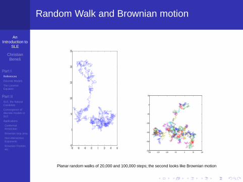
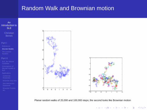
Random Walk and Brownian motion
−80 −60 −40 −20 0 20 40 60−50
0
50
100
150
200
250
−200 −150 −100 −50 0 50 100−250
−200
−150
−100
−50
0
50
Planar random walks of 20,000 and 100,000 steps; the second looks like Brownian motion
AnIntroduction to
SLE
ChristianBeneš
Part IReferences
Discrete Models
The LoewnerEquation
Part IISLE, the NaturalCandidate
Convergence ofdiscrete models toSLE
Applications
ConformalRestriction
Brownian loop area
Non-intersectionExponents
Brownian Frontier,etc.
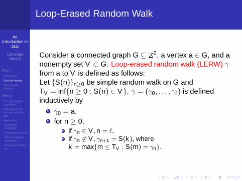
Statistical Mechanics and Conformal Invariance
Brownian motion is the scaling limit of a large class ofrandom walks on various lattices. This is an example ofuniversality.One of the key features of planar Brownian motion isconformal invariance:Consider a domain 0 ∈ D ( C and Brownian motion runfrom the origin until it hits the boundary B[0, τ ]. Then ifφ : D → D′ is a conformal map with φ(0), there is a timechange T : [0, σ] → [0, τ ] such that φ(B[T (s),0 ≤ s ≤ σ])has the same distribution as Brownian motion in D′ from theorigin to ∂D′.Physicists have long predicted that many other discretemodels should satisfy properties of universality and (in theirscaling limits) conformal invariance. They include the Isingmodel, percolation, self-avoiding walk, loop-erased randomwalk, etc.
AnIntroduction to
SLE
ChristianBeneš
Part IReferences
Discrete Models
The LoewnerEquation
Part IISLE, the NaturalCandidate
Convergence ofdiscrete models toSLE
Applications
ConformalRestriction
Brownian loop area
Non-intersectionExponents
Brownian Frontier,etc.
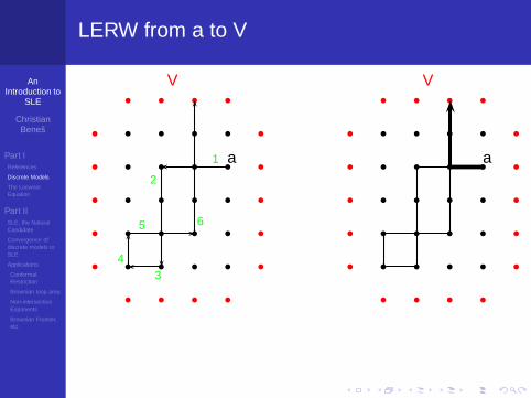
Loop-Erased Random Walk
Consider a connected graph G ⊆ Z2, a vertex a ∈ G, and anonempty set V ⊂ G. Loop-erased random walk (LERW) γfrom a to V is defined as follows:Let S(n)n≥0 be simple random walk on G andTV = infn ≥ 0 : S(n) ∈ V. γ = (γ0, . . . , γℓ) is definedinductively by
γ0 = a,for n ≥ 0,
if γn ∈ V , n = ℓ,if γn 6∈ V , γn+1 = S(k), wherek = maxm ≤ TV : S(m) = γn.
AnIntroduction to
SLE
ChristianBeneš
Part IReferences
Discrete Models
The LoewnerEquation
Part IISLE, the NaturalCandidate
Convergence ofdiscrete models toSLE
Applications
ConformalRestriction
Brownian loop area
Non-intersectionExponents
Brownian Frontier,etc.
LERW from a to V
b b b b
b b b b
b b b b
b b b b
b b b b
b b b b
b b b b
b
b
b
b
b
b
b
b
b
b
a
V
1
2
34
5 6
b b b b
b b b b
b b b b
b b b b
b b b b
b b b b
b b b b
b
b
b
b
b
b
b
b
b
b
a
V
AnIntroduction to
SLE
ChristianBeneš
Part IReferences
Discrete Models
The LoewnerEquation
Part IISLE, the NaturalCandidate
Convergence ofdiscrete models toSLE
Applications
ConformalRestriction
Brownian loop area
Non-intersectionExponents
Brownian Frontier,etc.
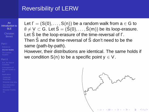
Reversibility of LERW
Let Γ = (S(0), . . . ,S(n)) be a random walk from a ∈ G to∅ 6= V ⊂ G. Let S = (S(0), . . . , S(m)) be its loop-erasure.Let S be the loop-erasure of the time-reversal of Γ.Then S and the time-reversal of S don’t need to be thesame (path-by-path).However, their distributions are identical. The same holds ifwe condition S(n) to be a specific point y ∈ V .
AnIntroduction to
SLE
ChristianBeneš
Part IReferences
Discrete Models
The LoewnerEquation
Part IISLE, the NaturalCandidate
Convergence ofdiscrete models toSLE
Applications
ConformalRestriction
Brownian loop area
Non-intersectionExponents
Brownian Frontier,etc.
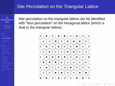
Site Percolation on the Triangular Lattice
Site percolation on the triangular lattice can be identifiedwith “face percolation” on the hexagonal lattice (which isdual to the triangular lattice).
AnIntroduction to
SLE
ChristianBeneš
Part IReferences
Discrete Models
The LoewnerEquation
Part IISLE, the NaturalCandidate
Convergence ofdiscrete models toSLE
Applications
ConformalRestriction
Brownian loop area
Non-intersectionExponents
Brownian Frontier,etc.
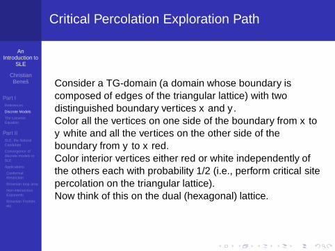
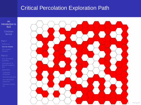
Critical Percolation Exploration Path
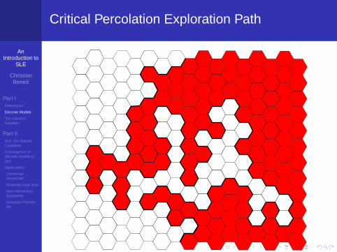
Consider a TG-domain (a domain whose boundary iscomposed of edges of the triangular lattice) with twodistinguished boundary vertices x and y .Color all the vertices on one side of the boundary from x toy white and all the vertices on the other side of theboundary from y to x red.Color interior vertices either red or white independently ofthe others each with probability 1/2 (i.e., perform critical sitepercolation on the triangular lattice).Now think of this on the dual (hexagonal) lattice.
AnIntroduction to
SLE
ChristianBeneš
Part IReferences
Discrete Models
The LoewnerEquation
Part IISLE, the NaturalCandidate
Convergence ofdiscrete models toSLE
Applications
ConformalRestriction
Brownian loop area
Non-intersectionExponents
Brownian Frontier,etc.
Critical Percolation Exploration Path
AnIntroduction to
SLE
ChristianBeneš
Part IReferences
Discrete Models
The LoewnerEquation
Part IISLE, the NaturalCandidate
Convergence ofdiscrete models toSLE
Applications
ConformalRestriction
Brownian loop area
Non-intersectionExponents
Brownian Frontier,etc.
Critical Percolation Exploration Path
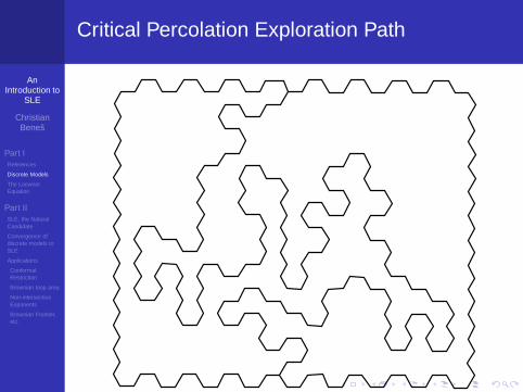
There will be an interface going from x to y whichseparating the red cluster from the white cluster.One way is to draw the interface always keeping a redhexagon on the right and a white hexagon on the left.Another way to visualize the interface is to swallow anyislands so that the domain is partitioned into two connectedsets.
AnIntroduction to
SLE
ChristianBeneš
Part IReferences
Discrete Models
The LoewnerEquation
Part IISLE, the NaturalCandidate
Convergence ofdiscrete models toSLE
Applications
ConformalRestriction
Brownian loop area
Non-intersectionExponents
Brownian Frontier,etc.
Critical Percolation Exploration Path
AnIntroduction to
SLE
ChristianBeneš
Part IReferences
Discrete Models
The LoewnerEquation
Part IISLE, the NaturalCandidate
Convergence ofdiscrete models toSLE
Applications
ConformalRestriction
Brownian loop area
Non-intersectionExponents
Brownian Frontier,etc.
Critical Percolation Exploration Path
AnIntroduction to
SLE
ChristianBeneš
Part IReferences
Discrete Models
The LoewnerEquation
Part IISLE, the NaturalCandidate
Convergence ofdiscrete models toSLE
Applications
ConformalRestriction
Brownian loop area
Non-intersectionExponents
Brownian Frontier,etc.
Discrete Gaussian Free Field
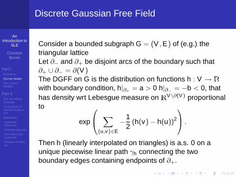
Consider a bounded subgraph G = (V ,E) of (e.g.) thetriangular latticeLet ∂− and ∂+ be disjoint arcs of the boundary such that∂+ ∪ ∂− = ∂(V )The DGFF on G is the distribution on functions h : V → Rwith boundary condition, h|∂+ = a > 0 h|∂
−
= −b < 0, thathas density wrt Lebesgue measure on RV\∂(V ) proportionalto
exp
∑
u,v∈E
−12
(h(v) − h(u))2
.
Then h (linearly interpolated on triangles) is a.s. 0 on aunique piecewise linear path γh connecting the twoboundary edges containing endpoints of ∂+.
AnIntroduction to
SLE
ChristianBeneš
Part IReferences
Discrete Models
The LoewnerEquation
Part IISLE, the NaturalCandidate
Convergence ofdiscrete models toSLE
Applications
ConformalRestriction
Brownian loop area
Non-intersectionExponents
Brownian Frontier,etc.
Discrete Gaussian Free Field
http://tcsmath.files.wordpress.com/2010/12/gff.http://math.nyu.edu/~sheff/sle.html
AnIntroduction to
SLE
ChristianBeneš
Part IReferences
Discrete Models
The LoewnerEquation
Part IISLE, the NaturalCandidate
Convergence ofdiscrete models toSLE
Applications
ConformalRestriction
Brownian loop area
Non-intersectionExponents
Brownian Frontier,etc.
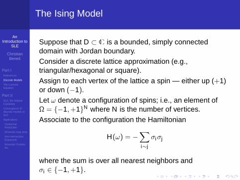
The Ising Model
Suppose that D ⊂ C is a bounded, simply connecteddomain with Jordan boundary.Consider a discrete lattice approximation (e.g.,triangular/hexagonal or square).Assign to each vertex of the lattice a spin — either up (+1)or down (−1).Let ω denote a configuration of spins; i.e., an element ofΩ = −1,+1N where N is the number of vertices.Associate to the configuration the Hamiltonian
H(ω) = −∑
i∼j
σiσj
where the sum is over all nearest neighbors andσi ∈ −1,+1.
AnIntroduction to
SLE
ChristianBeneš
Part IReferences
Discrete Models
The LoewnerEquation
Part IISLE, the NaturalCandidate
Convergence ofdiscrete models toSLE
Applications
ConformalRestriction
Brownian loop area
Non-intersectionExponents
Brownian Frontier,etc.
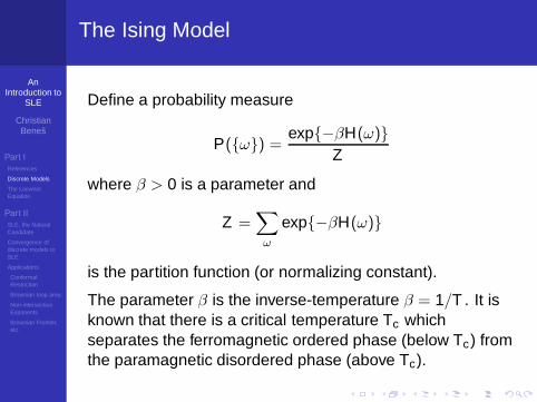
The Ising Model
Define a probability measure
P(ω) =exp−βH(ω)
Z
where β > 0 is a parameter and
Z =∑
ω
exp−βH(ω)
is the partition function (or normalizing constant).
The parameter β is the inverse-temperature β = 1/T . It isknown that there is a critical temperature Tc whichseparates the ferromagnetic ordered phase (below Tc) fromthe paramagnetic disordered phase (above Tc).

AnIntroduction to
SLE
ChristianBeneš
Part IReferences
Discrete Models
The LoewnerEquation
Part IISLE, the NaturalCandidate
Convergence ofdiscrete models toSLE
Applications
ConformalRestriction
Brownian loop area
Non-intersectionExponents
Brownian Frontier,etc.
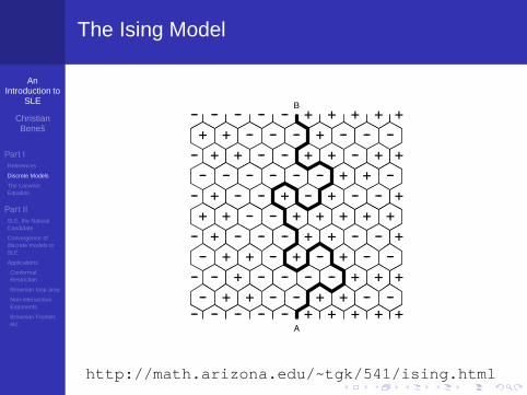
The Ising Model
Fix two arcs on the boundary of the domain and hold oneboundary arc all at spin up and the other all at spin down.
P(ω) now induces a probability measure on curves(interfaces) connecting the two boundary points where theboundary conditions change.
AnIntroduction to
SLE
ChristianBeneš
Part IReferences
Discrete Models
The LoewnerEquation
Part IISLE, the NaturalCandidate
Convergence ofdiscrete models toSLE
Applications
ConformalRestriction
Brownian loop area
Non-intersectionExponents
Brownian Frontier,etc.
The Ising Model
+ + -- -- -- + -- -- --
-- -- -- -- -- + + + + +
-- -- -- -- -- -- + + --
-- + + -- -- + + -- + +
+ + -- -- + + + + +
-- + -- -- + -- + -- -- +
-- + + -- + -- + -- --
-- + -- -- -- + + -- -- +
-- + + -- -- + + -- --
-- -- + -- -- -- -- + + +
-- -- -- -- -- + + + + +
B
A
http://math.arizona.edu/~tgk/541/ising.html
AnIntroduction to
SLE
ChristianBeneš
Part IReferences
Discrete Models
The LoewnerEquation
Part IISLE, the NaturalCandidate
Convergence ofdiscrete models toSLE
Applications
ConformalRestriction
Brownian loop area
Non-intersectionExponents
Brownian Frontier,etc.
Uniform Spanning Tree and Peano Curve
http://stat.math.uregina.ca/~kozdron/Simulation
AnIntroduction to
SLE
ChristianBeneš
Part IReferences
Discrete Models
The LoewnerEquation
Part IISLE, the NaturalCandidate
Convergence ofdiscrete models toSLE
Applications
ConformalRestriction
Brownian loop area
Non-intersectionExponents
Brownian Frontier,etc.
Domain Markov Property
So what should the scaling limit of such processes looklike? These models are clearly not Markovian. However, asit turns out, they all satisfy a type of Markov property.Let D be a grid domain (where the boundary is composed ofedges of Z2) and ∅ 6= V ( D and let x ∈ D, y ∈ V .Let L(x , y ; V ) be the law of the loop-erasure of SRW Sconditioned on the event that S hits V at y . Then the law ofS[0, σ − j] given thatS(σ − j) = yj , S(σ − (j − 1)) = yj−1), . . . , S(σ) = y0(assuming that this event is possible) isL(x , yj ; V ∪ y0, y1, . . . , yj).
AnIntroduction to
SLE
ChristianBeneš
Part IReferences
Discrete Models
The LoewnerEquation
Part IISLE, the NaturalCandidate
Convergence ofdiscrete models toSLE
Applications
ConformalRestriction
Brownian loop area
Non-intersectionExponents
Brownian Frontier,etc.
Domain Markov Property
For the processes that arise as interfaces, the Markovproperty requires adapting the boundary condition. Themodel in which this property is most obvious is the criticalpercolation interface:Let L(x , y) be the law of the critical percolation interface γfrom x to y inD with boundary condition “on" for verticestraversed clockwise from x to y and “off" for the others.Then the law of γ[σ − j , σ] given thatγ(0) = x , γ(1) = y1, . . . , γ(σ − j) = yσ−j (assuming thatthis event is possible) is the same as the law of the criticalpercolation interface γ from yσ−j to y inD ∪ y0, y1, . . . yσ−j.
AnIntroduction to
SLE
ChristianBeneš
Part IReferences
Discrete Models
The LoewnerEquation
Part IISLE, the NaturalCandidate
Convergence ofdiscrete models toSLE
Applications
ConformalRestriction
Brownian loop area
Non-intersectionExponents
Brownian Frontier,etc.
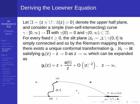
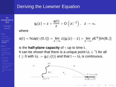
Deriving the Loewner Equation
Let H = z ∈ C : ℑ(z) > 0 denote the upper half plane,and consider a simple (non-self-intersecting) curveγ : [0,∞) → H with γ(0) = 0 and γ(0,∞) ⊂ H.For every fixed t ≥ 0, the slit plane Ht := H \ γ(0, t] issimply connected and so by the Riemann mapping theorem,there exists a unique conformal transformation gt : Ht → Hsatisfying gt(z) − z → 0 as z → ∞ which can be expandedas
gt(z) = z +a(t)
z+ O
(
|z|−2)
, z → ∞,
H t H (0) = 0 Ut := gt( (t))gt [0; t ! (t)
gt( [0; t) R
AnIntroduction to
SLE
ChristianBeneš
Part IReferences
Discrete Models
The LoewnerEquation
Part IISLE, the NaturalCandidate
Convergence ofdiscrete models toSLE
Applications
ConformalRestriction
Brownian loop area
Non-intersectionExponents
Brownian Frontier,etc.
Deriving the Loewner Equation
gt(z) = z +a(t)
z+ O
(
|z|−2)
, z → ∞,
where
a(t) = hcap(γ(0, t]) = limz→∞
z(gt (z) − z) = limy→∞
yE iy [Im(Bτ )]
is the half-plane capacity of γ up to time t .It can be shown that there is a unique point Ut ∈ R for allt ≥ 0 with Ut := gt(γ(t)) and that t 7→ Ut is continuous.H t H
(0) = 0 Ut := gt( (t))gt [0; t ! (t)gt( [0; t) R
AnIntroduction to
SLE
ChristianBeneš
Part IReferences
Discrete Models
The LoewnerEquation
Part IISLE, the NaturalCandidate
Convergence ofdiscrete models toSLE
Applications
ConformalRestriction
Brownian loop area
Non-intersectionExponents
Brownian Frontier,etc.
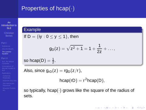
Properties of hcap(·)
Example
If D = iy : 0 ≤ y ≤ 1, then
gD(z) =√
z2 + 1 = 1 +1
2z+ . . . ,
so hcap(D) = 12 .
Also, since grD(z) = rgD(z/r),
hcap(rD) = r2hcap(D),
so typically, hcap(·) grows like the square of the radius ofsets.
AnIntroduction to
SLE
ChristianBeneš
Part IReferences
Discrete Models
The LoewnerEquation
Part IISLE, the NaturalCandidate
Convergence ofdiscrete models toSLE
Applications
ConformalRestriction
Brownian loop area
Non-intersectionExponents
Brownian Frontier,etc.
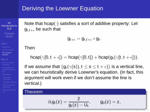
Deriving the Loewner Equation
Note that hcap(·) satisfies a sort of additive property: Letgt,t+ǫ be such that
gt+ǫ = gt,t+ǫ gt .
Then
hcap(γ[0, t + ǫ]) = hcap(γ[0, t]) + hcap(gt(γ[t , t + ǫ])).
If we assume that gt(γ(s)), t ≤ s ≤ t + ǫ) is a vertical line,we can heuristically derive Loewner’s equation. (In fact, thisargument will work even if we don’t assume the line isvertical.)
Theorem
∂tgt(z) =2
gt(z) − Ut, g0(z) = z,
AnIntroduction to
SLE
ChristianBeneš
Part IReferences
Discrete Models
The LoewnerEquation
Part IISLE, the NaturalCandidate
Convergence ofdiscrete models toSLE
Applications
ConformalRestriction
Brownian loop area
Non-intersectionExponents
Brownian Frontier,etc.
The Loewner Equation as a flow
We can fix z and look at its evolution in time via theLoewner ODE:
gt(z) − Ut = xt(z) + iyt(z)
with xt(z) ∈ R and yt(z) ∈ R+. So
∂tgt(z) =2
gt(z) − Ut=
xt(z) − iyt(z)
x2t (z) + y2
t (z),
which has negative imaginary part. So gt(z)t≥0 is adownward flow (until gt(z) = Ut at which point z is hit by thecurve γ).
AnIntroduction to
SLE
ChristianBeneš
Part IReferences
Discrete Models
The LoewnerEquation
Part IISLE, the NaturalCandidate
Convergence ofdiscrete models toSLE
Applications
ConformalRestriction
Brownian loop area
Non-intersectionExponents
Brownian Frontier,etc.
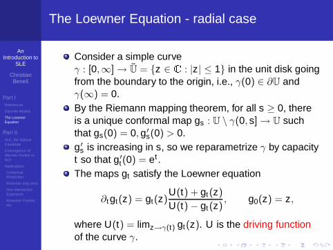
The Loewner Equation - radial case
Consider a simple curveγ : [0,∞] → U = z ∈ C : |z| ≤ 1 in the unit disk goingfrom the boundary to the origin, i.e., γ(0) ∈ ∂U andγ(∞) = 0.By the Riemann mapping theorem, for all s ≥ 0, thereis a unique conformal map gs : U \ γ(0, s] → U suchthat gs(0) = 0,g′
s(0) > 0.g′
s is increasing in s, so we reparametrize γ by capacityt so that g′
t(0) = et .The maps gt satisfy the Loewner equation
∂tgt(z) = gt(z)U(t) + gt(z)
U(t) − gt(z), g0(z) = z,
where U(t) = limz→γ(t) gt(z). U is the driving functionof the curve γ.
AnIntroduction to
SLE
ChristianBeneš
Part IReferences
Discrete Models
The LoewnerEquation
Part IISLE, the NaturalCandidate
Convergence ofdiscrete models toSLE
Applications
ConformalRestriction
Brownian loop area
Non-intersectionExponents
Brownian Frontier,etc.
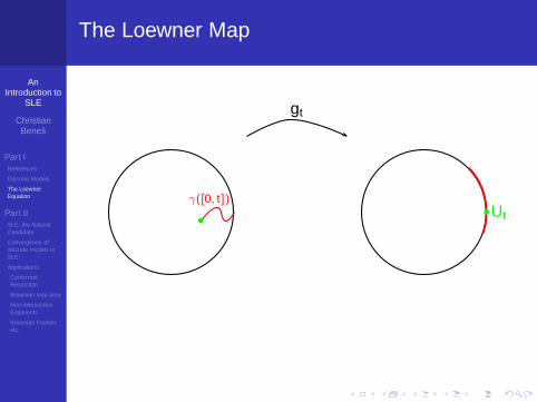
The Loewner Map
gt
bb
γ([0, t])Ut
AnIntroduction to
SLE
ChristianBeneš
Part IReferences
Discrete Models
The LoewnerEquation
Part IISLE, the NaturalCandidate
Convergence ofdiscrete models toSLE
Applications
ConformalRestriction
Brownian loop area
Non-intersectionExponents
Brownian Frontier,etc.
The Loewner Equation - radial case
Just as one can obtain U from γ, one can go backwards viaLoewner’s equation and start with the driving function U andobtain a sequence of maps gt from it. This will yield anassociated curve γ if U is Hölder-1/2.
AnIntroduction to
SLE
ChristianBeneš
Part IReferences
Discrete Models
The LoewnerEquation
Part IISLE, the NaturalCandidate
Convergence ofdiscrete models toSLE
Applications
ConformalRestriction
Brownian loop area
Non-intersectionExponents
Brownian Frontier,etc.
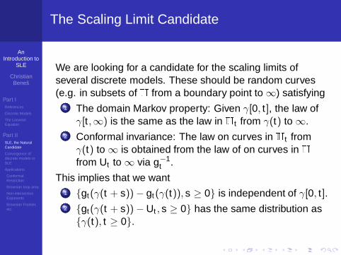
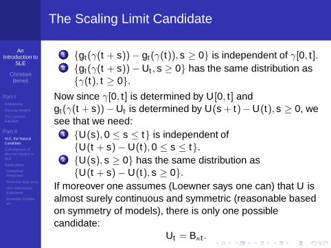
The Scaling Limit Candidate
We are looking for a candidate for the scaling limits ofseveral discrete models. These should be random curves(e.g. in subsets of H from a boundary point to ∞) satisfying
1 The domain Markov property: Given γ[0, t], the law ofγ[t ,∞) is the same as the law in Ht from γ(t) to ∞.
2 Conformal invariance: The law on curves in Ht fromγ(t) to ∞ is obtained from the law of on curves in Hfrom Ut to ∞ via g−1
t .
This implies that we want1 gt(γ(t + s)) − gt(γ(t)), s ≥ 0 is independent of γ[0, t].2 gt(γ(t + s)) − Ut , s ≥ 0 has the same distribution as
γ(t), t ≥ 0.
AnIntroduction to
SLE
ChristianBeneš
Part IReferences
Discrete Models
The LoewnerEquation
Part IISLE, the NaturalCandidate
Convergence ofdiscrete models toSLE
Applications
ConformalRestriction
Brownian loop area
Non-intersectionExponents
Brownian Frontier,etc.
The Scaling Limit Candidate
1 gt(γ(t + s)) − gt(γ(t)), s ≥ 0 is independent of γ[0, t].2 gt(γ(t + s)) − Ut , s ≥ 0 has the same distribution as
γ(t), t ≥ 0.
Now since γ[0, t] is determined by U[0, t] andgt(γ(t + s))− Ut is determined by U(s + t)−U(t), s ≥ 0, wesee that we need:
1 U(s),0 ≤ s ≤ t is independent ofU(t + s) − U(t),0 ≤ s ≤ t.
2 U(s), s ≥ 0 has the same distribution asU(t + s) − U(t), s ≥ 0.
If moreover one assumes (Loewner says one can) that U isalmost surely continuous and symmetric (reasonable basedon symmetry of models), there is only one possiblecandidate:
Ut = Bκt .
AnIntroduction to
SLE
ChristianBeneš
Part IReferences
Discrete Models
The LoewnerEquation
Part IISLE, the NaturalCandidate
Convergence ofdiscrete models toSLE
Applications
ConformalRestriction
Brownian loop area
Non-intersectionExponents
Brownian Frontier,etc.
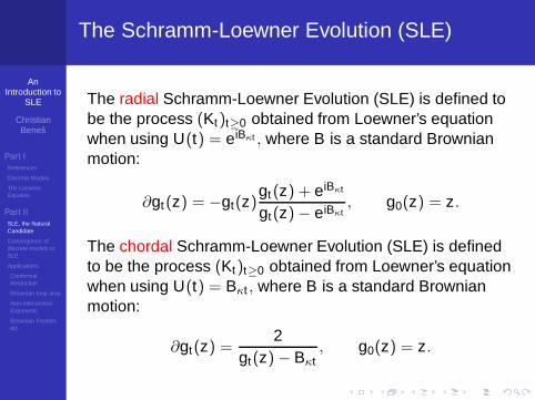
The Schramm-Loewner Evolution (SLE)
The radial Schramm-Loewner Evolution (SLE) is defined tobe the process (Kt)t≥0 obtained from Loewner’s equationwhen using U(t) = eiBκt , where B is a standard Brownianmotion:
∂gt(z) = −gt(z)gt (z) + eiBκt
gt(z) − eiBκt, g0(z) = z.
The chordal Schramm-Loewner Evolution (SLE) is definedto be the process (Kt)t≥0 obtained from Loewner’s equationwhen using U(t) = Bκt , where B is a standard Brownianmotion:
∂gt(z) =2
gt(z) − Bκt, g0(z) = z.
AnIntroduction to
SLE
ChristianBeneš
Part IReferences
Discrete Models
The LoewnerEquation
Part IISLE, the NaturalCandidate
Convergence ofdiscrete models toSLE
Applications
ConformalRestriction
Brownian loop area
Non-intersectionExponents
Brownian Frontier,etc.
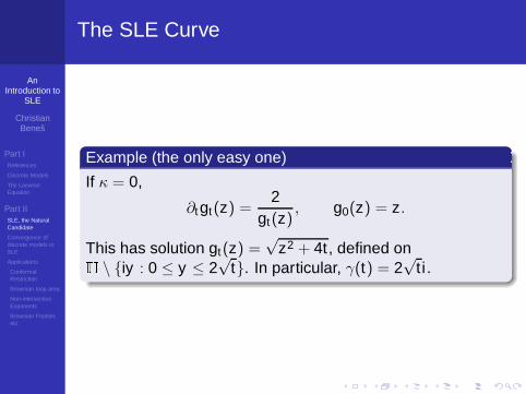
The SLE Curve
Example (the only easy one)
If κ = 0,
∂tgt(z) =2
gt(z), g0(z) = z.
This has solution gt(z) =√
z2 + 4t , defined onH \ iy : 0 ≤ y ≤ 2√
t. In particular, γ(t) = 2√
t i .
AnIntroduction to
SLE
ChristianBeneš
Part IReferences
Discrete Models
The LoewnerEquation
Part IISLE, the NaturalCandidate
Convergence ofdiscrete models toSLE
Applications
ConformalRestriction
Brownian loop area
Non-intersectionExponents
Brownian Frontier,etc.
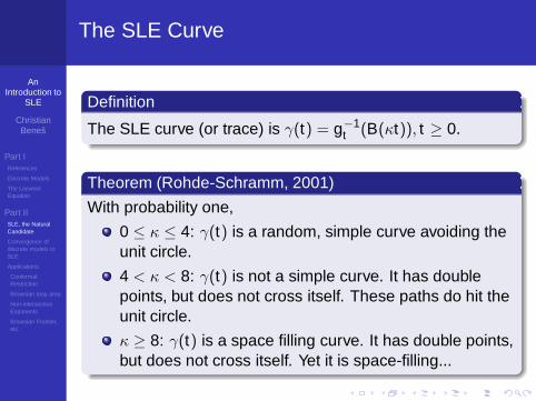
The SLE Curve
Definition
The SLE curve (or trace) is γ(t) = g−1t (B(κt)), t ≥ 0.
Theorem (Rohde-Schramm, 2001)
With probability one,
0 ≤ κ ≤ 4: γ(t) is a random, simple curve avoiding theunit circle.
4 < κ < 8: γ(t) is not a simple curve. It has doublepoints, but does not cross itself. These paths do hit theunit circle.
κ ≥ 8: γ(t) is a space filling curve. It has double points,but does not cross itself. Yet it is space-filling...
AnIntroduction to
SLE
ChristianBeneš
Part IReferences
Discrete Models
The LoewnerEquation
Part IISLE, the NaturalCandidate
Convergence ofdiscrete models toSLE
Applications
ConformalRestriction
Brownian loop area
Non-intersectionExponents
Brownian Frontier,etc.
The SLE Curve
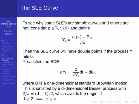
To see why some SLE’s are simple curves and others arenot, consider z ∈ R \ 0 and define
Yt =gt(z) − Bκt√
κ.
Then the SLE curve will have double points if the process Yt
hits 0.Y satisfies the SDE
dYt =2κYt
dt − dBt ,
where B is a one-dimensional standard Brownian motion.This is satisfied by a d -dimensional Bessel process with2/κ = (d − 1)/2, which avoids the origin iffd ≥ 2 ⇐⇒ κ ≤ 4.
AnIntroduction to
SLE
ChristianBeneš
Part IReferences
Discrete Models
The LoewnerEquation
Part IISLE, the NaturalCandidate
Convergence ofdiscrete models toSLE
Applications
ConformalRestriction
Brownian loop area
Non-intersectionExponents
Brownian Frontier,etc.
The SLE Curve
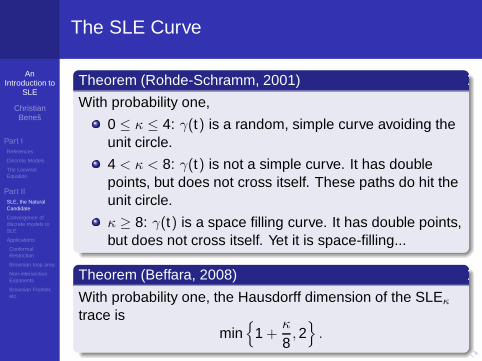
Theorem (Rohde-Schramm, 2001)
With probability one,
0 ≤ κ ≤ 4: γ(t) is a random, simple curve avoiding theunit circle.
4 < κ < 8: γ(t) is not a simple curve. It has doublepoints, but does not cross itself. These paths do hit theunit circle.
κ ≥ 8: γ(t) is a space filling curve. It has double points,but does not cross itself. Yet it is space-filling...
Theorem (Beffara, 2008)
With probability one, the Hausdorff dimension of the SLEκ
trace ismin
1 +κ
8,2
.
AnIntroduction to
SLE
ChristianBeneš
Part IReferences
Discrete Models
The LoewnerEquation
Part IISLE, the NaturalCandidate
Convergence ofdiscrete models toSLE
Applications
ConformalRestriction
Brownian loop area
Non-intersectionExponents
Brownian Frontier,etc.
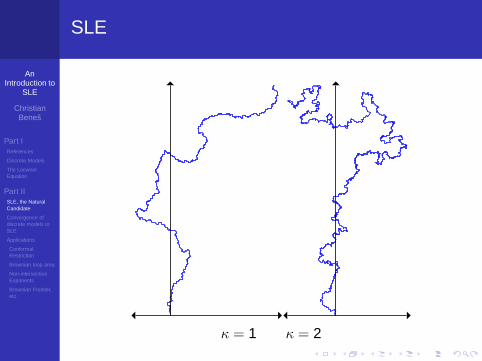
SLE
κ = 1 κ = 2
AnIntroduction to
SLE
ChristianBeneš
Part IReferences
Discrete Models
The LoewnerEquation
Part IISLE, the NaturalCandidate
Convergence ofdiscrete models toSLE
Applications
ConformalRestriction
Brownian loop area
Non-intersectionExponents
Brownian Frontier,etc.
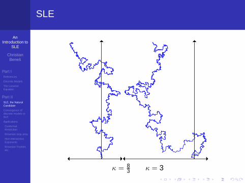
SLE
κ = 83 κ = 3
AnIntroduction to
SLE
ChristianBeneš
Part IReferences
Discrete Models
The LoewnerEquation
Part IISLE, the NaturalCandidate
Convergence ofdiscrete models toSLE
Applications
ConformalRestriction
Brownian loop area
Non-intersectionExponents
Brownian Frontier,etc.
Other SLE’s
In general simply connected domains D, we can defineradial SLE from w ∈ ∂D to z ∈ D as the conformal image ofradial SLE in the unit disk under the map ψ : U 7→ D withψ(1) = w and ψ(0) = z.
Similarly, via conformal mapping, one can define chordalSLE in simply connected domains D going from w ∈ ∂D toz ∈ ∂D.
AnIntroduction to
SLE
ChristianBeneš
Part IReferences
Discrete Models
The LoewnerEquation
Part IISLE, the NaturalCandidate
Convergence ofdiscrete models toSLE
Applications
ConformalRestriction
Brownian loop area
Non-intersectionExponents
Brownian Frontier,etc.
SLE’s successes (and one big open problem)
Application to planar Brownian motion:
dimH(frontier) = 4/3, dimH(cutpoints) = 3/4.(LSW )
SLE2 is the scaling limit of LERW. (Lawler, Schramm,Werner)SLE3 is the scaling limit of the critical Ising modelinterface. (Smirnov)SLE4 is the scaling limit of the harmonic explorer andthe discrete Gaussian free field interface. (Schramm,Sheffield)SLE6 is the scaling limit of the critical percolationexploration path on the triangular lattice. (Smirnov)SLE8 is the scaling limit of the uniform spanning treePeano curve. (LSW)SLE8/3 is conjectured to be the scaling limit of theself-avoiding walk.
AnIntroduction to
SLE
ChristianBeneš
Part IReferences
Discrete Models
The LoewnerEquation
Part IISLE, the NaturalCandidate
Convergence ofdiscrete models toSLE
Applications
ConformalRestriction
Brownian loop area
Non-intersectionExponents
Brownian Frontier,etc.
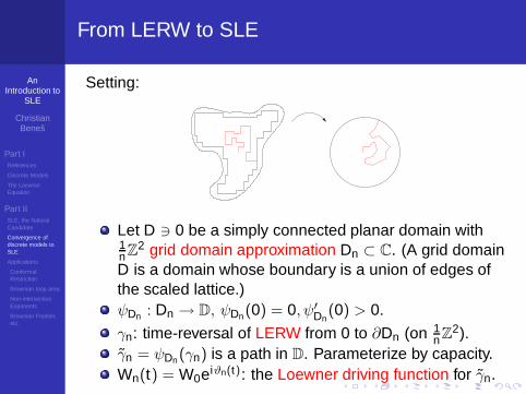
From LERW to SLE
Setting:
Let D ∋ 0 be a simply connected planar domain with1nZ2 grid domain approximation Dn ⊂ C. (A grid domainD is a domain whose boundary is a union of edges ofthe scaled lattice.)ψDn : Dn → D, ψDn(0) = 0, ψ′
Dn(0) > 0.
γn: time-reversal of LERW from 0 to ∂Dn (on 1nZ2).
γn = ψDn(γn) is a path in D. Parameterize by capacity.Wn(t) = W0eiϑn(t): the Loewner driving function for γn.
AnIntroduction to
SLE
ChristianBeneš
Part IReferences
Discrete Models
The LoewnerEquation
Part IISLE, the NaturalCandidate
Convergence ofdiscrete models toSLE
Applications
ConformalRestriction
Brownian loop area
Non-intersectionExponents
Brownian Frontier,etc.
LSW’s result
A weak form of the convergence result is the following:
Theorem (Lawler, Schramm, Werner, 2004)
Let D be the set of simply connected grid domains with0 ∈ D,D 6= C. For every T > 0, ǫ > 0, there existsn = n(T , ǫ) such that if D ∈ D with inrad(D) > n, then thereexists a coupling between loop-erased random walk γ from∂D to 0 in D and Brownian motion B started uniformly on[0,2π] such that
P(sup|θ(t) − B(2t)| : t ∈ [0,T ] > ǫ < ǫ,
where θ(t) satisfies W (t) = W (0)eiθ(t) and W (t) is thedriving process of γ in Loewner’s equation.
This result leads to the stronger convergence of paths withrespect to Hausdorff metric.
AnIntroduction to
SLE
ChristianBeneš
Part IReferences
Discrete Models
The LoewnerEquation
Part IISLE, the NaturalCandidate
Convergence ofdiscrete models toSLE
Applications
ConformalRestriction
Brownian loop area
Non-intersectionExponents
Brownian Frontier,etc.
Ideas of Proof
Three main steps
1 Find a discrete martingale observable for the LERWpath. Prove that it converges to something conformallyinvariant.
2 Use Step 1 together with the Loewner equation to showthat the Loewner driving function is almost a martingalewith “correct” (conditional) variance.
3 Use Step 2 and Skorokhod embedding to couple theLoewner driving function with a Brownian motion andshow that they are uniformly close with high probability.
AnIntroduction to
SLE
ChristianBeneš
Part IReferences
Discrete Models
The LoewnerEquation
Part IISLE, the NaturalCandidate
Convergence ofdiscrete models toSLE
Applications
ConformalRestriction
Brownian loop area
Non-intersectionExponents
Brownian Frontier,etc.
A Rate for the Driving Function
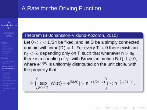
Theorem (B-Johansson-Viklund-Kozdron, 2010)
Let 0 < ǫ < 1/24 be fixed, and let D be a simply connecteddomain with inrad(D) = 1. For every T > 0 there exists ann0 <∞ depending only on T such that whenever n > n0
there is a coupling of γn with Brownian motion B(t), t ≥ 0,where eiB(0) is uniformly distributed on the unit circle, withthe property that
P
(
sup0≤t≤T
|Wn(t) − eiB(2t)| > n−(1/24−ǫ)
)
< n−(1/24−ǫ).
AnIntroduction to
SLE
ChristianBeneš
Part IReferences
Discrete Models
The LoewnerEquation
Part IISLE, the NaturalCandidate
Convergence ofdiscrete models toSLE
Applications
ConformalRestriction
Brownian loop area
Non-intersectionExponents
Brownian Frontier,etc.
A Rate for the Processes
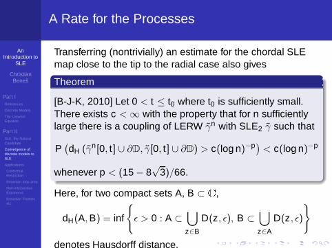
Transferring (nontrivially) an estimate for the chordal SLEmap close to the tip to the radial case also gives
Theorem
[B-J-K, 2010] Let 0 < t ≤ t0 where t0 is sufficiently small.There exists c <∞ with the property that for n sufficientlylarge there is a coupling of LERW γn with SLE2 γ such that
P(
dH (γn[0, t] ∪ ∂D, γ[0, t] ∪ ∂D) > c(log n)−p) < c(log n)−p
whenever p < (15 − 8√
3)/66.
Here, for two compact sets A, B ⊂ C,
dH(A,B) = inf
ǫ > 0 : A ⊂⋃
z∈B
D(z, ǫ), B ⊂⋃
z∈A
D(z, ǫ)
denotes Hausdorff distance.
AnIntroduction to
SLE
ChristianBeneš
Part IReferences
Discrete Models
The LoewnerEquation
Part IISLE, the NaturalCandidate
Convergence ofdiscrete models toSLE
Applications
ConformalRestriction
Brownian loop area
Non-intersectionExponents
Brownian Frontier,etc.
Applications of rate?
P(
dH (γn[0, t] ∪ ∂D, γ[0, t] ∪ ∂D) > c(log n)−p) < c(log n)−p
In the same way that KMT and Skorokhod embedding areinstrumental in transferring results from Brownian motion toSLE, one could hope that this result (and others of the sametype for the other processes known to converge to SLE)could lead to estimates for the discrete models, based oncomputations for SLE.
AnIntroduction to
SLE
ChristianBeneš
Part IReferences
Discrete Models
The LoewnerEquation
Part IISLE, the NaturalCandidate
Convergence ofdiscrete models toSLE
Applications
ConformalRestriction
Brownian loop area
Non-intersectionExponents
Brownian Frontier,etc.
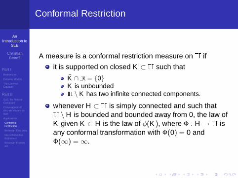
Conformal Restriction
A measure is a conformal restriction measure on H if
it is supported on closed K ⊂ H such that
K ∩R = 0K is unboundedH \ K has two infinite connected components.
whenever H ⊂ H is simply connected and such thatH \ H is bounded and bounded away from 0, the law ofK given K ⊂ H is the law of φ(K ), where Φ : H → H isany conformal transformation with Φ(0) = 0 andΦ(∞) = ∞.
AnIntroduction to
SLE
ChristianBeneš
Part IReferences
Discrete Models
The LoewnerEquation
Part IISLE, the NaturalCandidate
Convergence ofdiscrete models toSLE
Applications
ConformalRestriction
Brownian loop area
Non-intersectionExponents
Brownian Frontier,etc.
Conformal Restriction
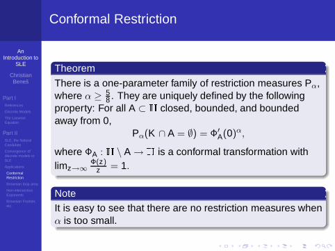
Theorem
There is a one-parameter family of restriction measures Pα,where α ≥ 5
8 . They are uniquely defined by the followingproperty: For all A ⊂ H closed, bounded, and boundedaway from 0,
Pα(K ∩ A = ∅) = Φ′A(0)α,
where ΦA : H \ A → H is a conformal transformation withlimz→∞
Φ(z)z = 1.
NoteIt is easy to see that there are no restriction measures whenα is too small.
AnIntroduction to
SLE
ChristianBeneš
Part IReferences
Discrete Models
The LoewnerEquation
Part IISLE, the NaturalCandidate
Convergence ofdiscrete models toSLE
Applications
ConformalRestriction
Brownian loop area
Non-intersectionExponents
Brownian Frontier,etc.
Conformal Restriction Examples
Example
SLE8/3 has law P5/8.
Example
Brownian Excursion has law P1.
AnIntroduction to
SLE
ChristianBeneš
Part IReferences
Discrete Models
The LoewnerEquation
Part IISLE, the NaturalCandidate
Convergence ofdiscrete models toSLE
Applications
ConformalRestriction
Brownian loop area
Non-intersectionExponents
Brownian Frontier,etc.
Conformal Restriction Additive Property
Definition
For K ⊂ H such that K ∩R = 0,K is unbounded, andH \ K has two infinite connected components, let F(K ), thefilling of K be the set of points in H \ K that are not in theconnected components that have (0,∞) and (−∞,0) intheir boundaries.
Let F(Fi), i = 1, . . . , k satisfy conformal restriction withexponent αi . Then F(∪n
i=1Fi) satisfies conformal restrictionwith exponent
∑ni=1 αi .
A consequence is that the hull of 8 SLE8/3 paths and thehull of 5 Brownian motions are the same.
AnIntroduction to
SLE
ChristianBeneš
Part IReferences
Discrete Models
The LoewnerEquation
Part IISLE, the NaturalCandidate
Convergence ofdiscrete models toSLE
Applications
ConformalRestriction
Brownian loop area
Non-intersectionExponents
Brownian Frontier,etc.
Area of Filled Planar Brownian Loop
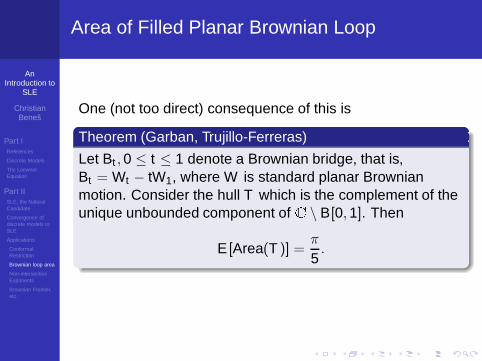
One (not too direct) consequence of this is
Theorem (Garban, Trujillo-Ferreras)
Let Bt ,0 ≤ t ≤ 1 denote a Brownian bridge, that is,Bt = Wt − tW1, where W is standard planar Brownianmotion. Consider the hull T which is the complement of theunique unbounded component of C \ B[0,1]. Then
E [Area(T )] =π
5.
AnIntroduction to
SLE
ChristianBeneš
Part IReferences
Discrete Models
The LoewnerEquation
Part IISLE, the NaturalCandidate
Convergence ofdiscrete models toSLE
Applications
ConformalRestriction
Brownian loop area
Non-intersectionExponents
Brownian Frontier,etc.
Area of Filled Planar Brownian Loop
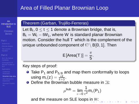
Theorem (Garban, Trujillo-Ferreras)
Let Bt ,0 ≤ t ≤ 1 denote a Brownian bridge, that is,Bt = Wt − tW1, where W is standard planar Brownianmotion. Consider the hull T which is the complement of theunique unbounded component of C \ B[0,1]. Then
E [Area(T )] =π
5.
Key steps of proof:
Take P1 and P5/8 and map them conformally to loopsusing mǫ(z) = ǫz
z+1 .Define the Brownian bubble measure in H:
µbub = limǫ→0
1ǫ2
mǫ(P1)
and the measure on SLE loops in H:
1

AnIntroduction to
SLE
ChristianBeneš
Part IReferences
Discrete Models
The LoewnerEquation
Part IISLE, the NaturalCandidate
Convergence ofdiscrete models toSLE
Applications
ConformalRestriction
Brownian loop area
Non-intersectionExponents
Brownian Frontier,etc.
Area of Filled Planar Brownian Loop
Key steps of proof:
Take P1 and P5/8 and map them conformally to loopsusing mǫ(z) = ǫz
z+1 .
Define the Brownian bubble measure in H:
µbub = limǫ→0
1ǫ2
mǫ(P1)
and the measure on SLE loops in H:
µsle = limǫ→0
1ǫ2
mǫ(P5/8).
Note that µsle = 58µ
bub = 58
∫∞0
dt2t2 Pbr
t × Pexct . Here, Pbr
tand Pexc
t are the laws of a 1-d Brownian bridge and a1-d Brownian excursion, respectively, of time duration t .
AnIntroduction to
SLE
ChristianBeneš
Part IReferences
Discrete Models
The LoewnerEquation
Part IISLE, the NaturalCandidate
Convergence ofdiscrete models toSLE
Applications
ConformalRestriction
Brownian loop area
Non-intersectionExponents
Brownian Frontier,etc.
Area of Filled Planar Brownian Loop
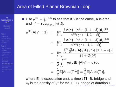
Use µsle = 58µ
bub to see that if γ is the curve, A is area,and γ∗ = sup0≤t≤1 |γ(t)|,
µsle(A|γ∗ = 1) = limδ→0
∫
A(γ)1γ∗ ∈ [1,1 + δ)dµsle
µsle(γ∗ ∈ [1,1 + δ))
= limδ→0
∫
A(γ)1γ∗ ∈ [1,1 + δ)dµbub
µbub(γ∗ ∈ [1,1 + δ))
= limδ→0
∫∞0
dt2t2 Et [A(γ)1γ∗ ∈ [1,1 + δ)]
2δ + O(δ2)
=12
∫ ∞
0η1(u)E1[A|γ∗ = u) du
=12
E [Area(TH)] =12
E [Area(T )],
where Et is expectation w.r.t. a time t H−B. bridge andη1 is the density of γ∗ for the H−B. bridge of duration 1.

AnIntroduction to
SLE
ChristianBeneš
Part IReferences
Discrete Models
The LoewnerEquation
Part IISLE, the NaturalCandidate
Convergence ofdiscrete models toSLE
Applications
ConformalRestriction
Brownian loop area
Non-intersectionExponents
Brownian Frontier,etc.
Area of Filled Planar Brownian Loop
We just saw that
E [Area(T )] = 2µsle(A|γ∗ = 1).
We now turn to computing µsle(A|γ∗ = 1) using SLEtechniques. If we write Eǫ for the expected value under thelaw mǫ(P5/8), we have
µsle(A|γ∗ = 1) = limδ→0
limǫ→0
Eǫ[A(γ)|γ∗ ∈ [1,1 + δ)]
=
∫
D∩H limǫ→0
Pǫ(z inside |γ∗ = 1)dA(z)
To compute for a given z0,Pǫ(z0 inside |γ∗ = 1), we canmap back the SLE bubble to chordal SLE8/3 and use therestriction property.
AnIntroduction to
SLE
ChristianBeneš
Part IReferences
Discrete Models
The LoewnerEquation
Part IISLE, the NaturalCandidate
Convergence ofdiscrete models toSLE
Applications
ConformalRestriction
Brownian loop area
Non-intersectionExponents
Brownian Frontier,etc.
Area of Filled Planar Brownian Loop
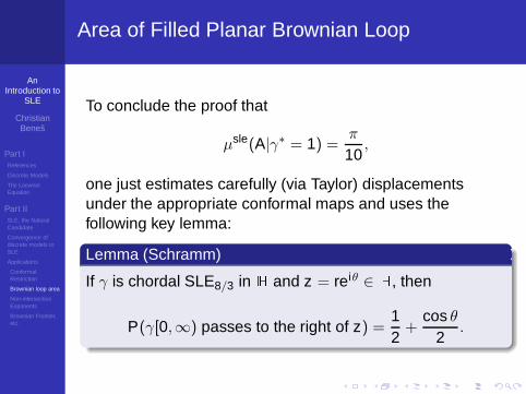
To conclude the proof that
µsle(A|γ∗ = 1) =π
10,
one just estimates carefully (via Taylor) displacementsunder the appropriate conformal maps and uses thefollowing key lemma:
Lemma (Schramm)
If γ is chordal SLE8/3 in H and z = reiθ ∈ H, then
P(γ[0,∞) passes to the right of z) =12
+cos θ
2.
AnIntroduction to
SLE
ChristianBeneš
Part IReferences
Discrete Models
The LoewnerEquation
Part IISLE, the NaturalCandidate
Convergence ofdiscrete models toSLE
Applications
ConformalRestriction
Brownian loop area
Non-intersectionExponents
Brownian Frontier,etc.
Intersection and Disconnection Exponents
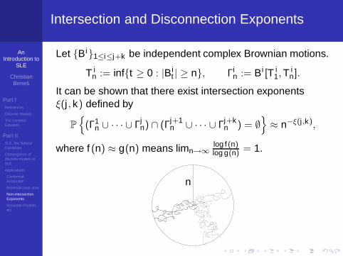
Let Bi1≤i≤j+k be independent complex Brownian motions.
T in := inft ≥ 0 : |Bi
t | ≥ n, Γin := Bi [T i
1,Tin].
It can be shown that there exist intersection exponentsξ(j , k) defined by
P
(Γ1n ∪ · · · ∪ Γj
n) ∩ (Γj+1n ∪ · · · ∪ Γj+k
n ) = ∅
≈ n−ξ(j ,k),
where f (n) ≈ g(n) means limn→∞log f (n)log g(n) = 1.
1
n
AnIntroduction to
SLE
ChristianBeneš
Part IReferences
Discrete Models
The LoewnerEquation
Part IISLE, the NaturalCandidate
Convergence ofdiscrete models toSLE
Applications
ConformalRestriction
Brownian loop area
Non-intersectionExponents
Brownian Frontier,etc.
Intersection and Disconnection Exponents
If Zn = Zn(Γ1n ∪ · · · ∪ Γj
n) :=
P
(Γ1n ∪ · · · ∪ Γj
n) ∩ Γj+1n = ∅|Γ1
n, · · · ,Γjn
, then
E[
Z kn
]
= P
(Γ1n ∪ · · · ∪ Γ
jn) ∩ (Γ
j+1n ∪ · · · ∪ Γ
j+kn ) = ∅
,
soE[
Z kn
]
≈ n−ξ(j ,k).
This leads to a definition of ξ(j , λ) for any λ ∈ R+ (with theconvention 00 = 0), via
E[
Z λn
]
≈ n−ξ(j ,λ).
The disconnection exponent ξ(j ,0) is then defined by
P Zn > 0 ≈ n−ξ(j ,0).
AnIntroduction to
SLE
ChristianBeneš
Part IReferences
Discrete Models
The LoewnerEquation
Part IISLE, the NaturalCandidate
Convergence ofdiscrete models toSLE
Applications
ConformalRestriction
Brownian loop area
Non-intersectionExponents
Brownian Frontier,etc.
Intersection and Disconnection Exponents
The disconnection exponent ξ(j ,0) is then defined by
P Zn > 0 ≈ n−ξ(j ,0).
Equivalently, if
U jn = unbounded component of C \ Γ1
n ∪ · · · ∪ Γjn,
P
U jn ∩ D(0,1) 6= ∅
≈ n−ξ(j ,0).
(ξ(1,0) is called the one-sided disconnection exponent andξ(2,0) the two-sided disconnection exponent.)Burdzy-Lawler (1990) and Lawler-Puckette (1997,2000)showed the equality of the Brownian exponents andanalogously defined random walk exponents.
AnIntroduction to
SLE
ChristianBeneš
Part IReferences
Discrete Models
The LoewnerEquation
Part IISLE, the NaturalCandidate
Convergence ofdiscrete models toSLE
Applications
ConformalRestriction
Brownian loop area
Non-intersectionExponents
Brownian Frontier,etc.
Intersection and Disconnection Exponents
ξ(1,0) is called the one-sided disconnection exponent andξ(2,0) the two-sided disconnection exponent.Lawler, Schramm, and Werner’s work on theSchramm-Loewner Evolution allowed them to find anumerical expression for the intersection and disconnectionexponents. In particular,
Theorem (2001, Lawler-Schramm-Werner)
ξ(1,0) =14
and ξ(2,0) =23.
AnIntroduction to
SLE
ChristianBeneš
Part IReferences
Discrete Models
The LoewnerEquation
Part IISLE, the NaturalCandidate
Convergence ofdiscrete models toSLE
Applications
ConformalRestriction
Brownian loop area
Non-intersectionExponents
Brownian Frontier,etc.
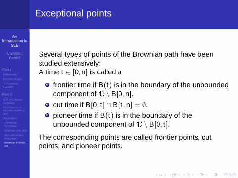
Exceptional points
Several types of points of the Brownian path have beenstudied extensively:A time t ∈ [0,n] is called a
frontier time if B(t) is in the boundary of the unboundedcomponent of C \ B[0,n].
cut time if B[0, t] ∩ B(t ,n] = ∅.
pioneer time if B(t) is in the boundary of theunbounded component of C \ B[0, t].
The corresponding points are called frontier points, cutpoints, and pioneer points.
AnIntroduction to
SLE
ChristianBeneš
Part IReferences
Discrete Models
The LoewnerEquation
Part IISLE, the NaturalCandidate
Convergence ofdiscrete models toSLE
Applications
ConformalRestriction
Brownian loop area
Non-intersectionExponents
Brownian Frontier,etc.
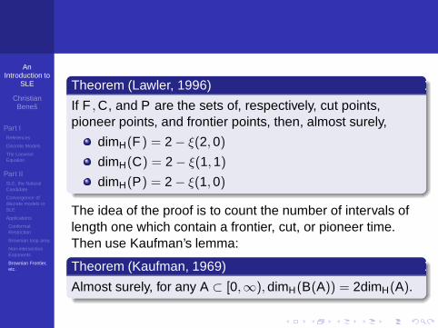
Theorem (Lawler, 1996)
If F ,C, and P are the sets of, respectively, cut points,pioneer points, and frontier points, then, almost surely,
dimH(F ) = 2 − ξ(2,0)
dimH(C) = 2 − ξ(1,1)
dimH(P) = 2 − ξ(1,0)
The idea of the proof is to count the number of intervals oflength one which contain a frontier, cut, or pioneer time.Then use Kaufman’s lemma:
Theorem (Kaufman, 1969)
Almost surely, for any A ⊂ [0,∞),dimH(B(A)) = 2dimH(A).
AnIntroduction to
SLE
ChristianBeneš
Part IReferences
Discrete Models
The LoewnerEquation
Part IISLE, the NaturalCandidate
Convergence ofdiscrete models toSLE
Applications
ConformalRestriction
Brownian loop area
Non-intersectionExponents
Brownian Frontier,etc.
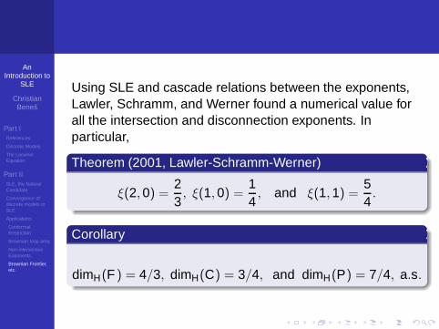
Using SLE and cascade relations between the exponents,Lawler, Schramm, and Werner found a numerical value forall the intersection and disconnection exponents. Inparticular,
Theorem (2001, Lawler-Schramm-Werner)
ξ(2,0) =23, ξ(1,0) =
14, and ξ(1,1) =
54.
Corollary
dimH(F ) = 4/3, dimH(C) = 3/4, and dimH(P) = 7/4, a.s.


![arXiv:1103.4728v1 [math.PR] 24 Mar 2011arXiv:1103.4728v1 [math.PR] 24 Mar 2011 Bessel process, Schramm-Loewner evolution, and Dyson model – Complex Analysis applied to Stochastic](https://img.pdfslide.us/doc/110x75/5f537d8bb93fe8613a385b60/arxiv11034728v1-mathpr-24-mar-2011-arxiv11034728v1-mathpr-24-mar-2011.jpg)