SAN FRANCISCO STATE UNIVERSITY

MATHEMATICS DEPARTMENT

http://math.sfsu.edu/

Working Paper No. 06-001

Bargaining in Continuous Time:

Holding Out for Concession and for Information

by

Jean-Pierre P. Langlois

January 13, 2006

Bargaining in Continuous Time:

Holding Out for Concession and for Information

by

Jean-Pierre P. Langlois*†

January 13, 2006

Abstract

This paper studies strategic bargaining in continuous time in order to allow

the of offers and acceptance to be true decision variables. The main technical timings

innovation is to decouple these timing decisions in order to study how each side can use

delaying tactics to wear the other down into concession. There are two main restrictive

assumptions: (1) players cannot use "explosive" strategies that could generate (with positive

probability) infinitely many moves in finite time; and (2) there is no arbitration for the

simultaneous acceptance of mismatched offers. It is simply ruled invalid. I construct and

characterize subgame perfect, perfect Bayesian, and sequential equilibria in the complete and

incomplete information cases respectively. Despite the stationarity of the game parameters,

and with or without an inside cost game option, I exhibit a multiplicity of equilibria that are

generically inefficient whether information is complete or not. I conclude that the uniqueness

and efficiency results of the standard Rubinstein model are jeopardized when the temporal

monopoly constraint is lifted.

JEL codes: C70, C78

Keywords: Bellman equation, continuous time, countervailing strategy,

finite state machine, survival function.

1

Bargaining in Continuous Time:

Holding Out for Concession and for Information

1 Introduction

In the strategic approach initiated by Rubinstein (1982) and Stahl (1972) bargaining

is pictured as a discounted repeated game and its solution involves an appropriate perfect

equilibrium concept. This has evident conceptual advantages over Nash's original axiomatic-

based solution: first, the outcome of bargaining is the result of strategic interaction between

selfish and rational actors rather than that of a process akin to arbitration. Second, bargaining

is often just a facet of a richer strategic interaction that may involve the power to hurt and

may not always be resolved as fairly as arbitration would aim for. And third, some temporal

aspects that are overlooked in the axiomatic approach are explicit in the strategic one.

However, the great benefits of the strategic approach to bargaining are mitigated by a

nagging simplification of the temporal picture: in most cases the players move sequentially at

fixed intervals of time, a modeling feature called "temporal monopoly". Since the value of

the solution depends explicitly on the length of the interval, this temporal picture is clearly

not neutral. But there is a deeper and more troublesome issue: could the very nature of the

solution depend on the assumption that moves are sequential and at fixed intervals of time,

therefore not subject to the players' decisions? Put another way, would theoretical predictions

be substantially different should the timings of offers and acceptance become explicit

decision variables? One reason this may be so is that the uniqueness and efficiency of the

Rubinstein solution can be traced directly to the cost of waiting an additional periodfixed

and to the resulting incentive for immediate acceptance. So, if the delays can be manipulated

strategically can uniqueness and efficiency evaporate altogether?

Interest in these issues is nothing new. Indeed, efforts at making the timing of offers

or acceptance true decision variables can be found in Cramton (1992), Perry and Reny

2

(1993), and Sakovics (1993). More recently, Wang (2000), Smith and Stacchetti (2003), and

Sandholm (2002) also frame these decisions within the time continuum. All these efforts

vary in underlying assumptions and methodology. From the assumption viewpoint, for

instance, Cramton allows the players to delay their offers but maintains the constraint of

alternating turns. And although it is not unreasonable to expect players to take turns in a

bargaining game, there is a subtle difference between allowing them and themconstraining

to do so. Smith and Stacchetti require that an offer be instantly accepted or rejected thus

precluding that it remains on the table for some time. But leaving an offer on the table while

attempting to wear down an opponent into acceptance may be an important strategic option

that should not be precluded, especially if the players have the power to hurt each other.

From a methodology viewpoint, for instance, one may pick a unit period and obtain

equilibria, then let the period length approach zero and examine the limit, as in Cramton. But

the limit of the solutions of the discrete case may not yield all solutions of the limit model, as

happens in the present paper. One may also frame the objective in the time continuum but

restrict attention to some classes of strategies, as in Smith and Stacchetti. This may be

enough for existence results but it leaves out a broader description of what behavior can be

involved in equilibrium. Finally, the solution concept itself can vary from Nash, to perfect, to

sequential, involving complete or incomplete information as in Wang (2000). It can also use

the weaker "epsilon-equilibrium" form that has been applied more generally to games of

timing, as in Laraki, Solan and Vieille (2005).

The results, primarily existence, uniqueness, and efficiency of equilibria, of course

vary with the assumptions and the methodology. But, more importantly, one must wonder

whether such results are only a reflection of the constraints on behavior. If one, for instance,

lets the period length approach zero in the original Rubinstein model, the limit solution

inherits the efficiency of the discrete one and is arguably a solution of a "continuous-time"

model. But, as I show in this paper, it is not be the only one and most others are inefficient.

Moreover, multiplicity or inefficiency can occur under temporal monopoly with various

3

additional assumption: Busch and Wen (1995), for instance, show how an inside cost game

can jeopardize both. And Coles and Muthoo (2003) reach similar conclusions with non-

stationary game parameters.

Ideally, one would want a model as free as possible of any timing constraint if the

issue is to understand whether uniqueness and efficiency are only the result of "artificial"

timing assumptions. But relaxing such constraints does not come without costs. Indeed, a

host of new issues arises from relaxing timing constraints: first, since offers can be accepted

at any time, as long as they are still on the table, the timing of offers and acceptance must be

independent decision variables. And, although offers should not be limited to the "take-it-or-

leave-it" kind, such offers should still be allowed. However, if an offer is to be accepted or

rejected "instantly" its recipient must make that move the offer. Butimmediately following

there is no single turn following an offer in the time-continuum. Second, in a framework

where an offer can remain on the table for some time, players must be allowed to withdraw it

instantly from the table if it is not taken. It thus becomes necessary to clarify the relative

timing of acceptance, rejection and withdrawal. Third, since alternating turns are no longer

the rule, simultaneous moves must be allowed. But how should they be resolved if they are

not compatible? For instance, what if the two sides simultaneously accept offers that do not

add up to the whole pie?

I argue that these issues affect the very definition of the player's very decision space

and I propose to extend it from simple offer, acceptance, and cost control moves to more

complex logical instructions such as "take it or leave it" or "if offered at least this much then

accept instantly." But if logical instructions can be the players' very decisions and if they can

be simultaneous, then they must be scrutinized for consistency and legality. Conceptually, it

is as if each side hands logical instructions to an agent who instantly meets the other side's

agent to decide whether any deal has actually been reached according to law and logic.

As the game unfolds, various events such as offers and cost adjustments take place

and become part of the history upon which the players plan their future moves. A strategy

4

therefore expresses how the logical instructions at any time result from the prior history of

the game. And it translates into a map from the time continuum, through the two sides'

logical instructions, into offer, cost, and acceptance state variables. Because an infinite

frequency of players' moves is ruled out by assumption, this map has isolated discontinuities.

This leads to a natural definition of the players' objectives as an expectation of acceptance by

one side or the other, appropriately discounted for delays, minus a possible expected cost of

waiting. In the time continuum this expectation is expressed as a Lebesgue-Stieltjes integral

up to the time-infinity.

Within this picture of time, action space, and objective function, I construct subgame

perfect equilibria (SPE) under perfect information, and perfect-bayesian (PBE) and

sequential equilibria under incomplete information. They involve "holding-out" behavior

akin to that predicted in war of attrition games: each side waits strategically, applying the

pressure of costs and delays, in the hope that the other side will make a better offer or will be

first to concede. The optimal waiting time strategy is probabilistic and given by an

exponential "survival" function with a parameter that depends on the game data and the

current offer and cost conditions. But a deterministic timing structure resembling the

Rubinstein framework is also possible if the players choose to adopt it. The difference is that

respecting the agreed upon timing scheme becomes part of the players' strategies instead of

being the fiat of the theorist. These findings suggest that Rubinstein's uniqueness and

efficiency results do not survive the relaxation of its temporal monopoly assumption.

Most of the results extend to the incomplete information case with finitely many

types on each side, although some results need to be qualified. For instance, a wide range of

offers is permissible in holding out SPEs whereas only extreme ones are possible in PBEs as

long as complete information has not yet been reached. Likewise, only a Nash equilibrium of

the cost game, if it is non-trivial, can be used in a PBE. This suggests that incomplete

information yields ungenerous and hurtful choices in equilibrium, and this also entails

inefficient delays. However, I show that complete information is reached in finite time.

5

2 Model and Assumptions

In the standard framework there are two players denoted and with symmetric roles3 4

but possibly different characteristics. Player makes offers to player , receives3 B − Ò!ß "Ó 43

share if accepts , receives share if he accept 's offer, and derives utility Ð" B Ñ 4 B B 4 ? ÐBÑ3 3 4 3

if is his share of the accepted offer. Since more is assumed better, utility is a strictlyB ?3

increasing function of its argument. The bargaining game may also involve an inside cost

game option with strategic variable (for ) and cost flow D − 3 - ÐD ß D Ñ Ÿ !3 3 3 3 4V bounded .

Acceptance by either side ends the game and the occurrence of any further costs.

2.1 Decisions as Logical Instructions

An offer by a player must stipulate its magnitude and the time when it is made. In the

discrete alternating turn framework there is no ambiguity as to when that offer can be

accepted or rejected since its recipient is next to move at a well specified time. But in

continuous time it is less clear. One approach adopted by Smith and Stacchetti (2003) is to

assume that an offer must be "instantly" accepted or rejected. This is appealing because it

requires no arbitrary built-in delays and bypasses any discussion of whether a rational player

might prefer to postpone acceptance. But in many bargaining situations an offer can remain

available, at least for some time, perhaps with a given deadline, when it is not immediately

accepted or explicitly rejected. So, requiring an immediate response for all offers is clearly

restrictive. Instead, I let the players decide for themselves whether an offer they make is to be

instantly dealt with or can remain available for some time. But this requires a formulation

that goes beyond simply stating an offer magnitude. It implies that statements such as "here

is my offer, take it or leave it " be explicitly part of the player's action space.now

Formally, an offer is a pair of magnitude made by player to hisÐB ß >Ñ B − Ò!ß "Ó 33 3

counterpart date . An offer of magnitude zero is legal and can serve several4 > − Ò!ß_Ñat

purposes such as withdrawing a prior offer. The notation means that no offer isÐg ß >Ñ3

tendered by at time and will be used to define the outcome of strategy. All by itself 3 > ÐB ß >Ñ3

6

doesn't say for how long will remain available and whether it comes with any contingencyB3

such as "take-it-or-leave-it." It is merely an element in a universe of discourse for theh

logical instructions that will form the players' decision spaces. So, 's counterpart should be3 4

able to accept 's offer whenever she likes as long as it is not withdrawn. Acceptance by is a3 4

non-empty signal denoted together with the time when it is issued, that is the pair .+ > Ð+ ß >Ñ4 4

Rejection, denoted , is also a non-empty signal signifying that makes the decision not toc+ 44

accept at that time, a move that must be distinguished from the lack of any acceptance

decision that will be denoted . Neither rejection nor lack of acceptance by affects 'sg 4 34

offer. But acceptance presumes that something is indeed available and will in fact require a

careful definition of player 's "current offer." Acceptance does not spell out exactly is3 what

accepted and is only, like offers, an element in the universe of discourse . Finally, a costh

decision by is a pair made up of a cost control and the time when it is3 ÐD ß >Ñ D − >3 3 3V

implemented, and it is an element of . As the game begins at time the two sides'h > œ !

offers and cost controls are assumed to be in a preexisting default state. For instance, each

side may be offering zero and be currently inflicting costs on the other. A null offer,

acceptance, or cost control has no effect on the current state of the correspondingÐg ß >Ñ3

variable which therefore remains in its prior state.

So, an offer followed at some time by an acceptance shouldÐB ß >Ñ = > Ð+ ß =Ñ3 4

unambiguously end the game with share for and for at time . But what aboutB 4 Ð" B Ñ 3 =3 3

immediate turnacceptance? In discrete time immediate acceptance would occur at =

immediately following . But in the time continuum there is no single time following time> =

> B = >. Immediate acceptance should thus mean that is considered accepted for any 3

arbitrarily close to decision . This seems only possible if the acceptance is issued at> +4

precisely the same time ( ) the accepted offer is tendered. But then, how does know= œ > 4

that an offer she hasn't yet seen will be satisfactory when she accepts it?

One can think of several avenues to deal with this issue, for instance: (1) establish

some delay between successive decisions. One drawback is that the value of is set by? ?= =

7

the theorist and is therefore arbitrary. Indeed, it is typically made to approach zero in a limit

argument that is an indirect way of adopting another option; (2) base acceptance on beliefs at

information sets representing simultaneous decisions. But it seems awkward to presume that

players in a bargaining game would accept an offer they haven't yet seen onunconditionally

the basis of their beliefs about what it will turn out to be. It should be preferable to wait even

a tiny instant in order to reach certainty; (3) weaken the solution concept to that of -%

equilibrium. Strategies can then involve waiting a tiny instant after an offer is made?=

before accepting it. The resulting cost can be made less than an arbitrary ; (4) allow players%

to issue decisions that are explicitly conditional on what their counterpart's simultaneous

decision turns out to be. In this last approach, each side instructs an to tender or acceptagent

offers on its behalf subject to contingencies. Whenever a decision is issued by either side, the

two sides' agents meet and execute jointly their instructions according to law and logic.1

Indeed, each side can issue "standing instructions" and only modify them from time to time

as they see fit. This is the approach investigated in this paper.

In this conceptual framework all offer, acceptance, and cost moves can be issued at

any time by players and and can be made conditional on each others' prior or3 4

simultaneous instructions. Player 's instructions at time therefore can use 's own3 > 4

simultaneous instructions as "input" to produce 's offer, acceptance, and cost moves as3

output. Formally, denotes the set of alll V3 3 3 3 3 3 3œ Ò!ß "Ó Ög × ‚ Ö+ ß c+ ß g × ‚ Ög ×a b a bpossible (offer, acceptance, and cost) moves by , any of which can be null. And if 3 H4

denotes the set of all possible instructions by , then 's instruction at time is a map4 3 >!3>

(1)! H l3>

4 3À Ä

that, given any possible simultaneous instruction , yields 's potential new offer ," H4>

4 3− 3 B

acceptance , and cost control decision at time , any of which may be the null . Player+ D > g3 3 3

3's own "action space" is then the set of all such maps .H !3 3>

8

A more practical description for is that it is a "finite state machine" (i.e., a!3>

computer program) that uses 's own instructions' to issue 's moves. It is therefore4 3

convenient to use pseudocode to describe these instructions. For instance

: offer (2)!3>

3"#œ B œ

means that 's decision is only to issue the unconditional offer at time regardless of 's3 Ð Ñ > 4"# 3

own instructions ( is not used in (2)). The symbol " : " represents an assignment of to" !4 3> >œ

the logical instructions on the right-hand side. If wishes to instantly accept this new offer,4

provided it is made, she could issue the instruction

: input ( 's instructions); if then (accept) (3)! " " !4 3 3 3> > > >

4œ 3 Ð œ Ñ +

with given by (2). If does issue the offer is made and 's agent issues the decision! !3 3> > "

# 33 Ð Ñ 4

+ 34, resulting in the instant acceptance of the offer. But perhaps only wishes to make a "take-

it-or-leave-it offer. In that case, he could issue instead

: input ; if then offer (4) ! " " !3 4 4 4> > > >

3"#œ Ð œ Ñ B œ

If the argument in (3) is the pseudocode in (4) and if the argument in (4) is the! !3 4> >

pseudocode in (3), then is tendered and accepted instantly with . But if deviates evenÐ Ñ + 4"# 3 4

slightly from (3) then makes no offer. In fact, even if 's old standing offer has magnitude ,3 3 "#

4 does not accepts it according to since it requires specifically . ! !4 3> >

So, formulae (3) and (4) are highly restrictive since the desired outcome only occurs

for a very specific pair of instructions. But these could easily be broadened. Instead of

requiring to issue just in (4) could draw a list of acceptable instructions by and3 4 3! f3>

3

replace the test by in (4). For instance, letÐ œ Ñ Ð − Ñ" ! " f3 3 3> > >

3

"input ; if then offer ", such that f ! " " !3 3 33 4 4 4> > > > "

#œ Ö œ Ð œ Ñ B B   ×

This set of instructions includes (4) and can modify (3) into 4

: input ; if then accept (5)! " " f4 3 3> > >

3 4œ Ð − Ñ +

Of course, can proceed similarly so that broader instructions on both sides can allow a3

successful offer and acceptance of the take-it-or-leave-it offer. In the most general case, !4>

9

can use as a "subroutine" and implement the resulting program rather than simply read 's"3> 3

script and decide whether it belongs to an acceptable set. Such an approach allows more

flexibility and more realism in the interaction between the two sides' respective agents but

requires good programming skills since must not "loop" and fail to yield an! !4 3> >a b

unambiguous outcome in , a development that is here assumed away.l3

In the most general game theoretic framework, moves can be probabilistic. And

finite-state machines can indeed involve probabilistic transitions between states. However, an

ambiguity could arise if acceptance by one side is made contingent on a probabilistic offer by

the other, since both sides' instructions must be executed simultaneously. To avoid this

situation it will be assumed that any such probability is resolved by an appropriate random

device to execution of the two sides' instructions. In essence, this means that severalprior

deterministic !4> 's could be issued at time , each with a probability.>

When instructions result in no offer, acceptance or cost control moves, all are deemed

null (denoted for ). It will be convenient to sometime write "offer " to indicate that g 3 g 33 3

issues no offer. But need not issue any instructions such as . In that case by3 œ g! !3 3> >

3

convention and this results in a null output. This is not the same as issuing "standing

instructions". In that case continuously issues the same knowing that it will result in a3 !3>

non-null output only when issues the desirable instructions. In all cases, the two sides'4

instructions at time (whether null or not) read>

! ! ! H H H> > >3 4 3 4œ ß − œ ‚ˆ ‰

and they result in an output denoted

_! l l l>3 4− œ ‚

made up of all three possible moves by each side, any of which may be null. The "legal"

operator that will be described in Assumption A2 below will be necessary to resolve some_

potential conflicts that could arise between the various moves. For instance, the two sides

could simultaneously make and accept "over-generous" offers that would add up to more

10

than the pie. These will be ruled illegal and will result in null offers and acceptance in . It_!>

will be convenient to write when the output is made up only of null moves. is_! _!> >œ g

called an "event" if at least one of its moves is non-null, formally if . is called an_! _!> >Á g

" -event" if one non-null move is in . The notation3 l3

offer (or accept , or set cost control to )! !3 4> >

3 3 3Ð Ñ È B + D

will indicate that yields the offer (or acceptance or cost control) by the! !3 4> >

3Ð Ñ B 3 before

legal operator is applied. " offer " instead means that the offer is indeed legal._ _!> 3È B

In this perspective, the instructions contained in are executed and resolved!>

instantly as if time is suspended while the two sides' respective agents interact. One could

instead assume that the interaction takes time but that the players cannot modify their

instructions while it lasts and this would not change the results. If, however, the time it takes

depends on the complexity of the instructions, then the results might be affected.

2.2 Strategies

denotes the history prior to time (note that gives2 œ Ö À = >× > 2> >! H= − strictly

time ). And will denote the set of all possible histories. A strategy for player is a> 3[ pure

map that, to any prior history , associates that player's contemporary< [ H3 3>À Ä 2

instruction . But it will be necessary to broaden the range of strategies in order to allow!3>

decisions that involve probabilities in both is decided and it is decided. So, if what when e3

is the set of random variables available to player , a strategy is a map3 randomized

< [ e H3 3 3À ‚ Ä

that, to any prior history , associates that player's contemporary decision with some2> >3!

proba Finitely many possible 's can be involved in such a lottery at time , andbility . !Ð Ñ3> !3

> >

!3> can be null if the lottery is about whether to issue any instruction at all.

Any random device used by is assumed privately monitored and independent of 's3 4

devices. However, the of the random devices used by either side can be publicparameters

knowledge. There is a subtle but important difference between randomization in the oftiming

11

an instruction and a randomization among several deterministic instruction at a given time: in

the first case, is monitoring a private device to decide whether to issue an instruction. In the3

second case, is issuing one of several non-null instructions . For example3 !3>

(accept)

<33Ð2 Ñ œ+ > œg>3

œ if otherwise

(6a))

means that accepts 's current off3 4 er at time . If is a random variable (with value true or) )

false) in , say with exponential distribution e3 ) -Ð   =Ñ œ / ! 3 =- of parameter , an -

event can only occur when the variable takes the value true. Consider instead, with fixed )

<3Ð2 Ñ œ> œ

g>3

3œ ! )) if

otherwise (6b)

with ! !3 3) ): (accept), with probability ; : (reject), with probability .œ + œ c+3 3

" "# #

In that case, an event does occur at whether the acceptance is issued or not. ) Of

course, other statements concerning 's offers and cost controls are generally involved in 3 <3.

As events are generated by strategies from a prior history, they become part of a

longer history. But in the time continuum, there is the potential for events becoming so2

frequent that there could be infinitely many within a finite history. Such a development is

called an "event explosion." In that case, at least one side must be generating the explosion.

So, a strategy (for ) is called "explosive" if there exists a strategy (for ) such that the< <3 43 4

pair can generate a history that contains infinitely manyÐ ß Ñ< <3 4 with positive probability 2>

3-events. The results of this paper require few significantly restrictive assumptions on the

strategies that players can adopt. The main restriction is

Assumption A1 (No Explosion): A player cannot use any explosive strategy.

In practice, this means that allowable strategies should include provisions that

preclude, or give probability zero, to the possibility of an event explosion. For instance, a

strategy that makes only one decision at only one time, like in (6), cannot generate any -<3 3

event explosion. But, more generally, mild statements can be included in the formulation of

12

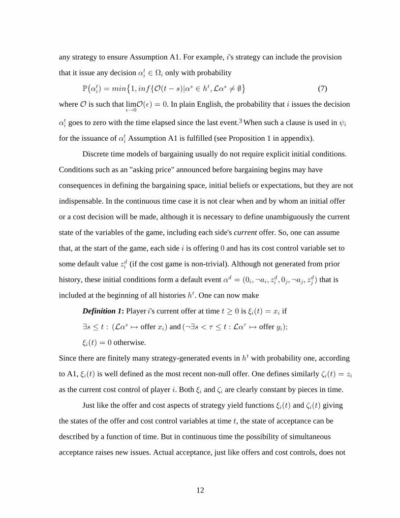
any strategy to ensure Assumption A1. For example, 's strategy can include the provision3

that it issue any decision only with probability! H3>

3−

(7) ! b !ˆ ˜ ™3> = >Ñ œ 738 "ß 380Ö Ð> =Ñl − 2 ß Á g_!=

where is such that . In plain English, the probability that issues the decisionb b %lim%Ä!

Ð Ñ œ ! 3

! <3>

3 goes to zero with the time elapsed since the last event. When such a clause is used in 3

for the issuance of Assumption A1 is fulfilled (see Proposition 1 in appendix).!3>

Discrete time models of bargaining usually do not require explicit initial conditions.

Conditions such as an "asking price" announced before bargaining begins may have

consequences in defining the bargaining space, initial beliefs or expectations, but they are not

indispensable. In the continuous time case it is not clear when and by whom an initial offer

or a cost decision will be made, although it is necessary to define unambiguously the current

state of the variables of the game, including each side's offer. So, one can assumecurrent

that, at the start of the game, each side is offering and has its cost control variable set to3 !

some default value (if the cost game is non-trivial). Although not generated from priorD3.

history, these initial conditions form a default event that is!. . .3 3 4 43 4œ Ð! ß c+ ß D ß ! ß c+ ß D Ñ

included at the beginning of all histories . 2> One can now make

PDefinition 1: layer 's current offer 3 at time is if>   ! Ð>Ñ œ B03 3

offer and offer b B cb= Ÿ > À C à= Ÿ > À È Èa b a b_! _!=3 37 7

otherwise.03Ð>Ñ œ !

Since there are finitely many strategy-generated events in with probability one, according2>

to A1, is well defined as the most recent non-null offer. One03Ð>Ñ defines similarly '3 3Ð>Ñ œ D

as the current cost control of player . Both and are clearly constant by pieces in time.3 0 '3 3

Just like the offer and cost aspects of strategy yield functions and giving0 '3 3Ð>Ñ Ð>Ñ

the states of the offer and cost control variables at time , the state of acceptance can be>

described by a function of time. But in continuous time the possibility of simultaneous

acceptance raises new issues. Actual acceptance, just like offers and cost controls, does not

13

just result from a one-sided strategy. Instead, actual moves result from the resolution of both

sides' instructions into a possible event . It is therefore necessary to describe precisely the_!>

legal operator mentioned before. It involves the cases when the players make over-_

generous offers and when the two sides simultaneously attempt to accept mismatched offers.

In either case, arbitration would be needed. But since arbitration schemes are let usarbitrary

make

Assumption A2 (No Arbitration):

_!> œ ˆ ‰! ! ! !3 4 4 3> > > >Ð Ñß Ð Ñ with the following three exceptions:

• Simultaneous over-generous offers are null:

if ( offer ) and ( offer ) and ( )! ! ! !3 4 4 3> > > >

3 4 3 4Ð Ñ È B Ð ÑÑ È B B B "

then (no offer ) and (no offer );_!> 3 4È g g

• A unilateral over-generous offer is null:4

if ( offer ) and ( no offer ) and ( )! ! ! ! 03 4 4 3> > > >

3 4 3 4Ð Ñ È B Ð Ñ È g B Ð>Ñ "

then no offer ;_!> 3È g

• Simultaneously acceptance of mismatched offers yields rejection by both:

if ( accept ) and ( accept ) and ( )! ! ! ! 0 03 4 4 3> > > >

3 4 3 4Ð Ñ È + Ð Ñ È + Ð>Ñ Ð>Ñ Á "

then (reject ) and (reject );_!> 3 4È c+ c+

These legal restrictions are implemented (as operator ) once both sides' instructions_

have been resolved into and respectively. It is therefore fruitless to include! ! ! !3 4 4 3> > > >Ð Ñ Ð Ñ

contingencies in either player's instructions about nullified decisions. Instead, each side

should carefully write its instructions to avoid seeing any of them nullified. The third

condition in A2 precludes any contentious simultaneous acceptance. Therefore, an event that

results in an acceptance ends the game. There can be no further events and the history is

final.

14

Now let " " mean that issues an acceptance (legal orT 7 ! !3 33 4ÐMÑ œ b − M À Ð ÑÑ È + 37 7

not) within the interval and let " " mean that legally acceptsM ÐMÑ œ b − M À È + 3T 7 _!3 3_ 7

within that interval . The probabilityM

J Ð>Ñ œ Ò!ß >Ñ3 3 Tˆ ‰_

is a distribution function which, together with the similar , describes the probabilistic stateJ4

of acceptance of the game. 5 However, discrete probabilities of acceptance at specific event

times are also allowed and result in right-hand side discontinuities of at such times. ForJ3

example, suppose that plans to never issue any acceptance, so that , and that issues4 J ´ ! 34

an acceptance at a specific time . Then+3 )

ifif

J Ð>Ñ œ! > Ÿ" > 3 œ )

)

But, instead of being a specific time can be a random variable, for instance with)

exponential distribution of parameter . In that case .- J Ð>Ñ œ " /3 >-

A discontinuity is interpreted as a discrete probability?J Ð Ñ œ J Ð Ñ J Ð Ñ !3 3 3) ) )

of acceptance by at time . And, although variations of represent random elements in3 J) 3

acceptance, they have different interpretations: a continuous variation is about the timing of

an acceptance while the second is about the decision to accept at the time of the

discontinuity. Indeed, a discrete probability of acceptance at a specific is an -event?J Ð Ñ 33 ) )

observable by , while a continuous is only about whether and when an -event may4 J Ð>Ñ 363

take place.

2.3 Player Objective

Any history , through the induced strategy profile , determines2 œ Ð ß Ñ> > > >3 4G < <

further offer, cost, and acceptance behavior that translate at future time into currentÐ> Ñ7

offer, cost and acceptance probability. The superscript " " will be used to indicate>

developments according to this induced , so that G> 0 7 0 7 G3> >

3Ð Ñ œ Ð> l Ñ >. A "path" at time

is a map

15

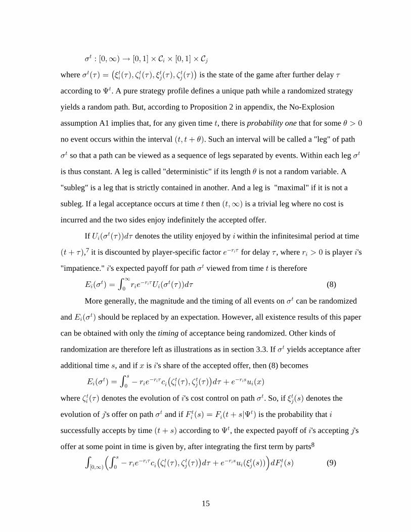
5 V V>3 4À Ò!ß_Ñ Ä Ò!ß "Ó ‚ ‚ Ò!ß "Ó ‚

where 5 7 0 7 ' 7 0 7 ' 7 7> > > > >3 3 4 4Ð Ñ œ Ð Ñß Ð Ñß Ð Ñß Ð Ñˆ ‰ is the state of the game after further delay

according to G>. A pure strategy profile defines a unique path while a randomized strategy

yields a random path. But, according to Proposition 2 in appendix, the No-Explosion

assumption A1 implies that, for any given time , > there is that for some probability one ) !

no event occurs within the interval . Such an interval will be called a "leg" of pathÐ>ß > Ñ)

5> so that a path can be viewed as a sequence of legs separated by events. Within each leg 5>

is thus constant. A leg is called "deterministic" if its length is not a random variable. A)

"subleg" is a leg that is strictly contained in another. And a leg is "maximal" if it is not a

subleg. If a legal acceptance occurs at time then is a trivial leg where no cost is> Ð>ß_Ñ

incurred and the two sides enjoy indefinitely the accepted offer.

If denotes the utility enjoyed by within the infinitesimal period at timeY . 33a b5 7 7>Ð Ñ

Ð> Ñ7 , it is discounted by player-specific factor for delay , where is player 's7 / < ! 3<3

37 7

"impatience." 's expected payoff for path viewed from time is therefore 3 >5>

(8)I Ð Ñ œ < / Y .3 3 3> <

!

_5 7 7' 37 a b5>Ð Ñ

More generally, the magnitude and the of all events on can be randomized timing 5>

and should be replaced by an expectation. However, all existence results of this paperI Ð Ñ3>5

can be obtained with only the of acceptance being randomized. Other kinds oftiming

randomization are therefore left as illustrations as in section 3.3. If yields acceptance after5>

additional time , and if is 's share of the accepted offer, then (8) becomes= B 3

I Ð Ñ œ < / - Ð Ñß Ð Ñ . / ? ÐBÑ3 3 3> < > > < =

!

=

3 3 45 ' 7 ' 7 7' 3 37 ˆ ‰where denotes the evolution of 's cost control on path denotes the' 7 03 4

> >Ð Ñ 3 Ð=Ñ5>. So, if

evolution of 's offer on path is the probability that 4 J Ð=Ñ œ J Ð> =l Ñ 35> and if 3> >

3 G

successfully accepts by time according to , the expected payoff of 's accepting 'sÐ> =Ñ 3 4G>

offer at some point in time is given by, after integrating the first term by parts8

(9)' 'Ò!ß_Ñ !

=

3 3< > > < = > >

3 3 4 4 3Š ‹ˆ ‰ < / - Ð Ñß Ð Ñ . / ? Ð Ð=ÑÑ .J Ð=Ñ3 37 ' 7 ' 7 7 0

16

œ / J Ð=Ñ J Ð_Ñ < - Ð=Ñß Ð=Ñ .= ? Ð Ð=ÑÑ.J Ð=Ñ'Ò!ß_Ñ

< = > > > > > >3 3 3 4 4 33 33

3 Š ‹a b ˆ ‰' ' 0

Formula (9) is well defined for any path as a Lebesgues-Stieltjes integral, since

/ ? Ð Ð=ÑÑ< = >3 4

3 0 is clearly measurable. But it requires a careful interpretation at common

discontinuities of and (see Section 3.1 and Proposition 3 in appendix). A symmetric04 3> >J

formula involving the evolution of 's offer and the distribution function gives the3 Ð=Ñ J Ð=Ñ03 4> >

expected payoff that accepts. And the expected payoff that neither side ever accepts is4

Ð_Ñ / < - Ð=Ñß Ð=Ñ .=F ' '> < = > >Ò!ß_Ñ 3 3 3 4' 3 ˆ ‰

where is the "joint survival" function that expresses how longF> > >3 4Ð=Ñ œ " J Ð=Ñ J Ð=Ñ

the game lasts before one side or the other accepts. Adding up all three cases yields

(10)I Ð Ñ / .K Ð=Ñ3> < = >

Ò!ß_Ñ 345 œ ' 3

with .K Ð=Ñ œ ? Ð=Ñ .J Ð=Ñ ? " Ð=Ñ .J Ð=Ñ - Ð=Ñß Ð=Ñ Ð=Ñ.=34 4 3 3 4 3 4> > > > > > > >

3 3 3ˆ ‰ ˆ ‰ ˆ ‰0 0 ' ' F

The infinitesimal is simply the expected value that either side accepts minus.K Ð=Ñ34>

the expected cost, all discounted appropriately in the integral. In the incomplete information

case there will be two sets of types and and the players will entertain beliefs \ ] , Ð>Ñ   !4

such that (and similarly for ). Objective (10) will then generalize to!4−]

, Ð>Ñ œ "4 \

(11)I Ð Ñ œ / .K Ð=Ñ3> < = >

4−Ò!ß_Ñ 345 !

]

, Ð>Ñ4' 3

for type . Of course, the beliefs will 3 − \ be appropriately updated by Bayes' law when

discussing perfect Bayesian equilibria.9

2.4 A First Example

Let the players' strategies be such that (constant) and 0 '3 3> ‡ > ‡

3 3Ð=Ñ ´ B Ð=Ñ ´ D

(constant), and symmetrically for (with ). Further assume that issues an4 B B " 33 4‡ ‡

acceptance at random time with exponential density of parameter , and) .3 !

symmetrically for . After history , since the probability of acceptance by within the4 2 3>

infinitesimal at time is and the (independent) probability that has not yet.= = / .= 4.3 =.3

accepted is , . Moreover . In this case/ .J Ð=Ñ œ / .= Ð=Ñ œ / = > Ð Ñ= > Ð Ñ=3 3

. . . . .4 3 4 3 4. F

17

I Ð Ñ œ / ? ÐB Ñ ? Ð" B Ñ - ÐD ß D Ñ .=3 3 3 4 3 3> Ð< Ñ= ‡ ‡ ‡ ‡

!

_

4 3 3 45 . .' 3 3 4. . ˆ ‰ œ

. .

. .3 3 4 3 34 3 3 4

‡ ‡ ‡ ‡

3 3 4

? ÐB Ñ ? Ð"B Ñ- ÐD ßD Ñ

<

Now, let us define the important quantity

(12)A3 3 4 3 4- ÐD ßD Ñ< ? ÐB Ñ? Ð"B Ñ? ÐB ÑÐB ß B ß D ß D Ñ œ 3 3 4 3 3 4

3 3 3 4

and let us assume that chooses , then . In that case, 4 œ ÐB ß B ß D ß D Ñ I Ð Ñ ´ ? ÐB Ñ 3. A 54 3 3 33 4 3 4 4‡ ‡ ‡ ‡ > ‡

is made indifferent between waiting with the given exponential distribution or accepting at

any time. A symmetric argument also holds for given the symmetric . This example will4 .3

be generalized in the next section to obtain a subgame perfect equilibrium.

3. Bargaining with Perfect Information

Much of strategic bargaining theory was initially developed with perfect information.

It is therefore reasonable to first extend this case to continuous time. It is also easier to

discuss the characterization of optimal acceptance behavior without the added complexity

arising from continuous Bayesian updating. The methodology developed in this section

exploits the definition of path in dynamic programing fashion: in order to optimize their

objective, the players can concentrate on optimizing their behavior within each leg knowing

that the optimization problem they will face at the start of the next leg will be structurally

identical. The resulting optimality condition is often called a Bellman equation. In the next

section, this dynamic programming approach is made precise through Lemma 1.

3.1 Bellman Equation and Survival Functions

Because there can be no left-discontinuity in or one can always writeJ J3 4> > 10

(13)I Ð Ñ / .K Ð=Ñ / .K Ð=Ñ3> < = > < = >

Ò!ß Ñ Ò ß_Ñ34 345 œ ' ') )

3 3

And since , and describe conditional probabilities one can also writeJ3> >F

(14a).J Ð =Ñ œ Ð Ñ.J Ð=Ñ3> >

3>) F ) )

and (14b)F ) F ) F> > >Ð =Ñ œ Ð Ñ Ð=Ñ)

and thus . It follows from changing variables in (13) that.K Ð =Ñ œ Ð Ñ.K Ð=Ñ34> >

34>) F ) )

18

(15) I Ð Ñ œ / .K Ð=Ñ / Ð ÑI Ð Ñ3 3> < = > < > >

Ò!ß Ñ 345 F ) 5')

) )3 3

Formula (15) has important consequences. he so-called Bellman In particular, t

Equation obtains when writing that the maximum for the left-hand side of (15) is reached

when maximizing the sum on the right-hand side. 11 A subgame perfect equilibrium (SPE) is

a strategy profile that forms a Nash equilibrium in all subgames. But a subgame is the

bargaining game itself beginning at time with some prior history . So, a SPE must be> 2>

such that I Ð Ñ 3 43>5 , or its expected value, is maximized by 's induced strategy in response to 's

induced strategy In order to obtain such SPEs one can proceed in dynamic programmingÞ

fashion: assuming that the optimization problem is "solved" for the future it is enough to5>)

identify an optimal and the optimal behavior within .) )Ò!ß Ñ 12

In order to operationalize this approach, it is necessary to analyze precisely the nature

of the integral over in (15). Ò!ß Ñ) First, if denotes the discrete probability that issues an: 33>

acceptance at precisely time , and then is the probability of null> : :0 03 4> >Ð!Ñ Ð!Ñ ", 3 4

> >

acceptance is therefore the probability of . The discontinuity ?J !3 3 4> > >Ð Ñ œ : Ð" : Ñ non-null

acceptance of th 04>Ð!Ñ J ! = = œ !. With the symmetric translate at into a "mass"? 4

>Ð Ñ 3=

?K Ð!Ñ œ ? Ð!Ñ ? " Ð!Ñ34 4 3> > >

3 3: Ð" : Ñ : Ð" : Ñ3 4 4 3> > > >ˆ ‰ ˆ ‰0 0 (16a)

and, by Proposition 3 in appendix

(16b)' 'Ò!ß Ñ Ð!ß Ñ

< = > > < = >34 34 34) )

/ .K Ð=Ñ œ K Ð!Ñ / .K Ð=Ñ3 3?

Second, let

9 3> >Ð=Ñ œ " ˆT3Ð>ß > =щ

be the probability that issues no acceptance within the leg according to .3 Ð>ß > =Ñ G> can93>

be called 's "survival" function must clearly be continuous3 within the leg. It for all = − Ð!ß Ñ)

since only the of acceptance is random and a discontinuity would indicate an event.timing 13

Moreover, offers and costs controls are constant for 0 and can be denoted= − Ð ß Ñ)

0 '3 3 3 3 3 4> > > > > >

3Ð=Ñ ´ B Ð=Ñ ´ D - D ß D, , . With these notation one has and - ´3> ˆ ‰ 14

Lemma 1: Assume that is a leg. ThenÐ>ß > Ñ)

19

' 'Ð!ß Ñ Ð!ß Ñ

< = > > < > > > > >34 4 3 343) )

)/ .K Ð=Ñ œ Ð! Ñ / Ð Ñ ? ÐB Ñ Ð! Ñ Ð=Ñ. Ð=Ñ3 3ˆ ‰F F ) F 9 ,

with (17). Ð=Ñ œ / ? Ð" B Ñ ? ÐB Ñ . - < ? ÐB Ñ Ð=Ñ.=, 934 3 4 3 4 4> < = > > > > >

3 3 3 33 Š ‹ˆ ‰ ˆ ‰94

>Ð=Ñ

Discontinuities translate into on theProof: F>Ð! Ñ œ " Ð Ñ Ð Ñ > >3 4? ?J ! J !

previously defined . Thus for all F ) F> > > 3, , and = − Ð!ß Ñ .J Ð=Ñ œ Ð! Ñ9 94 3

> >Ð=Ñ. Ð=Ñ

.K Ð=Ñ œ Ð=Ñ. Ð=Ñ34 4 3> > >F> >

3 4Ð! Ñ ? BŠ ˆ ‰9 9

? " B 3 3>ˆ ‰9 9 9 93 4 3 3 4

> > > > >Ð=Ñ. Ð=Ñ - Ð=Ñ Ð=Ñ.=‹Integrating by parts the term in (since is continuous) yields the result. . Ð=Ñ Ð=Ñ9 93 4

> >/< =3 �

Formulae (15) and (16b), together with Lemma 1, will be used to construct perfect

equilibria.

3.2 A Subgame Perfect Equilibrium

The discrete-time Rubinstein theory may have promoted the belief that there is an

essentially unique rational solution to the strategic bargaining problem and that it is efficient,

at least in the stationary and perfect information case. However, none of this remains true in

continuous time. As the results below will show, the very possibility of randomization in the

timing of acceptance yields a vast class of SPEs that are generically inefficient.

The "countervailing" strategy defined below generalizes the example of §2.4.

Definition 1: A strategy (for player ) based on offer countervailing <4 4‡4 B − Ò!ß "Ó

and cost control is defined by : such that:D − Ð2 Ñ œ4 >‡ >

4 4 4V < !

• "Initially offer and set cost control to for all times." Formally:B D4 4‡ ‡

offer set cost control ; (18a)!4! ‡ ‡

4 4: œ ˆ ‰ˆ ‰ ˆ ‰B • D

• "Accept instantly . ˆ ‰" B4‡ 15 Formally:

(accept) ; (18b)ˆ ‰ ˆ ‰ ˆ ‰0 ! !3 3 44 4‡ > ‡ >

3 4Ð>Ñ " B ” B œ " B Ê +œ È œoffer :

• Otherwise, "on each leg , wait with exponential distribution of parameterÐ>ß > Ñ)

". . A4 3 3 4> >œ ß D ß Dˆ ‰B ß B3 4

> > 16 Formally:

:ˆ ‰B Ð= œ Ñ Ê Ð œ +3> " B • Ñ (accept) (18c)4

‡ >4 47 !

where is a random variable with distribution .7 ) 7− Ð!ß Ñ Ð   =Ñ œ / =.4

20

This last condition can also be expressed on the resulting function that must satisfy94>

. .= œ ! . Ð=Ñ ´ !9 .4>

4 9 ,4 34> > or (18d)

By extension, the survival function countervailing. The first main result is94> will be called

Theorem 1: Countervailing strategies form a subgame perfect equilibrium.

since the initialProof: Without loss of generality, one can assume that B B "3 4‡ ‡

offers would otherwise be null and the default would be used instead of andB œ B œ ! B3 4. . ‡

3

B4‡ throughout this argument.

countervailingAssume now that uses her strategy. If at any time 's current offer4 > 3

reaches .ˆ ‰" B 4 B then instantly (and successfully) accepts. In that case 4 4‡ ‡17 I Ð Ñ œ ? Ð Ñ3 3

>5

Otherwise, for any path beginning at time , there is probability one that for some 5 )> > !

Ð>ß > Ñ . Ð=Ñ ´ !) , is a leg. Within that leg, it was observed that .94> =Ð=Ñ œ / .4 results in 34

>

Moreover, since results in a continuous acceptance distribution function , any<4 4J

discontinuity at can only involve 's acceptance of .! 3 K Ð!Ñ œ J ! ? Ð ÑB Ð Ñ B4 4‡ > ‡

3 and yields? ?34>

3

And since , by Lemma 1 and by (15)?J ! " Ð! Ñ3>Ð Ñ œ F>

I Ð Ñ œ J ! Ð! Ñ / Ð Ñ ? Ð Ñ / Ð ÑI Ð Ñ3 3 3> > < > < > >5 F F ) F ) 5Š ‹? 3

> ‡4Ð Ñ B3 3) ) )

(19) œ " / Ð Ñ ? / Ð ÑI Рш ‰ ˆ ‰< > < > >3 3

3 3) ) )F ) F ) 5B4‡

Let be the successive event times generated on path by 's strategy. If there isÐ Ñ 3) 58 8−>

none or finitely many, use an arbitrary sequence of approaching . Iterating (19) yields)8 _

(20)I Ð Ñ œ " / Ð Ñ ? / Ð ÑI Ð Ñ3 8 3 8 3> < > < > >5 F ) F ) 5ˆ ‰ ˆ ‰3 8 3 8 8) ) )B4

‡

By Proposition 4 in appendix, . And, since is clearly bounded,lim8Ä_

< >8 3/ Ð Ñ œ ! I3 8) F )

I Ð Ñ œ ? 33 3 3>5 <ˆ ‰B4‡ . Since this holds for any strategy for player , the countervailing strategy

is a best reply after any history . 2> �

Extremal Equilibria): Corollary 1 Ð If then the SPE of Theorem 1 isB œ !4‡

extremal for .3

Player 's expected utility always reduces to which is theProof: 3 ? Ð!ÑI Ð Ñ œ3>5 3

minimum can guarantee himself by accepting 's last offer at any time. 3 4 �

21

Note that In typicalB œ B œ !3 4‡ ‡ provides an extremal equilibrium for sides.both

applications extremal equilibria are used as trigger threats: both sides play according to some

agreed upon "scenario" and defection is punished by reversion to an extremal equilibrium of

the deviating side. The next result shows how such a construction can be achieved here.

Corollary 2 ( ):Efficient Equilibria For any and cost controls and theB − Ò!ß "Ó D D3 3 4‡ ‡

following strategy profile forms a SPE.

at issue> œ !

: input ; if set ! " "3 4 4! ! ! ‡

3œ Ð œ D!4!

3 3Ñ B !then offer else offer and .

: then accept else .! !4 3! !

4œ Ñ +input ; if offer and set " "3 3! ! ‡

4 4Ð œ ! D

use countervailing strategies based on , , , and .a> ! Ð>Ñ Ð>Ñ Ð>Ñ Ð>Ñ0 0 ' '3 4 3 4

in the offer Proof: If and do issue and these result immediately accepted.3 4 B!3!

3!4!

This yields immediate utilities and . Any other decision by? Ð" B Ñ   ? Ð!Ñ ? ÐB Ñ   ? Ð!Ñ3 3 3 4 3 4

3 ! 4 results in nonacceptance and the offer followed by countervailing behavior on 's part4

with expected utility for from then on, clearly not an improvement at . The? Ð!Ñ 3 > œ !3

argument is similar for . And reversion to countervailing behavior provides an SPE. 4 �

A consequence of Corollary 2 is that, in the continuous time framework and under the

assumptions of this paper, strategic bargaining allows efficient outcomes but does not yield

uniqueness since any sharing of the pie can be sustained by a SPE.

Theorem 2 has conceptual consequences as well: first, it may seem awkward that the

parameter of 's survival function be given by a quantity that only involves 's game. A4 34 3

parameters. Indeed, the denominator of is only a measure of how far appart the two sidesA3

are, but its numerator is the total cost flow of - his actual cost of bargaining plus his3 -3

opportunity cost of not accepting 's offer. One might instead expect that should hold out as4 4

a function of own costs. But that would be a misconception. The reason 's survivalher 4

function is given by 's cost parameters is that her strategy is to pressure with expected3 3

accumulating costs, by delaying her own acceptance, to wear him down into giving up.

22

Second, Theorem 1 holds for any pair of offers such that B B "3 4‡ ‡ , whereas

immediate acceptance means that . The first condition is arguably more genericB B œ "3 4‡ ‡

than the second. If the two sides come to the bargaining table without prior exchange, and

with some idea of what offer they wish to make, it is more likely that the two won't exactly

add up to the whole pie. And all such pairs can be supported by a countervailing SPE. It is

tempting to object that, knowing this, the two sides would be both better off choosing offers

that result in an efficient outcome. But the process of choosing such offers is precisely what

is modeled in this paper and fails to identify a single efficient bargain.

3.2 Optimal Acceptance Behavior

A SPE based on a threat of reversion, as in Corollary 2, need not involve immediate

acceptance. Instead, some "scenario" can be implemented, until some deterministic or

probabilistic end, and be sustained by an appropriate threat. Such a scenario may involve

various offers and cost control adjustments, as well as a continuous or discrete-time

probabilistic acceptance strategy. However, although the parameters of probabilistic behavior

may be public knowledge, the random variables governing it are here assumed privately

monitored. So, if 's expected acceptance behavior is given by some 3 93> within some leg

Ð>ß > Ñ 4) , all that can observe is the occurrence of an acceptance or a rejection. A trigger

threat, therefore, cannot rely on 's conformance to any specific that can never observe3 493>

directly. This means that will undoubtedly choose in order to optimize his expected3 93>

payoff within , . It is thus useful to understand what optimal "shapes"Ð>ß > Ñ) ceteris paribus

93> can take. This section discusses this issue when the following holds:

for both on the leg Condition AP (Agreement is Preferred): 3 Ð>ß > Ñ)

- < ? ÐB Ñ !3 4> >

3 3

Condition AP holds if there is a positive cost flow ( ) to not reaching- !3>

agreement, regardless of whether that cost can be manipulated strategically, or if there is an

opportunity cost because the offered bargain is better than not having one ( ).? ÐB Ñ !3 4>

23

Lemma 2 and the resulting Theorem 2 give a useful characterization of equilibrium behavior

under condition AP: within each closed subleg of a deterministic leg, either both players

countervail each other or they are "non-acceptant," meaning that their probability of

acceptance is nil.

, , is a closed subleg,Lemma 2: Assume that condition AP holds, that Ò>ß > Ó !) )

and that and the integral (here for ) reaches a minimum. for each of3 4 3 Ð=Ñ. Ð=Ñ'! 3 34

> >)9 ,

Then, and must be constant or countervailing.9 93 4> >Ð=Ñ Ð=Ñ simultaneously

LetProof: , and for all let:. A )4 3 3 4> >œ B ß D ß D ! = − Ò!ß Óˆ ‰

3 4> >ß B

, .34 4> < = >

3 4Ð=Ñ œ / Ð=Ñ Ð< ш ‰Š ‹? Ð" B Ñ ? ÐB Ñ3 33 4> > 3 9 9'

!

=< >

4/ Ð Ñ.=37 7 (21)

Clearly on and one easily verifies that is as in (17). Moreover, ) ,34 34> >Ð=Ñ ! Ò!ß Ó . Ð=Ñ

(22)' '! !3 34 3 34 34 34

> > > > > >) )9 , 9 ) , ) , , 9Ð=Ñ. Ð=Ñ Ð Ñ Ð=Ñ.œ Ð Ñ Ð!Ñ Ð=Ñ3

>

after integrating by parts (since . There are two cases:9 ,3 34> > and are continuous)

(i) If is decreasing on according to Proposition 5 in appendix,9 )3> strictly Ò!ß Ó then,

, 9 )34 3> > must be constant for the last integral in (22) to reach an extremum given . ThisÐ Ñ

implies that is. Ð=Ñ œ !, 9 934> and countervailing. Since is strictly decreasing,4 4

> = >Ð=Ñ œ / .4

,43> must be constant for an extremum to be reached in (22) written for , 4 mutatis mutandis

and is countervailing.93> =Ð=Ñ œ / .3

(ii) If is decreasing on then there must be some subleg, call it9 )4> not strictly Ò!ß Ó

Ò!ß Ó . Ð=Ñ œ / - < ? ÐB Ñ .=) 9 , again, with 1. But and the integral4> ´ 34 3 4

> < = > >3 3

3 ˆ ‰ (23)' '

! !3 34 3 4 3> > > > < = >

3 3

) )9 , 9Ð=Ñ. Ð=Ñ œ - < ? ÐB Ñ / Ð=Ñ.=ˆ ‰ 3

can only reach an extremum when is constant by Proposition 5 (with ).93> < =.0Ð=Ñ œ / .=3

But 1 since . The same holds when exchanging and 9 93 3> >´ Ð!Ñ œ " 3 4. �

The integral that is minimized in Lemma 2 is only one term in the Bellman equation

(15). But knowing the optimal shapes of on reduces the optimization problem to a93> Ð!ß Ñ)

choice of boundary value at . Theorem 2 shows that, within a maximal leg, countervailing)

24

and non-acceptant behaviors can only cohabit in a very precise way and that they correspond

to different types of payoff expectations. One has

is a maximal deterministic legTheorem 2: Assume condition AP and that Ð>ß > Ñ)

of a SPE-generated path Then, there exists such that 5 / )>. and , ! Ÿ Ÿ for both mutatis3 4

mutandis:

(i) for and both sides are countervailing;I Ð Ñ ´ ? ÐB Ñ = − Ð!ß Ñ3>= >

3 45 /

and (ii) for and both sides are non-acceptant.I Ð Ñ ? ÐB Ñ = − Ð ß Ñ3>= >

3 45 / ) 18

Proof: In any SPE one must have for all since canI Ð Ñ   ? ÐB Ñ3>= >

3 45 = − Ð!ß Ñ 3)

always accept B4> at any time. And since there can be no mass within Ð!ß Ñ) by definition of a

leg one always has, or any :by (15) and by Lemma 1, f ! = = / )

I Ð Ñ œ ? ÐB Ñ / Ð Ñ Ð Ñ I Ð Ñ ? ÐB Ñ3 3 3 3>= > < >= >

4 43 4>= >=5 9 9 53/ // / ˆ ‰

(24) Ð Ñ. Ð Ñ'! 3 34

>= >=/9 7 , 7

Since does not , its very shape does not influence the parameters of the4 observe 93>=

optimization of . Therefore, the maximization by of always involvesI Ð Ñ 3 I Ð Ñ3 3>= >=5 5/ 19

the minimization over in of the integral in (24) given any . By Lemma 2,9 93 3>= >=Ò!ß Ó/ Ð Ñ/

this yields two cases:

(i) If is countervailing then the integral in (24) is nil. And if94>=

I Ð Ñ ? ÐB Ñ Ð Ñ œ " ´ "3 3>= >

4 3 3>= >=5 9 9/ then (24) is maximum for . But is not/

countervailing and neither can be by Lemma 2. So, and9 54>=

3>= >

3 4I Ð Ñ œ ? ÐB Ñ/

I Ð Ñ ´ ? ÐB Ñ = − Ò!ß Ó3>= >

3 45 / for .

Conversely, if then . And since isI Ð Ñ ´ ? ÐB Ñ Ð Ñ. Ð Ñ œ !3>= >

3 4 ! 3 34 3>= >= >=5 9 7 , 7 9' /

continuous positive on , (a.e.) and the continuous must satisfy theÒ!ß Ó . Ð Ñ ´ !/ , 7 934 4>= >=

countervailing condition (18d). By Lemma 2, must also be countervailing.93>=

(ii) If in then (23) and (24) yield9 /4>= ´ " Ò!ß Ó

I Ð Ñ œ ? ÐB Ñ / Ð Ñ I Ð Ñ ? ÐB Ñ3 3 3 3>= > < >= >

4 43>=5 9 53/ // ˆ ‰

(25) - < ? ÐB Ñ / Ð Ñ.ˆ ‰3 4> > < =

3 3 ! 3>=' /

3 9 7 7

25

Again, for any the integral in (25) must be minimized but this can only occur93>=Ð Ñ/

with a constant which must be identically by continuity. Since by93>=

3 4> >

3 3" - < ? ÐB Ñ !

the assumed AP, one must have . And by continuity in , this last strictI Ð Ñ ? ÐB Ñ3 3>= >

45 //

inequality must hold within some neighborhood of . Conversely, this inequality precludes a/

countervailing by (i) and implies in that neighborhood.9 93 3>= >= ´ "

Finally, assume the strict inequality for for simplicity.I Ð Ñ ? ÐB Ñ − Ð!ß Ó3 3>= >

45 7 /7

Replacing in (25) yields:93>= ´ "

(26)! - < ? ÐB Ñ Ÿ - < I Ð Ñ œ / - < I Ð Ñ3 4 3 3> > > >= < > >=

3 3 3 3 3 35 537 7a bIt follows that must be with . It can therefore never decrease back toI Ð Ñ3

>=5 77 increasing

? ÐB Ñ3 4> . So, countervailing behavior cannot follow non-acceptant behavior within a same leg,

but it can precede it as stated. �

In the continuous time bargaining framework, perfect equilibria can only involve

two possible kinds of acceptance behavior on a deterministic leg according to Theorem 2:

both sides are either countervailing or non-acceptant. These are two forms of "holding-

out" behavior: in the first case, both sides hold-out in the hope that the other will be first

to concede; in the second, they hold-out in the expectation of a better future. And under

condition AP, if the players are not countervailing on a leg their expected payoffs must

be with time. This is not surprising since non-acceptant behavior yields eitherincreasing

accumulating cost or the opportunity cost of not accepting sooner. And- ! ? ÐB Ñ !3 4> >

3

these are not compensated by some probability that the other side will accept along the

way according to countervailing. So, each side must be incurring these costs in the

expectation of a better future at the end of the leg, perhaps as a better offer or as a

discrete probability of the other side's accepting. As this better future draws nearer, one's

expected payoff increases. If instead the players are countervailing then their expected

payoffs are held to the constant utility of the other side's current offer.

3.3 A Second Example

26

Consider the following Rubinstein-like negotiating framework: the two sides "agree"

that they will alternately make offers at regular intervals of time of given length ,) !

perhaps with going first. They also agree that when makes an offer to , instantly3 3 4 4

withdraws his own last offer to (i.e. adopts offer magnitude ). Although 's offer remains3 ! 3

on the table until 's next turn to make one, neither side is expected to accept or even speak4

between turns. Indeed, if anyone deviates from this "scenario", for instance by not speaking

at their turn or not making the expected offer, they both instantly revert to countervailing

behavior on the basis of their last offers and cost controls, a well known SPE.

There are many possibilities regarding the choice of and the two sides' successive)

offers. For simplicity, let us assume here that the two sides stick stubbornly to offers B !3‡

and such that and to controls and resulting in costs thatB ! B B " D D -   !4 3 4 3 4 3‡ ‡ ‡ ‡ ‡ ‡

they impose on each other from the very start. Finally, assume that each side accepts the

other side's offer at each of his turns with probability (for ). So, if is a time at which : 4 > 34

receives 's offer and may accept it rationally with probability , one needs by (15)4 B : !4‡

3

(27)I Ð Ñ œ ? ÐB Ñ3 3> ‡

45

œ 5 / : ? Ð" B Ñ Ð" : Ñ 5 / ? ÐB Ñ3 4 3 4 3 3< ‡ < ‡

3 43 3) )Š ‹ˆ ‰

with since . This requires that5 œ Ð" / Ñ I Ð Ñ œ ? ÐB Ñ3 3 3< ># ‡-

< 43 3

‡

3

) )5

(28): œ4Ð/ / Ñ? ÐB ÑÐ"/ Ñ5

? Ð"B Ñ/ ? ÐB Ñ5

< < ‡ <3 3 33 34

3 3 33 4‡ ‡<3

) ) )

)

which is a true probability provided that

! Ÿ 5 / ? Ð" B Ñ ? ÐB Ñ3 3 3< ‡ ‡

3 43)

a condition that holds provided is small enough.)

After time , and until time , and it is not rational for to> Ð> Ñ I Ð Ñ ? ÐB Ñ 3) 53 3>= ‡

4

accept . Before time , from on, is not available and can only accept the lesserB > Ð> Ñ B 34 4‡ ‡)

offer . So, provided is small enough, and since for ! = − Ò!ß Ñ4 ) )

(29)I Ð Ñ   I Ð Ñ œ 5 / ? ÐB Ñ ? Ð!Ñ3 3 3 3 3> = > < ‡

45 5) ) )3

27

it is never rational for to accept at such times. So, it is only at precisely time (plus3 >

multiples of ) that finds it rational to accept with any probability . Of course, the# 3 B :) 4 3*

situation is entirely symmetrical for who can thus use probability optimally at time4 :4

Ð> Ñ) . Deviation in any way only brings countervailing behavior on the basis of the other

side's current offer ( or ) a shift that can never improve one's expected payoff. ThisB !4‡

4

scheme thus forms a SPE. The probability that the other side accepts at the next turn is what

provides the brighter future that makes it possible to wait for time . In the discrete-time)

Rubinstein framework the above scheme would not provide an SPE if utilities are weakly

concave. What makes it possible in this continuous time framework is the fact that the two

sides can move simultaneously (when one side makes its offer the other withdraws its own)

and can revert instantly to a countervailing SPE if either fails to carry out the agreed upon

scenario. This suggests that it is only by depriving the players of the full control of the timing

of their moves that the above scheme can be ruled out in the Rubinstein framework.

3.4 A Third Example

An interesting scheme that is worked out by Smith & Stacchetti (2003) makes the

delay be a random variable and the successive offers approach full agreement. They also)

assume that an offer must be instantly accepted or rejected. However, it is possible to recast

their model of "aspirational bargaining" in the terms of this paper where the timing of offers

and acceptance are independent. Let us assume that is 's current offer at time and that B 4 > 44>

intends to make a new offer denoted after some delay . But, instead of beingB4>) ) )

deterministic, let it be a random variable of distribution function . Let us further assume0 Ð Ñ4> )

that countervails at all times on the basis of the current offer while it lasts, and on the4 3 B3>

basis of once it is made. Equation (15) together with the countervailing conditionsB4>)

I Ð Ñ œ ? ÐB Ñ I Ð Ñ œ ? ÐB Ñ3 3 3 3> > >

4 4>5 5 and yields an expected value) )

(30)? ÐB Ñ œ / .K Ð=Ñ / Ð Ñ? ÐB Ñ .0 Ð Ñ3 34 34 4> < = > < > >

! !

_

4>' 'Š ‹)

) )3 3 F ) )

28

Following Smith and Stacchetti let us assume, for example, that with some0 Ð Ñ œ " /4> ) 3 )4

34 !. One can still anticipate that countervailing should involve exponential densities with

parameters that should account for the distribution of . So, let us assume that ) 93> =Ð=Ñ œ / .3

for and symmetrically for . Equation (30) then becomes= − Ò!ß Ñ 4)

? ÐB Ñ œ / Ð ? ÐB Ñ ? Ð" B Ñ - Ñ.=3 3 3 4 34 4 3 3> Ð< Ñ= > > >

! !

_' 'Š ). .3 3 4 . .

(31) / ? ÐB Ñ / .Ð< Ñ 3 44

>3 3 4 4. . ) 3 )) ‹3 )

or, after integration

? ÐB Ñ œ3 4> ? ÐB Ñ ? Ð"B Ñ- ? ÐB Ñ

<

. . 3

. . 3

3 3 4 3 4 34 3 3> > >

4>

3 3 4 4

)

which yields

(32).4- < ? ÐB Ñ ? ÐB Ñ? ÐB Ñ

? Ð"B Ñ? ÐB Ñœ 3 4 4

> > >3 3 4 3 34

>

3 33 4> >

3 ˆ ‰)

As the offer is delayed indefinitely and formula (32) reduces to the34 4>Ä ! B )

standard . But a positive introduces a correction in the numerator of. A 34 3 43 4 3 4> > > >œ ÐB ß B ß D ß D Ñ

A3 4>

4>. If the offer is expected to be better for than the current then the correction isB 3 B)

negative and this decreases and lowers the chances of acceptance by while is still on.4 4>4 B

the table. Intuitively, will be more attractive and more likely to be accepted by and thisB 34>)

favors some temporizing by . If instead is expected to be worse than the current , is4 B B 44>

4>)

more likely to accept. This corresponds to a threat of withdrawing a current "good" offer

which would yield more temporizing. Also note that the condition

34 3 3 3 34>

4 3 4> > >ˆ ‰? ÐB Ñ ? ÐB Ñ Ÿ - < ? ÐB Ñ)

must hold for to be non-negative as required. So, the expected time it will take for a.4"34

generous offer to be made may have to be higher than for a less generous one.B4>)

Of course, can be followed by further offers with randomized timing and thisB4>)

process can be bilateral and involve changes in costs as well. But if both sides countervail

each other in this fashion they are in SPE. This suggests that Smith and Stacchetti's theory of

aspirational bargaining is not limited to the "take-it-or-leave-it" offer framework.

29

4. Bargaining with Incomplete Information

The goal in this section is to extend the existence of equilibrium result of the perfect

information case to incomplete information. The natural solution concepts are the perfect

Bayesian (PBE) and the sequential equilibria.

4.1 Beliefs Updating

Instead of two individuals and bargaining with each other, let us now assumes two3 4

finite sets of types, with and . Each type is described by a specific utility3 − 4 − 3\ ]

function , cost function , and discount rate . But, since neither side can observe who? - <3 3 3

among the other side's types makes decisions on offer, cost, and acceptance, these will be

denoted by , , , and . At each time each side has beliefs about theB D B D > , Ð>Ñ\ \ ] \ ]ˆ ‰4 4−

other side's type (i.e., and ) that will be updated by Bayes' Law., Ð>Ñ   ! , Ð>Ñ œ "4 44−

!]

The natural generalization of player 's objective was given by (11). belief3 But

updating must be formulated in the time continuum, both at and between event times. Initial

beliefs at can be arbitrary, although the initial choices of offers and cost controls may> œ !

immediately result in an adjustment of beliefs. In general, Bayesian updating reads for =   !

(33), Ð> =Ñ œ4, Ð>Ñ

, Ð>Ñ

4

5−5

ÐW Ñ

ÐW Ñ

4>=

5>=!

]

where W 5 −5>= is the state in which type will find itself at time according to] Ð> =Ñ

strategy. A standard component of is that has not yet successfully accepted but it mayW 55>=

in general involve offer and cost decisions. However, this section only aims to establish an

existence of equilibrium result that extends the concept of holding-out behavior. In

particular, it does not explore cases where cost control adjustments would reveal information

about one's type. Let us therefore make

Assumption A3 (Incentive Compatibility): The cost game, if it is non-trivial, has a

Nash equilibrium that is common to all types.ÐD ß D ч ‡\ ]

With this assumption, it is possible to focus on PBEs where offer and cost control

decisions are pooling and only acceptance behavior can be separating. In addition, the

30

equilibria obtained in Theorem 3 rely on behavior that rules out null acceptance events. This

is guaranteed when the following holds:

Condition CA (Continuous Acceptance): Side 's strategy profile is "continuously]

acceptant" (CA) if for all and all ,5 − > J] 5> is a continuous function.

Clearly, a continuous J5> involves zero probability of acceptance by at any one time5

and therefore cannot (with any positive probability) lead to any simultaneous attempt that

could generate a null acceptance event. In all the results of this section at least one side will

always be CA and notation will be simpler if the survival function is now defined by

:3>Ð=Ñ œ " >a bT3Ò>ß > =Ñ Þ20 Whenever at least one side satisfies CA, the Bayesian

updating formula (33) simplifies into21

(34), Ð> =Ñ œ4, Ð>Ñ Ð=Ñ4 4

>:

:]> Ð=Ñ

where : :]> Ð=Ñ œ!

5−5 5

>

]

, Ð>Ñ Ð=Ñ (35)

is the probability that no type in has accepted by time .] Ð> =Ñ One further consequence of

condition CA is that any mass at can only result from a one-sided discrete probability of>

acceptance. If all types in are CA then (16a) is replaced by]

? ? ?K Ð!Ñ œ K Ð!Ñ œ ? Ð!Ñ3> > >

34 3] ]!4−

4 3>

]

, Ð>Ñ Ð!Ñ: ˆ ‰0 (36)

4.2 A Second Bellman Equation

Lemma 3: If (34) holds then for any path 5>

I Ð Ñ œ / .K Ð=Ñ 3> < = >

Ò!ß Ñ 345 !4−

4< > > >

3 3]

) )], Ð>Ñ / Ð Ñ Ð ÑI Ð Ñ'

)3 3 : :) ) 5 (37)

Proof: Since our distribution functions are -continuous one can always writeleft

I Ð Ñ œ / .K Ð=Ñ /3> < = > < =

Ò!ß Ñ 345 ! !4− 4−

4 4 Ò ß_Ñ 34>

] ])

, Ð>Ñ , Ð>Ñ .K Ð=Ñ')

3 3' (38)

But, just as with (14a) and (14b), since .K Ð =Ñ œ Ð Ñ .K Ð=Ñ Ð Ñ34 3 3> > >

34>) ) ): : ) : : )4 4

> >Ð Ñ Ð Ñ) is

the joint survival function of and under condition CA. The second sum in (38) thus reads3 4

! !4− 4−

4 4Ò ß_Ñ Ò!ß_Ñ=Ñ > < >

34 3 34>

] ]

) ) ), Ð>Ñ .K Ð =Ñ œ / Ð Ñ , Ð>Ñ .K Ð=Ñ' '0

/ /< Ð < =3 3) )3 : : )4>Ð Ñ

31

œ / Ð Ñ .K Ð=Ñ œ / Ð Ñ Ð ÑI Ð Ñ< > < > > >3 3

4−Ò!ß_Ñ 34

>3

3 3) ) )

]

)]: : ) ) : :) ) ) 5]

>4Ð Ñ , Ð> Ñ! ' /< =3

by (34). �

Formula (37) can also be called a Bellman equation since it breaks the optimization

problem into one over the interval together with the choice of an optimal and theÒ!ß Ñ) )

result of the same optimization problem shifted by into the future. Indeed, the addition of) 22

beliefs is the only significant difference with the perfect information case in the optimization

over . This suggests that optimal behavior should still be either countervailing or non-Ò!ß Ñ)

acceptant. But, although this could be formally discussed, it is enough here to describe an

equilibrium that uses the observation.

Countervailing behavior is meant to hold one side's expected payoff to its utility of

the other side's current offer. It is a razor-thin condition: any slight adjustment in 's utility,3

cost, or impatience parameters should jeopardize that balance. So, if is countervailed it is3

unlikely that any other type of its side, with different parameters, also is. And if is not6 6

countervailed, his optimal behavior, short of instant acceptance, should be non-acceptant.

This suggests a construction that is in fact quite standard in incomplete information games of

attrition: side (all types together) will countervail a specific type while all other] \3 −

types with non-nil beliefs will be made non-acceptant, and symmetrically.6 − \

4.3 The Case of a Single Countervailed Type

This section establishes some essential lemmata for the case when only one type on

each side is countervailed while all other types are either given nil beliefs or remain non-

acceptant. Each side's countervailed type is also the only one who "actively" countervails the

other. These lemmata lead to an existence of PBE theorem in the next section. Using the

notation B B\ ] \ ]> > > >, , , and for constant decisions within legs, Lemma 1 becomes- -

:Lemma 4 Assume that all satisfy condition CA and that is a leg.5 − Ð>ß > Ñ] )

Further assume for some that , and that for all such that 4 − , Ð>Ñ Á ! ´ " 5 − 5 Á 4] ]4 5>:

and . Then for all :, Ð>Ñ Á ! 6 −5 \

32

!5−

5]

, Ð>Ñ'Ð!ß Ñ

< = >65)

/ .K Ð=Ñ6

(39)œ Ð! Ñ / Ð Ñ Ð Ñ ? ÐB Ñ Ð=Ñ. Ð=ш ‰: : :6 6 6 6> < > > > > >

6 Ð!ß Ñ6)

] ] ) ]) ) : ,'with . Ð=Ñ œ / ? Ð" B Ñ ? ÐB Ñ - < ? ÐB Ñ .=,6 6

> < = > > > >6 6 6 6] \ ] ]

6 Š ‹ˆ ‰ ˆ ‰. Ð=Ñ Ð=Ñ: :] ]> >

Proof: Similarly to Lemma 1, integrate by parts the term in Ð=Ñ. Ð=Ñ/< =6 : :5 6> >

/ .K Ð=Ñ< = >65

6 (integrating ). Then use the definition of . . Ð=Ñ: :6> >

] �

A countervailing profile for will again involve constant offer ] and cost control. But

most importantly, will also satisfy a condition akin to (18d) that reads here:]>

(40). Ð=Ñ ´ !,3>]

Together with : :5>

5´ " 5 Á 4 , Ð>Ñ Á !, for and , this translates into a condition on 4>:

Lemma 5: Under the conditions of Lemma 4, formula (40) holds if and only if

:4> ,

,Ð=Ñ œ/ Ð>Ñ"

Ð>Ñ

=44

4

.

(41)

with and.4> " Ð>Ñ

œ ß !A3> > >ˆ ‰B B ß D ß D\ .] \ ] .) Ÿ

68 ,ˆ ‰4

4

Proof: Rewrite . Ð=Ñ ´ ! . .= œ ! œ /, .3> =

4]. as , so that . Then: : :] ] ]

> > > Ð=Ñ 4

use the definition of Finally solve: : :]> > >

4 4 to obtain . to obtain the bound on . Ð Ñ œ !) ) �

Note that, by Bayes Law (34), since And since is finite, Ð> Ñ œ !4 ) ):4>Ð Ñ œ !) .

belief about type 's reaches zero at the end of the leg where she is actively countervailing.4

So, in order to continue countervailing the other side some new type from side must]

become involved. In fact, it is the careful organizing of this succession that provides a PBE

in Theorem 3. Also, Corollary 3 will show that, unless acceptance has been reached, each

side must learn the other side's exact type in finite time. Lemma 6 is the final key to Theorem

3. It uses the notation .-6 œ ßA6‡ ‡ˆ ‰! !ß D ß D\ ]

Under the conditions of Lemma 4, assume further that side uses Lemma 6: ] B]> œ !

and for some . , D œ œ 3 −] \> >

4 3D B D 6 −‡ >] \ and that Then, for all , and . - \ \

(42a). Ð=Ñ œ / Ð ß .=, 36> Ð< Ñ= >

6]-

\6 3 B D\

> ‰with 3 -6 3 6 6 6 6

> >6Ð ß ? Ð" B Ñ ? Ð!Ñ - Ð < ? Ð!ÑB D œ D ß D Ñ\ \\ \ ]

> > ‡‰ ˆ ‰ ˆ ‰ (42b)

Moreover, for all Ð ßB D\>

\> ‰

33

(42c)3 3 - -6 6 3 6 6 6>Ð ß Ð ß ? Ð"Ñ ? Ð!ÑB D Ÿ ! D œ\ \ \

> ‡‰ ‰ a bˆ ‰ Proof: Replace , and B] ]

-> > =œ ! D œ, D‡] :]> œ / 3 in (39) to obtain (42a) and (42b).

The first inequality in (42c) holds is a best reply to in the because is increasing and ?6 D D\ ]‡ ‡

cost game. Finally one can factor . ˆ ‰? Ð"Ñ ? Ð!Ñ6 6 �

4.4 The Existence of Perfect Bayesian Equilibria

To exploit the above ideas in the construction of a PBE, one needs to describe which

type on each side is countervailed and is countervailing the other. At all times during actively

the game, each set of types is divided into three subsets: (1) those types on which belief is nil

and who are ; (2) the single type who is ; and (3) those types that are non-inactive active

acceptant and are to possibly become active. As the game unfolds, the beliefs aboutwaiting

the current active types on each side decrease to zero in finite time. When either belief

reaches zero, that type joins the subset of inactive types and is expected to play no further

role. It is then instantly replaced by a previously waiting type who thus becomes active.

As the process develops in time, each side actually gains information about the other

since it successively eliminates some of the types as their possible actual counterpart. Of

course the current active type on the other side might be the actual opponent and could thus

accept at any time. This combination of countervailing and non-acceptant behavior on each

side is what is meant by "holding-out for concession and for information."

The set of waiting and active types, those with positive beliefs at time , will be>

denoted and respectively. \ \ ] ]w wÐ>Ñ § Ð>Ñ § D]‡ denotes the Nash equilibrium cost

control of side . With the notation introduced before Lemma 6,] -5 Definition 1 is

generalizes to

Definition 2: A strategy profile for side is defined byholding-out G < ]] ]œ Ð Ñ5 5−

< !5 > 5>Ð2 Ñ œ : such that:

• "Initially offer and set cost control to for all times." Formally, :B œ ! D a5 −] ]‡ ]

: offer set cost control ; (43a)! V5! ‡

4œ B œ ! • D −a ba b a b] ]

• "Accept instantly the whole pie . B œ " a5 −M Formally, :]

34

offer : ( ; (43b)a b a b a ba b0 ! !\ \\Ð>Ñ " ” B œ " Ê œ +œ È> >5 4 accept)

• Otherwise, at each time let the active types be argmax> 4 œ Ö l-5 5 − Ð>Ñ×] w

and argmax Further let min .3 œ Ö l6 œ Ö ß ×- )668 ", Ð>Ñ 68 ", Ð>Ñ− Ð>Ñ×\ w ;23 a b a b4

3 4

3

- -24

And for all : = − Ò!ß Ñ)

(a) For all inactive types accept instantly. Formally:

: ( ;ˆ ‰5 − Ð>Ñ Ê œ Ñ] ] !w5>=

5Ð + accept)

(b) For all waiting types do not accept. Formally:

: ;ˆ ‰5 − Ð>Ñ Ö4× Ê œ g Ñ] !w5>=

5Ð

(b) For the active type on leg wait with probability given below. Formally:4 Ð!ß Ñ)

accept)ˆ ‰B Ð= œ Ñ Ê Ð +\> " • œ Ñ7 !4

>=4 : ( (43c)

where is a random variable with distribution given by7 )− Ð!ß Ñ

(43d) 7 :Ð   =Ñ œ Ð=Ñ œ4> / Ð>Ñ"

Ð>Ñ

=4

4

-3 ,

,

One has

Theorem 3: The holding-out strategy profile together with continuousÐ ß ÑG G\ ]

Bayesian updating (34) forms a PBE.

Proof: Assume that after any history side plays according to the induced profile2> ]

G : ]]> >

5 which clearly satisfies condition CA since all are continuous for . F5 − or any

6 − 2 Ð>ß > Ñ\ < ) 5, any strategy induced by any history , and any leg of any path , by6> > >

lemmata 3, 4, and 6, one has25

I Ð Ñ œ " / Ð Ñ Ð Ñ ? Ð!Ñ Ð ß / Ð=Ñ.=6 6 6> < > > > Ð< Ñ= >

6 6!5 : ) : ) 3 :ˆ ‰6 6 3) -

] \

)B D Ñ\

> ' (44) / Ð Ñ Ð ÑI Ð Ñ< > > >

6 66) )

]: ) : ) 5

Since it is always best for to maximize '!

Ð< Ñ= > >6 6

)-

\/ Ð=Ñ.=   ! 6 Ð ß6 3 : 3 B D Ñ\> by the

choice according to Lemma 6.Ð ß Ð ß I Ð Ñ 6B D Ñ œ ! D Ñ\> >

6\ \> ‡ Let us first characterize when 5

plays according to in Second, l<6> G\

> . et us show that no "single-leg" deviation from strategy

< \6> can be beneficial for . And third, let us extend this last claim to any multi-leg6 −

deviation in dynamic programming fashion.

35

Assume that type plays according to in profile . Step 1: 5 − ] < G5> >

\ Since there can

thus be no event is the only maximal leg and one can let be the supremum of all 26 Ð!ß_Ñ ) 7

such that (so may be ). This implies that and , Ð> Ñ ! _ / Ð Ñ œ !6< >

67 ) : )6) by (44)

(45)I Ð Ñ œ ? Ð!Ñ ? Ð"Ñ ? Ð!Ñ / Ð=Ñ.=6 6 3 6 6 6> Ð< Ñ= >

! 65 - - :a bˆ ‰' )-6 3

If then since . If then since . And6  Ð>Ñ I Ð Ñ œ ? Ð!Ñ œ ! 6 œ 3 I Ð Ñ œ ? Ð!Ñ œ\ 5 ) 5 - -w > >6 6 6 6 6 3

if then since denotes the active type in so that .6 − Ð>Ñ Ö3× I Ð Ñ   ? Ð!Ñ 3  \ 5 \ - -w >6 6 3 6

Step 2 :(First leg deviation) Consider any deviation by any type , after any~< \6

>6 −

history , from his assigned strategy with the following restriction: may~

2 −> > >6 6

>< G <\

involve any and on a first leg of any path . But on~ ~B ß D ß Ð>ß > Ñ ´\ \> > >

6>

6

>

6: ) < <5>

Ò> ß_Ñ 6) G (i.e., reverts to his strategy in at the first event). There are three cases\

If then , and by (44)6  Ð>Ñ I Ð Ñ œ ? Ð!Ñ Ÿ Ð ß\ 5 - - 3w >6 6 3 6 6

) ! D Ñ Ÿ !\‡ so that

I Ð Ñ Ÿ " / Ð Ñ Ð Ñ ? Ð!Ñ6 6> < > >

65 : ) : )ˆ ‰6)] (46)

and it is best for accept instantly. So 6 to < <~

is best.6

>

6>´

If then since will be either active or inactive at time .6 œ 3 I Ð Ñ œ ? Ð!Ñ 3 Ð> Ñ3 3>5 ))

Thus and I Ð Ñ œ ? Ð!Ñ3 6>5 < <

~ is best.3

>

3>´

If then since will be either waiting or active at6 − Ð>Ñ Ö3× I Ð Ñ   ? Ð!Ñ 6\ 5w >6 6

)

time . so that and ,Ð> Ñ   Ð ß ´ ") - - 3 : Moreover, (44) is maximum for 3 6 6 6>! D Ñ   !\

‡

resulting in . ThusI Ð Ñ   ? Ð!Ñ6 6>5 < <

~ is best.6

>

6>´

(Multi-leg deviation) Consider any (unrestricted) deviation by from~Step 3 : < \6

>6 −

his assigned strategy after history . And let be the strategy profile where all types~

< G6> > >

2

5 Á 6 6 play their assigned strategy in , except who plays . For any path , ~ ~

G < 5 G> >6

> >

determines an increasing sequence of event times. Now, let and for any ~

Ð Ñ œ 8) < <8 8− 6

!

6>

(47)~ ~

if if

<< )

< )6

8 >= 6

> >=8

6> >=

8

Ð2 Ñ œ Ð2 Ñ =

Ð2 Ñ =  œ

36

Since < < )~ ~

and are identical on so are the 6 6

8 8"8Ò>ß > Ñ corresponding

!5−

5]

, Ð>Ñ'Ò!ß Ñ

< = >65)8

6/ .K Ð=Ñ. And since is the first-leg deviation from on~ ~< < <6 6

8" 8

6>´

Ò> ß_Ñ)8 , by Step 2 we can write for any and 6 8

(48) I Ð l Ñ Ÿ I Ð l Ñ6 6> >5 5< G < G

~ ~6 6

8" 8

6 6> >ß ß

where the notation stresses what profile is in play on . Since the probabilityI Ð l Ñ6> >5 G 5G

that lim lim8Ä_ 8Ä_

) @ ) )8 8 8œ _ œ _ œ _ 8is nil either or for some finite . In either case

I Ð l Ñ œ I Ð l Ñ6 6> >

8Ä_5 5< G < G

~ ~ 6 6

> 8

6 6> >ß ßlim

(49)Ÿ I Ð l Ñ œ I Ð l Ñ6 6> >5 5< G < G

~6

!

6 6 6> > >ß ß

Thus, no deviation < <~

from can benefit the arbitrary type . 6

>

6> 6 �

Corollary 3: In the PBE of Theorem 3, players learn their opponent's type in finite

time.

Assume that types are indexed according to a Proof: 4 − œ Ð!Ñ] ] w decreasing

order of the corresponding . If is the active type starting at- A ]4 4‡ ‡œ ! ß D ß D Ñ 4 ˆ k k\ \ ]ß !]

time , then it stops being active when its belief falls to zero at time with> > œ > 4 4" 4 4)

) . - \4 4 368 ,

œ œ 3 − 5 4ˆ ‰" Ð> Ñ4 4

4. and , where is the targeted type. Meanwhile all types

are waiting and have beliefs that to , as long as . Itincrease , Ð> Ñ œ " 5 5 4", Ð> Ñ", Ð> Ñ5 4

4 4k k]

follows that all are finite and so is their finite sum. )4 for 4 k k] �

After complete information is reached according to Corollary 3 the two remaining

active types play a perfect information game and could deviate from the extreme choices

B œ ! D œ D] ] ] and . They could do so as suggested in sections 3.3. So one can construct a‡

PBE that allows more efficient reciprocating behavior once full information is reached.

However, any trembling in the beliefs would again require the use of extreme choices. So, a

sequential equilibrium requires that extreme choices be used even once full information has

been reached. Formally

The PBE of Theorem 3 with extreme choices and at allCorollary 4: B œ ! D œ D] ] ]‡

times forms a sequential equilibrium.

37

Introduce trembling so that and . ReplacingProof: % " % %3 3 3 3 33−

Ð>Ñ œ , Ð>Ñ ! œ !!\

, Ð>Ñ Ð>Ñ Ä !3 3 3 by everywhere above yields a PBE. As all one easily shows that it" %

converges to the PBE of Theorem 3 with the given constant extreme choices. �

5. Conclusion

This paper extends the players' action space from simple offer, cost control, and

acceptance moves of strategic bargaining theory to logical instructions such as "take-it-or-

leave-it" or "accept at least this much". Most importantly, it allows the timing of all such

instructions to be the players' decision variables within the time continuum rather than the

fiat of the theorist. The natural generalization of the discounted payoff objective of discrete-

time games is defined by a Lebesgue-Stieltjes integral that reflects the expected payoff of

acceptance by either side minus the expected costs of waiting.

Within the perfect information framework, I construct and characterize subgame

perfect equilibria. I illustrate with various examples that could not possibly arise in the

standard Rubinstein model. In particular, disagreement over the sharing of the pie can persist

for a while and is the generic choice. Under a mild cost incentive compatibility assumption

and with continuous Bayesian updating of beliefs, I obtain perfect Bayesian and sequential

equilibria. Their structure suggests that uncertainty favors ungenerous and hurtful bargaining

choices. But complete information is reached in finite time allowing more efficient choices.

These findings add support to the growing suspicion that the uniqueness and

efficiency results of the standard Rubinstein model are the product of its temporal monopoly

assumption and do not survive when it is lifted. When the timing of decisions is returned to

the players, the cost of waiting a additional period, upon which the Rubinstein modelfixed

depends, evaporates thus allowing a wider range of optimal bargaining choices. These are

generically inefficient regardless of whether information is complete or not.

38

Appendix

This appendix contains five technical propositions supporting some statements that

were made in the text without proof.

If (7) is included in strategy then Assumption A1 is satisfied for . Proposition 1: <3 3

Assume that contains infinitely many -events Consider two distinct suchProof: 2 3 Þ>

events and with . Clearly . But if there are infinitely many! ! 7 ! !3 3 3 3= =

>7 7= Ÿ > Ð2 Ñ Ÿ Ð l Ñ

such event times in a finite time interval: . So , anda ! b=ß À = Ð2 Ñ Ð Ñ% 7 7 % b %>

therefore . Ð2 Ñ œ !>�

Under Assumption 1, at any time there is probability one that, forProposition 2: >

some , is a leg.) ) ! Ð>ß > Ñ

If there fails to be such a , then there must exist, with probability , aProof: ) : !

decreasing sequence such that are event times and . But thenÐ Ñ Ð> Ñ) )8 8− 8 lim8Ä_

8) œ !

2 :>)" would contain infinitely many events with positive probability . �

If and is a leg thenProposition 3: ?J Ð!Ñ œ J Ð! Ñ J Ð!Ñ ! Ð>ß > Ñ3 3 3> > > )

' 'Ò!ß Ñ Ð!ß Ñ

< = > > > < = > >3 3 34 3 4 4 3) )

/ ? Ð Ð=ÑÑ.J Ð=Ñ œ ? Ð Ð!ÑÑ / ? Ð Ð=ÑÑ.J Ð=Ñ3 30 0 0?J Ð!Ñ3>

Proof: For any define the integrable function% )− Ð!ß Ñ

/%Ð=Ñ œ œ ? Ð Ð!ÑÑ = − Ò!ß Ó

/ ? Ð Ð=ÑÑ = − Ð ß Ñ

3 4>

< = >3 4

0 %

0 % )

if

if 3

One then has (for instance by the Dominated Convergence Theorem)

' 'Ò!ß Ñ Ò!ß Ñ

< = > > >3 4 3 3

Ä!) )%/ ? Ð Ð=ÑÑ.J Ð=Ñ œ .J Ð=Ñ3 0 lim /%Ð=Ñ

œ ? Ð Ð!ÑÑ / ? Ð Ð=ÑÑ.J Ð=Ñlim% % )Ä!

3 34 4 3> < = > >

Ð ß ÑŠ ‹a b0 0J Ð Ñ J Ð!Ñ3 3

> >% ' 3 �

If Proposition 4: Ð Ñ) 58 8−>

be the (increasing) sequence of event times on path

then .lim8Ä_

< >8/ Ð Ñ œ !3 8) F )

If the sequence is finite or empty let us add to it an arbitrary sequenceProof:

increasing to infinity. If lim lim8Ä_ 8Ä_

8 8) ) @œ _ œ _ the result is obvious. Otherwise . But

39

then or the finite history would contain infinitely many events with positiveF @> >Ð Ñ œ ! 2 @

probability. Thus, by left-continuity of , .F F )> >

8Ä_8lim Ð Ñ œ ! �

Proposition 5: Assume that is strictly positive and continuous. Let1 À Ò!ß Ó Ä) ‘

Y )œ Ö0 À Ò!ß Ó Ä Ò!ß "Óà 0 × LÒ0Ó œ 1Ð=Ñ.0Ð=Ñ with strictly monotonous . And let . Then'!

)

an extremum of is reached in if and only if is constant on .L 1 Ò!ß ÓY )

Assume, for instance, that is strictly increasing and yields a maximum of Proof: 0 L

on . If is not constant one can find a non-empty interval such thatY )1 Ð+ß ,Ñ § Ò!ß Ó

sup max= −

1Ð=Ñ œ 1Ð Ñ œ 1Ð=Ñ= −Ð+ß ,Ñ Ò!ß Ó

# 7)

Assume for instance that (if or the construction of is similar) and let7 7 , , 07 + ‡

for for

for for

0 Ð=Ñ œ

0Ð=Ñ = − Ò!ß +Ó

0Ð+Ñ 0Ð=Ñ = − Ð+ß ,Ñ

0Ð=Ñ 0Ð+Ñ 0Ð,Ñ = − Ò,ß Ó

0Ð=Ñ = − Ð ß Ó

‡"#

"#

a ba b 7

7 )

One easily verifies that and that0 −‡ Y

LÒ0 Ó   LÒ0Ó 0Ð,Ñ 0Ð+Ñ 1Ð Ñ LÒ0Ó‡ "# a ba b7 #

So can't yield a maximum of . If is constant the result is obvious. 0 L 1 �

References

Busch, L., and Q. Wen (1995): "Perfect Equilibria in a Negotiation Model,"

Econometrica, 63:545-565.

Coles, M., and A. Muthoo (2003): "Bargaining in a Non-Stationary

Environment," Journal of Economic Theory 109:70-89.

Cramton, P.C. (1992): "Strategic Delay in Bargaining with Two-Sided Uncertainty,"

Review of Economic Studies 59:205-225.

40

De Vos, M., and D. Vermeir (2002): "Dynamic Decision Making in Logic

Programming and Game Theory," Proceedings AI2002: Advances in Artificial Intelligence:

36-57.

Laraki, R., Solan E., and N. Vieille (2005): "Continuous-Time Games of Timing,"

Journal of Economic Theory 120:206-238.

Perry, M., and P. Reny (1993): "A Non-Cooperative Bargaining Model with

Strategically Timed Offers," 59:50-77.Journal of Economic Theory

Poole, D., (1997): "The Independent Choice Logic for Modelling Multiple Agents

under Uncertainty," 94:5-56.Artificial Intelligence

Rubinstein, A., (1982): "Perfect Equilibrium in a Bargaining Model," Econometrica

50:97-109.

Sakovics, J. (1993): "Delay in Bargaining Games with Complete Information,"

Journal of Economic Theory 59:78-95.

Sandholm, T. (2002): "Bargaining with Deadlines," manuscript.

Smith, L., and E. Stacchetti (2003) "Aspirational Bargaining," manuscript.

Stahl, D.O. (1972): "Bargaining Theory," Stockholm Research Institute.

Wang, R., (2000): "Separating Equilibria in a Continuous-Time Bargaining Model

with Two-Sided Uncertainty," 29:229-240.International Journal of Game Theory

Footnotes

*Mathematics Department, San Francisco State University.

Email: langlois@math.sfsu.edu, web: http://userwww.sfsu.edu/~langlois.

†This work has been partially supported by NSF grant IIS-0439034

1The logical instructions can be viewed as two computer programs interacting with each

other as in "Agent Oriented Programming." There is a growing literature on Logic and Game

Theory that investigates such issues. See De Vos and Vermeir (2002) and Poole (1997).

41

2Formally, the history is y the strategy profile 2> generated b Ð ß Ñ =   !< <3 4 if for any and

! ! < ! <= = => 3 = 4 = =3 4œ − 2 œ Ð2 Ñ œ Ð2 Ñ 2 œˆ ‰! !3 4

= =ß , and with Ö − 2 À =×! 77> .

3Any that approaches zero with can be used. It could be defined so that it becomesb % %Ð Ñ

significant for only very small values of , so that the probability is in most cases.% "

4There are reasonable alternatives to this assumption that would not affect the results. For

instance, one may rule that the offer is accepted or that is changed to .0 04 3 4Ð>Ñ B " Ð>Ña b5In the standard definition a distribution function is -continuous. In this definition it isright

left-continuous since .T3_a bÒ!ß >Ñ refers to an event to time prior >

6It is assumed that probabilistic acceptance always yields or rather than .+ c+ g3 3 3

7Y Ð Ñ œ - ÐD ß D Ñ? ÐBÑ B 33

3 3 4

35 7>Ð Ñ œ the current costs if neither side has accepted

if either side has accepted and is 's share

8It is standard to denote by a Stieltjes integral in order to make the interval of'Ò!ß Ñ)

integration (here closed at , open at ) unambiguous. Integration by parts applies since! )

' ˆ ‰!=

3< > > >

3 3 4 3 < / - Ð Ñß Ð Ñ . = J Ð=Ñ37 ' 7 ' 7 7 is continuous in and is a distribution function.

9Note that observes and rather than individual and in that case.3 Ð=Ñ Ð=Ñ Ð=Ñ Ð=Ñ0 ' 0 '] ]> > > >

4 4

10Discontinuities of and may occur at or , but at , by definition here.J J !3 4> > ) )not

11It also of offerssimplifies the writing of (10) when path involves the probabilistic 5> timing

or cost controls. If is the random date of an event other than acceptance, with distribution)

function , then 's expected payoff satisfies0Ð Ñ 3) I Ð Ñ3>~

5

I Ð Ñ / .K Ð=Ñ / Ð ÑI Ð Ñ .3 3> < = > < > >

Ò!ß Ñ 34~ ~

5 F ) 5œ 0Ð Ñ'Ò!ß_Ñ

Š ‹')

) )3 3 )

12This is sufficient but not necessary since it is usually possible to construct equilibria from

suboptimal behavior in by resorting to adequate threats in .Ò!ß Ñ Ò ß_Ñ) )

13Indeed we assumed in A2 that illegal acceptance results in a "rejection" event by both.

So, a discontinuity in must yield an event whether the acceptance is legal or not. Also93>

note that extends continuously to since it is monotonous and bounded.93> Ò>ß > =Ó

140 0 03 3 3 3> > > >Ð!Ñ Ð! Ñ ´ B 3 Ð!Ñ > can be different from if makes a take-it-or-leave-it offer at time .

42

15Although this instruction is sent at all times, it can be non-null only once, when 's offer is4

actually accepted. Thus the strategy is not explosive.

16With as defined in (13) and the notation , etc. Clearly is constantA 0 .3 3 3> > B œ Ð! Ñ 4   !

between event times and can only occur if costs are nil and ..4 4>œ ! B œ !

173's offer can never exceed non-null ˆ ‰" B by A2.4‡

18If AP does not hold, non-acceptance can yield the same expected payoff as countervailing

and the conclusion of (ii) does not holds. If then by continuity.! I Ð Ñ œ ? ÐB Ñ/ ) 53> >

3 4/

194 + c+ may have an expectation about the shape of but can only observe or .93>=

3 3

20The only difference between is that can include an event at time .93 3> > and : T3Ò>ß > =Ñ >

As a result :3> may be discontinuous at .= œ !

21Under condition CA, and for any , , 3 − W œ Ò>ß > =Ñ ÐW Ñ œ\ T : :4 4>= >=

4>_

3 4> >Ð=Ñ Ð=Ñ. But

:3>Ð=Ñ drops out from (33).

22Bayes' Law is the only belief-updating process consistent with dynamic programming.

23Any tie-breaking rule can be used in case there are several maximizands.

24With the convention 68! œ _.

25Because and by (36)0] ´ !

? ) ) : ) : )K Ð!Ñ Ð! Ñ / Ð Ñ Ð Ñ ? ÐB Ñ œ " / Ð Ñ Ð Ñ ? Ð!Ñ3> > < > > > < > >

3 3 3 66] ] ] ]) )ˆ ‰ ˆ ‰: : :3 6

26A change in the active type on either side is not considered an event.