Sampling Properties of Contagion Tests∗

Mardi Dungey%+, Renée Fry+%,Brenda González-Hermosillo∗ and Vance L. Martin#

+ CERF, University of Cambridge%CAMA, Australian National University

∗International Monetary Fund#University of Melbourne

November 28, 2005

Abstract

The finite sample properties of recent tests of contagion are investigated using arange of Monte Carlo experiments. Some variations of these tests are also investigatedto correct for size distortions and weak instrument problems. The finite sample resultsshow that the Forbes-Rigobon and Pesaran-Pick tests are conservative tests, while theFavero-Giavazzi and Bae-Karolyi-Stulz tests are oversized. Two proposed variants ofthe Forbes and Rigobon test are shown to improve upon the sampling properties ofthis test. The change in the correlation test is shown to be a non-monotonic functionof the strength of contagion resulting in non-monotonic power functions.

Key words: Contagion testing; Size distortions; Nonmonotonic power functions;Monte Carlo.

JEL Classification: C12; C15; C32; F37.

∗Corresponding author: Renée Fry, Centre for Applied Macroeconomic Analysis, The Australian NationalUniversity, Canberra, ACT 0200, Australia. E-mail: renee.fry@anu.edu.au. Telephone: +61 3 6125 3387.Fax: +61 2 6125 3700. We are grateful for comments fromMonica Billio, Carlo Favero, Sam Ouliaris, AndreasPick, Adrian Pagan, Roberto Rigobon, Penny Smith, and from seminar participants at the AustralasianMacroeconomics Workshop 2005, the IMF, NZESG Auckland 2004, Rensselaer Polytechnic Institute, theUniversity of New South Wales and Queensland University of Technology.

1 Introduction

There now exists a range of statistical procedures to test for financial market contagion.1 Four

prominent tests of contagion recently proposed are the Forbes and Rigobon (2002) adjusted

correlation test (FR), the Favero and Giavazzi (2002) outlier test (FG), the Pesaran and Pick

(2004) threshold test (PP), and the Bae, Karolyi and Stulz (2003) co-exceedance test (BKS).2

Implementation of these tests involves a number of empirical and modelling issues, including

the dating of crisis periods, choice of filtering methods to identify shocks, identification of

common factors, simultaneity bias and weak instruments, and the ability of test statistics to

condition on structural breaks. Table 1 provides a checklist of these properties. All of these

issues have implications for the sampling properties of the test statistics in terms of their

size and power to identify contagion. A manifestation of the differences in the statistical

properties of these tests is in their empirical implementation whereby the conclusions can

differ markedly.

The aim of this paper is to investigate the finite sampling properties of these four tests

of contagion by performing an extensive number of Monte Carlo experiments.3 Both size

and power comparisons are performed under various scenarios that include increases in asset

return volatility arising from both contagion and structural breaks. Implications of including

autocorrelation and GARCH conditional volatility structures in the data generating process

(DGP) are also examined.

Apart from the four contagion tests already mentioned, some variations of these tests are

also investigated in the Monte Carlo experiments. Two variants of the Forbes and Rigobon

adjusted correlation test are proposed to correct the asymptotic variance and hence the size of

the test, where overlapping data between crisis and noncrisis periods are used. Amultivariate

version of the Forbes and Rigobon test proposed by Dungey, Fry, González-Hermosillo and

1For a discussion of the definition of contagion, see Pericoli and Sbracia (2003), the World Bank websiteon contagion and Dornbusch, Park and Claessens (2000).

2Although this list of tests is by no means exhaustive, it does perhaps represent the main tests used inapplied work with other tests providing important extensions or representing special cases. Some examples ofrelated tests are the DCC test of Rigobon (2003) which is a multivariate extension of the Forbes and Rigobontest (2002), the probability model test of Eichengreen, Rose and Wyplosz (1995, 1996) which is a special caseof the Bae, Karolyi and Stulz (2003) co-exceedance test, and more recently the test of Bekaert, Harvey and Ng(2005) which emphasises the role of conditional volatility in modelling contagion. Other approaches includeBayesian methods, Dasgupta (2002), Ciccarelli and Rebucci (2004), and Markov switching approaches suchas Jeanne and Masson (2000).

3There has been little work investigating the properties of alternative tests of contagion. Some exceptionsare Forbes and Rigobon (2002), Pesaran and Pick (2004), and Walti (2003).

1

Martin (2005b) is also investigated to detect spurious contagious transmission mechanisms.

To identify potential weak instrument problems with the Pesaran and Pick test, the results

based on both IV and OLS estimators are examined. Finally, the refinements to the Bae,

Karolyi and Stulz (2003) test suggested in Dungey, Fry, González-Hermosillo and Martin

(2005a), are also adopted.

Some of the key results of the experiments are that the Forbes and Rigobon test and the

Pesaran and Pick test are undersized. In contrast the Favero and Giavazzi test and the Bae,

Karolyi and Stulz test are found to be oversized. The proposed adjustments to the Forbes and

Rigobon test are shown to correct the size bias in the original version of this test. For certain

parameterisations, the power functions of tests based on differences in correlation coefficients

are shown to be nonmonotonic. The simulation results also show that incorrect diagnosis

of structural breaks in testing for contagion can badly bias the test statistics towards the

hypothesis of contagion. One solution to this problem is to use the multivariate version of

the Forbes and Rigobon test which is found to have the best robustness properties in the

presence of structural breaks.

The rest of the paper proceeds as follows. In Section 2 some background statistics

describing the nature and magnitude of various financial crises are presented to motivate the

structure of the data generating process (DGP) used in the Monte Carlo experiments. Section

3 provides some preliminary analysis of the ability of the DGP to simulate financial crises.

An overview of the alternative testing procedures investigated in the paper are discussed

in Section 4. Section 5 provides the finite sampling properties of these testing procedures,

while concluding comments are contained in Section 6.

2 Background

To identify some of the key characteristics of financial crises that are used in parameterizing

the DGP in the Monte Carlo experiments conducted below, Table 2 gives the covariances

and correlations of daily returns for three financial crises. Each sample is divided into a

noncrisis and crisis period, and statistics are computed for each of these as well as the total

period. The three crises are the Tequila effect of December 1994 to March 1995, the Asian

flu of July 1997 to March 1988 and the Russian cold of August 1998 to November 1998. The

data presented not only cover three different regions, but also cover three different financial

markets; namely, equity, currency and bond markets.

2

Table 1:

Summary of key issues in testing for contagion.

Characteristic FR FG PP BKS

1 Dating CrisesA priori dating XEndogenous dating X X X

2 Filtering methodsSlope dummy variables XIntercept dummy variables X X X

3 Controlling for common factorsObservable variables X XLagged variables X X X

4 Weak instrumentsSimultaneity bias X XInstrumental variable bias X X

5 Structural breaksIdiosyncratic break X XCommon break X X XTime-varying volatility X

3

Inspection of the noncrisis and crisis covariance matrices shows that all crises are charac-

terized by very large increases in volatility. The extent of the increase in volatility during the

crisis periods is further highlighted in Figure 1 which gives time series plots of the financial

returns of various countries in each of the three financial crises. Associated with increases in

both variances and covariances during the crisis periods, are increases in correlations in most

cases. A counter example is the correlation between Bulgaria and Russia during the Russian

crisis where the correlation actually falls during the crisis period. Extending the comparison

to between crisis and total correlations shows that the correlation between Indonesia and

Korea during the Asian crisis fell marginally from 0.027 (total) to 0.025 (crisis).4

The increase in volatility during the crisis periods highlighted in Table 2 can be attributed

to an increase in the volatility of either the economic and financial factors that jointly underlie

financial returns (common factors), or factors that are specific to particular financial market

(idiosyncratic factors), or the result of an additional factor over and above the common and

idiosyncratic factors that are specific to crises per se (contagion), or a combination of all

channels. A key issue confronting tests of contagion concerns identifying these three broad

channels of transmission.

A further issue that is important in testing for contagion relates to the duration of crisis

periods. Crisis periods tend to be relatively short. For example the Tequila and Russian

examples in Table 2 are 54 and 62 days respectively. The short nature of these crises suggests

that asymptotic distribution theory may not provide an accurate approximation to the finite

sample distributions of statistics used to test for contagion.

3 Simulating Crises

In this section, a model of financial crises is developed by first outlining financial market

linkages in a tranquil, noncrisis period, and then extending the model to include crisis period

linkages. The crisis model is based on the framework of Dungey, Fry, González-Hermosillo

and Martin (2002, 2005a), which, in turn, is motivated by the class of factor models com-

monly adopted in finance where the determinants of asset returns are decomposed into

common factors and idiosyncratic factors (see also Pericoli and Sbracia (2003)). The model

is couched in terms of the financial returns on assets in three financial markets, although the

4Other examples where noncrisis correlations are larger than crisis correlations are documented by Forbesand Rigobon (2002) and Baig and Goldfajn (1999).

4

Table 2:

Variances (diagonal), covariances (lower triangle) and correlations (upper triangle) offinancial returns for selected crises: Tx and Ty are the number of observations in the

noncrisis and crisis periods respectively, and T = Tx + Ty represents the total number ofobservations in the sample.

Country Noncrisis Crisis Total

Tequila effect (equity markets)(a)

1/6/94 to 11/12/94 12/12/94 to 2/3/95 1/6/94 to 2/3/95(Tx = 143) (Ty = 54) (T = 197)

Arg.Chi.Mex.

⎡⎣ 1.982 0.387 0.2880.411 0.567 0.1160.553 0.119 1.853

⎤⎦ ⎡⎣ 16.752 0.755 0.4493.765 1.484 0.2796.340 1.172 11.890

⎤⎦ ⎡⎣ 6.194 0.607 0.4231.374 0.828 0.2262.274 0.444 4.669

⎤⎦

Asian Flu (currency markets)(b)

3/3/97 to 3/7/97 4/7/97 to 31/3/98 3/3/97 to 31/3/98(Tx = 84) (Ty = 190) (T = 274)

Ind.Kor.Tha.

⎡⎣ 0.016 −0.197 0.136−0.004 0.024 −0.0010.036 0.000 4.314

⎤⎦ ⎡⎣ 35.070 0.125 0.5212.718 13.446 0.1106.948 0.910 5.079

⎤⎦ ⎡⎣ 24.373 0.127 0.4451.908 9.325 0.0944.823 0.630 4.828

⎤⎦

Russian Cold (bond markets)(c)

12/2/98 to 16/8/98 17/8/98 to 15/11/98 12/2/98 to 15/11/98(Tx = 119) (Ty = 62) (T = 181)

Bul.Pol.Rus.

⎡⎣ 0.101 0.367 0.7130.013 0.013 0.2920.216 0.031 0.904

⎤⎦ ⎡⎣ 3.100 0.586 0.5490.385 0.139 0.5593.624 0.783 14.064

⎤⎦ ⎡⎣ 1.117 0.558 0.5560.139 0.055 0.5221.366 0.286 5.404

⎤⎦

(a) Equity returns are computed as the difference of the natural logarithms of daily share prices, expressedas a percentage.

(b) Currency returns are computed as the difference of the natural logarithms of daily bilateral exchangerates, defined relative to the US dollar, expressed as a percentage.

(c) Daily change in bond yields, expressed as a percentage.

5

Figure 1: Empirical examples of selected financial crises: Tequila effect based on equityreturns (%) (June 1994 - March 1995), Asian flu based on currency returns (%) (March 1997- March 1998), Russian cold based on changes in bond yields (%) (August 1998 - November1998).

6

analysis can easily be extended to include more markets. Increases in volatility arise from

two transmission mechanisms in the model: structural shifts in the common and idiosyn-

cratic factors, and contagion. This model serves as the basis for the DGP used in the Monte

Carlo experiments conducted in Section 4. An important feature of the model is that it

highlights special features in the data which are important in understanding the properties

of contagion tests.

3.1 The Noncrisis Model

The noncrisis model consists of a one (common) factor model where returns (xi,t) are a

function of a common factor (wt) and an idiosyncratic component (ui,t)

xi,t = λiwt + φiui,t i = 1, 2, 3, (1)

where

wt ∼ N (0, 1) (2)

ui,t ∼ N (0, 1) i = 1, 2, 3, (3)

are assumed to be independent initially. The common factor captures systemic risk which

impacts upon asset returns with a loading of λi. The idiosyncratic components capture unique

aspects to each return, and impact upon asset returns with a loading of φi. In a noncrisis

period, the idiosyncratics represent potentially diversifiable non-systemic risk. In the special

case where λ1 = λ2 = λ3 = 0, the markets are segmented with volatility in asset returns

entirely driven by their respective idiosyncratic factors. The assumption that the common

and idiosyncratics are identically distributed can be relaxed by including autocorrelation and

conditional volatility in the form of GARCH; see for example Dungey, Martin and Pagan

(2000), Dungey and Martin (2004) and Bekaert, Harvey and Ng (2005).

3.2 The Crisis Model

The crisis model is an extension of the noncrisis model in (1) to (3) by allowing for a structural

break in the world factor, as well as for increases in asset return volatility resulting from an

additional propagation mechanism caused by contagion. This model is further extended in

Section 4 to allow for structural breaks in the idiosyncratic factors. To distinguish the crisis

period from the noncrisis period, returns in the crisis period are denoted as yi,t. Contagion

7

is assumed to transmit from country 1 to the remaining two countries, countries 2 and 3.

Additional dynamics can be included by allowing for contagious feedback effects, provided

that there are sufficient identifying restrictions to be able to determine each propagation

mechanism.

The factor structure during the crisis period is specified as

y1,t = λ1wt + φ1u1,t (4)

y2,t = λ2wt + φ2u2,t + δ2φ1u1,t (5)

y3,t = λ3wt + φ3u3,t + δ3φ1u1,t, (6)

where

wt ∼ N¡0, ω2

¢(7)

ui,t ∼ N (0, 1) , i = 1, 2, 3. (8)

Contagion is defined as shocks originating in country 1, φ1u1,t = y1,t − λ1wt, which impact

upon the asset returns of countries 2 and 3, over and above the contribution of the systemic

factor (λiwt) and the country’s idiosyncratic factor (φiui,t). The strength of the contagion

channel is determined by the parameters δ2 and δ3, in (5) and (6) for countries 2 and 3

respectively. The transmission of volatility through the systemic factor is captured by the

structural break in the common factor (wt) , given by equation (7), where the variance in

the common factor increases from unity in the non-crisis period to ω2 > 1, in the crisis

period. For example, it may capture the impact of changes in trading volumes or changes

in the general risk profile of investors. An implication of the model is that contagion adds

to the level of nondiversifiable risk when diversification is needed most. This is highlighted

by equations (4) to (6) as the idiosyncratic of y1,t, given by u1,t, now represents a common

factor (nondiversifiable) during the crisis period; see also Walti (2003) for further discussion

of this point.

Let asset returns over the total period be denoted as zi,t, which are given by concatenating

the noncrisis and crisis period returns. Letting the sample periods of the noncrisis and crisis

periods be Tx and Ty respectively, then

zi,t = (xi,1, xi,2, · · · , xi,Tx, yi,Tx+1, yi,Tx+2, · · · , yi,Tx+Ty)0, (9)

represents the full sample of asset returns for the ith country. The dynamics of the common

8

factor over the total period are summarized as

wt ∼½

N (0, 1) : t = 1, 2, · · · , TxN (0, ω2) : t = Tx + 1, Tx + 2, · · · , Tx + Ty

.

3.3 Covariance Structure

The specified model in (1) to (8) captures some of the key empirical features of financial

crises. To highlight these properties, consider the variance-covariance matrices of returns

for the two sample periods. Using the independence assumption of the factors wt and ui,t,

i = 1, 2, 3 in (2) and (3), the variance-covariance matrix during the noncrisis period is

obtained from (1)

Ωx =

⎡⎣ λ21 + φ21 λ1λ2 λ1λ3λ1λ2 λ22 + φ22 λ2λ3λ1λ3 λ2λ3 λ23 + φ23

⎤⎦ . (10)

Similarly, using (4) to (8) the variance-covariance matrix during the crisis period is

Ωy =

⎡⎣ λ21ω2 + φ21 λ1λ2ω

2 + δ2φ21 λ1λ3ω

2 + δ3φ21

λ1λ2ω2 + δ2φ

21 λ22ω

2 + φ22 + δ22φ21 λ2λ3ω

2 + δ2δ3φ21

λ1λ3ω2 + δ3φ

21 λ2λ3ω

2 + δ2δ3φ21 λ23ω

2 + φ23 + δ22φ21

⎤⎦ . (11)

The proportionate increase in volatility of the source crisis country is obtained directly

from (10) and (11)

θ1 =V ar (y1,t)

V ar (x1,t)− 1 = λ21ω

2 + φ21λ21 + φ21

− 1 = λ21 (ω2 − 1)

λ21 + φ21. (12)

When there is no structural break (ω = 1) , there is no increase in volatility in the source

country (θ1 = 0). In this case, any increase in the volatility of asset returns in countries

2 and 3 is solely the result of contagion, δi > 0, i = 2, 3. The general expressions for the

proportionate increases in volatility in countries 2 and 3 are respectively given by

θ2 =V ar (y2,t)

V ar (x2,t)− 1 = λ22ω

2 + φ22 + δ22φ21

λ22 + φ22− 1 = λ22 (ω

2 − 1) + δ22φ21

λ22 + φ22(13)

θ3 =V ar (y3,t)

V ar (x3,t)− 1 = λ23ω

2 + φ23 + δ23φ21

λ23 + φ23− 1 = λ23 (ω

2 − 1) + δ23φ21

λ23 + φ23. (14)

These expressions show that volatility can increase for two reasons: increased volatility in

the systemic factor¡λ2i (ω

2 − 1)¢ and increased volatility arising from contagion¡δ2iφ

21

¢.

A fundamental requirement of any test of contagion is to be able to identify the relative

magnitudes of these two sources of increased volatility.

9

To highlight some of the features of the model further, Table 3 presents the variance-

covariance matrices for the noncrisis (Ωx) and crisis (Ωy) periods for two experiments with

the adopted parameterization given in the caption of the Table. The first experiment is

where there is contagion (δi = 5) and no structural break in the common factor (ω = 1) .

Figure 2(a) contains simulated time series of asset returns for the three countries under

this scenario. The sample sizes are Tx = 100 for the non-crisis period and Ty = 50 for

the crisis period. Asset return variances in countries 2 and 3 increase by a factor of 869%

and 500% respectively. These numbers are comparable to the increases in the variances of

financial returns for the three historical financial crises reported in Table 2. By definition

the volatility of country 1 does not change with its variance equal to 20 in both periods.

The case where there is additional volatility in market fundamentals during a crisis period

(ω = 5), is given by Experiment 2 in Table 3. Figure 2(b) contains simulated time series

of asset returns for the three countries under this scenario. The sample sizes are as before,

namely, Tx = 100 for the non-crisis period and Ty = 50 for the crisis period. Inspection of the

variances of all three countries show enormous increases in volatility during the crisis period.

Associated with the increases in the variances highlighted in Table 3, are also increases in

the covariances. From (11), these increases in the covariances arise from the increase in

volatility of the market fundamentals (λiλjω2) and of course contagion¡δiδjφ

21

¢, ∀i, j with

i 6= j, and δ1 = 1.

4 Review of Contagion Tests

This section presents the details of eight tests of contagion whose size and power properties

are investigated in the Monte Carlo experiments below. Four of the eight tests are commonly

used in empirical work to test for contagion. The remaining tests investigated represent

extensions of these four tests which are designed to correct for either potential biases arising

from size distortions and weak instrument problems, or to provide extensions in order to

expand the types of contagious linkages that can be tested. The set of tests are summarized

in Table 4.

4.1 Forbes and Rigobon Adjusted Correlation Test (FR1)

Forbes and Rigobon (2002) identify contagion as an increase in the correlation of returns

between noncrisis and crisis periods having adjusted for market fundamentals and any in-

10

Figure 2: Simulated crisis data: (a) Contagion with no structural break in common factor;(b) Contagion with structural break in common factor. The crisis period is represented bythe last 50 observations.

11

Table 3:

Noncrisis (Ωx) and crisis (Ωy) variance-covariance matrices for alternative parameterization.The DGP is based on (1) to (8), with common factor parameters λ1 = 4, λ2 = 2, λ3 = 3;idiosyncratic parameters φ1 = 2, φ2 = 10, φ3 = 4; contagion parameters δ2 = 5, δ3 = 5; andcommon structural break parameters ω = 1, 5. The sample sizes are Tx = 100 and Ty = 50.

Experiment 1: Without structural break (ω = 1)

Ωx =

⎡⎣ 20 8 128 104 612 6 25

⎤⎦ Ωy =

⎡⎣ 20 28 3228 204 10632 106 125

⎤⎦Experiment 2: With structural break (ω = 5)

Ωx =

⎡⎣ 20 8 128 104 612 6 25

⎤⎦ Ωy =

⎡⎣ 404 220 350220 300 250320 250 341

⎤⎦

creases in volatility of the source country. The noncrisis period is typically taken as the

pooled sample of returns zi,t, in (9).

Let

ρz = Corr (zi,t, zj,t) (15)

ρy = Corr (yi,t, yj,t) ,

represent the correlations between the returns in country i and country j in the total (non-

crisis) and crisis periods respectively. To test for contagion from country i to country j, the

statistic is

FR1 =

12ln³1+νy1−νy

´− 1

2ln³1+ρz1−ρz

´q

1Ty−3 +

1Tz−3

, (16)

where bνy = bρyr1 +

³s2y,i−s2z,i

s2z,i

´ ¡1− bρ2y¢ , (17)

represents an adjusted correlation coefficient that takes into account increases in volatility in

the source country (country i), bρz and bρy are estimators of the correlation coefficients in (15),and s2z,i and s2y,i are the sample variances corresponding to σ2z,i and σ2y,i respectively. The

12

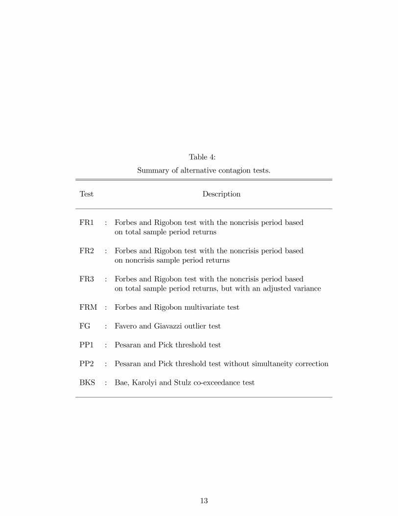
Table 4:

Summary of alternative contagion tests.

Test Description

FR1 : Forbes and Rigobon test with the noncrisis period basedon total sample period returns

FR2 : Forbes and Rigobon test with the noncrisis period basedon noncrisis sample period returns

FR3 : Forbes and Rigobon test with the noncrisis period basedon total sample period returns, but with an adjusted variance

FRM : Forbes and Rigobon multivariate test

FG : Favero and Giavazzi outlier test

PP1 : Pesaran and Pick threshold test

PP2 : Pesaran and Pick threshold test without simultaneity correction

BKS : Bae, Karolyi and Stulz co-exceedance test

13

statistic makes use of the Fisher transformation to improve the asymptotic approximation

(Kendall and Stuart, Vol.1, p.390-391). Under the null hypothesis of no contagion from

country i to country j, νy = ρz, and

FR1d−→ N (0, 1) . (18)

4.2 Alternative Forbes and Rigobon Tests (FR2,FR3)

An alternative to the Forbes and Rigobon test (FR1) , is to model the noncrisis period using

just the non-crisis returns, namely xi,t. The test statistic is now obtained by replacing zi,t in

(16) by xi,t

FR2 =

12ln³1+νy1−νy

´− 1

2ln³1+ρx1−ρx

´q

1Ty−3 +

1Tx−3

, (19)

where bνy = bρyr1 +

³s2y,i−s2x,i

s2x,i

´ ¡1− bρ2y¢ , (20)

bρx is the estimator of the correlation coefficient ρx = Corr (xi,t, xj,t), and s2x,i is the sample

variance corresponding to σ2x,i. Under the null hypothesis of no contagion from country i to

country j, νy = ρx, and

FR2d−→ N (0, 1) . (21)

An advantage of using FR2 is that the assumption of independence between the crisis

and noncrisis samples is satisfied. This is not the case with the FR1 statistic where the

noncrisis period is defined as the total sample period. For this case the correct asymptotic

variance is given by

V ar (bνy − bρz) = V ar (bνy) + V ar (bρz)− 2Cov (bνy,bρz)= V ar (bνy) + V ar (bρz)− 2V ar (bρz)= V ar (bνy)− V ar (bρz)=

1

Ty− 1

Tz, (22)

where the second and third steps are based on the result Cov (bνy,bρz) = V ar (bρz) ,5 whilstthe last step uses the result that for iid normal samples the asymptotic approximation of

5Let ut and vt be two iid random variables. Define the first and second sub-samples as T1 and T2, and

14

the variance of the correlation coefficient is given by the inverse of the sample size (Kendall

and Stuart (1973, p.307)). All details are given in the Appendix. Using (22) in (16) yields

a third version of the Forbes and Rigobon test statistic

FR3 =

12ln³1+νy1−νy

´− 1

2ln³1+ρz1−ρz

´q

1Ty−3 − 1

Tz−3. (23)

As the variance of FR3 is smaller than FR1 in (16), the latter statistic is expected to yield

smaller values on average resulting in this test being biased towards not rejecting the null of

no contagion.

4.3 Forbes and Rigobon Multivariate Test (FRM)

Dungey, Fry, González-Hermosillo and Martin (2005b) show that an alternative to the

Forbes-Rigobon test is to perform a Chow structural break test using dummy variables,

where the dependent and independent variables are scaled by the respective noncrisis stan-

dard deviations. One advantage of this formulation is that it provides a natural extension of

the bivariate approach to a multivariate framework that jointly models and tests all combi-

nations of contagious linkages. A further advantage is that it is computationally more easy

to implement than the multivariate extension based on the DCC test proposed by Rigobon

(2003).

The Forbes and Rigobon multivariate contagion test investigated here is based on the

the total sample period as T . The covariance between xt and yt over the total sample period is

Cov (xt, yt) =1

T

TXt=1

(xt − x) (yt − y)

=1

T

ÃTXt=1

(xt − x) (yt − y) +TXt=1

(xt − x) (yt − y)

!

=1

T

ÃT1Xt=1

(xt − x) (yt − y) +TX

t=T1+1

(xt − x) (yt − y)

!

=T1TCov (xt, yt)1 +

T2TCov (xt, yt)2

where Cov (xt, yt)i is the covariance between xt and yt for sub-period i = 1, 2. Because of independence

15

following set of regression equationsµz1,tσx,1

¶= α1,0 + α1,ddt + α1,2

µz2,tσx,2

¶+ α1,3

µz3,tσx,3

¶+γ1,2

µz2,tσx,2

¶dt + γ1,3

µz3,tσx,3

¶dt + η1,t

µz2,tσx,2

¶= α2,0 + α2,ddt + α2,1

µz1,tσx,1

¶+ α2,3

µz3,tσx,3

¶(24)

+γ2,1

µz1,tσx,1

¶dt + γ2,3

µz3,tσx,3

¶dt + η2,t

µz3,tσx,3

¶= α3,0 + α3,ddt + α3,1

µz1,tσx,1

¶+ α3,2

µz2,tσx,2

¶+γ3,1

µz1,tσx,1

¶dt + γ3,2

µz2,tσx,2

¶dt + η3,t,

where

dt =

½1 : t > Tx0 : otherwise

, (25)

represents a crisis dummy variable and ηi,t are disturbance terms. Tests of contagion amount

to testing the significance of the parameters γi,j. For example, to test for contagion from

country 1 to country 2 the null hypothesis is γ2,1 = 0. It is also possible to perform joint

tests such as testing contagion from country 1 to both countries 2 and 3. The null hypothesis

in this case is γ2,1 = γ3,1 = 0.

4.4 Favero and Giavazzi Outlier Test (FG)

The Favero and Giavazzi (2002) test is similar to the multivariate version of the Forbes

and Rigobon test in (24) as both procedures amount to testing for contagion using dummy

variables. The FG approach consists of two stages: (a) Identification of outliers using a VAR;

(b) Estimation of a structural model that incorporates the outliers of the previous step using

dummy variables. The dummy variables are defined as

di,t =

½1 : |vi,t| > 3σv,i0 : otherwise

(26)

where there is a unique dummy variable corresponding to each outlier, and vi,t are the

residuals from a VAR that contains the asset returns of all variables in the system with

respective variances σ2v,i. That is, a dummy variable is constructed each time an observation

is judged extreme, |vi,t| > 3σv,i, with a one placed in the cell corresponding to the point

16

in time when the extreme observation occurs, and zero otherwise. Let d1,t, d2,t and d3,t,

represent the idiosyncratic sets of dummy variables for countries 1 to 3 respectively, and

dc,t, be the set of dummy variables that are classified as common to all asset markets ie the

dummy variables that are equivalent. This last feature of the model is needed to circumvent

multicollinearity problems from using two equivalent variables.

The next stage of the Favero and Giavazzi framework is to specify the following structural

model containing the dummy variables over the full sample period

z1,t = α1,0 + α1,2z2,t + α1,3z3,t + θ1z1,t−1

+γ1,1d1,t + γ1,2d2,t + γ1,3d3,t + γ1,cdc,t + η1,t

z2,t = α2,0 + α2,1z1,t + α2,3z3,t + θ2z2,t−1 (27)

+γ2,1d1,t + γ2,2d2,t + γ2,3d3,t + γ2,cdc,t + η2,t

z3,t = α3,0 + α3,1z1,t + α3,2z2,t + θ3z3,t−1

+γ3,1d1,t + γ3,2d2,t + γ3,3d3,t + γ3,cdc,t + η3,t,

where ηi,t are structural disturbance terms. The γi,j are vectors of parameters in general,

with dimensions corresponding to the number of dummy variables in d1,t, d2,t, d3,t and dc,t.

Treating the dummy variables as predetermined, this model is just identified and can be

conveniently estimated by FIML using an instrumental variables estimator. The instruments

chosen are the three lagged returns, the constant and all dummy variables. Tests of contagion

are based on testing the γi,j ∀i 6= j parameters.

4.5 Pesaran and Pick Threshold Test (PP1)

The Pesaran and Pick (2004) contagion test is similar to the approach of Favero and Giavazzi

(2002) as both involve identifying outliers initially and then using these outliers in a structural

model to test for contagion. One important difference between the two approaches is that

Pesaran and Pick do not define a dummy variable for each outlier, but combine the outliers

associated with each variable into a single dummy variable. This is equivalent to restricting

the parameters on the Faverro and Giavazzi dummy variables to be equal.

17

The specification of the dummy variable for the ith asset return is given by6

di,t =

½1 : |vi,t| > τ i0 : otherwise

, (28)

where vi,t i = 1, 2, 3, are the residuals from a VAR that contains the asset returns of all

variables in the system, and τ i is a threshold which picks out the biggest 10% of outliers in

asset return i.7

The structural model is specified as

z1,t = β1,0 + θ1z1,t−1 + γ1,2d2,t + γ1,3d3,t + η1,t

z2,t = β2,0 + θ2z2,t−1 + γ2,1d1,t + γ2,3d3,t + η2,t (29)

z3,t = β3,0 + θ3z3,t−1 + γ3,1d1,t + γ3,2d2,t + η3,t,

where ηi,t are structural disturbance terms. Unlike Favero and Giavazzi, Pesaran and Pick

treat the dummy variables as endogenous. A further difference in the two approaches is that

Pesaran and Pick do not include own dummy variables, whereas Favero and Giavazzi do. The

structural model in (29) is just identified and can be conveniently estimated by FIML using

an instrumental variables estimator. The instruments chosen are the three lagged returns,

and the constant. Tests of contagion are based on testing the parameters γi,j, ∀i 6= j.

4.6 Adjusted Pesaran and Pick Threshold Test (PP2)

An alternative version of the Pesaran and Pick contagion test investigated in the Monte

Carlo experiments is to estimate (29) by OLS and not adjust for any simultaneity bias. This

form of the test is motivated by the possibility of weak instruments and its consequences for

testing for contagion. These issues are discussed further below.

6Other choices of the switch point of the dummy variable could be based on the approach of Faveroand Giavazzi (2002) in (26), or the exchange market pressure index used by Eichengreen, Rose and Wyplosz(1995, 1996). Baur and Schulze (2002) consider an endogenous approach, while Bae, Karolyi and Stulz (2003)adopt an asymmetric approach and consider positive and negative extreme returns separately. The approachadopted here has the advantage that it circumvents potential problems in the simulations conducted belowwhen no outliers are detected.

7Pesaran and Pick do not control for common factors by using a VAR. However, for commensurabilitythis will be adopted in the simulation framework below.

18

4.7 Bae, Karolyi and Stulz Co-exceedance Test (BKS)

The co-exceedance test of Bae, Karolyi and Stulz (2003) is also based on the dummy variable

expression in (28) to identify periods of contagion. An important difference between the BKS

approach and the Pesaran and Pick approach however, is that the dependent variable is also

transformed to a dummy variable.

In the BKS framework, the dummy variables are commonly referred to as exceedances.

Two versions of the BKS framework are considered. The first is based on a trivariate frame-

work where the aim is to perform a joint test of contagion from country 1 to countries 2 and

3. Define the polychotomous dummy variable between the returns of countries 2 and 3, as

e2,3,t =

⎧⎪⎪⎨⎪⎪⎩0 : d2,t = 0 and d3,t = 01 : d2,t = 1 and d3,t = 02 : d2,t = 0 and d3,t = 13 : d2,t = 1 and d3,t = 1

. (30)

Points in time when both countries 2 and 3 experience extreme returns, e2,3,t = 3, are referred

to as co-exceedances. Associated with each value of the polychotomous dummy variable e2,3,t,

is a probability

pj,t = Pr (e2,3,t = j) , j = 0, 1, 2, 3.

To test for contagion, the following multinomial logit model is estimated by maximum

likelihood where the probabilities are parameterized by the logistic function

pj,t =exp

¡μj + γjd1,t

¢Σ3k=0 exp

¡μj + γjd1,t

¢ , j = 0, 1, 2, 3, (31)

where the restriction μ0 = γ0 = 0, is chosen as the normalization. The inclusion of the

dummy variable d1,t, from (28), represents the extreme returns of country 1, and forms

the basis of the contagion tests from this country to the other two countries. The test of

contagion from country 1 to country 2 is based on testing that γ1 = 0. For non-zero values

of γ1, extreme returns in country 1 impact upon returns in country 2. To test for contagion

from country 1 to country 3, the pertinent restriction to be tested is γ2 = 0. A joint test

of contagion from country 1 to countries 2 and 3, is given by testing the restriction γ3 = 0,

as a non-zero value of γ3 corresponds to where extreme shocks in the returns of country 1

impact simultaneously on countries 2 and 3. To test for contagion in other directions, d1,t is

replaced by a dummy variable representing extreme returns of another country, and e2,3,t in

(30) is appropriately redefined.8

8Another way to perform bidirectional tests of contagion is to define the polychotomous dummy variable

19

4.8 Discussion

4.8.1 Biasedness in Testing for Contagion Using Correlations

An important feature of the FR2 test is that it is based on testing the difference in bivariate

correlations between noncrisis and crisis periods. Using the expressions for the variance-

covariance matrices in (10) and (11), the difference in the two correlations between countries

1 and 2 is immediately given by

ρy1,t,y2,t − ρx1,t,x2,t =λ1λ2ω

2 + δ2φ21p

λ21ω2 + φ21

pλ22ω

2 + φ22 + δ22φ21

− λ1λ2pλ21 + φ21

pλ22 + φ22

. (32)

Some insight into this expression is obtained by looking at what happens as the strength

of contagion continuously increases (with δ2 replaced by δ) and when there is no structural

break in the common factor (ω = 1)

limδ→∞

³ρy1,t,y2,t − ρx1,t,x2,t

´= lim

δ→∞

Ãλ1λ2 + δφ21p

λ21 + φ21pλ22 + φ22 + δ2φ21

!− λ1λ2p

λ21 + φ21pλ22 + φ22

= limδ→∞

⎛⎝ λ1λ2/δ + φ21pλ21 + φ21

qλ22/δ

2 + φ22/δ2 + φ21

⎞⎠− λ1λ2pλ21 + φ21

pλ22 + φ22

=1p

λ21 + φ21

Ãφ1 −

λ1λ2pλ22 + φ22

!. (33)

For relatively “high” levels of contagion, the correlation in the noncrisis period³ρx1,t,x2,t

´can exceed the crisis period correlation

³ρy1,t,y2,t

´when

φ1 −λ1λ2pλ22 + φ22

< 0,

or

1 +

µφ2λ2

¶2<

µλ1φ1

¶2. (34)

Thus the key magnitudes for determining the relative magnitudes of the correlations between

asset returns in the two sample periods, are the relative sizes of the loadings of the common

factor (λi) to the idiosyncratic factor (φi) for the two asset returns.

e2,3,t in (30), simply in terms of one variable; that is, define a binary dummy variable. This is also theapproach adopted by Eichengreen, Rose and Wyplosz (1995, 1996), except that they specify the underlyingdistribution to be normal, resulting in the use of a probit model.

20

Figure 3 gives the difference in the crisis correlation¡ρy¢and noncrisis correlation (ρx)

between selected pairs of countries based on (32) for alternative values of the contagion

parameter (δ = δ2 = δ3) and the structural break parameter (ω) , with the values of the

remaining parameters given by

λ1 = 4, λ2 = 2, λ3 = 3, φ1 = 2, φ2 = 10, φ3 = 4.

For the case where there is no structural break in the common factor (ω = 1) , Figure 3(a)

shows that the difference in the correlations between countries 1 and 2 increases monoton-

ically initially as δ increases and eventually flattens out to a difference of 0.3. This re-

sult is to be expected as the expression in (34) is not satisfied for this parameterization:

1 + (φ2/λ2)2 = 1 + (10/2)2 = 26 is greater than (λ1/φ1)

2 = (4/2)2 = 4.

Figure 3(b) gives the difference in correlations between countries 1 and 3 with country 2

replaced by country 3 in (32). Here an alternative pattern to the one presented in Figure 3(a)

emerges whereby the difference in correlations between countries 1 and 3 initially increases,

then starts to decrease and eventually becomes negative for contagion levels of δ > 15. For

this case the inequality in (34) is now satisfied as 1+(φ3/λ3)2 = 1+(4/3)2 = 2.778 is less than

(λ1/φ1)2 = (4/2)2 = 4. This result is at odds with the usual strategy of testing for contagion

based on identifying a significant increase in correlation during a crisis period. That is, the

null hypothesis is usually taken as one-sided when testing for contagion based on correlation

analysis; see also the discussion in Billio and Pelizzon (2003). However, this phenomenon is

not uncommon in applied work when computing the correlation structure of asset returns

during financial crises. What this result shows is that looking at simple correlations can

be highly misleading when attempting to identify evidence of contagion. Even though for

certain parameterization the correlation during the crisis period is less than it is for the

noncrisis period, Figure 3(b) highlights that this is not inconsistent with the presence of

contagion (δ > 0). From a testing point of view, this result also suggests that in testing for

contagion based on correlation analysis, the power of the test statistic to detect contagion

may not be monotonic over the parameter space. In fact, this test is not guaranteed to be

unbiased, especially for one-sided null hypotheses.9

In contrast to the FR2 test, the FR1 and FR3 tests are based on comparing the crisis

correlation with the total correlation. Defining the covariance and variance of the total9The phenonemon that noncrisis correlations can exceed crisis correlations also suggests that the practice

of choosing a crisis sample on the basis of the correlation in the crisis period exceeds the correlation in thenon-crisis period is clearly inappropriate.

21

Figure 3: Differences in the crisis and pre-crisis correlations for alternative values of thecontagion parameter (δ = δ2 = δ3) and the structural break parameter (ω) .

period to be weighted averages of the crisis and noncrisis analogues, the expression in (32)

is now replaced by³ρy1,t,y2,t − ρz1,t,z2,t

´=

λ1λ2 + δφ21pλ21 + φ21

pλ22 + φ22 + δ2φ21

− λ1λ2Tx/T +¡λ1λ2 + δφ21

¢Ty/T

ζ, (35)

where

ζ =q¡

λ21 + φ21¢Tx/T +

¡λ21 + φ21

¢Ty/T

q¡λ22 + φ22

¢Tx/T +

¡λ22 + φ22 + δ2φ21

¢Ty/T

and Tx and Ty are, as before, respectively the sample sizes of the noncrisis and crisis periods,

and T = Tx + Ty is the total sample period. Taking the limit as δ →∞, yields

limδ→∞

³ρy1,t,y2,t − ρz1,t,z2,t

´=

φ1pλ21 + φ21

Ã1−

rTyT

!> 0.

Unlike the expression for limδ→∞³ρy1,t,y2,t − ρx1,t,x2,t

´in (33), the difference in the correla-

tions is now guaranteed to be positive. This expression shows that as the relative proportion

of the crisis period to the total period increases, the difference in the two correlations de-

creases. In the limit there would be no difference in the two correlations as the total and

crisis periods would be the same. Figure 4 demonstrates the properties of (35) for the same

parameterization used in Figure 3. In Figure 4(a) the difference in correlations is monotonic

in δ initially, reaching a threshold for δ > 5. In contrast, the pattern presented in Figure

4(b) is not monotonic for all values of δ, but is nonetheless still positive.

22

Figure 4: Differences in the crisis and total crisis correlations for alternative values of thecontagion parameter (δ = δ2 = δ3) and the structural break parameter (ω) .

4.8.2 Spuriousness in Testing for Contagion

Contagion tests based on bivariate analysis such as the Forbes and Rigobon tests (FR1 and

FR2), can potentially yield spurious contagious linkages between variables as a result of

a common factor. This point is highlighted in Figure 5(a) in particular, which gives the

difference in the crisis and noncrisis correlations between countries 2 and 3 for alternative

values of the contagion parameter (δ = δ1 = δ2) and the structural break parameter (ω) . As

the strength of contagion increases (δ > 0) , the correlation between the two asset returns

increases. This increase in correlation is purely spurious as it arises from both variables

being affected by a common factor, namely shocks from country 1 asset returns. A similar

property is presented in Figure 5(b) which compares the crisis and total correlations between

countries 2 and 3.

4.8.3 Structural Breaks

Loretan and English (2000) and Forbes and Rigobon (2002) emphasize the problems of

structural breaks in testing for contagion. The problem is highlighted in Figures 3 to 5 for

the case of a structural break in the common factor (ω > 1). Increases in the strength of the

structural break accentuates the differences in the noncrisis and crisis correlations. Figure

3(a) also shows that for greater levels of contagion, the switch in the magnitudes of the

correlations in the two sample periods becomes even more marked.

23

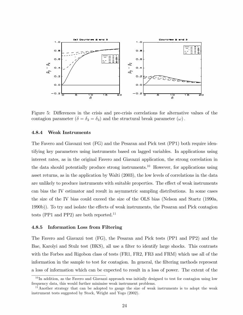
Figure 5: Differences in the crisis and pre-crisis correlations for alternative values of thecontagion parameter (δ = δ2 = δ3) and the structural break parameter (ω) .

4.8.4 Weak Instruments

The Favero and Giavazzi test (FG) and the Pesaran and Pick test (PP1) both require iden-

tifying key parameters using instruments based on lagged variables. In applications using

interest rates, as in the original Favero and Giavazzi application, the strong correlation in

the data should potentially produce strong instruments.10 However, for applications using

asset returns, as in the application by Walti (2003), the low levels of correlations in the data

are unlikely to produce instruments with suitable properties. The effect of weak instruments

can bias the IV estimator and result in asymmetric sampling distributions. In some cases

the size of the IV bias could exceed the size of the OLS bias (Nelson and Startz (1990a,

1990b)). To try and isolate the effects of weak instruments, the Pesaran and Pick contagion

tests (PP1 and PP2) are both reported.11

4.8.5 Information Loss from Filtering

The Favero and Giavazzi test (FG), the Pesaran and Pick tests (PP1 and PP2) and the

Bae, Karolyi and Stulz test (BKS), all use a filter to identify large shocks. This contrasts

with the Forbes and Rigobon class of tests (FR1, FR2, FR3 and FRM) which use all of the

information in the sample to test for contagion. In general, the filtering methods represent

a loss of information which can be expected to result in a loss of power. The extent of the

10In addition, as the Favero and Giavazzi approach was initially designed to test for contagion using lowfrequency data, this would further minimise weak instrument problems.11Another strategy that can be adopted to gauge the size of weak instruments is to adopt the weak

instrument tests suggested by Stock, Wright and Yogo (2002).

24

loss in power is investigated in Monte Carlo experiments conducted below.

5 Finite Sample Properties

This section presents the finite sample properties of the eight contagion tests using a number

of Monte Carlo experiments. The experiments are conducted to identify the size and power

properties of the test statistics under various scenarios, including autocorrelation, structural

breaks, GARCH conditional variance and unknown crisis periods.

5.1 Experimental Design

The DGP used in the Monte Carlo experiments is an extension of the DGP discussed in

Section 3 by allowing for different types of structural breaks, autocorrelation in the common

factor as well as time varying volatility based on a GARCH conditional variance. The model

consists of three asset returns during a noncrisis period (x1,t, x2,t, x3,t) and a crisis period

(y1,t, y2,t, y3,t) . The crisis period is characterized by contagion from y1,t to both y2,t, and y3,t.

The crisis period also allows for structural breaks in the common factor (wt) and or the

idiosyncratic factor of y1,t.

Non-crisis Model

x1,t = 4wt + 2u1,t (36)

x2,t = 2wt + 10u2,t (37)

x3,t = 3wt + 4u3,t, (38)

where

wt = ρwt−1 + uw,t (39)

uw,t ∼ N (0, ht) (40)

ht = ω2¡1− α− β + αu2w,t−1 + βht−1

¢(41)

ui,t ∼ N (0, 1) i = 1, 2, 3. (42)

Crisis Model

y1,t = 4wt + 2u1,t (43)

y2,t = 2wt + 10u2,t + δ2u1,t (44)

y3,t = 3wt + 4u3,t + δ2u1,t, (45)

25

where

wt = ρwt−1 + uw,t (46)

uw,t ∼ N (0, ht) (47)

ht = ω2¡1− α− β + αu2w,t−1 + βht−1

¢(48)

u1,t ∼ N¡0, κ2

¢(49)

ui,t ∼ N (0, 1) i = 2, 3. (50)

The strength of contagion is controlled by the parameter δ in (44) and (45), with para-

meter values set at

δ = 0, 1, 2, 5, 10 . (51)

A value of δ = 0, represents no contagion and is used to examine the size properties of the

test statistics in small samples when the asymptotic critical values are used. Values of δ > 0,

are used to examine the power properties of the contagion tests using size-adjusted critical

values.

Two types of structural breaks are investigated. The first is a structural break in the

common factor wt. The parameter values chosen are

ω = 1, 5 , (52)

where ω = 1, represents no structural break in the common factor during the crisis period.

The second is a structural break in the idiosyncratic factor of y1,t, namely u1,t. The parameter

values are

κ = 1, 5 , (53)

where κ = 1, represents no structural break in the idiosyncratic factor during the crisis

period.

The parameters α and β allow for a time varying volatility GARCH process common in

financial market data. In the case where there is no conditional volatility

α = β = 0.

For the conditional volatility case the parameters are set at

α = 0.05, β = 0.90,

26

which are typical parameter estimates reported in empirical studies of financial returns (En-

gle, (2004)).

Eight Monte Carlo experiments are performed which are summarized in Table 5. For

each experiment, six hypotheses are tested (Table 6) using eight alternative contagion tests

(Table 4). The FR1, FR2 and FR3 tests are used to test the first four hypotheses in Table

6, but not the two joint hypotheses as these tests are bivariate by construction. The BKS

test is not used to test the last joint hypothesis in Table 6 as this would involve stacking

three sets of multivariate log likelihoods.

5.2 Computational Issues

All test statistics are based on a preliminary step consisting of extracting the residuals from

estimating a trivariate VAR for z1,t, z2,t, z3,t with one lag over the full sample period.The Forbes and Rigobon set of univariate contagion tests (FR1, FR2, FR3) are evaluated

by replacing zi,t in the pertinent formulae by the VAR residuals. This preliminary step is

motivated by the empirical strategy adopted by Forbes and Rigobon (2002) who use it as a

way of extracting out any common factors in the data.

The multivariate version of the Forbes and Rigobon test (FRM) is also obtained by

replacing zi,t in (24) by the VAR residuals and estimating the set of equations by OLS. The

FRM contagion test is evaluated using a Wald statistic.

The VAR residuals are used to compute the Favero and Giavazzi set of dummy variables

defined in (26), which, in turn, are used in the structural model (27). This set of equations

is estimated by IV which is asymptotically equivalent to FIML as the system of equations

is just identified. Following the empirical work of Favero and Giavazzi, the contagion test

(FG) is based on a likelihood ratio test.

The Pesaran and Pick contagion tests (PP1 and PP2) use the VAR residuals to compute

the dummy variables in (28) which are used in the structural model in (29). The PP1 test

is based on estimating the structural model by an IV estimator with the set of instruments

consisting of a constant and all lagged variables Const, z1,t−1, z2,t−1, z3,t−1 . The PP2 testis obtained by ignoring potential simultaneity bias and replacing the IV estimator by the

OLS estimator. Both contagion tests are evaluated using a Wald statistic.

The BKS contagion test (BKS) is based on using the VAR residuals to compute the

exceedances and co-exceedances in (30). The BKS statistic is evaluated by estimating the

27

Table 5:

Summary of the Monte Carlo experiments.

Experiment Type Restrictions Crisis Period

I Strong Autocorrelation ω = 1, κ = 1, ρ = 0.95, Knownα = 0.0, β = 0.0

II Weak Autocorrelation ω = 1, κ = 1, ρ = 0.2, Knownα = 0.0, β = 0.0

III No Autocorrelation ω = 1, κ = 1, ρ = 0.0, Knownα = 0.0, β = 0.0

IV Idiosyncratic structural break ω = 1, κ = 5, ρ = 0.0, Knownα = 0.0, β = 0.0

V Common structural break ω = 5, κ = 1, ρ = 0.0, Knownα = 0.0, β = 0.0

VI Common structural break ω = 5, κ = 1, ρ = 0.0, KnownGARCH conditional variance α = 0.05, β = 0.95

VII Idiosyncratic structural break ω = 1, κ = 5, ρ = 0.0, Unknownα = 0.0, β = 0.0

VIII Common structural break ω = 5, κ = 1, ρ = 0.0, Unknownα = 0.0, β = 0.0

28

Table 6:

Hypotheses tested in the Monte Carlo experiments.

Test Hypothesis

y1,t → y2,t H0 : γ2,1 = 0y1,t → y3,t H0 : γ3,1 = 0y2,t → y3,t H0 : γ3,2 = 0y3,t → y2,t H0 : γ2,3 = 0

y1,t → y2,t, y3,t H0 : γ2,1 = γ3,1 = 0

y1,t → y2,t, y3,ty2,t → y3,ty3,t → y2,t

H0 : γ2,1 = γ3,1 = γ3,2 = γ2,3 = 0

system of equations in (31) by MLE. The BFGS algorithm in GAUSS is used to maximize the

likelihood, with the maximum number of iterations set at 200. This is a gradient algorithm

with the derivatives computed numerically.12

In the case where the crisis period is known, the Forbes and Rigobon tests (FR1, FR2,

FR3, FRM) use all of the information in the crisis period to compute crisis correlations and

define dummy variables as is needed in the case of the FRM test. The threshold dummy

variables defined in (26) for the FG test are identified as the largest 5% of values during the

crisis period. The same rule is adopted in (28) for the PP1 and PP2 tests. The exceedances

and co-exceedances in (30) for the BKS tests are identified as the largest 10% of values

during the crisis period.

In the experiments where the crisis period is unknown the rules for each of the tests are

chosen as follows. The crisis period for the Forbes and Rigobon tests is selected as points

in time corresponding to the largest observation in all returns. To avoid choosing a break

point to close to the boundaries of the data, the first and last ten observations are excluded

from identifying the start of the crisis period. The FG crisis period is determined by the

12The use of a VAR to extract out the dependence structure in the data is problematic in the case of theBKS approach which uses a multivariate logit model based on the assumption that the dichotomous variablesare independent, although not identical. To introduce dependence directly into the model through eitherthe mean (autocorrelation) or the variance (GARCH), would yield a more complicated likelihood functionwhich would make estitmation more complicated.

29

rule given in (26). The PP crisis period is determined by the rule given in(28). Finally, the

BKS crisis period is identified by the exceedances and co-exceedances as defined in (30).

In computing the size and power of the FG test in the case of the crisis sample period

being unknown, the critical value will change in each draw of the Monte Carlo experiment as

the number of outliers and hence the number of dummy variables that are being tested will

change. To compute the size and power in this case the approach adopted is to perform the

test using the asymptotic critical value from a chi-squared distribution where the degrees of

freedom equalled the number of dummy variables being tested. The size and power are then

simply computed as the sample mean of the number of times the null is rejected. In the ex-

periments where the sample size is known (Experiments I to VI) the asymptotic distribution

is simply χ25 as the number of extreme observations is always set at 5 by construction.

All Monte Carlo experiments are conducted in Gauss 6.0, with each experiment based on

10, 000 replications. The normal random numbers are generated using the GAUSS procedure

RNDN, with a seed equal to 123457. The noncrisis sample size is set at Tx = 100, while the

sample for the crisis period is chosen as Ty = 50.

5.3 Size

The finite sample results of the size of the eight contagion tests across the eight experiments,

are presented in Table 7 (Experiments I to IV) and Table 8 (Experiments V to VIII). Figures

6 and 7 gives the full sampling distributions across the eight experiments for each test in

the case of testing the hypothesis of contagion form y1,t to y2,t.13 The results are based on

simulating the model under the null hypothesis of no contagion by setting δ = 0. The sizes

are based on the 5% (one-sided) asymptotic normal critical values in the case of the FR1,

FR2 and FR3 tests, while the sizes of the remaining test statistics are based on the 5%

asymptotic chi-squared critical values.

The sampling distributions of the FR1, FR2 and FR3 test statistics under the null hy-

pothesis of no contagion are given in the top nine panels of Figure 6 for testing y1,t → y2,t.

For comparison, the asymptotic distribution, N (0, 1) , is also presented. The part of the

right tail of the sampling distribution of the FRM test statistic is given in the bottom three

panels of Figure 6 to test the same hypothesis, while Figure 7 contains the tails of the sam-

13The reported sampling distributions are based on a normal kernel with the bandwidth computed usinga normal reference rule in the case of FR1, FR2 and FR3. For the remaining tests, the sampling distributionis based on a logarithmic transformation kernel to ensure postivity of the sampling distribution.

30

pling distribution of the FG, PP1, PP2 and BKS test statistics. The asymptotic distribution

also included in the figures of the FRM, PP1, PP2 and BKS statistics for comparison is the

χ21 distribution, whereas for the FG statistic it is the χ25 distribution.

14

The FR1 statistic is consistently undersized (less than 0.050) for all experiments with the

test not rejecting the null of no contagion often enough. The problem is especially acute for

Experiments IV to VIII where there is a structural break in one of the factors. This feature

is highlighted in Figure 6 for the case of testing contagion from y1,t to y2,t.

The poor size properties of the FR1 statistic in the case of Experiments I to III, stem

from using an asymptotic variance based on incorrectly assuming independence between the

crisis and noncrisis (total in this case) samples. This point is highlighted in Figure 6 for

Experiments I to III, where the FR2 and FR3 test statistics generate sampling distributions

that closely approximate the asymptotic distribution. Table 7 shows that both of these tests

consistently yield sizes close to 0.05 for the first three experiments for all types of hypotheses

tested.

The FR1 and FR3 tests also exhibit low sizes in the presence of structural breaks. The

FR2 test also yields low sizes in the case of idiosyncratic structural breaks (Experiments IV

and VII), but reasonable sizes when structural breaks occur in the common factor. This

is true for when the crisis period is known (Experiment IV), there is GARCH conditional

volatility (Experiment VI) and the crisis period is unknown (Experiment VIII). This result

suggests that by splitting up the sample into two distinct sub-periods and not defining the

noncrisis period as the total period, provides a more robust test of contagion.

The FRM test also demonstrates good size properties for a range of experiments and

hypotheses tested, especially for the first three experiments. The bottom panels of Figure 6

show that the tails of the sampling distribution for these three experiments are close to the

right tail of the asymptotic sampling distribution (χ21). The size of FRM generally tends to

be slightly inflated compared to the sizes of FR2 and FR3, which reflects an efficiency loss

in conducting the FRM test in small samples as a result of the inclusion of variables that

are not part of the DGP. In contrast to the FR1, FR2 and FR3 tests, the FRM statistic

appears to be relatively robust to structural breaks, common or idiosyncratic, for most of

the hypotheses investigated, but not all. An exception is in testing for contagion from y1,t

to y3,t in Experiment IV, where the size of the test is inflated in excess of 0.95.

14The sampling distribution of the FG statistic is χ25, in the case where the crisis period is known (Ex-periements I to VI), while in the case where the crisis period is unknown it is a mixture of χ2 distributions.

31

The FG test is consistently oversized for all experiments and across all hypotheses tested.

The top three panels of Figure 7 highlight the fatness in the tails of the sampling distribution

in the case of testing the first hypothesis, namely contagion from y1,t to y2,t. Comparing the

sizes of the FG statistic across Experiments I to III, shows that the sizes increase as the level

of autocorrelation is reduced. This highlights the weak instrument problems with this test

as a reduction in autocorrelation leads to a deterioration in the quality of the instruments

yielding sampling distributions with fatter tails. In the extreme case where there is no

autocorrelation (Experiment III), the simultaneous equations model underlying the FG test

is underidentified and the instruments are now irrelevant.

A feature of the size properties of the PP1 statistic is that it is consistently undersized.

The thinness in the tails of the distribution are highlighted in Figure 7 for the case of the

first hypothesis being tested, with the tails of all experiments lying below the tail of the

asymptotic distribution. This result is in stark contrast to the size properties of the FG

test which is consistently oversized, but in agreement with the FR1 statistic which is also

consistently undersized in all experiments. The poor size properties of the test reflects the

loss of information in modelling contagion through the specification of dummy variables. This

loss of information would appear to be particularly severe as this effect is able to dominate

the weak instrument effect which could have the opposite result of inflating the size of the

statistic. This point is highlighted by looking at the size properties of the PP2 test statistic.

As this statistic uses more information than PP1, its size properties should be marginally

better. This is true in the case of Experiment I, but for all other experiments the sizes are

practically the same as they are for PP1.

The size properties of the BKS statistic are similar to the FG statistic as it also yields

relatively inflated sizes across most experiments and across most hypotheses. An exception

is in Experiment VII where the sizes are reasonable, ranging between 0.039 to 0.095 for all

of the four single tests of contagion.

5.4 Power

Tables 9 to 16 give the probability of finding contagion, adjusted by size, for each of the eight

tests for increasing intensity levels of contagion, δ = 1, 2, 5, 10, across the eight experiments.

As contagion is assumed to run from y1,t to both y2,t and y3,t during the crisis period, the

power of the test should increase monotonically as δ increases for the first two hypotheses,

32

y1,t → y2,t and y1,t → y3,t. For the third and fourth hypotheses, y2,t → y3,t and y3,t → y2,t,

the power should be equal to the size adjusted value of the test, namely 0.05. Although the

size of the FR3 test is closer to the asymptotic distribution under the null than FR1, the

power functions of the FR1 and FR3 tests are identical as the use of the size adjusted critical

values merely rescales the relevant distributions.

5.4.1 Autocorrelation: Experiments I to III

Tables 9 to 11 give the size adjusted power functions for the alternative contagion tests for

high (Table 9), low (Table 10) and zero (Table 11) levels of autocorrelation. In testing for

contagion from y1,t to y2,t and y3,t, the FR1 and FR3 tests both exhibit monotonic power

functions with the power of the test increasing for increasing levels of autocorrelation. The

FR2 test exhibits slightly better power in testing for contagion from y1,t to y2,t, but its power

function is non-monotonic in testing for contagion from y1,t to y3,t. This latter result reflects

the properties of the correlation function presented in Figure 3(b), where it is revealed that

the correlation between two series can decrease for relatively high levels of contagion and

even become negative. The FR2 and FRM tests exhibit similar power functions with the

latter test yielding marginally inferior power properties.

Tables 9 to 11 reveal that the remaining tests (FG, PP1, PP2 and BKS) all exhibit

very low and flat power functions in testing for contagion from y1,t to y2,t and y3,t. To try

and unravel the poor performance of these tests a comparison of the PP1 and PP2 reveals

approximately a 100% improvement in power in testing for contagion from y1,t to y2,t and

y3,t, for high levels of autocorrelation (Table 9). This result is interpreted as a problem

of weak instruments with the PP1 test with the bias arising from using weak instruments

(PP1) exceeding the simultaneity bias (PP2). However, as the strength of autocorrelation

falls (Tables 10 and 11), the improvement in power between PP1 and PP2 tapers off with

the powers of the two tests tending to converge for the extreme case where there is no

autocorrelation (Table 11). One way to understand this result is to compare the power

properties of the PP2 test with the power of FRM test, which also does not correct for

potential simultaneity bias. The main difference in the two tests is how contagion is identified.

With the PP2 test only “big” shocks are included whereas with the FRM test all shocks are

included in testing for contagion. The reduction in power of the PP2 test then represents

the information loss of using a filter that excludes important sample information.

While a comparison of the power properties of the FR1, FR2 and FR3 in testing the

33

first two hypotheses reveals that the FR2 exhibits slightly better power, this comes at a cost

in testing for contagion between y2,t and y3,t, where the test incorrectly identifies contagion

with the probability of detection increasing as the strength of contagion increases. The

power functions of the FR1 and FR3 tests corresponding to these two hypotheses exhibit

non-monotonic functions with the power first increasing and then decreasing for higher levels

of contagion.

5.4.2 Structural Breaks: Experiments IV to VI

The size adjusted power functions of alternative tests of contagion are given in Table 12

(idiosyncractic structural break), Table 12 (common structural break) and Table 14 (common

structural break with conditional volatility).

Table 12 shows that the bivariate FR tests (FR1, FR2 and FR3) all exhibit high power

in testing contagion in the presence of idiosyncractic structural breaks from y1,t to y2,t and

y3,t, with power quickly approaching unity for even “moderate” levels of contagion in most

cases. In contrast, all remaining contagion tests exhibit low power with at best, very flat

power functions across the contagion spectrum.

Table 12 also shows that the power in testing for contagion between y2,t and y3,t using

the FR1 and FR2 tests incorrectly yield a probability in excess of 0.05 of finding contagion

for “low” levels of contagion, but this probability falls as the strength of contagion increases

and approaches the correct level of 0.05 for “large” values of contagion. In contrast, the FR2

and FRM tests incorrectly find contagion between y2,t and y3,t and that the power function

quickly approaches unity for the FRM test, especially in testing for contagion from y2,t to

y3,t. This result suggests that by choosing the noncrisis period as the total period (FR1 and

FR3) yields a more robust test of contagion especially in the case where there are structural

breaks in the idiosyncratic factor. Of course, the Forbes and Rigobon test is designed to

capture idiosyncratic structural breaks by using the adjusted correlation coefficient given in

(17). In regards to the other tests of contagion, especially FG, PP1 and PP2, whilst these

tests yield powers close to the theoretical value of 0.05, this is simply the result of these

tests exhibiting very little power for any hypothesis test at any level of contagion in the first

place.

Table 13 shows that all tests have low power in the presence of a structural break in the

common factor. An exception is the FRM test which exhibits increasing power in testing for

contagion from y1,t and y2,t, however this test also incorrectly has increasing power in testing

34

for contagion between y2,t and y3,t. By allowing for a GARCH conditional variance in the

common factor (Table 14) does not change the power properties of the tests in the presence

of a structural break in the common factor.

5.4.3 Crisis Period Unknown: Experiments VII to VIII

The power properties of the contagion tests in the presence of idiosyncratic and common

structural breaks are given in Tables 15 and 16 respectively, when the crisis period is un-

known. Comparing these results with the respective power properties in Tables 12 and 13

where the crisis period is known, not surprisingly reveals that there is a slight loss of power

with the FR1, FR2 and FR3 tests. As in the case where the crisis period is known, the other

tests still exhibit low power.

5.4.4 Joint Tests of Contagion: Experiments I to VIII

The last two columns of Tables 9 to 16 give the power functions of two joint tests of contagion

for selected contagion tests. The first test is a test that there is contagion from y1,t to both

y2,t and y3,t, while the second test is a joint of overall contagion in all directions. The FRM

and BKS tests perform the best. The FRM test exhibits highest power for low and moderate

levels of contagion, but its power function begins to fall for high levels of contagion as a result

of the effects of the falling power detected in testing for contagion from y1,t to y3,t, discussed

previously. At this point in the power comparison, the BKS yields relatively higher power.

6 Conclusions

This paper has investigated the finite sample properties of a range of tests of contagion

commonly employed to detect propagation mechanisms during financial crises. The tests

investigated included the Forbes and Rigobon adjusted correlation test, the Favero and

Giavazzi outlier test, the Pesaran and Pick threshold test, and the Bae, Karolyi and Stulz

co-exceedance test. Some extensions of these tests were also proposed to adjust for size

distortions and weak instruments. The experiments conducted allowed for autocorrelation

in the mean and the variance, alternative types of structural breaks and situations where

the timing of the crisis period may either be known or unknown.

The results showed that the Forbes and Rigobon test is undersized. Two variants of this

test were proposed which were shown to correct the size distortion. The first adjustment

35

consisted of not defining the noncrisis period as the total period, while the second approach

involved deriving a new asymptotic standard error which took into account the lack of

dependence between the crisis and noncrisis periods as adopted in the original version of the

Forbes and Rigobon test. As with the original version of the Forbes and Rigobon test, the

Pesaran and Pick test was also undersized, whereas the Favero and Giavazzi test and the

Bae, Karolyi and Stulz test are oversized.

For certain parameterization some of the test statistics exhibited non-monotonic power

functions. This was shown to be less of a problem in the case of the Forbes and Rigobon

tests which defined the noncrisis period as the total sample. The Favero and Giavazzi test

and the Pesaran and Pick test exhibited low power which was the result of a combination

of weak instrument problems and, more importantly, a loss of information from the types

of filters employed in these tests to identify large shocks during crisis periods. The Bae,

Karolyi and Stulz also exhibited low power arising from the adoption of filters designed to

identify large shocks.

Most tests perform badly in terms of size and power in the presence of structural breaks.

One exception is the Forbes and Rigobon test where the noncrisis and crisis periods are

independent, which has reasonable size properties when there are idiosyncratic structural

breaks. Another exception is a multivariate version of the Forbes and Rigobon test pro-

posed by Dungey, Fry, González-Hermosillo and Martin, which tends to have reasonable size

properties for not only idiosyncratic structural breaks, but also common structural breaks.

The theoretical results of the paper have a number of important implications for under-

taking tests of contagion. First, the property that the Forbes and Rigobon test is undersized

is consistent with much of the empirical literature where empirical studies find little evidence

of contagion when using this test. A quick fix is either to define the crisis and noncrisis pe-

riods as disjoint samples, or if the noncrisis period is defined as the total sample period then

the correct asymptotic standard error, as derived in this paper, can be used.

Second, the Pesaran and Pick test is also undersized. This suggests that this test is also

a conservative test thereby it will tend not to find evidence of contagion when it does exist.

Third, and in contrast to the Forbes and Rigobon test and the Pesaran and Pick test,

the Favero and Giavazzi test and the Bae, Karolyi and Stulz test, are oversized. Again this

is consistent with the empirical findings where it is common to find evidence of contagion

when using these tests. This suggests that much of the empirical evidence of contagion using

36

these tests are potentially spurious, arising simply from adopting a test where the effective

probability of a Type I error is in excess of the usual level.

Fourth, when using the Favero and Giavazzi test and the Pesaran and Pick test, care

should be given to potential weak instrument problems. This is especially true for appli-

cations conducted on financial returns and the instruments chosen are the lagged returns.

One solution is to use a test that is robust to weak instruments (see Stock, Wright and Yogo

(2002) for a survey).

Fifth, care must be given to modelling structural breaks in testing for contagion otherwise

the tests can be badly biased. One solution is to use the multivariate version of the Forbes

and Rigobon test which was found to have the best robustness properties to the presence

of structural breaks. Another solution is to identify and model the timing of the structural

break before conducting a test of contagion (see Banerjee and Urga (2005) for a recent review

of structural break tests).

37

A Proof of the Asymptotic Variance of the AdjustedForbes and Rigobon Test

In this appendix, the standard error for the adjusted Forbes and Rigobon test is derived.

Let ry be the sample correlation for the second sample period (Ty), and r represent the

correlation for the total sample period (T = Tx + Ty) where Tx is the first sample period.

To construct a test of the difference in the second sub-sample and total correlations, it is

necessary to find

V ar (ry − r) = V ar (ry) + V ar (r)− 2Cov (ry, r) . (54)

Focussing on the last term

Cov (ry, r) = Cov

µm11√m20m02

,n11√n20n02

¶, (55)

where m11 (n11) is the sample covariance in the second (total) period, and m20 = m02

(n20 = n02) is the sample standard deviation in the second (total) period. Define

v1 = m11, v2 = m20, v3 = m02, v4 = n11, v5 = n20, v6 = n02,

where the respective population values are θi, and the functions

g (v) =v1√v2v3

, h (v) =v4√v5v6

,

where v = v1, v2, · · · , v .For a first order approximation (Kendall and Stuart, (1969, Vol.1, p.232))

Cov (ry, r) =6X

i=1

g0i (θ)h0i (θ)V ar (vi) +

6Xi=1

6Xj=1i 6=j

g0i (θ)h0i (θ)Cov (vi, vj) , (56)

38

Figure 6: Sampling distributions of FR1, FR2, FR3, FRM under the null of no contagion totest the hypothesis y1,t → y2,t, for experiments 1 to 6. The range of the sampling distributionfor FRM is restricted to focus on the upper tail properties.

39

Figure 7: Sampling distributions of FG, PP1, PP2, BKS under the null of no contagion totest the hypothesis y1,t → y2,t, for experiments 1 to 6. The range of the sampling distributionsare restricted to focus on the upper tail properties.

40

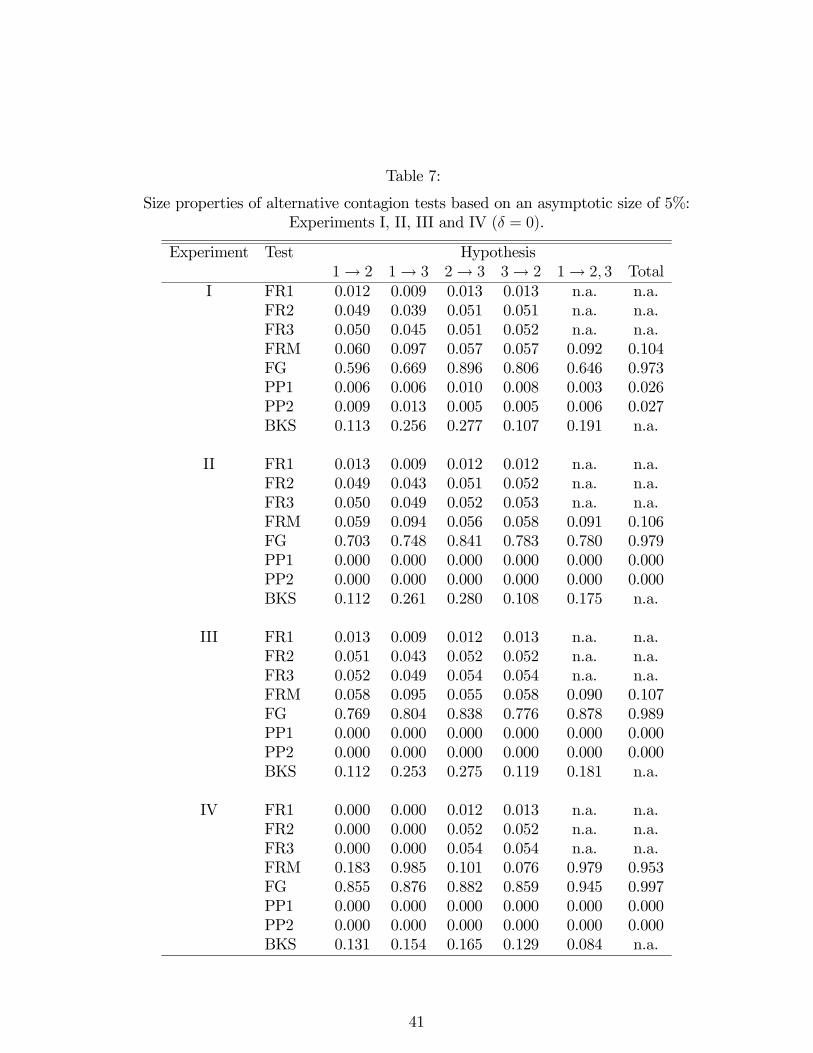
Table 7:

Size properties of alternative contagion tests based on an asymptotic size of 5%:Experiments I, II, III and IV (δ = 0).

Experiment Test Hypothesis1→ 2 1→ 3 2→ 3 3→ 2 1→ 2, 3 Total

I FR1 0.012 0.009 0.013 0.013 n.a. n.a.FR2 0.049 0.039 0.051 0.051 n.a. n.a.FR3 0.050 0.045 0.051 0.052 n.a. n.a.FRM 0.060 0.097 0.057 0.057 0.092 0.104FG 0.596 0.669 0.896 0.806 0.646 0.973PP1 0.006 0.006 0.010 0.008 0.003 0.026PP2 0.009 0.013 0.005 0.005 0.006 0.027BKS 0.113 0.256 0.277 0.107 0.191 n.a.

II FR1 0.013 0.009 0.012 0.012 n.a. n.a.FR2 0.049 0.043 0.051 0.052 n.a. n.a.FR3 0.050 0.049 0.052 0.053 n.a. n.a.FRM 0.059 0.094 0.056 0.058 0.091 0.106FG 0.703 0.748 0.841 0.783 0.780 0.979PP1 0.000 0.000 0.000 0.000 0.000 0.000PP2 0.000 0.000 0.000 0.000 0.000 0.000BKS 0.112 0.261 0.280 0.108 0.175 n.a.

III FR1 0.013 0.009 0.012 0.013 n.a. n.a.FR2 0.051 0.043 0.052 0.052 n.a. n.a.FR3 0.052 0.049 0.054 0.054 n.a. n.a.FRM 0.058 0.095 0.055 0.058 0.090 0.107FG 0.769 0.804 0.838 0.776 0.878 0.989PP1 0.000 0.000 0.000 0.000 0.000 0.000PP2 0.000 0.000 0.000 0.000 0.000 0.000BKS 0.112 0.253 0.275 0.119 0.181 n.a.

IV FR1 0.000 0.000 0.012 0.013 n.a. n.a.FR2 0.000 0.000 0.052 0.052 n.a. n.a.FR3 0.000 0.000 0.054 0.054 n.a. n.a.FRM 0.183 0.985 0.101 0.076 0.979 0.953FG 0.855 0.876 0.882 0.859 0.945 0.997PP1 0.000 0.000 0.000 0.000 0.000 0.000PP2 0.000 0.000 0.000 0.000 0.000 0.000BKS 0.131 0.154 0.165 0.129 0.084 n.a.

41

Table 8:

Size properties of alternative contagion tests based on an asymptotic size of 5%:Experiments V, VI, VII and VIII (δ = 0).

Experiment Test Hypothesis1→ 2 1→ 3 2→ 3 3→ 2 1→ 2, 3 Total

V FR1 0.000 0.003 0.227 0.002 n.a. n.a.FR2 0.010 0.080 0.939 0.178 n.a. n.a.FR3 0.003 0.025 0.548 0.024 n.a. n.a.FRM 0.065 0.381 0.066 0.065 0.336 0.320FG 0.527 0.604 0.913 0.548 0.649 0.983PP1 0.001 0.000 0.000 0.000 0.000 0.000PP2 0.001 0.004 0.001 0.000 0.001 0.002BKS 0.367 0.712 0.158 0.315 0.406 n.a.

VI FR1 0.000 0.003 0.221 0.002 n.a. n.a.FR2 0.011 0.082 0.921 0.175 n.a. n.a.FR3 0.003 0.026 0.537 0.024 n.a. n.a.FRM 0.060 0.099 0.055 0.057 0.096 0.109FG 0.537 0.609 0.911 0.553 0.659 0.983PP1 0.000 0.000 0.000 0.001 0.000 0.000PP2 0.001 0.003 0.001 0.000 0.001 0.002BKS 0.367 0.712 0.158 0.315 0.406 n.a.

VII FR1 0.001 0.000 0.015 0.014 n.a. n.a.FR2 0.002 0.000 0.051 0.052 n.a. n.a.FR3 0.002 0.000 0.051 0.053 n.a. n.a.FRM 0.084 0.463 0.064 0.055 0.425 0.370FG 0.756 0.774 0.235 0.230 0.861 0.920PP1 0.000 0.000 0.000 0.000 0.000 0.000PP2 0.000 0.000 0.000 0.000 0.000 0.000BKS 0.039 0.095 0.051 0.046 0.015 n.a.

VIII FR1 0.007 0.015 0.173 0.015 n.a. n.a.FR2 0.017 0.037 0.420 0.055 n.a. n.a.FR3 0.014 0.030 0.287 0.030 n.a. n.a.FRM 0.070 0.129 0.071 0.069 0.180 0.161FG 0.520 0.596 0.226 0.300 0.635 0.826PP1 0.000 0.000 0.000 0.000 0.000 0.000PP2 0.000 0.025 0.000 0.001 0.011 0.015BKS 0.179 0.934 0.086 0.108 0.378 n.a.

42

Table 9:

Experiment I: Power properties of alternative contagion tests, based on size adjustedcritical values of 5% (δ > 0).

Intensity Test Hypothesis1→ 2 1→ 3 2→ 3 3→ 2 1→ 2, 3 Total

δ = 1.0 FR1 0.115 0.288 0.080 0.060 n.a. n.a.FR2 0.119 0.295 0.091 0.067 n.a. n.a.FR3 0.115 0.288 0.080 0.060 n.a. n.a.FRM 0.070 0.187 0.049 0.054 0.181 0.123FG 0.035 0.033 0.041 0.046 0.032 0.038PP1 0.042 0.053 0.044 0.041 0.050 0.045PP2 0.051 0.066 0.042 0.040 0.059 0.057BKS 0.064 0.109 0.049 0.061 0.104 n.a.

δ = 2.0 FR1 0.209 0.378 0.184 0.087 n.a. n.a.FR2 0.220 0.394 0.249 0.125 n.a. n.a.FR3 0.209 0.378 0.184 0.087 n.a. n.a.FRM 0.061 0.439 0.104 0.089 0.384 0.411FG 0.034 0.028 0.040 0.047 0.026 0.040PP1 0.053 0.074 0.051 0.053 0.067 0.067PP2 0.066 0.103 0.048 0.042 0.095 0.085BKS 0.082 0.148 0.064 0.089 0.162 n.a.

δ = 5.0 FR1 0.434 0.328 0.404 0.075 n.a. n.a.FR2 0.481 0.189 0.810 0.280 n.a. n.a.FR3 0.434 0.328 0.404 0.075 n.a. n.a.FRM 0.102 0.481 0.983 0.720 0.416 0.997FG 0.051 0.040 0.041 0.065 0.042 0.050PP1 0.074 0.103 0.068 0.072 0.097 0.113PP2 0.103 0.152 0.062 0.056 0.150 0.147BKS 0.144 0.098 0.349 0.377 0.327 n.a.

δ = 10.0 FR1 0.573 0.463 0.218 0.046 n.a. n.a.FR2 0.629 0.076 0.923 0.394 n.a. n.a.FR3 0.573 0.463 0.218 0.046 n.a. n.a.FRM 0.168 0.197 1.000 0.938 0.179 1.000FG 0.078 0.068 0.042 0.060 0.063 0.056PP1 0.068 0.089 0.068 0.062 0.079 0.093PP2 0.119 0.137 0.056 0.049 0.135 0.121BKS 0.111 0.011 0.667 0.624 0.334 n.a.

43

Table 10:

Experiment II: Power properties of alternative contagion tests, based on size adjustedcritical values of 5% (δ > 0).

Intensity Test Hypothesis1→ 2 1→ 3 2→ 3 3→ 2 1→ 2, 3 Total

δ = 1.0 FR1 0.120 0.307 0.080 0.067 n.a. n.a.FR2 0.124 0.315 0.089 0.074 n.a. n.a.FR3 0.120 0.307 0.080 0.067 n.a. n.a.FRM 0.075 0.203 0.050 0.052 0.193 0.134FG 0.047 0.045 0.052 0.048 0.046 0.045PP1 0.048 0.042 0.047 0.047 0.045 0.044PP2 0.052 0.049 0.046 0.046 0.052 0.048BKS 0.063 0.101 0.045 0.066 0.105 n.a.

δ = 2.0 FR1 0.222 0.438 0.203 0.116 n.a. n.a.FR2 0.237 0.462 0.264 0.160 n.a. n.a.FR3 0.222 0.438 0.203 0.116 n.a. n.a.FRM 0.066 0.491 0.103 0.087 0.438 0.463FG 0.041 0.040 0.051 0.048 0.042 0.047PP1 0.052 0.046 0.044 0.052 0.045 0.044PP2 0.056 0.053 0.046 0.045 0.059 0.058BKS 0.080 0.146 0.059 0.089 0.162 n.a.

δ = 5.0 FR1 0.445 0.318 0.536 0.114 n.a. n.a.FR2 0.512 0.240 0.898 0.429 n.a. n.a.FR3 0.445 0.318 0.536 0.114 n.a. n.a.FRM 0.096 0.518 0.981 0.716 0.462 0.998FG 0.052 0.050 0.050 0.061 0.049 0.054PP1 0.062 0.049 0.045 0.066 0.055 0.060PP2 0.069 0.062 0.062 0.068 0.075 0.112BKS 0.155 0.122 0.329 0.365 0.354 n.a.

δ = 10.0 FR1 0.511 0.339 0.315 0.046 n.a. n.a.FR2 0.629 0.088 0.995 0.554 n.a. n.a.FR3 0.511 0.339 0.315 0.046 n.a. n.a.FRM 0.159 0.205 1.000 0.937 0.183 1.000FG 0.072 0.070 0.045 0.056 0.058 0.051PP1 0.063 0.045 0.047 0.069 0.054 0.071PP2 0.078 0.053 0.089 0.100 0.077 0.163BKS 0.108 0.017 0.639 0.611 0.350 n.a.

44

Table 11:

Experiment III: Power properties of alternative contagion tests, based on size adjustedcritical values of 5% (δ > 0).

Intensity Test Hypothesis1→ 2 1→ 3 2→ 3 3→ 2 1→ 2, 3 Total

δ = 1.0 FR1 0.115 0.306 0.079 0.067 n.a. n.a.FR2 0.119 0.313 0.088 0.074 n.a. n.a.FR3 0.115 0.306 0.079 0.067 n.a n.a.FRM 0.072 0.204 0.050 0.053 0.193 0.134FG 0.043 0.047 0.054 0.048 0.045 0.045PP1 0.048 0.046 0.051 0.046 0.044 0.045PP2 0.046 0.050 0.046 0.045 0.052 0.048BKS 0.070 0.110 0.046 0.059 0.102 n.a.

δ = 2.0 FR1 0.215 0.441 0.199 0.115 n.a. n.a.FR2 0.228 0.462 0.262 0.161 n.a. n.a.FR3 0.215 0.441 0.199 0.115 n.a. n.a.FRM 0.063 0.494 0.103 0.087 0.436 0.465FG 0.038 0.043 0.056 0.049 0.041 0.041PP1 0.051 0.046 0.046 0.050 0.051 0.047PP2 0.051 0.054 0.045 0.050 0.055 0.058BKS 0.087 0.152 0.062 0.087 0.165 n.a.

δ = 5.0 FR1 0.429 0.316 0.529 0.113 n.a. n.a.FR2 0.503 0.240 0.900 0.429 n.a. n.a.FR3 0.429 0.316 0.529 0.113 n.a. n.a.FRM 0.094 0.522 0.981 0.717 0.460 0.998FG 0.050 0.056 0.052 0.057 0.048 0.046PP1 0.062 0.051 0.054 0.068 0.059 0.072PP2 0.066 0.066 0.073 0.076 0.079 0.121BKS 0.151 0.140 0.332 0.353 0.349 n.a.

δ = 10.0 FR1 0.496 0.333 0.308 0.047 n.a. n.a.FR2 0.620 0.089 0.905 0.555 n.a. n.a.FR3 0.496 0.333 0.308 0.047 n.a. n.a.FRM 0.159 0.205 1.000 0.937 0.182 1.000FG 0.070 0.065 0.043 0.056 0.049 0.048PP1 0.065 0.053 0.058 0.073 0.065 0.091PP2 0.072 0.066 0.105 0.102 0.082 0.184BKS 0.113 0.023 0.649 0.612 0.348 n.a.

45

Table 12:

Experiment IV: Power properties of alternative contagion tests, based on size adjustedcritical values of 5% (δ > 0).

Intensity Test Hypothesis1→ 2 1→ 3 2→ 3 3→ 2 1→ 2, 3 Total

δ = 1.0 FR1 0.848 1.000 0.529 0.113 n.a. n.a.FR2 0.925 1.000 0.900 0.429 n.a. n.a.FR3 0.848 1.000 0.529 0.113 n.a. n.a.FRM 0.057 0.007 0.029 0.041 0.019 0.037FG 0.021 0.033 0.058 0.031 0.030 0.034PP1 0.042 0.039 0.033 0.044 0.039 0.039PP2 0.052 0.076 0.052 0.049 0.075 0.088BKS 0.169 0.741 0.084 0.102 0.464 n.a.

δ = 2.0 FR1 0.970 1.000 0.308 0.047 n.a. n.a.FR2 1.000 1.000 0.995 0.555 n.a. n.a.FR3 0.970 1.000 0.308 0.047 n.a. n.aFRM 0.017 0.425 0.535 0.360 0.451 1.000FG 0.023 0.028 0.051 0.027 0.026 0.031PP1 0.034 0.030 0.029 0.037 0.034 0.039PP2 0.053 0.061 0.054 0.055 0.069 0.122BKS 0.135 0.513 0.141 0.179 0.500 n.a.

δ = 5.0 FR1 0.984 1.000 0.055 0.028 n.a. n.a.FR2 1.000 1.000 0.993 0.525 n.a. n.a.FR3 0.984 1.000 0.055 0.028 n.a. n.a.FRM 0.027 0.022 1.000 0.822 0.027 1.000FG 0.051 0.046 0.039 0.031 0.029 0.031PP1 0.031 0.026 0.027 0.028 0.031 0.033PP2 0.039 0.042 0.052 0.050 0.050 0.117BKS 0.038 0.066 0.219 0.252 0.121 n.a.

δ = 10.0 FR1 0.985 1.000 0.031 0.026 n.a. n.a.FR2 1.000 1.000 0.930 0.396 n.a. n.a.FR3 0.985 1.000 0.031 0.026 n.a. n.a.FRM 0.024 0.000 1.000 0.698 0.000 1.000FG 0.084 0.080 0.034 0.034 0.032 0.032PP1 0.021 0.021 0.020 0.019 0.020 0.023PP2 0.028 0.029 0.036 0.034 0.036 0.078BKS 0.003 0.004 0.165 0.175 0.011 n.a.

46

Table 13:

Experiment V: Power properties of alternative contagion tests, based on size adjustedcritical values of 5% (δ > 0).

Intensity Test Hypothesis1→ 2 1→ 3 2→ 3 3→ 2 1→ 2, 3 Total

δ = 1.0 FR1 0.054 0.124 0.049 0.050 n.a. n.a.FR2 0.055 0.105 0.052 0.051 n.a. n.a.FR3 0.054 0.124 0.049 0.050 n.a. n.a.FRM 0.053 0.068 0.048 0.051 0.068 0.059FG 0.050 0.045 0.058 0.052 0.049 0.057PP1 0.044 0.046 0.047 0.044 0.043 0.045PP2 0.048 0.046 0.049 0.047 0.045 0.045BKS 0.046 0.053 0.043 0.044 0.049 n.a.

δ = 2.0 FR1 0.032 0.014 0.046 0.050 n.a. n.a.FR2 0.050 0.023 0.055 0.057 n.a. n.a.FR3 0.032 0.014 0.046 0.050 n.a. n.a.FRM 0.054 0.040 0.125 0.101 0.031 0.079FG 0.056 0.053 0.054 0.050 0.052 0.064PP1 0.055 0.054 0.060 0.056 0.054 0.059PP2 0.056 0.049 0.057 0.057 0.050 0.058BKS 0.055 0.044 0.077 0.074 0.061 n.a.

δ = 5.0 FR1 0.001 0.000 0.024 0.041 n.a. n.a.FR2 0.021 0.000 0.079 0.090 n.a. n.a.FR3 0.001 0.000 0.024 0.041 n.a. n.a.FRM 0.354 0.005 0.994 0.769 0.081 0.927FG 0.101 0.080 0.050 0.067 0.078 0.074PP1 0.088 0.083 0.095 0.087 0.088 0.114PP2 0.084 0.063 0.106 0.094 0.074 0.108BKS 0.049 0.009 0.464 0.416 0.083 n.a.

δ = 10.0 FR1 0.000 0.000 0.004 0.024 n.a. n.a.FR2 0.005 0.000 0.117 0.148 n.a. n.a.FR3 0.000 0.000 0.004 0.024 n.a. n.a.FRM 0.493 0.030 1.000 0.945 0.357 1.000FG 0.157 0.100 0.044 0.077 0.097 0.083PP1 0.097 0.089 0.110 0.100 0.097 0.146PP2 0.087 0.061 0.129 0.116 0.073 0.135BKS 0.016 0.000 0.768 0.584 0.025 n.a.

47

Table 14:

Experiment VI: Power properties of alternative contagion tests, based on size adjustedcritical values of 5% (δ > 0).

Intensity Test Hypothesis1→ 2 1→ 3 2→ 3 3→ 2 1→ 2, 3 Total

δ = 1.0 FR1 0.055 0.126 0.049 0.050 n.a. n.a.FR2 0.055 0.102 0.052 0.052 n.a. n.a.FR3 0.055 0.126 0.049 0.050 n.a. n.a.FRM 0.075 0.195 0.051 0.053 0.189 0.131FG 0.046 0.047 0.051 0.045 0.052 0.051PP1 0.044 0.044 0.046 0.047 0.045 0.048PP2 0.045 0.045 0.048 0.047 0.042 0.045BKS 0.046 0.053 0.043 0.044 0.049 n.a.

δ = 2.0 FR1 0.034 0.014 0.046 0.049 n.a. n.a.FR2 0.051 0.024 0.057 0.058 n.a. n.a.FR3 0.034 0.014 0.046 0.049 n.a. n.a.FRM 0.066 0.491 0.103 0.087 0.441 0.466FG 0.055 0.054 0.054 0.048 0.054 0.051PP1 0.055 0.054 0.056 0.060 0.058 0.059PP2 0.057 0.053 0.057 0.058 0.054 0.057BKS 0.055 0.044 0.077 0.074 0.061 n.a.

δ = 5.0 FR1 0.001 0.000 0.025 0.041 n.a. n.a.FR2 0.021 0.000 0.080 0.092 n.a. n.a.FR3 0.001 0.000 0.025 0.041 n.a. n.a.FRM 0.093 0.529 0.979 0.713 0.478 0.998FG 0.093 0.088 0.045 0.063 0.089 0.065PP1 0.093 0.081 0.094 0.094 0.095 0.122PP2 0.084 0.069 0.104 0.093 0.074 0.112BKS 0.049 0.009 0.464 0.416 0.083 n.a.

δ = 10.0 FR1 0.000 0.000 0.004 0.024 n.a. n.a.FR2 0.005 0.000 0.121 0.150 n.a. n.a.FR3 0.000 0.000 0.004 0.024 n.a. n.a.FRM 0.156 0.218 1.000 0.937 0.201 1.000FG 0.148 0.114 0.040 0.072 0.105 0.072PP1 0.099 0.092 0.108 0.107 0.100 0.152PP2 0.089 0.064 0.125 0.113 0.075 0.139BKS 0.016 0.000 0.768 0.584 0.025 n.a.

48

Table 15:

Experiment VII: Power properties of alternative contagion tests, based on size adjustedcritical values of 5% (δ > 0).

Intensity Test Hypothesis1→ 2 1→ 3 2→ 3 3→ 2 1→ 2, 3 Total

δ = 1.0 FR1 0.447 0.904 0.400 0.129 n.a. n.a.FR2 0.487 0.934 0.408 0.129 n.a. n.a.FR3 0.460 0.904 0.287 0.069 n.a. n.a.FRM 0.048 0.006 0.053 0.065 0.025 0.022FG 0.021 0.031 0.077 0.089 0.033 0.045PP1 0.044 0.040 0.046 0.062 0.045 0.056PP2 0.072 0.151 0.061 0.087 0.149 0.190BKS 0.284 0.979 0.117 0.123 0.473 n.a.

δ = 2.0 FR1 0.687 0.957 0.261 0.079 n.a. n.a.FR2 0.756 0.976 0.374 0.096 n.a. n.a.FR3 0.693 0.957 0.170 0.041 n.a. n.aFRM 0.059 0.057 0.093 0.093 0.129 0.325FG 0.010 0.016 0.119 0.175 0.014 0.059PP1 0.042 0.035 0.041 0.060 0.041 0.055PP2 0.067 0.132 0.095 0.123 0.139 0.321BKS 0.377 0.848 0.566 0.587 0.808 n.a.

δ = 5.0 FR1 0.770 0.955 0.088 0.059 n.a. n.a.FR2 0.838 0.977 0.181 0.059 n.a. n.a.FR3 0.774 0.955 0.049 0.033 n.a. n.a.FRM 0.079 0.008 0.217 0.141 0.111 0.552FG 0.014 0.016 0.134 0.211 0.009 0.056PP1 0.037 0.036 0.043 0.048 0.042 0.054PP2 0.069 0.086 0.174 0.170 0.102 0.431BKS 0.351 0.276 0.701 0.704 0.976 n.a.

δ = 10.0 FR1 0.773 0.957 0.062 0.055 n.a. n.a.FR2 0.839 0.978 0.097 0.042 n.a. n.a.FR3 0.776 0.957 0.035 0.031 n.a. n.a.FRM 0.083 0.003 0.191 0.151 0.099 0.595FG 0.031 0.031 0.122 0.172 0.011 0.051PP1 0.029 0.031 0.035 0.037 0.033 0.040PP2 0.056 0.063 0.156 0.156 0.082 0.364BKS 0.156 0.075 0.486 0.487 0.992 n.a.

49

Table 16:

Experiment VIII: Power properties of alternative contagion tests, based on size adjustedcritical values of 5% (δ > 0).

Intensity Test Hypothesis1→ 2 1→ 3 2→ 3 3→ 2 1→ 2, 3 Total

δ = 1.0 FR1 0.052 0.083 0.047 0.050 n.a. n.a.FR2 0.052 0.089 0.048 0.050 n.a. n.a.FR3 0.053 0.091 0.047 0.049 n.a. n.a.FRM 0.048 0.047 0.044 0.052 0.047 0.047FG 0.051 0.050 0.050 0.047 0.051 0.046PP1 0.046 0.048 0.044 0.047 0.044 0.044PP2 0.047 0.047 0.052 0.050 0.048 0.048BKS 0.052 0.045 0.043 0.043 0.051 n.a.

δ = 2.0 FR1 0.045 0.025 0.043 0.051 n.a. n.a.FR2 0.049 0.026 0.046 0.050 n.a. n.a.FR3 0.045 0.023 0.044 0.049 n.a. n.a.FRM 0.069 0.058 0.085 0.064 0.068 0.081FG 0.054 0.052 0.054 0.058 0.053 0.052PP1 0.053 0.057 0.056 0.056 0.055 0.055PP2 0.051 0.053 0.057 0.056 0.053 0.057BKS 0.051 0.039 0.083 0.085 0.078 n.a.

δ = 5.0 FR1 0.018 0.001 0.028 0.050 n.a. n.a.FR2 0.022 0.001 0.045 0.050 n.a. n.a.FR3 0.016 0.001 0.029 0.048 n.a. n.a.FRM 0.170 0.302 0.624 0.208 0.377 0.556FG 0.076 0.064 0.065 0.103 0.064 0.071PP1 0.087 0.084 0.074 0.082 0.095 0.104PP2 0.060 0.039 0.106 0.102 0.043 0.083BKS 0.037 0.001 0.546 0.571 0.175 n.a.

δ = 10.0 FR1 0.007 0.001 0.008 0.040 n.a. n.a.FR2 0.013 0.001 0.036 0.046 n.a. n.a.FR3 0.006 0.000 0.007 0.036 n.a. n.a.FRM 0.109 0.313 0.786 0.165 0.410 0.795FG 0.113 0.074 0.080 0.143 0.067 0.090PP1 0.095 0.094 0.095 0.098 0.106 0.141PP2 0.064 0.021 0.187 0.153 0.025 0.125BKS 0.052 0.000 0.944 0.944 0.121 n.a.

50

where a 0 denotes the first derivative. Using the expressions for g (x) and h (x)

g01 (v) =1√v2v3

g02 (v) = −12v1v

−3/22 v

−1/23

g03 (v) = −12v1v

−1/22 v

−3/23

g04 (v) = g05 (v) = g06 (v) = 0

h01 (v) = h02 (v) = h03 (v) = 0

h04 (v) =1√v5v6

h05 (v) = −12v4v

−3/25 v

−1/26

h06 (v) = −12v4v

−1/25 v

−3/26 .

Substituting into the expression for the covariance in (56) and evaluating at the population

value θ, gives

Cov (ry, r) = (θ2θ3)−1/2 (θ5θ6)

−1/2Cov (v1, v4)

−12θ−1/22 θ

−1/23 θ4θ

−3/25 θ

−1/26 Cov (v1, v5)

−12θ−1/22 θ

−1/23 θ4θ

−3/25 θ

−1/26 Cov (v1, v6)

−12θ1θ

−3/22 θ

−1/23 θ

−1/25 θ

−1/26 Cov (v2, v4)

+1

4θ1θ

−3/22 θ

−1/23 θ4θ

−3/25 θ

−1/26 Cov (v2, v5)

+1

4θ1θ

−3/22 θ

−1/23 θ4θ

−1/25 θ

−3/26 Cov (v2, v5)

−12θ1θ

−1/22 θ

−3/23 θ

−1/25 θ

−1/26 Cov (v3, v4)

+1

4θ1θ

−1/22 θ

−3/23 θ4θ

−3/25 θ

−1/26 Cov (v3, v5)

+1

4θ21θ

−1/22 θ

−3/23 θ4θ

−1/25 θ

−3/26 Cov (v3, v6) .

Using the result that under the the null, the distribution is standardized bivariate normal,

then

θ1 = θ4 = ρ, θ2 = θ3 = θ5 = θ6 = 1,

51

and the expression for Cov (ry, r) simplifies to

Cov (ry, r) = Cov (v1, v4)− ρ

2(Cov (v1, v5) + Cov (v1, v6) + Cov (v2, v4) + Cov (v3, v4))

+ρ2

4(Cov (v2, v5) + Cov (v2, v6) + Cov (v3, v5) + Cov (v3, v6)) . (57)

This expression simplifies even further for the case of contemporaneous independence (ρ = 0)

Cov (ry, r) = Cov (v1, v4) . (58)

Now consider the sample covariances

v1 = m11 =1

Ty

TyXt=1

(y1,t − y1) (y2,t − y2)

v4 = n11 =1

T

TXt=1

(z1,t − z1) (z2,t − z2) . (59)

It is helpful to rewrite the covariance for the total sample period as

n11 =1

T

TXt=1

(z1,t − z1) (z2,t − z2)

=1

T

ÃTxXt=1

(x1,t − x1) (x2,t − x2) +TX

t=Tx+1

(y1,t − y1) (y2,t − y2)

!

=1

T

ÃTxXt=1

(x1,t − x1) (x2,t − x2)

!+

TyTm11,

so

Cov (v1, v4) = Cov

Ãn11,

1

T

ÃTxXt=1

(x1,t − x1) (x2,t − x2)

!+

TyTm11

!. (60)

Because of independence, this expression immediately reduces to

Cov (v1, v4) = Cov

µn11,

TyTm11

¶=

TyTV ar (m11) (61)

An expression for V ar (m11) is obtained using the property of the standard errors of bivariate

moments (Kendall and Stuart, (1969, Vol.1, p.232))

V ar (m11) =1

Ty

¡μ2,2 − μ21,1 + μ2,0μ

20,1 + μ0,2μ

21,0 + 2μ1,1μ0,1μ1,0 − 2μ2,1μ0,1 − 2μ1,2μ1,0

¢,

(62)

52

which reduces to

V ar (m11) =1

Ty

¡μ2,2 − μ21,1

¢=

1

Ty

¡1 + 2ρ2 − ρ2

¢(63)

as μ0,1 = μ1,0 = 0 because the random variables have zero mean, and for the standardized

bivariate normal distribution μ2,2 = 1 + 2ρ2, μ21,1 = ρ2. For the case of contemporaneous

independence (ρ = 0) then V ar (m11) = T−1y and from (61)

Cov (ry, r) =TyT

1

Ty=1

T. (64)

Finally, using the result that the distribution is bivariate normal and contemporaneously

independent, V ar (ry) = T−1y and V ar (r) = T−1, gives the key result

V ar (ry − r) = V ar (ry) + V ar (r)− 2Cov (ry, r)=

1

Ty+1

T− 2 1

T

=1

Ty− 1

T. (65)

53

References

[1] Bae, K.H, Karolyi, G.A. and Stulz, R.M. (2003), “A New Approach to Measuring

Financial Contagion”, Review of Financial Studies, 16(3), 717-763.

[2] Baig, T. and Goldfajn, I. (1999), “Financial Market Contagion in the Asian Crisis”,

IMF Staff Papers, 46(2), 167-195.

[3] Banerjee, A. and Urga, G. (2005),“Modelling Structural Breaks, Long Memory and

Stock Market Volatility: An Overview”, Journal of Econometrics, 129, 1-34.

[4] Baur, D. and Schulze, N. (2002), “Coexceedances in Financial Markets - A Quantile

Regression Analysis of Contagion”, University of Tuebingen Discussion Paper 253.

[5] Bekaert, G., Harvey, C.R. and Ng, A. (2005), “Market Integration and Contagion”,

Journal of Business, 78(1), part 2, forthcoming.

[6] Billio, M. and Pelizzon, L. (2003), “Contagion and Interdependence in Stock Markets:

Have They Been Misdiagnosed?”, Journal of Economics and Business, 55 405-426.

[7] Ciccarelli, M. and Rebucci, A. (2004), “Measuring Contagion and Interdependence with

a Bayesian Time-Varying Coefficient Model: The Chilean FX Market During the Ar-

gentine Crisis”, mimeo.

[8] Corsetti, G., Pericoli, M. and Sbracia, M. (2002), “Some Contagion, Some Interdepen-

dence’: More Pitfalls in Testing for Contagion”, mimeo University of Rome III.

[9] Dasgupta, A. (2000), “Regionality Revisited: An Examination of the Direction of Spread

of Currency Crises”, mimeo, LSE.

[10] Dornbusch, R., Park, Y.C. and Claessens, S. (2000), “Contagion: Understanding How

It Spreads”, The World Bank Research Observer, 15(2), 177-97.

[11] Dungey, M., Fry, R., González-Hermisillo, B. and Martin, V.L. (2002), “The Trans-

mission of Contagion in Developed and Developing International Bond Markets”, in

Committee on the Global Financial System (ed), Risk Measurement and Systemic Risk,

Proceedings of the Third Joint Central Bank Research Conference, 61-74 .

54

[12] Dungey, M., Fry, R., Gonzalez-Hermosillo, B. and Martin, V.L. (2005a), “A Comparison

of Alternative Tests of Contagion with Applications”, in M. Dungey and D. Tambakis

(eds) Identifying International Financial Contagion: Progress and Challenges, Oxford

University Press, 60-85.

[13] Dungey, M., Fry, R., González-Hermosillo, B. and Martin, V.L. (2005b), “Empirical

Modelling of Contagion: A Review of Methodologies”, Quantitative Finance, 5(1), 9-

24.

[14] Dungey, M. and Martin, V.L. (2004), “A Multifactor Model of Exchange Rates with

Unanticipated Shocks: Measuring Contagion in the East Asian Currency Crisis”, Jour-

nal of Emerging Markets Finance, 3, 305-330.

[15] Dungey, M., Fry, R., González-Hermosillo, B. and Martin, V.L. (2005c) “Contagion in

International BondMarkets During the Russian and LTCM crises”, Journal of Financial

Stability, forthcoming.

[16] Dungey, M., Martin, V.L. and Pagan, A.R. (2000), “A Multivariate Latent Factor

Decomposition of International Bond Yield Spreads”, Journal of Applied Econometrics,

15, 697-715.

[17] Eichengreen, B., Rose, A.K. and Wyplosz, C. (1995), “Exchange Market Mayhem: The

Antecedents and Aftermath of Speculative Attacks”, Economic Policy, 21, 249-312.

[18] Eichengreen, B., Rose, A.K. and Wyplosz, C. (1996), “Contagious Currency Crises”,

NBER Working Paper, 5681.

[19] Engle, R.F., (2004), “Risk and Volatility: Econometric Models and Financial Practice,

American Economic Review, 94, 405-420.

[20] Favero, C.A. and Giavazzi, F. (2002), “Is the International Propagation of Financial

Shocks Non-linear? Evidence From the ERM”, Journal of International Economics, 57

(1), 231-46.

[21] Forbes, K. and Rigobon, R. (2002), “No Contagion, Only Interdependence: Measuring

Stock Market Co-movements”, Journal of Finance, 57 (5), 2223-61.

55

[22] Glick, R. and Rose, A.K. (1999), “Contagion and Trade: Why are Currency Crises

Regional?”, Journal of International Money and Finance, 18(4), 603-17.

[23] Hahn, J. and Hausman, J. (2002), “A New Specification Test for the Validity of Instru-

mental Variables”, Econometrica, 70, 163-189.

[24] Jeanne, O., and Masson, P. (2000), “Currency Crises, Sunspots and Markov-Switching

Regimes”, Journal of International Economics, 50(2), 327-350.

[25] Kaminsky, G.L. and Reinhart, C.M. (2000), “On Crises, Contagion and Confusion”,

Journal of International Economics, 51(1), 145-168.

[26] Kaminsky, G.L. and Reinhart, C.M. (2001), “Financial Markets in Times of Stress”,

NBER Working Paper, 8569.

[27] Kendall, M. and Stuart, A. (1969), The Advanced Theory of Statistics, Vol.1, Charles

Griffin and Co., London.

[28] Kendall, M. and Stuart, A. (1973), The Advanced Theory of Statistics, Vol.2, Charles

Griffin and Co., London.

[29] Loretan, M. and English, W. (2000), “Evaluating "Correlation Breakdowns" During

Periods of Market Volatility”, Board of Governors of the Federal Reserve System, In-

ternational Finance Discussion Paper No. 658.

[30] Lowell, J., Neu, C.R. and Tong, D. (1998), “Financial Crises and Contagion in Emerging

Market Countries”, Monograph, RAND.

[31] Mody, A, and Taylor, M.P. (2003), “Common Vulnerabilities”, CEPR Discussion Paper

3759.

[32] Nelson, C.R. and Startz, R. (1990a), “Some Further Results on the Exact Small Sample

Properties of the Instrumental Variables Estimator”, Econometrica, 58, 967-976.

[33] Nelson, C.R. and Startz, R. (1990b), “The Distribution of the Instrumental Variables

Estimator and Its t-Ratio When the Instrument is a Poor One”, Journal of Business,

63, S125-S140.

56

[34] Pesaran, H. and Pick, A. (2003), “Econometric Issues in the Analysis of Contagion”,

CESifo Working Paper 1176.

[35] Pericoli, M. and Sbracia, M. (2003), “A Primer on Financial Contagion”, Journal of

Economic Surveys, 17(4), 571-608.

[36] Pritsker, M. (2002), “Large Investors and Liquidity: A Review of the Literature”, in

Committee on the Global Financial System (ed), Risk Measurement and Systemic Risk,

Proceedings of the Third Joint Central Bank Research Conference.

[37] Rigobon, R. (2003), “On the Measurement of the International Propogation of Shocks:

Is the Transmission Stable?”, Journal of International Economics, 61, 261-283.

[38] Stock, J.H., Wright, J.H. and Yogo, M. (2002), “A Survey of Weak Instruments and

Weak Identification in Generalized Method of Moments”, Journal of Business and Eco-

nomic Statistics, 20(4), 518-529.

[39] Walti, S. (2003), “Testing for Contagion in International Financial Markets: Which

Way to Go?”, The Graduate Institute of International Studies, Geneva, HEI Working

Paper No: 04/2003.

57