Sampling-based stochastic analysis of the PKN model for

hydraulic fracturing

Abstract

The hydraulic fracturing process is surrounded by uncertainty, as available data is typicallyscant. In this work we present a sampling-based stochastic analysis of the hydraulic fracturingprocess by considering various system parameters to be random. Our analysis is based on thePerkins-Kern-Nordgren (PKN) model for hydraulic fracturing. This baseline model enablescomputation of high fidelity solutions, which avoids pollution of our stochastic results by in-accuracies in the deterministic solution procedure. In order to obtain the desired degree ofaccuracy of the computed solution we supplement the employed time-dependent moving-meshfinite element method with two enhancements: i) global conservation of volume is enforcedthrough a Lagrange-multiplier; ii) the weakly-singular behavior of the solution at the frac-ture tip is resolved by supplementing the solution space with a tip enrichment function. Thistip enrichment function enables the computation of the tip-speed directly from its associatedsolution coefficient. An incremental-iterative solution procedure based on a backward-Eulertime-integrator with sub-iterations is employed to solve the PKN model. Direct Monte Carlosampling is performed based on random variable and random field input parameters. Thepresented stochastic results quantify the dependence of the fracture evolution process – in par-ticular the fracture length and fracture opening – on variations in the elastic properties andleak-off coefficient of the formation, and the height of the fracture.

1

1 Introduction

Hydraulic fracturing processes – i.e. the fracturing of rock formations by a pressurized liquid toimprove connectivity of reservoirs and geothermal formations – are surrounded by uncertainty,as available formation data is limited. Further improvement of models and simulation tools tounderstand this process is instrumental to increasing operational effectivity and to reliably quantifythe risks and uncertainties that are involved.

Hydraulic fracturing models involve the coupling of three sub-models: i) a solid mechanicsmodel which describes the deformation of the rock formation induced by the fluid load; ii) afluid flow model to describe the fracturing-fluid in the crack, as well as its leak-off into the rockformation; iii) a fracture mechanics model including a fracture propagation criterion. Intrinsiccharacteristics of such models are the (strong) non-linearities related to the coupling betweenthe solid and fluid, the singularities in the physical fields near the fracture front, the moving(fracture) domain boundaries, the degeneration of the governing equations near the tip region,and pronounced multiscale effects with the length scales varying from millimeters for the fractureopening near the tip to kilometers for the length of the fracture.

Various practical model simplifications – most commonly restricting the model to a singletwo-dimensional planar fracture – have been proposed, the most prominent of which are: i) ThePerkins-Kern-Nordgren (PKN) model [1, 2] for a fracture of fixed height and elliptical cross sec-tion (leveraging the Sneddon solution for the elasticity problem [3]) which propagates horizontallyin one direction; ii) The radial model for a horizontal Penny-shaped crack that evolves evenlyin all directions in accordance with Sneddon’s solution [4]; iii) The Khristianovic-Geertsma-DeKlerk (KGD) model [5, 6, 7] for a vertical fracture of fixed height that propagates horizontally inone direction. Various pseudo-three-dimensional (P3D) models [8] and planar-three-dimensional(PL3D) models [9, 10] have been proposed over the years to enable consideration of more complexfracture patterns and fractures in multi-layer formations. These P3D models typically extend theabove-mentioned two-dimensional models by considering a variation of fracture height in combi-nation with fracture length and width. Although these classical models are generally based onrestrictive and often ad-hoc assumptions, they are still widely used in the industry [11].

Despite the simplifications in the above-mentioned models, analytical solutions can only beobtained in limiting cases (see e.g. [5, 6, 2]). General solution strategies for these models relyon the use of computational techniques. Versatile and reliable simulators for hydraulic fracturingprocesses are indispensable in gaining further understanding of the process, in particular becausedirect observation possibilities (typically several kilometers below the earth surface) are limited.The most prominent computational techniques used for hydraulic fracturing are Finite VolumeMethods [12], Finite Element Methods [13, 14, 15], Boundary Integral Methods [16] and DiscreteElement Methods [17]. Recent advancements in numerical methods for hydraulic fracturing thatare particularly noteworthy are the eXtended Finite Element Techniques (X-FEM) [18] and phase-field methods [19].

Although the importance of considering realistic geological situations is acknowledged [20], hy-draulic fracture evolution in formations with uncertain heterogeneous rock properties (e.g. elasticmoduli, compression/tensile strength, porosity, permeability) have not been studied in detail. Thepossibility of considering stochastic heterogeneities has been explored in [21], where the initiationand evolution of fracture has been studied using Monte Carlo sampling. The main challenge in suchstudies relates to the computational feasibility, in the sense that the computational effort of thedeterministic simulations (whose error must be controlled in relation to the stochastic variations)makes them impractical in the context of sampling-based stochastic techniques.

In this work we present a detailed probabilistic analysis of the hydraulic fracturing processbased on Monte Carlo simulations. The computational tractability of the stochastic frameworkconsidered herein motivates the use of the two-dimensional PKN model. We represent the (epis-temic) uncertain parameters of the PKN model as random variables and/or random fields, andinvestigate the influence of these uncertain input parameters on the fracture geometry (in particu-lar the fracture length and opening at the well bore). As part of the stochastic analysis we presenta sensitivity analysis of the deterministic model. It is worth mentioning that similar analyses can

2

i(t)

x

y

z

L(t)

H

w(x, t)

Figure 1: Schematic diagram of PKN fracture

be found in the literature for the deterministic setting [22, 23]. The primary focus of this work isthe direct analysis of the propagation of heterogeneous uncertainties in the hydraulic fracturingprocess. As part of this study we present a detailed derivation of the PKN model in the context ofrandom (spatially correlated) heterogeneous data. Control over accuracy is of paramount impor-tance, as stochastic uncertainty quantification should not be polluted by numerical inaccuracies.In this regard we propose to use two features in the numerical method for the PKN model tocontrol its accuracy: i) a Lagrange multiplier method to enforce the conservation of volume; ii)a special enrichment function for the finite element discretization of the PKN model to overcometip singularity issues.

In Section 2 the governing equations are discussed, with a special focus on the incorporationof rock heterogeneities in the PKN model. In Section 3, the weak formulation and finite elementdiscretization of the model are presented including various algorithmic details. The stochastic set-ting and Monte Carlo method are introduced in Section 4, where the random field discretizationof the heterogeneous properties using the Karhunen-Loeve expansion is also discussed. Numericalsimulations are presented in Section 5 to study the influence of input uncertainties in hydraulicfracturing. Finally, conclusions are presented in Section 6.

2 The PKN model for hydraulic fracturing

In this section we review the PKN model for hydraulic fracturing in the context of stochasticanalysis with heterogeneous random fields. The PKN model – which was originally formulatedby Perkins and Kern [1] and later amended with a leak-off model by Nordgren [2] and a propa-gation condition by Kemp [24] – is a practical candidate for studying the probabilistic behaviorof hydraulic fracturing by virtue of its computational tractability. Although highly simplified, thePKN model is based on fundamental physical principles and is capable of generating practicallymeaningful results [25].

3

z

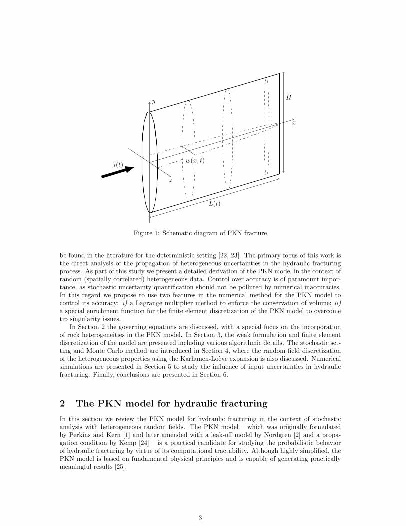
Figure 2: PKN fracture in xz plane where height is constant y direction, the length and width isvarying

2.1 Problem definition

The key assumption of the PKN model is that it considers a planar fracture with a constant heightH; see Figure 1. Displacements and displacement gradients in the surrounding solid are assumedto remain small, and the material is assumed to be linear elastic and isotropic. The fracturesurface resides in the xy-plane, while the fracture opens in the z-direction. The fracture aperturein the fracture plane is denoted by w(x, y, t), and the aperture at the y = 0 center line by w(x, t).The fracture connects to the well at x = 0 and its evolving front is situated at x = L(t).

A Newtonian fluid is injected into the fracture at the well with a controlled flow rate i(t), andthe flow inside the permeable crack is assumed to be laminar. The fracture process is assumed tobe in the viscosity-based regime, where toughness effects can be neglected (propagation is governedby friction and leak-off effects). At the front of the fracture fluid lag is assumed to be zero, i.e.,the fracture front coincides with the fluid front. Moreover, spurt losses due to the creation of newfracture surface are ignored.

2.2 Governing equations

In this section the governing equations of the sub-models are reviewed. In the presented derivationswe focus on those aspects of the sub-models that need careful consideration in the context of thestochastic analysis discussed in the remainder of this work.

2.2.1 Fluid flow model

The PKN model is based on the conservation of mass of the fluid, which establishes a link betweenthe injected volume, the created fracture volume and the leak-off volume. The differential materialbalance for the fracturing fluid is given by

∂q

∂x+∂A

∂t= −scl x ∈ (0, L(t)), (1)

where q(x, t) is the volume rate of flow through the cross-sectional area A(x, t) and scl(x, t) isthe rate of fluid volume loss per unit length of the fracture. At the well the flow rate is equal toq(0, t) = i(t).

The flow rate inside the fracture is related to the pressure gradient by assuming Poiseuille flow[26]. For such a flow the advective terms are assumed to remain small, so that the incompressibleNavier-Stokes equations reduce to the Stokes equations. The PKN model moreover assumes ahorizontal slot flow [27] with a parabolic fluid velocity profile

v = − 1

2µf

∂p

∂x

(w2

4− z2

)(2)

where w(x, y, t) is the opening of the fracture and µf is the fluid viscosity. As will be discussedin more detail in the context of the solid model, the assumptions of the PKN model render the

4

cross-section to be ellipsoidal. The fracture aperture is then given by

w = w√

1− 4y2/H2, (3)

where w is the maximum aperture at y = 0. The cross-sectional area is then equal to A(x, t) =π4Hw(x, t) and the fluid flow follows by integration of (2) as

q =

H/2∫−H/2

w/2∫−w/2

v dydz = − 1

12µf

∂p

∂x

H/2∫−H/2

w3 dy = −πHw3

64µf

∂p

∂x. (4)

The leak-off volume rate per unit length of fracture in equation (1) follows the phenomenologicallaw proposed by Carter [28]:

scl =2Hcl√t− τ(x)

(5)

In this expression cl is the leak-off coefficient and τ is the arrival time of the fracture tip at locationL, i.e. τ = L−1(x). The main assumptions behind this model are that: i) the fracturing fluiddeposits a thin layer of relatively low permeability known as the filter cake on the inner faces ofthe fracture, with the deposition rate being proportional to the leak-off rate, and ii) the viscosityof the filtrate is high enough to fully displace the fluid already present in the rock pores.

Substitution of equations (4) and (5) in the material balance (1) then yields the fluid flow massbalance:

πH

64µf

∂

∂x

(w3 ∂p

∂x

)=

2Hcl√t− τ(x)

+πH

4

∂w

∂tx ∈ (0, L(t)) (6)

2.2.2 Solid deformation model

To derive the relation between the fluid pressure and the solid deformation as used in the PKNmodel we consider the infinite domain Ω = R3

+ with evolving fracture surface Γc(t) = x ∈ Ω |0 ≤ x ≤ L(t),−H/2 ≤ y ≤ y, z = 0. Assuming inertia and gravity effects to be negligible, thesolid deformation, u = (u, v, w), follows from the momentum balance

∇ · σ = 0 in Ω (7)

where σ is the Cauchy stress. Along the fracture surface the solid is loaded by the fluid pressure,i.e. σn = −pn on Γ±c where n is the normal vector pointing into the fluid domain. The Cauchystress follows Hooke’s law for isotropic materials

σ = 2µsε+ λstr(ε)I, (8)

where the Lame parameters µs(x) and λs(x) are heterogeneous fields directly related to theYoung’s modulus, E(x), and Poisson’s ratio, ν(x). In Section 4 we will model the elastic propertiesby means of random fields, which are parametrized by a mean value, a standard deviations, and anauto-correlation length, c. This auto-correlation length is a measure of the correlation between anytwo material points in a random field, where a large correlation length implies that the frequencyof the heterogeneous field is low.

To derive the elasticity relation for the PKN model it is assumed that deformations are pla-nar, in the sense that the solid does not deform in the direction of the fracture propagation (thex-direction), and a plane strain condition in that direction applies. The auto-correlation lengthmust be sufficiently large not to violate these assumptions. Moreover, we herein neglect hetero-geneous variations perpendicular to the fracture propagation direction. Under these assumptions,combination of the momentum balance (7) and constitutive relation (8) yields

2µs(x)∂2v

∂y2+ λs(x)

(∂2v

∂y2+

∂2w

∂y∂z

)+ µs(x)

(∂2v

∂z2+

∂2w

∂y∂z

)= 0

µs(x)

(∂2v

∂y∂z+∂2w

∂y2

)+ 2µs(x)

∂2w

∂z2+ λs(x)

(∂2v

∂y∂z+∂2w

∂z2

)= 0

(9)

5

at an arbitrary plane perpendicular to the x-direction. Supplemented with the boundary conditionsσzz(x) = −p(x) and σyz(x) = 0 on the fracture boundary and vanishing far field conditions, thisproblem can be solved analytically. The fracture opening in the case of a constant pressure in theyz-plane is given by (see e.g. Lowengrub [29] and Sneddon [3] for details)

w(x, y) = 4p(x)

∫ H/2

y

y(1− ν(x)2)

E(x)√y2 − y2

dy =2Hp(x)

E′(x)

√1− 4y2/H2 0 ≤ y ≤ H/2, (10)

where E′(x) = E(x)/(1 − ν(x)2) is the plane strain modulus which is heterogeneous only in thex-direction. The elliptical profile (3) is a direct result of the setting of the elasticity problemconsidered here, with the maximum aperture equal to

w(x) =2Hp(x)

E′(x). (11)

An essential property of this solution is that along the crack path the fracture aperture is linearlyrelated to the pressure. The local nature of this relation is a direct consequence of the assumedplanar deformation. Note that the stress field and displacement field can be derived in the formof special integral representations [30].

2.2.3 Fracture propagation model

In the PKN model it is assumed that once the fracture has exceeded a certain distance, theenergy dissipation associated with the fracture of the rock material is small compared to energydissipation associated with the viscous flow of the fracturing fluid. This effectively neglects thefracture toughness, and fracture propagation is purely driven by the fluid velocity. Herein weadopt the standard assumption of zero fluid lag [2] – i.e., the velocity of the fluid at the fluid frontand the tip propagation speed are equal – so that tip propagation follows the Stefan condition

v(L(t), t) = limx→L(t)

q(x, t)

A(x, t)= L(t). (12)

Substitution of the flow rate (4) and surface area then yields:

L(t) = − 1

16µflim

x→L(t)w2 ∂p

∂x(13)

2.3 The coupled initial boundary value problem

The hydraulic fracture problem is characterized by a strong coupling of the sub-models discussedabove. The solid deformation is coupled to the fluid through the pressure loading along thefracture surface, while the fluid flow depends on the fracture opening though the Poiseuille flowprofile. The fracture propagation condition is coupled directly to the fluid flow through the Stefancondition (12), and in turn influences the fluid flow by virtue of the fact that fracture propagationextends the fluid flow domain. The pointwise relation between pressure and the fracture openingin equation (11) allows the formulation of a single-field problem. Herein we consider the initialboundary value problem for the fracture opening on the time interval (0, T ) 3 t with evolving

6

domain (0, L(t)) 3 x:

π

128µf

∂

∂x

(w3 ∂ (E′w)

∂x

)=

2Hcl√t− τ

+πH

4

∂w

∂t∀x ∈ (0, L(t)), ∀t ∈ ×(0, T )

− π

128µf

(w3 ∂ (E′w)

∂x

)∣∣∣∣x=0

= i(t) ∀t ∈ (0, T )

w(L(t), t) = 0 ∀t ∈ (0, T )

w(x, 0) = 0 ∀x ∈ (0, L0)

L(t) = − 1

96µfH

∂(E′w3

)∂x

∣∣∣∣∣x=L(t)

∀t ∈ (0, T )

L(0) = L0

(14a)

(14b)

(14c)

(14d)

(14e)

(14f)

Note that the omission of fluid lag in the model results in the tip boundary condition w(L(t), t) = 0,reflecting zero fracture opening at the tip. This boundary condition leads to singular behaviorof the fracture opening (and pressure) at the tip, which is an important characteristic of thecoupled problem (14). The nature of this singularity is best observed from the tip-propagationrelation (14e), where the plane strain modulus is assumed to be non-singular. Essentially, thepropagation condition conveys that in order to have a finite propagation speed the derivative ofthe cube opening should be bounded. A function that reflects this behavior, while simultaneouslysatisfying the zero fracture opening tip condition, is w(x, t) ∝ 3

√L(t)− x.

3 Deterministic computational methodology

In this section we present a computational methodology that enables the computation of solutionsof the PKN model with an accuracy that makes it suitable for conducting a sampling-basedstochastic analysis. In Section 3.1 we first discuss the incremental-iterative solution procedurewhich is used to integrate the time-dependent moving-boundary problem. In Section 3.2 we thendiscuss the spatial finite element discretization of the nonlinear system of equations introducedabove, including two essential enhancements, viz. incorporation of a Lagrange multiplier to enforcethe volume-conservation constraint, and a singular enrichment to resolve the singularity at thefracture tip.

3.1 Incremental-iterative solution procedure

To solve the time-dependent moving-boundary problem (14) we employ the incremental-iterativesolution procedure outlined in Algorithm 1. We denote the time step size and index by ∆t andı = 0, . . . , nt, respectively, such that tı = ı∆t and T = nt∆t. The solution at time step ı andsub-iteration = 0, 1, 2, . . . is written as wı(x) and Lı. The sub-iteration index is omitted forconverged solutions, i.e., wı(x) and Lı.

We consider the implicit time-integration of both the fracture aperture and the fracture length,such that the coupled system (14) is discretized in time as

π

128µf

∂

∂x

((wı)

3 ∂ (E′wı)

∂x

)=

2Hcl√tı − τ ı−1

+πH

4

wı − wı−1

∆t∀x ∈ (0, L(t))

− π

128µf

((wı)

3 ∂ (E′wı)

∂x

)∣∣∣∣x=0

= i(tı)

wı(Lı) = 0

Lı − Lı−1

∆t= − 1

96µfH

∂(E′ (wı)

3)

∂x

∣∣∣∣∣∣x=Lı

(15a)

(15b)

(15c)

(15d)

7

Input: m = length0, T, . . ., n = ∆t,∆L, tolL, . . . # model parameters, numerical

parameters

Output: (Lı, wı(x))ntı=1 # discrete solution

# Initialization (tı = ı∆t = 0)L0 = L0

τ0(x) = 0w0(x) = 0

# Time-iteration loop

for ı from 1 to T/∆t:

# Sub-iteration initialization ( = 0, 1)Lı

0 = Lı−1

wı0(x) = solve aperture(Lı

0, wı−1(x), τ ı−1(x), m, n)Lı

0 = evaluate tip speed(wı0(x), m)

rı0 = −∆tLı0

Lı1 = Lı−1 + ∆L

wı1(x) = solve aperture(Lı

1, wı−1(x), τ ı−1(x), m, n)Lı

1 = evaluate tip speed(wı1(x), m)

rı1 = ∆L−∆tLı1

# Sub-iteration loop

while |Lı − Lı

−1| ≥ tolL:# Increment sub-iteration index ( = 2, 3, . . .) = + 1

# Secant computation

Lı = Lı

−1 − rı−1(Lı−2 − Lı

−1)/(rı−2 − rı−1)wı

(x) = solve aperture(Lı, w

ı−1(x), τ ı−1(x), m, n)

Lı = evaluate tip speed(wı

(x), m)

rı = Lı − Lı−1 −∆tLı

# False position update

if rı · rı−1 > 0:Lı

−1 = Lı−2

rı−1 = rı−2

end

end

# Set converged solution

Lı = Lı

wı(x) = wı(x)

τ ı(x) = update tau(τ ı−1(x), Lı)

end

Algorithm 1: Incremental-iterative solution procedure

8

for all ı = 1, . . . , nt with initial conditions w0(x) = 0 and L0 = L0.To solve this moving-boundary problem at time step ı = 1, . . . , nt, within each time step we

sub-iterate between the aperture problem (15a)–(15c) and the propagation problem (15d) untilconvergence is achieved. The solution of the aperture problem (solve aperture in Algorithm 1)is approximated using a finite element discretization in combination with a Newton-Raphsonprocedure to resolve the non-linearity. Details regarding the finite element discretization will bediscussed in Section 3.2. The propagation problem is solved by using the regula falsi method tofind the root of the residual function

rı = r(Lı) = Lı − Lı−1 −∆tLı. (16)

Given an iterate for the fracture length, Lı, the corresponding fracture aperture wı is computedusing the solve aperture procedure, after which the procedure evaluate tip speed is called todetermine the associated tip speed in accordance with:

Lı = − 1

96µfH

∂(E′(wı)3)

∂x

∣∣∣∣∣∣x=Lı

(17)

The regula falsi procedure is initialized with the fracture length at the previous time step, Lı0 =Lı−1, and with the forced propagation, Lı1 = Lı−1 + ∆L. We note that the residual rı0 = −∆tLıis non-negative as a consequence of the non-negativity of the propagation speed. The residualrı1 = ∆L − ∆tLı is forced to be positive by selecting the numerical parameter ∆L > 0 to besufficiently large. For all simulations in Section 5 we set ∆L equal to the element size at thefracture tip, and take a time-step that is sufficiently small to ensure positivity of the residual rı1.

The sub-iteration procedure is terminated when the fracture length converges to a specifiedtolerance, i.e., |Lı − Lı−1| < tolL. The converged iterates wı(x) and Lı for the fracture apertureand length are then used as the initial conditions for the next time step. The fracture arrivalfunction τ ı(x) for the next time step is updated in the update tau routine. Since the arrival timefunction is evaluated by linear interpolation in the list (Lı, tı)ıı=0, this update routine merelyappends the converged fracture length to this list. Note that we assume zero leak-off in the initialcrack, so that we do not need to evaluate the arrival function for x ≤ L0. For x > Lı−1 the arrivaltime is taken as the time at which the crack reached Lı−1. As a result tı−τ ı−1(x) ≥ ∆t ∀x, whicheffectively resolves the occurrence of a singularity in the leak-off term at the fracture tip.

3.2 Finite element discretization

The solve aperture routine uses the finite element method to compute the fracture aperturewı based on the fracture length Lı and the aperture and arrival time at the previous time step,wı−1 and τ ı−1, respectively. To derive the finite element formulation the weak form of (15) isconsidered, where the sub-iteration index has been dropped for notational convenience:

Find wı ∈ Vı such that:

π

4

Lı∫0

((wı)

3

32µf

∂ (E′wı)

∂x

∂v

∂x+H

∆twıv

)dx =

πH

4∆t

Lı−1∫0

wı−1v dx− 2Hcl

Lı∫L0

v√tı − τ ı−1

dx+ i(tı)v(0) ∀v ∈ Vı (18)

The time-dependent test and trial space Vı is defined such that the Dirichlet boundary conditionsat the tip are satisfied, and all integrals in the above formulation are bounded. Note that theright-hand-side integral involving the fracture aperture at the previous time step is computed overthe fracture domain at the previous time step, which reflects the fact that ahead of the fracture tip

9

constrained

Figure 3: Schematic representation of the time-dependent graded finite element mesh with a linearfinite element basis and a tip enrichment function.

the aperture is equal to zero. Moreover, the initial crack is excluded from the integration domainfor the right-hand-side term involving the leak-off, which results from the assumption that thereis no leak-off in the initial crack.

The weak formulation (18) is discretized using the finite element method by approximatingthe maximum aperture as

wı,h(x) =∑i∈I

N ıi (x)aıi, (19)

where the index set Iı contains the indices of the shape functions Nii∈Iı constructed over amesh T ı that partitions the evolving domain (0, Lı). The corresponding discrete trial and testspace are given by Vı,h = span (Nii∈Iı) ⊂ Vı.

The finite element discretization considered in this work is based on linear Lagrange finiteelements, where the linear basis function associated with the tip node is constrained in accordancewith the zero-aperture Dirichlet condition at the tip. Because of the nature of the solution we gradethe mesh toward the tip by specifying the element size at the tip, the increase ratio between twoadjacent elements, and the maximal element size that is approached toward the inflow boundary.A schematic representation of such a graded mesh is shown in Figure 3.

A discretization of (18) based on linear finite elements – even though graded toward the tip– leads to an unacceptable loss of accuracy at meshes that are computationally tractable withinthe scope of this work. This performance deterioration is a consequence of: i) the flux (4) beinghighly non-linearly dependent on the fracture aperture; and ii) the singular behavior at the tipnot being represented by the linear finite element basis. In the remainder of this subsection wepropose two method enhancements to ameliorate this performance degradation. In Section 5.1 thenumerical performance of these enhancements will be assessed.

10

3.2.1 Mass conservation constraint

Although the weak formulation (18) is consistently derived from the mass balance equation (6),the finite element approximation of (18) violates both the local mass balance and its integratedglobal version. Since adequate representation of the conservation of mass is of critical importancefor obtaining accurate solutions, we herein propose to enforce global conservation in our approx-imation. We obtain the global balance of mass by integration of the time-discrete version of (6)over the entire domain:

i(tı) = 2Hcl

Lı∫L0

1√tı − τ ı−1

dx+πH

4∆t

Lı−1∫0

wı − wı−1 dx+πH

4∆t

Lı∫Lı−1

wı dx (20)

This global balance clearly shows that the injected volume is conserved through leak-off through thefracture (first term), fracture opening (second term), and fracture propagation (third term). Thisglobal conservation law is enforced by multiplying it with a Lagrange multiplier, and appendingit to the weak formulation (18).

3.2.2 Singular tip enrichment

As already briefly discussed in Section 2.3, the aperture solution to the problem (14) is singularat the tip as a consequence of the non-linear character of the coupled system of equations. InRef. [31, 32, 11] it is shown that the aperture solution in the proximity of the tip is proportionalto 3√L(t)− x, and that the tip velocity in accordance with equation (14e) is therefore finite.

Evidently, this singular solution behavior is approximated poorly by the linear finite elementbasis. As a matter of fact, when solely using the linear finite element basis, the tip propagationspeed will always vanish when evaluated through equation (14e). To improve the finite elementapproximation we enrich the test and trial space Vı with the tip asymptotic

ϕı(x) = 3√Lı − x, (21)

which we localize to the tip region using the partition-of-unity method [33]. The enriched finiteelement interpolation of the aperture is then given by

wı,h(x) =∑i∈I

N ıi (x)aıi +

∑j∈J

N ıj(x)ϕı(x)bıj (22)

where the index set J ⊂ I contains the indices of the nodes that are enriched. In the numericalsimulations considered in Section 5 we only enrich the linear finite element function associatedwith the tip, which we have found to be effective. A schematic representation of this enrichmentis shown in Figure 3.

4 Stochastic setting

In this section we introduce the stochastic setting of the PKN problem. In Section 4.1 the MonteCarlo method which we employ in this work is briefly introduced, after which the parametriza-tion of the random variables and random fields for the model parameters are discussed in Sec-tion 4.2. We do this in an abstract setting, where we denote the set of model parametersby m = m1,m2, . . .. For a given set of model parameters we can compute the responseof the system, which is characterized by the space-time-dependent fracture aperture functionw(x, t) : [0, xf (t)] → R defined over the moving domain. From this response we can deduce theobservable parameters as d = d1, d2, . . .. In the remainder of this work we will consider some ofthe model parameters to be uncertain, viz. the plane strain modulus E′, the leak-off coefficient,cl, and the fracture height H. We use the tilde diacritic to indicate that these parameters arestochastic. As observable parameters we will focus on the final fracture length, xf (T ), and themaximum fracture mouth opening, wmax(T ).

11

4.1 Direct Monte Carlo sampling

In this work we use direct Monte Carlo sampling to compute the stochastic response of the PKNmodel. The primary reason for using direct Monte Carlo sampling is that it does not pose anyrestrictions on the distributions of the model parameters and the observables. Moreover, the non-intrusive character of the method enables its direct application to the PKN model. More advancedstochastic techniques can aid in reducing the computational effort of the stochastic problem, butapplication of such techniques to the highly non-linear moving boundary problem considered hereis non-standard and beyond the scope of the current work.

We denote a realization, or sample, of the random set of model parameters m by mk, wherethe subscript k is the index of the sample. The direct Monte Carlo method generates a sequence ofmodel parameter samples, m1,m2, . . . ,mN, and applies the model to construct the correspond-ing sequence of observables, d1,d2, . . . ,dN, where the number of samples is denoted by N . Anestimate of the stochastic set of observables, d, can then be obtained through statistical analysisof the sequence of samples. In particular, the mean and standard deviation of an observable, di,are computed by the estimators

µdi ≈1

N

N∑k=1

dik, σdi ≈

√√√√ 1

N − 1

N∑k=1

(dik − µdi

)2, (23)

where the symbols µdi and σdi denote the mean and standard deviation, respectively. Evidently,the accuracy of the estimators depends on the number of samples N . Given a confidence level Cµfor the estimated mean µ (omitting the subscript di for notational convenience) – meaning thatthe estimated mean has a relative accuracy of ±(1 − Cµ)/2 with probability Cµ – the minimalnumber of samples can be estimated by [34, 35]

N &

(Φ−1(

1+Cµ2 )

1− Cµ

)2

V 2di , (24)

where Φ is the cumulative density function of a standard normal random variable, and Vdi =σdi/µdi is the coefficient of variation of the random observable di. A rough estimate of thiscoefficient of variation can be obtained using a Monte Carlo simulation with a small number ofsamples.

From (24) it becomes apparent that a draw-back of the direct Monte Carlo method is the slowconvergence of the sampling error (an increase in confidence level) with increase in the numberof samples. In the context of computational models such as that considered in this work thispractically means that the simulations are computationally very intensive in the case of practicallymeaningful confidence levels. The fact that Monte Carlo sampling is non-intrusive – in the sensethat it is a method that does not interfere with the deterministic model – makes parallelizationpossible. We have implemented a parallel master/slave algorithm for our simulations, which showsexcellent scalability.

4.2 Random variable and random field parametrization

In this work we represent the considered scalar model parameters, mi, by means of log-normaldistributions, which are parametrized by the mean value and the standard deviation. Log-normaldistributions are considered to avoid physically impossible negative realizations. We employ stan-dard random number generators [36] to obtain the sequence of samples required for Monte Carlosampling.

In the case of heterogeneous random fields, mi(x), we employ stationary log-normal randomfields whose spatial correlation is represented by the auto-correlation function

ρmi(x1, x2) = exp

(−|x1 − x2|

lmi

), (25)

12

where x1 and x2 are two points in a background domain which is larger than all fracture lengthrealizations, and lmi is the correlation length. To generate samples of the random field, mi(x), itmust be discretized. To obtain a discretization the log-normal random field is considered as theexponential of an underlying stationary normal random field gi:

mi(x) = exp(gi(x)) (26)

The statistical moments of the underlying Gaussian distribution can be expressed in terms of thoseof the random field mi(x) by

µgi = ln(µmi)−1

2ln(1 + V 2

mi), Vgi =√

ln(1 + V 2mi), (27)

and the auto-correlation function as

ρgi(x1, x2) =ln (1 + ρmi(x1, x2)V 2

mi)

ln(1 + V 2mi)

. (28)

Discretization of the underlying Gaussian random field gi(x) is then achieved by means of theKarhunen-Loeve expansion

gi(x) ≈ g(x, z) = µgi +

n∑j=1

√ξjrj(x)zj , (29)

where z is a vector of n independent standard normal random variables, and where ξj and rj(x) arethe eigenvalues and eigenfunctions corresponding to the spatial covariance function σ2

giρgi(x1, x2),respectively. We discretize the eigenfunctions in space by means of a uniform linear finite elementdiscretization over the background domain, which results in a generalized eigenvalue problem thatwe solve using a direct eigenvalue solver (see Appendix 2 for details). In Figure 4a the first12 numerically determined eigenfunctions are shown for the auto-correlation function (25) withlmi = 10.

The log-normal random field mi(x) is then obtained by back-substitution of (29) into thetransformation (26) to yield

mi(x) ≈ µmi√1 + V 2

mi

n∏j=1

exp(√ξjrj(x)zj). (30)

Realizations of the random field mi(x) can now be generated by sampling a sequence of n indepen-dent standard normal random variables. In Figure 4b we show the approximate auto-correlationfunction for various numbers of Karhunen-Loeve terms, which conveys that the approximate auto-correlation function converges to (28) by increasing the number of random variables n. Note thatthe number of random variables required to obtain a fixed accuracy increases as the correlationlength decreases.

5 Numerical simulations

In this section we present numerical results based on the methodology presented above. In Sec-tion 5.1 we validate our methodology by consideration of the benchmark results presented in thecomparative study by Warpinski et al. [37]. In this section we demonstrate the necessity to usea tip enrichment function and enforcement of volume conservation, and we study the influence ofthe mesh size and time-step size on the numerical results. In Section 5.2 the sensitivity of theobservables – in particular the fracture length and aperture – to the uncertain model parametersare studied, which serves as a starting point for the stochastic simulations discussed in Section 5.3.In the stochastic setting the uncertain model parameters are represented by discrete random fields.

13

(a) (b)

Figure 4: (a) Modes with a sample realization and (b) Auto-correlation function ρE(x1, x2) forlmi = 10 m

5.1 Deterministic benchmark

To demonstrate the validity of the presented methodology we consider the benchmark case studiedby Warpinski et al. [37], which is based on a staged-field experiment of the Gas Research Institute[37, p. 26]. The considered model parameters are assembled in Table 1. The injection rateis gradually increased until the indicated value, and then held constant for 200 minutes. Thematerial parameters resemble that of a tight gas sand reservoir, for which spurt losses are omitted.

Leak-off coefficient cl 9.84× 10−6 m/s1/2

Spurt losses Sp 0 mFracture Height H 51.8 mPlane strain modulus E′ 6.13× 1010 PaViscosity µf 0.2 Pa.sInjection rate i 0.0662 m3/sPumping time T 12000 s

Table 1: Reservoir date used for the validation of deterministic problem

In Figure 5a we show the evolution of the fracture in time, where it should be noted that theheight of the fracture, H, is constant. Since the width is symmetric with x axis, in the figure ,just the half width aperture is plotted. The shown results are based on a mesh size of ∆x = 1 mand a time step size of ∆t = 1 s. As we will study in detail below, these results are objective withrespect to these numerical parameters. Figure 5b shows the corresponding increase in fracturelength and fracture mouth opening over time. The observed time evolution corresponds well withthe results reported for various simulators in [37]. It is noted that the reported results in [37]vary significantly as a result of variations in model assumptions and simulation frameworks. Thefracture length of 1429 m as computed here also corresponds reasonably well with the analyticalmodel in [25], which predicts a fracture length of 1340 m. Note that in the absence of leak-off our model predict a fracture length of 1730 m. This stipulates that leak-off is appropriatelyrepresented in our numerical simulations. The fracture length and fracture opening computedby our methodology are in the higher part of the spectrum of simulators considered in [37] andanalytical models, which we attribute to the enforcement of the volume constraint, which will bediscussed in detail below.

The above benchmark results are based on our methodology including the enrichment of the

14

(a) (b)

Figure 5: (a) Half width fracture aperture profile at different times, and (b) fracture length andmaximum fracture mouth opening with time.

(a) (b)

Figure 6: (a) Conservation of volume without Lagrange multiplier, and (b) Conservation of volumewith Lagrange multiplier

tip functions and the enforcement of the global volume conservation constraint. We have foundboth aspects to be essential in order to establish numerical results with an acceptable level of ac-curacy for meshes and time step sizes that are computationally tractable in the scope of stochasticsimulations.

In Figure 6 we study the behavior of the global volume conservation without and with Lagrangemultiplier constraint, respectively. The total volume rate – which is the sum of the leak-off rateand fracture-widening rate – should equate to the input flow rate. Note that in the absence of theLagrange multiplier constraint, a significant mismatch between the total rate and the inflow rateis observed. The presented figure is based on on a mesh size of ∆x = 1 m and a time step sizeof ∆t = 1 s . The mismatch between the rates depends on these discretization parameters, as itoriginates from significant errors in the local volume balance in the finite element discretization(15). These local inaccuracies in the finite element solution are closely related to the highlynonlinear character of the constitutive relation. By enforcing global conservation of volume usinga Lagrange multiplier – as shown in Figure 6b – the global loss of volume is rigorously resolved.As observed the total volume rate in this case matches that of the inflow rate up to a specifiednumerical tolerance.

15

(a) (b)

Figure 7: (a) Tip propogation velocity without enrichment function and (b) Tip propogationvelocity with enrichment function

In Figures 7 we show the tip velocity over time, without and with tip enrichment functionrespectively. For both simulations a mesh size of ∆x = 1 m and a time step size of ∆t = 1 sis used. In the case of tip enrichment, equation (12) is used to compute the tip speed. In theabsence of enrichment the tip speed cannot be obtained by this equation, as the adequate singulartip behavior is then not represented in the discrete solution space. The speed results presented inFigure 7a are based on the finite difference approximation

L(t) = − E′

96µfH

(w3|L(t) − w3|(L(t)−∆x)

∆x

)(31)

Note that both equation (12) and this finite difference approximation are evaluated after the sub-iteration procedure has converged. From 7b it is observed that enriching the discrete solutionspace benefits the simulation, as the computed tip velocity is very smooth in comparison to thatcomputed using a solution space without enrichment.

The enforcement of the volume constraint by means of a Lagrange multiplier, and the repre-sentation of the tip behavior by means of an enrichment function, result in solutions with a levelof accuracy that enable studying stochastic variations. In Figures 8,9 we show the dependenceof the results on independent variations in the time step size and mesh size, respectively. Notethat in all simulations we consider a duration of 50 s only, in order to make the converge studiesfeasible in terms of computational effort.

From Figure 8 the simulation for a mesh size of ∆x = 1 m are studied using three time stepsize, viz. ∆t = 1.0, 0.5, 0.25 s. From both the length evolution plot and the tip speed evolutionplot it is observed that the variations with the time step size are very limited. The most notabledifference is observed at the onset of fracture, where the maximum tip speed for ∆t = 0.25 s isobserved to be 2% higher than that using ∆t = 1.0 s. This difference is significantly smaller oncesteady propagation occurs, e.g. at t = 50 s, where the difference is only 0.8%. Since the lengthof the fracture is generally not dominated by the onset phase, the observed variation in fracturelength is generally also very small. At t = 50 s, the fracture length for ∆t = 0.25 overestimatesthat of ∆t = 1.0 by 0.5%. Although not presented here for the sake of brevity, similar results canbe established for other indicators such as the fracture mouth opening.

The dependence of the fracture length and tip speed is depicted in Figure 9. From the tipspeed evolution it is observed that although a mesh size of ∆x = 2.0 m correctly mimics the tipspeed behavior, fluctuations in the speed can be observed as a consequence of the mesh coarseness.These fluctuations can be attributed to the fact that due to the limited number of elements in thissimulation (i.e., only 10 elements at t = 50 s) the spatial discretization errors resulting from the

16

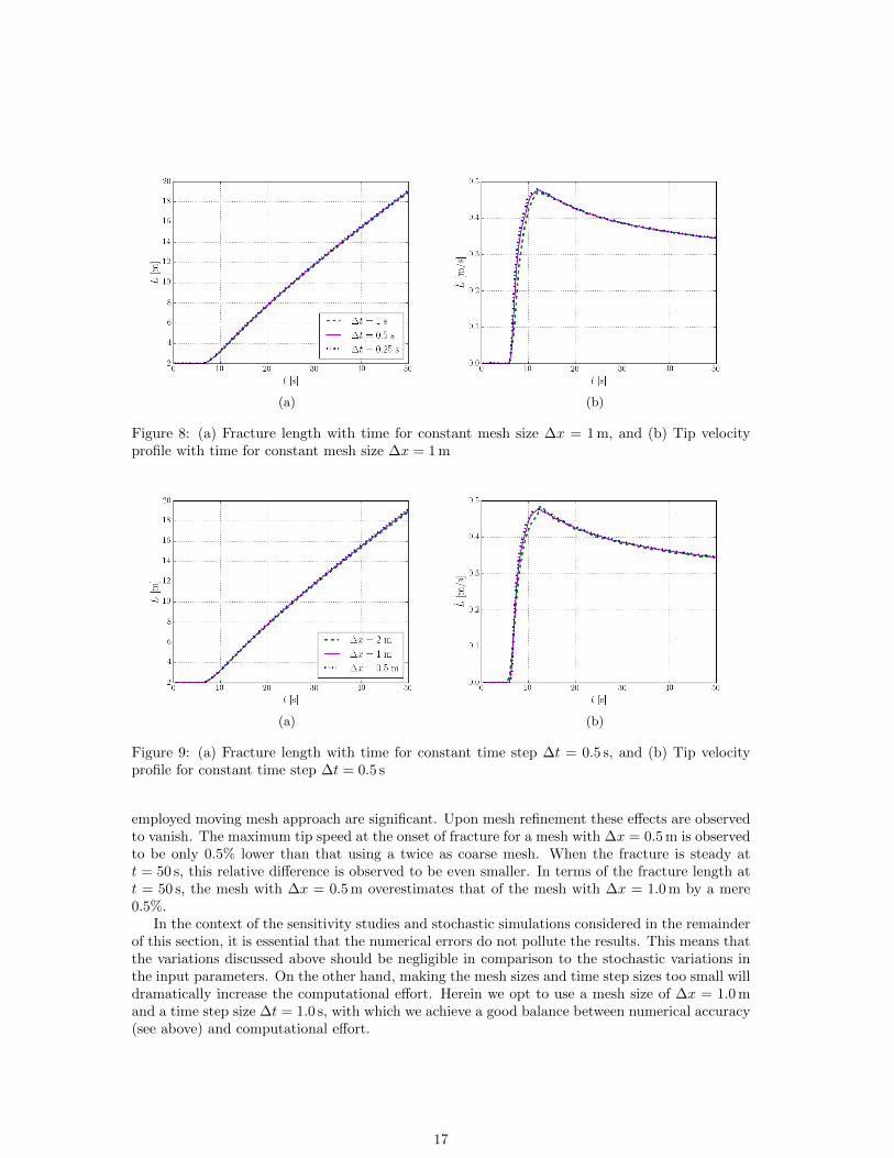
(a) (b)

Figure 8: (a) Fracture length with time for constant mesh size ∆x = 1 m, and (b) Tip velocityprofile with time for constant mesh size ∆x = 1 m

(a) (b)

Figure 9: (a) Fracture length with time for constant time step ∆t = 0.5 s, and (b) Tip velocityprofile for constant time step ∆t = 0.5 s

employed moving mesh approach are significant. Upon mesh refinement these effects are observedto vanish. The maximum tip speed at the onset of fracture for a mesh with ∆x = 0.5 m is observedto be only 0.5% lower than that using a twice as coarse mesh. When the fracture is steady att = 50 s, this relative difference is observed to be even smaller. In terms of the fracture length att = 50 s, the mesh with ∆x = 0.5 m overestimates that of the mesh with ∆x = 1.0 m by a mere0.5%.

In the context of the sensitivity studies and stochastic simulations considered in the remainderof this section, it is essential that the numerical errors do not pollute the results. This means thatthe variations discussed above should be negligible in comparison to the stochastic variations inthe input parameters. On the other hand, making the mesh sizes and time step sizes too small willdramatically increase the computational effort. Herein we opt to use a mesh size of ∆x = 1.0 mand a time step size ∆t = 1.0 s, with which we achieve a good balance between numerical accuracy(see above) and computational effort.

17

(a) (b)

Figure 10: (a) Fracture length and aperture with different plane strain moduli, and (b) Fracturegeometry profile with different plane strain moduli

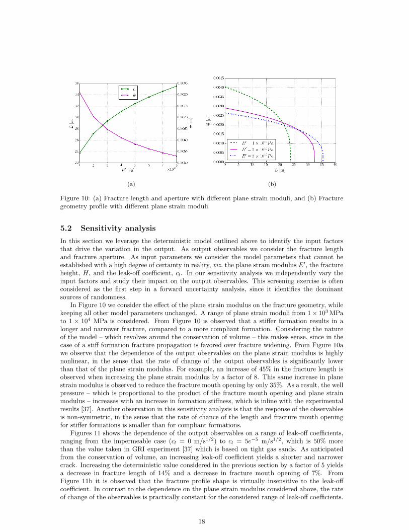
5.2 Sensitivity analysis

In this section we leverage the deterministic model outlined above to identify the input factorsthat drive the variation in the output. As output observables we consider the fracture lengthand fracture aperture. As input parameters we consider the model parameters that cannot beestablished with a high degree of certainty in reality, viz. the plane strain modulus E′, the fractureheight, H, and the leak-off coefficient, cl. In our sensitivity analysis we independently vary theinput factors and study their impact on the output observables. This screening exercise is oftenconsidered as the first step in a forward uncertainty analysis, since it identifies the dominantsources of randomness.

In Figure 10 we consider the effect of the plane strain modulus on the fracture geometry, whilekeeping all other model parameters unchanged. A range of plane strain moduli from 1× 103 MPato 1 × 104 MPa is considered. From Figure 10 is observed that a stiffer formation results in alonger and narrower fracture, compared to a more compliant formation. Considering the natureof the model – which revolves around the conservation of volume – this makes sense, since in thecase of a stiff formation fracture propagation is favored over fracture widening. From Figure 10awe observe that the dependence of the output observables on the plane strain modulus is highlynonlinear, in the sense that the rate of change of the output observables is significantly lowerthan that of the plane strain modulus. For example, an increase of 45% in the fracture length isobserved when increasing the plane strain modulus by a factor of 8. This same increase in planestrain modulus is observed to reduce the fracture mouth opening by only 35%. As a result, the wellpressure – which is proportional to the product of the fracture mouth opening and plane strainmodulus – increases with an increase in formation stiffness, which is inline with the experimentalresults [37]. Another observation in this sensitivity analysis is that the response of the observablesis non-symmetric, in the sense that the rate of chance of the length and fracture mouth openingfor stiffer formations is smaller than for compliant formations.

Figures 11 shows the dependence of the output observables on a range of leak-off coefficients,ranging from the impermeable case (cl = 0 m/s1/2) to cl = 5e−5 m/s1/2, which is 50% morethan the value taken in GRI experiment [37] which is based on tight gas sands. As anticipatedfrom the conservation of volume, an increasing leak-off coefficient yields a shorter and narrowercrack. Increasing the deterministic value considered in the previous section by a factor of 5 yieldsa decrease in fracture length of 14% and a decrease in fracture mouth opening of 7%. FromFigure 11b it is observed that the fracture profile shape is virtually insensitive to the leak-offcoefficient. In contrast to the dependence on the plane strain modulus considered above, the rateof change of the observables is practically constant for the considered range of leak-off coefficients.

18

(a) (b)

Figure 11: (a) Fracture length and aperture with different leak-off coefficient, and (b) Fracturegeometry profile with leak-off coefficient

(a) (b)

Figure 12: (a) Fracture length and aperture with different fracture height, and (b) Fracturegeometry profile with diferent fracture height

In Figures 12 the variation of the output observables for fracture heights ranging from 25 mto 95 m is observed. Doubling the fracture height from 25 m reduces the fracture mouth openingby 15% and the fracture length by 44%. As expected from volume conservation (where in thisparticular case leak-off effects are not pronounced) the product of these two observables is ap-proximately reduced by a factor of two. The direct impact of the fracture height on the volumeconservation model results in a strong sensitivity of the output observables. The non-symmetry ofthe response observables is consistent with the expected behavior in the extreme cases, for whicha extremely large height should yield a very short and narrow crack, and a extremely small height(which is a violation of the model assumptions) should yield an extremely long and wide fracture.

5.3 Stochastic setting

In this section we present the results of the Monte Carlo simulations. In Section 5.3.1 we firststudy the stochastic results for the case where each of the uncertain input parameters is variedindependently, which closely connects this section to the sensitivity analysis presented above. Thestochastic analysis presented here provides additional insights into the evolution of the randomness

19

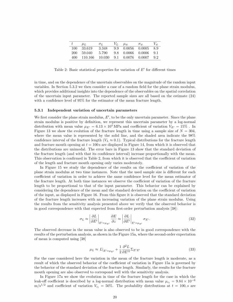
t µL σL VL µw σw Vw100 33.619 3.348 9.9 0.0056 0.0005 8.9200 59.040 5.790 9.8 0.0066 0.0006 9.1400 110.166 10.030 9.1 0.0076 0.0007 9.2

Table 2: Basic statistical properties for variation of E′ for different times

in time, and on the dependence of the uncertain observables on the magnitude of the random inputvariables. In Section 5.3.2 we then consider a case of a random field for the plane strain modulus,which provides additional insights into the dependence of the observables on the spatial correlationof the uncertain input parameter. The reported sample sizes are all based on the estimate (24)with a confidence level of 95% for the estimator of the mean fracture length.

5.3.1 Independent variation of uncertain parameters

We first consider the plane strain modulus, E′, to be the only uncertain parameter. Since the planestrain modulus is positive by definition, we represent this uncertain parameter by a log-normaldistribution with mean value µE′ = 6.13 × 104 MPa and coefficient of variation VE′ = 15% . InFigure 13 we show the evolution of the fracture length in time using a sample size of N = 304,where the mean value is represented by the solid line, and the shaded area indicate the 98%confidence interval of the fracture length (VL ≈ 0.1). Typical distributions for the fracture lengthand fracture mouth opening at t = 100 s are displayed in Figure 14, from which it is observed thatthe distributions are unimodal. The error bars in Figure 13 show that the standard deviation ofthe fracture length (and with that its confidence interval) increase proportionally with the mean.This observation is confirmed in Table 2, from which it is observed that the coefficient of variationof the length and fracture mouth opening only varies moderately.

In Figure 15 we study the dependence of the results on the coefficient of variation of theplane strain modulus at two time instances. Note that the used sample size is different for eachcoefficient of variation in order to achieve the same confidence level for the mean estimator ofthe fracture length. At both time instances we observe the coefficient of variation of the fracturelength to be proportional to that of the input parameter. This behavior can be explained byconsidering the dependence of the mean and the standard deviation on the coefficient of variationof the input, as displayed in Figure 16. From this figure it is observed that the standard deviationof the fracture length increases with an increasing variation of the plane strain modulus. Usingthe results from the sensitivity analysis presented above we verify that the observed behavior isin good correspondence with that expected from first-order perturbation analysis [38]:

σL ≈∣∣∣∣ ∂L∂E′

∣∣∣∣E′=µE′

∂E

∂z≈∣∣∣∣ ∂L∂E′

∣∣∣∣E′=µE′

σE′ . (32)

The observed decrease in the mean value is also observed to be in good correspondence with theresults of the perturbation analysis, as shown in the Figure 15a, where the second-order expectationof mean is computed using [38]

µL ≈ L|E′=µE′ +1

2

∂2L

∂E′2ΣE′E′ (33)

For the case considered here the variation in the mean of the fracture length is moderate, as aresult of which the observed behavior of the coefficient of variation in Figure 15a is governed bythe behavior of the standard deviation of the fracture length. Similarly, the results for the fracturemouth opening are also observed to correspond well with the sensitivity analysis.

In Figure 17a we show the evolution in time of the fracture length for the case in which theleak-off coefficient is described by a log-normal distribution with mean value µcl = 9.84 × 10−6

m/s1/2 and coefficient of variation Vcl = 50%. The probability distributions at t = 100, s are

20

Figure 13: Error bar of fracture length evolution with time

(a) (b)

Figure 14: (a) Histogram of L for 50% variation of E′, and (b) Histogram for w for 50% variationof E′

(a) (b)

Figure 15: (a) L and w with different variation of E′ at t = 100 s and (b) L and w with differentvariation of E′ at t = 500 s

21

(a) (b)

Figure 16: (a)µL and µw with different variation of E′ at t = 100 s, and (b) σL and σw withdifferent variation E′ at t = 100 s

(a) (b)

Figure 17: (a) Error bar of L with time for cl, and (b) Error bar of L with time for H

shown in Figure 18. In Figure 19 we study the relation between the coefficients of variation ofthe observables and that of the leak-off coefficient at two time instances, where the sample sizeshave been selected in accordance with the confidence level of the mean estimator of the fracturelength. It is observed that the coefficients of variation of the output observables are not changingsignificantly in time. The observed relation between the coefficients of variation of the input andoutput is explained by the fact that the mean value is effected minimally by the coefficient ofvariation of the leak-off coefficient, while the standard deviation increases proportionally withit. From Figure 19 it is observed that the behavior of the mean and standard deviations of theobservables is in good agreement (with a maximum of 3% variation which can be attributed to theapproximations made while computing perturbation results, see Appendix 4)with the perturbationresults following from the sensitivity analysis.

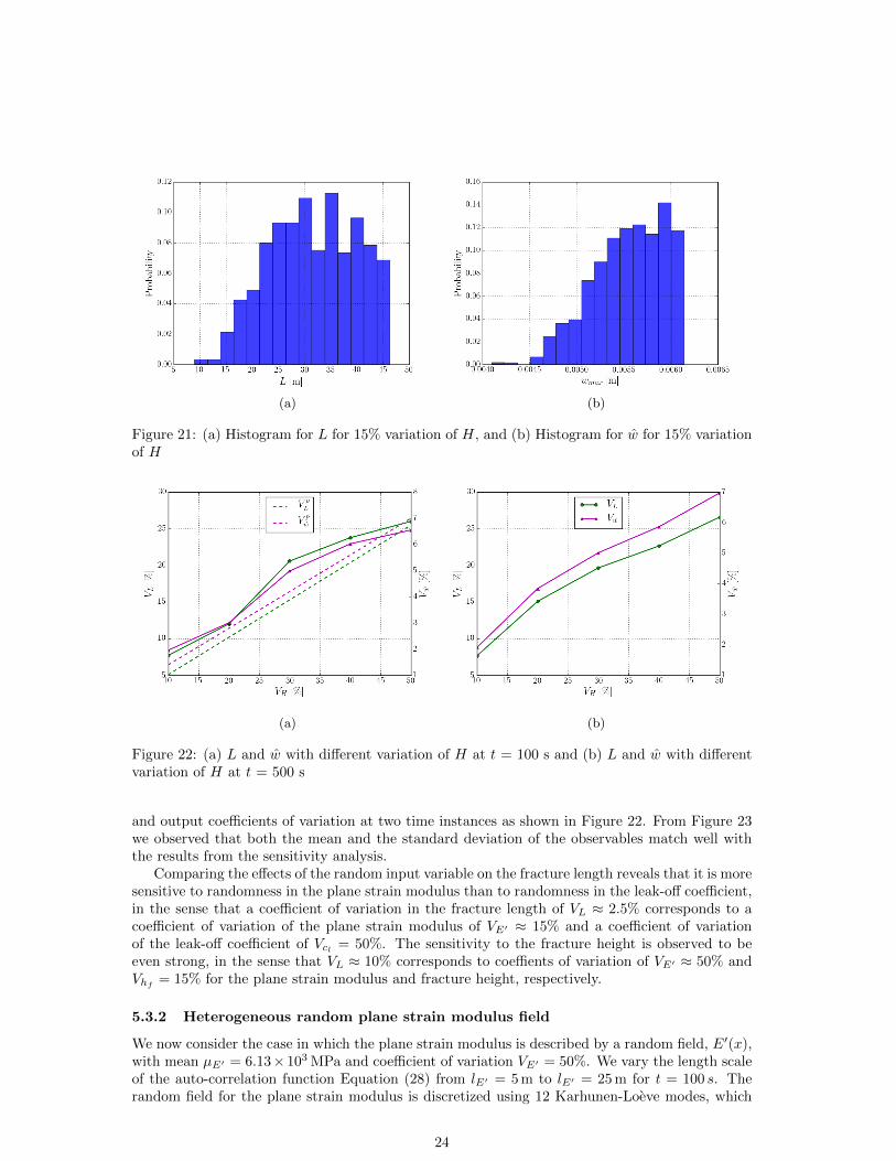
We finally consider the independent random variation of the fracture height, which is repre-sented by a log-normal distribution with mean µH = 51.8 m and coefficient of variation VH = 50%.A sample size of N = 553 (with a confidence level of 95% ) is selected to compute the time evolu-tion of the fracture length as shown in Figure 17b, for which two of the probability distributionsat time t = 100 s are shown in Figure 21. The coefficient of variation is observed not to be subjectto significant changes in time, which is confirmed by comparison of the relation between the input

22

(a) (b)

Figure 18: (a) Histogram for L for 50% variation of cl, and (b) Histogram for w for 50% variationof cl

(a) (b)

Figure 19: L and w with different variation of cl at t = 100 s and (b) L and w with differentvariation of cl at t = 500 s

(a) (b)

Figure 20: (a)µL and µw with different variation of cl at t = 100 s, and (b) σL and σw withdifferent variation cl at t = 100 s

23

(a) (b)

Figure 21: (a) Histogram for L for 15% variation of H, and (b) Histogram for w for 15% variationof H

(a) (b)

Figure 22: (a) L and w with different variation of H at t = 100 s and (b) L and w with differentvariation of H at t = 500 s

and output coefficients of variation at two time instances as shown in Figure 22. From Figure 23we observed that both the mean and the standard deviation of the observables match well withthe results from the sensitivity analysis.

Comparing the effects of the random input variable on the fracture length reveals that it is moresensitive to randomness in the plane strain modulus than to randomness in the leak-off coefficient,in the sense that a coefficient of variation in the fracture length of VL ≈ 2.5% corresponds to acoefficient of variation of the plane strain modulus of VE′ ≈ 15% and a coefficient of variationof the leak-off coefficient of Vcl = 50%. The sensitivity to the fracture height is observed to beeven strong, in the sense that VL ≈ 10% corresponds to coeffients of variation of VE′ ≈ 50% andVhf = 15% for the plane strain modulus and fracture height, respectively.

5.3.2 Heterogeneous random plane strain modulus field

We now consider the case in which the plane strain modulus is described by a random field, E′(x),with mean µE′ = 6.13× 103 MPa and coefficient of variation VE′ = 50%. We vary the length scaleof the auto-correlation function Equation (28) from lE′ = 5 m to lE′ = 25 m for t = 100 s. Therandom field for the plane strain modulus is discretized using 12 Karhunen-Loeve modes, which

24

(a) (b)

Figure 23: (a) µL and µw with different variation of H at t = 100 s, and (b) σL and σw withdifferent variation H at t = 100 s

is sufficient for the representation of the random field corresponding to the smallest correlationlength considered. In Table 3 the statistical moments of the observables are collected based on aMonte-Carlo simulation with N = 384, which is in accordance with a 95% confidence level for themean estimator in the fracture length.

The most notable observation from the results in Table 3 is that the coefficient of variationof the output observables is significantly higher than in the case of a homogeneous plane strainmodulus with equal coefficient of variation (see Table 3). To better understand this observation,in Figure 24 we perform a closer inspection of the realizations that lead to Table 3. In the rowsof this figure we collect the Monte-Carlo results for the correlation lengths reported in Table 3,starting with the smallest correlation length on top. In the second and third column we showthe probability distributions for the fracture length and the fracture mouth opening. In the firstcolumn we show the plane strain modulus field that leads to three distinct realizations in thesample, viz. the smallest fracture length, the largest fracture length, and the fracture lengthclosest to the mean value.

We observe that the realizations of the plane strain modulus field that lead to the smallestfracture lengths in all cases correspond to the situation in which the elastic modulus is very smallnear the well. When this happens the injected fluid causes fracture widening near the well, ratherthan fracture propagation into the formation. More generally, in the case of heterogeneous fields,local zones in which the formation is very compliant can lead to blockage of propagation, as theinjected fluid volume can be locally accumulated in this zone. Long fractures are obtained in thecase that the plane strain modulus is large near the well, and high (in a spatially averaged sense)compared to the mean value. In such situations the blockage of propagation due to a compliantzone does not occur.

In terms of the dependence of the results on the correlation length it is observed that the meanfracture length decreases as the correlation length decreases. This is explained by the fact that inthe case of a smaller correlation length, the chance of a locally compliant zone in the formationincreases. The blockage of propagation in such zones is then more frequent, which leads to areduction in fracture length expectation. From Table 3 we moreover observe a moderate increasein coefficient of variation of the fracture length as the correlation length increases.

From the distributions of the fracture mouth opening in Figures 24c1-24c5 we observe a notabledifference in comparison to those for the homogeneous random plane strain modulus case (Fig-ure 14b). In the homogeneous case there exists a strong correlation between the fracture lengthand the fracture mouth opening, in the sense that long cracks are narrow by virtue of the fact thattheir volume is similar (assuming leak-off effects to be limited). Figure 10 in the sensitivity studyclearly confirms this observation. Although the fracture length and fracture width in the case

25

a1 b1 c1

a2 b2 c2

a3 b3 c3

a4 b4 c4

a5 b5 c5

Figure 24: (a1-a5) Examples of realization for lE′ = (5, 10, 15, 20, 25)m respectively (b1-b5) His-togram for fracture length for lE′ = (5, 10, 15, 20, 25)m respectively and (c1-c5) Histogram formaximum aperture for lE′ = (5, 10, 15, 20, 25)m respectively

26

lE′ [m] µL [m] σL [m] VL[%] µw [m] σw [m] Vw[%]5 27.545 6.682 24.3 0.0071 0.0030 42.310 28.496 7.177 25.2 0.0078 0.0041 52.615 29.319 6.204 21.2 0.0075 0.0037 49.320 29.735 6.601 22.2 0.0074 0.0029 39.225 31.091 6.158 19.8 0.0067 0.0021 31.3

Table 3: Basic statistical properties for 50% variation of E′ for different lE′ for t = 100 s

(a) (b)

Figure 25: (a)xf and w with different variation of E′ at t = 100 s for lE′ = 20 m and (b) xf andw with different variation of E′ at t = 500 s for lE′ = 20 m

of a heterogeneous field are not uncorrelated, the fracture mouth opening is strongly influencedby the local plane strain modulus near the well. Since the fracture opening in the PKN modeldepends locally on the plane strain modulus, the log-normal distribution of the plane strain mod-ulus reflects directly on that of the fracture mouth opening, as can be seen in the third column ofFigures 24c1-24c5. The sensitivity of the fracture mouth opening to local variations in the planestrain modulus field also results in coefficients of variation that are significantly higher than thosein the homogeneous case.

6 Conclusions

We have presented a sampling-based stochastic analysis of the hydraulic fracturing process basedon the Perkins-Kern-Nordgren (PKN) model. The consideration of this model is motivated bythe fact that in the deterministic case high-accuracy solutions can be computed with limitedcomputational effort, which makes its application in the context of direct Monte Carlo samplingpractical. Although this model significantly simplifies the hydraulic fracturing process, it bearspractical relevance, especially for fractures in the viscosity-dominated regime. A limitation of themodel of particular relevance in this study results from the local elasticity relation in the PKNmodel, which restricts its application to low-frequency spatial variations of the model parameters.

In order to compute high-fidelity solutions that do not pollute stochastic analyses with numeri-cal errors, a moving-mesh finite element method is developed. The employed backward-Euler timeintegration scheme is supplemented with a sub-iteration technique, such that the mesh propagationrelation becomes implicit. The non-linearity of the model is solved using Newton iterations.

We have performed detailed mesh size and time integration step convergence studies. We havefound that in order to attain solutions with acceptable accuracy in the context of the stochastic

27

(a) (b)

Figure 26: (a) )µxf and µwmax with different variation of E′ at t = 100 s for lE′ = 20 m, and (b)σxf and σwmax with different variation E′ at t = 100 s for lE′ = 20 m

analysis considered herein, the finite element methodology had to be enhanced. First, the globalconservation of volume was found to be significantly violated due to the highly non-linear characterof the model. The observed loss of volume led to significant underestimation of the fracture length.To circumvent this problem, volume conservation was enforced by means of a Lagrange multiplierapproach. Second, the weakly singular behavior of the fracture opening and pressure at the tipwas found to be troublesome in the case of a standard finite element basis. On one hand theimproper representation of the singularity by the basis required the use of an ad hoc tip velocityrelation. On the other hand, the mesh resolution of the uniform finite element mesh was foundto be insufficient. These issues were resolved by enrichment of the standard finite element spacewith a singular tip function.

Our finite element simulations show very good agreement with results reported in literaturefor a realistic test case. The sensitivity of the fracture evolution process with respect to variousrandom input parameters was studied. From the conducted direct Monte Carlo simulations it wasfound that the mean and standard deviation of the fracture length and fracture mouth openingcorrespond well to those values obtained using perturbation theory. This observation conveys that– at least for the test case considered – linearization of the model provides meaningful informationon the behavior of the stochastic moments, despite the complexity of the model and its solutionprocedure.

To demonstrate the suitability of the developed methodology for studying random hetero-geneities in formation properties we have considered a test case in which the formation stiffnesswas described by a random field. The random dimension was discretized using a Karhunen-Loeveexpansion, while the spatial dimension was discretized using a linear finite element mesh on abackground domain. The sampling results demonstrate that the response uncertainty is amplifiedby the heterogeneous character of the random material property field. For the fracture lengththis is explained by the fact that fracture propagation is sensitive to local variations in the elasticproperties of the formation. For the fracture mouth opening an even stronger amplification isobserved as a consequence of the fact that the fracture opening is directly related to the materialproperty. Although this observation can be explained well based on the structure of the PKNmodel, it requires further study to understand to what extend a similar conclusion can be drawnfor more rich hydraulic fracturing models.

Although the results presented herein provide excellent insight into the primary characteristicsof the stochastic behavior of the hydraulic fracturing process, it is evident that more detailedinformation can be obtained by a more versatile model and simulation strategy. In particularthe PKN model does not rely on a fracture mechanics model based on the material’s fracturetoughness, which restricts the scope of this work to fractures in the viscosity-dominated regime.

28

When considering uncertainty quantification using physically richer models it will remain key tonot pollute the results with numerical errors, which will inevitably lead to computationally veryexpensive Monte Carlo methods. The use of alternative stochastic techniques, such as e.g. theperturbation method can be expected to yield meaningful results at a much lower cost than directMonte Carlo sampling.

29

A Karhonen-Loeve Expansion and its discretizion using fi-nite elements

Here, we discuss the discretization of Karhunen-Loeve expansion in a finite element setting. TheKarhunen Loeve expansion of a normal random field is expressed as:

G(x) = µG +

∞∑i=1

gi(x)zi (34)

where zi are stochastic dependence or uncorrelated standard normal variables and gi(x) are theeigen functions of the following integral equation [38].∫

Ω

∑EE

(x1,x2)gi(x2)dx2 = λigi(x1) (35)

where∑EE(x1,x2) are covariance kernal of the deterministic function of the random field G(x).

Furthermore, the random process can be expressed as a direct sum of orthogonal projections ofthe basis functions gi(x) which are proportional to the corresponding eigenvalues.∫

Ω

gi(x)2 = λi (36)

Thus, it has a spectral decomposition

∑EE

(x1,x2) =

∞∑i=1

gi(x1)gi(x2) (37)

The eigenvectors and eigenfunctions can be solved using finite elements. The eigenfunctionsare represented in terms of the shape functions. The infinite number of eigenfunctions are approx-imated to finite number and are obtained by expanding in finite elements and transforming theeigenvalue problem into an algebraic eigenvalue problem [39].

gi(x) =

m∑j=1

N j(x)Φji = N(x)TΦi (38)

Discretization the integral equation we get,∫Ω

∑EE

(x1,x2)N(x2)TΦidx2 = λiN(x1)TΦi (39)

Galerkin formulation results in generalized matrix eigen value problem of the form

AΦi = λiBΦi (40)

Thus, random field in finite elements for a normal field can be written as

G(x) = µG +

m∑i=1

Φizi (41)

30

B Length and maximum aperture of the fracture at differ-ent times

We consider the benchmark case studied by Warpinski et al.[37], which is based on a staged-field experiment of the Gas Research Institute [37, p. 26]. The considered model parameters areassembled in Table 1. The injection rate is gradually increased until the indicated value, and thenheld constant for 200 minutes. The material parameters resemble that of a tight gas sand reservoir,for which spurt losses are omitted. The shown results are based on a mesh size of ∆x = 1 m anda time step size of ∆t = 1 s and rounded off to 4 significant digits.

Time Height L w(sec) (m) (m) (m)0 51.8 2.0000 0.00371200 51.8 246.1651 0.00892400 51.8 421.3913 0.01013600 51.8 575.4035 0.01094800 51.8 716.5376 0.01146000 51.8 848.7358 0.01197200 51.8 974.0853 0.01228400 51.8 1093.9648 0.01269600 51.8 1209.3184 0.012910400 51.8 1320.8104 0.013112000 51.8 1428.9438 0.0134

Table 4: Output for different times

31

C Perturbation results

Using the results from the sensitivity analysis from presented above we verify that the observedbehavior is in good correspondence with that expected from first-order perturbation analysis [40]:

σL ≈∣∣∣∣ ∂L∂E′

∣∣∣∣E′=µE′

∂E

∂z≈∣∣∣∣ ∂L∂E′

∣∣∣∣E′=µE′

σE′ . (42)

The observed decrease in the mean value is also observed to be in good correspondence with theresults of the perturbation analysis, as shown in the Figure 16a, where the second-order expectationof mean is computed using the following equation (43)

µL ≈ L|E′=µE′ +1

2

∂2L

∂E′2ΣE′E′ (43)

For all the calulations, we compute the first dervatives and second dervatives using finite dif-ferences scheme.

In case of E′, the corresponding values of length and width were from 5×1010 Pa and 7×1010

Pa. We get the following

VL = 0.199× VE′

Vwmax = 0.239× VE′

In case of cl, the corresponding values of length and width were from 9 × 10−6 m/s1/2 and1× 10−5 m/s1/2. We get the following

VL = 0.0381× Vcl

Vwmax = 0.0352× VclIn case of H, the corresponding values of length and width were from 45 m and 60 m. We get

the following

VL = 0.51× Vhf

Vwmax = 0.14× Vhf

32

References

[1] LR Kern TK Perkins. Widths of hydraulic fractures. Journal of Petroleum Technology, 1961.

[2] RP Nordgren. Propagation of vertical hydraulic fractures. Society of Petroleum EngineersJournal, 1972.

[3] Ian N. Sneddon. A note on the problem of the penny-shaped crack. Mathematical Proceedingsof the Cambridge Philosophical Society, 61(2):609611, 1965.

[4] INa Sneddon. The distribution of stress in the neighbourhood of a crack in an elastic solid.In Proceedings of the Royal Society of London A: Mathematical, Physical and EngineeringSciences, volume 187, pages 229–260. The Royal Society, 1946.

[5] A Khristianovic Zheltov et al. 3. formation of vertical fractures by means of highly viscousliquid. In 4th World Petroleum Congress. World Petroleum Congress, 1955.

[6] Paul Meakin, G Li, LM Sander, E Louis, and F Guinea. A simple two-dimensional model forcrack propagation. Journal of Physics A: Mathematical and General, 22(9):1393, 1989.

[7] J Geertsma, F De Klerk, et al. A rapid method of predicting width and extent of hydraulicallyinduced fractures. Journal of Petroleum Technology, 21(12):1–571, 1969.

[8] Antonin Settari, Michael P Cleary, et al. Development and testing of a pseudo-three-dimensional model of hydraulic fracture geometry. SPE Production Engineering, 1(06):449–466, 1986.

[9] ER Simonson, AS Abou-Sayed, RJ Clifton, et al. Containment of massive hydraulic fractures.Society of Petroleum Engineers Journal, 18(01):27–32, 1978.

[10] J Adachi, E Siebrits, A Peirce, and J Desroches. Computer simulation of hydraulic fractures.International Journal of Rock Mechanics and Mining Sciences, 44(5):739–757, 2007.

[11] Y. Kovalyshen and E. Detournay. A reexamination of the classical pkn model of hydraulicfracture. 2010.

[12] AP Peirce and EDUARD Siebrits. An eulerian finite volume method for hydraulic fractureproblems. Finite volumes for complex applications IV, ISTE, London, pages 655–664, 2005.

[13] S.H. Advani and J. Lee. Finite element model simulations associated with hydraulic fractur-ing. Society of Petroleum Engineers Journal, 1982.

[14] Axel KL Ng and John C Small. A case study of hydraulic fracturing using finite elementmethods. Canadian Geotechnical Journal, 36(5):861–875, 1999.

[15] Magnus Wangen. Finite element modeling of hydraulic fracturing on a reservoir scale in 2d.Journal of Petroleum Science and Engineering, 77(3):274 – 285, 2011.

[16] Benjamin Ganis, Mark E. Mear, A. Sakhaee-Pour, Mary F. Wheeler, and Thomas Wick.Modeling fluid injection in fractures with a reservoir simulator coupled to a boundary elementmethod. Computational Geosciences, 18(5):613–624, Oct 2014.

[17] A Munjiza, DRJ Owen, and N Bicanic. A combined finite-discrete element method in transientdynamics of fracturing solids. Engineering computations, 12(2):145–174, 1995.

[18] Brice Lecampion. An extended finite element method for hydraulic fracture problems. Com-munications in Numerical Methods in Engineering, 25(2):121–133, 2009.

[19] A. Mikelic, M.F. Wheeler, and T. Wick. Phase-field modeling of a fluid-driven fracture in aporoelastic medium. Computational Geosciences, 19(6):1171–1195, Dec 2015.

33

[20] Emmanuel Detournay. Mechanics of hydraulic fractures. Annual Review of Fluid Mechanics,2016.

[21] DJ YOUN and DV Griffiths. Stochastic analysis of hydraulic fracture propagation usingthe extended finite element method and random field theory. In Integrating Innovations ofRock Mechanics: Proceedings of the 8th South American Congress on Rock Mechanics, 15–18November 2015, Buenos Aires, Argentina, page 189. IOS Press, 2015.

[22] Merle E Hanson, Ronald J Shaffer, Gordon D Anderson, et al. Effects of various parameterson hydraulic fracturing geometry. Society of Petroleum Engineers Journal, 21(04):435–443,1981.

[23] GM Zhang, H Liu, J Zhang, HA Wu, and XX Wang. Three-dimensional finite elementsimulation and parametric study for horizontal well hydraulic fracture. Journal of PetroleumScience and Engineering, 72(3):310–317, 2010.

[24] LF Kemp. Study of nordgren’s equation of hydraulic fracturing. SPE Production Engineering,1990.

[25] P. Valko and M.J. Economides. Hydraulic fracturing. 1985.

[26] Robert W. Zimmerman and In-Wook Yeo. Fluid flow in rock fractures: From the navier-stokesequations to the cubic law. Dynamics of Fluids in Fractured Rock, 2013.

[27] George Keith Batchelor. An introduction to fluid dynamics. Cambridge university press,2000.

[28] CR Fast GC Howard. Optimum fluid characteristics for fracture extension. Drilling andproduction practice, 1957.

[29] M. Lowengrub. A note on griffith cracks. Proceedings of the Edinburgh Mathematical Society,15(2):131134, 1966.

[30] A. H. England and A. E. Green. Some two-dimensional punch and crack problems in classicalelasticity. Mathematical Proceedings of the Cambridge Philosophical Society, 59(2):489500,1963.

[31] JI Adachi and E Detournay. Self-similar solution of a plane-strain fracture driven by a power-law fluid. International Journal for Numerical and Analytical Methods in Geomechanics,26(6):579–604, 2002.

[32] D Garagash and E Detournay. The tip region of a fluid-driven fracture in an elasticmedium. Transactions-American Society of Mechanical Engineers Journal of Applied Me-chanics, 67(1):183–192, 2000.

[33] Jens M Melenk and Ivo Babuska. The partition of unity finite element method: basic theoryand applications. Computer methods in applied mechanics and engineering, 139(1-4):289–314,1996.

[34] Jerzy Neyman. Outline of a theory of statistical estimation based on the classical theory ofprobability. Philosophical Transactions of the Royal Society of London. Series A, Mathemat-ical and Physical Sciences, 236(767):333–380, 1937.

[35] John Francis Kenney. Mathematics of statistics. D. Van Nostrand Company Inc; Toronto;Princeton; New Jersey; London; New York,; Affiliated East-West Press Pvt-Ltd; New Delhi,2013.

[36] Elaine Barker, William Barker, William Burr, William Polk, and Miles Smid. Recommenda-tion for key management part 1: General (revision 3). NIST special publication, 800(57):1–147,2012.

34

[37] N.R. Warpinki, Z.A. Moschovidis, C.D. Parker, and I.S. Abou-Sayed. Is: Comparison studyof hydraulic fracturing models: Test case - gri-staged experiment no. 3. SPE ProductionEngineering and Facilities, 1994.

[38] Miguel A. Gutirrez and Steen Krenk. Stochastic finite element methods. 2004.

[39] R. G. Ghanem and P. D. Spanos. Spectral techniques for stochastic finite elements. Archivesof Computational Methods in Engineering, 4(1):63–100, Mar 1997.

[40] Gutirrez MA and Krenk S. Encyclopedia of Computational Mechanics, volume 2. John Wiley& Sons, 2004.

35