Embed Size (px)
Citation preview
3/26/2013
Fisher’s Equation: Analysis and numerical solutions Author:
Mandeep Singh
Page 1 of 26
Contents Introduction ............................................................................................................................................................................ 2
Stability Analysis ..................................................................................................................................................................... 2
Numerics ................................................................................................................................................................................. 3
Forward Euler Method (Results) ............................................................................................................................................. 5
Runge-Kutta Method, 4th Order (Results) ............................................................................................................................... 8
Trapezoidal Method (Results) ............................................................................................................................................... 11
Backwards Euler Method (Results) ....................................................................................................................................... 14
Forward Euler Method (MATLAB Code) ............................................................................................................................... 17
Runge-Kutta Method, 4th Order (MATLAB Code) .................................................................................................................. 18
Trapezoidal Method (MATLAB Code) ................................................................................................................................... 20
Backwards Euler Method (MATLAB Code) ............................................................................................................................ 23
References ............................................................................................................................................................................ 26
Page 2 of 26
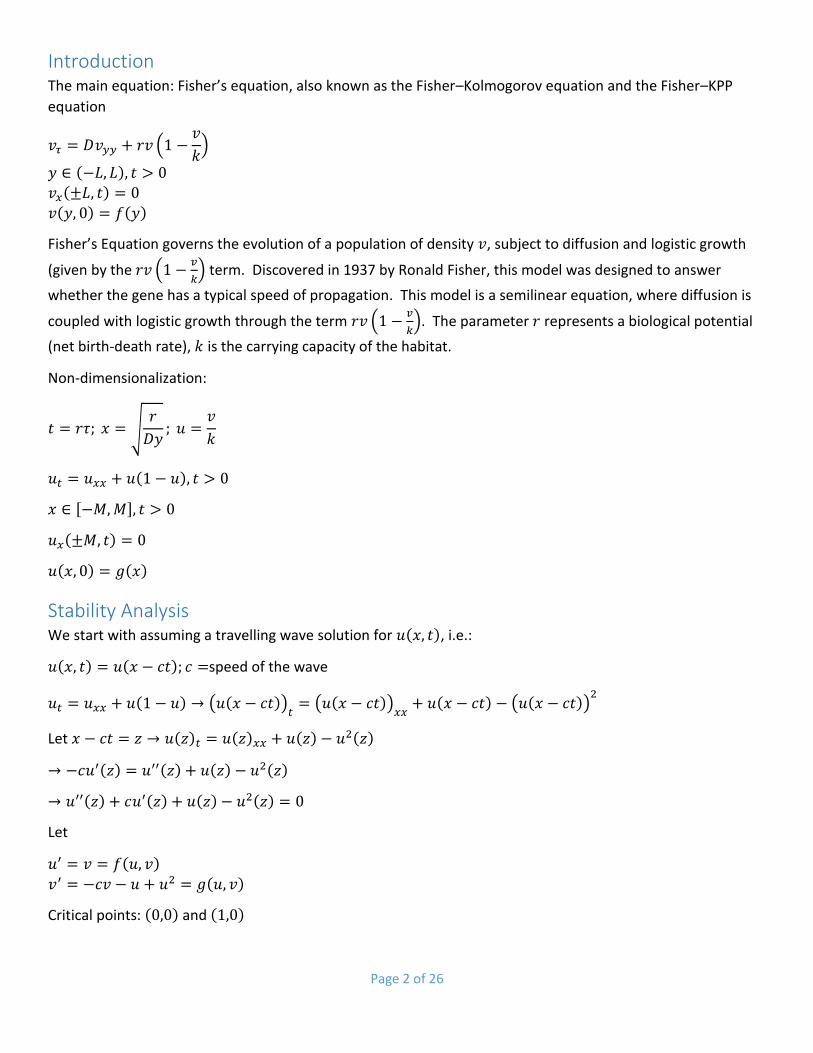
Introduction The main equation: Fisher’s equation, also known as the Fisher–Kolmogorov equation and the Fisher–KPP
equation
𝑣𝜏 = 𝐷𝑣𝑦𝑦 + 𝑟𝑣 (1 −𝑣
𝑘)
𝑦 ∈ (−𝐿, 𝐿), 𝑡 > 0
𝑣𝑥(±𝐿, 𝑡) = 0
𝑣(𝑦, 0) = 𝑓(𝑦)
Fisher’s Equation governs the evolution of a population of density 𝑣, subject to diffusion and logistic growth
(given by the 𝑟𝑣 (1 −𝑣
𝑘) term. Discovered in 1937 by Ronald Fisher, this model was designed to answer
whether the gene has a typical speed of propagation. This model is a semilinear equation, where diffusion is
coupled with logistic growth through the term 𝑟𝑣 (1 −𝑣
𝑘). The parameter 𝑟 represents a biological potential
(net birth-death rate), 𝑘 is the carrying capacity of the habitat.
Non-dimensionalization:
𝑡 = 𝑟𝜏; 𝑥 = √𝑟
𝐷𝑦; 𝑢 =
𝑣
𝑘
𝑢𝑡 = 𝑢𝑥𝑥 + 𝑢(1 − 𝑢), 𝑡 > 0
𝑥 ∈ [−𝑀,𝑀], 𝑡 > 0
𝑢𝑥(±𝑀, 𝑡) = 0
𝑢(𝑥, 0) = 𝑔(𝑥)
Stability Analysis
We start with assuming a travelling wave solution for 𝑢(𝑥, 𝑡), i.e.:
𝑢(𝑥, 𝑡) = 𝑢(𝑥 − 𝑐𝑡); 𝑐 =speed of the wave
𝑢𝑡 = 𝑢𝑥𝑥 + 𝑢(1 − 𝑢) → (𝑢(𝑥 − 𝑐𝑡))𝑡= (𝑢(𝑥 − 𝑐𝑡))
𝑥𝑥+ 𝑢(𝑥 − 𝑐𝑡) − (𝑢(𝑥 − 𝑐𝑡))
2
Let 𝑥 − 𝑐𝑡 = 𝑧 → 𝑢(𝑧)𝑡 = 𝑢(𝑧)𝑥𝑥 + 𝑢(𝑧) − 𝑢2(𝑧)
→ −𝑐𝑢′(𝑧) = 𝑢′′(𝑧) + 𝑢(𝑧) − 𝑢2(𝑧)
→ 𝑢′′(𝑧) + 𝑐𝑢′(𝑧) + 𝑢(𝑧) − 𝑢2(𝑧) = 0
Let
𝑢′ = 𝑣 = 𝑓(𝑢, 𝑣)
𝑣′ = −𝑐𝑣 − 𝑢 + 𝑢2 = 𝑔(𝑢, 𝑣)
Critical points: (0,0) and (1,0)
Page 3 of 26
𝐽(𝑢, 𝑣) = (𝑓𝑢 𝑓𝑣𝑔𝑢 𝑔𝑣
) = (0 1
−1 + 2𝑢 −𝑐)
𝐽(0,0) = 𝐽1 = (0 1−1 −𝑐
) ; 𝐽(1,0) = 𝐽2 = (0 11 −𝑐
)
𝜆0,0 =−𝑐 ± √𝑐2 − 4
2
From above we get that the point (0,0) is a stable node for all values greater than or equal to 2 i.e. for 𝑐 ≥ 2
and for 𝑐 = 2, we have a degenerate node. For 𝑐2 < 4, the system is a stable spiral.
𝜆1,0 =−𝑐 ± √𝑐2 + 4
2
From above we get that the point(1,0) is a saddle point because both eigenvalues are real but one is positive
and one is negative.
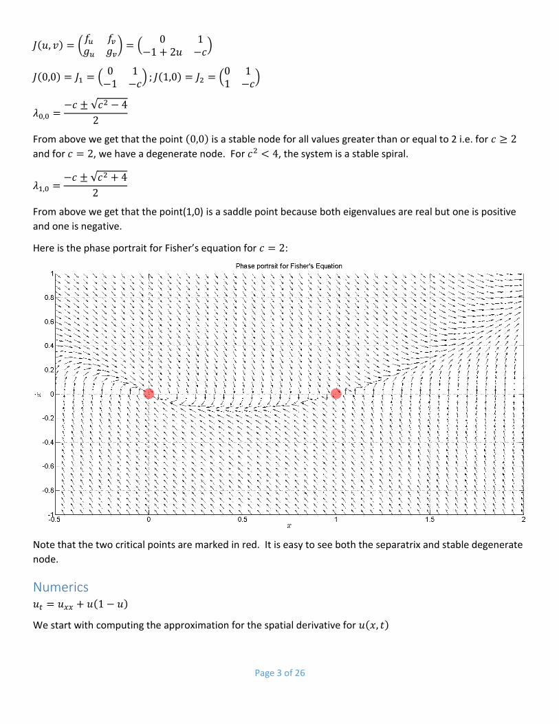
Here is the phase portrait for Fisher’s equation for 𝑐 = 2:
Note that the two critical points are marked in red. It is easy to see both the separatrix and stable degenerate
node.
Numerics 𝑢𝑡 = 𝑢𝑥𝑥 + 𝑢(1 − 𝑢)
We start with computing the approximation for the spatial derivative for 𝑢(𝑥, 𝑡)
Page 4 of 26
𝑢𝑥𝑥(𝑥, 𝑡) ≈𝑢(𝑥 − Δ𝑥, 𝑡) − 2𝑢(𝑥, 𝑡) + 𝑢(𝑥 + Δ𝑥, 𝑡)
(Δ𝑥)2
The purpose of this approximation is to take our nonlinear PDE and approximate it as a nonlinear, time
dependent ODE.
∴, 𝑢𝑡 ≈1
(Δ𝑥)2[𝑢(𝑥 − Δ𝑥, 𝑡) − 2𝑢(𝑥, 𝑡) + 𝑢(𝑥 + Δ𝑥, 𝑡)] + 𝑢(𝑥, 𝑡)(1 − 𝑢(𝑥, 𝑡)) = 𝑓(𝑥, 𝑡) … 1
We can re-write the above equation using indices:
𝑢𝑛 ≈1
(Δ𝑥)2[𝑢(𝑥𝑖−1, 𝑡𝑛) − 2𝑢(𝑥𝑖, 𝑡𝑛) + 𝑢(𝑥𝑖+1, 𝑡𝑛)] + 𝑢(𝑥𝑖, 𝑡𝑛)(1 − 𝑢(𝑥𝑖, 𝑡𝑛)) = 𝑓(𝑥𝑖 , 𝑡𝑛)… 2
Note the subscript on 𝑢 changes from 𝑡 to 𝑛. As 𝑛 is our time index, the above equation is at the time step
𝑡 = 𝑛ℎ, where ℎ = Δ𝑡. In other words, for the given space point, 𝑥𝑖, we calculate the time evolution by
keeping the space index,𝑖, fixed and going to the next time index, 𝑛 + 1. We perform this calculation using
nested loops.
Also, in order to account for the no-flux boundary conditions 𝑢𝑥(±𝑀, 𝑡) = 0, the space points at 𝑖 = 1 and 𝑖 =
𝑁 need to be treated differently. These points are approximated by the following equations:
𝑢𝑛 ≈(−2𝑢(𝑥1, 𝑡𝑛) + 2𝑢(𝑥2, 𝑡𝑛))
(Δ𝑥)2+ 𝑢(𝑥1, 𝑡𝑛)(1 − 𝑢(𝑥1, 𝑡𝑛))… 3
The above equation is at 𝑥 = −𝑀 (left boundary point), and as before, the equation represents the time
evolution of this boundary point at index 𝑖 = 1.
𝑢𝑛 ≈(−2𝑢(𝑥𝑁 , 𝑡𝑛) + 2𝑢(𝑥𝑁−1, 𝑡𝑛))
(Δ𝑥)2+ 𝑢(𝑥𝑁 , 𝑡𝑛)(1 − 𝑢(𝑥𝑁 , 𝑡𝑛))… 4
i.e.:
𝑢𝑛 = 𝑓(𝑥𝑖, 𝑡𝑛) ≈
{
(−2𝑢(𝑥1, 𝑡𝑛) + 2𝑢(𝑥2, 𝑡𝑛))
(Δ𝑥)2+ 𝑢(𝑥1, 𝑡𝑛)(1 − 𝑢(𝑥1, 𝑡𝑛)); 𝑖 = 1
1
(Δ𝑥)2[𝑢(𝑥𝑖−1, 𝑡𝑛) − 2𝑢(𝑥𝑖 , 𝑡𝑛) + 𝑢(𝑥𝑖+1, 𝑡𝑛)] + 𝑢(𝑥𝑖 , 𝑡𝑛)(1 − 𝑢(𝑥𝑖, 𝑡𝑛)); 𝑖 = 2,… ,𝑁 − 1
(−2𝑢(𝑥𝑁 , 𝑡𝑛) + 2𝑢(𝑥𝑁−1, 𝑡𝑛))
(Δ𝑥)2+ 𝑢(𝑥𝑁 , 𝑡𝑛)(1 − 𝑢(𝑥𝑁 , 𝑡𝑛)); 𝑖 = 𝑁
The above equation is at 𝑥 = −𝑀 (left boundary point), and as before, the equation represents the time
evolution of this boundary point at index 𝑖 = 𝑛.
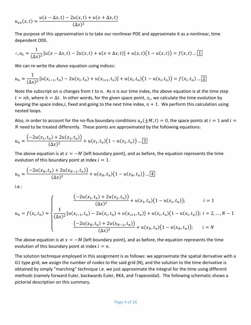
The solution technique employed in this assignment is as follows: we approximate the spatial derivative with a
G1 type grid, we assign the number of nodes to the said grid (N), and the solution to the time derivative is
obtained by simply “marching” technique i.e. we just approximate the integral for the time using different
methods (namely forward Euler, backwards Euler, RK4, and Trapezoidal). The following schematic shows a
pictorial description on this summary.
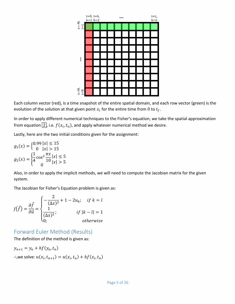
Page 5 of 26
Each column vector (red), is a time snapshot of the entire spatial domain, and each row vector (green) is the
evolution of the solution at that given point 𝑥𝑖 for the entire time from 0 to 𝑡𝑓.
In order to apply different numerical techniques to the Fisher’s equation, we take the spatial approximation
from equation 2 , i.e. 𝑓(𝑥𝑖, 𝑡𝑛), and apply whatever numerical method we desire.
Lastly, here are the two initial conditions given for the assignment:
𝑔1(𝑥) = {0.990
|𝑥| ≤ 15|𝑥| > 15
𝑔2(𝑥) = {1
4cos2
𝜋𝑥
100
|𝑥| ≤ 5|𝑥| > 5
Also, in order to apply the implicit methods, we will need to compute the Jacobian matrix for the given
system.
The Jacobian for Fisher’s Equation problem is given as:
𝐽(𝑓) =𝜕𝑓
𝜕�⃗⃗�=
{
−
2
(Δ𝑥)2+ 1 − 2𝑢𝑘; 𝑖𝑓 𝑘 = 𝑙
1
(Δ𝑥)2; 𝑖𝑓 |𝑘 − 𝑙| = 1
0; 𝑜𝑡ℎ𝑒𝑟𝑤𝑖𝑠𝑒
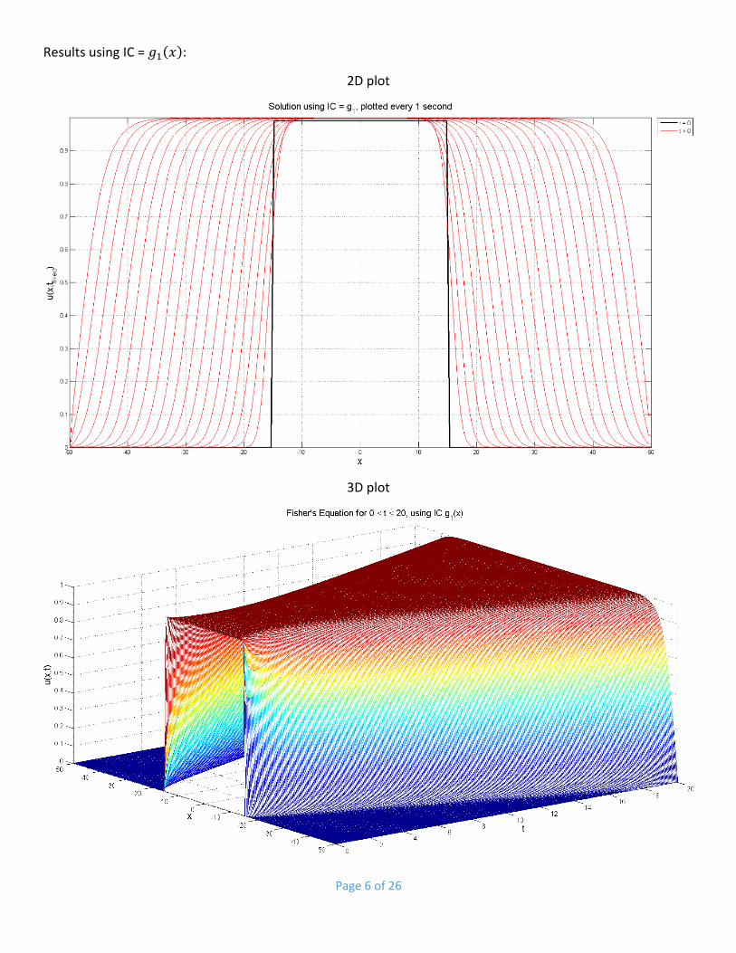
Forward Euler Method (Results)
The definition of the method is given as:
𝑦𝑛+1 = 𝑦𝑛 + ℎ𝑓(𝑦𝑛, 𝑡𝑛)
∴,we solve: 𝑢(𝑥𝑖, 𝑡𝑛+1) = 𝑢(𝑥𝑖, 𝑡𝑛) + ℎ𝑓(𝑥𝑖, 𝑡𝑛)
Page 6 of 26
Results using IC = 𝑔1(𝑥):
2D plot
3D plot
Page 7 of 26
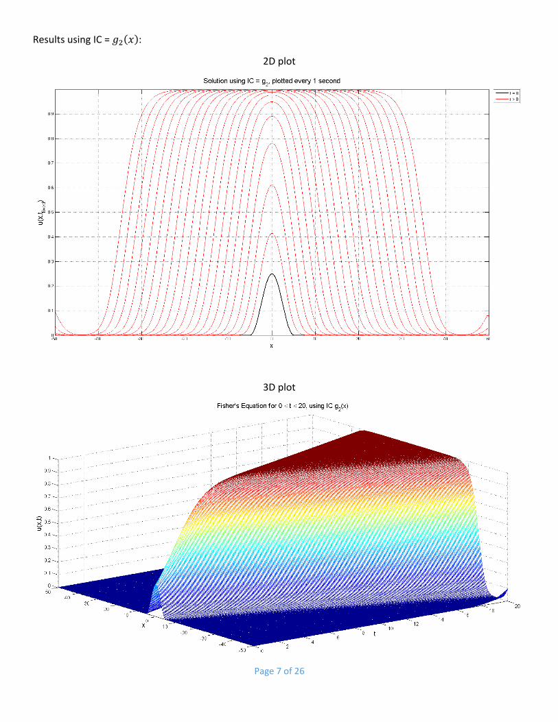
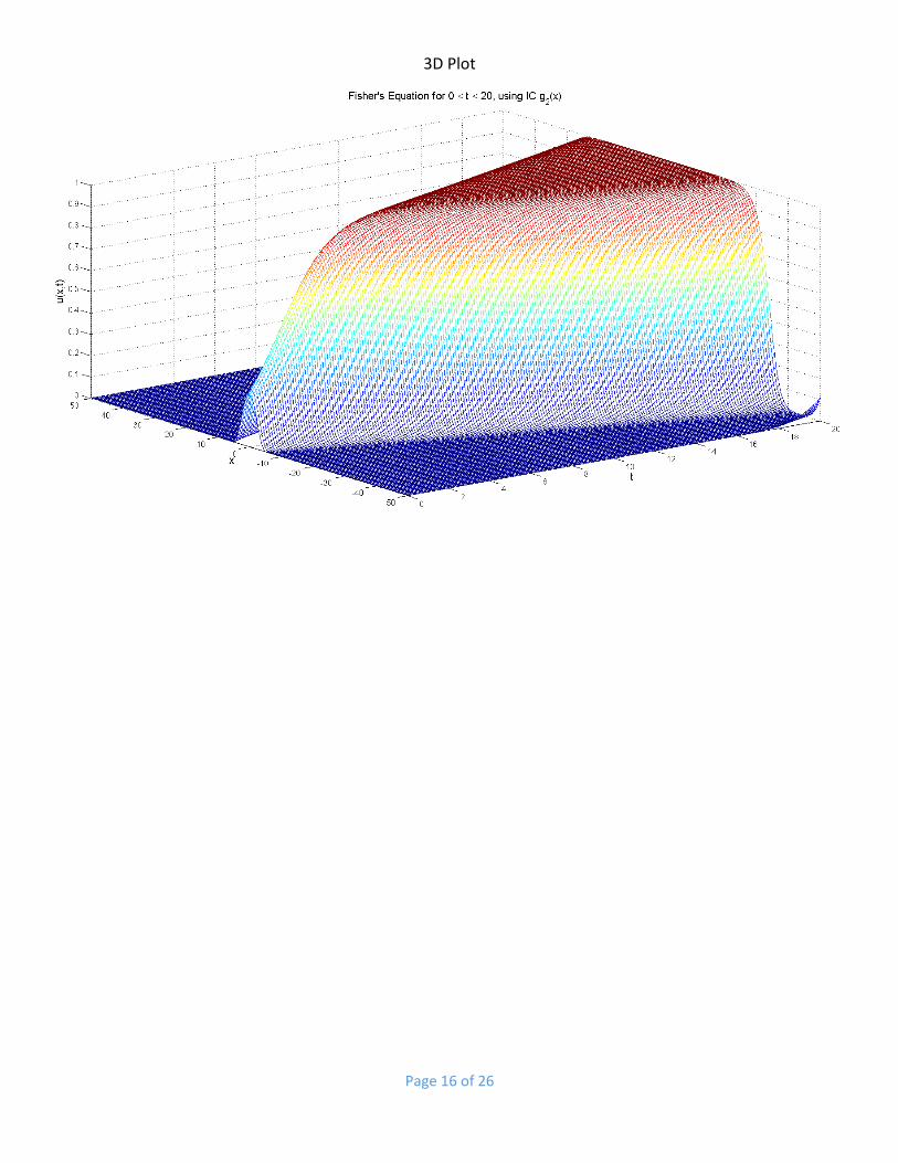
Results using IC = 𝑔2(𝑥):
2D plot
3D plot
Page 8 of 26
Runge-Kutta Method, 4th Order (Results)
The definition of the method is given as:
𝑢𝑛+1 = 𝑢𝑛 +ℎ
6(𝑘1 + 2𝑘2 + 2𝑘3 + 𝑘4)
𝑘1 = 𝑓(𝑡𝑛, 𝑢𝑛)
𝑘2 = 𝑓 (𝑡𝑛 +ℎ
2, 𝑢𝑛 +
ℎ𝑘12)
𝑘3 = 𝑓 (𝑡𝑛 +ℎ
2, 𝑢𝑛 +
ℎ𝑘22)
𝑘4 = 𝑓(𝑡𝑛 + ℎ, 𝑢𝑛 + ℎ𝑘3)
As our discretized system is “time independent”, the 𝑘 values simply become:
𝑘1 = 𝑓(𝑢𝑛) = 𝑢𝑛
𝑘2 = 𝑓 (𝑢𝑛 +ℎ𝑘12) = 𝑢𝑛 +
ℎ𝑘12
𝑘3 = 𝑓 (𝑢𝑛 +ℎ𝑘22) = 𝑢𝑛 +
ℎ𝑘22
𝑘4 = 𝑓(𝑢𝑛 + ℎ𝑘3) = 𝑢𝑛 + ℎ𝑘3
And since:
𝑢𝑛 = 𝑓(𝑥𝑖, 𝑡𝑛) ≈
{
(−2𝑢(𝑥1, 𝑡𝑛) + 2𝑢(𝑥2, 𝑡𝑛))
(Δ𝑥)2+ 𝑢(𝑥1, 𝑡𝑛)(1 − 𝑢(𝑥1, 𝑡𝑛)); 𝑖 = 1
1
(Δ𝑥)2[𝑢(𝑥𝑖−1, 𝑡𝑛) − 2𝑢(𝑥𝑖 , 𝑡𝑛) + 𝑢(𝑥𝑖+1, 𝑡𝑛)] + 𝑢(𝑥𝑖 , 𝑡𝑛)(1 − 𝑢(𝑥𝑖, 𝑡𝑛)); 𝑖 = 2,… ,𝑁 − 1
(−2𝑢(𝑥𝑁 , 𝑡𝑛) + 2𝑢(𝑥𝑁−1, 𝑡𝑛))
(Δ𝑥)2+ 𝑢(𝑥𝑁 , 𝑡𝑛)(1 − 𝑢(𝑥𝑁 , 𝑡𝑛)); 𝑖 = 𝑁
We are numerically solving the following system: 𝑢(𝑥𝑖, 𝑡𝑛+1 ) = 𝑢(𝑥𝑖, 𝑡𝑛) +ℎ
6(𝑘1 + 2𝑘2 + 2𝑘3 + 𝑘4)

Page 9 of 26
Results using IC = 𝑔1(𝑥):
2D plot
3D plot
Page 10 of 26
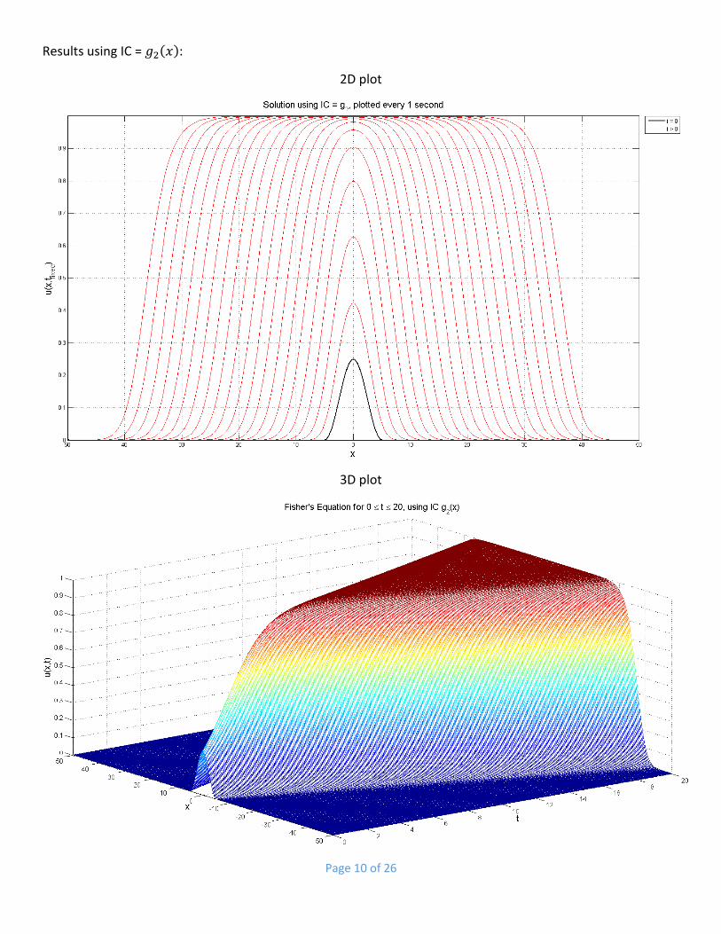
Results using IC = 𝑔2(𝑥):
2D plot
3D plot
Page 11 of 26
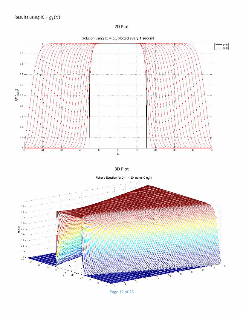
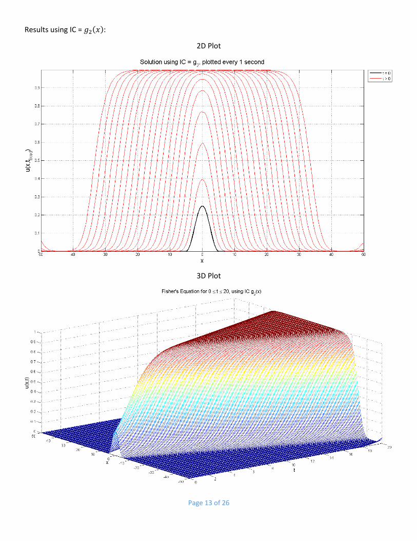
Trapezoidal Method (Results) The definition of the method is given as:
𝑦𝑛+1 = 𝑦𝑛 +1
2ℎ[𝑓(𝑦𝑛, 𝑡𝑛) + 𝑓(𝑦𝑛+1, 𝑡𝑛+1)]
However, since we have a nonlinear system, we need to solve for 𝑢𝑛+1 using Newton’s Method. For the n-
dimensional case, the Newton’s Method is given as:
�̃�𝑛+1 = 𝑢𝑛 − 𝐽−1(𝑓(𝑢𝑛))𝑓(𝑢𝑛)
The Jacobian is defined as:
𝐽(𝑓) =𝜕𝑓
𝜕�⃗⃗�=
{
−
2
(Δ𝑥)2+ 1 − 2𝑢𝑘; 𝑖𝑓 𝑘 = 𝑙
1
(Δ𝑥)2; 𝑖𝑓 |𝑘 − 𝑙| = 1
0; 𝑜𝑡ℎ𝑒𝑟𝑤𝑖𝑠𝑒
The computational challenge with such an approach is that we cannot choose ℎ and Δ𝑥 with the same degree
of freedom as we were allowed in the explicit methods. This is due to the fact that the Jacobian matrix must
be a square matrix in order for the inverse to exist. Therefore, the grid size for both 𝑡 and 𝑥 has to be the
same.
The following results were obtained, using Newton’s method with a tolerance of 10−4. The general shape of
the result matches that of the two explicit methods discussed above.
The approximation, �̃�𝑛+1, obtained from Newton’s Method is implemented in the following manner:
𝑢𝑛+1 = 𝑢𝑛 +1
2ℎ[𝑢𝑛 + �̃�𝑛+1]
Page 12 of 26
Results using IC = 𝑔1(𝑥):
2D Plot
3D Plot
Page 13 of 26
Results using IC = 𝑔2(𝑥):
2D Plot
3D Plot
Page 14 of 26
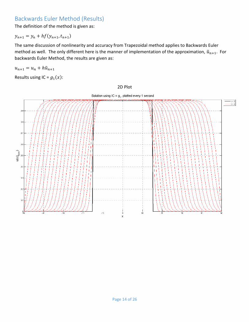
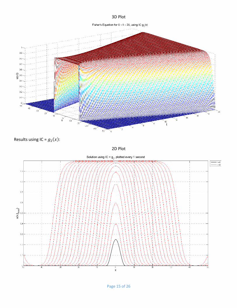
Backwards Euler Method (Results) The definition of the method is given as:
𝑦𝑛+1 = 𝑦𝑛 + ℎ𝑓(𝑦𝑛+1, 𝑡𝑛+1)
The same discussion of nonlinearity and accuracy from Trapezoidal method applies to Backwards Euler
method as well. The only different here is the manner of implementation of the approximation, �̃�𝑛+1. For
backwards Euler Method, the results are given as:
𝑢𝑛+1 = 𝑢𝑛 + ℎ�̃�𝑛+1
Results using IC = 𝑔1(𝑥):
2D Plot
Page 15 of 26
3D Plot
Results using IC = 𝑔2(𝑥):
2D Plot
Page 16 of 26
3D Plot
Page 17 of 26
Forward Euler Method (MATLAB Code) %Code for Forward Euler Method
clear
clc
%Initializing constants, parameters, and data structures
N = 200; %Number of space points
M = 50; %Space endpoint
t0 = 0; %Initial time
tf = 20; %Final time
h = (tf-t0)/(N-1); %Delta t
t = t0:h:tf; %Time vector
dx = (2*M)/(N-1); %Delta x
x = -M:dx:M; %Space vector
g1 = zeros(length(x),1); %IC 1 Vector
g2 = zeros(length(x),1); %IC 2 Vector
u = zeros(N,length(t)); %Solution Matrix
%Create IC g1
for i = 1:N
if abs(x(i))<= 15
g1(i,1) = 0.99;
end
end
%Create IC g2
for i = 1:N
if abs(x(i))<= 5
g2(i,1) = 0.25*(cos((pi*x(i))/10))^2;
end
end
%---------------Solving using Forward Euler and IC 1----------------------%
u(:,1) = g1(:,1);
%i = 1
for n = 1:length(t)-1
fn = (1/dx^2)*(-2*u(1,n) + 2*u(2,n))+u(1,n)*(1-u(1,n));
u(1,n+1)=u(1,n)+h*(fn);
end
%i = 2,3,...,N-1
for n = 1:length(t)-1
fn = (1/dx^2).*(u(1:N-2,n)-2.*u(2:N-1,n)+u(3:N,n))+u(2:N-1,n).*(1-u(2:N-1,n));
u(2:N-1,n+1)=u(2:N-1,n)+h*(fn);
end
%i = N
for n = 1:length(t)-1
fn = (1/dx^2)*(2*u(N-1,n)-2*u(N,n))+u(N,n)*(1-u(N,n));
u(N,n+1)=u(N,n)+h*(fn);
end
%Plot solutions using IC g1
figure1 = figure;
plot(x,u(:,1),'black','linewidth',2)
hold on
%This part produces profile for each second starting at 1 to 20
for i = 2:length(t)
if rem(t(i),1) == 0
plot(x,u(:,i),'r')
end
end
legend('t = 0','t > 0','location','northeastoutside')
title('Solution using IC = g_1, plotted every 1 second','fontsize',16)
xlabel('x','fontsize',16)
Page 18 of 26
ylabel('u(x,t_{fixed})','fontsize',16)
grid on
axis tight
hold off
%------------Solving using Forward Euler and IC 2-------------------------%
u(:,1) = g2(:,1);
%i = 1
for n = 1:length(t)-1
fn = (1/dx^2)*(-2*u(1,n) + 2*u(2,n))+u(1,n)*(1-u(1,n));
u(1,n+1)=u(1,n)+h*(fn);
end
%i = 2,3,...,N-1
for n = 1:length(t)-1
fn = (1/dx^2).*(u(1:N-2,n)-2.*u(2:N-1,n)+u(3:N,n))+u(2:N-1,n).*(1-u(2:N-1,n));
u(2:N-1,n+1)=u(2:N-1,n)+h*(fn);
end
%i = N
for n = 1:length(t)-1
fn = (1/dx^2)*(2*u(N-1,n)-2*u(N,n))+u(N,n)*(1-u(N,n));
u(N,n+1)=u(N,n)+h*(fn);
end
%Plot solutions using IC g2
figure2 = figure;
plot(x,u(:,1),'black','linewidth',2)
hold on
%This part produces profile for each second starting at 1 to 20
for i = 2:length(t)
if rem(t(i),1) == 0
plot(x,u(:,i),'r')
end
end
legend('t = 0','t > 0','location','northeastoutside')
title('Solution using IC = g_2, plotted every 1 second','fontsize',16)
xlabel('x','fontsize',16)
ylabel('u(x,t_{fixed})','fontsize',16)
grid on
axis tight
hold off
Runge-Kutta Method, 4th Order (MATLAB Code) %Code for RK4 Method
clear
clc
%Initializing constants, parameters, and data structures
N = 200; %Number of space points
M = 50; %Space endpoint
t0 = 0; %Initial time
tf = 20; %Final time
h = (tf-t0)/(N-1); %Delta t
t = t0:h:tf; %Time vector
dx = (2*M)/(N-1); %Delta x
x = -M:dx:M; %Space vector
g1 = zeros(length(x),1); %IC 1 Vector
g2 = zeros(length(x),1); %IC 2 Vector
u = zeros(N,length(t)); %Solution Matrix
%Create IC g1
for i = 1:N
if abs(x(i))<= 15
Page 19 of 26
g1(i,1) = 0.99;
end
end
%Create IC g2
for i = 1:N
if abs(x(i))<= 5
g2(i,1) = 0.25*(cos((pi*x(i))/10))^2;
end
end
%----------------------Solving using RK4 and IC 2-------------------------%
u(:,1) = g1(:,1);
%i = 1
for n = 1:length(t)-1
k1 = (1/dx^2)*(-2*u(1,n) + 2*u(2,n)) + u(1,n)*(1-u(1,n));
k2 = k1 + 0.5*h.*k1;
k3 = k2 + 0.5*h.*k2;
k4 = k3 + h.*k3;
u(1,n+1)=u(1,n) + h/6*(k1 + 2.*k2 + 2.*k3 + k4);
end
%i = 2,3,...,N-1
for n = 1:length(t)-1
for i = 2:N-1
k1 = (1/dx^2)*(u(i-1,n)-2*u(i,n)+u(i+1,n)) + u(i,n)*(1-u(i,n));
k2 = k1 + 0.5*h.*k1;
k3 = k2 + 0.5*h.*k2;
k4 = k3 + h.*k3;
u(i,n+1)=u(i,n) + h/6*(k1 + 2.*k2 + 2.*k3 + k4);
end
end
%i = N
for n = 1:length(t)-1
k1 = (1/dx^2)*(2*u(N-1,n)-2*u(N,n)) + u(N,n)*(1-u(N,n));
k2 = k1 + 0.5*h.*k1;
k3 = k2 + 0.5*h.*k2;
k4 = k3 + h.*k3;
u(N,n+1)=u(N,n) + h/6*(k1 + 2.*k2 + 2.*k3 + k4);
end
%Plot solutions using IC g1
figure1 = figure;
plot(x,u(:,1),'black','linewidth',2)
hold on
%This part produces profile for each second starting at 1 to 20
for i = 2:length(t)
if rem(t(i),1) == 0
plot(x,u(:,i),'r')
end
end
legend('t = 0','t > 0','location','northeastoutside')
title('Solution using IC = g_1, plotted every 1 second','fontsize',16)
xlabel('x','fontsize',16)
ylabel('u(x,t_{fixed})','fontsize',16)
grid on
axis tight
hold off
k1 = 0; k2 = 0; k3 = 0; k4 = 0;
u = zeros(N,length(t));
%----------------------Solving using RK4 and IC 2-------------------------%
u(:,1) = g2(:,1);
Page 20 of 26
%i = 1
for n = 1:length(t)-1
k1 = (1/dx^2)*(-2*u(1,n) + 2*u(2,n)) + u(1,n)*(1-u(1,n));
k2 = k1 + 0.5*h.*k1;
k3 = k2 + 0.5*h.*k2;
k4 = k3 + h.*k3;
u(1,n+1)=u(1,n) + h/6*(k1 + 2.*k2 + 2.*k3 + k4);
end
%i = 2,3,...,N-1
for n = 1:length(t)-1
for i = 2:N-1
k1 = (1/dx^2)*(u(i-1,n)-2*u(i,n)+u(i+1,n)) + u(i,n)*(1-u(i,n));
k2 = k1 + 0.5*h.*k1;
k3 = k2 + 0.5*h.*k2;
k4 = k3 + h.*k3;
u(i,n+1)=u(i,n) + h/6*(k1 + 2.*k2 + 2.*k3 + k4);
end
end
%i = N
for n = 1:length(t)-1
k1 = (1/dx^2)*(2*u(N-1,n)-2*u(N,n)) + u(N,n)*(1-u(N,n));
k2 = k1 + 0.5*h.*k1;
k3 = k2 + 0.5*h.*k2;
k4 = k3 + h.*k3;
u(N,n+1)=u(N,n) + h/6*(k1 + 2.*k2 + 2.*k3 + k4);
end
%Plot solutions using IC g2
figure2 = figure;
plot(x,u(:,1),'black','linewidth',2)
hold on
%This part produces profile for each second starting at 1 to 20
for i = 2:length(t)
if rem(t(i),1) == 0
plot(x,u(:,i),'r')
end
end
legend('t = 0','t > 0','location','northeastoutside')
title('Solution using IC = g_2, plotted every 1 second','fontsize',16)
xlabel('x','fontsize',16)
ylabel('u(x,t_{fixed})','fontsize',16)
grid on
axis tight
hold off
Trapezoidal Method (MATLAB Code) %Code for Trapezoidal Method clear clc
%Initializing constants, parameters, and data structures N = 200; %Number of space points M = 50; %Space endpoint t0 = 0; %Initial time tf = 20; %Final time tol = 10^-4; %Tolerance for Newton's Method h = (tf-t0)/(N-1); %Delta t t = t0:h:tf; %Time vector dx = (2*M)/(N-1); %Delta x x = -M:dx:M; %Space vector g1 = zeros(length(x),1); %IC 1 Vector g2 = zeros(length(x),1); %IC 2 Vector u = zeros(N,length(t)); %Solution Matrix J = zeros(N,length(t)); %Jacobian Matrix
Page 21 of 26
u1 = 0; u2 = 0;
%Create IC g1 for i = 1:N if abs(x(i))<= 15 g1(i,1) = 0.99; end end
%Create IC g2 for i = 1:N if abs(x(i))<= 5 g2(i,1) = 0.25*(cos((pi*x(i))/10))^2; end end
%-----------------Solving using Trapaziodal and IC 1----------------------% u(:,1) = g1(:,1);
%Deriving the Jacobian for n1 = 1:N for k1 = 1:length(t) if n1 == k1 J(n1,k1) = 1/dx^2 + 1 - 2*u(n1,k1); else if abs(k1 - n1) == 1 J(n1,k1) = 1/dx^2; else J(n1,k1) = 0; end end end end
Ji = inv(J);
%i = 1 for n = 1:length(t)-1 fn = (1/dx^2)*(-2*u(1,n) + 2*u(2,n))+u(1,n)*(1-u(1,n)); u1 = fn; while(abs(norm(u1)-norm(u2))) >= tol u2 = u1 - Ji(2,n+1)*fn; u1 = u2; end u(1,n+1)=u(1,n)+(h/2)*(fn + u1); end
%i = 2,3,...,N-1 for n = 1:length(t)-1 fn = (1/dx^2).*(u(1:N-2,n)-2.*u(2:N-1,n)+u(3:N,n))+u(2:N-1,n).*(1-u(2:N-1,n)); u1 = fn; while(abs(norm(u1)-norm(u2))) >= tol u2 = u1 - Ji(3:N,n+1).*fn; u1 = u2; end u(2:N-1,n+1)=u(2:N-1,n)+(h/2)*(fn + u1); end
%i = N for n = 1:length(t)-1 fn = (1/dx^2)*(2*u(N-1,n)-2*u(N,n))+u(N,n)*(1-u(N,n)); u1 = fn; while(abs(norm(u1)-norm(u2))) >= tol u2 = u1 - Ji(N,n+1)*fn; u1 = u2; end u(N,n+1)=u(N,n)+(h/2)*(fn + u1);
Page 22 of 26
end
%Plot solutions using IC g1 figure1 = figure; plot(x,u(:,1),'black','linewidth',2) hold on %This part produces profile for each second starting at 1 to 20 for i = 2:length(t) if rem(i,10) == 0 plot(x,u(:,i),'r') end end legend('t = 0','t > 0','location','northeastoutside') title('Solution using IC = g_1, plotted every 1 second','fontsize',16) xlabel('x','fontsize',16) ylabel('u(x,t_{fixed})','fontsize',16) grid on axis tight hold off
%-----------------Solving using Trapezoidal and IC 2----------------------% u(:,1) = g2(:,1);
%Deriving the Jacobian for n1 = 1:N for k1 = 1:length(t) if n1 == k1 J(n1,k1) = 1/dx^2 + 1 - 2*u(n1,k1); else if abs(k1 - n1) == 1 J(n1,k1) = 1/dx^2; else J(n1,k1) = 0; end end end end
Ji = inv(J);
%i = 1 for n = 1:length(t)-1 fn = (1/dx^2)*(-2*u(1,n) + 2*u(2,n))+u(1,n)*(1-u(1,n)); u1 = fn; while(abs(norm(u1)-norm(u2))) >= tol u2 = u1 - Ji(1,n+1)*fn; u1 = u2; end u(1,n+1)=u(1,n)+(h/2)*(fn + u1); end
%i = 2,3,...,N-1 for n = 1:length(t)-1 fn = (1/dx^2).*(u(1:N-2,n)-2.*u(2:N-1,n)+u(3:N,n))+u(2:N-1,n).*(1-u(2:N-1,n)); u1 = fn; while(abs(norm(u1)-norm(u2))) >= tol u2 = u1 - Ji(2:N-1,n+1).*fn; u1 = u2; end u(2:N-1,n+1)=u(2:N-1,n)+(h/2)*(fn + u1); end
%i = N for n = 1:length(t)-1 fn = (1/dx^2)*(2*u(N-1,n)-2*u(N,n))+u(N,n)*(1-u(N,n)); u1 = fn;
Page 23 of 26
while(abs(norm(u1)-norm(u2))) >= tol u2 = u1 - Ji(1,n+1)*fn; u1 = u2; end u(N,n+1)=u(N,n)+(h/2)*(fn + u1); end
%Plot solutions using IC g2 figure1 = figure; plot(x,u(:,1),'black','linewidth',2) hold on %This part produces profile for each second starting at 1 to 20 for i = 2:length(t) if rem(i,10) == 0 plot(x,u(:,i),'r') end end legend('t = 0','t > 0','location','northeastoutside') title('Solution using IC = g_2, plotted every 1 second','fontsize',16) xlabel('x','fontsize',16) ylabel('u(x,t_{fixed})','fontsize',16) grid on axis tight hold off
Backwards Euler Method (MATLAB Code) %Code for Backwards Euler Method clear clc
%Initializing constants, parameters, and data structures N = 200; %Number of space points M = 50; %Space endpoint t0 = 0; %Initial time tf = 20; %Final time tol = 10^-4; %Tolerance for Newton's Method h = (tf-t0)/(N-1); %Delta t t = t0:h:tf; %Time vector dx = (2*M)/(N-1); %Delta x x = -M:dx:M; %Space vector g1 = zeros(length(x),1); %IC 1 Vector g2 = zeros(length(x),1); %IC 2 Vector u = zeros(N,length(t)); %Solution Matrix J = zeros(N,length(t)); %Jacobian Matrix u1 = 0; u2 = 0;
%Create IC g1 for i = 1:N if abs(x(i))<= 15 g1(i,1) = 0.99; end end
%Create IC g2 for i = 1:N if abs(x(i))<= 5 g2(i,1) = 0.25*(cos((pi*x(i))/10))^2; end end
%------------Solving using backward Euler and IC 1------------------------% u(:,1) = g1(:,1);
%Deriving the Jacobian for n1 = 1:N
Page 24 of 26
for k1 = 1:length(t) if n1 == k1 J(n1,k1) = 1/dx^2 + 1 - 2*u(n1,k1); else if abs(k1 - n1) == 1 J(n1,k1) = 1/dx^2; else J(n1,k1) = 0; end end end end
Ji = inv(J);
%i = 1 for n = 1:length(t)-1 fn = (1/dx^2)*(-2*u(1,n) + 2*u(2,n))+u(1,n)*(1-u(1,n)); u1 = fn; while(abs(norm(u1)-norm(u2))) >= tol u2 = u1 - Ji(2,n+1)*fn; u1 = u2; end u(1,n+1)=u(1,n)+(h)*(u1); end
%i = 2,3,...,N-1 for n = 1:length(t)-1 fn = (1/dx^2).*(u(1:N-2,n)-2.*u(2:N-1,n)+u(3:N,n))+u(2:N-1,n).*(1-u(2:N-1,n)); u1 = fn; while(abs(norm(u1)-norm(u2))) >= tol u2 = u1 - Ji(3:N,n+1).*fn; u1 = u2; end u(2:N-1,n+1)=u(2:N-1,n)+(h)*(u1); end
%i = N for n = 1:length(t)-1 fn = (1/dx^2)*(2*u(N-1,n)-2*u(N,n))+u(N,n)*(1-u(N,n)); u1 = fn; while(abs(norm(u1)-norm(u2))) >= tol u2 = u1 - Ji(N,n+1)*fn; u1 = u2; end u(N,n+1)=u(N,n)+(h)*(u1); end
%Plot solutions using IC g1 figure1 = figure; plot(x,u(:,1),'black','linewidth',2) hold on %This part produces profile for each second starting at 1 to 20 for i = 2:length(t) if rem(i,10) == 0 plot(x,u(:,i),'r') end end legend('t = 0','t > 0','location','northeastoutside') title('Solution using IC = g_1, plotted every 1 second','fontsize',16) xlabel('x','fontsize',16) ylabel('u(x,t_{fixed})','fontsize',16) grid on axis tight hold off
Page 25 of 26
%------------Solving using backward Euler and IC 2------------------------% u(:,1) = g2(:,1);
%Deriving the Jacobian for n1 = 1:N for k1 = 1:length(t) if n1 == k1 J(n1,k1) = 1/dx^2 + 1 - 2*u(n1,k1); else if abs(k1 - n1) == 1 J(n1,k1) = 1/dx^2; else J(n1,k1) = 0; end end end end
Ji = inv(J);
%i = 1 for n = 1:length(t)-1 fn = (1/dx^2)*(-2*u(1,n) + 2*u(2,n))+u(1,n)*(1-u(1,n)); u1 = fn; while(abs(norm(u1)-norm(u2))) >= tol u2 = u1 - Ji(1,n+1)*fn; u1 = u2; end u(1,n+1)=u(1,n)+(h)*(u1); end
%i = 2,3,...,N-1 for n = 1:length(t)-1 fn = (1/dx^2).*(u(1:N-2,n)-2.*u(2:N-1,n)+u(3:N,n))+u(2:N-1,n).*(1-u(2:N-1,n)); u1 = fn; while(abs(norm(u1)-norm(u2))) >= tol u2 = u1 - Ji(2:N-1,n+1).*fn; u1 = u2; end u(2:N-1,n+1)=u(2:N-1,n)+(h)*(u1); end
%i = N for n = 1:length(t)-1 fn = (1/dx^2)*(2*u(N-1,n)-2*u(N,n))+u(N,n)*(1-u(N,n)); u1 = fn; while(abs(norm(u1)-norm(u2))) >= tol u2 = u1 - Ji(1,n+1)*fn; u1 = u2; end u(N,n+1)=u(N,n)+(h)*(u1); end
%Plot solutions using IC g2 figure1 = figure; plot(x,u(:,1),'black','linewidth',2) hold on %This part produces profile for each second starting at 1 to 20 for i = 2:length(t) if rem(i,10) == 0 plot(x,u(:,i),'r') end end legend('t = 0','t > 0','location','northeastoutside') title('Solution using IC = g_2, plotted every 1 second','fontsize',16) xlabel('x','fontsize',16) ylabel('u(x,t_{fixed})','fontsize',16)
Page 26 of 26
grid on axis tight hold off
References
Salsa, Sandro. Partial Differential Equations in Action: From Modelling to Theory. 1st ed. Milan: Springer, 2008.
Debnath, Lokenath. Nonlinear Partial Differential Equations for Scientists and Engineers. 3rd ed. New York,
2012.