PARTIAL DIFFERENTIAL EQUATIONS

I Introduction

An equation containing partial derivatives of a function of two or more independent

variables is called a partial differential equation (PDE).

e.g. y2∂u

∂x+

∂u

∂y= u where u(x, y) is the unknown function.

For convenience we denote

ux =∂u

∂x, uxx =

∂2u

∂x2, uxy =

∂2u

∂x∂y, etc.

so that the above PDE can be written y2ux + uy = u. The order of the PDE is the

order of the highest partial derivative. A PDE whose unknown function and its

partial derivatives appear linearly in the equation is said to be linear. For example,

A(x, y)uxx +B(x, y)uxy + C(x, y)uyy +D(x, y)ux +E(x, y)uy + F (x, y)u = G(x, y)

which is the general form of second-order linear PDE. If each term in the PDE contains

either the dependent variable or one of its derivatives, i.e., G(x, y) = 0, then it is said

to be homogeneous, otherwise it is nonhomogeneous.

2

Examples

1. ut = c2uxx 1 dimensional heat conduction equation

2. utt = c2uxx 1 dimensional wave equation

3. uxx + uyy = 0 2 dimensional Laplace equation

4. uxx + uyy = f(x, y) 2 dimensional Poisson equation

5. uxx + uyy =1

c2utt − λ2u 2 dimensional Klein-Gordon equation

6. utt = c2(uxx + uyy + uzz) 3 dimensional wave equation

In general, the solution of PDE presents a much more difficult problem than

the solution of ODE and except for certain special types of linear PDE, no general

method of solution is available. It is remarkable and fortunate that a large number

of the important equations in practice are not only linear, but also of second order,

for which solutions are relatively easy to find.

A solution of a PDE in some region R of the space of the independent variables

is a function that has all the partial derivatives appearing in the equation in some

domain containing R, and satisfies the equation everywhere in R.

In general, the totality of solutions of a PDE is very large.

Example. The functions

(i) u = x3 − 3xy2 (ii) u = sinx cosh y

(iii) u = ln(x2 + y2) (iv) u = tan−1³yx

´are all solutions of the 2 dimensional Laplace equation uxx + uyy = 0, altough they

are entirely different from each other.

The Heat Equation (Diffusion equation) 3

Theorem

(i) If u1 and u2 are two solutions of a linear homogeneous PDE in some region,

then u = k1u1+ k2u2 is also a solution of the PDE in that region, where k1 and

k2 are constants.

(ii) u ≡ 0 is always a solution of a linear homogeneous PDE.

Proof Trivial.

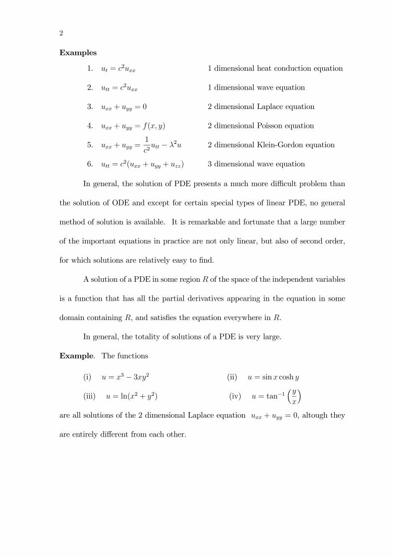
II The Heat Equation (Diffusion equation)

Consider a thin metal rod with cross-section area A. Assume that the lateral surface

is wrapped with insulation such that heat conducts along the x-direction only.

x 0x

L

x∆

Figure 1

Let u(x, t) denote the temperature at position x, at time t.

Newton’s law of cooling (Fourier’s law) =⇒ the quantity of heat (flux) flowing across

x0 per unit time is proportional to the temperature gradient at x0.

Therefore Qx0 = −kAux(x0, t) where k is the thermal conductivity of the metal.

The quantity of heat loss along a small segment [x0, x0 +4x] per unit time is given

byH = Qx0 −Qx0+4x = kA [ux(x0 +4x, t)− ux(x0, t)] .

4

The average change in temperature 4u in the time interval 4t is proportional to the

amount of heat loss and inversely proportional to the mass 4m of the element.

Therefore 4u =H4t

s4m, where s is the specific heat of the metal. This gives

4u

4t=

kA [ux(x0 +4x, t)− ux(x0, t)]

sρA4x

=k

sρ

[ux(x0 +4x, t)− ux(x0, t)]

4x−→ k

sρuxx(x0, t) as 4x→ 0.

On the other hand, 4x→ 0 =⇒ 4t→ 0 =⇒ 4u

4t→ ut(x0, t), therefore

ut(x, t) =k

sρuxx(x0, t) =⇒ ut = c2uxx

where c2 =k

sρis called the thermal diffusivity of the material (note that k, s, ρ are

all properties of the material and are all positive).

Note If heat is added or removed from the rod, then the equation becomes ut =

c2uxx+f(x, t) which is nonhomogeneous and f(x, t) is the heat source or sink density.

Suppose that the ends x = 0 and x = L of the rod are kept at temperatures T0 and

T1, and the initial temperature distribution of the rod is f(x), then the boundary

conditions (B.C.) are u(0, t) = T0 and u(L, t) = T1, while the initial condition (I.C.)

is u(x, 0) = f(x).

The problem becomes an initial boundary value problem (IBVP):

ut = c2uxx; 0 < x < L, 0 < t <∞,

B.C.

u(0, t) = T0,

u(L, t) = T1,

0 < t <∞,

I.C. u(x, 0) = f(x), 0 < x < L.

The Heat Equation (Diffusion equation) 5

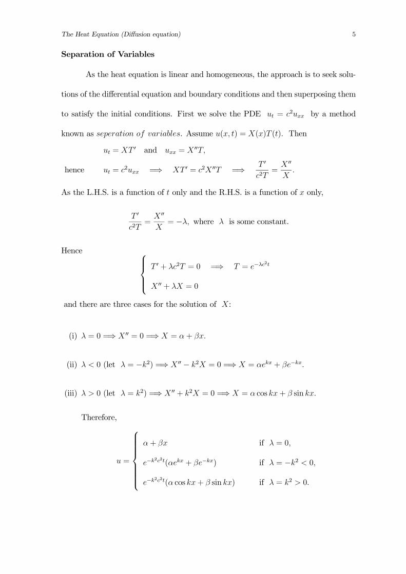
Separation of Variables

As the heat equation is linear and homogeneous, the approach is to seek solu-

tions of the differential equation and boundary conditions and then superposing them

to satisfy the initial conditions. First we solve the PDE ut = c2uxx by a method

known as seperation of variables. Assume u(x, t) = X(x)T (t). Then

ut = XT 0 and uxx = X 00T,

hence ut = c2uxx =⇒ XT 0 = c2X 00T =⇒ T 0

c2T=

X 00

X.

As the L.H.S. is a function of t only and the R.H.S. is a function of x only,

T 0

c2T=

X 00

X= −λ, where λ is some constant.

Hence T 0 + λc2T = 0 =⇒ T = e−λc

2t

X 00 + λX = 0

and there are three cases for the solution of X:

(i) λ = 0 =⇒ X 00 = 0 =⇒ X = α+ βx.

(ii) λ < 0 (let λ = −k2) =⇒ X 00 − k2X = 0 =⇒ X = αekx + βe−kx.

(iii) λ > 0 (let λ = k2) =⇒ X 00 + k2X = 0 =⇒ X = α cos kx+ β sin kx.

Therefore,

u =

α+ βx if λ = 0,

e−k2c2t(αekx + βe−kx) if λ = −k2 < 0,

e−k2c2t(α cos kx+ β sin kx) if λ = k2 > 0.

6

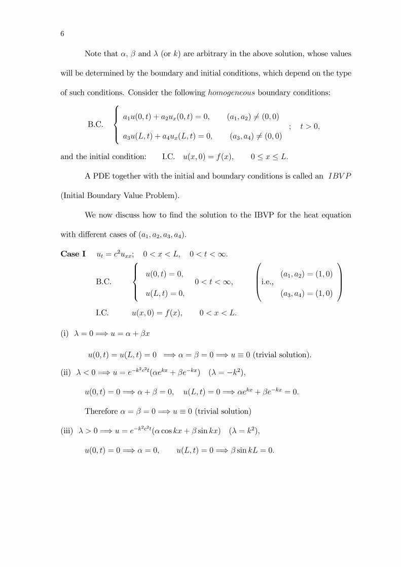
Note that α, β and λ (or k) are arbitrary in the above solution, whose values

will be determined by the boundary and initial conditions, which depend on the type

of such conditions. Consider the following homogeneous boundary conditions:

B.C.

a1u(0, t) + a2ux(0, t) = 0, (a1, a2) 6= (0, 0)

a3u(L, t) + a4ux(L, t) = 0, (a3, a4) 6= (0, 0); t > 0,

and the initial condition: I.C. u(x, 0) = f(x), 0 ≤ x ≤ L.

A PDE together with the initial and boundary conditions is called an IBV P

(Initial Boundary Value Problem).

We now discuss how to find the solution to the IBVP for the heat equation

with different cases of (a1, a2, a3, a4).

Case I ut = c2uxx; 0 < x < L, 0 < t <∞.

B.C.

u(0, t) = 0,

u(L, t) = 0,

0 < t <∞,

i.e., (a1, a2) = (1, 0)(a3, a4) = (1, 0)

I.C. u(x, 0) = f(x), 0 < x < L.

(i) λ = 0 =⇒ u = α+ βx

u(0, t) = u(L, t) = 0 =⇒ α = β = 0 =⇒ u ≡ 0 (trivial solution).(ii) λ < 0 =⇒ u = e−k

2c2t(αekx + βe−kx) (λ = −k2),

u(0, t) = 0 =⇒ α+ β = 0, u(L, t) = 0 =⇒ αekx + βe−kx = 0.

Therefore α = β = 0 =⇒ u ≡ 0 (trivial solution)

(iii) λ > 0 =⇒ u = e−k2c2t(α cos kx+ β sin kx) (λ = k2),

u(0, t) = 0 =⇒ α = 0, u(L, t) = 0 =⇒ β sin kL = 0.

The Heat Equation (Diffusion equation) 7

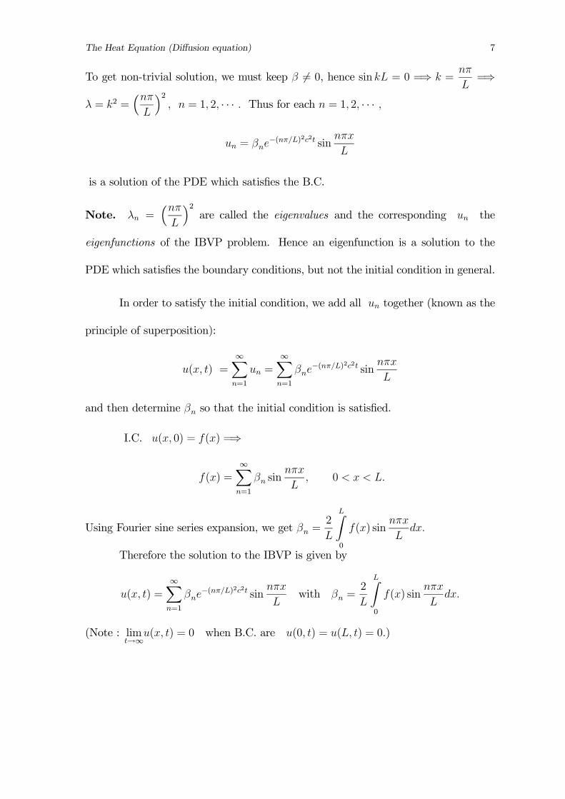
To get non-trivial solution, we must keep β 6= 0, hence sin kL = 0 =⇒ k =nπ

L=⇒

λ = k2 =³nπL

´2, n = 1, 2, · · · . Thus for each n = 1, 2, · · · ,

un = βne−(nπ/L)2c2t sin

nπx

L

is a solution of the PDE which satisfies the B.C.

Note. λn =³nπL

´2are called the eigenvalues and the corresponding un the

eigenfunctions of the IBVP problem. Hence an eigenfunction is a solution to the

PDE which satisfies the boundary conditions, but not the initial condition in general.

In order to satisfy the initial condition, we add all un together (known as the

principle of superposition):

u(x, t) =∞Xn=1

un =∞Xn=1

βne−(nπ/L)2c2t sin

nπx

L

and then determine βn so that the initial condition is satisfied.

I.C. u(x, 0) = f(x) =⇒

f(x) =∞Xn=1

βn sinnπx

L, 0 < x < L.

Using Fourier sine series expansion, we get βn =2

L

LZ0

f(x) sinnπx

Ldx.

Therefore the solution to the IBVP is given by

u(x, t) =∞Xn=1

βne−(nπ/L)2c2t sin

nπx

Lwith βn =

2

L

LZ0

f(x) sinnπx

Ldx.

(Note : limt→∞

u(x, t) = 0 when B.C. are u(0, t) = u(L, t) = 0.)

8

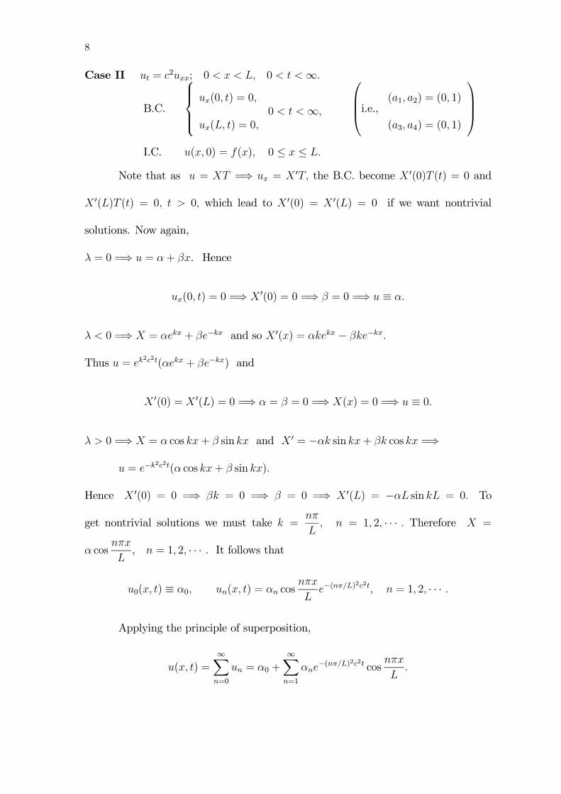
Case II ut = c2uxx; 0 < x < L, 0 < t <∞.

B.C.

ux(0, t) = 0,

ux(L, t) = 0,0 < t <∞,

i.e., (a1, a2) = (0, 1)(a3, a4) = (0, 1)

I.C. u(x, 0) = f(x), 0 ≤ x ≤ L.

Note that as u = XT =⇒ ux = X 0T, the B.C. become X 0(0)T (t) = 0 and

X 0(L)T (t) = 0, t > 0, which lead to X 0(0) = X 0(L) = 0 if we want nontrivial

solutions. Now again,

λ = 0 =⇒ u = α+ βx. Hence

ux(0, t) = 0 =⇒ X 0(0) = 0 =⇒ β = 0 =⇒ u ≡ α.

λ < 0 =⇒ X = αekx + βe−kx and so X 0(x) = αkekx − βke−kx.

Thus u = ek2c2t(αekx + βe−kx) and

X 0(0) = X 0(L) = 0 =⇒ α = β = 0 =⇒ X(x) = 0 =⇒ u ≡ 0.

λ > 0 =⇒ X = α cos kx+ β sin kx and X 0 = −αk sin kx+ βk cos kx =⇒

u = e−k2c2t(α cos kx+ β sin kx).

Hence X 0(0) = 0 =⇒ βk = 0 =⇒ β = 0 =⇒ X 0(L) = −αL sin kL = 0. To

get nontrivial solutions we must take k =nπ

L, n = 1, 2, · · · . Therefore X =

α cosnπx

L, n = 1, 2, · · · . It follows that

u0(x, t) ≡ α0, un(x, t) = αn cosnπx

Le−(nπ/L)

2c2t, n = 1, 2, · · · .

Applying the principle of superposition,

u(x, t) =∞Xn=0

un = α0 +∞Xn=1

αne−(nπ/L)2c2t cos

nπx

L.

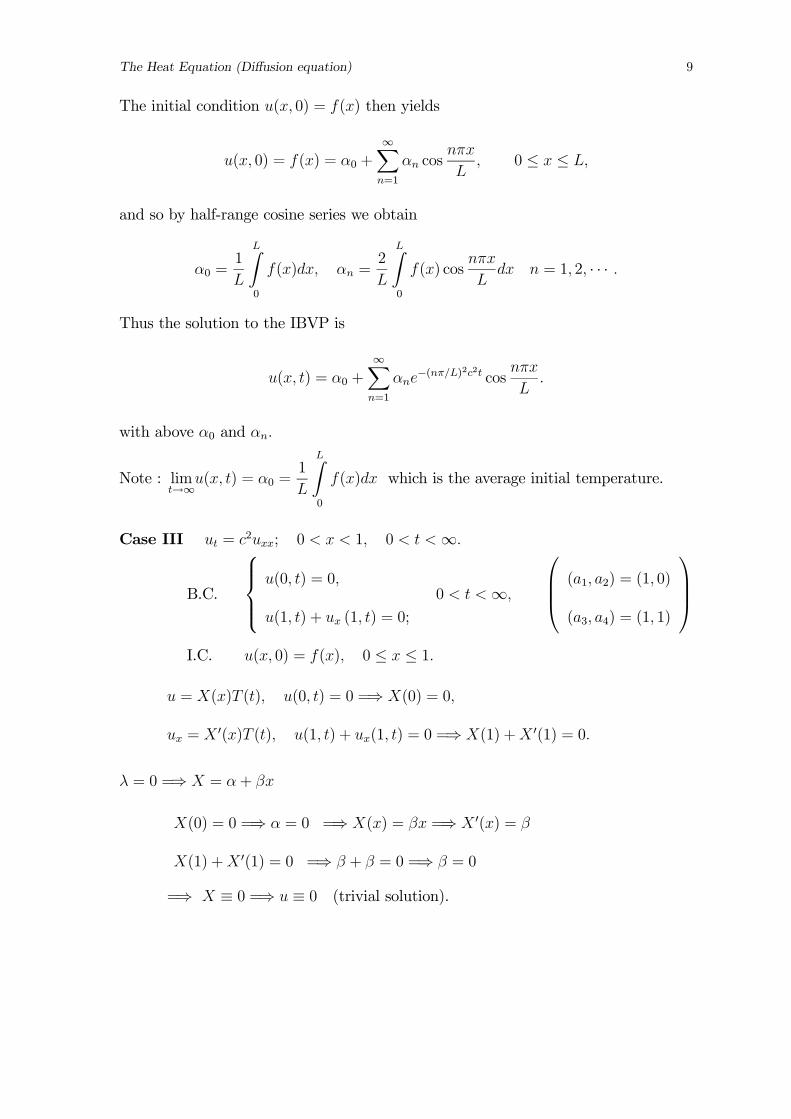
The Heat Equation (Diffusion equation) 9

The initial condition u(x, 0) = f(x) then yields

u(x, 0) = f(x) = α0 +∞Xn=1

αn cosnπx

L, 0 ≤ x ≤ L,

and so by half-range cosine series we obtain

α0 =1

L

LZ0

f(x)dx, αn =2

L

LZ0

f(x) cosnπx

Ldx n = 1, 2, · · · .

Thus the solution to the IBVP is

u(x, t) = α0 +∞Xn=1

αne−(nπ/L)2c2t cos

nπx

L.

with above α0 and αn.

Note : limt→∞

u(x, t) = α0 =1

L

LZ0

f(x)dx which is the average initial temperature.

Case III ut = c2uxx; 0 < x < 1, 0 < t <∞.

B.C.

u(0, t) = 0,

u(1, t) + ux (1, t) = 0;

0 < t <∞,

(a1, a2) = (1, 0)

(a3, a4) = (1, 1)

I.C. u(x, 0) = f(x), 0 ≤ x ≤ 1.

u = X(x)T (t), u(0, t) = 0 =⇒ X(0) = 0,

ux = X 0(x)T (t), u(1, t) + ux(1, t) = 0 =⇒ X(1) +X 0(1) = 0.

λ = 0 =⇒ X = α+ βx

X(0) = 0 =⇒ α = 0 =⇒ X(x) = βx =⇒ X 0(x) = β

X(1) +X 0(1) = 0 =⇒ β + β = 0 =⇒ β = 0

=⇒ X ≡ 0 =⇒ u ≡ 0 (trivial solution).

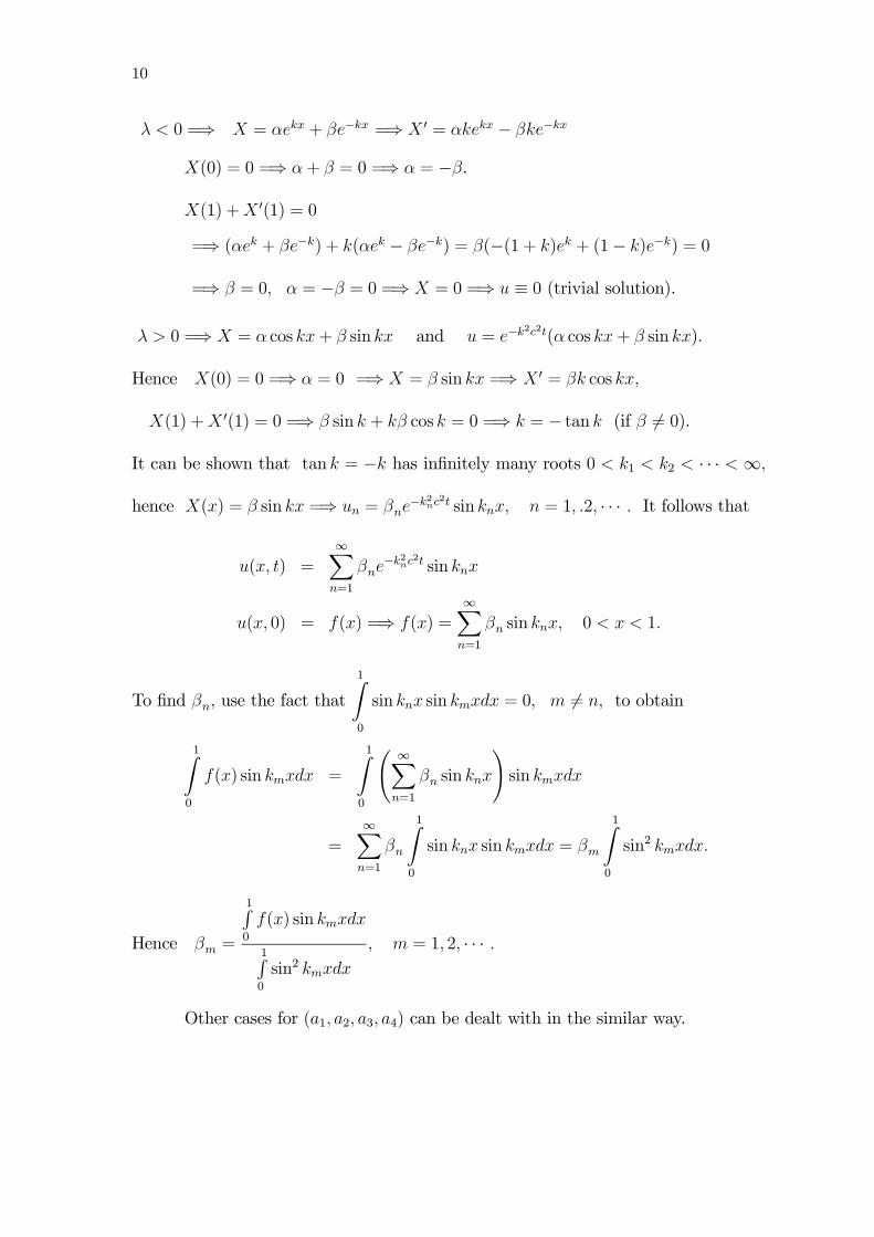
10

λ < 0 =⇒ X = αekx + βe−kx =⇒ X 0 = αkekx − βke−kx

X(0) = 0 =⇒ α+ β = 0 =⇒ α = −β.

X(1) +X 0(1) = 0

=⇒ (αek + βe−k) + k(αek − βe−k) = β(−(1 + k)ek + (1− k)e−k) = 0

=⇒ β = 0, α = −β = 0 =⇒ X = 0 =⇒ u ≡ 0 (trivial solution).

λ > 0 =⇒ X = α cos kx+ β sin kx and u = e−k2c2t(α cos kx+ β sin kx).

Hence X(0) = 0 =⇒ α = 0 =⇒ X = β sin kx =⇒ X 0 = βk cos kx,

X(1) +X 0(1) = 0 =⇒ β sin k + kβ cos k = 0 =⇒ k = − tan k (if β 6= 0).

It can be shown that tan k = −k has infinitely many roots 0 < k1 < k2 < · · · <∞,

hence X(x) = β sin kx =⇒ un = βne−k2nc2t sin knx, n = 1, .2, · · · . It follows that

u(x, t) =∞Xn=1

βne−k2nc2t sin knx

u(x, 0) = f(x) =⇒ f(x) =∞Xn=1

βn sin knx, 0 < x < 1.

To find βn, use the fact that

1Z0

sin knx sin kmxdx = 0, m 6= n, to obtain

1Z0

f(x) sin kmxdx =

1Z0

à ∞Xn=1

βn sin knx

!sin kmxdx

=∞Xn=1

βn

1Z0

sin knx sin kmxdx = βm

1Z0

sin2 kmxdx.

Hence βm =

1R0

f(x) sin kmxdx

1R0

sin2 kmxdx

, m = 1, 2, · · · .

Other cases for (a1, a2, a3, a4) can be dealt with in the similar way.

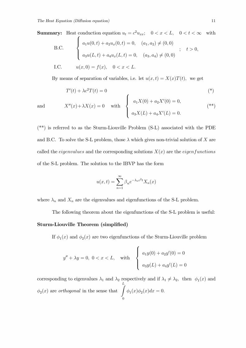
The Heat Equation (Diffusion equation) 11

Summary: Heat conduction equation ut = c2uxx; 0 < x < L, 0 < t <∞ with

B.C.

a1u(0, t) + a2ux(0, t) = 0, (a1, a2) 6= (0, 0)

a3u(L, t) + a4ux(L, t) = 0, (a3, a4) 6= (0, 0); t > 0,

I.C. u(x, 0) = f(x), 0 < x < L.

By means of separation of variables, i.e. let u(x, t) = X(x)T (t), we get

T 0(t) + λc2T (t) = 0 (*)

and X 00(x)+λX(x) = 0 with

a1X(0) + a2X

0(0) = 0,

a3X(L) + a4X0(L) = 0.

(**)

(**) is referred to as the Sturm-Liouville Problem (S-L) associated with the PDE

and B.C. To solve the S-L problem, those λ which gives non-trivial solution of X are

called the eigenvalues and the corresponding solutions X(x) are the eigenfunctions

of the S-L problem. The solution to the IBVP has the form

u(x, t) =∞Xn=1

βne−λnc2tXn(x)

where λn and Xn are the eigenvalues and eigenfunctions of the S-L problem.

The following theorem about the eigenfunctions of the S-L problem is useful:

Sturm-Liouville Theorem (simplified)

If φ1(x) and φ2(x) are two eigenfunctions of the Sturm-Liouville problem

y00 + λy = 0, 0 < x < L, with

a1y(0) + a2y

0(0) = 0

a3y(L) + a4y0(L) = 0

corresponding to eigenvalues λ1 and λ2 respectively and if λ1 6= λ2, then φ1(x) and

φ2(x) are orthogonal in the sense that

LZ0

φ1(x)φ2(x)dx = 0.

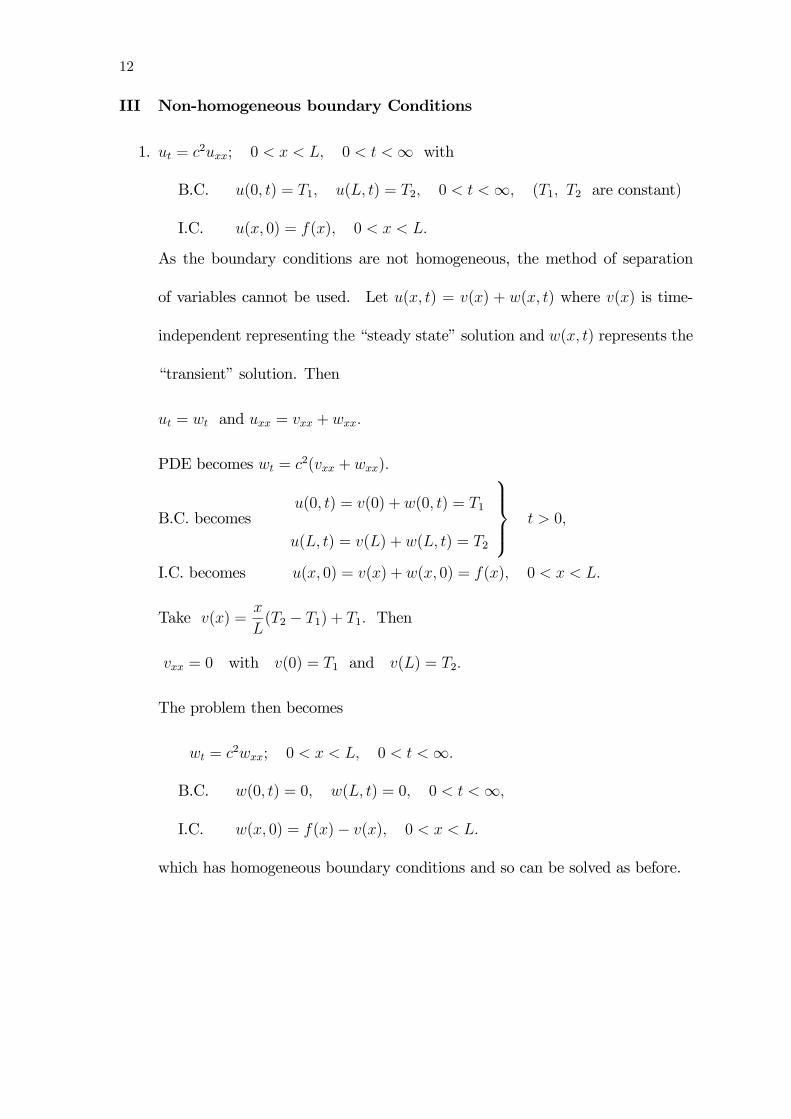
12

III Non-homogeneous boundary Conditions

1. ut = c2uxx; 0 < x < L, 0 < t <∞ with

B.C. u(0, t) = T1, u(L, t) = T2, 0 < t <∞, (T1, T2 are constant)

I.C. u(x, 0) = f(x), 0 < x < L.

As the boundary conditions are not homogeneous, the method of separation

of variables cannot be used. Let u(x, t) = v(x) + w(x, t) where v(x) is time-

independent representing the “steady state” solution and w(x, t) represents the

“transient” solution. Then

ut = wt and uxx = vxx + wxx.

PDE becomes wt = c2(vxx + wxx).

B.C. becomesu(0, t) = v(0) + w(0, t) = T1

u(L, t) = v(L) + w(L, t) = T2

t > 0,

I.C. becomes u(x, 0) = v(x) + w(x, 0) = f(x), 0 < x < L.

Take v(x) =x

L(T2 − T1) + T1. Then

vxx = 0 with v(0) = T1 and v(L) = T2.

The problem then becomes

wt = c2wxx; 0 < x < L, 0 < t <∞.

B.C. w(0, t) = 0, w(L, t) = 0, 0 < t <∞,

I.C. w(x, 0) = f(x)− v(x), 0 < x < L.

which has homogeneous boundary conditions and so can be solved as before.

Non-homogeneous boundary Conditions 13

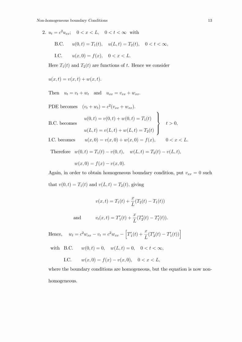
2. ut = c2uxx; 0 < x < L, 0 < t <∞ with

B.C. u(0, t) = T1(t), u(L, t) = T2(t), 0 < t <∞,

I.C. u(x, 0) = f(x), 0 < x < L.

Here T1(t) and T2(t) are functions of t. Hence we consider

u(x, t) = v(x, t) + w(x, t).

Then ut = vt + wt and uxx = vxx + wxx.

PDE becomes (vt + wt) = c2(vxx + wxx).

B.C. becomesu(0, t) = v(0, t) + w(0, t) = T1(t)

u(L, t) = v(L, t) + w(L, t) = T2(t)

t > 0,

I.C. becomes u(x, 0) = v(x, 0) + w(x, 0) = f(x), 0 < x < L.

Therefore w(0, t) = T1(t)− v(0, t), w(L, t) = T2(t)− v(L, t),

w(x, 0) = f(x)− v(x, 0).

Again, in order to obtain homogeneous boundary condition, put vxx = 0 such

that v(0, t) = T1(t) and v(L, t) = T2(t), giving

v(x, t) = T1(t) +x

L(T2(t)− T1(t))

and vt(x, t) = T 01(t) +x

L(T 02(t)− T 01(t)).

Hence, wt = c2wxx − vt = c2wxx −hT 01(t) +

x

L(T 02(t)− T 01(t))

iwith B.C. w(0, t) = 0, w(L, t) = 0, 0 < t <∞,

I.C. w(x, 0) = f(x)− v(x, 0), 0 < x < L,

where the boundary conditions are homogeneous, but the equation is now non-

homogeneous.

14

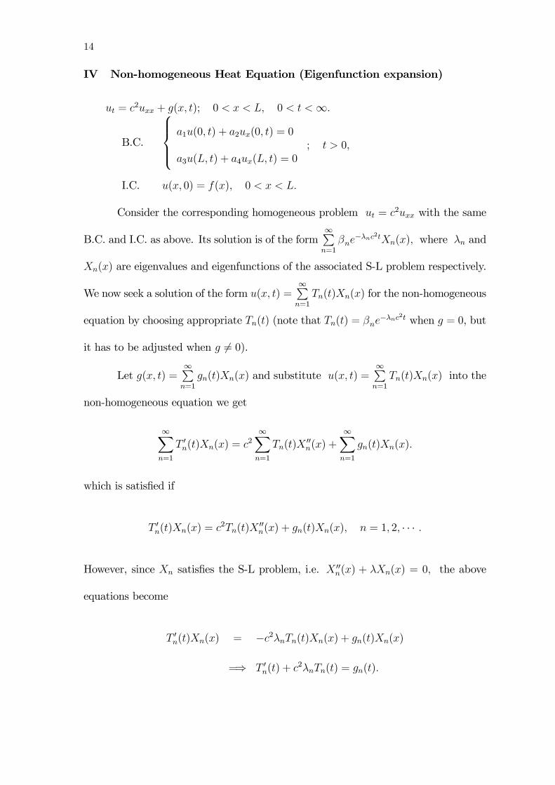
IV Non-homogeneous Heat Equation (Eigenfunction expansion)

ut = c2uxx + g(x, t); 0 < x < L, 0 < t <∞.

B.C.

a1u(0, t) + a2ux(0, t) = 0

a3u(L, t) + a4ux(L, t) = 0; t > 0,

I.C. u(x, 0) = f(x), 0 < x < L.

Consider the corresponding homogeneous problem ut = c2uxx with the same

B.C. and I.C. as above. Its solution is of the form∞Pn=1

βne−λnc2tXn(x), where λn and

Xn(x) are eigenvalues and eigenfunctions of the associated S-L problem respectively.

We now seek a solution of the form u(x, t) =∞Pn=1

Tn(t)Xn(x) for the non-homogeneous

equation by choosing appropriate Tn(t) (note that Tn(t) = βne−λnc2t when g = 0, but

it has to be adjusted when g 6= 0).

Let g(x, t) =∞Pn=1

gn(t)Xn(x) and substitute u(x, t) =∞Pn=1

Tn(t)Xn(x) into the

non-homogeneous equation we get

∞Xn=1

T 0n(t)Xn(x) = c2∞Xn=1

Tn(t)X00n(x) +

∞Xn=1

gn(t)Xn(x).

which is satisfied if

T 0n(t)Xn(x) = c2Tn(t)X00n(x) + gn(t)Xn(x), n = 1, 2, · · · .

However, since Xn satisfies the S-L problem, i.e. X 00n(x) + λXn(x) = 0, the above

equations become

T 0n(t)Xn(x) = −c2λnTn(t)Xn(x) + gn(t)Xn(x)

=⇒ T 0n(t) + c2λnTn(t) = gn(t).

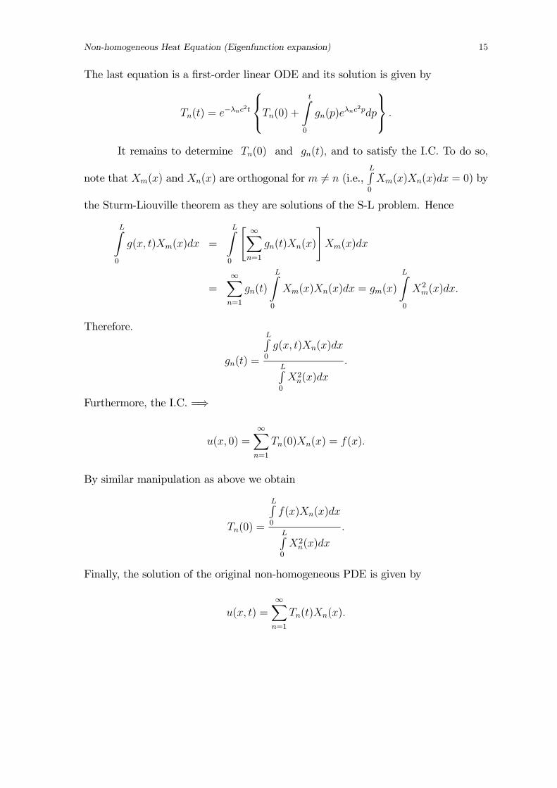
Non-homogeneous Heat Equation (Eigenfunction expansion) 15

The last equation is a first-order linear ODE and its solution is given by

Tn(t) = e−λnc2t

Tn(0) +

tZ0

gn(p)eλnc2pdp

.

It remains to determine Tn(0) and gn(t), and to satisfy the I.C. To do so,

note that Xm(x) and Xn(x) are orthogonal for m 6= n (i.e.,LR0

Xm(x)Xn(x)dx = 0) by

the Sturm-Liouville theorem as they are solutions of the S-L problem. Hence

LZ0

g(x, t)Xm(x)dx =

LZ0

" ∞Xn=1

gn(t)Xn(x)

#Xm(x)dx

=∞Xn=1

gn(t)

LZ0

Xm(x)Xn(x)dx = gm(x)

LZ0

X2m(x)dx.

Therefore.

gn(t) =

LR0

g(x, t)Xn(x)dx

LR0

X2n(x)dx

.

Furthermore, the I.C. =⇒

u(x, 0) =∞Xn=1

Tn(0)Xn(x) = f(x).

By similar manipulation as above we obtain

Tn(0) =

LR0

f(x)Xn(x)dx

LR0

X2n(x)dx

.

Finally, the solution of the original non-homogeneous PDE is given by

u(x, t) =∞Xn=1

Tn(t)Xn(x).

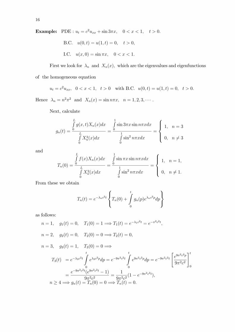
16

Example: PDE : ut = c2uxx + sin 3πx, 0 < x < 1, t > 0.

B.C. u(0, t) = u(1, t) = 0, t > 0,

I.C. u(x, 0) = sinπx, 0 < x < 1.

First we look for λn and Xn(x), which are the eigenvalues and eigenfunctions

of the homogeneous equation

ut = c2uxx, 0 < x < 1, t > 0 with B.C. u(0, t) = u(1, t) = 0, t > 0.

Hence λn = n2π2 and Xn(x) = sinnπx, n = 1, 2, 3, · · · .

Next, calculate

gn(t) =

LR0

g(x, t)Xn(x)dx

LR0

X2n(x)dx

=

1R0

sin 3πx sinnπxdx

1R0

sin2 nπxdx

=

1, n = 3

0, n 6= 3

and

Tn(0) =

LR0

f(x)Xn(x)dx

LR0

X2n(x)dx

=

1R0

sinπx sinnπxdx

1R0

sin2 nπxdx

=

1, n = 1,

0, n 6= 1.

From these we obtain

Tn(t) = e−λnc2t

Tn(0) +

tZ0

gn(p)eλnc2pdp

as follows:

n = 1, g1(t) = 0, T1(0) = 1 =⇒ T1(t) = e−λ1c2t = e−π

2c2t,

n = 2, g2(t) = 0, T2(0) = 0 =⇒ T2(t) = 0,

n = 3, g3(t) = 1, T3(0) = 0 =⇒

T3(t) = e−λ3c2t

tZ0

eλ3c2pdp = e−9π

2c2t

tZ0

e9π2c2pdp = e−9π

2c2t

"e9π

2c2p

9π2c2

#t0

=e−9π

2c2t(e9π2c2t − 1)

9π2c2=

1

9π2c2(1− e−9π

2c2t),

n ≥ 4 =⇒ gn(t) = Tn(0) = 0 =⇒ Tn(t) = 0.

More Heat Conduction Equations 17

Finally, we obtain the solution as

u(x, t) = T1(t)X1(x) + T3(t)X3(x)

= e−π2c2t sinπx+

1

9π2c2(1− e−9π

2c2t) sin 3πx.

V More Heat Conduction Equations

ut = c2uxx − αu; 0 < x < 1, 0 < t <∞.

B.C. u(0, t) = u(1, t) = 0; t > 0,

I.C. u(x, 0) = f(x), 0 ≤ x ≤ 1,where −αu represents heat flow across the lateral boundary.

As diffusion along the x direction is represented by c2uxx, the term −αu would

affect the solution in t only.

Let u(x, t) = φ(t)w(x, t). Then

ut = φwt + φtw and uxx = φwxx.

Therefore PDE =⇒ φwt + φtw = c2φwxx − αφw

=⇒ wt = c2wxx −µα+

φtφ

¶w.

Let φt/φ = −α. Then φt + αφ = 0 =⇒ φ = e−αt and the PDE becomes

wt = c2wxx

with B.C. w(0, t) = w(1, t) = 0

I.C. w(x, 0) = f(x).

Thus w(x, t) may be obtained as previously and u(x, t) = e−αtw(x, t).

18

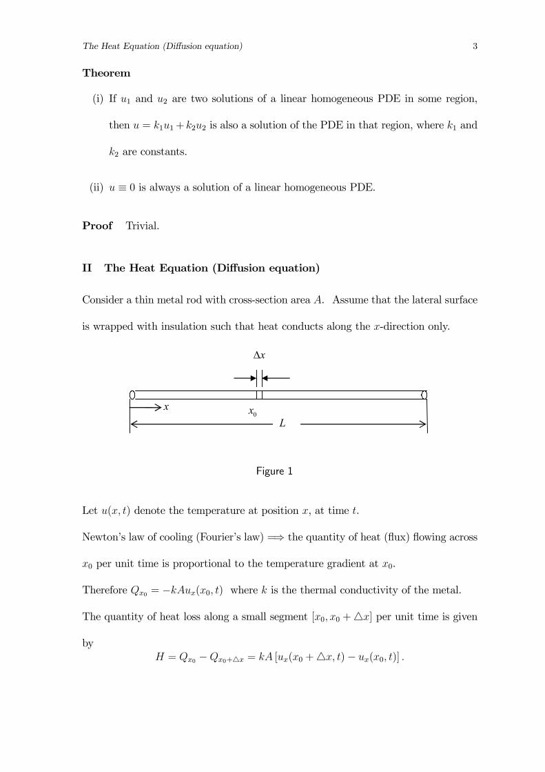
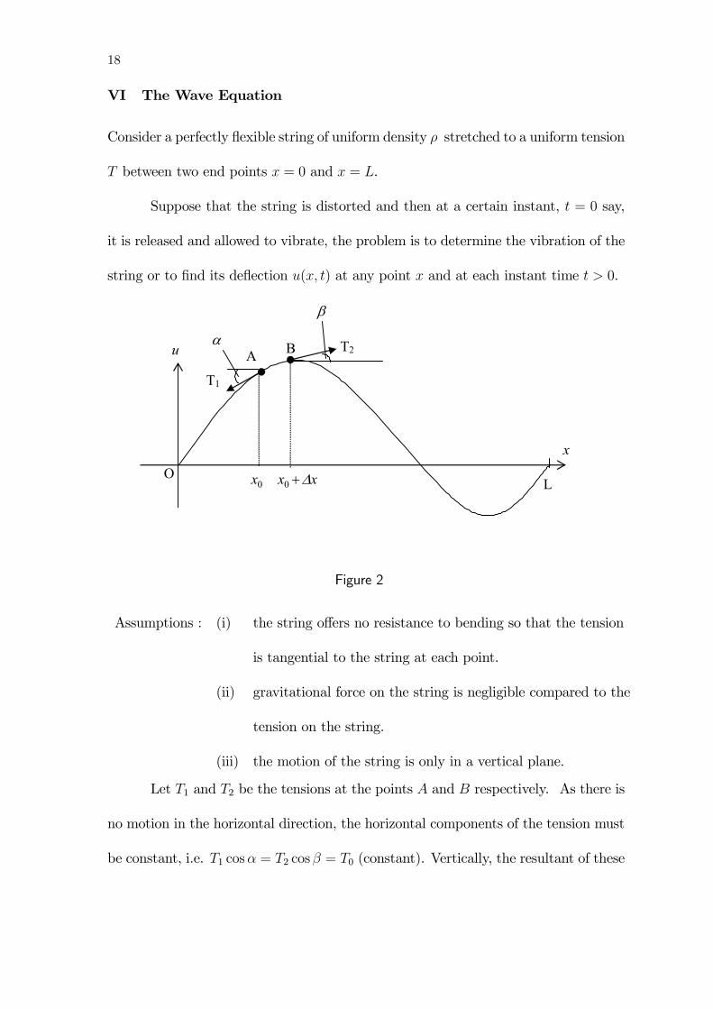
VI The Wave Equation

Consider a perfectly flexible string of uniform density ρ stretched to a uniform tension

T between two end points x = 0 and x = L.

Suppose that the string is distorted and then at a certain instant, t = 0 say,

it is released and allowed to vibrate, the problem is to determine the vibration of the

string or to find its deflection u(x, t) at any point x and at each instant time t > 0.

u

x

xxx ∆+00

T2

T1

A B

L O

α

β

Figure 2

Assumptions : (i) the string offers no resistance to bending so that the tension

is tangential to the string at each point.

(ii) gravitational force on the string is negligible compared to the

tension on the string.

(iii) the motion of the string is only in a vertical plane.

Let T1 and T2 be the tensions at the points A and B respectively. As there is

no motion in the horizontal direction, the horizontal components of the tension must

be constant, i.e. T1 cosα = T2 cosβ = T0 (constant). Vertically, the resultant of these

The Wave Equation 19

forces leads to the vertical vibration of the string and

Newton’s 2nd law =⇒ T2 sinβ − T1 sinα = ρδxutt

(ρδx is the mass of the string between A and B).

It follows that

tanβ − tanα = T2 sinβ

T2 cosβ− T1 sinα

T1 cosα=

ρδx

T0utt.

As tanβ = ux(B, t) = ux(x+ δx, t) and tanα = ux(A, t) = ux(x, t), we get

1

δx[ux(x+ δx, t)− ux(x, t)] =

ρ

T0utt.

Letting δx → 0 =⇒ uxx =ρ

T0utt =⇒ utt = c2uxx (c2 = T0/ρ), which is called

the wave equation.

IBVP for Wave equation

PDE: utt = c2uxx; 0 < x < L, t > 0.

B.C. u(0, t) = u(L, t) = 0, t > 0,

I.C.

u(x, 0) = f(x)

ut(x, 0) = g(x)

, 0 < x < L.

By the method of separation of variables, take u(x, t) = X(x)T (t). Then

utt = c2uxx =⇒ X(x)T 00(t) = c2X 00(x)T (t) =⇒T 00(t)c2T (t)

=X 00(x)X(x)

= −λ (constant) =⇒

(i)X 00(x) + λX(x) = 0

X(0) = X(L) = 0

associated Sturm-Liouville problem

(ii) T 00(t) + c2λT (t) = 0.

20

(i) =⇒ λn =n2π2

L2; Xn(x) = sin

nπx

L, n = 1, 2, · · ·

(ii) =⇒ Tn(t) = αn cosnπc

Lt+ βn sin

nπc

Lt.

Therefore the solution is given by

u(x, t) =∞Pn=1

³αn cos

nπc

Lt+ βn sin

nπc

Lt´sin

nπx

L,

u(x, 0) = f(x) =⇒ αn =2

L

LZ0

f(x) sinnπx

Ldx,

ut(x, 0) = g(x) =⇒ βn =2

nπc

LZ0

g(x) sinnπx

Ldx.

Note that αn cosnπc

Lt+βn sin

nπc

Lt = γn cos

hnπcL(t+ φn)

i(where γn =

pα2n + β2n

and φn =L

nπcarctan

αn

βn). Hence the solution may also be expressed as

u(x, t) =∞Xn=1

γn coshnπcL(t+ φn)

isin

nπx

L.

VII Classification of 2nd order linear PDE in 2 independent variables

Consider the 2nd order linear PDE

A(x, y)uxx+B(x, y)uxy+C(x, y)uyy+D(x, y)ux+E(x, y)ux+F (x, y)u = G(x, y) (∗)

If B2 − 4AC > 0 for (x, y) ∈ Ω ⊂ R2, (∗) is said to be hyperbolic in Ω.

If B2 − 4AC < 0 for (x, y) ∈ Ω ⊂ R2, (∗) is said to be elliptic in Ω.

If B2 − 4AC = 0 for (x, y) ∈ Ω ⊂ R2, (∗) is said to be parabolic in Ω.

Example utt = c2uxx =⇒ c2uxx − utt = 0. Let y = t. Then A = c2, B = 0,

C = −1. Hence B2 − 4AC = 4c2 > 0. Thus the wave equation is hyperbolic.

For ut = c2uxx, A = c2, B = C = 0, so B2 − 4AC = 0. Hence the heat equation is

parabolic.

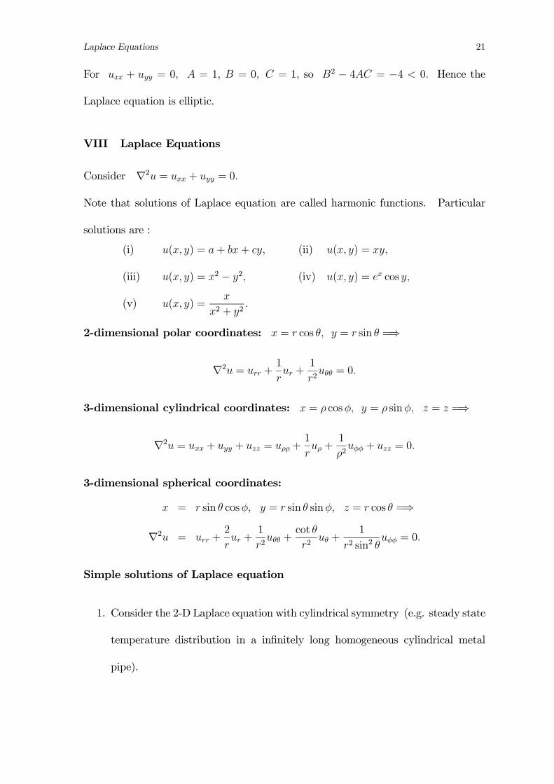
Laplace Equations 21

For uxx + uyy = 0, A = 1, B = 0, C = 1, so B2 − 4AC = −4 < 0. Hence the

Laplace equation is elliptic.

VIII Laplace Equations

Consider ∇2u = uxx + uyy = 0.

Note that solutions of Laplace equation are called harmonic functions. Particular

solutions are :

(i) u(x, y) = a+ bx+ cy, (ii) u(x, y) = xy,

(iii) u(x, y) = x2 − y2, (iv) u(x, y) = ex cos y,

(v) u(x, y) =x

x2 + y2.

2-dimensional polar coordinates: x = r cos θ, y = r sin θ =⇒

∇2u = urr +1

rur +

1

r2uθθ = 0.

3-dimensional cylindrical coordinates: x = ρ cosφ, y = ρ sinφ, z = z =⇒

∇2u = uxx + uyy + uzz = uρρ +1

ruρ +

1

ρ2uφφ + uzz = 0.

3-dimensional spherical coordinates:

x = r sin θ cosφ, y = r sin θ sinφ, z = r cos θ =⇒

∇2u = urr +2

rur +

1

r2uθθ +

cot θ

r2uθ +

1

r2 sin2 θuφφ = 0.

Simple solutions of Laplace equation

1. Consider the 2-D Laplace equation with cylindrical symmetry (e.g. steady state

temperature distribution in a infinitely long homogeneous cylindrical metal

pipe).

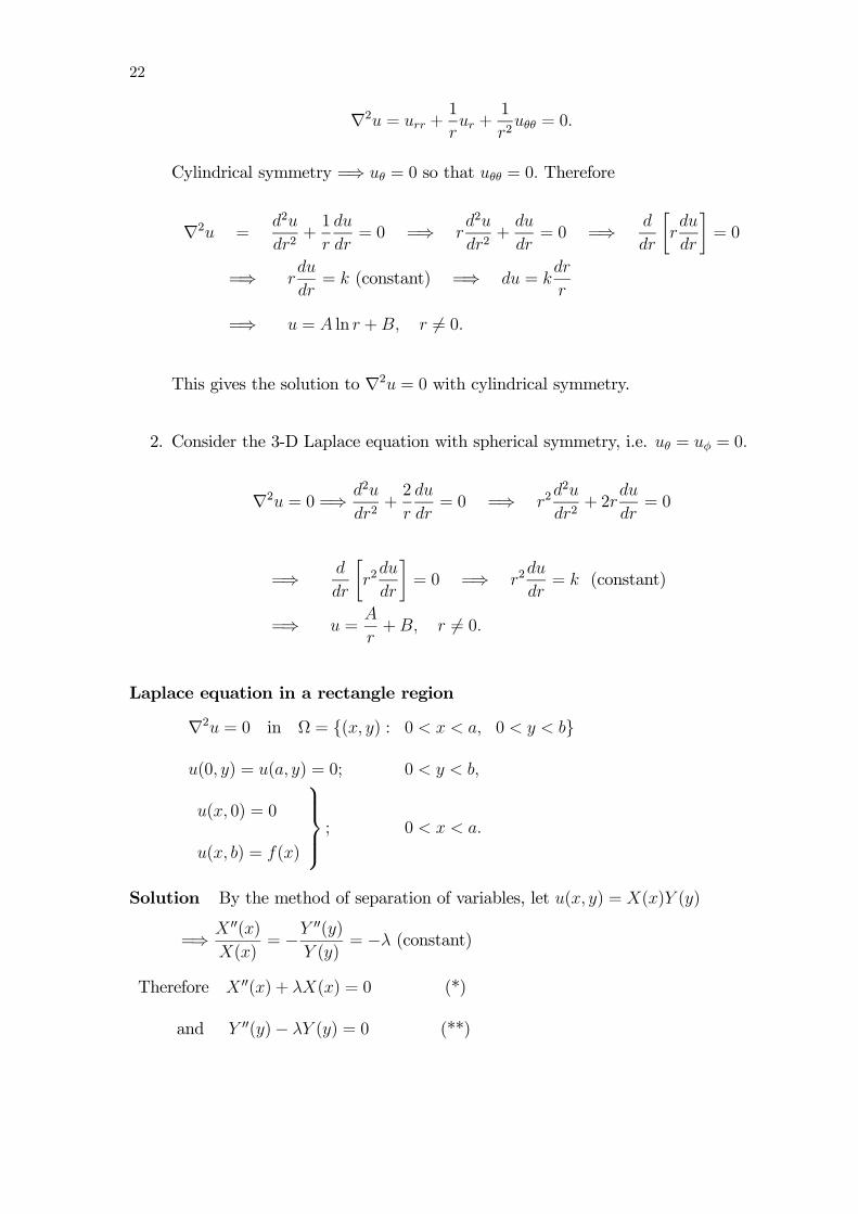
22

∇2u = urr +1

rur +

1

r2uθθ = 0.

Cylindrical symmetry =⇒ uθ = 0 so that uθθ = 0. Therefore

∇2u =d2u

dr2+1

r

du

dr= 0 =⇒ r

d2u

dr2+

du

dr= 0 =⇒ d

dr

·rdu

dr

¸= 0

=⇒ rdu

dr= k (constant) =⇒ du = k

dr

r

=⇒ u = A ln r +B, r 6= 0.

This gives the solution to ∇2u = 0 with cylindrical symmetry.

2. Consider the 3-D Laplace equation with spherical symmetry, i.e. uθ = uφ = 0.

∇2u = 0 =⇒ d2u

dr2+2

r

du

dr= 0 =⇒ r2

d2u

dr2+ 2r

du

dr= 0

=⇒ d

dr

·r2du

dr

¸= 0 =⇒ r2

du

dr= k (constant)

=⇒ u =A

r+B, r 6= 0.

Laplace equation in a rectangle region

∇2u = 0 in Ω = (x, y) : 0 < x < a, 0 < y < b

u(0, y) = u(a, y) = 0; 0 < y < b,

u(x, 0) = 0

u(x, b) = f(x)

; 0 < x < a.

Solution By the method of separation of variables, let u(x, y) = X(x)Y (y)

=⇒ X 00(x)X(x)

= −Y00(y)

Y (y)= −λ (constant)

Therefore X 00(x) + λX(x) = 0 (*)

and Y 00(y)− λY (y) = 0 (**)

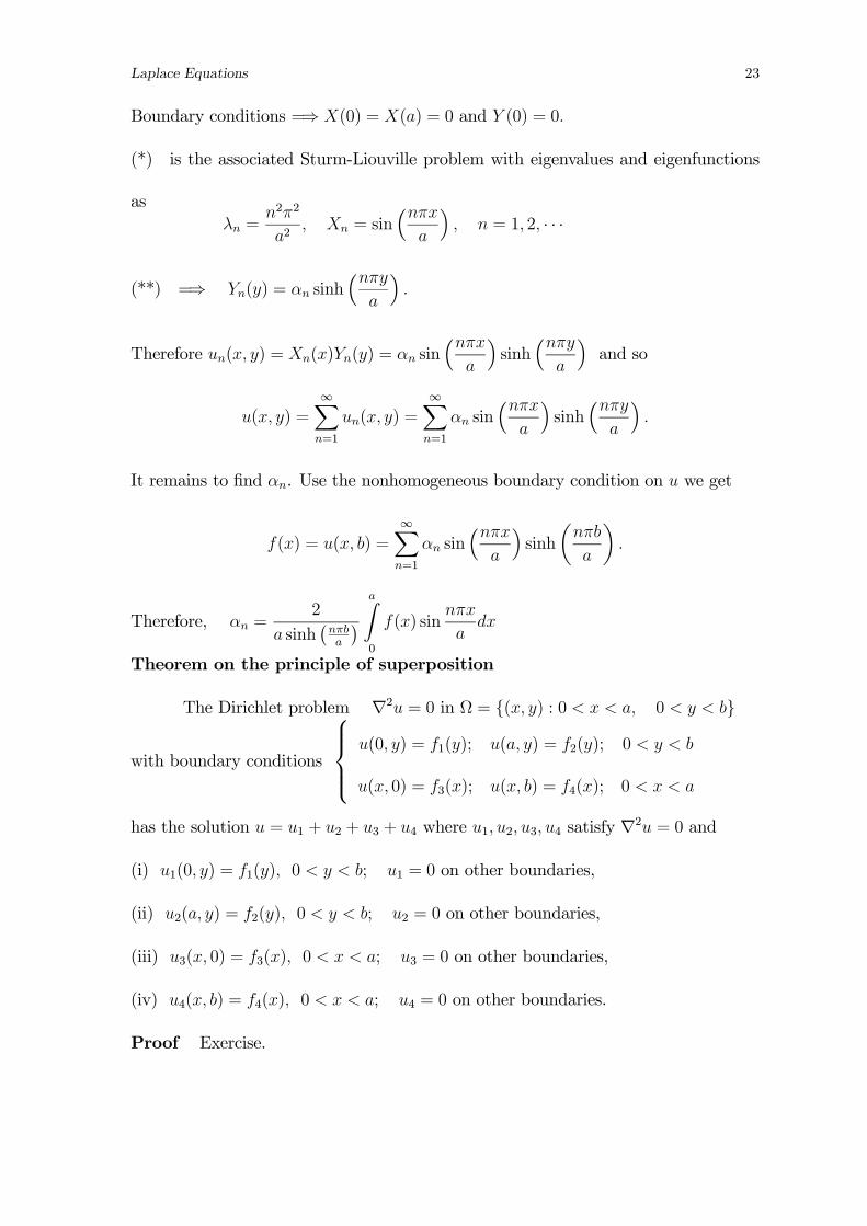
Laplace Equations 23

Boundary conditions =⇒ X(0) = X(a) = 0 and Y (0) = 0.

(*) is the associated Sturm-Liouville problem with eigenvalues and eigenfunctions

asλn =

n2π2

a2, Xn = sin

³nπxa

´, n = 1, 2, · · ·

(**) =⇒ Yn(y) = αn sinh³nπy

a

´.

Therefore un(x, y) = Xn(x)Yn(y) = αn sin³nπx

a

´sinh

³nπya

´and so

u(x, y) =∞Xn=1

un(x, y) =∞Xn=1

αn sin³nπx

a

´sinh

³nπya

´.

It remains to find αn. Use the nonhomogeneous boundary condition on u we get

f(x) = u(x, b) =∞Xn=1

αn sin³nπx

a

´sinh

µnπb

a

¶.

Therefore, αn =2

a sinh¡nπba

¢ aZ0

f(x) sinnπx

adx

Theorem on the principle of superposition

The Dirichlet problem ∇2u = 0 in Ω = (x, y) : 0 < x < a, 0 < y < b

with boundary conditions

u(0, y) = f1(y); u(a, y) = f2(y); 0 < y < b

u(x, 0) = f3(x); u(x, b) = f4(x); 0 < x < a

has the solution u = u1 + u2 + u3 + u4 where u1, u2, u3, u4 satisfy ∇2u = 0 and

(i) u1(0, y) = f1(y), 0 < y < b; u1 = 0 on other boundaries,

(ii) u2(a, y) = f2(y), 0 < y < b; u2 = 0 on other boundaries,

(iii) u3(x, 0) = f3(x), 0 < x < a; u3 = 0 on other boundaries,

(iv) u4(x, b) = f4(x), 0 < x < a; u4 = 0 on other boundaries.

Proof Exercise.

24

Laplace equation in circular regions

∇2u = 0 in Ω = (x, y) : x2 + y2 < A,

u(x, y) = f(x, y) on the of boundary of .Ω.

In polar coordinates, the equation becomes ∇2u = urr +1

rur +

1

r2uθθ = 0,

and the boundary condition becomes u(A, θ) = f(θ), 0 < θ < 2π.

Note that u(r, θ) is periodic in θ of period 2π and is bounded as r → 0.

Let u(r, θ) = R(r)Θ(θ) and substitute it into the equation we obtain

R00Θ+1

rR0Θ+

1

r2RΘ00 = 0 =⇒ r2

R00

R+ r

R0

R= −Θ

00

Θ= −λ (constant)

which leads to (i) Θ00 + λΘ = 0, Θ(θ) is periodic with period 2π.

(ii) r2R00 + rR0 − λR = 0, limr→0

R(r) <∞.

For (i), λ = 0 =⇒ Θ(θ) = α+ βθ and Θ(θ) is periodic =⇒ β = 0 =⇒ Θ(θ) = α.

λ < 0 (λ = −k2) =⇒ Θ = αekθ + βe−kθ and

Θ(θ) is periodic =⇒ α = β = 0 =⇒ Θ(θ) ≡ 0 (trivial solution).

λ > 0 (λ = k2) =⇒ Θ = α cos kθ + β sin kθ and

Θ(θ) is periodic with period 2π =⇒ k = n = 1, 2, · · · .

Therefore we get a sequence of solutions for Θ(θ) as

Θ0(θ) = α0, Θn(θ) = αn cosnθ + βn sinnθ; n = 1, 2, · · · .

For (ii), λ = 0 =⇒ r2R00 + rR0 = 0 =⇒ rR00 +R0 = 0 =⇒ (rR0)0 = 0

=⇒ rR0 = c1 =⇒ R = c2 + c1 ln r.

However, limr→0

R(r) <∞ =⇒ c1 = 0 =⇒ R(r) = c2.

λ = k2 = n2 =⇒ r2R00 + rR0 − n2R = 0 (Euler equation)

Let R = rm and by substitution into Euler equation we get m = ±n.

Thus R(r) = c3rn + c4r

−n and limr→0

R(r) <∞ =⇒ c4 = 0 =⇒ R(r) = Rn(r) = rn.

Laplace Equations 25

It follows that un(r, θ) = Θn(θ)Rn(r) = rn(αn cosnθ + βn sinnθ); n = 0, 1, 2, · · · .

By the principle of superposition,

u(r, θ) = α0 +∞Xn=1

rn(αn cosnθ + βn sinnθ)

where αn and βn are determined from the boundary conditions

u(A, θ) = f(θ) =⇒ f(θ) = α0 +∞Xn=1

An(αn cosnθ + βn sinnθ),

which leads to α0 =1

2π

Z 2π

0

f(θ)dθ,

αn =1

πAn

Z 2π

0

f(θ) cosnθdθ (n = 1, 2, ...),

βn =1

πAn

Z 2π

0

f(θ) sinnθdθ (n = 1, 2, ...).

*******************************

Reference Books:

Kreyszig E., Advanced Engineering Mathematics, Wiley International Edition.

Farlow S.J., Partial Differential Equations for Scientists and Engineers, Wiley Inter-

national Edition.

Boyce W.E. and DiPrima R.C., Elementary Differential Equations and Boundary

Value Problems, Wiley International Edition.

Derrick W.R. and Grossman S.I., Elementary Differential Equations with Boundary

Value Problems, Addison Wesley.