Embed Size (px)
Citation preview

University of Nottingham
Investigating the Value of Postponement in Inventory Routing Problems
Fernando Saka Herrán
MSc Operations Management

Investigating the Value of Postponement in Inventory Routing Problems
By
Fernando Saka Herrán
2009
A dissertation presented in part consideration for the degree of
MSc Operations Management

Investigating the Value of Postponement in Inventory Routing Problems
III
ACKNOWLEDGEMENTS
Foremost, I would like to show my gratitude to my supervisor Dr. Luc Muyldermans, who
shared with me a lot of his expertise and research insight about vehicle routing problems.
Moreover, I would like to thank him for the reason that he made available his support even
though I realized this dissertation in Chile.
Thanks a lot to the University of Nottingham, the staff and teachers, for providing me this
exceptional opportunity to study in the UK.
I owe my deepest appreciation to my family, specially my mother who has been an
unconditional support not only during this process but also throughout my entire life.
Finally, I would like to dedicate this dissertation to my beloved father Fernando Saka
Santostasio.

Investigating the Value of Postponement in Inventory Routing Problems
IV
TABLE OF CONTENTS
ABSTRACT ....................................................................................................................... VIII
1. INTRODUCTION ............................................................................................................ 1
1.1. Research Aim and Objectives ................................................................................. 2
1.2. Research Methodology .......................................................................................... 2
1.3. Dissertation Structure ............................................................................................ 3
2. LITERATURE REVIEW .................................................................................................... 4
2.1. Vehicle Routing Problem (VRP) .............................................................................. 4
2.1.1. Representation of the Vehicle Routing Problem ............................................... 5
2.1.2. Classification of Vehicle Routing Problems ....................................................... 5
2.1.2.1. Nature of Delivery Time ............................................................................ 6
2.1.2.2. Degree of Dynamism................................................................................. 6
2.1.2.3. Nature of Cost .......................................................................................... 6
2.1.3. Characteristics of Vehicle Routing Problems ..................................................... 7
2.1.3.1. Size of Available Fleet ............................................................................... 7
2.1.3.2. Type of Available Fleet .............................................................................. 8
2.1.3.3. Housing Vehicles ....................................................................................... 8
2.1.3.4. Nature of Demand .................................................................................... 8
2.1.3.5. Location of Demand .................................................................................. 8
2.1.3.6. Underlying Network.................................................................................. 8
2.1.3.7. Vehicle Capacity Restrictions ..................................................................... 8
2.1.3.8. Maximum Route Times ............................................................................. 9
2.1.3.9. Crew Requirements .................................................................................. 9
2.1.3.10. Data Requirements ................................................................................. 9
2.1.3.11. Operations.............................................................................................. 9
2.1.3.12. Costs ...................................................................................................... 9
2.1.3.13. Objectives............................................................................................. 10

Investigating the Value of Postponement in Inventory Routing Problems
V
2.1.4. Variants of Vehicle Routing Problem .............................................................. 10
2.1.4.1. Capacitated Vehicle Routing Problem (CVRP)........................................... 10
2.1.4.2. Distance-Constrained Vehicle Routing Problem (DVRP) ............................ 10
2.1.4.3. Distance-Constrained Capacitated Vehicle Routing Problem (DCVRP) ....... 11
2.1.4.4. Multiple Depot Vehicle Routing Problem (MDVRP) .................................. 11
2.1.4.5. Periodic Vehicle Routing Problem (PVRP) ................................................ 11
2.1.4.6. Split Delivery Vehicle Routing Problem (SDVRP) ...................................... 12
2.1.4.7. Stochastic Vehicle Routing Problem (SVRP) ............................................. 12
2.1.4.8. Vehicle Routing Problem with Satellite Facilities (VRPSF) ......................... 13
2.1.4.9. Vehicle Routing Problem with Backhauls (VRPB) ...................................... 13
2.1.4.10. Vehicle Routing Problem with Pick-Up and Delivery (VRPPD) ................. 14
2.1.4.11. Vehicle Routing Problem with Time Windows (VRPTW) ......................... 15
2.2. Inventory Routing Problem (IRP) .......................................................................... 15
2.3. Postponement Horizon/Accumulation Time (t) ..................................................... 16
2.4. Continuous Approximation Theory (CA) ............................................................... 18
3. EXPERIMENT DESIGN .................................................................................................. 20
3.1. Experiment Assumptions ..................................................................................... 20
3.2. Experiment Parameters ....................................................................................... 20
3.2.1. Service Region (A) ......................................................................................... 20
3.2.2. Depot Location .............................................................................................. 22
3.2.3. Customers Demand Rate (r) ........................................................................... 23
3.2.4. Customers’ Density (n) .................................................................................. 23
3.2.5. Vehicle Capacity (Q) ...................................................................................... 24
3.2.6. Summary ...................................................................................................... 25
3.3. Experiment Costs ................................................................................................. 25
3.3.1. Radial Routing Cost ....................................................................................... 25
3.3.1.1. Average Line-Haul Distance for Scenarios A, B and C ................................ 26
3.3.1.2. Average Line-Haul Distance for Scenarios D and E .................................... 27

Investigating the Value of Postponement in Inventory Routing Problems
VI
3.3.1.3. Average Line-Haul Distance for Scenarios F and G .................................... 28
3.3.1.4. Summary ................................................................................................ 29
3.3.2. Local Routing Cost ......................................................................................... 29
3.3.3. Inventory Holding Cost .................................................................................. 30
3.3.4. Total Cost ...................................................................................................... 30
3.4. Experiment Diagrams ........................................................................................... 31
3.4.1. Routing Cost Curves ...................................................................................... 31
3.4.2. Inventory Holding Cost Surface Diagrams ....................................................... 31
3.4.3. Total Cost Surface Diagrams .......................................................................... 31
3.4.4. Optimal Postponement Horizon Curves ......................................................... 31
3.5. Experiment Scenarios .......................................................................................... 32
3.5.1. Scenario A ..................................................................................................... 32
3.5.2. Scenario B ..................................................................................................... 33
3.5.3. Scenario C ..................................................................................................... 33
3.5.4. Scenario D ..................................................................................................... 33
3.5.5. Scenario E ..................................................................................................... 33
3.5.6. Scenario F ..................................................................................................... 33
3.5.7. Scenario G ..................................................................................................... 33
3.5.8. Summary ...................................................................................................... 34
4. EXPERIMENT RESULTS ................................................................................................ 35
4.1. Scenario A Results ............................................................................................... 36
4.2. Scenario B Results ................................................................................................ 38
4.3. Scenario C Results ................................................................................................ 40
4.4. Scenario D Results ............................................................................................... 40
4.5. Scenario E Results ................................................................................................ 43
4.6. Scenario F Results ................................................................................................ 44
4.7. Scenario G Results ............................................................................................... 46
4.8. Summary ............................................................................................................. 47

Investigating the Value of Postponement in Inventory Routing Problems
VII
4.9. Figures ................................................................................................................ 50
5. EXPERIMENT DISCUSSION........................................................................................... 67
5.1. Service Region (A) Impact .................................................................................... 67
5.2. Depot Location Impact ......................................................................................... 69
5.3. Customers Demand Rate (r) Impact ...................................................................... 70
5.4. Customers Density (n) Impact .............................................................................. 71
6. CONCLUSION.............................................................................................................. 72
7. REFERENCES ............................................................................................................... 74
8. APPENDICES ............................................................................................................... 78

Investigating the Value of Postponement in Inventory Routing Problems
VIII
ABSTRACT
Transportation and inventory management account for a large portion of the costs of
distribution companies, so postponing delivery services could result in savings in these
expenses.
This particular study focuses on finding the optimal postponement horizon in which both
routing and inventory holding costs are minimized. In addition, the research aims to explore
the impact of a variety of parameters (service area, depot location, customers demand rate,
customers density and vehicle capacity) in the optimal accumulation times and inventory
routing costs.
For diverse routing scenarios, several problem instances are created in excel. Results are
obtained by using a continuous approximation model. Finally, through a graphical analysis, the
key findings about the optimal level of postponement are revealed.
This paper concludes that the optimal level of postponement in inventory routing problems
depends on the combination of the problem parameters. Optimal postponement horizons are
shorter for cases when the inventory holding costs dominates the routing costs, when the
vehicle capacity decreases, when the depot is centrally located, when the customers are
located in service regions near the depot and when the customers demand rate is
independent. Yet, optimal postponement horizons are larger under reverse conditions.

Investigating the Value of Postponement in Inventory Routing Problems
1
1. INTRODUCTION
Nowadays the globalization leads all the productive sectors to evolve day after day in order to
become competitive firms. This arises as a consequence of the great competence combined
with the demand and the requirements of the customers searching for quality, flexibility,
rapidity, functionality and low costs in their products. Thereupon, one of the principal
problems that companies must deal with is the implementation of an effective and efficient
logistic value chain.
By definition, a logistic strategy is a set of means and necessary methods to carry out the
organization of a distribution company or distribution service. Moreover, through the logistic
process a wide range of costs and entities are involved. Suppliers, manufacturers and
distribution centers are constantly performing several activities with the intention of reducing
not only the material and manufacturing costs but also the transportations costs and the
inventory holding costs, while customers are uniformly distributed around a defined service
region waiting to be served.
Figure 1.1. Logistic Supply Chain
Source: Simchi-Levi D et al. (2000)

Investigating the Value of Postponement in Inventory Routing Problems
2
One of the key activities of logistics is the transportation of commodities from a distribution
center to a broad number of customers. Effective transportation means that customers are
served with the right product, at the right place, at the right time and in the right quantity.
Hence, for companies is imperative to have the minimum possible routing and inventory
holding costs to become competitive in the market.
This dissertation focuses in the reduction of these costs by finding the optimal level of
postponement in diverse inventory routing situations.
1.1. Research Aim and Objectives
The purpose of this study is to find the optimal trade-off between routing costs and inventory
holding costs in different scenarios. In other words, several inventory routing instances are
created in excel to determine the optimal postponement horizon in which both routing and
inventory holding costs are reduced. Moreover, the research aims to reveal which is the
impact of a variety of parameters in the optimal accumulation times and inventory routing
costs. The parameters are,
Service region (A)
Depot location
Customers demand rate (r)
Customers’ density (n)
Vehicle capacity (Q)
1.2. Research Methodology
The research methodology is based on a quantitative method in which a mathematical model
is employed to collect and analyze data. Three main steps are involved in the quantitative
research procedure. In the first place, several routing instances are created in excel. Secondly,
a continuous approximation theory is applied to examine each of the routing scenarios. Finally,
through a numerical and graphical analysis, results and conclusions over the parameters are
exposed.

Investigating the Value of Postponement in Inventory Routing Problems
3
1.3. Dissertation Structure
The dissertation is structured in the following sections,
Chapter 2 provides a review of the main aspects in vehicle routing problems. VRPs
classification, characteristics and variants are explained to understand the main
difference with inventory routing problems. Furthermore, an overview on
postponement is shown and a brief description on the continuous approximation
theory used to run the experiments is revealed.
Chapter 3 describes the problem. Specifically, this section covers the assumptions
made, the parameters and costs involved, and the graphs developed to analyze the
different experiment instances. Besides, an outline of the different scenarios created is
given.
Chapter 4 presents the results obtained in the different routing instances.
Chapter 5 discusses the impact of each of the parameters involved in the problem.
Chapter 6 entails the conclusions and recommends future research areas.

Investigating the Value of Postponement in Inventory Routing Problems
4
2. LITERATURE REVIEW
2.1. Vehicle Routing Problem (VRP)
Real world applications concerning the delivery of specific goods from a single depot to a wide
range of clients was introduced in 1959 by Dantzig and Ramser. The first mathematical
programming formulation and algorithmic approach described the optimal designing of routes
to deliver gasoline from a central depot to a number of service stations. Since the problem was
established, several models and algorithms have been proposed to reach the optimal solution
of the different variety of the vehicle routing problem. For detailed overview of a
computational algorithm see Clarke and Wright (1964).
By definition, the vehicle routing problem seeks to minimize the global transportation costs by
defining a set of routes that are passed through by a single vehicle fulfilling all the customers’
requirements. Moreover, the vehicle starts and ends at the same depot, visiting each customer
once and satisfying the operational constraints (Toth and Vigo, 2002). Toth and Vigo (2002)
argue that there are four main objectives considered by a VRP. These are,
1. Minimization of global transportation cost.
2. Minimization of the number of vehicles or drivers required to serve all customers.
3. Balancing the routes, for travel time and vehicle load.
4. Minimization of the penalties associated with partial service of the customers.
According to Woensel T et al. (2008) the most important constraints that need to be satisfied
in order to obtain these objectives in a practical VRP are,
1. Every vehicle route has a total demand constrained by the vehicle capacity Q. For
example if the vehicle capacity is 10 units, then the total demand of every vehicle
route can have a maximum value of 10 units.
2. Every vehicle route has a total route length constrained by the route length L. For
example if the route length is 100 metres, then the vehicle route can have a maximum
distance of 100 metres.

Investigating the Value of Postponement in Inventory Routing Problems
5
2.1.1. Representation of the Vehicle Routing Problem
The vehicle routing problem can be represented by a graph G = (V, A, c). V symbolizes the set
of vertices (V = 0, 1…n), A the set of arcs (A = {(i, j) : i<>j}) and c, the non-negative cost that is
associated to the distance travelled from a vertex i to a vertex j. Furthermore, each customer
has a non-negative service time di and a non-negative demand qdi given as an initial constraint
to the problem. Frequently, these values are equal to 0 (Woensel T et al., 2008).
Following figure shows the depot, the routes and customers in a VRP.
Figure 2.1. Vehicle Routing Problem
Source: Web Reference 2
2.1.2. Classification of Vehicle Routing Problems
Vehicle routing problems can be classified in different ways depending on the approach the
problem is given. As the main output of VRPs is commonly the same, characteristics and
assumptions about the problem have to be analyzed in order to distinguish the diversity in
which VRPs can be classified. Based on nature of delivery time, on degree of dynamism and on
nature of cost, vehicle routing problems have different variants.

Investigating the Value of Postponement in Inventory Routing Problems
6
2.1.2.1. Nature of Delivery Time
Bodin L et al. (1983) subdivided the VRP depending on the nature of delivery time of goods
from the depot to the customers. This division contained three main groups,
1. Routing problems
2. Scheduling problems
3. Routing and scheduling problems
Routing and scheduling problems differ in temporal considerations. On one hand, those that
do not take into account delivery time constraints are defined as routing problems. In fact,
ignoring temporal considerations assumes that customers can be served in a short period of
time without any restrictions. On the other hand, those that are restricted are defined as
scheduling problems. The combination of routing and scheduling problems allows for temporal
and spatial (precedence relationship) requirements.
2.1.2.2. Degree of Dynamism
In accordance with Larsen A (2000) the vehicle routing problem can be classified depending on
the degree of dynamism. If the input data is known, then it is a static VRP. For example in a
dial-a-ride system, the passenger is picked up at the initial location and transported to the final
destination. On the contrary, if the input data changes over short periods of time, then it is a
dynamic VRP. For example in a taxi cab service the destination can change with a simple
request of the customer.
2.1.2.3. Nature of Cost
Cordeau J F et al. (2007) argue that vehicle routing problems can be divided into two
categories depending on the nature of cost of the problem. These are,
1. Symmetric vehicle routing problem
2. Asymmetric vehicle routing problem
A graph G = (V, A) can be directed either undirected depending if the arcs that connects the
vertices have a clear direction or not. In an undirected graph, a vertex has no sense of

Investigating the Value of Postponement in Inventory Routing Problems
7
direction. Therefore, cost will be symmetric and hence the VRP will be symmetric. On the
other hand, if G is a directed graph, the cost will be asymmetric and consequently the VRP will
be asymmetric as well.
To understand better the difference between undirected graphs with directed graphs, Allison L
(1999) provided two illustrations,
Figure 2.2. Undirected Graph Figure 2.3. Directed Graph
Source: Allison L (1999) Source: Allison L (1999)
2.1.3. Characteristics of Vehicle Routing Problems
As the vehicle routing problem is a combinatorial optimization of tasks to improve or reduce
the total transportation costs, several features arise from its main components. Vehicle
capacity, location of the depot, set of crews (drivers), road network and customers are defined
as the key components in a vehicle routing problem and so forth it is necessary to understand
the different characteristics in order to cope with the objective of the VRP.
According to Bodin L et al. (1983) and Golden and Assad (1988) the characteristics and possible
options in terms of the main components are the following.
2.1.3.1. Size of Available Fleet
1. One vehicle.
2. Multiple vehicles.

Investigating the Value of Postponement in Inventory Routing Problems
8
2.1.3.2. Type of Available Fleet
1. Homogeneous (one vehicle type).
2. Heterogeneous (multiple vehicle types).
3. Special vehicle types (compartmentalized, etc).
2.1.3.3. Housing Vehicles
1. Single depot.
2. Multiple depots.
2.1.3.4. Nature of Demand
1. Deterministic demand (known).
2. Stochastic demand (not known).
3. Partial satisfaction of demand allowed.
2.1.3.5. Location of Demand
1. At nodes (not necessary all).
2. At arcs (not necessary all).
3. Mixed.
2.1.3.6. Underlying Network
1. Directed.
2. Undirected.
3. Mixed.
4. Euclidean.
2.1.3.7. Vehicle Capacity Restrictions
1. Imposed (all the same or different vehicle capacities).
2. Unlimited capacity.
Investigating the Value of Postponement in Inventory Routing Problems
9
2.1.3.8. Maximum Route Times
1. Imposed (same for all routes).
2. Imposed (different for different routes).
3. Not imposed.
2.1.3.9. Crew Requirements
1. Fixed number of drivers.
2. Variable number of drivers.
3. Mixed (fixed and variable number of drivers).
2.1.3.10. Data Requirements
1. Geographic database, road networks.
2. Customer addresses and locations.
3. Travel times.
4. Vehicle location information.
5. Customer credit and billing information.
2.1.3.11. Operations
1. Pickups only.
2. Deliveries only.
3. Mixed (pickups and deliveries).
4. Split deliveries (allowed or disallowed).
2.1.3.12. Costs
1. Variable or routing costs.
2. Fixed operating or vehicle acquisition costs.
3. Common carrier costs (for unserviced demands).

Investigating the Value of Postponement in Inventory Routing Problems
10
2.1.3.13. Objectives
1. Minimize total routing costs.
2. Minimize sum of fixed and variable costs.
3. Minimize number of vehicles required.
4. Maximize utility function based on service or convenience.
5. Maximize utility function based on customer priorities.
2.1.4. Variants of Vehicle Routing Problem
Depending on the combination of the component characteristics, diverse variants arise from
the essential vehicle routing problem. For example if the vehicle capacity is imposed, then the
problem is known as capacitated vehicle routing problem and thus the parameters change as
well as the operational constraints and customers’ requirements.
Web Reference 2 and Toth and Vigo (2002) presented different variants of the VRP. These are,
2.1.4.1. Capacitated Vehicle Routing Problem (CVRP)
The capacitated VRP is known as the basic version of the VRP. Actually, the only difference is
that every vehicle is required to have uniform capacity of a single commodity and the sum of
the demand of all customers for the commodity on a single route must not exceed the vehicle
capacity (Guneri A F, 2007).
Application environment for CVRP includes solid waste collection, beverage, food and
newspaper industries (Toth and Vigo, 2002).
2.1.4.2. Distance-Constrained Vehicle Routing Problem (DVRP)
In this case, the difference is that every single route traversed by a vehicle should not exceed
the imposed length route (Woensel T et al., 2008).

Investigating the Value of Postponement in Inventory Routing Problems
11
2.1.4.3. Distance-Constrained Capacitated Vehicle Routing Problem (DCVRP)
Those problems with distance and capacity constraints are called distance-constrained
capacitated VRPs (Toth and Vigo, 2002).
2.1.4.4. Multiple Depot Vehicle Routing Problem (MDVRP)
Normally, customers are dispersed around a single depot that satisfies their demands. In a
multiple depot VRP, customers are served by several depots in order to minimize routing costs
(Crevier B et al., 2007).
Figure 2.4. Multiple Depot Vehicle Routing Problem
Source: Web Reference 1
2.1.4.5. Periodic Vehicle Routing Problem (PVRP)
The periodic VRP deals with problems that occur to companies which have to perform
deliveries of goods in a periodic horizon. In a first phase this variant of the VRP tries to assign
each customer a different period of supply to then minimize the total routing cost. In fact, the
objective of the PVRP is to minimize total transportation cost over the planning horizon (Coene
S et al., 2008).
Practical applications of PVRP are in the soft drink industry (vending machines) and automotive
industry (part distribution). For detailed overview on PVRP see Francis P et al. (2006).
Investigating the Value of Postponement in Inventory Routing Problems
12
2.1.4.6. Split Delivery Vehicle Routing Problem (SDVRP)
The vehicle routing problem with split delivery refers to instances where the same customer
can be served by different vehicles if the total transportation costs are reduced. This means
that customers demand can be divided between several vehicles (Chen S et al., 2007).
Real world applications of SDVRP involve routing of helicopters in the North Sea, crew
exchanges and commercial sanitation collection (Chen S et al., 2007).
2.1.4.7. Stochastic Vehicle Routing Problem (SVRP)
A stochastic problem is one whose parameters are non-deterministic and the solution is
determined not only by predictable actions but also by random elements. Therefore, the SVRP
according to Gendreau M et al. (1996) is a VRP where one or several components of the
problem are random. To deal with these uncertainties, three different variants exist depending
if the uncertain parameter is the customer location, demand or travel time. These are,
1. Vehicle Routing Problem with Stochastic Customers (VRPSC).
2. Vehicle Routing Problem with Stochastic Demands (VRPSD).
3. Vehicle Routing Problem with Stochastic Travel Times (VRPSTT).
Kleywegt A J et al. (2000) argue that there are two necessary phases in order to obtain a
feasible solution in a stochastic VRP. In the first place, a solution is taken without knowing the
random parameters. In the second and final stage, the solution is achieved by using in an
iterative way the parameters obtained in the first part. A third phase could be necessary to
reach a more accurate solution by using the parameters obtained in the second phase.
Active applications of the SVRP are the daily demand for cash at a bank's automatic teller
machine and the volume of trash at each stop on a waste collection route.

Investigating the Value of Postponement in Inventory Routing Problems
13
2.1.4.8. Vehicle Routing Problem with Satellite Facilities (VRPSF)
An extension where the vehicle can be replenished during a route is called VRPs with satellite
facilities. In fact, satellite replenishment allows the drivers of the vehicles to carry on making
deliveries without returning to the central depot (Web Reference 3).
Distribution of fuels and retail stores are two real life applications of the VRPSF.
2.1.4.9. Vehicle Routing Problem with Backhauls (VRPB)
Vehicle routing problems in which customers can demand or return some commodities is
commonly known as VRP with backhauls. This variant of the VRP is mainly an extension of the
CVRP where the customer set V\ {0} is divided into two parts, the linehaul customers and the
backhaul customers. Linehaul customers are those that require a given quantity of product to
be delivered and the backhaul customers are those where a given quantity of inbound product
must be picked up. Although linehaul and backhaul customers are independent, there is a
precedence constraint in which linehaul customers must be served before any backhaul
customer (Toth and Vigo, 2002).
Figure 2.5. Vehicle Routing Problem with Backhauls
Source: Web Reference 3
Investigating the Value of Postponement in Inventory Routing Problems
14
Some real life examples of vehicle routing problems with backhauls include the grocery
industry where supermarkets and shops are the linehaul customers and grocery suppliers are
the backhaul customers (Toth and Vigo, 2002).
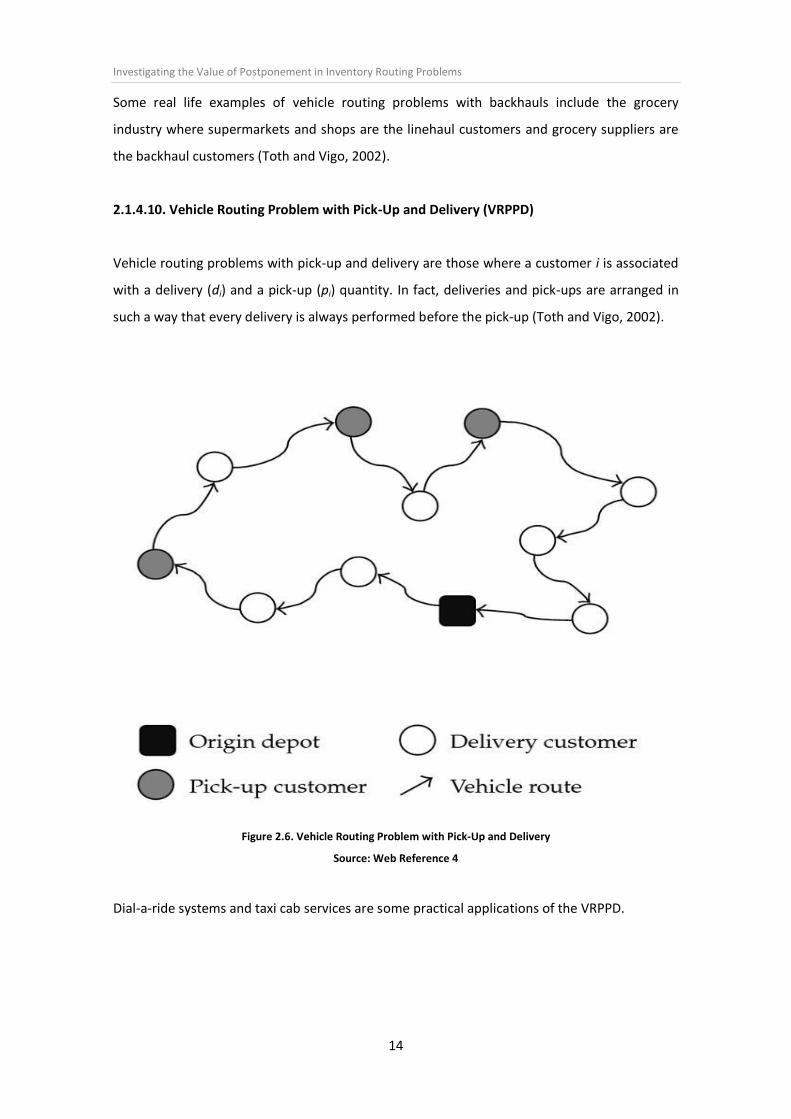
2.1.4.10. Vehicle Routing Problem with Pick-Up and Delivery (VRPPD)
Vehicle routing problems with pick-up and delivery are those where a customer i is associated
with a delivery (di) and a pick-up (pi) quantity. In fact, deliveries and pick-ups are arranged in
such a way that every delivery is always performed before the pick-up (Toth and Vigo, 2002).
Figure 2.6. Vehicle Routing Problem with Pick-Up and Delivery
Source: Web Reference 4
Dial-a-ride systems and taxi cab services are some practical applications of the VRPPD.

Investigating the Value of Postponement in Inventory Routing Problems
15
2.1.4.11. Vehicle Routing Problem with Time Windows (VRPTW)
Vehicle routing problems in which capacity constraints are imposed and each customer i has a
time interval are known as VRPs with time windows. The time window is the time instant
involved since the vehicle departs from the depot until it serves the customer. Normally,
vehicles leave the depot at time instant 0 and arrive to customers at a time t defined by the
time window. Furthermore, if the vehicle arrives early to the customer, it is allowed to wait
until time instant t (Toth and Vigo, 2002).
Practical examples of VRPTW include postal deliveries, national franchise restaurant services
and security patrol services (Toth and Vigo, 2002).
2.2. Inventory Routing Problem (IRP)
The inventory routing problem is defined as an extension of the VRP. Besides, IRP is considered
a more challenging and intriguing problem for the reason that integrates different components
of the logistics value chain such as transportation and inventory management. For decades,
production and transportation have been treated separately; hence the IRP is nowadays a
positive approach to solve problems incurring not only routing costs but also inventory holding
costs (Campbell A et al., 1997).
In general terms, inventory routing problems differ in two aspects from the vehicle routing
problem. In the first place, VRPs delivery time is reduced to a single day where all orders have
to be delivered by the end of the day. On the contrary in inventory routing problems,
deliveries are scheduled over a planning horizon without causing stockouts at any of the
customers. The second difference is that in vehicle routing problems orders are requested by
customers and in IRPs, the delivery company decides the frequency of the order and the
delivery amount served to each customer (Toth and Vigo, 2002). Therefore, the inventory
routing problem tries to design the set of routes that will minimize transportation costs and
inventory holding costs (Chen and Lin, 2009).
Formally, the main objective of IRPs is to find the adequate trade-off between routing costs
(proportional to distance travelled) and inventory holding cost (proportional to the average
Investigating the Value of Postponement in Inventory Routing Problems
16
level of inventory). According to Campbell A et al. (1997) three decisions must be made to
obtain a feasible solution,
When to serve a customer?
How much to deliver to a customer when served?
Which delivery routes to use?
Although all proposed solution approaches to solve inventory routing problems are short term
versions, IRPs are considered long term planning problems in a given planning horizon in view
of the fact that demand is stochastic in nature. Due to this uncertainty, Chen and Lin (2009)
argue that two aspects should be solved within the planning horizon,
How to model the long term effect of short term decisions?
Which customers to include in the short-term planning period?
Vendor managed inventory replenishment deals with these uncertainties. Indeed, VMI is a
business practice in which the supplier manages the inventory replenishment of the customers
creating a win-win situation (suppliers minimizes distribution costs and customers avoids the
use of resources to inventory management).
Logistics chains using IRPs strategies such as vendor managed inventory include aerospace
industry, automotive industry, food and beverage industries, metal production industry,
retailers and petroleum industry (Campbell A et al., 1997).
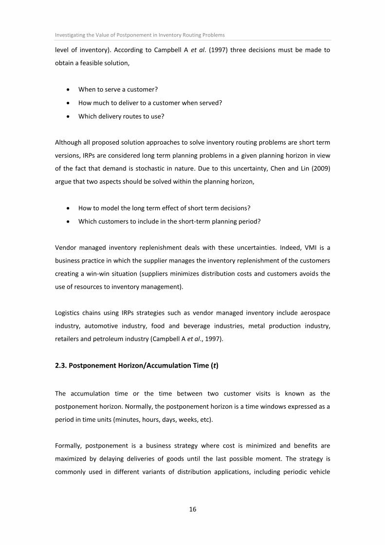
2.3. Postponement Horizon/Accumulation Time (t)
The accumulation time or the time between two customer visits is known as the
postponement horizon. Normally, the postponement horizon is a time windows expressed as a
period in time units (minutes, hours, days, weeks, etc).
Formally, postponement is a business strategy where cost is minimized and benefits are
maximized by delaying deliveries of goods until the last possible moment. The strategy is
commonly used in different variants of distribution applications, including periodic vehicle

Investigating the Value of Postponement in Inventory Routing Problems
17
routing problems, inventory routing problems, waste collection management and reverse
logistics (Muyldermans and Pang, 2009).
Beullens et al. (2004) analyzed the value of postponement in reverse logistics developing a
continuous approximation model to see the impact of postponement under different
integration policies (backhauling and mixing) in a vehicle routing problem with pick-up and
delivery. The study exposed that the optimal level of postponement is directly related to
different parameters such as the location of the depot or the customers’ density. Furthermore,
the analysis concluded that in some cases a non-postponed policy was more efficient and in
other cases a maximum postponement policy was the optimal solution to the problem
reducing the routing costs in a 20%.
Muyldermans and Pang (2009) studied the impact of postponing routing decisions in a
capacitated vehicle routing problem in which the customer demands occur over a certain
period of time and the supplier in charge of the service can decide when to visit the customers.
The analysis revealed that postponement has a positive effect in the reduction of the routing
costs. Besides, as the experiment analyzed by Beullens et al. (2004), the investigation showed
that postponement is completely related to parameters like the location of the depot, the
vehicle capacity and the customers’ density.
In waste collection, there is evidence that using a postponed strategy helps to reduce the total
routing costs. For example in the city of Mesa (Arizona), the waste collection was reduced from
twice per week to once per week, minimizing not only the routing costs but also the labour
costs and demand over time. In addition, in 1995 in the Montgomery County (Maryland), two
service rates (twice per week and once per week) were implemented in order to reduce the
costs in the collection of residential waste. Results showed that a service rate of once per week
reduced the routing costs in a 70% (Muyldermans and Pang, 2009).
In this dissertation, a maximum postponement strategy is used to find the optimal
accumulation times in which both routing and inventory holding costs are reduced. Maximum
postponement means that the distribution of commodities is performed in the maximum
possible time horizon. i.e., maximum accumulation time = tmax.

Investigating the Value of Postponement in Inventory Routing Problems
18
2.4. Continuous Approximation Theory (CA)
Continuous approximation models are considered the opposite to discrete models in modern
logistic applications. The main characteristic of these models is that the optimal solution is
approximately reached by identifying sensitivities of the near optimal without performing
exhaustive computational experiments (Daganzo C F, 2005). Originally, the CA method was
proposed by Newell (1971) and the main goal was to obtain a feasible solution with as little
information as possible, gaining a deep insight into trade-offs that affect real world situations.
Campbell J F (1996) argues that a continuous approximation model consists on iterative
estimation of different parameters including costs, demand rate, customers’ density, vehicle
capacity and depot location. Erratic evaluations of these parameters can take to
underestimations or overestimations of the problem under discussion. Consequently, Daganzo
C F (2005) suggests that the variation of these parameters must be measured in order to see
optimal results.
According to Daganzo C F (1984a, 1984b) a good approximation formula for the total distance
travelled by vehicles with a specific capacity Q, servicing n customers in a service region with
area A is,
Anqq
nl )(2
The term l2 n/q denotes the total radial distance, with l as the average line-haul distance
(distance between the depot and the customers), n as the number of customers and q as the
number of customers served in a route. On the contrary, the term Anq)( is an
approximation of the total local routing distance (distance between two customers), with )(q
as a constant depending on the Euclidean metric (distance between two points given by
22),( yxyxd ) and the number of customers served on each tour, A as the service area
and n as the number of customers.

Investigating the Value of Postponement in Inventory Routing Problems
19
In accordance with Campbell J F (1993) the constant )(q can take the following values,
)(q = 0.57, when 6q
)(q = 0.6, when 5q
)(q = 0.63, when 4q
)(q = 0.68, when 3q
)(q = 0.73, when 2q
)(q = 0, when 1q
For detailed overview on how the expression was worked out see Daganzo C F (1984a, 1984b,
2005).

Investigating the Value of Postponement in Inventory Routing Problems
20
3. EXPERIMENT DESIGN
Inventory routing problems can either be solved by exact models or by analytical models. In
this case, a continuous approximation technique proposed by Daganzo C F (1984a, 1984b,
2005) is applied in diverse scenarios to distinguish the influence of diverse parameters in IRPs.
Furthermore, the main objective of this paper is to reveal until which point postponed delivery
frequencies can minimize the total costs without carrying out detailed computational
experiments.
This chapter involves the assumptions, parameters, costs, diagrams and scenarios of the
experiment.
3.1. Experiment Assumptions
The problem has five main assumptions,
1. Demand of the customers is known at all time by the service provider (no demand
uncertainty).
2. Customers are uniformly distributed inside the service region.
3. Each customer is visited exactly once.
4. Each vehicle route starts and ends at the depot.
5. The total load on each vehicle route does not exceed the vehicle capacity.
3.2. Experiment Parameters
3.2.1. Service Region (A)
The zone in which the depot and the customers are located is represented by the service
region. This area is expressed in distance units (cm, m, km, etc) and frequently haves a defined
shape (square, circular, hexagonal, etc). In a square service region the dimensions are denoted
by a side a, being the full area a2 (A).

Investigating the Value of Postponement in Inventory Routing Problems
21
In the problem, the side of the square region is 100 distance units and the area is 10,000
distance square units.
Figure 3.1. Service Region for Scenarios A, B and C
For the first three scenarios (A, B and C), the analysis is focused in the entire service region
(figure 3.1.). On the contrary, for scenarios D, E, F and G, the service area is divided into sub-
regions.
In the case of scenarios D and E, the 100 by 100 region is divided in eight rectangular smaller
regions, each one with side values of 50 distance units and 25 distance units. Then, the area
for each region is 1,250 distance square units.
Figure 3.2. Service Region for Scenarios D and E
Finally, for scenarios F and G, the 100 by 100 region is partitioned into sixteen square smaller
regions, each one with a side value of 25 distance units and an area of 625 distance square
units.
Figure 3.3. Service Region for Scenarios F and G

Investigating the Value of Postponement in Inventory Routing Problems
22
By splitting the service area, customers are served according to the linehaul distance. Hence,
transportation costs and inventory holding costs should be lower for those customers located
in close proximity to the depot.
3.2.2. Depot Location
Three spatial configurations for the depot and the customer location were selected to analyze
the impact of location in inventory routing environments.
Figure 3.4. Depot Spatial Configuration
Source: Muyldermans and Pang (2009)
In the left hand side figure, the depot is centrally located (C), while in the two other
configurations the depot is located in the lower left corner point (R1 and R2).
The customers are uniformly located over the whole 100 by 100 region in C and R1, while in
configuration R2 they are clustered in the upper right 50 by 50 region opposite the depot.
The three spatial configurations are used in scenarios A, B and C, but for scenarios D, E, F and G
only a centrally located depot is used to see the impact of splitting the service region.

Investigating the Value of Postponement in Inventory Routing Problems
23
3.2.3. Customers Demand Rate (r)
Customers demand rate is the amount in units per time units of goods that a customer
requires. Two types of demand are used in this paper. These are,
1. Unit Demand
2. Independent Demand
For the case of unit demand, each customer has a demand rate of r = 1 unit per time unit. On
the contrary, independent demand is based on a probability distribution where the customer
has a demand between 1 and 5 units. Moreover, each integer in the probability distribution
has an equal probability. Therefore for mathematical analysis, an average demand rate of 3
units per time unit is used in the scenarios with independent demand.
3.2.4. Customers’ Density (n)
Customers’ density is the parameter that denotes the population inside the service region.
Therefore, according to the customers demand rate, two population sizes are used,
Table 3.1. Customers’ Density
Demand Rate (r) Population Size (n)
Unit Demand 30 customers
Independent Demand 30 customers 100 customers
As it can be realized, for unit demand there is only one population size. This is because by
using a continuous approximation model the number of customers within the service region is
insignificant for unit demand instances. In other words, using a population of 100 customers
instead of 30 customers shows the same optimal postponement horizons for unit demand
instances. This mathematical conclusion is explained more in detail in section 3.4.4.

Investigating the Value of Postponement in Inventory Routing Problems
24
3.2.5. Vehicle Capacity (Q)
The vehicle capacity is expressed as the maximum weight or volume in units the vehicle can
load. In order to obtain optimal results, a wide range of vehicle capacities are used. Moreover,
these capacities are constrained by a feasibility assumption. Each vehicle capacity must be
equal or higher than the maximum demand allowed for a customer in a certain period of time.
For example for an accumulation time of one period, the vehicle capacity for unit demand is 1
unit. Likewise, for a postponement horizon of five periods, the demand allowed is 5 units and
thus the feasible capacity of the vehicle is 5 units.
Although independent demand varies for each customer, the vehicle capacities were
calculated by multiplying the vehicle capacities for unit demand by 5.
Following table shows the vehicle capacities according to the customers demand rate.
Table 3.2. Vehicle Capacities
Vehicle Capacities for Unit Demand
Vehicle Capacities for Independent Demand
1 5
2 10
3 15
5 25
6 30
10 50
15 75
30 150
40 200
50 250
60 300
70 350
80 400
120 600
150 750
200 1,000

Investigating the Value of Postponement in Inventory Routing Problems
25
3.2.6. Summary
The following table briefly summarizes the problem parameters and the options investigated
in the different routing scenarios.
Table 3.3. Problem Parameters
Parameter Options
Service Region (A)
100 by 100 square service area
Eight 50 by 25 rectangular service areas
Sixteen 25 by 25 square service areas
Depot Location
Centrally (C)
Remote 1 (R1)
Remote 2 (R2)
Customers Demand Rate (r) Unit Demand (r = 1)
Independent Demand (r = 3)
Customers’ Density (n) 30 customers
100 customers
Vehicle Capacity (Q) See table 3.2.
3.3. Experiment Costs
The costs ($) involved in the problem are the radial routing costs, the local routing costs and
the inventory holding costs. These are obtained by converting the continuous approximation
distance formula into a cost function to then run the different experiment instances in excel.
3.3.1. Radial Routing Cost
Radial routing cost is the cost associated to the average line-haul distance. i.e., the distance
travelled by vehicles from the depot to the customers.
Formally, the radial routing cost is calculated by the following formula,
rctq
nl
max
2

Investigating the Value of Postponement in Inventory Routing Problems
26
The term l2 n/q represents the total radial routing distance performed by the vehicle, while
cr refers to the routing cost per distance unit. Moreover, n is the number of customers
uniformly distributed in the service area (A), q is the average number of customers served in a
vehicle route, tmax is the maximum postponement horizon and l is the average line-haul
distance.
The average line-haul distance varies according to the distribution of the customers and
location of the depot. Therefore, different values of l are calculated for the different routing
scenarios.
3.3.1.1. Average Line-Haul Distance for Scenarios A, B and C
Assuming the Euclidean metric in a square a by a service region with depot location (xd,yd), l
for scenarios A, B and C is calculated by solving the following box integral.
a a
dd dxdyyyxxa
l0 0
22
2
1
In that case, the average line-haul distances in configurations C, R1 and R2 (see figure 3.4.) is
equal to (with a = 100),
044705981.10710704470598.1
5195716452.76527651957164.02
2597858226.38263825978582.0
2
1
al
all
al
R
cR
C

Investigating the Value of Postponement in Inventory Routing Problems
27
3.3.1.2. Average Line-Haul Distance for Scenarios D and E
For scenarios D and E, the average line-haul distance for a depot located at (0,0) fluctuates in
function of the customers location (different service frequencies). Following figure shows the
service areas involved in these scenarios.
Figure 3.5. Service Areas in Scenarios D and E
The average line-haul distance for the service region 1 is calculated by evaluating the following
expression,
6616708033.292550
1125
0
50
0
22
0 0
22
1
dxdyyxdxdyyxab
l
b a
S
On the other hand, the average linehaul distance for customers inside the service region 2 is,
857900843.46)2550(50
1
)(
150
25
50
0
22
0
22
2
dxdyyxdxdyyxbca
l
c
b
a
S

Investigating the Value of Postponement in Inventory Routing Problems
28
3.3.1.3. Average Line-Haul Distance for Scenarios F and G
In the case of scenarios F and G, the region is divided into sixteen square 25 by 25 smaller
regions. Then, l for a centrally located depot has three different values according to the
service areas.
Figure 3.6. Service Areas in Scenarios F and G
Customers located in the service region next to the depot (1) have an average line-haul
distance denoted by,
1298929113.192525
125
0
25
0
22
1
dxdyyxlS
For customers positioned in the service region 2, the average line-haul distance is,
1934486953.402525
125
0
50
25
22
2
dxdyyxlS
Finally, for customers situated in the upper right service region (3), the average line-haul
distance is,
5223529907.532525
150
25
50
25
22
3
dxdyyxlS

Investigating the Value of Postponement in Inventory Routing Problems
29
3.3.1.4. Summary
The following table summarizes the average line-haul distances calculated in each of the
scenarios.
Table 3.4. Average Line-Haul Distances
Scenario Average Line-Haul Distance
A, B and C
2597858226.38Cl
5195716452.761 Rl
044705981.1072 Rl
D and E 6616708033.291 Sl
857900843.462 Sl
F and G
1298929113.191 Sl
1934486953.402 Sl
5223529907.533 Sl
3.3.2. Local Routing Cost
The local routing cost is the cost associated to the distance travelled by vehicles between
customers. The expression used for local routing costs is,
rct
Anq
max
)(
In section 2.4. the term Anq)( was analyzed so an explanation is not further necessary.
The only variation is that the local routing distance is multiplied by a routing cost per distance
unit (cr) and divided by tmax that corresponds to the maximum accumulation time.

Investigating the Value of Postponement in Inventory Routing Problems
30
3.3.3. Inventory Holding Cost
The inventory holding cost is the cost spent to keep a stock of goods in storage. In this paper,
inventory holding costs are incurred only by the customers and the expression used to
evaluate them is,
hcnrt
2
max
Again, tmax represents the maximum postponement horizon, r the customers demand rate, n
the customers’ density and ch the holding cost per unit per time unit.
3.3.4. Total Cost
The total cost represents the sum of the three costs explained above. The resulting expression
is then,
hrr cnrt
ct
Anqc
tq
nl
2
)(2 max
maxmax
In view of the fact that cr and ch are unknown constants, a factor α is defined as the ratio
between inventory holding costs and routing costs (r
h
c
c ). Applying this sensitivity to the
formula given before; the new function for the total cost is,
2
)(2 max
maxmax
nrt
t
Anq
tq
nl
This formula will be applied in order to find the optimal level of postponement for the diverse
α values in the different routing instances created.
Note: The routing costs are divided by the maximum postponement horizon to normalize the
distances traversed in the routing instances created.

Investigating the Value of Postponement in Inventory Routing Problems
31
3.4. Experiment Diagrams
Graphical analysis of the results obtained on the different problem instances is performed
using four types of diagrams; routing cost curves, inventory holding cost surface diagrams,
total cost surface diagrams and optimal postponement horizon curves. These graphs are
fundamental to determine the impact of the diverse parameters in inventory routing
problems.
3.4.1. Routing Cost Curves
Routing cost curves are plots of the routing cost per tour as a function of the postponement
horizon. Moreover, for instances where the customers demand rate is unitary (Q = tmax), the
routing cost curves are also as a function of the vehicle capacity.
3.4.2. Inventory Holding Cost Surface Diagrams
Inventory holding cost surface diagrams are three-dimensional graphs of the inventory holding
cost at the customers as a function of the maximum accumulation time and α.
3.4.3. Total Cost Surface Diagrams
In this case, the total cost is plotted as a function of tmax and α instead of the inventory holding
cost.
3.4.4. Optimal Postponement Horizon Curves
Optimal postponement horizon curves explains the relationship between the factor α and the
maximum accumulation time tmax. In other words, these are curves of the tmax as a function
of α.
According to the customers demand rate, optimal postponement horizon curves can be
plotted by two different approaches.

Investigating the Value of Postponement in Inventory Routing Problems
32
In the case where r = 1, curves are drawn from the derivative of the total cost formula in
function of tmax. This arises from,
11 maxmax qttQqrFor
0)(
tan0)(,1&max
max
t
AnqceDisRoutingLocalqrtunderTherefore
lt
t
nl
n
t
nt
t
nl
Then 2022
22
, max2
maxmax
max
max
This expression is independent of n, so there is no need to vary the population size in scenarios
where the customers demand is unitary (not useful for cases when customers are served in
different frequencies because the model trends to underestimate the optimal postponement
horizons when the radial routing cost is more important).
On the other hand, for circumstances in which the customers demand rate is independent
(local routing exists); the curves are drawn from the values obtained in the total cost surface
graphs. This approach is described as an iterative procedure to reach the optimal results.
3.5. Experiment Scenarios
This section provides an outline of the scenarios involved in the experiment. The problem
instances were created by using different combinations of problem parameters, being a
common characteristic the maximum postponement strategy applied in order to find the
optimal accumulation times where the total costs are minimized.
3.5.1. Scenario A
In scenario A, customers are randomly distributed over a 100 by 100 square service region
with three spatial configurations for the depot (C, R1 and R2). Moreover, the population size
(customers’ density) is 30 customers, the demand rate is unitary and the vehicle capacities
used vary from 1 unit to 200 units.

Investigating the Value of Postponement in Inventory Routing Problems
33
3.5.2. Scenario B
In this scenario, a population size of 30 customers with independent demand rate is uniformly
dispersed over a 100 by 100 square service region. C, R1 and R2 configurations for the depot
remain constant, while the vehicle capacities vary from 5 units to 1,000 units.
3.5.3. Scenario C
Scenario C involves the same problem parameters that scenario B with the main difference
that the customers’ density over the region is 100.
3.5.4. Scenario D
Scenario D involves eight 50 by 25 rectangular service regions (see figure 3.2.) with a centrally
located depot. The customers are organized into two services regions (see figure 3.5.). As in
scenario A, the customers demand rate is unitary, the population size is 30 customers and the
vehicle capacities used fluctuate from 1 unit to 200 units.
3.5.5. Scenario E
Scenario E entails the same characteristics that scenario D with the differences that the
population size is 100 customers, the demand rate is independent (r = 3) and the vehicle
capacities diverge from 5 units to 1,000 units.
3.5.6. Scenario F
In this scenario, 30 customers are distributed into sixteen 25 by 25 square service regions (see
figure 3.3.) with a centrally located depot. The customers served are divided into three types
according to the service areas (see figure 3.6.). Finally, vehicle capacities vary between 1 and
200 units to fulfill the unit demand rate applied over the routing environment.
3.5.7. Scenario G
Scenario G involves the same problem parameters that scenario F with the difference that a
centrally located depot is serving 100 customers under an independent demand rate (r = 3).
Investigating the Value of Postponement in Inventory Routing Problems
34
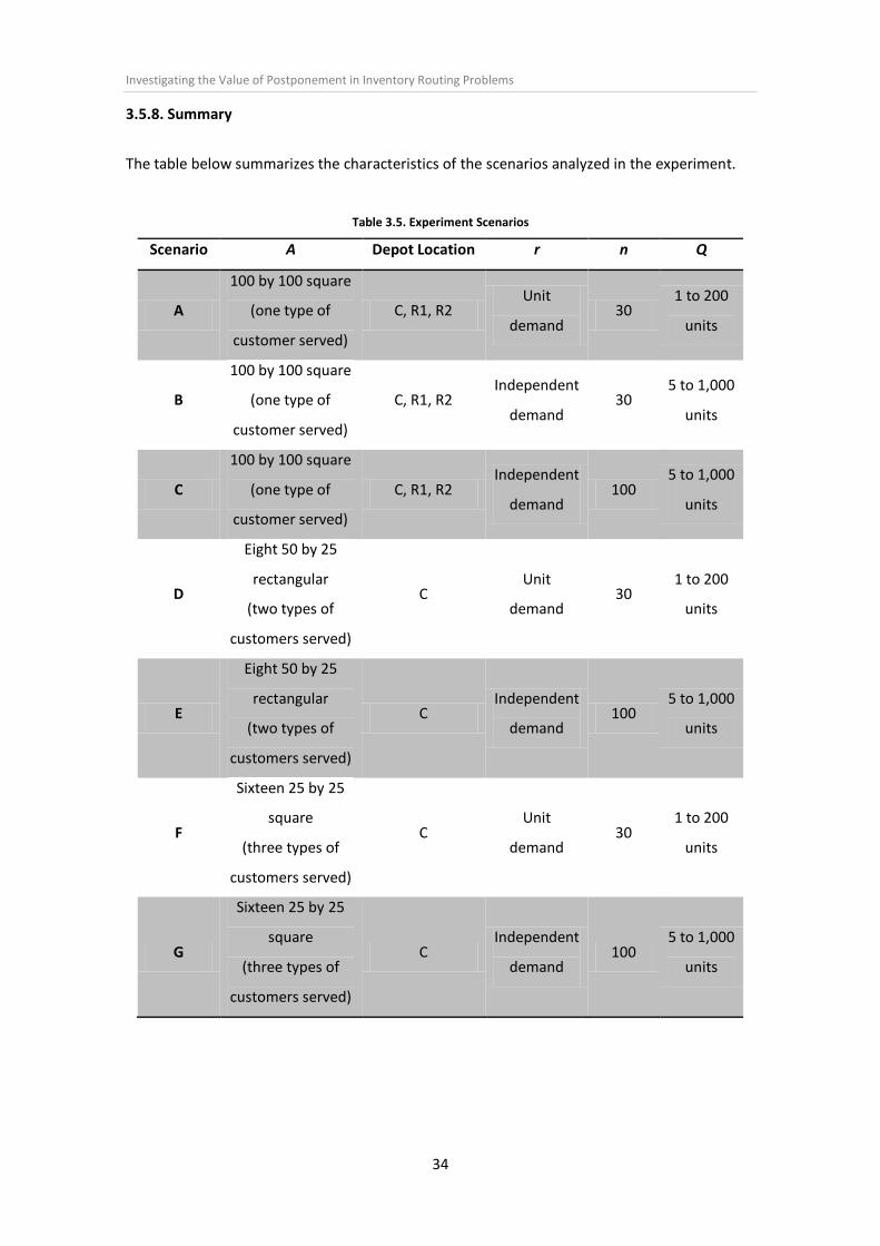
3.5.8. Summary
The table below summarizes the characteristics of the scenarios analyzed in the experiment.
Table 3.5. Experiment Scenarios
Scenario A Depot Location r n Q
A
100 by 100 square
(one type of
customer served)
C, R1, R2 Unit
demand 30
1 to 200
units
B
100 by 100 square
(one type of
customer served)
C, R1, R2 Independent
demand 30
5 to 1,000
units
C
100 by 100 square
(one type of
customer served)
C, R1, R2 Independent
demand 100
5 to 1,000
units
D
Eight 50 by 25
rectangular
(two types of
customers served)
C Unit
demand 30
1 to 200
units
E
Eight 50 by 25
rectangular
(two types of
customers served)
C Independent
demand 100
5 to 1,000
units
F
Sixteen 25 by 25
square
(three types of
customers served)
C Unit
demand 30
1 to 200
units
G
Sixteen 25 by 25
square
(three types of
customers served)
C Independent
demand 100
5 to 1,000
units

Investigating the Value of Postponement in Inventory Routing Problems
35
4. EXPERIMENT RESULTS
Before evaluating the impact of the experiment parameters, a detailed analysis of the
scenarios is presented with the corresponding results. Besides, the method applied
(continuous approximation theory) is explained in detail so that is simple to understand the
final outcomes. Yet, the diagrams are shown at the end of this chapter in order to focus in the
objective that is to find the optimal level of postponement in the diverse inventory routing
instances created.
The continuous approximation formula to calculate the total costs is,
2
)(2 max
maxmax
nrt
t
Anq
tq
nl
Q = Vehicle capacity (units)
n = Customers density
r = Customers demand rate (units)
q = Q/r = Average number of customers served per vehicle route
n/q = Number of trips required (rounded to the next integer)
l = Average line-haul distance
tmax = Maximum accumulation time (periods)
A = Size of the service area (distance units)
α = ratio between inventory holding costs and routing costs
)(q = Constant depending on the Euclidean metric and q
For example in scenario A (C), the total cost for α = 0.01 and tmax = 1 is,
74.295,2$01.02
30110
11
302597858226.382($)
CostTotal
All the values calculated for each scenario are displayed in the appendices.
Radial Routing Cost
Local Routing Cost
Inventory Holding Cost

Investigating the Value of Postponement in Inventory Routing Problems
36
4.1. Scenario A Results
The method to find the optimal level of postponement starts by computing the routing costs in
the environment created. In view of the fact that demand rate is unitary, the routing costs are
calculated by plugging the different values of the line-haul distances and the parameters into
the radial routing cost formula. For this scenario, the routing costs for each location of the
depot under max-postponement are revealed in figure 4.1.
INSERT FIGURE 4.1. ABOUT HERE
Meanwhile the vehicle capacity (or tmax) increases, the routing costs are minimized as well as
the number of trips required to serve all the customers. Notice also that for larger Q, the gap
between the C, R1 and R2 curves is shorter. This means that for large Q, a change in the
location of the depot will have a lower impact in the routing costs.
Even though postponement is generally minimizing routing costs (for detailed overview see
Muyldermans and Pang, 2009), inventory holding costs might increase. Therefore, an inventory
holding cost matrix as function of tmax and α is plotted resulting in the subsequent surface
graph.
INSERT FIGURE 4.2. ABOUT HERE
This figure shows that for large Q, the inventory holding costs increase. So a diagram of the
total costs is necessary to find the optimal postponement horizon, in which the routing costs
and inventory holding costs are reduced.
For this scenario, three surface graphs are plotted in order to determine the optimal
accumulation time for the different depot locations in function of α. The total cost surface
graphs for C, R1 and R2 configurations of the depot are,
INSERT FIGURE 4.3. ABOUT HERE
From the graphs, for higher α value the total costs increases in the meantime the vehicle
capacities (or tmax) are also increasing. In contrast, for lower α, the total costs decrease while Q
is increasing.

Investigating the Value of Postponement in Inventory Routing Problems
37
Total cost surface graph provides the information necessary to identify the optimal level of
postponement for the different values of α. Furthermore, this type of diagram also determines
the optimal vehicle capacity. For example in figure 4.3. (C), for α = 5, the minimum cost is
$829.7 which corresponds to a maximum accumulation time of 6 periods and a vehicle
capacity of 6 units.
For unit demand instances where the service area is divided, the total cost surface graph is
highly recommended to determine the optimal postponement horizons. Alternatively, as
scenario A has a unit demand rate with no service division, tmax as a function of α is calculated
by the following formula.
lt 2max
In fact, this expression is more accurate for this kind of instances because the first derivative of
the total cost function is taken. Then, the results for scenario A are presented in the optimal
postponement horizon curves.
INSERT FIGURE 4.4. ABOUT HERE
Basically, larger postponement horizons and bigger vehicle capacities should be used for the
R2 configuration of the depot. Besides, for α values in which ch >>> cr (holding cost dominates
routing cost), the optimal level of postponement must be smaller (short periods of time
between deliveries) in order to avoid higher holding costs at the customers. On the other
hand, for α values in which cr >>> ch (routing cost dominates holding cost); the maximum time
between deliveries should be longer to minimize the routing costs.
Table 4.1. shows the minimum possible costs ($), both optimal tmax (periods) and Q (units)
according to α and depot location employed in this scenario.

Investigating the Value of Postponement in Inventory Routing Problems
38
Table 4.1. Optimal Results for Scenario A
C R1 R2
α Cost tmax Q Cost tmax Q Cost tmax Q
0.01 37.11 124 124 52.49 175 175 62.08 207 207
0.05 82.99 55 55 117.36 78 78 138.81 93 93
0.1 117.36 39 39 165.97 55 55 196.31 65 65
0.25 185.56 25 25 262.43 35 35 310.39 41 41
0.5 262.43 17 17 371.13 25 25 438.95 29 29
0.75 321.41 14 14 454.54 20 20 537.61 24 24
1 371.13 12 12 524.85 17 17 620.77 21 21
2 524.85 9 9 742.25 12 12 877.91 15 15
3 642.81 7 7 909.07 10 10 1,075.21 12 12
5 829.87 6 6 1,173.61 8 8 1,388.09 9 9
10 1,173.71 4 4 1,659.73 6 6 1,963.06 7 7
4.2. Scenario B Results
Differing from scenario A, this instance involves radial and local routing costs. The total routing
costs for C, R1 and R2 can be observed in figure 4.5.
INSERT FIGURE 4.5. ABOUT HERE
Given that vehicles are travelling between customers (local routing), the radial routing costs
are minimized as there is no need to return to the depot until the entire load in the vehicle is
empty. Indeed, this reduction on the radial routing costs is higher than the costs incurred for
local routing; hence a reduction in the total routing costs is achieved.
On the contrary, the inventory holding costs for longer postponement horizons are greater
than those obtained in scenario A. The demand rate is the reason for this increase as the
customers are holding more units.
INSERT FIGURE 4.6. ABOUT HERE
For this scenario, the inventory holding costs dominates the routing costs. Thus, the total costs
are also greater for longer accumulation times than the calculated for scenario A. Total cost
surface graphs for C, R1 and R2 configurations of the depot are shown below.

Investigating the Value of Postponement in Inventory Routing Problems
39
INSERT FIGURE 4.7. ABOUT HERE
The same as in scenario A, for high α values and large postponement horizons, the total costs
for each configuration are bigger. In contrast, for low values of α and larger tmax the costs
decrease considerably. This observation remains constant over all the scenarios analyzed.
Therefore, a preliminary conclusion is that for instances where ch >>> cr , postponement
horizons should be shorter than for instances where cr >>> ch.
From the total cost surface graphs the minimum costs for each α value were determined by
extending the calculations. This means that an iterative analysis (over postponement horizons)
was performed in order to find the minimum costs. For example for a centrally located depot
with α = 0.01, the minimum cost was located between 50 periods and 70 periods. Afterwards,
calculating for each period (within the range) the total cost, the minimum was found in the
period 62 with a value of $56.56. The optimal postponement horizon curves for scenario B are
given in the following figure.
INSERT FIGURE 4.8. ABOUT HERE
Taking in consideration the procedure explained above, the minimum costs, optimal tmax and Q
(5*tmax) for the different depot locations are expressed in table 4.2.
Table 4.2. Optimal Results for Scenario B
C R1 R2
α Cost tmax Q Cost tmax Q Cost tmax Q
0.01 56.56 62 310 75.35 84 420 85.42 95 475
0.05 126.47 28 140 168.51 37 185 191.01 42 210
0.1 178.86 20 100 238.33 26 130 270.12 30 150
0.25 282.96 13 65 376.81 17 85 427.09 19 95
0.5 399.97 9 45 532.88 12 60 604.31 13 65
0.75 490.13 7 35 652.95 10 50 739.75 11 55
1 566.20 6 30 754.32 8 40 855.35 10 50
2 804.30 4 20 1,065.76 6 30 1,209.08 7 35
3 984.30 4 20 1,305.91 5 25 1,485.59 6 30
5 1,267.40 3 15 1,688.64 4 20 1,913.38 4 20
10 1,788.59 2 10 2,401.51 3 15 2,701.18 3 15

Investigating the Value of Postponement in Inventory Routing Problems
40
4.3. Scenario C Results
Modifying the population size of scenario B from 30 to 100 customers will have an impact in
the total costs. This can be explained immediately before analysing the problem regarding the
definitions of local routing cost and inventory holding cost. For higher population sizes, the
distance traversed by vehicles between customers will increase and so forth the routing costs.
On the other hand, more customers create more demand of goods, hence higher costs of
storage.
The analysis provides the following results.
Table 4.3. Optimal Results for Scenario C
C R1 R2
α Cost tmax Q Cost tmax Q Cost tmax Q
0.01 178.69 60 300 243.87 81 405 281.54 94 470
0.05 399.58 27 135 545.34 36 180 629.53 42 210
0.1 565.06 19 95 771.24 26 130 890.35 30 150
0.25 893.43 12 60 1,219.52 16 80 1,407.78 19 95
0.5 1,265.15 8 40 1,726.03 12 60 1,991.18 13 65
0.75 1,547.67 7 35 2,113.87 9 45 2,438.44 11 55
1 1,786.86 6 30 2,439.04 8 40 2,817.82 9 45
2 2,530.29 4 20 3,452.06 6 30 3,987.19 7 35
3 3,123.72 3 15 4,232.47 5 25 4,892.07 5 25
5 4,023.72 3 15 5,478.09 4 20 6,302.59 4 20
10 5,660.59 2 10 7,804.12 3 15 8,903.45 3 15
Results confirmed that for every value of α, the total costs are higher than those calculated for
scenario B. For example for α = 1, the total cost for a centrally located depot in scenario B is
$566.2. On the contrary, in scenario C is $1,786.86. Furthermore, the optimal values for tmax
and Q varied in low proportions.
4.4. Scenario D Results
The analysis of this scenario involves the evaluation of the total costs and postponement
horizons for a centrally located depot with service division. In the first place, the four areas
next to the depot are named S1, while the four located in the corners are called S2 (see figure
3.5.). Secondly, assuming that customers are homogeneously distributed over the entire

Investigating the Value of Postponement in Inventory Routing Problems
41
region, each sub-area has n/8 customers (in this case, 3.75 customers) due to symmetry.
Afterwards, given that demand rate is unitary; the routing costs calculated for one S1 and one
S2 are revealed in the following curves.
INSERT FIGURE 4.13. ABOUT HERE
The routing costs for serving customers located in S1 region are lower than the costs for the S2
region. However, the breach between the curves is relatively short because of the small
population size employed in this scenario.
Adding together the inventory holding costs (figure 4.14. reveals the inventory holding costs
for scenario D) with these values, the total costs are determined. Following figures represents
the total costs for S1 and S2 regions.
INSERT FIGURE 4.15. ABOUT HERE
Both graphs corroborate that for higher α and tmax values the total costs increases, while for
lower α and larger tmax the total costs decreases. To find the optimal trade-off between
inventory holding costs and routing costs the iterative procedure used for scenarios B and C is
applied. Then, the optimal postponement horizons for scenario D are,
INSERT FIGURE 4.16. ABOUT HERE
The graph shows that for every value of α, longer postponement horizons and bigger vehicle
capacities should be used to fulfill the customers’ requirements located in S2 region. Then, the
optimal Q, tmax and costs for S1 and S2 regions are shown in table 4.4.

Investigating the Value of Postponement in Inventory Routing Problems
42
Table 4.4. Optimal Results for Scenario D
S1 S2
α Cost tmax Q Cost tmax Q
0.01 2.11 56 56 2.66 65 65
0.05 4.72 25 25 5.93 32 32
0.1 6.67 18 18 8.38 22 22
0.25 10.55 11 11 13.26 14 14
0.5 14.92 8 8 18.75 10 10
0.75 18.32 7 7 22.96 8 8
1 21.14 6 6 26.51 7 7
2 29.83 4 4 37.49 5 5
3 37.33 4 4 45.93 4 4
5 52.33 4 4 60.93 4 4
10 89.83 4 4 98.43 4 4
The optimal costs calculated correspond to one S1 and one S2. Consequently, the total cost for
a centrally located depot with this type of service division is given by, Total Cost = 4*S1COST +
4*S2COST.
As a result, the optimal total costs (for each α) for scenario D are,
Table 4.5. Optimal Total Cost for Scenario D
α Cost (C)
0.01 19.08
0.05 42.6
0.1 60.2
0.25 95.24
0.5 134.68
0.75 165.12
1 190.6
2 269.28
3 333.04
5 453.04
10 753.04

Investigating the Value of Postponement in Inventory Routing Problems
43
4.5. Scenario E Results
Maintaining the service region divided into S1 and S2, and varying the population size to 100
customers (12.5 customers for each sub-area) with an independent demand rate, the optimal
tmax, Q (5* tmax) and costs for each α vary. This variation is presented in table 4.6.
Table 4.6. Optimal Results for Scenario E
S1 S2
α Cost tmax Q Cost tmax Q
0.01 20.60 55 275 25.11 67 335
0.05 47.04 20 100 56.16 30 150
0.1 65.16 17 85 79.42 21 105
0.25 103.00 11 55 125.63 13 65
0.5 145.73 8 40 177.82 9 45
0.75 178.68 6 30 217.62 8 40
1 206.81 6 30 251.39 7 35
2 291.46 4 20 355.69 5 25
3 357.36 3 15 435.24 4 20
5 469.86 3 15 561.58 3 15
10 657.92 2 10 795.49 2 10
Evaluating these results in comparison with the ones obtained in scenario D, it is possible to
state that for any α values, shorter periods of time between two deliveries should be
performed for an independent demand rate. For example for α = 0.01, the optimal
postponement horizon in scenario D (S1) is 56 periods while in scenario E (S1) is 55 periods.
Moreover, for independent demand rates bigger vehicle capacities are required in order to
satisfy the customers demand.
Following curves shows the optimal postponement horizon for scenario E.
INSERT FIGURE 4.20 ABOUT HERE
Notice that these values correspond for one S1 region and one S2 region. Afterwards, the total
cost for a centrally located depot is computed by using the same formula given to calculate the
total costs in scenario D. The values are expressed in table 4.7.

Investigating the Value of Postponement in Inventory Routing Problems
44
Table 4.7. Optimal Total Cost for Scenario E
α Cost (C)
0.01 182.84
0.05 412.80
0.1 578.32
0.25 914.52
0.5 1,294.20
0.75 1,585.20
1 1,832.80
2 2,588.60
3 3,170.40
5 4,125.76
10 5,813.64
Due to the independent demand rate applied in this scenario, the total costs are higher in
comparison with the total costs calculated for scenario D.
4.6. Scenario F Results
In contrast with scenarios D and E, the service region in this instance is divided into sixteen
smaller service areas, representing three different service rates. S1, S2 and S3 configurations
have the same amount of customers due to symmetry (see figure 3.6.). Therefore, as the
customers’ density is 30, each sub-area has 1.875 customers for mathematical analysis.
INSERT FIGURE 4.21. ABOUT HERE
The routing costs incurred for serving customers located in S3 are higher than the computed
for the other two regions. Appreciate that in the meantime the vehicle capacity or the
maximum accumulation time increases the gap between the curves decreases. This means that
for higher Q or tmax, the routing costs become similar for the reason that fewer trips are
required to serve the customers distributed within the different service areas. Applying then
the methodology used in scenarios B, C, D and E; the total costs for scenario F are expressed in
the following surface diagrams.
INSERT FIGURE 4.23. ABOUT HERE

Investigating the Value of Postponement in Inventory Routing Problems
45
From the graphs it can be determined that for S3 region, the total costs are bigger and the
optimal postponement horizons are larger.
INSERT FIGURE 4.24. ABOUT HERE
The optimal accumulation times, vehicle capacities and minimum costs in function of α for
each sub-region are given in table 4.8.
Table 4.8. Optimal Results for Scenario F
S1 S2 S3
α Cost tmax Q Cost tmax Q Cost tmax Q
0.01 1.20 64 64 1.74 93 93 2.00 107 107
0.05 2.68 29 29 3.88 41 41 4.48 48 48
0.1 3.79 20 20 5.53 26 26 6.34 34 34
0.25 5.99 13 13 8.68 19 19 10.02 21 21
0.5 8.47 9 9 12.28 13 13 14.17 15 15
0.75 10.39 7 7 15.04 11 11 17.36 12 12
1 12.00 6 6 17.37 9 9 20.04 11 11
2 17.03 5 5 24.61 7 7 28.38 8 8
3 20.81 4 4 30.14 5 5 34.72 6 6
5 26.82 3 3 38.85 4 4 44.85 5 5
10 37.88 2 2 54.92 3 3 132.78 3 3
To obtain the total costs for the entire region, the expression Total Cost = 4*S1COST + 8*S2COST +
4*S3COST, is used. Thus, the optimal total costs (for each α) for scenario F are shown in table
4.9.
Table 4.9. Optimal Total Cost for Scenario F
α Cost (C)
0.01 26.70
0.05 59.70
0.1 84.73
0.25 133.51
0.5 188.77
0.75 231.32
1 267.14
2 378.50
3 463.24
5 597.42
10 1,122.00

Investigating the Value of Postponement in Inventory Routing Problems
46
4.7. Scenario G Results
Maintaining the service region divided into S1, S2 and S3, and varying the population size to
100 customers (6.25 customers for each sub-region) with an independent demand rate, the
optimal vehicle capacities (5*tmax), tmax and costs in function of α for scenario G are expressed
in table 4.10.
Table 4.10. Optimal Results for Scenario G
S1 S2 S3
α Cost tmax Q Cost tmax Q Cost tmax Q
0.01 8.63 46 230 11.73 63 315 13.33 71 355
0.05 19.30 21 105 26.24 28 140 29.81 32 160
0.1 27.31 14 70 37.11 20 100 42.16 22 110
0.25 43.17 9 45 58.71 13 65 66.66 14 70
0.5 61.19 7 35 82.98 9 45 94.26 10 50
0.75 74.89 5 25 101.67 7 35 115.48 8 40
1 86.61 5 25 117.45 6 30 133.31 7 35
2 122.47 3 15 166.79 4 20 188.51 5 25
3 150.60 3 15 204.29 4 20 230.95 4 20
5 193.08 2 10 263.02 3 15 298.56 3 15
10 286.83 2 10 371.09 2 10 424.40 2 10
The same conclusion arises observing the results for scenario G. For far away service areas,
vehicle capacities should be bigger and postponement horizons must be larger in order to
obtain the minimum possible costs. Additionally, optimal accumulation times decrease while
the inventory holding costs become more important. This can be recognized in the following
figure.
INSERT FIGURE 4.28. ABOUT HERE
Finally, to determine the optimal costs for a centrally located depot with three different
service rates, the formula given for scenario F is applied. Then, the optimal total costs for each
value of α are given in table 4.11.

Investigating the Value of Postponement in Inventory Routing Problems
47
Table 4.11. Optimal Total Cost for Scenario G
α Cost (C)
0.01 181.72
0.05 406.35
0.1 574.74
0.25 909.00
0.5 1,285.67
0.75 1,574.83
1 1,819.24
2 2,578.27
3 3,160.53
5 4,070.69
10 5,813.63
4.8. Summary
This section summarizes in three different tables the results obtained in the experiment.
Furthermore, a brief analysis of the results is presented in function of the trade-offs between
routing and inventory holding costs studied (α).
In the first place, table 4.12. displays the optimal postponement horizons calculated for the
different inventory routing instances created.
Table 4.12. Optimal Postponement Horizons (Periods)

Investigating the Value of Postponement in Inventory Routing Problems
48
For the scenarios analyzed, the optimal level of postponement haves a similar behaviour
according to the values of α. On one hand, when ch >>> cr; tmax trends to be lower. This means
that for high α values, the time accumulated between deliveries must be shorter in order to
avoid high costs of storage. On the contrary, when cr >>> ch; optimal postponement horizons
are larger due to the high transportation costs.
It is important to mention that every scenario studied requires postponement in order to
reduce the overall costs. Consequently, it is possible to state that postponement is a strategy
that helps to minimize the total costs in inventory routing problems.
In the second place, table 4.13. presents the optimal vehicle capacities for each of the
experiments instances developed.
Table 4.13. Optimal Vehicle Capacities (Units)
Notice that the effect of α described previously for the optimal accumulation time is the same
for the vehicle capacities. Therefore, for high values of α, smaller Q are required while for low
values of α, bigger vehicle capacities are necessary.

Investigating the Value of Postponement in Inventory Routing Problems
49
Finally, table 4.14. shows the minimum total costs in function of α for the diverse routing
scenarios analyzed.
Table 4.14. Minimum Total Costs ($)
In contrast with tmax and Q, for high α values the total costs trends to increase while for low α
values the total costs decrease. This means that under a maximum postponement strategy, the
total costs increases meanwhile holding costs become more significant.

Investigating the Value of Postponement in Inventory Routing Problems
50
4.9. Figures
Figure 4.1. Scenario A – Routing Cost Curves
Figure 4.2. Scenario A – Inventory Holding Cost Surface Graph
0
1000
2000
3000
4000
5000
6000
7000
1 3 6 15 40 60 80 150
Ro
uti
ng
Co
st
Q = tmax
Scenario A Routing Cost Curves
C
R1
R2
0,01
0,5
30
10000
20000
30000
1
515
5080 200Alpha
Inve
nto
ry
Ho
ldin
g C
ost
Q = tmax
Scenario AInventory Holding Cost Surface Graph

Investigating the Value of Postponement in Inventory Routing Problems
51
Figure 4.3. Scenario A – Total Cost Graphs
0,01
0,5
30
10000
20000
30000
1
515
5080
200
Alpha
Tota
l Co
st
Q = tmax
Scenario ATotal Cost Surface Graph (C)
0,01
0,5
30
10000
20000
30000
1
515
5080
200Alpha
Tota
l Co
st
Q = tmax
Scenario ATotal Cost Surface Graph (R1)
0,01
0,5
30
10000
20000
30000
1
515
5080
200Alpha
Tota
l Co
st
Q = tmax
Scenario ATotal Cost Surface Graph (R2)
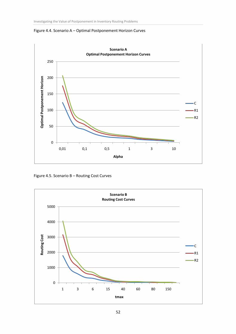
Investigating the Value of Postponement in Inventory Routing Problems
52
Figure 4.4. Scenario A – Optimal Postponement Horizon Curves
Figure 4.5. Scenario B – Routing Cost Curves
0
50
100
150
200
250
0,01 0,1 0,5 1 3 10
Op
tim
al P
ost
po
nem
ent
Ho
rizo
n
Alpha
Scenario AOptimal Postponement Horizon Curves
C
R1
R2
0
1000
2000
3000
4000
5000
1 3 6 15 40 60 80 150
Ro
uti
ng
Co
st
tmax
Scenario B Routing Cost Curves
C
R1
R2

Investigating the Value of Postponement in Inventory Routing Problems
53
Figure 4.6. Scenario B – Inventory Holding Cost Surface Graph
Figure 4.7. Scenario B – Total Cost Surface Graphs
0,01
0,5
30
30000
60000
90000
1
515
5080
200Alpha
Inve
nto
ry
Ho
ldin
g C
ost
tmax
Scenario BInventory Holding Cost Surface Graph
0,01
0,5
30
30000
60000
90000
1
515
5080
200Alpha
Tota
l Co
st
tmax
Scenario B Total Cost Surface Graph (C)
0,01
0,5
30
30000
60000
90000
1
515
5080
200Alpha
Tota
l Co
st
tmax
Scenario B Total Cost Surface Graph (R1)

Investigating the Value of Postponement in Inventory Routing Problems
54
Figure 4.8. Scenario B – Optimal Postponement Horizon Curves
0,01
0,5
30
30000
60000
90000
1
515
5080
200Alpha
Tota
l Co
st
tmax
Scenario BTotal Cost Surface Graph (R2)
0
10
20
30
40
50
60
70
80
90
100
0,01 0,1 0,5 1 3 10
Op
tim
al P
ost
po
nem
ent
Ho
rizo
n
Alpha
Scenario BOptimal Postponement Horizon Curves
C
R1
R2

Investigating the Value of Postponement in Inventory Routing Problems
55
Figure 4.9. Scenario C – Routing Cost Curves
Figure 4.10 Scenario C – Inventory Holding Cost Surface Graph
0
2000
4000
6000
8000
10000
12000
14000
16000
1 3 6 15 40 60 80 150
Ro
uti
ng
Co
st
tmax
Scenario CRouting Cost Curves
C
R1
R2
0,01
0,5
30
100000
200000
300000
1
515
5080 200
Alpha
Inve
nto
ry
Ho
ldin
g C
ost
tmax
Scenario CInventory Holding Cost Surface Graph

Investigating the Value of Postponement in Inventory Routing Problems
56
Figure 4.11. Scenario C – Total Cost Surface Graphs
0,01
0,5
30
100000
200000
300000
1
515
5080
200Alpha
Tota
l Co
st
tmax
Scenario C Total Cost Surface Graph (C)
0,01
0,5
30
100000
200000
300000
1
515
5080
200
Alpha
To
tal C
ost
tmax
Scenario CTotal Cost Surface Graph (R1)
0,01
0,5
30
100000
200000
300000
1
515
5080
200Alpha
Tota
l Co
st
tmax
Scenario CTotal Cost Surface Graph (R2)

Investigating the Value of Postponement in Inventory Routing Problems
57
Figure 4.12. Scenario C – Optimal Postponement Horizon Curves
Figure 4.13. Scenario D – Routing Cost Curves
0
10
20
30
40
50
60
70
80
90
100
0,01 0,1 0,5 1 3 10
Op
tim
al P
ost
po
nem
ent
Ho
rizo
n
Alpha
Scenario C Optimal Postponement Horizon Curves
C
R1
R2
0
50
100
150
200
250
300
350
400
1 3 6 15 40 60 80 150
Ro
uti
ng
Co
st
Q = tmax
Scenario DRouting Cost Curves
S1
S2

Investigating the Value of Postponement in Inventory Routing Problems
58
Figure 4.14. Scenario D – Inventory Holding Cost Surface Graph
Figure 4.15. Scenario D – Total Cost Surface Graphs
0,01
0,5
30
1000
2000
3000
4000
1
515
5080
200Alpha
Inve
nto
ry
Ho
ldin
g C
ost
Q = tmax
Scenario DInventory Holding Cost Surface Graph
0,01
0,5
30
1000
2000
3000
4000
1
515
5080
200Alpha
Tota
l Co
st
Q = tmax
Scenario DTotal Cost Surface Graph (S1)
0,01
0,5
30
1000
2000
3000
4000
1
515
5080
200Alpha
Tota
l Co
st
Q = tmax
Scenario D Total Cost Surface Graph (S2)

Investigating the Value of Postponement in Inventory Routing Problems
59
Figure 4.16. Scenario D – Optimal Postponement Horizon Curves
Figure 4.17. Scenario E – Routing Cost Curves
0
10
20
30
40
50
60
70
0,01 0,1 0,5 1 3 10
Op
tim
al P
ost
po
nem
ent
Ho
rizo
n
Alpha
Scenario DOptimal Postponement Horizon Curves
S1
S2
0
100
200
300
400
500
600
700
800
900
1 3 6 15 40 60 80 150
Ro
uti
ng
Co
st
tmax
Scenario ERouting Cost Curves
S1
S2

Investigating the Value of Postponement in Inventory Routing Problems
60
Figure 4.18. Scenario E – Inventory Holding Cost Surface Graph
Figure 4.19. Scenario E – Total Cost Surface Graphs
0,01
0,5
30
10000200003000040000
1
515
5080 200
Alpha
Inve
nto
ryH
old
ing
Co
st
tmax
Scenario EInventory Holding Cost Surface Graph
0,01
0,5
30
100002000030000
40000
13
615
40 60 80 150Alpha
Tota
l Co
st
tmax
Scenario ETotal Cost Surface Graph (S1)
0,01
0,5
30
10000200003000040000
13
615
40 60 80 150Alpha
Tota
l Co
st
tmax
Scenario ETotal Cost Surface Graph (S2)

Investigating the Value of Postponement in Inventory Routing Problems
61
Figure 4.20. Scenario E – Optimal Postponement Horizon Curves
Figure 4.21. Scenario F – Routing Cost Curves
0
10
20
30
40
50
60
70
80
0,01 0,1 0,5 1 3 10
Op
tim
al P
ost
po
nem
ent
Ho
rizo
n
Alpha
Scenario EOptimal Postponement Horizon Curves
S1
S2
0
50
100
150
200
250
1 3 6 15 40 60 80 150
Ro
uti
ng
Co
st
Q = tmax
Scenario FRouting Cost Curves
S1
S2
S3

Investigating the Value of Postponement in Inventory Routing Problems
62
Figure 4.22. Scenario F – Inventory Holding Cost Surface Graph
Figure 4.23. Scenario F – Total Cost Surface Graphs
0,01
0,5
30
500
1000
1500
2000
1
515
5080
200Alpha
Inve
nto
ry
Ho
ldin
g C
ost
Q = tmax
Scenario FInventory Holding Cost Surface Graph
0,01
0,5
30
500
1000
1500
2000
1
515
5080
200Alpha
Tota
l Co
st
Q = tmax
Scenario FTotal Cost Surface Graph (S1)
0,01
0,5
30
500
1000
1500
2000
1
515
5080
200Alpha
Tota
l Co
st
Q = tmax
Scenario FTotal Cost Surface Graph (S2)

Investigating the Value of Postponement in Inventory Routing Problems
63
Figure 4.24. Scenario F – Optimal Postponement Horizon Curves
0,01
0,5
30
500
1000
1500
2000
1
515
5080
200Alpha
Tota
l Co
st
Q = tmax
Scenario FTotal Cost Surface Graph (S3)
0
20
40
60
80
100
120
0,01 0,1 0,5 1 3 10
Op
tim
al P
ost
po
nem
ent
Ho
rizo
n
Alpha
Scenario FOptimal Postponement Horizon Curves
S1
S2
S3

Investigating the Value of Postponement in Inventory Routing Problems
64
Figure 4.25. Scenario G – Routing Cost Curves
Figure 4.26. Scenario G – Inventory Holding Cost Surface Graph
0
50
100
150
200
250
300
350
400
450
500
1 3 6 15 40 60 80 150
Ro
uti
ng
Co
st
tmax
Scenario GRouting Cost Curves
S1
S2
S3
0,01
0,5
30
5000
10000
15000
20000
1
515
5080 200
Alpha
Inve
nto
ry
Ho
ldin
g C
ost
tmax
Scenario GInventory Holding Cost Surface Graph

Investigating the Value of Postponement in Inventory Routing Problems
65
Figure 4.27. Scenario G – Total Cost Surface Graphs
0,01
0,5
30
5000
10000
15000
20000
1
515
5080
200Alpha
Tota
l Co
st
tmax
Scenario GTotal Cost Surface Graph (S1)
0,01
0,5
30
5000
10000
15000
20000
1
515
5080
200Alpha
Tota
l Co
st
tmax
Scenario GTotal Cost Surface Graph (S2)
0,01
0,5
30
5000
10000
15000
20000
1
515
5080
200Alpha
Tota
l Co
st
tmax
Scenario GTotal Cost Surface Graph (S3)

Investigating the Value of Postponement in Inventory Routing Problems
66
Figure 4.28. Scenario G – Optimal Postponement Horizon Curves
0
10
20
30
40
50
60
70
80
0,01 0,1 0,5 1 3 10
Op
tim
al P
ost
po
ne
me
nt
Ho
rizo
n
Alpha
Scenario GOptimal Postponement Horizon Curves
S1
S2
S3

Investigating the Value of Postponement in Inventory Routing Problems
67
5. EXPERIMENT DISCUSSION
The optimal accumulation times in which inventory holding costs and routing costs are
minimized is also affected by the diverse parameters analyzed in the experiment. The first
conclusion is that the vehicle capacities are directly proportional to the optimal postponement
horizons. i.e., bigger vehicle capacities are required for higher postponement horizons and vice
versa for small Q. Furthermore, other parameters such as the service region (A), the depot
location, customers demand rate (r) and customers’ density (n) have different impacts over the
optimal postponement horizons and inventory routing costs. Hence, this chapter provides
insight of the parameters impact over the optimal values for tmax and IRP costs.
5.1. Service Region (A) Impact
Concerning a centrally located depot, three different configurations for A were analyzed to see
the impact of splitting the service region in inventory routing problems. In the first place the
service region for scenarios A, B and C was a 100 by 100 square area having a single service
frequency. Secondly, the service region for scenarios D and E was divided into eight 50 by 25
rectangular areas having two service rates represented in the regions S1 and S2. Finally, the
service region for scenarios F and G was divided into sixteen 25 by 25 square areas having
three service frequencies denoted in the regions S1, S2 and S3.
From the results, it can be concluded that the optimal level of postponement (for the cases in
which the service region is divided) is higher for those areas located far away from the depot.
In other words, taking in consideration the service region used for scenarios D and E,
customers located in S2 areas should be served in larger postponement horizons than
customers in S1 areas (see figures 4.16. and 4.20.) in order to obtain the minimum possible
costs. Moreover, for remote areas the total costs are higher since the average line-haul
distance is bigger and because higher holding costs at the customers are incurred (higher level
of postponement causes higher holding costs).
Splitting the service area also haves an impact over the total costs in the entire region.
Regarding a unit demand rate, the total costs are minimized when the service region is
partitioned. This is because the costs of storage at the customers are lower and also because
fewer tours are required to serve all the customers within the different service areas. For

Investigating the Value of Postponement in Inventory Routing Problems
68
example in scenario A (no service division) the total costs for α = 1 are $371.13, while for
scenario D and scenario F the total costs are $190.6 and $267.14 respectively. In fact, the
service division applied to scenario D is the best option to reduce the overall costs in a unit
demand rate with a centrally located depot. Following curves shows these observations.
Figure 5.1. Total Cost Curves for Scenarios A,D and F (C)
On the contrary, regarding an independent demand rate, the service division causes higher
costs. This effect can be explained by the bin packing trouble that is an important aspect in
inventory routing problems. Bin packing refers to the procedure in which items are packed into
bins.
In this dissertation, the bins are the vehicles and the items are the goods demanded by the
customers. Therefore, for independent demand rates since the variability of required goods is
higher, packing the items into the vehicles becomes more intricate. For example consider a
situation where the vehicle capacity is 14 units and five customers are ordering 3 units each
(total demand equal to 15 units). Obviously it is not possible to combine the 15 units in the
vehicle so only four of the customers are served in a single tour. This means that two tours are
required to satisfy the five customers and for this reason the radial routing costs increases for
each of the service areas causing an increase in the total costs for the entire region.
0
200
400
600
800
1000
1200
0.01 0.1 0.5 1 3 10
Tota
l Co
st
Alpha
Total Cost Curves forScenarios A, D and F (C)
Scenario A
Scenario D
Scenario F

Investigating the Value of Postponement in Inventory Routing Problems
69
The impact of splitting the service region under an independent demand rate was determined
by comparing the total costs of scenarios C, E and G. This comparison is shown in table 5.1.
Table 5.1. Minimum Total Cost for Scenarios C, E, and G (C)
α Scenario C Scenario E Scenario G
0.01 178.69 182.84 181.72
0.05 399.58 412.80 406.35
0.1 565.06 578.32 574.74
0.25 893.43 914.52 909.00
0.5 1,265.15 1,294.20 1,285.67
0.75 1,547.67 1,585.20 1,574.83
1 1,786.86 1,832.80 1,819.24
2 2,530.29 2,588.60 2,578.27
3 3,123.72 3,170.40 3,160.53
5 4,023.72 4,125.76 4,070.69
10 5,660.59 5,813.64 5,813.63
In this case, the difference in the total costs among the three scenarios is relatively short due
to the high number of customers contained in the service region (100 customers). However,
for smaller population sizes this difference increases for the reason that the radial routing
costs becomes more significant. Therefore, the best alternative for an independent demand
rate is the scenario with no service division (scenario C).
5.2. Depot Location Impact
In order to see the impact of depot location in inventory routing problems, three spatial
configurations were used: centrally, remote 1 and remote 2.
From the optimal postponement horizon curves plotted for scenarios A, B and C (see figures
4.4., 4.8. and 4.12. respectively) it is possible to conclude that the optimal time between two
customers visit must be larger for remote configurations of the depot and shorter for a
centrally located depot. This is explained by analyzing the importance of two routing costs: the
radial routing costs and the local routing costs. Clearly, radial routing costs are dominant in
remote configurations of the depot. So to reduce the total costs, fewer tours should be
performed by enlarging the postponement horizon. On the other hand, as local routing costs
are more important in a centrally located depot; smaller levels of postponement are required
in order to fulfill fewer customers on each tour.

Investigating the Value of Postponement in Inventory Routing Problems
70
Regarding the costs, the following table shows the minimum total costs for the three spatial
configurations of the depot in scenarios A, B and C.
Table 5.2. Minimum Total Costs for Scenarios A, B and C (C, R1 and R2)
From the table, is evidently that for remote configurations the total costs increases. This is
because for R1 and R2, the optimal postponement horizons are larger and thus the costs of
storage are greater. On the contrary for a centrally located depot, the costs are smaller as a
result of lower costs of storage.
5.3. Customers Demand Rate (r) Impact
In the scenarios created, two types of demand rates were applied. In the cases where the
customers demand rate is unitary, the optimal postponement horizons are larger given that
the routing cost involves only radial routing distances. i.e., routing costs are represented by the
distances travelled by the vehicle from the depot to the customers. On the contrary, for
independent demand instances, the accumulation times between two deliveries must be
shorter since bigger vehicle capacities are used and local routing is permitted. For example
taking in consideration scenarios A (unit) and B (independent) with a centrally located depot,
for α = 1 the optimal postponement horizon is 12 and 6 periods respectively. Likewise,
considering a R1 configuration, for α = 10 the optimal postponement horizon is 6 and 3 periods
respectively.

Investigating the Value of Postponement in Inventory Routing Problems
71
Analyzing the impact of the customers demand rate in the total costs, it is possible to mention
that unit demand instances showed an improvement over independent demand. This is due to
the fact that bin packing is more complicated in independent demand rates. Additionally, this
can be explained as a consequence of the high costs of storage that customers incurs by
holding more units when r = 3. Plotting the total costs for scenarios A and B as a function of α,
the improvement can be appreciated for each configuration of the depot.
Figure 5.2.Unit Demand (Scenario A) vs. Independent Demand (Scenario B)
Figure 5.2. also corroborates that for remote configurations of the depot the total costs are
higher.
5.4. Customers Density (n) Impact
Population sizes of 30 customers and 100 customers were studied in order to see the impact of
customers’ density in inventory routing problems. Comparing the results achieved in scenario
B with the results of scenario C, it is possible to conclude that a variation in the size of the
population will affect the total costs. i.e., bigger population sizes increases the total costs and
smaller population sizes decreases the total costs.
On the other hand, the optimal postponement horizon curves plotted for scenarios B and C
(see figures 4.8. and 4.12. respectively) revealed that the impact of the customers density in
the optimal accumulation time is low. For example in a centrally located depot, for α = 0.1 the
optimal postponement horizon in scenario B is 20 periods while in scenario C is 19 periods.
0
500
1000
1500
2000
2500
3000
0 2 4 6 8 10
To
tal C
ost
Alpha
Unit Demand (Scenario A) vs Independent Demand (Scenario B)
Scenario A (C)
Scenario B (C)
Scenario A (R1)
Scenario B (R1)
Scenario A (R2)
Scenario B (R2)

Investigating the Value of Postponement in Inventory Routing Problems
72
6. CONCLUSION
The aim of this dissertation was to find the optimal postponement horizon in which the routing
costs and the inventory holding costs of diverse routing scenarios were reduced. The study was
carried out by applying a continuous approximation model revealing that postponement is a
strategy that minimizes the total costs in inventory routing problems.
The research exposed that the optimal postponement horizon was principally influenced by
the ratio between the inventory holding costs and the routing costs (α). Moreover, important
impacts in the optimal accumulation time were due to changes in the experiment parameters
such as service region, depot location, customers demand rate and vehicle capacity.
In particular, the optimal level of postponement is unique for a defined combination of
problem parameters. Therefore, by analyzing the different scenarios created, key findings
about postponement in inventory routing problems were achieved. These findings can be
divided into two main categories. On one hand, the optimal postponement horizon is shorter
when,
The inventory holding costs dominates the routing costs (ch >>> cr).
The vehicle capacity decreases.
The depot is centrally located (i.e., the local routing cost dominates the radial routing
costs).
The customers are located in service areas near the depot.
The customers demand rate is independent (i.e., bin packing is more intricate).
On the other hand, optimal level of postponement is higher under reverse conditions. For
example when the vehicle capacity increases or when the depot is located in a remote
configuration.
Other objective of this research was to find the impact of the problem parameters in the total
costs in inventory routing problems. Therefore, the total costs in IRPs should be reduced when,
The customers are located in service areas near the depot.
The customers demand rate is unitary (i.e., bin packing is simple).

Investigating the Value of Postponement in Inventory Routing Problems
73
The customers’ density is lower.
The postponement level is higher and the vehicle capacity increases (for cases when
routing costs dominates the inventory holding costs).
The postponement level is lower and the vehicle capacity decreases (for cases when
inventory holding costs dominate the routing costs).
The depot is centrally located (i.e., the local routing cost dominates the radial routing
cost).
However, the total costs in IRPs increases in the opposite conditions.
Future extensions of this work could include comparing the results with a local search
procedure (Muyldermans and Pang, 2009) to verify the key findings about postponement in
IRPs. Furthermore, some additional criteria on the vehicle routes could be incorporated (pick-
up and delivery) or perhaps the square service region analyzed could be replaced by an
asymmetrical shape to see the impact of districting decisions in inventory routing problems.

Investigating the Value of Postponement in Inventory Routing Problems
74
7. REFERENCES
Allison L (1999), ‘Graphs’, Monash Univeristy, Australia.
Available at: http://www.csse.monash.edu.au/~lloyd/tildeAlgDS/Graph [Accessed on 26 July
2009].
Beullens P, Oudheusden D V and Wassenhove L N (2004), ‘Collection and vehicle routing
issues in reverse logistics’, In Dekker R, Fleischmann M, Inderfurth K and Wassenhove L N
(Eds.), Reverse Logistics: Quantitative Models for Closed-loop Supply Chains, Springer, pp. 95-
133.
Bodin L and Golden B (1981), ‘Classification in vehicle routing and scheduling’, Networks, Vol.
11, pp. 97-108.
Bodin L, Golden B, Assad A and Ball M (1983), ‘Routing and Scheduling of Vehicles and Crews:
The State of the Art’, International Journal of Computers and Operations Research, Vol. 10 (2),
pp. 63-211.
Campbell A, Clarke L, Kleywegt A and Savelsbergh M (1997), ‘The Inventory Routing Problem’,
Georgia Institute of Technology, Atlanta, GA.
Campbell J F (1993), ‘One-to-many distribution with transhipments: an analytic model’,
Transportation Science, Vol. 27, pp. 330-340.
Campbell J F (1996), ‘Continuous approximation models in freight distribution: An overview’,
Transportation Research, Part B: Methodological, Vol. 30 (3), pp. 163-188.
Chen S, Golden B and Wasil E (2007), ‘The split delivery vehicle routing problem: Applications,
algorithms, test problems, and computational results’, Networks, Vol. 49 (4), pp. 318-329.
Chen Y M and Lin C T (2009), ‘A coordinated approach to hedge the risks in stochastic
inventory-routing problem’, Computers & Industrial Engineering, Vol. 56 (3), pp. 1095-1112.

Investigating the Value of Postponement in Inventory Routing Problems
75
Clarke G and Wright J W (1964), ‘Scheduling of vehicles from a central depot to a number of
delivery points’, Operations Research, Vol. 12 (4), pp. 568-581.
Coene S, Arnout A and Spieksma F C R (2008), ‘The Periodic Vehicle Routing Problem: A Case
Study’, Katholieke Universiteit Leuven, Belgium.
Cordeau J F, Laporte G, Savelsbergh M P W and Vigo D (2007), ‘Vehicle Routing’,
Transportation, Vol. 14, pp. 367-384.
Crevier B, Cordeau J F and Laporte G (2007), ‘The multi-depot vehicle routing problem with
inter-depot routes’, European Journal of Operational Research, Vol. 176, pp. 756-773.
Daganzo C F (1984a), ‘The length of tours in zones of different shapes’, Transportation
Research, Part B: Vol. 18 (2), pp. 135-146.
Daganzo C F (1984b), ‘The distance travelled to visit N points with a maximum of C stops per
vehicle: an analytic model and an application’, Transportation Science, Vol. 18, pp. 331-350.
Daganzo C F (2005). Logistics systems analysis, (4th Edition). Springer-Verlag, Berlin, Heidelberg.
Francis P, Smilowitz K and Tzur M (2006), ‘The Periodic Vehicle Routing Problem with Service
Choice’, Transportation Science, Vol. 40 (4), pp. 439–454.
Gendreau M, Laporte G and Seguin R (1996), ‘Invited Review: Stochastic vehicle routing’,
European Journal of Operational Research, Vol. 88, pp. 3-12.
Golden B and Assad A (1988). Vehicle Routing: Methods and Studies. Studies in Management
Science and Systems. Maryland, U.S.A.
Guneri A F (2007), ‘Physical distribution activities and vehicle routing problems in logistics
management: a case study’, Proceedings of the Institution of Mechanical Engineers, Part B:
Journal of Engineering Manufacture, Vol. 221 (1), pp. 123-133.
Kjeldsen K H (2008), ‘Classification of routing and scheduling problems in liner shipping’,
Working paper, Aarhus University Business School, Denmark.

Investigating the Value of Postponement in Inventory Routing Problems
76
Kleywegt A J, Nori V S and Savelsbergh M W P (2000), ‘The Stochastic Inventory Routing
Problem with Direct Deliveries’, Transportation Science, Vol. 36, pp. 94-118.
Larsen A (2000), ‘The Dynamic Vehicle Routing Problem’, PhD Thesis, University of Denmark.
Moin N H and Salhi S (2007), ‘Inventory routing problems: a logistical overview’, Journal of the
Operational Research Society, Vol. 58, pp. 1185–1194.
Muyldermans L and Pang G (2009), ‘Vehicle routing and the value of postponement’,
Nottingham University Business School, UK.
Newell G F (1971), ‘Dispatching policies for a transportation route’, Transportation Science,
Vol. 5, pp. 91-105.
Ouyang Y (2007), ‘Design of vehicle routing zones for large-scale distribution systems’,
Transportation Research, Part B: Methodological, Vol. 41 (10), pp. 1079-1093.
Simchi-Levi D, Kaminsky P and Simchi-Levi E (2000). Designing and managing the supply chain:
Concepts, strategies, and case studies. Tata McGraw-Hill.
Toth P and Vigo D (2002). The Vehicle Routing Problem. SIAM monographs on discrete
mathematics and applications. Philadelphia, PA.
Woensel T, Kerbache L, Peremans H and Vandaele N (2008), ‘Vehicle routing with dynamic
travel times: A queueing approach’, Journal of Operational Research, Vol. 186 (3), pp. 990-
1007.

Investigating the Value of Postponement in Inventory Routing Problems
77
Web References
1. Massachusetts Institute of Technology:
http://web.mit.edu/
2. Vehicle Routing Problem Illustration:
http://upload.wikimedia.org/wikipedia/commons/thumb/9/94/Vrp_esquema.png/263
px-Vrp_esquema.png
3. Vehicle Routing Problem Web:
http://neo.lcc.uma.es/radi-aeb/WebVRP/
4. Vehicle Routing Problem with Pick-Up and Delivery Illustration:
http://www.hindawi.com/floats/697981/figures/697981.fig.002.jpg

Investigating the Value of Postponement in Inventory Routing Problems
78
8. APPENDICES
Appendix A: Scenario A
Values for Routing Cost Curves
Q = tmax C R1 R2
1 2,295.59 4,591.17 6,422.68
2 1,147.79 2,295.59 3,211.34
3 765.20 1,530.39 2,140.89
5 459.12 918.23 1,284.54
6 382.60 765.20 1,070.45
10 229.56 459.12 642.27
15 153.04 306.08 428.18
30 76.52 153.04 214.09
40 57.39 11.78 160.57
50 45.91 91,82 128.45
60 38.26 76.52 107.04
70 32.79 65.59 91.75
80 28.69 57.39 80.28
120 19.13 38.26 53.52
150 15.30 30.61 42.82
200 11.48 22.96 32.11
Values for Inventory Holding Cost Surface Graph
Q = tmax \ α 0.01 0.05 0.10 0.25 0.50 0.75 1.00 2.00 3.00 5.00 10.00
1 0.15 0.75 1.50 3.75 7.50 11.25 15.00 30.00 45.00 75.00 150.00
2 0.30 1.50 3.00 7.50 15.00 22.50 30.00 60.00 90.00 150.00 300.00
3 0.45 2.25 4.50 11.25 22.50 33.75 45.00 90.00 135.00 225.00 450.00
5 0.75 3.75 7.50 18.75 37.50 56.25 75.00 150.00 225.00 375.00 750.00
6 0.90 4.50 9.00 22.50 45.00 67.50 90.00 180.00 270.00 450.00 900.00
10 1.50 7.50 15.00 37.50 75.00 112.50 150.00 300.00 450.00 750.00 1,500.00
15 2.25 11.25 22.50 56.25 112.50 168.75 225.00 450.00 675.00 1,125.00 2,250.00
30 4.50 22.50 45.00 112.50 225.00 337.50 450.00 900.00 1,350.00 2,250.00 4,500.00
40 6.00 30.00 60.00 150.00 300.00 450.00 600.00 1,200.00 1,800.00 3,000.00 6,000.00
50 7.50 37.50 75.00 187.50 375.00 562.50 750.00 1,500.00 2,250.00 3,750.00 7,500.00
60 9.00 45.00 90.00 225.00 450.00 675.00 900.00 1,800.00 2,700.00 4,500.00 9,000.00
70 10.50 52.50 105.00 262.50 525.00 787.50 1,050.00 2,100.00 3,150.00 5,250.00 10,500.00
80 12.00 60.00 120.00 300.00 600.00 900.00 1,200.00 2,400.00 3,600.00 6,000.00 12,000.00
120 18.00 90.00 180.00 450.00 900.00 1,350.00 1,800.00 3,600.00 5,400.00 9,000.00 18,000.00
150 22.50 112.50 225.00 562.50 1,125.00 1,687.5 2,250.00 4,500.00 6,750.00 11,250.00 22,500.00
200 30.00 150.00 300.00 750.00 1,500.00 2,250.00 3,000.00 6,000.00 9,000.00 15,000.00 30,000.00

Investigating the Value of Postponement in Inventory Routing Problems
79
Values for Total Cost Surface Graph (C)
Q = tmax \ α 0.01 0.05 0.10 0.25 0.50 0.75 1.00 2.00 3.00 5.00 10.00
1 2,295.74 2,296.34 2,297.09 2,299.34 2,303.09 2,306.84 2,310.59 2,325.59 2,340.59 2,370.59 2,445.59
2 1,148.09 1,149.29 1,150.79 1,155.29 1,162.79 1,170.29 1,177.79 1,207.79 1,237.79 1,297.79 1,447.79
3 765.65 767.45 769.70 776.45 787.70 798.95 810.20 855.20 900.20 990.20 1,215.20
5 459.87 462.87 466.62 477.87 496.62 515.37 534.12 609.12 684.12 834.12 1,209.12
6 383.50 387.10 391.60 405.10 427.60 450.10 472.60 562.60 652.60 832.60 1,282.60
10 231.06 237.06 244.56 267.06 304.56 342.06 379.56 529.56 679.56 979.56 1,729.56
15 155.29 164.29 175.54 209.29 265.54 321.79 378.04 603.04 828.04 1,278.04 2,403.04
30 81.02 99.02 121.52 189.02 301.52 414.02 526.52 976.52 1,426.52 2,326.52 4,576.52
40 63.39 87.39 117.39 207.39 357.39 507.39 657.39 1,257.39 1,857.39 3,057.39 6,057.39
50 53.41 83.41 120.91 233.41 420.91 608.41 795.91 1,545.91 2,295.91 3.,795.91 7,545.91
60 47.26 83.26 128.26 263.26 488.26 713.26 938.26 1,838.26 2,738.26 4,538.26 9,038.26
70 43.29 85.29 137.79 295.29 557.79 820.29 1,082.79 2,132.79 3,182.79 5,282.79 10,532.79
80 40.69 88.69 148.69 328.69 628.69 928.69 1,228.69 2,428.69 3,628.69 6,028.69 12,028.69
120 37.13 109.13 199.13 469.13 919.13 1,369.13 1,819.13 3,619.13 5,419.13 9,019.13 18,019.13
150 37.80 127.80 240.30 577.80 1,140.30 1,702.80 2,265.30 4,515.30 6,765.30 11,265.30 22,515.30
200 41.48 161.48 311.48 761.48 1,511.48 2,261.48 3,011.48 6,011.48 9,011.48 15,011.48 30,011.48
Values for Total Cost Surface Graph (R1)
Q = tmax \ α 0.01 0.05 0.10 0.25 0.50 0.75 1.00 2.00 3.00 5.00 10.00
1 4,591.32 4,591.92 4,592.67 4,594.92 4,598.67 4,602.42 4,606.17 4,621.17 4,636.17 4,666.17 4,741.17
2 2,295.89 2,297.09 2,298.59 2,303.09 2,310.59 2,318.09 2,325.59 2,355.59 2,385.59 2,445.59 2,595.59
3 1,530.84 1,532.64 1,534.89 1,541.64 1,552.89 1,564.14 1,575.39 1,620.39 1,665.39 1,755.39 1,980.39
5 918.98 921.98 925.73 936.98 955.73 974.48 993.23 1,068.23 1,143.23 1,293.23 1,668.23
6 766.10 769.70 774.20 787.70 810.20 832.70 855.20 945.20 1,035.20 1,215.20 1,665.20
10 460.62 466.62 474.12 496.62 534.12 571.62 609.12 759.12 909.12 1,209.12 1,959.12
15 308.33 317.33 328.58 362.33 418.58 474.83 531.08 756.08 981.08 1,431.08 2,556.08
30 157.54 175.54 198.04 265.54 378.04 490.54 603.04 1,053.04 1,503.04 2,403.04 4,653.04
40 120.78 144.78 174.78 264.78 414.78 564.78 714.78 1,314.78 1,914.78 3,114.78 6,114.78
50 99.32 129.32 166.82 279.32 466.82 654.32 841.82 1,591.82 2,341.82 3,841.82 7,591.82
60 85.52 121.52 166.52 301.52 526.52 751.52 976.52 1,876.52 2,776.52 4,576.52 9,076.52
70 76.09 118.09 170.59 328.09 590.59 853.09 1,115.59 2,165.59 3,215.59 5,315.59 10,565.59
80 69.39 117.39 177.39 357.39 657.39 957.39 1,257.39 2,457.39 3,657.39 6,057.39 12,057.39
120 56.26 128.26 218.26 488.26 938.26 1,388.26 1,838.26 3,638.26 5,438.26 9,038.26 18,038.26
150 53.11 143.11 255.61 593.11 1,155.61 1,718.11 2,280.61 4,530.61 6,780.61 11,280.61 22,530.61
200 52.96 172.96 322.96 772.96 1,522.96 2,272.96 3,022.96 6,022.96 9,022.96 15,022.96 30,022.96

Investigating the Value of Postponement in Inventory Routing Problems
80
Values for Total Cost Surface Graph (R2)
Q = tmax \ α 0.01 0.05 0.10 0.25 0.50 0.75 1.00 2.00 3.00 5.00 10.00
1 6,422.83 6,423.43 6,424.18 6,426.43 6,430.18 6,433.93 6,437.68 6,452.68 6,467.68 6,497.68 6,572.68
2 3,211.64 3,212.84 3,214.34 3,218.84 3,226.34 3,233.84 3,241.34 3,271.34 3,301.34 3,361.34 3,511.34
3 2,141.34 2,143.14 2,145.39 2,152.14 2,163.39 2,174.64 2,185.89 2,230.89 2,275.89 2,365.89 2,590.89
5 1,285.29 1,288.29 1,292.04 1,303.29 1,322.04 1,340.79 1,359.54 1,434.54 1,509.54 1,659.54 2,034.54
6 1,071.35 1,074.95 1,079.45 1,092.95 1,115.45 1,137.95 1,160.45 1,250.45 1,340.45 1,520.45 1,970.45
10 643.77 649.77 657.27 679.77 717.27 754.77 792.27 942.27 1,092.27 1,392.27 2,142.27
15 430.43 439.43 450.68 484.43 540.68 596.93 653.18 878.18 1,103.18 1,553.18 2,678.18
30 218.59 236.59 259.09 326.59 439.09 551.59 664.09 1,114.09 1,564.09 2,464.09 4,714.09
40 166.57 190.57 220.57 310.57 460.57 610.57 760.57 1,360.57 1,960.57 3,160.57 6,160.57
50 135.95 165.95 203.45 315.95 503.45 690.95 878.45 1,628.45 2,378.45 3,878.45 7,628.45
60 116.04 152.04 197.04 332.04 557.04 782.04 1,007.04 1,907.04 2,807.04 4,607.04 9,107.04
70 102.25 144.25 196.75 354.25 616.75 879.25 1,141.75 2,191.75 3,241.75 5,341.75 10,591.75
80 92.28 140.28 200.28 380.28 680.28 980.28 1,280.28 2,480.28 3,680.28 6,080.28 12,080.28
120 71.52 143.52 233.52 503.52 953.52 1,403.52 1,853.52 3,653.52 5,453.52 9,053.52 18,053.52
150 65.32 155.32 267.82 605.32 1,167.82 1,730.32 2,292.82 4,542.82 6,792.82 11,292.82 22,542.82
200 62.11 182.11 332.11 782.11 1,532.11 2,282.11 3,032.11 6.032.11 9,032.11 15,032.11 30,032.11
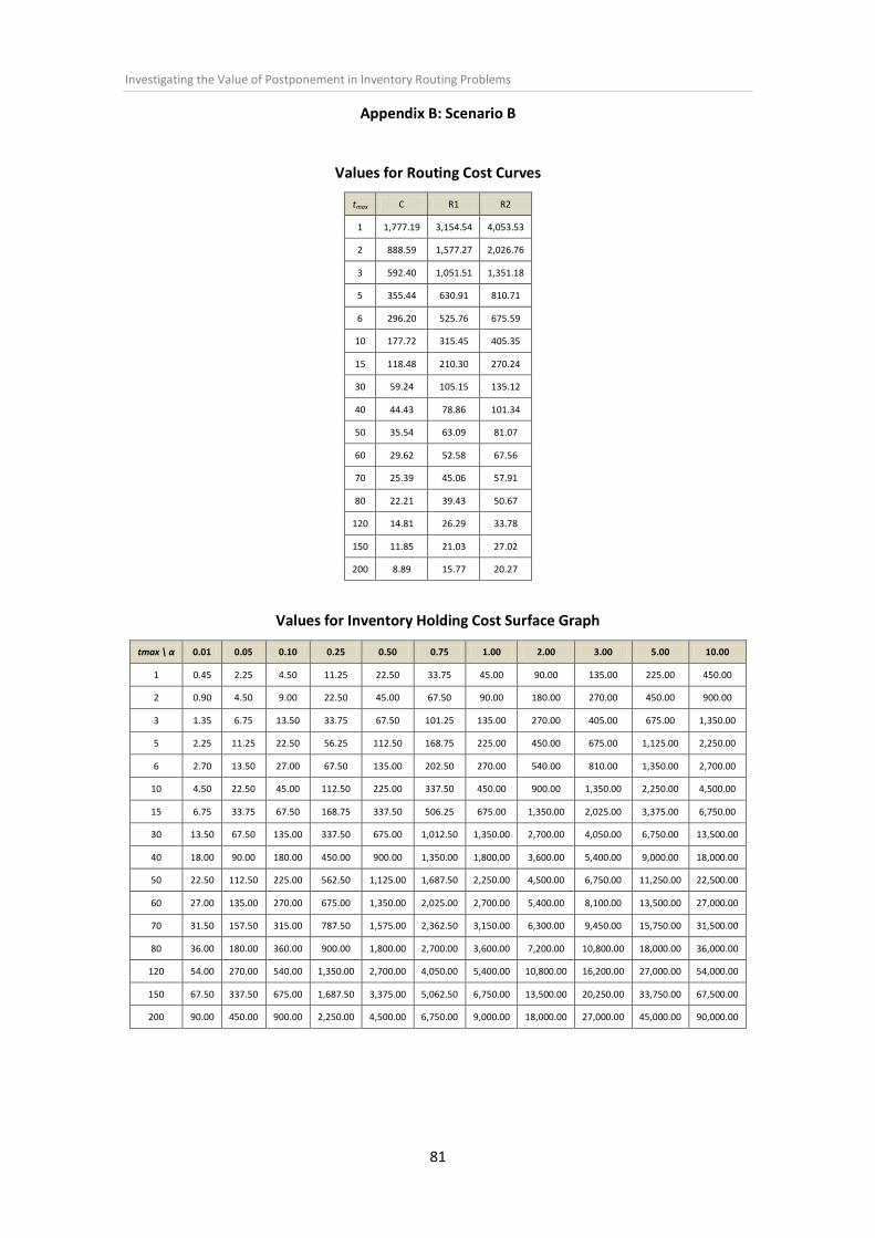
Investigating the Value of Postponement in Inventory Routing Problems
81
Appendix B: Scenario B
Values for Routing Cost Curves
tmax C R1 R2
1 1,777.19 3,154.54 4,053.53
2 888.59 1,577.27 2,026.76
3 592.40 1,051.51 1,351.18
5 355.44 630.91 810.71
6 296.20 525.76 675.59
10 177.72 315.45 405.35
15 118.48 210.30 270.24
30 59.24 105.15 135.12
40 44.43 78.86 101.34
50 35.54 63.09 81.07
60 29.62 52.58 67.56
70 25.39 45.06 57.91
80 22.21 39.43 50.67
120 14.81 26.29 33.78
150 11.85 21.03 27.02
200 8.89 15.77 20.27
Values for Inventory Holding Cost Surface Graph
tmax \ α 0.01 0.05 0.10 0.25 0.50 0.75 1.00 2.00 3.00 5.00 10.00
1 0.45 2.25 4.50 11.25 22.50 33.75 45.00 90.00 135.00 225.00 450.00
2 0.90 4.50 9.00 22.50 45.00 67.50 90.00 180.00 270.00 450.00 900.00
3 1.35 6.75 13.50 33.75 67.50 101.25 135.00 270.00 405.00 675.00 1,350.00
5 2.25 11.25 22.50 56.25 112.50 168.75 225.00 450.00 675.00 1,125.00 2,250.00
6 2.70 13.50 27.00 67.50 135.00 202.50 270.00 540.00 810.00 1,350.00 2,700.00
10 4.50 22.50 45.00 112.50 225.00 337.50 450.00 900.00 1,350.00 2,250.00 4,500.00
15 6.75 33.75 67.50 168.75 337.50 506.25 675.00 1,350.00 2,025.00 3,375.00 6,750.00
30 13.50 67.50 135.00 337.50 675.00 1,012.50 1,350.00 2,700.00 4,050.00 6,750.00 13,500.00
40 18.00 90.00 180.00 450.00 900.00 1,350.00 1,800.00 3,600.00 5,400.00 9,000.00 18,000.00
50 22.50 112.50 225.00 562.50 1,125.00 1,687.50 2,250.00 4,500.00 6,750.00 11,250.00 22,500.00
60 27.00 135.00 270.00 675.00 1,350.00 2,025.00 2,700.00 5,400.00 8,100.00 13,500.00 27,000.00
70 31.50 157.50 315.00 787.50 1,575.00 2,362.50 3,150.00 6,300.00 9,450.00 15,750.00 31,500.00
80 36.00 180.00 360.00 900.00 1,800.00 2,700.00 3,600.00 7,200.00 10,800.00 18,000.00 36,000.00
120 54.00 270.00 540.00 1,350.00 2,700.00 4,050.00 5,400.00 10,800.00 16,200.00 27,000.00 54,000.00
150 67.50 337.50 675.00 1,687.50 3,375.00 5,062.50 6,750.00 13,500.00 20,250.00 33,750.00 67,500.00
200 90.00 450.00 900.00 2,250.00 4,500.00 6,750.00 9,000.00 18,000.00 27,000.00 45,000.00 90,000.00

Investigating the Value of Postponement in Inventory Routing Problems
82
Values for Total Cost Surface Graph (C)
tmax \ α 0.01 0.05 0.10 0.25 0.50 0.75 1.00 2.00 3.00 5.00 10.00
1 1,777.64 1,779.44 1,781.69 1,788.44 1,799.69 1,810.94 1,822.19 1,867.19 1,912.19 2,002.19 2,227.19
2 889.49 893.09 897.59 911.09 933.59 956.09 978.59 1,068.59 1,158.59 1,338.59 1,788.59
3 593.75 599.15 605.90 626.15 659.90 693.65 727.40 862.40 997.40 1,267.40 1,942.40
5 357.69 366.69 377.94 411.69 467.94 524.19 580.44 805.44 1,030.44 1,480.44 2,605.44
6 298.90 309.70 323.20 363.70 431.20 498.70 566.20 836.20 1,106.20 1,646.20 2,996.20
10 182.22 200.22 222.72 290.22 402.72 515.22 627.72 1,077.72 1,527.72 2,427.72 4,677.72
15 125.23 152.23 185.98 287.23 455.98 624.73 793.48 1,468.48 2,143.48 3,493.48 6,868.48
30 72.74 126.74 194.24 396.74 734.24 1,071.74 1,409.24 2,759.24 4,109.24 6,809.24 13,559.24
40 62.43 134.43 224.43 494.43 944.43 1,394.43 1,844.43 3,644.43 5,444.43 9,044.43 18,044.43
50 58.04 148.04 260.54 598.04 1,160.54 1,723.04 2,285.54 4,535.54 6,785.54 11,285.54 22,535.54
60 56.62 164.62 299.62 704.62 1,379.62 2,054.62 2,729.62 5,429.62 8,129.62 13,529.62 27,029.62
70 56.89 182.89 340.39 812.89 1,600.39 2,387.89 3,175.39 6,325.39 9,475.39 15,775.39 31,525.39
80 58.21 202.21 382.21 922.21 1,822.21 2,722.21 3,622.21 7,222.21 10,822.21 18,022.21 36,022.21
120 68.81 284.81 554.81 1,364.81 2,714.81 4,064.81 5,414.81 10,814.81 16,214.81 27,014.81 54,014.81
150 79.35 349.35 686.85 1,699.35 3,386.85 5,074.35 6,761.85 13,511.85 20,261.85 33,761.85 67,511.85
200 98.89 458.89 908.89 2,258.89 4,508.89 6,758.89 9,008.89 18,008.89 27,008.89 45,008.89 90,008.89
Values for Total Cost Surface Graph (R1)
tmax \ α 0.01 0.05 0.10 0.25 0.50 0.75 1.00 2.00 3.00 5.00 10.00
1 3,154.99 3,156.79 3,159.04 3,165.79 3,177.04 3,188.29 3,199.54 3,244.54 3,289.54 3,379.54 3,604.54
2 1,578.17 1,581.77 1,586.27 1,599.77 1,622.27 1,644.77 1,667.27 1,757.27 1,847.27 2,027.27 2,477.27
3 1,052.86 1,058.26 1,065.01 1,085.26 1,119.01 1,152.76 1,186.51 1,321.51 1,456.51 1,726.51 2,401.51
5 633.16 642.16 653.41 687.16 743.41 799.66 855.91 1,080.91 1,305.91 1,755.91 2,880.91
6 528.46 539.26 552.76 593.26 660.76 728.26 795.76 1,065.76 1,335.76 1,875.76 3,225.76
10 319.95 337.95 360.45 427.95 540.45 652.95 765.45 1,215.45 1,665.45 2,565.45 4,815.45
15 217.05 244.05 277.80 379.05 547.80 716.55 885.30 1,560.30 2,235.30 3,585.30 6,960.30
30 118.65 172.65 240.15 442.65 780.15 1,117.65 1,455.15 2,805.15 4,155.15 6,855.15 13,605.15
40 96.86 168.86 258.86 528.86 978.86 1,428.86 1,878.86 3,678.86 5,478.86 9,078.86 18,078.86
50 85.59 175.59 288.09 625.59 1,188.09 1,750.59 2,313.09 4,563.09 6,813.09 11,313.09 22,563.09
60 79.58 187.58 322.58 727.58 1,402.58 2,077.58 2,752.58 5,452.58 8,152.58 13,552.58 27,052.58
70 76.56 202.56 360.06 832.56 1,620.06 2,407.56 3,195.06 6,345.06 9,495.06 15,795.06 31,545.06
80 75.43 219.43 399.43 939.43 1,839.43 2,739.43 3,639.43 7,239.43 10,839.43 18,039.43 36,039.43
120 80.29 296.29 566.29 1,376.29 2,726.29 4,076.29 5,426.29 10,826.29 16,226.29 27,026.29 54,026.29
150 88.53 358.53 696.03 1,708.53 3,396.03 5,083.53 6,771.03 13,521.03 20,271.03 33,771.03 67,521.03
200 105.77 465.77 915.77 2,265.77 4,515.77 6,765.77 9,015.77 18,015.77 27,015.77 45,015.77 90,015.77

Investigating the Value of Postponement in Inventory Routing Problems
83
Values for Total Cost Surface Graph (R2)
tmax \ α 0.01 0.05 0.10 0.25 0.50 0.75 1.00 2.00 3.00 5.00 10.00
1 4,053.98 4,055.78 4,058.03 4,064.78 4,076.03 4,087.28 4,098.53 4,143.53 4,188.53 4,278.53 4,503.53
2 2,027.66 2,031.26 2,035.76 2,049.26 2,071.76 2,094.26 2,116.76 2,206.76 2,296.76 2,476.76 2,926.76
3 1,352.53 1,357.93 1,364.68 1,384.93 1,418.68 1,452.43 1,486.18 1,621.18 1,756.18 2,026.18 2,701.18
5 812.96 821.96 833.21 866.96 923.21 979.46 1,035.71 1,260.71 1,485.71 1,935.71 3,060.71
6 678.29 689.09 702.59 743.09 810.59 878.09 945.59 1,215.59 1,485.59 2,025.59 3,375.59
10 409.85 427.85 450.35 517.85 630.35 742.85 855.35 1,305.35 1,755.35 2,655.35 4,905.35
15 276.99 303.99 337.74 438.99 607.74 776.49 945.24 1,620.24 2,295.24 3,645.24 7,020.24
30 148.62 202.62 270.12 472.62 810.12 1,147.62 1,485.12 2,835.12 4,185.12 6,885.12 13,635.12
40 119.34 191.34 281.34 551.34 1,001.34 1,451.34 1,901.34 3,701.34 5,501.34 9,101.34 18,101.34
50 103.57 193.57 306.07 643.57 1,206.07 1,768.57 2,331.07 4,581.07 6,831.07 11,331.07 22,581.07
60 94.56 202.56 337.56 742.56 1,417.56 2,092.56 2,767.56 5,467.56 8,167.56 13,567.56 27,067.56
70 89.41 215.41 372.91 845.41 1,632.91 2,420.41 3,207.91 6,357.91 9,507.91 15,807.91 31,557.91
80 86.67 230.67 410.67 950.67 1,850.67 2,750.67 3,650.67 7,250.67 10,850.67 18,050.67 36,050.67
120 87.78 303.78 573.78 1,383.78 2,733.78 4,083.78 5,433.78 10,833.78 16,233.78 27,033.78 54,033.78
150 94.52 364.52 702.02 1,714.52 3,402.02 5,089.52 6,777.02 13,527.02 20,277.02 33,777.02 67,527.02
200 110.27 470.27 920.27 2,270.27 4,520.27 6,770.27 9,020.27 18,020.27 27,020.27 45,020.27 90,020.27

Investigating the Value of Postponement in Inventory Routing Problems
84
Appendix C: Scenario C
Values for Routing Cost Curves
tmax C R1 R2
1 5,321.17 9,912.35 13,210.36
2 2,660.59 4,956.17 6,605.18
3 1,773.72 3,304.12 4,403.45
5 1,064.23 1,982.47 2,642.07
6 886.86 1,652.06 2,201.73
10 532.12 991.23 1,321.04
15 354.74 660.82 880.69
30 177.37 330.41 440.35
40 133.03 247.81 330.26
50 106.42 198.25 264.21
60 88.69 165.21 220.17
70 76.02 141.60 188.72
80 66.51 123.90 165.13
120 44.34 82.60 110.09
150 35.47 66.08 88.07
200 26.61 49.56 66.05
Values for Inventory Holding Cost Surface Graph
tmax \ α 0.01 0.05 0.10 0.25 0.50 0.75 1.00 2.00 3.00 5.00 10.00
1 1.50 7.50 15.00 37.50 75.00 112.50 150.00 300.00 450.00 750.00 1,500.00
2 3.00 15.00 30.00 75.00 150.00 225.00 300.00 600.00 900.00 1,500.00 3,000.00
3 4.50 22.50 45.00 112.50 225.00 337.50 450.00 900.00 1,350.00 2,250.00 4,500.00
5 7.50 37.50 75.00 187.50 375.00 562.50 750.00 1,500.00 2,250.00 3,750.00 7,500.00
6 9.00 45.00 90.00 225.00 450.00 675.00 900.00 1,800.00 2,700.00 4,500.00 9,000.00
10 15.00 75.00 150.00 375.00 750.00 1,1250 1,500.00 3,000.00 4,500.00 7,500.00 15,000.00
15 22.50 112.50 225.00 562.50 1,125.00 1,687.50 2,250.00 4,500.00 6,750.00 11,250.00 22,500.00
30 45.00 225.00 450.00 1,125.00 2,250.00 3,375.00 4,500.00 9,000.00 13,500.00 22,500.00 45,000.00
40 60.00 300.00 600.00 1,500.00 3,000.00 4,500.00 6,000.00 12,000.00 18,000.00 30,000.00 60,000.00
50 75.00 375.00 750.00 1,875.00 3,750.00 5,625.00 7,500.00 15,000.00 22,500.00 37,500.00 75,000.00
60 90.00 450.00 900.00 2,250.00 4,500.00 6,750.00 9,000.00 18,000.00 27,000.00 45,000.00 90,000.00
70 105.00 525.00 1,050.00 2,625.00 5,250.00 7,875.00 10,500.00 21,000.00 31,500.00 52,500.00 10,5000.00
80 120.00 600.00 1,200.00 3,000.00 6,000.00 9,000.00 12,000.00 24,000.00 36,000.00 60,000.00 120,000.00
120 180.00 900.00 1,800.00 4,500.00 9,000.00 13,500.00 18,000.00 36,000.00 54,000.00 90,000.00 180,000.00
150 225.00 1,125.00 2,250.00 5,625.00 11,250.00 16,875.00 22,500.00 45,000.00 67,500.00 11,2500.00 225,000.00
200 300.00 1,500.00 3,000.00 7,500.00 15,000.00 22,500.00 30,000.00 60,000.00 90,000.00 15,0000.00 300,000.00

Investigating the Value of Postponement in Inventory Routing Problems
85
Values for Total Cost Surface Graph (C)
tmax \ α 0.01 0.05 0.10 0.25 0.50 0.75 1.00 2.00 3.00 5.00 10.00
1 5,322.67 5,328.67 5,336.17 5,358.67 5,396.17 5,433.67 5,471.17 5,621.17 5,771.17 6,071.17 6,821.17
2 2,663.59 2,675.59 2,690.59 2,735.59 2,810.59 2,885.59 2,960.59 3,260.59 3,560.59 4,160.59 5,660.59
3 1,778.22 1,796.22 1,818.72 1,886.22 1,998.72 2,111.22 2,223.72 2,673.72 3,123.72 4,023.72 6,273.72
5 1,071.73 1,101.73 1,139.23 1,251.73 1,439.23 1,626.73 1,814.23 2,564.23 3,314.23 4,814.23 8,564.23
6 895.86 931.86 976.86 1,111.86 1,336.86 1,561.86 1,786.86 2,686.86 3,586.86 5,386.86 9,886.86
10 547.12 607.12 682.12 907.12 1,282.12 1,657.12 2,032.12 3,532.12 5,032.12 8,032.12 15,532.12
15 377.24 467.24 579.74 917.24 1,479.74 2,042.24 2,604.74 4,854.74 7,104.74 11,604.74 22,854.74
30 222.37 402.37 627.37 1,302.37 2,427.37 3,552.37 4,677.37 9,177.37 13,677.37 22,677.37 45,177.37
40 193.03 433.03 733.03 1,633.03 3,133.03 4,633.03 6,133.03 12,133.03 18,133.03 30,133.03 60,133.03
50 181.42 481.42 856.42 1,981.42 3,856.42 5,731.42 7,606.42 15,106.42 22,606.42 37,606.42 75,106.42
60 178.69 538.69 988.69 2,338.69 4,588.69 6,838.69 9,088.69 18,088.69 27,088.69 45,088.69 90,088.69
70 181.02 601.02 1,126.02 2,701.02 5,326.02 7,951.02 10,576.02 21,076.02 31,576.02 52,576.02 105,076.02
80 186.51 666.51 1,266.51 3,066.51 6,066.51 9,066.51 12,066.51 24,066.51 36,066.51 60,066.51 120,066.51
120 224.34 944.34 1,844.34 4,544.34 9,044.34 13,544.34 18,044.34 36,044.34 54,044.34 90,044.34 180,044.34
150 260.47 1,160.47 2,285.47 5,660.47 11,285.47 16,910.47 22,535.47 45,035.47 67,535.47 112,535.47 225,035.47
200 326.61 1,526.61 3,026.61 7,526.61 15,026.61 22,526.61 30,026.61 60,026.61 90,026.61 150,026.61 300,026.61
Values for Total Cost Surface Graph (R1)
tmax \ α 0.01 0.05 0.10 0.25 0.50 0.75 1.00 2.00 3.00 5.00 10.00
1 9.913.85 9,919.85 9,927.35 9,949.85 9,987.35 10,024.85 10,062.35 10,212.35 10,362.35 10,662.35 11,412.35
2 4.959.17 4,971.17 4,986.17 5,031.17 5,106.17 5,181.17 5,256.17 5,556.17 5,856.17 6,456.17 7,956.17
3 3.308.62 3,326.62 3,349.12 3,416.62 3,529.12 3,641.62 3,754.12 4,204.12 4,654.12 5,554.12 7,804.12
5 1.989.97 2,019.97 2,057.47 2,169.97 2,357.47 2,544.97 2,732.47 3,482.47 4,232.47 5,732.47 9,482.47
6 1.661.06 1,697.06 1,742.06 1,877.06 2,102.06 2,327.06 2,552.06 3,452.06 4,352.06 6,152.06 10,652.06
10 1.006.23 1,066.23 1,141.23 1,366.23 1,741.23 2,116.23 2,491.23 3,991.23 5,491.23 8,491.23 15,991.23
15 683.32 773.32 885.82 1,223.32 1,785.82 2,348.32 2,910.82 5,160.82 7,410.82 11,910.82 23,160.82
30 375.41 555.41 780.41 1,455.41 2,580.41 3,705.41 4,830.41 9,330.41 13,830.41 22,830.41 45,330.41
40 307.81 547.81 847.81 1,747.81 3,247.81 4,747.81 6,247.81 12,247.81 18,247.81 30,247.81 60,247.81
50 273.25 573.25 948.25 2,073.25 3,948.25 5,823.25 7,698.25 15,198.25 22,698.25 37,698.25 75,198.25
60 255.21 615.21 1,,065.21 2,415.21 4,665.21 6,915.21 9,165.21 18,165.21 27,165.21 45,165.21 90,165.21
70 246.60 666.60 1,191.60 2,766.60 5,391.60 8,016.60 10,641.60 21,141.60 31,641.60 52,641.60 105,141.60
80 243.90 723.90 1,323.90 3,123.90 6,123.90 9,123.90 12,123.90 24,123.90 36,123.90 60,123.90 120,123.90
120 262.60 9,82.60 1,882.60 4,582.60 9,082.60 13,582.60 18,082.60 36,082.60 54,082.60 90,082.60 180,082.60
150 291.08 1,191.08 2,316.08 5,691.08 11,316.08 16,941.08 22,566.08 45,066.08 67,566.08 112,566.08 225,066.08
200 349.56 1,549.56 3,049.56 7,549.56 15,049.56 22,549.56 30,049.56 60,049.56 90,049.56 150,049.56 300,049.56

Investigating the Value of Postponement in Inventory Routing Problems
86
Values for Total Cost Surface Graph (R2)
tmax \ α 0.01 0.05 0.10 0.25 0.50 0.75 1.00 2.00 3.00 5.00 10.00
1 13,211.8
6 13,217.8
6 13,225.3
6 13,247.8
6 13,285.3
6 13,322.8
6 13,360.3
6 13,510.36 13,660.36 13,960.36 14,710.36
2 6,608.18 6,620.18 6,635.18 6,680.18 6,755.18 6,830.18 6,905.18 7,205.18 7,505.18 8,105.18 9,605.18
3 4,407.95 4,425.95 4,448.45 4,515.95 4,628.45 4,740.95 4,853.45 5,303.45 5,753.45 6,653.45 8,903.45
5 2,649.57 2,679.57 2,717.07 2,829.57 3,017.07 3,204.57 3,392.07 4,142.07 4,892.07 6,392.07 10,142.07
6 2,210.73 2,246.73 2,291.73 2,426.73 2,651.73 2,876.73 3,101.73 4,001.73 4,901.73 6,701.73 11,201.73
10 1,336.04 1,396.04 1,471.04 1,696.04 2,071.04 2,446.04 2,821.04 4,321.04 5,821.04 8,821.04 16,321.04
15 903.19 993.19 1,105.69 1,443.19 2,005.69 2,568.19 3,130.69 5,380.69 7,630.69 12,130.69 23,380.69
30 485.35 665.35 890.35 1,565.35 2,690.35 3,815.35 4,940.35 9,440.35 13,940.35 22,940.35 45,440.35
40 390.26 630.26 930.26 1,830.26 3,330.26 4,830.26 6,330.26 12,330.26 18,330.26 30,330.26 60,330.26
50 339.21 639.21 1,014.21 2,139.21 4,014.21 5,889.21 7,764.21 15,264.21 22,764.21 37,764.21 75,264.21
60 310.17 670.17 1,120.17 2,470.17 4,720.17 6,970.17 9,220.17 18,220.17 27,220,.17 45,220.17 90,220.17
70 293.72 713.72 1,238.72 2,813.72 5,438.72 8,063.72 10,688.7
2 21,188.72 31,688.72 52,688.72
105,188.72
80 285.13 765.13 1,365.13 3,165.13 6,165.13 9,165.13 12,165.1
3 24,165.13 36,165.13 60,165.13
120,165.13
120 290.09 1,010.09 1,910.09 4,610.09 9,110.09 13,610.0
9 18,110.0
9 36,110.09 54,110.09 90,110.09
180,110.09
150 313.07 1,213.07 2,338.07 5,713.07 11,338.0
7 16,963.0
7 22,588.0
7 45,088.07 67,588.07
112,588.07
225,088.07
200 366.05 1,566.05 3,066.05 7,566.05 15,066.0
5 22,566.0
5 30,066.0
5 60,066.05 90,066.05
150,066.05
300,066.05

Investigating the Value of Postponement in Inventory Routing Problems
87
Appendix D: Scenario D
Values for Routing Cost Curves
Q = tmax S1 S2
1 237.29 374.86
2 59.32 93.72
3 39.55 62.48
5 11.86 18.74
6 9.89 15.62
10 5.93 9.37
15 3.95 6.25
30 1.98 3.12
40 1.48 2.34
50 1.19 1.87
60 0.99 1.56
70 0.85 1.34
80 0.74 1.17
120 0.49 0.78
150 0.39 0.62
200 0.29 0.47
Values for Inventory Holding Cost Surface Graph
Q = tmax \ α 0.01 0.05 0.10 0.25 0.50 0.75 1.00 2.00 3.00 5.00 10.00
1 0.02 0.09375 0.188 0.469 0.9375 1.4063 1.875 3.75 5.625 9.38 18.75
2 0.04 0.1875 0.375 0.938 1.875 2.8125 3.75 7.5 11.25 18.75 37.5
3 0.06 0.28125 0.563 1.406 2.8125 4.2188 5.625 11.25 16.875 28.125 56.25
5 0.09 0.46875 0.938 2.344 4.6875 7.0313 9.375 18.75 28.125 46.875 93.75
6 0.11 0.5625 1.125 2.813 5.625 8.4375 11.25 22.5 33.75 56.25 112.5
10 0.19 0.9375 1.875 4.688 9.375 14.063 18.75 37.5 56.25 93.75 187.5
15 0.28 1.40625 2.813 7.031 14.063 21.094 28.125 56.25 84.375 140.625 281.25
30 0.56 2.8125 5.625 14.06 28.125 42.188 56.25 112.5 168.75 281.25 562.5
40 0.75 3.75 7.5 18.75 37.5 56.25 75 150 225 375 750
50 0.94 4.6875 9.375 23.44 46.875 70.313 93.75 187.5 281.25 468.75 937.5
60 1.13 5.625 11.25 28.13 56.25 84.375 112.5 225 337.5 562.5 1,125
70 1.31 6.5625 13.13 32.81 65.625 98.438 131.25 262.5 393.75 656.25 1,312.5
80 1.50 7.5 15 37.5 75 112.5 150 300 450 750 1,500
120 2.25 11.25 22.5 56.25 112.5 168.75 225 450 675 1125 2,250
150 2.81 14.0625 28.13 70.31 140.63 210.94 281.25 562.5 843.75 1,406.25 2,812.5
200 3.75 18.75 37.5 93.75 187.5 281.25 375 750 1,125 1,875 3,750

Investigating the Value of Postponement in Inventory Routing Problems
88
Values for Total Cost Surface Graph (S1)
Q = tmax \ α 0.01 0.05 0.10 0.25 0.50 0.75 1.00 2.00 3.00 5.00 10.00
1 237.31 237.39 237.48 237.76 238.23 238.70 239.17 241.04 242.92 246.67 256.04
2 59.36 59.51 59.70 60.26 61.20 62.14 63.07 66.82 70.57 78.07 96.82
3 39.61 39.83 40.11 40.96 42.36 43.77 45.17 50.80 56.42 67.67 95.80
5 11.96 12.33 12.80 14.21 16.55 18.90 21.24 30.61 39.99 58.74 105.61
6 10.00 10.45 11.01 12.70 15.51 18.32 21.14 32.39 43.64 66.14 122.39
10 6.12 6.87 7.81 10.62 15.31 19.995 24.68 43.43 62.18 99.68 193.43
15 4.24 5.36 6.77 10.99 18.02 25.049 32.08 60.20 88.33 144.58 285.20
30 2.54 4.79 7.60 16.04 30.10 44.16 58.23 114.48 170.73 283.23 564.48
40 2.23 5.23 8.98 20.23 38.98 57.73 76.48 151.48 226.48 376.48 751.48
50 2.12 5.87 10.56 24.62 48.06 71.50 94.94 188.69 282.44 469.94 938.69
60 2.11 6.61 12.24 29.11 57.24 85.36 113.49 225.99 338.49 563.49 1,125.99
70 2.16 7.41 13.97 33.66 66.47 99.28 132.10 263.35 394.60 657.10 1,313.35
80 2.24 8.24 15.74 38.24 75.74 113.24 150.74 300.74 450.74 750.74 1,500.74
120 2.74 11.74 22.99 56.74 112.99 169.24 225.49 450.49 675.49 1,125.49 2,250.49
150 3.21 14.46 28.52 70.71 141.02 211.33 281.65 562.90 844.15 1,406.65 2,812.90
200 4.05 19.05 37.80 94.05 187.80 281.55 375.30 750.30 1,125.30 1,875.30 3,750.30
Values for Total Cost Surface Graph (S2)
Q = tmax \ α 0.01 0.05 0.10 0.25 0.50 0.75 1.00 2.00 3.00 5.00 10.00
1 374.88 374.96 375.05 375.33 375.80 376.27 376.74 378.61 380.49 384.24 393.61
2 93.75 93.90 94.09 94.65 95.59 96.53 97.47 101.22 104.97 112.47 131.22
3 62.53 62.76 63.04 63.88 65.29 66.70 68.10 73.73 79.35 90.60 118.73
5 18.84 19.21 19.68 21.09 23.43 25.77 28.12 37.49 46.87 65.62 112.49
6 15.73 16.18 16.74 18.43 21.24 24.06 26.87 38.12 49.37 71.87 128.12
10 9.56 10.31 11.25 14.06 18.75 23.43 28.12 46.87 65.62 103.12 196.87
15 6.53 7.65 9.06 13.28 20.31 27.34 34.37 62.50 90.62 146.87 287.50
30 3.69 5.94 8.75 17.19 31.25 45.31 59.37 115.62 171.87 284.37 565.62
40 3.09 6.09 9.84 21.09 39.84 58.59 77.34 152.34 227.34 377.34 752.34
50 2.81 6.56 11.25 25.31 48.75 72.19 95.62 189.37 283.12 470.62 939.37
60 2.69 7.19 12.81 29.69 57.81 85.94 114.06 226.56 339.06 564.06 1,126.56
70 2.65 7.90 14.46 34.15 66.96 99.78 132.59 263.84 395.09 657.59 1,313.84
80 2.67 8.67 16.17 38.67 76.17 113.67 151.17 301.17 451.17 751.17 1,501.17
120 3.03 12.03 23.28 57.03 113.28 169.53 225.78 450.78 675.78 1,125.78 2,250.78
150 3.44 14.69 28.75 70.94 141.25 211.56 281.87 563.12 844.37 1,406.87 2,813.12
200 4.22 19.22 37.97 94.22 187.97 281.72 375.47 750.47 1,125.47 1,875.47 3,750.47

Investigating the Value of Postponement in Inventory Routing Problems
89
Appendix E: Scenario E
Values for Routing Cost Curves
tmax S1 S2
1 565.84 840.98
2 282.92 420.49
3 188.61 280.33
5 113.17 168.20
6 94.31 140.16
10 56.58 84.10
15 37.72 56.07
30 18.86 28.03
40 14.15 21.02
50 11.32 16.82
60 9.43 14.02
70 8.08 12.01
80 7.07 10.51
120 4.72 7.01
150 3.77 5.61
200 2.83 4.20
Values for Inventory Holding Cost Surface Graph
tmax \ α 0.01 0.05 0.10 0.25 0.50 0.75 1.00 2.00 3.00 5.00 10.00
1 0.19 0.94 1.88 4.69 9.38 14.06 18.75 37.50 56.25 93.75 187.50
2 0.38 1.88 3.75 9.38 18.75 28.13 37.50 75.00 112.50 187.50 375.00
3 0.56 2.81 5.63 14.06 28.13 42.19 56.25 112.50 168.75 281.25 562.50
5 0.94 4.69 9.38 23.44 46.88 70.31 93.75 187.50 281.25 468.75 937.50
6 1.13 5.63 11.25 28.13 56.25 84.38 112.50 225.00 337.50 562.50 1,125.00
10 1.88 9.38 18.75 46.88 93.75 140.63 187.50 375.00 562.50 937.50 1,875.00
15 2.81 14.06 28.13 70.31 140.63 210.94 281.25 562.50 843.75 1,406.25 2,812.50
30 5.63 28.13 56.25 140.63 281.25 421.88 562.50 1,125.00 1,687.50 2,812.50 5,625.00
40 7.50 37.50 75.00 187.50 375.00 562.50 750.00 1,500.00 2,250.00 3,750.00 7,500.00
50 9.38 46.88 93.75 234.38 468.75 703.13 937.50 1,875.00 2,812.50 4,687.50 9,375.00
60 11.25 56.25 112.50 281.25 562.50 843.75 1,125.00 2,250.00 3,375.00 5,625.00 11,250.00
70 13.13 65.63 131.25 328.13 656.25 984.38 1,312.50 2,625.00 3,937.50 6,562.50 13,125.00
80 15.00 75.00 150.00 375.00 750.00 1,125.00 1,500.00 3,000.00 4,500.00 7,500.00 15,000.00
120 22.50 112.50 225.00 562.50 1,125.00 1,687.50 2,250.00 4,500.00 6,750.00 11,250.00 22,500.00
150 28.13 140.63 281.25 703.13 1,406.25 2,109.38 2,812.50 5,625.00 8,437.50 14,062.50 28,125.00
200 37.50 187.50 375.00 937.50 1,875.00 2,812.50 3,750.00 7,500.00 11,250.00 18,750.00 37,500.00

Investigating the Value of Postponement in Inventory Routing Problems
90
Values for Total Cost Surface Graph (S1)
tmax \ α 0.01 0.05 0.10 0.25 0.50 0.75 1.00 2.00 3.00 5.00 10.00
1 566.02 566.77 567.71 570.52 575.21 579.90 584.59 603.34 622.09 659.59 753.34
2 283.29 284.79 286.67 292.29 301.67 311.04 320.42 357.92 395.42 470.42 657.92
3 189.17 19.42 194.24 202.67 216.74 230.80 244.86 301.11 357.36 469.86 751.11
5 114.10 11.85 122.54 136.60 160.04 183.48 206.92 300.67 394.42 581.92 1,050.67
6 95.43 99.93 105.56 122.43 150.56 178.68 206.81 319.31 431.81 656.81 1,219.31
10 58.46 65.96 75.33 103.46 150.33 197.21 244.08 431.58 619.08 994.08 1,931.58
15 40.53 51.78 65.85 108.03 178.35 248.66 318.97 600.22 881.47 1,443.97 2,850.22
30 24.49 46.99 75.11 159.49 300.11 440.74 581.36 1,143.86 1,706.36 2,831.36 5,643.86
40 21.65 51.65 89.15 201.65 389.15 576.65 764.15 1,514.15 2,264.15 3,764.15 7,514.15
50 20.69 58.19 105.07 245.69 480.07 714.44 948.82 1,886.32 2,823.82 4,698.82 9,386.32
60 20.68 65.68 121.93 290.68 571.93 853.18 1,134.43 2,259.43 3,384.43 5,634.43 11,259.43
70 21.21 73.71 139.33 336.21 664.33 992.46 1,320.58 2,633.08 3,945.58 6,570.58 13,133.08
80 22.07 82.07 157.07 382.07 757.07 1,132.07 1,507.07 3,007.07 4,507.07 7,507.07 15,007.07
120 27.22 117.22 229.72 567.22 1,129.72 1,692.22 2,254.72 4,504.72 6,754.72 11,254.72 22,504.72
150 31.90 144.40 285.02 706.90 1,410.02 2,113.15 2,816.27 5,628.77 8,441.27 14,066.27 28,128.77
200 40.33 190.33 377.83 940.33 1,877.83 2,815.33 3,752.83 7,502.83 11,252.83 18,752.83 37,502.83
Values for Total Cost Surface Graph (S2)
tmax \ α 0.01 0.05 0.10 0.25 0.50 0.75 1.00 2.00 3.00 5.00 10.00
1 841.16 841.91 842.85 845.66 850.35 855.04 859.73 878.48 897.23 934.73 1,028.48
2 420.86 422.36 424.24 429.86 439.24 448.61 457.99 495.49 532.99 607.99 795.49
3 280.89 283.14 285.95 294.39 308.45 322.51 336.58 392.83 449.08 561.58 842.83
5 169.13 172.88 177.57 191.63 215.07 238.51 261.95 355.70 449.45 636.95 1,105.70
6 141.29 145.79 151.41 168.29 196.41 224.54 252.66 365.16 477.66 702.66 1,265.16
10 85.97 93.47 102.85 130.97 177.85 224.72 271.60 459.10 646.60 1,021.60 1,959.10
15 58.88 70.13 84.19 126.38 196.69 267.00 337.32 618.57 899.82 1,462.32 2,868.57
30 33.66 56.16 84.28 168.66 309.28 449.91 590.53 1,153.03 1,715.53 2,840.53 5,653.03
40 28.52 58.52 96.02 208.52 396.02 583.52 771.02 1,521.02 2,271.02 3,771.02 7,521.02
50 26.19 63.69 110.57 251.19 485.57 719.94 954.32 1,891.82 2,829.32 4,704.32 9,391.82
60 25.27 70.27 126.52 295.27 576.52 857.77 1,139.02 2,264.02 3,389.02 5,639.02 11,264.02
70 25.14 77.64 143.26 340.14 668.26 996.39 1,324.51 2,637.01 3,949.51 6,574.51 13,137.01
80 25.51 85.51 160.51 385.51 760.51 1,135.51 1,510.51 3,010.51 4,510.51 7,510.51 15,010.51
120 29.51 119.51 232.01 569.51 1,132.01 1,694.51 2,257.01 4,507.01 6,757.01 11,257.01 22,507.01
150 33.73 146.23 286.86 708.73 1,411.86 2,114.98 2,818.11 5,630.61 8,443.11 14,068.11 28,130.61
200 41.70 191.70 379.20 941.70 1,879.20 2,816.70 3,754.20 7,504.20 11,254.20 18,754.20 37,504.20
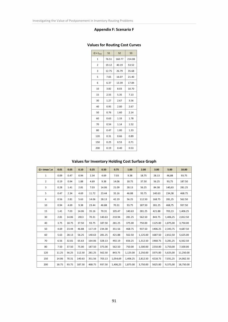
Investigating the Value of Postponement in Inventory Routing Problems
91
Appendix F: Scenario F
Values for Routing Cost Curves
Q = tmax S1 S2 S3
1 76.51 160.77 214.08
2 19.12 40.19 53.52
3 12.75 26.79 35.68
5 7.65 16.07 21.40
6 6.37 13.39 17.84
10 3.82 8.03 10.70
15 2.55 5.35 7.13
30 1.27 2.67 3.56
40 0.95 2.00 2.67
50 0.76 1.60 2.14
60 0.63 1.33 1.78
70 0.54 1.14 1.52
80 0.47 1.00 1.33
120 0.31 0.66 0.89
150 0.25 0.53 0.71
200 0.19 0.40 0.53
Values for Inventory Holding Cost Surface Graph
Q = tmax \ α 0.01 0.05 0.10 0.25 0.50 0.75 1.00 2.00 3.00 5.00 10.00
1 0.09 0.47 0.94 2.34 4.69 7.03 9.38 18.75 28.13 46,88 93.75
2 0.19 0.94 1.88 4.69 9.38 14.06 18.75 37.50 56.25 93,75 187.50
3 0.28 1.41 2.81 7.03 14.06 21.09 28.13 56.25 84.38 140,63 281.25
5 0.47 2.34 4.69 11.72 23.44 35.16 46.88 93.75 140.63 234,38 468.75
6 0.56 2.81 5.63 14.06 28.13 42.19 56.25 112.50 168.75 281,25 562.50
10 0.94 4.69 9.38 23.44 46.88 70.31 93.75 187.50 281.25 468,75 937.50
15 1.41 7.03 14.06 35.16 70.31 105.47 140.63 281.25 421.88 703,13 1,406.25
30 2.81 14.06 2813 70.31 140.63 210.94 281.25 562.50 843.75 1,406,25 2,812.50
40 3.75 18.75 37.50 93.75 187.50 281.25 375.00 750.00 1125.00 1,875,00 3,750.00
50 4.69 23.44 46.88 117.19 234.38 351.56 468.75 937.50 1406.25 2,343,75 4,687.50
60 5.63 28.13 56.25 140.63 281.25 421.88 562.50 1,125.00 1687.50 2,812,50 5,625.00
70 6.56 32.81 65.63 164.06 328.13 492.19 656.25 1,312.50 1968.75 3,281,25 6,562.50
80 7.50 37.50 75.00 187.50 375.00 562.50 750.00 1,500.00 2250.00 3,750,00 7,500.00
120 11.25 56.25 112.50 281.25 562.50 843.75 1,125.00 2,250.00 3375.00 5,625,00 11,250.00
150 14.06 70.31 140.63 351.56 703.13 1,054,69 1,406.25 2,812.50 4218.75 7,031,25 14,062.50
200 18.75 93.75 187.50 468.75 937.50 1,406,25 1,875.00 3,750.00 5625.00 9,375,00 18,750.00

Investigating the Value of Postponement in Inventory Routing Problems
92
Values for Total Cost Surface Graph (S1)
Q = tmax \ α 0.01 0.05 0.10 0.25 0.50 0.75 1.00 2.00 3.00 5.00 10.00
1 198.76 199.13 199.60 201.01 203.35 205.70 208.04 217.41 226.79 245.54 292.41
2 99.52 100.27 101.21 104.02 108.71 113.39 118.08 136.83 155.58 193.08 286.83
3 66.50 67.63 69.03 73.25 80.28 87.32 94.35 122.47 150.60 206.85 347.47
5 40.20 42.08 44.42 51.45 63.17 74.89 86.61 133.48 180.36 274.11 508.48
6 33.67 35.92 38.74 47.17 61.24 75.30 89.36 145.61 201.86 314.36 595.61
10 20.80 24.55 29.24 43.30 66.74 90.18 113.62 207.37 301.12 488.62 957.37
15 14.65 20.28 27.31 48.40 83.56 118.71 153.87 294.49 435.12 716.37 1,419.49
30 9.43 20.68 34.75 76.93 147.25 217.56 287.87 569.12 850.37 141.87 2,819.12
40 8.72 23.72 42.47 98.72 192.47 286.22 379.97 754.97 112.,97 1,879.97 3,754.97
50 8.66 27.41 50.85 121.16 238.35 355.54 472.72 941.47 1,410.22 2,347.72 4,691.47
60 8.94 31.44 59.56 143.94 284.56 425.19 565.81 1,128.31 1,690.81 2,815.81 5,628.31
70 9.40 35.65 68.46 166.90 330.96 495.03 659.09 1,315.34 1,971.59 3,284.09 6,565.34
80 9.98 39.98 77.48 189.98 377.48 564.98 752.48 1,502.48 2,252.48 3,752.48 7,502.48
120 12.91 57.91 114.16 282.91 564.16 845.41 1,126.66 2,251.66 3,376.66 5,626.66 1,125.,66
150 15.39 71.64 141.95 352.89 704.45 1,056.01 1,407.57 2,813.82 4,220.07 7,032.57 14,063.82
200 19.74 94.74 188.49 469.74 938.49 1,407.24 1,875.99 3,750.99 5,625.99 9,375.99 18,750.99
Values for Total Cost Surface Graph (S2)
Q = tmax \ α 0.01 0.05 0.10 0.25 0.50 0.75 1.00 2.00 3.00 5.00 10.00
1 367.27 367.64 368.11 369.52 371.86 374.20 376.55 385.92 395.30 414.05 460.92
2 183.77 184.52 185.46 188.27 192.96 197.65 202.34 221.09 239.84 277.34 371.09
3 122.67 123.80 125.20 129.42 136.45 143.48 150.52 178.64 206.77 263.02 403.64
5 73.90 75.78 78.12 85.15 96.87 108.59 120.31 167.18 214.06 307.81 542.18
6 61.76 64.01 66.82 75.26 89.32 103.38 117.45 173.70 229.95 342.45 623.70
10 37.65 41.40 46.09 60.15 83.59 107.03 130.47 224.22 317.97 505.47 974.22
15 25.88 31.51 38.54 59.63 94.79 129.95 165.10 305.73 446.35 727.60 1,430.73
30 15.05 26.30 40.36 82.55 152.86 223.18 293.49 574.74 855.99 1,418.49 2,824.74
40 12.93 27.93 46.68 102.93 196.68 290.43 384.18 759.18 1,134.18 1,884.18 3,759.18
50 12.03 30.78 54.22 124.53 241.72 358.91 476.09 944.84 1,413.59 2,351.09 4,694.84
60 11.74 34.24 62.37 146.74 287.37 427.99 568.62 1,131.12 1,693.62 2,818.62 5,631.12
70 11.81 38.06 70.87 169.31 333.37 497.43 661.50 1,317.75 1,974.00 3,286.50 6,567.75
80 12.09 42.09 79.59 192.09 379.59 567.09 754.59 1,504.59 2,254.59 3,754.59 7,504.59
120 14.31 59.31 115.56 284.31 565.56 846.81 1,128.06 2,253.06 3,378.06 5,628.06 11,253.06
150 16.51 72.76 143.07 354.01 705.57 1,057.14 1,408.70 2,814.95 4,221.20 7,033.70 14,064.95
200 20.59 95.59 189.34 470.59 939.34 1,408.09 1,876.84 3,751.84 5,626.84 9,376.84 18,751.84

Investigating the Value of Postponement in Inventory Routing Problems
93
Values for Total Cost Surface Graph (S3)
Q = tmax \ α 0.01 0.05 0.10 0.25 0.50 0.75 1.00 2.00 3.00 5.00 10.00
1 473.90 474.27 474.74 476.15 478.49 480.84 483.18 492.55 501.93 520.68 567.55
2 237.09 237.84 238.78 241.59 246.28 250.96 255.65 274.40 293.15 330.65 424.40
3 158.22 159.34 160.75 164.97 172.00 179.03 186.06 214.18 242.31 298.56 439.18
5 95.23 97.10 99.45 106.48 118.20 129.92 141.64 188.51 235.39 329.14 563.51
6 79.53 81.78 84.59 93.03 107.09 121.15 135.22 191.47 247.72 360.22 641.47
10 48.32 52.07 56.76 70.82 94.26 117.69 141.13 234.88 328.63 516.13 984.88
15 32.99 38.62 45.65 66.74 101.90 137.06 172.21 312.84 453.46 734.71 1,437.84
30 18.61 29.86 43.92 86.11 156.42 226.73 297.04 578.29 859.54 1,422.04 2,828.29
40 15.60 30.60 49.35 105.60 199.35 293.10 386.85 761.85 1,136.85 1,886.85 3,761.85
50 14.16 32.91 56.35 126.66 243.85 361.04 478.23 946.98 1,415.73 2,353.23 4,696.98
60 13.52 36.02 64.15 148.52 289.15 429.77 570.40 1,132.90 1,695.40 2,820.40 5,632.90
70 13.33 39.58 72.39 170.83 334.89 498.96 663.02 1,319.27 1,975.52 3,288.02 6,569.27
80 13.42 43.42 80.92 193.42 380.92 568.42 755.92 1,505.92 2,255.92 3,755.92 7,505.92
120 15.20 60.20 116.45 285.20 566.45 847.70 1,128.95 2,253.95 3,378.95 5,628.95 11,253.95
150 17.22 73.47 143.78 354.72 706.28 1,057.85 1,409.41 2,815.66 4,221.91 7,034.41 14,065.66
200 21.12 96.12 189.87 471.12 939.87 1,408.62 1,877.37 3,752.37 5,627.37 9,377.37 18,752.37
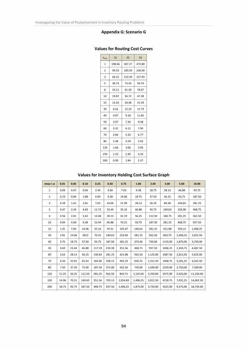
Investigating the Value of Postponement in Inventory Routing Problems
94
Appendix G: Scenario G
Values for Routing Cost Curves
tmax S1 S2 S3
1 198.66 367.17 473.80
2 99.33 183.59 236.90
3 66.22 122.39 157.93
5 39.73 73.43 94.76
6 33.11 61.20 78.97
10 19.87 36.72 47.38
15 13.24 24.48 31.59
30 6.62 12.24 15.79
40 4.97 9.18 11.85
50 3.97 7.34 9.48
60 3.31 6.12 7.90
70 2.84 5.25 6.77
80 2.48 4.59 5.92
120 1.66 3.06 3.95
150 1.32 2.45 3.16
200 0.99 1.84 2.37
Values for Inventory Holding Cost Surface Graph
tmax \ α 0.01 0.05 0.10 0.25 0.50 0.75 1.00 2.00 3.00 5.00 10.00
1 0.09 0.47 0.94 2.34 4.69 7.03 9.38 18.75 28.13 46,88 93.75
2 0.19 0.94 1.88 4.69 9.38 14.06 18.75 37.50 56.25 93,75 187.50
3 0.28 1.41 2.81 7.03 14.06 21.09 28.13 56.25 84.38 140,63 281.25
5 0.47 2.34 4.69 11.72 23.44 35.16 46.88 93.75 140.63 234,38 468.75
6 0.56 2.81 5.63 14.06 28.13 42.19 56.25 112.50 168.75 281,25 562.50
10 0.94 4.69 9.38 23.44 46.88 70.31 93.75 187.50 281.25 468,75 937.50
15 1.41 7.03 14.06 35.16 70.31 105.47 140.63 281.25 421.88 703,13 1,406.25
30 2.81 14.06 2813 70.31 140.63 210.94 281.25 562.50 843.75 1,406,25 2,812.50
40 3.75 18.75 37.50 93.75 187.50 281.25 375.00 750.00 1125.00 1,875,00 3,750.00
50 4.69 23.44 46.88 117.19 234.38 351.56 468.75 937.50 1406.25 2,343,75 4,687.50
60 5.63 28.13 56.25 140.63 281.25 421.88 562.50 1,125.00 1687.50 2,812,50 5,625.00
70 6.56 32.81 65.63 164.06 328.13 492.19 656.25 1,312.50 1968.75 3,281,25 6,562.50
80 7.50 37.50 75.00 187.50 375.00 562.50 750.00 1,500.00 2250.00 3,750,00 7,500.00
120 11.25 56.25 112.50 281.25 562.50 843.75 1,125.00 2,250.00 3375.00 5,625,00 11,250.00
150 14.06 70.31 140.63 351.56 703.13 1,054,69 1,406.25 2,812.50 4218.75 7,031,25 14,062.50
200 18.75 93.75 187.50 468.75 937.50 1,406,25 1,875.00 3,750.00 5625.00 9,375,00 18,750.00

Investigating the Value of Postponement in Inventory Routing Problems
95
Values for Total Cost Surface Graph (S1)
tmax \ α 0.01 0.05 0.10 0.25 0.50 0.75 1.00 2.00 3.00 5.00 10.00
1 198.76 199.13 199.60 201.01 203.35 205.70 208.04 217.41 226.79 245.54 292.41
2 99.52 100.27 101.21 104.02 108.71 113.39 118.08 136.83 155.58 193.08 286.83
3 66.50 67.63 69.03 73.25 80.28 87.32 94.35 122.47 150.60 206.85 347.47
5 40.20 42.08 44.42 51.45 63.17 74.89 86.61 133.48 180.36 274.11 508.48
6 33.67 35.92 38.74 47.17 61.24 75.30 89.36 145.61 201.86 314.36 595.61
10 20.80 24.55 29.24 43.30 66.74 90.18 113.62 207.37 301.12 488.62 957.37
15 14.65 20.28 27.31 48.40 83.56 118.71 153.87 294.49 435.12 716.37 1,419.49
30 9.43 20.68 34.75 76.93 147.25 217.56 287.87 569.12 850.37 141.87 2,819.12
40 8.72 23.72 42.47 98.72 192.47 286.22 379.97 754.97 112.,97 1,879.97 3,754.97
50 8.66 27.41 50.85 121.16 238.35 355.54 472.72 941.47 1,410.22 2,347.72 4,691.47
60 8.94 31.44 59.56 143.94 284.56 425.19 565.81 1,128.31 1,690.81 2,815.81 5,628.31
70 9.40 35.65 68.46 166.90 330.96 495.03 659.09 1,315.34 1,971.59 3,284.09 6,565.34
80 9.98 39.98 77.48 189.98 377.48 564.98 752.48 1,502.48 2,252.48 3,752.48 7,502.48
120 12.91 57.91 114.16 282.91 564.16 845.41 1,126.66 2,251.66 3,376.66 5,626.66 1,125.,66
150 15.39 71.64 141.95 352.89 704.45 1,056.01 1,407.57 2,813.82 4,220.07 7,032.57 14,063.82
200 19.74 94.74 188.49 469.74 938.49 1,407.24 1,875.99 3,750.99 5,625.99 9,375.99 18,750.99
Values for Total Cost Surface Graph (S2)
tmax \ α 0.01 0.05 0.10 0.25 0.50 0.75 1.00 2.00 3.00 5.00 10.00
1 367.27 367.64 368.11 369.52 371.86 374.20 376.55 385.92 395.30 414.05 460.92
2 183.77 184.52 185.46 188.27 192.96 197.65 202.34 221.09 239.84 277.34 371.09
3 122.67 123.80 125.20 129.42 136.45 143.48 150.52 178.64 206.77 263.02 403.64
5 73.90 75.78 78.12 85.15 96.87 108.59 120.31 167.18 214.06 307.81 542.18
6 61.76 64.01 66.82 75.26 89.32 103.38 117.45 173.70 229.95 342.45 623.70
10 37.65 41.40 46.09 60.15 83.59 107.03 130.47 224.22 317.97 505.47 974.22
15 25.88 31.51 38.54 59.63 94.79 129.95 165.10 305.73 446.35 727.60 1,430.73
30 15.05 26.30 40.36 82.55 152.86 223.18 293.49 574.74 855.99 1,418.49 2,824.74
40 12.93 27.93 46.68 102.93 196.68 290.43 384.18 759.18 1,134.18 1,884.18 3,759.18
50 12.03 30.78 54.22 124.53 241.72 358.91 476.09 944.84 1,413.59 2,351.09 4,694.84
60 11.74 34.24 62.37 146.74 287.37 427.99 568.62 1,131.12 1,693.62 2,818.62 5,631.12
70 11.81 38.06 70.87 169.31 333.37 497.43 661.50 1,317.75 1,974.00 3,286.50 6,567.75
80 12.09 42.09 79.59 192.09 379.59 567.09 754.59 1,504.59 2,254.59 3,754.59 7,504.59
120 14.31 59.31 115.56 284.31 565.56 846.81 1,128.06 2,253.06 3,378.06 5,628.06 11,253.06
150 16.51 72.76 143.07 354.01 705.57 1,057.14 1,408.70 2,814.95 4,221.20 7,033.70 14,064.95
200 20.59 95.59 189.34 470.59 939.34 1,408.09 1,876.84 3,751.84 5,626.84 9,376.84 18,751.84

Investigating the Value of Postponement in Inventory Routing Problems
96
Values for Total Cost Surface Graph (S3)
tmax \ α 0.01 0.05 0.10 0.25 0.50 0.75 1.00 2.00 3.00 5.00 10.00
1 473.90 474.27 474.74 476.15 478.49 480.84 483.18 492.55 501.93 520.68 567.55
2 237.09 237.84 238.78 241.59 246.28 250.96 255.65 274.40 293.15 330.65 424.40
3 158.22 159.34 160.75 164.97 172.00 179.03 186.06 214.18 242.31 298.56 439.18
5 95.23 97.10 99.45 106.48 118.20 129.92 141.64 188.51 235.39 329.14 563.51
6 79.53 81.78 84.59 93.03 107.09 121.15 135.22 191.47 247.72 360.22 641.47
10 48.32 52.07 56.76 70.82 94.26 117.69 141.13 234.88 328.63 516.13 984.88
15 32.99 38.62 45.65 66.74 101.90 137.06 172.21 312.84 453.46 734.71 1,437.84
30 18.61 29.86 43.92 86.11 156.42 226.73 297.04 578.29 859.54 1,422.04 2,828.29
40 15.60 30.60 49.35 105.60 199.35 293.10 386.85 761.85 1,136.85 1,886.85 3,761.85
50 14.16 32.91 56.35 126.66 243.85 361.04 478.23 946.98 1,415.73 2,353.23 4,696.98
60 13.52 36.02 64.15 148.52 289.15 429.77 570.40 1,132.90 1,695.40 2,820.40 5,632.90
70 13.33 39.58 72.39 170.83 334.89 498.96 663.02 1,319.27 1,975.52 3,288.02 6,569.27
80 13.42 43.42 80.92 193.42 380.92 568.42 755.92 1,505.92 2,255.92 3,755.92 7,505.92
120 15.20 60.20 116.45 285.20 566.45 847.70 1,128.95 2,253.95 3,378.95 5,628.95 11,253.95
150 17.22 73.47 143.78 354.72 706.28 1,057.85 1,409.41 2,815.66 4,221.91 7,034.41 14,065.66
200 21.12 96.12 189.87 471.12 939.87 1,408.62 1,877.37 3,752.37 5,627.37 9,377.37 18,752.37