Takustraße 7D-14195 Berlin-Dahlem

GermanyKonrad-Zuse-Zentrumfur Informationstechnik Berlin

I. VEGA1, CH. SCHUTTE1,2 AND T. CONRAD1,2

1Department of Mathematics and Computer Science, Freie Universitat Berlin, Germany

2Zuse Institute Berlin, Germany

SAIMeR: Self-adapted method for theidentification of metastable states in real-world

time series

ZIB-Report 14-16 (May 2014)

Herausgegeben vomKonrad-Zuse-Zentrum fur Informationstechnik BerlinTakustraße 7D-14195 Berlin-Dahlem

Telefon: 030-84185-0Telefax: 030-84185-125

e-mail: bibliothek@zib.deURL: http://www.zib.de

ZIB-Report (Print) ISSN 1438-0064ZIB-Report (Internet) ISSN 2192-7782

SAIMeR: Self-adapted method for the identification ofmetastable states in real-world time series

I. Vega1, Ch. Schutte1,2 and T. Conrad1,2

1Department of Mathematics and Computer Science, Freie Universitat Berlin, Germany2Zuse Institute Berlin, Germany

Abstract

In the framework of time series analysis with recurrence networks, we introduceSAIMeR, a heuristic self-adapted method that determines the elusive recurrence thresh-old and identifies metastable states in complex time series. To identify metastable statesas well as the transitions between them, we use graph theory concepts and a fuzzy par-titioning clustering algorithm. We illustrate SAIMeR by applying it to three real-worldtime series and show that it is able to identify metastable states in real-world data withnoise and missing data points. Finally, we suggest a way to choose the embedding pa-rameters used to construct the state space in which this method is performed, basedon the analysis of how the values of these parameters affect two recurrence quantitativemeasurements: recurrence rate and entropy.

Keywords. Time series analysis, application in statistical physics, recurrence quan-tification analysis, threshold, metastability, non-linear dynamics

AMS subject classifications. 37M10, 62H30, 46N55

1 Introduction

The need to understand the dynamics of complex data coming from the biological, the fi-nancial, the environmental or the medical fields, has promoted the development of manyvisualization and analysis methods.

Some of the main problems these methods face arise from the high-dimensionality, non-linearity, noise or sparsity of measurements of the real-world data they analyze. As mentionedby van der Maaten and van den Herik [1], some of the linear methods — such as PCA orClassical Multi-dimensional Scaling — and non-linear methods — such as Stochastic NeighborEmbedding or Isomaps — used for this purpose, can have some drawbacks, like not preservingboth local and global scale properties of complex data or depending on many undeterminedparameters. These problems can lead to leaving large part of the analysis open to subjectiveinterpretation.

One approach that gives information about the local, medium and global scales in high-dimensional, non-linear time series, is recurrences analysis.

The study of recurrences in measure preserving dynamical systems dates back to Poincare’sstudies at the end of the nineteenth century. Such phase space studies led to the develop-ment of the concept of recurrence plot by Eckmann et al. in 1987 [2], which focused onhigh-dimensional phase space trajectories. Over the years, the study of recurrences movedfrom the qualitative to the quantitative analysis, which in turn led to the introduction ofrecurrence quantitative analysis by Zbilut and Webber in 1992 [3]. This allowed the analysisof non-linear, non-stationary time series data and broadened the concept of recurrence.

1

One of the problems of recurrence plots analysis is the selection of the parameter necessaryto compute them: the recurrence threshold. The recurrence threshold controls how close twophase space trajectories, or state space vectors, should be in order to consider them asneighbors. Therefore, it determines the size of neighborhoods in phase space that can beassociated with the existence of stable dynamical states.

More recently, Krishnan et al. in 2008 [4, 5] made the analogy of recurrence plots withgraph theory and introduced the concept of recurrence network. In 2012, Donges et al. [6]introduced some graph theory concepts to the study of recurrence networks in order toaddress the problem of selecting a recurrence threshold appropriate to analyze time serieswith uniform probability density distributions. For these cases, they set bounds in terms ofthe critical edge density of a recurrence network.

However, selecting an appropriate recurrence threshold for real-world time series is still anopen problem [7,8], due to some properties of these time series, like: a non-necessarily uniformprobability distribution, frequently having noise or missing some measurement points, andshowing metastability — a property of physical phenomena with multiple time scales in whichsome time scales are in equilibrium and produce the so called metastable states, while othersare not.

In this paper we introduce a heuristic method, based on recurrence network analysis,which identifies different metastable states in real-world time series data. This method iscalled the Self-adapted method for the identification of metastable states in real-world timeseries (SAIMeR).

The main components of SAIMeR are: computing an appropriate recurrence threshold forthe analysis of real-world time series with recurrence networks theory, identifying metastablestates in real-world time series, and providing the possibility of identifying the transitionsbetween these states due to the use of the MSM clustering algorithm [9–12].

This paper contains the detailed explanation of the construction of this method andillustrates its performance in the following way:

Section 2 presents the theoretical foundations of recurrence plots and recurrence networks:it explains the construction of the state space and the problem of selecting a recurrencethreshold. Furthermore, it contains a brief review of network clustering theory.

Section 3 explains the two parts in which SAIMeR is divided (summarized in Algorithms1, 2 and 3).

Sections 4 and 5 validate the ability of this method to identify metastable states in real-world time series in a robust way.

Section 4 illustrates the performance of SAIMeR in application to three time series show-ing metastability. The time series analyzed are: (1) the one-dimensional movement of aparticle under the gradient of a double well potential and a random force, (2) the two-dimensional molecular dynamics of Trialanine, and (3) the one-dimensional real-world timeseries containing the average daily temperatures in Berlin from 1937 to 2010.

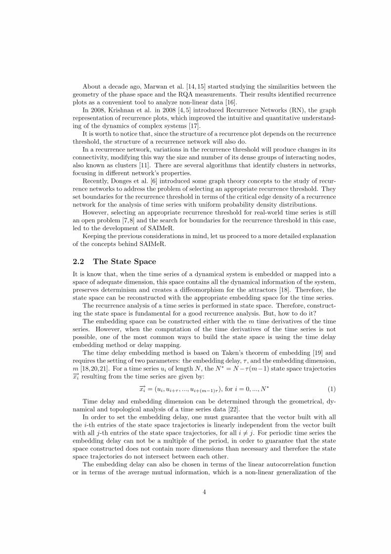
Fig. 1 contains the results of applying SAIMeR to the time series containing the averagedaily temperatures of Berlin, in the period from January 1st, 1942 to December 31st, 1943.Temperature time series are likely to have trends, possibly associated to climate change,and several missing measurement points during some periods of time (non-equally spacedmeasurements), possibly related to historical events. In Fig. 1, the gray-scale color codeindicates three different groups of time points. Two of them, the metastable states, indicatingbroadly a warm and a cold season. The third group indicates the transition regime betweenwarm and cold seasons.

The validation of the robustness of SAIMeR is contained in Section 5. For this purpose,we measure the similarity between the results obtained from two different time series: acontrol time series and a time series produced (a) by adding a percentage of noise or (b)

2

Figure 1: This figure shows the time series containing the daily average temperatures in Berlin (Tempelhof)from January 1, 1942 to December 31, 1943. The grayscale color code represents the different metastablestates identified using ε∗ ' 0.2933, τ = 2 and m = 2. For more details see Sections 4.3 and 2.

by removing a percentage of data measurements from the control time series. These twofeatures (noise and missing data points) are called artifacts.

Finally, in appendix A we suggest a way to determine the better suited embedding pa-rameters for the construction of state space based on two RQA measurements: recurrencerate and entropy.

2 Background

The method introduced in this paper, SAIMeR, is based on recurrence analysis and networkclustering analysis. Therefore, we will briefly introduce the main concepts of both theories.

2.1 Overview

Recurrence Plots were introduced by Eckmann et al. in 1987 [2] with the aim of understandingthe dynamics of complex data sets. These are inspired by Poincare’s phase space studies [13].A phase space, or state space, contains all the dynamical states of a system. Therefore,recurrence plots are computed in state space.

A recurrence plot is a tool to obtain meaningful empirical information from high-dimen-sional data sets which depends on few parameters. It is given by a square binary matrix,Rij(ε), which contains information about the recurrences of phase space trajectories, or statespace vectors, to neighborhoods that can be associated with the existence of stable dynamicalstates. The size of these neighborhoods is given by the Recurrence Threshold, ε. This way,variations in the recurrence threshold will reveal different scales of structure in the statespace.

In order to obtain not only empirical but quantitative information from a recurrence plot,Zbilut and Webber [3] introduced in the mid-nineties the so called Recurrence QuantitativeAnalysis (RQA) measurements. These measurements are computed from the recurrence plotof a given system and give information about its local, medium and global scales.

3

About a decade ago, Marwan et al. [14, 15] started studying the similarities between thegeometry of the phase space and the RQA measurements. Their results identified recurrenceplots as a convenient tool to analyze non-linear data [16].

In 2008, Krishnan et al. in 2008 [4, 5] introduced Recurrence Networks (RN), the graphrepresentation of recurrence plots, which improved the intuitive and quantitative understand-ing of the dynamics of complex systems [17].

It is worth to notice that, since the structure of a recurrence plot depends on the recurrencethreshold, the structure of a recurrence network will also do.

In a recurrence network, variations in the recurrence threshold will produce changes in itsconnectivity, modifying this way the size and number of its dense groups of interacting nodes,also known as clusters [11]. There are several algorithms that identify clusters in networks,focusing in different network’s properties.

Recently, Donges et al. [6] introduced some graph theory concepts to the study of recur-rence networks to address the problem of selecting an appropriate recurrence threshold. Theyset boundaries for the recurrence threshold in terms of the critical edge density of a recurrencenetwork for the analysis of time series with uniform probability density distributions.

However, selecting an appropriate recurrence threshold for real-world time series is stillan open problem [7,8] and the search for boundaries for the recurrence threshold in this case,led to the development of SAIMeR.

Keeping the previous considerations in mind, let us proceed to a more detailed explanationof the concepts behind SAIMeR.

2.2 The State Space

It is know that, when the time series of a dynamical system is embedded or mapped into aspace of adequate dimension, this space contains all the dynamical information of the system,preserves determinism and creates a diffeomorphism for the attractors [18]. Therefore, thestate space can be reconstructed with the appropriate embedding space for the time series.

The recurrence analysis of a time series is performed in state space. Therefore, construct-ing the state space is fundamental for a good recurrence analysis. But, how to do it?

The embedding space can be constructed either with the m time derivatives of the timeseries. However, when the computation of the time derivatives of the time series is notpossible, one of the most common ways to build the state space is using the time delayembedding method or delay mapping.

The time delay embedding method is based on Taken’s theorem of embedding [19] andrequires the setting of two parameters: the embedding delay, τ , and the embedding dimension,m [18,20,21]. For a time series ui of length N , the N∗ = N−τ(m−1) state space trajectories−→xi resulting from the time series are given by:

−→xi = (ui, ui+τ , ..., ui+(m−1)τ ), for i = 0, ..., N∗ (1)

Time delay and embedding dimension can be determined through the geometrical, dy-namical and topological analysis of a time series data [22].

In order to set the embedding delay, one must guarantee that the vector built with allthe i-th entries of the state space trajectories is linearly independent from the vector builtwith all j-th entries of the state space trajectories, for all i 6= j. For periodic time series theembedding delay can not be a multiple of the period, in order to guarantee that the statespace constructed does not contain more dimensions than necessary and therefore the statespace trajectories do not intersect between each other.

The embedding delay can also be chosen in terms of the linear autocorrelation functionor in terms of the average mutual information, which is a non-linear generalization of the

4

first and tells us how much information about ui+τ we get when we observe ui. Since twomeasurements are completely independent when the mutual information is zero, the timedelay τ can be chosen as the one for which we obtain the first minimum in average mutualinformation. However, for some systems, the mutual information might not have a minimum.In these cases, a deeper analysis is required. For an extended discussion on how to determinethe embedding time delay, see the article of Abarbanel in 1996 [21].

To set the embedding dimension, different geometrical, dynamical and topological testscan be used. The geometrical tests indicate the variations in distance between two closepoints when the embedding dimension increases, e.g. the computation of fractal dimensionsor false nearest neighbors. The dynamical tests are used to select the embedding that providesa unique future for every data point, e.g. the implementation of predictability tests or theestimation of Lyapunov exponents. The topological tests look for the embedding dimensionm that avoids intersections of stable periodic orbits. One-dimensional chaotic data, forexample, have embedding dimension m ≥ 3. Generally, for n-dimensional dynamical systemswith fractal dimension dA, the embedding dimension is m > 2dA. Another general estimationgiven by Whitney et al. [20] states that m < 2n.

Different selections of embedding parameters will reconstruct state spaces with differ-ent dynamical information quality. The recurrences in these spaces will also vary and thestructure of recurrence plots and networks will differ as well.

2.3 Recurrence Plots

The recurrence states of the state space reconstructed from complex, high-dimensional datasets can be identified with recurrence plots. A recurrence plot is defined in terms of a squarebinary matrix Rij(ε) containing information about the recurrences of state space trajectories−→xi to a set of states:

Rij(ε) = Θ (ε− d(−→xi ,−→xj))− δij (2)

In this expression, Θ(·) is a Heaviside function, d(−→xi ,−→xj) = dij is a metric and ε is the re-currence threshold – a cutoff distance that determines the size of a recurrence neighborhood – .Throughout this article, we will use the adequately scaled Euclidean metric, so that everyvariable of a time series is min-max normalized. The selection of norm implies that recur-rence neighborhoods are hyperspherical. For a detailed explanation of the effects of choosinga different metric, see article of Donner et. al from 2010 [23].

In a recurrence plot, rows represent each of the state space vectors associated to the timeseries. This way, every entry (column) j of row i represents the closeness between state spacevectors i and j.

2.4 Recurrence Networks

Every recurrence plot, Rij(ε), has an associated recurrence network, Gij(ε). In a recurrencenetwork, every node represents one of the state space vectors associated to the time seriesand every edge represents the belonging of a pair of state space vectors to a same recurrenceneighborhood. Due to the symmetry of recurrence plots, recurrence networks are unweighted,undirected and have the same number of nodes as the number of state space vectors builtfrom the data set.

The information about the local, medium and global geometric properties of a system, canbe recovered from the recurrence network through measurements based on neighborhoods oron paths. Donner et al. [24] have provided a summary of the definition and meaning of path-and neighborhood-based measurements for recurrence networks.

5

(a) Recurrence Plot (b) Recurrence Network

Figure 2: The left figure shows a recurrence plot, Rij(ε), in which every column corresponds to a differentstate space vector. If the distance between state space vectors i and j is less than the recurrence thresholdε, then Rij(ε) = 1. Otherwise, Rij(ε) = 0. Half of the plot is shown because Rij(ε) = Rji(ε). The rightfigure shows a recurrence network, Gij(ε), in which every node represents a state space vector and an edgebetween nodes i and j indicates that Rij(ε) = 1.

Since the structure of a recurrence network depends on the closeness between state spacevectors, we suggest that the regions that phase space trajectories visit the most, or recurrenceregions, should originate clusters in a recurrence network.

2.5 The Problem of Selecting an Appropriate Recurrence Threshold

The recurrence threshold, ε, determines whether two state space vectors are close or not and,therefore, it also determines the structure – its size and number of clusters – of the recurrencenetwork associated to a time series. This way, an adequate recurrence threshold could revealstructures in different scales within the state space, provide good estimations of the network’sproperties and assure a better understanding of a complex system.

The problem of selecting an appropriate recurrence threshold has been largely studied.A summary of the problems associated to the selection of the recurrence threshold is givenin an article of Donner et al. from 2010 [7].

Initially, the recurrence threshold was set “using rules of thumb” [23,24] over some dynam-ical measurements such as the correlation integrals [25], correlation dimensions [26], secondorder Renyi entropy [27,28] or attractor dimensions [7].

Generally, the recurrence threshold was kept as small as possible. Recurrence networkswith low edge densities were preferred because higher edge density values tend to hide im-portant dynamical structures. Additionally, it was desired that a small variation in therecurrence threshold did not produce noticeable differences in the dynamical analysis results.

Recently, Donges et al. [6] introduced an analytical framework, based on random geomet-ric graphs (RGGs) theory, to analyze recurrence networks. For an extended discussion onrandom graphs, see the article of Dall and Christensen form 2002 [29].

Considering RGG theory, the recurrence threshold for one-dimensional, non-noisy timeseries with uniform probability density distribution, is determined in terms of the percolationthreshold εc, which points out the limit in which the network’s giant component breaks downand makes impossible to recover information about mesoscopic and path-based measures [30].

For too large ε, the recurrence network becomes too dense, and for too small ε, therecurrence network’s giant component breaks down into smaller disconnected components.

6

In both cases the fine geometry of the time series is not well represented by the neighborhood-and path-measurements. This way, Donges et al. focused on the study of the average pathlength, which relates to the network’s giant component, to set a range of values for therecurrence threshold.

Some approaches to the analysis of recurrence networks constructed from time series withnon-uniform distributions are the study of changes in connectivity by Hsing and Rootze [31],and more recently by Cooper and Frieze [32]. On the other hand, Kong and Yeh [33] haveinvestigated the problem of characterizing the critical density and critical mean degree ofrandom geometric graphs with non-uniform probability distributions and, based on prob-abilistic methods and clustering analysis, they have provided lower bounds for the criticaldensity of a Poisson RGG in an m-dimensional Euclidean space.

2.6 Clustering Analysis

As we mention before, we are interested in identifying different metastable states in real-world time series. Thus, we combine the idea that there is a recurrence threshold for whicha recurrence network’s giant component breaks down into smaller disconnected components,with the idea that recurrence network’s clusters correspond to metastable states.

This way, we suggest to look at the results of performing clustering analysis on a recurrencenetwork in order to determine the recurrence threshold that allows the identification of allrelevant metastable states in a system.

As mentioned before, the problem of finding clusters, or modules, in complex networks hasbeen approached in several ways and many clustering algorithms exist for this purpose [11].However, we use the Markov State Model (MSM) clustering algorithm introduced by Sarich,Djurdjevac and collaborators [9, 12].

The MSM clustering algorithm is based on spectral analysis of random walks on modularnetworks and identifies modules as the metastable states in the random walker and a transi-tion region, composed with the nodes that do not belong to metastable states of the randomwalker or outliers.

In computational terms, this algorithm scales linearly with the size of the network, makingit also useful for analyzing large networks.

Since the MSM clustering algorithm gives more refined information about a network, wesuggest that using it to analyze a recurrence network will allow us to perform a more refinedquantitative analysis of recurrences in state space. And this, in turn, will help us to setboundaries for a recurrence threshold.

3 SAIMeR: Self-adapted method for the identificationof metastable states in real-world time series

Summarizing, SAIMeR is a method for the identification of metastable states in complex realwold time series. It is based on the theories of recurrence analysis and network clusteringand is therefore divided in two parts, each one focused on one of these theories. This methodis described in Algorithms 1, 2 and 3, given below.

The recurrence analysis part of SAIMeR is divided in two steps: (a) the reconstructionof state space from a time series and (b) the definition of a set of recurrence thresholds andthe construction of its associated recurrence networks.

The clustering part of SAIMeR is divided in three steps: (a) the clustering of the set ofrecurrence networks previously obtained, (b) the selection of a subset of recurrence networkswith “similar characteristics” and the recurrence thresholds producing them, and (c) the

7

Table 1: Recurrence Analysis Algorithm

• Construct the state spaceConstruct N∗ = N − (m− 1)τ state space vectors with specific embedding parameters τ andm as in Eq. 1 from min-max normalized time series containing N data points.

• Define set of recurrence thresholds and its associated networksCompute initial recurrence threshold ε0 as in Eq. 4.for ν = 0 to ν = νf do

. Compute recurrence threshold εν as in Eq. 5.

. Compute its associated recurrence plot Rν .

. Compute its associated recurrence network Gν .end forreturn Sets of recurrence thresholds εν and recurrence networks Gij(εν)

computation of a final recurrence threshold from the subset of recurrence thresholds producingsuch subset of networks and the identification of metastable states (and transition region) ina time series.

3.1 Part I: recurrence analysis

As mentioned above, the first part of SAIMeR is divided in two steps. These are explainedin Algorithm 1.

The first step consists on the construction of state space from a time series. The secondstep consists on the definition of a set of recurrence thresholds – based on basic statisticalanalysis of the data set – and the construction of its associated recurrence networks. Let uslook at these steps more carefully.

3.1.1 Constructing the state space

The first step in the recurrence analysis part of SAIMeR is the construction of the statespace from a given time series normalized to the maximum in an interval going from zero toone. We reconstruct the state space using the time delay embedding method, mentioned inSection 2.2.

The time delay embedding method requires setting two parameters: the embedding de-lay and the embedding dimension. Different selections of embedding parameters lead statespaces containing different dynamical information. Thus, the recurrence regions identified instate spaces constructed with different embedding parameters will vary. Consequently, itsrecurrence quantitative information will vary as well.

This way, we suggest that the analysis of RQA measurements can be used to determine theembedding parameters that better describe the dynamics of a time series. In Appendix A weanalyze the changes in entropy and recurrence rate of the recurrence plots associated to thesame time series but in state spaces constructed with different embedding parameters. There,we suggest a way to choose the embedding parameters. This suggestion is used throughoutthis paper to determine the embedding parameters in each of the examples used to illustrateSIMeR.

8

3.1.2 Defining a set of recurrence thresholds

The second step in the recurrence analysis part of SAIMeR is the definition of a set ofrecurrence thresholds. For this purpose, we require some knowledge about the time seriesanalyzed.

One of the distinctive features of real-world time series is the presence of artifacts such asnoise, missing or wrong measurement points, or non-uniform probability distributions. Dueto these artifacts, the results of the recurrence analysis of real-world time series can be verydifferent from the results obtained when analyzing time series without artifacts.

We suggest to compute the recurrence threshold, ε, in terms of the second moment of thetime series distribution. However, we do not use the standard deviation of the time series, σ,but assume that our data is a sample of a larger distribution and therefore use the standarderror of the mean SEx = σ√

N. The standard error of the mean measures the probability

of a sample’s mean to be close to the data set’s mean. Even for non-uniform probabilitydistributions, the standard error of the mean defines boundaries for the uncertainty in thevalue of a random variable with finite variance.

We determine the recurrence threshold to be equal to a fraction α of the smallest standarderror of the mean SEx of the data sample. This way, an initial guess for a recurrence thresholdε0, considering the previous restrictions, is given by:

ε0 = ασ√N

(3)

Varying the fraction α implies varying the size of the minimum number of recurrences.This can also be understood as varying the number of nodes required for a neighborhood tobe recurrent. We set α = 0.05N since this corresponds to the 5% error usually accepted aserror in accurate statistical analyses. This way the initial guess for the recurrence thresholdis:

ε0 = 0.05√Nσ (4)

For multi-dimensional data we compute the standard error of the mean for every variable,or dimension, and take the largest value to compute the initial recurrence threshold, usingthe same expression as for one-dimensional data. Selecting the largest standard error ofthe mean from all variables, we lose smaller scale information. This could be overcome bypreviously normalizing all variables to the value of the smallest standard deviation.

Another possible treatment could involve computing a different recurrence threshold forevery variable of the time series. This way we would compute a matrix of standard errors ofthe mean. However, we decide to focus in the dynamics of the variable that varies the most.

Once we have computed the initial recurrence threshold, we compute a set of thresholdsεν. Every element of εν is given by:

εν = (1.5− 0.1ν) ε0, for ν = [0, νf ] (5)

The size of set εν is determined by νf . We set νf = 14 in order to vary the recurrencethreshold from 0.005N to 0.075N times the standard error of the mean. We suggest that,this way, small variations in fraction α in Eq. 3 will not affect dramatically our results.

Finally, with every recurrence threshold εµ ∈ εν we will compute a recurrence plot,Rµ = Rij(εµ), and an associated recurrence network, Gµ = Gij(εµ), as described in Sections2.3 and 2.4. This way, we obtain the set of recurrence networks, Gν, computed with eachof the recurrence thresholds in set εν.

9

Table 2: Clustering analysis algorithm (Part 1)

• Cluster set of recurrence networksfor ν = 0 to ν = νf do

. Perform clustering analysis of the associated recurrence network Gij(εν).

. Compute number of clusters C(εν) and number of nodes in each cluster |Ck(εν)| ofGν .

end for

• Select subset of similar networksSelect subset of thresholds εν− such that conditions in Eq. 6 hold.for χj = [χ0, χj∗ ] and χj as in Eq. 8 do

for all ελ ∈ εν− doif |Ck(ελ+1)| − |Ck(ελ)| < χj , as in Eq. 8 then

Add recurrence threshold ελ to subset ενχj

end ifend forif ενχj 6= ∅ then

if j 6= j∗ thenContinue

elsereturn εν∗ = ενχj

end ifelse

χj! = χ(j−1)

return εν∗ = ενχj!

end ifend for

3.2 Part II: clustering analysis

The second part of SAIMeR has three steps. These are explained in Algorithms 2 and 3.The first step is the clustering analysis (number and size of clusters) of the recurrence

networks, obtained in the previous part.The second step consists on the selection of the subset of networks with similar number

and size of clusters. The set of recurrence thresholds producing such set is denoted by εν∗.Finally, the third step consists on computing the final recurrence threshold ε∗, as the

average value of recurrence thresholds in εν∗.The clustering analysis of the recurrence network produced with the final recurrence

threshold, G∗ = Gij(ε∗), leads to the identification of metastable states (and transitionregion) in the time series.

3.2.1 Clustering analysis of the set of associated recurrence networks

Every recurrence network in the set Gν of all recurrence networks associated to recurrencethresholds in set εν, will have a different structure.

The clustering analysis of a recurrence network Gµ ∈ Gν will indicate the number ofclusters in the network and the number of nodes in each cluster.

10

Table 3: Clustering analysis algorithm (Part 2)

• Identify Metastable States. Compute ‘final recurrence threshold’, ε∗, as the average value from subset εν∗.. Perform clustering analysis of the associated recurrence network G∗ = Gij(ε∗).. Classify time points into different dynamical states as in Section 3.2.3, according to

their belonging to a particular cluster in the recurrence network G∗.

Every cluster identified in a recurrence network will represent a different metastable statein the time series producing such network. When we also want to know the number ofnodes identified as part of the transition region (using the MSM clustering algorithm), weassign them to an extra cluster. What we obtain with this extra cluster is that the sumof all nodes in a cluster for every recurrence network Gµ ∈ Gν is the same and equal toN∗ = N − τ(m− 1).

A comparison of the clustering results for every recurrence network in Gν can be rep-resented with Sankey diagrams. A Sankey diagram is a flow diagram showing the change inclustering results between networks. For an example of a Sankey diagram, see Fig. 17 inAppendix C.

In a Sankey diagram, every network is represented as a column and every column isdivided into blocks. The number of blocks in a column represents the number of clustersidentified in a network. The size of a block in a column is determined by the number of nodessuch cluster contains. This way, if a group of nodes in network A are assigned to a differentcluster in network B, the Sankey diagram of these networks will show, as an arrow, the flowof such nodes from one block in column A to a different block in column B. The thickness ofsuch arrow will be determined by the amount of nodes flowing.

3.2.2 Tuning the Final Recurrence Threshold

Analyzing the different clustering results of recurrence networks in Gν, we will obtain afinal recurrence threshold, ε∗. The way to compute this final recurrence threshold constitutesthe self-adaptive part of SAIMeR.

The first step to obtain the final recurrence threshold is to identify in Gν a subset ofrecurrence networks with the same number of clusters, Gν−. From such set of recurrencenetworks one can define the subset of recurrence thresholds εν−.

Given two recurrence networks Gµ and Gµ+1 ∈ Gν, the number of clusters in them isthe same if the following conditions hold:

C(εµ+1)− C(εµ) = 0C(εµ)− C(εµ−1) = 0

C(εµ) > 1 (6)

Where C(εµ) is the number of clusters in recurrence network Gµ ∈ GνThe next step consists of selecting from Gν− a subset of recurrence networks with

clusters of similar sizes, Gνχj . Here, χj is a value, or tolerance, measuring the similaritybetween the size of clusters. The set of recurrence thresholds producing the networks withclusters of similar sizes, is denoted by ενχj .

For Ck(ελ) denoting the k-th cluster of recurrence network Gλ ∈ Gν−, and |Ck(ελ)|denoting the number of nodes in such cluster. Then, the size of every cluster in a pair of

11

consecutive recurrence networks Gλ, Gλ+1 ∈ Gν− varies less than a specified tolerance χ0,if:

|Ck(ελ+1)| − |Ck(ελ)| < χ0, for ελ ∈ εν− (7)

In Eq. 7, the tolerance depends on the number of nodes in a recurrence network, N∗, sothat χ0 = χ0(N∗). Initially, two k-th clusters in Gλ, Gλ+1 ∈ Gν− will have similar size ifthe number of nodes they contain is different in no more than ten percent the total numberof nodes in the recurrence network, or χ0(N∗) = 0.1N∗.

Initial tolerance χ0 is later decreased in order to restrict the condition of similarity betweenclusters. The extreme of similarity will be reached with tolerance χj∗ , when the number ofnodes in the k-th clusters of Gλ, Gλ+1 ∈ Gν− is different in no more than one percent thetotal number of nodes in the recurrence network, or χj∗(N∗) = 0.1N∗.

The reduction of tolerance we propose consists of only ten steps, which implies thatj∗ = 9. This way, every reduced tolerance χj ∈ [χ0, χj∗ ], is given by:

χj = χ0(1− j), for j = [0, j∗] (8)

If the subset of recurrence thresholds sufficing the maximum decrease of tolerance χj∗ isnot empty, then εν∗ = ενχj∗ .

However, this will not always occur, since not all the sets of recurrence networks associatedto εν− will suffice the maximum tolerance decrease. If the subset of recurrence thresholdssufficing the decrease of tolerance is empty for a j > j!, then εν∗ will be the last subset ofrecurrence thresholds that suffices Eq. 7, it means the average of ενχj! .

The final recurrence threshold, ε∗, will be the average of thresholds in εν∗.

3.2.3 Identification of Metastable States in the Time Series

Once that the final recurrence threshold ε∗ has been computed, we generate the recurrencenetwork associated to it, G∗ = Gij(ε∗). We identify the different metastable states in thetime series by clustering this recurrence network.

As we mentioned in Section 2.4, each node in a recurrence network represents a statespace vector in the state space reconstructed from the time series. Since we use the delaymapping to obtain the state space from the time series, each component of a state spacevector corresponds to a data point in a time series. Therefore, each node in a recurrencenetwork represents a collection of time point measurements, and the size of this collectiondepends on the embedding dimension.

In this paper, for simplicity, if node i of G∗ has been assigned to a specific cluster Ck,the data point ui in the first component of state space vector −→x i is assigned to the k-thmetastable state.

This metastable state assignment approach is naıve since, for an embedding dimensionm, every data point ui appears in up to m+ 1 state space vectors. The total number M(ui)of state space vectors in which a data point appears ui, is variable.

Therefore, the metastable state to which data point ui is assigned, should be determinedfrom the cluster assignment of M(ui) nodes in the final recurrence network. This means thatthe metastable state of data point ui is given in terms of an average cluster number Ci anda threshold θ∗ by:

Ci =1

M(ui)

∑−→x j

Cj

c(ui) = δ(Ci − θ) (9)

12

Given that the state space vectors are computed using time delay embedding, M(ui) fordata points ui such that βτ ≤ i ≤ (β + 1)τ , for β ∈ N, 0 ≤ β < m, is equal to β + 1. Fordata points ui with N − (m− α)τ ≤ i ≤ N − (m− α− 1)τ , for α ∈ N, 0 ≤ α < m− 1, thenM(ui) = m− α+ 1. Any other data point has M(ui) = m+ 1.

4 Examples

To illustrate the ability of SAIMeR to identify metastable states in complex time series, wepresent and analyze three cases. We identify the different metastable states in each of thesetime series.

The first example corresponds to the one-dimensional time series describing the motionof a particle under the gradient of a double well potential and a random force. This is oneof the simplest systems showing metastability.

The second example corresponds to a two-dimensional time series describing the moleculardynamics of trialanine, i.e. the variation of two of the three torsion angles describing itsconformation (see Fig. 6), in order to identify its main molecular conformations.

In the third example we analyze a one-dimensional real-world time series containing theaverage daily temperatures of Berlin from June 12th, 1936 to January 9th, 2008. This timeseries is likely to have trends, possibly associated to climate change, and several missing mea-surement points during some periods of time (non-equally spaced measurements), possiblyrelated to historical events.

As the results of these three examples suggest, having more accurate data improve theidentification of metastable states in the time series with SAIMeR.

4.1 Double Well Potential

The double well potential is a simple one-dimensional system showing metastability. For thisreason, this is the initial example to illustrate SAIMeR.

The time series analyzed in this section corresponds to the simulated motion of a particle,in a heat bath with temperature T , under the gradient of a double well potential and a randomforce. Such motion can be modeled with the following equation:

dXt = −∇V (x)dt+√

2εdBt (10)

In this equation, Bt is a Brownian motion, ε = νT , ν > 0 is a friction parameter and Tis the temperature of the heat bath. V (x) = (x2 − a2)2, is a double well potential with twolocal minima at x1 = a and x2 = −a. In this case we set a = 1.

The double well potential model in Eq. 10 is one of the first models for metastability. Itwas proposed by Kramer in 1949 [34], during his studies on chemical reactions. Fig. 3 showsa representation of the double well potential V (x) = (x2− 1)2. In this figure, ∆V is the trapdepth difference between the potential wells which controls how metastable the system is.

The double well potential time series is shown in Fig. 4 and results from integrating thedouble well potential’s Langevin dynamical equations. For this, we use the Euler Maruyamaintegrator with lag time λ = 0.001, 7500 iterations, initial positions qinit = (0, 1) and tem-perature T = 100. Additionally, we sample this time series every 10 time points.

In this time series, we expect to find two main dynamical states and a transition region.Every metastable state should correspond to each of the wells in the potential and thetransition region should indicate the moments of transition between potential wells. Wewant to stress that, for the purposes of this article, the transition region is represented asanother cluster, named ‘cluster 2’.

13

Figure 3: Scheme representing a double well potential V (x) = (x2 − 1)2, with two wells centered in x = −1and x = 1, and with ∆V = 1 the trap depth difference between them. This is a simple system showingmetastable behavior.

As mentioned in Sec. 3.1, SAIMeR starts by constructing the state space from the timeseries. In this case, the state space is built with embedding parameters τ = 7 and m = 2.Embedding parameters are determined as explained in Appendix A.

The next step consists on defining a set of recurrence thresholds, using Eq. 4 and Eq.5, and performing the clustering analysis of the recurrence networks associated to each ofthe recurrence thresholds in this set. The clustering results for this example are shown inthe Sankey diagram of Fig. 17 in Appendix C. In this figure, the size of the clusters (andtransition region) do not vary too much for recurrence thresholds ε < ε10. For details aboutthe tolerance in variation see Section 3.2.2.

Then, as mentioned in Sec. 3.2, the clustering results of every recurrence network areused to compute the final recurrence threshold, ε∗. The final recurrence threshold computedfor this time series is ε∗ ' 0.29035.

Finally, clustering the recurrence network computed with the final recurrence thresholdleads to the identification of metastable states in the time series. Clustering results are shownin Fig. 5, where clusters 0 and 1 can be associated to the two expected metastable states, onefor every potential well. Cluster 2 is where the transition paths between metastable statesare allocated.

4.2 Molecular Conformations of Trialanine

In this section we analyze with SAIMeR the second time series example, which correspondsto the simulation of molecular configurations of trialanine. Trialanine is one of the simplestsystems that exhibits the typical features of biomolecules, such as having a backbone withvarious stable conformations. A ball-and-stick diagram of this molecule and its torsion anglesare shown in Fig. 6.

The conformation of a molecule is a mean geometric structure which is conserved on alarge time scale compared to the fastest molecular motions, such that the associated subsetof configurations is metastable. Characterizing a molecule with its central peptide dihe-dral angles, or torsion angles, has the advantage of producing a reference system invariantto translations and rotations of the molecule, reducing this way the dimensionality of thedescription.

At low temperatures, for example T = 300K, the different molecular conformations of

14

Figure 4: Time series for a particle in a double well potential. This time series result from normalizingand sampling every 10 time points the time series computed by integration of its Langevin equations usingan Euler Maruyama integrator with lag time λ = 0.001, 7500 iterations, initial positions qinit = (0, 1) andtemperature T = 100.

trialanine can be sufficiently characterized by the two central peptide dihedral angles: φ andψ. At higher temperatures, for example T = 700K, one should also take into considerationchanges of the peptide bond angle Ω. According to Prei et al. [35] and Metzner, Putzig andHorenko [36], clustering the state space of trialanine at higher temperatures results in theidentification of five metastable states.

The time series analyzed in this section is simulated with JGromacs [37], in which triala-nine is represented by 21 united atoms. It is simulated with 5000 steps, in vacuum and atconstant temperature T = 300K, to produce time series that can be considered stationary.Additionally, we sample such time series with rate ∆t = 10, which does not hide transitionsbetween states for any torsion angle. For more details about the simulation, see the articleof Prei et al. from 2004 [35].

Since the time series is simulated at T = 300K, the following analysis considers only thetwo central peptide dihedral angles, φ and ψ.

The molecular conformations of trialanine can be shown in a two-dimensional plot, calledthe Ramachandran plot, which contains the dependency between φ and ψ only.

The state space associated to trialanine’s molecular conformations is constructed usingthe time delay embedding, with embedding dimension m = 2 and embedding delay τ = 7(see Appendix A).

As mentioned above, the state space of trialanine at higher temperatures has resulted inthe identification of five metastable states [35, 36]. For this reason, we guess the number ofclusters MSM should identify (see Section 2.6).

This way, the final recurrence threshold computed for this time series is ε∗ ' 0.2796and the clustering analysis of the recurrence network associated to this ε∗, results in theidentification of the five clusters shown in Fig. 8.

In Fig. 8, we see three larger sets of points and two smaller sets. Due to their location inthe Ramachandran plot, one can identify the three main sets with the three main molecularconformations for trialanine mentioned by Fischer et al. in 2006 [38]. The two smaller setscould be a consequence to the way we assign every time point data to a metastable state, asmentioned in Section 2.6.

15

Figure 5: Metastable states identified with SAIMeR on the time series from Fig. 4. The grayscale color codeshows the different metastable states identified. The state space associated to such time series is built withthe delay mapping using embedding delay τ = 7 and embedding dimension m = 2. The metastable statesare identified as the clusters found in the recurrence network computed from the state space using recurrencethreshold ε∗ ' 0.29035.

Figure 6: Ball-and-stick representation of a trialanine dipeptide molecule and its torsion angles φ, ψ andΩ. At low temperatures, its stable molecular conformations can be sufficiently characterized by the centralpeptide dihedral angles φ and ψ, but at higher temperatures one should also consider the peptide bond angleΩ.

4.3 Weather data

The last example corresponds to the observations of the average daily temperatures in Berlin-Tempelhof weather station (located near Tempelhof Airport) from June 12, 1936 to January9, 2008.

The Berlin-Tempelhof measuring station is located in N 5247’, E 1340’, at 49m a.m.s.l.The time series is taken from the Rimfrost database [39], which collects information from theGerman Weather Service [40] (Deutscher Wetterdienst) and the NASA Goddard Institutefor Space Studies [41] (NASA-GISS).

This time series has several periods without measurements, as is shown in Fig. 9. Wewill refer to it as the complete time series. The relationship between some of these periods

16

Figure 7: Ramachandran plot containing a sample of the molecular conformations of trialanine, simulatedin vacuum at T = 300K (for details go to the text). Conformations are given by the dependency betweentorsions angles φ and ψ.

without measurements and historical events, will be addressed in Appendix D.Due to the large amount of missing data points in this time series data, its analysis

illustrates how SAIMeR can identify metastable states in complex time series.To start our analysis, we ignore the data points in which no measurements were taken

and produce this way a merged time series. This merged time series, shown in Fig. 10, hasa measurement for every time point.

To simplify the computations, we sample the merged time series every 14 time points toproduce a coarse time series. In the periods in which measurements are regularly taken, thissampling rate corresponds to taking the daily temperature every second week and thereforewe suggest that season transitions could be sufficiently represented. Evidently, this is notthe case in the periods in which measurements are irregular and we can not guarantee theappropriate representation of seasons. For this reason, we use the coarse time series tocompute a final recurrence threshold but later identify metastable states in different sectionsof the merged time series.

Using the coarse time series, we reconstruct the state space, using embedding parametersτ = 2 and m = 2 (see Appendix A). This way, the final recurrence threshold we compute isε∗ ' 0.2933.

Now, we use the same final recurrence threshold (ε∗ ' 0.2933) and embedding parameters(τ = 2 and m = 2) to analyze three segments of the merged time series, which were producedby ignoring time points in which no measurements were taken. The results from such analysisis then used to reconstruct the analysis of the complete time series in the same periods oftime, by adding the missing time points to the time series.

The three segments of the merged time series we mention, correspond to three periods oftime: 1937 and 1938, 1942 and 1943, and 1991 and 1992. In these time series we expect toidentify yearly seasons and the transit between them.

The first period of time we analyze goes from January 1, 1937 to December 31, 1938. The

17

Figure 8: Ramachandran plot containing a sample of the molecular conformations of trialanine simulatedat T = 300K (for details go to the text). Time series for φ and ψ are normalized. The grayscale colorcode identifies the five different metastable states (or main molecular conformations) identified with SAIMeR(using ε∗ ' 0.2796, τ = 7 and m = 2). In the plot, every metastable state is called a cluster. For each clusterwe show an example of molecular conformation of trialanine belonging to it.

Figure 9: Daily average temperatures in Berlin - Tempelhof measuring station from June 12, 1936 to January9, 2008. Measurements are irregularly taken before August 31, 1939 and measuring techniques previous to1943 are not provided. Empty spaces in the plot correspond to periods in which no measurements were taken,due to historical or technical reasons.

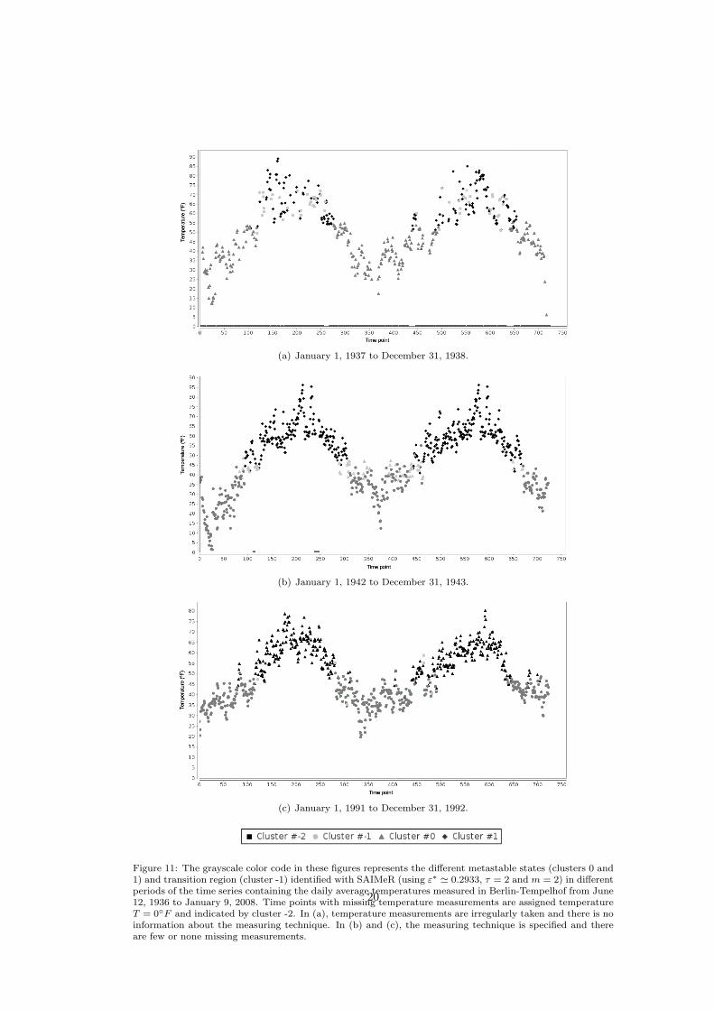
result of this analysis is shown in Fig. 11 (a).This period has several missing measurements – around 30% of the time points – and there

is no information about the way in which measurements were taken. In this time serieswe identify one metastable state corresponding to a colder season (cluster 0 in the figure),which lasts around six months. A second metastable state (cluster 1 in the figure) and

18

Figure 10: Merged time series. Obtained from the time series in Fig. 9 (containing the daily averagetemperatures in Berlin-Tempelhof measuring station from June 12, 1936 to January 9, 2008) by ignoring thetime points in which no measurements were taken.

the time points associated to the transition region (cluster -1 in the figure) do not seem tocorrespond to any yearly season. These results might originate from the large amount ofmissing measurement points in the time series, which would require a different recurrencethreshold and embedding dimensions to be analyzed. Another reason for these results mightbe the dispersion of the temperature measurements data, which might originate from a non-systematic measuring technique. A suggestion to improve the identification of metastablestates in this time series is to analyze it with different recurrence threshold and embeddingparameters, specific for these data and not for the coarse time series.

The second period of time we analyze goes from January 1, 1942 to December 31, 1943.The result of this analysis is shown in Fig. 11 (b).

This period does not have many missing measurements – less than 1% of the time points – .The temperature measureents data in this region are less disperse than in the previous region,which suggests a more systematic measuring technique. In this time series we identify onemetastable state (cluster 0 in the figure) corresponding to a colder season, which lasts aroundsix months, and another metastable states (cluster 1 in the figure) corresponding to a warmerseason that also lasts around six months. Cluster -1 indicates points in between the warmerand the colder seasons coming from the transition region in the final recurrence networkassociated to this period of measurements. Time points in cluster -1 relate to the periods oftransition between the colder and the warmer seasons.

The third period of time we analyze goes from January 1, 1991 to December 31, 1992.The result of this analysis is shown in Fig. 11 (c).

This period does not have missing measurements. Additionally, temperature data in thisregion were obtained with a more systematic measuring technique. In this time series weidentify one metastable state (cluster 0 in the figure) corresponding to a colder season, whichlasts around six months, and another metastable state (cluster 1 in the figure) correspondingto a warmer season that also lasts around six months. Cluster -1 indicates the periods oftransition between the colder and the warmer seasons.

To the best of our knowledge, the time series data analyzed in this section has not beenpreviously analyzed in any similar fashion. However statistical analysis and interpretationsof such analysis have been performed [42].

19

(a) January 1, 1937 to December 31, 1938.

(b) January 1, 1942 to December 31, 1943.

(c) January 1, 1991 to December 31, 1992.

Figure 11: The grayscale color code in these figures represents the different metastable states (clusters 0 and1) and transition region (cluster -1) identified with SAIMeR (using ε∗ ' 0.2933, τ = 2 and m = 2) in differentperiods of the time series containing the daily average temperatures measured in Berlin-Tempelhof from June12, 1936 to January 9, 2008. Time points with missing temperature measurements are assigned temperatureT = 0F and indicated by cluster -2. In (a), temperature measurements are irregularly taken and there is noinformation about the measuring technique. In (b) and (c), the measuring technique is specified and thereare few or none missing measurements.

20

5 Robustness

In this section we measure the robustness of SAIMeR. We define robustness as the similaritybetween the metastable states identified in a (original) time series and in the same timeseries when some artifacts have been added. By artifacts we understand noise or missingdata points.

We measure robustness with the Adjusted Rand Index [43] (ARI), developed by Hubertand Arabie in 1985. The ARI is a measurement of agreement between two (clustering)partitions that ranges from 0 – when the partitions are not similar at all – to 1 – when thepartitions are the same – . This can be used even if the number of clusters in the two partitionscompared is different, assigns a constant value of zero to the expected value of agreementbetween two random partitions and does not get affected when comparing partitions with ahigh number of clusters. The expression of this index can be found in Appendix B.

Since we use the MSM clustering algorithm in SAIMeR, we need to adapt the measure-ment of similarity in order to account for the different partition of the networks into modularand transition regions. This treatment is based on the work of Hueffner et al. from 2013 [11],in which every node identified as part of the transition region of a recurrence network isassigned to an independent cluster in order to create a full partition, in which the ARI iscomputed. In the following analysis, we will use this type of partitioning.

In our case, the two clustering partitions used to compute the ARI are the ones comingfrom the MSM clustering analysis of the final recurrence networks associated to a time seriesand the same time series with added artifacts.

We analyze the robustness of SAIMeR in two cases: when a time series has a percentageof noise added and when a percentage of time points has been removed from a time series.For these analysis, we take as example a double well potential time series.

5.1 Noisy time series

To test the robustness of SAIMeR to analyze time series with noise, we measure the simi-larity between (a) the clustering partition obtained from analyzing a time series and (b) theclustering partition obtained from analyzing a noisy time series. We compare two differenttypes of noisy time series, whose construction we describe below.

The results we show in the following two sections, suggest that SAIMeR is able to identifymetastable states in time series with noise of amplitude up to 20% the amplitude of theoriginal time series or with amplitude up to 200 times the minimum variation (different tozero) in consecutive measurement points in the time series.

Our results also confirm Zbilut’s statement of inflation of the embedding dimension whenreconstructing the state space from noisy time series [3]. Thus, the ARI is higher whenselecting different embedding parameters (as explained in Appendix A) to reconstruct thestate space from noisy time series.

5.1.1 Noise as a fraction of minimum change between consecutive measurementpoints

The first definition of noisy time series we use is the one indicated by Hassona [44] for theanalysis of variations of RQA measurements when adding noise to time series data. In this,a noisy time series is computed by adding Gaussian white noise (mean µ = 0 and standarddeviation σ = 1) with amplitude equal to a multiple, α, of the minimum variation differentto zero in consecutive measurement points to the time series. We vary the amplitude of noisefrom α = 1 to α = 100 in intervals ∆α = 10. For every increase in the amplitude of noise,

21

we compute 10 different time series, in order to get rid of the bias produced by the selectionof noise.

We simulate a time series for the double well potential, as described in Section 4.1, andanalyze it with SAIMeR. The recurrence threshold and the embedding parameters used inthis case are ε ' 0.3922, τ = 3 and m = 2.

Using the same recurrence threshold and embedding parameters for the construction ofthe state space associated to each noisy time series, we obtain the results shown in Fig. 12.In this plot, the ARI indicating the similarity between the original and the noisy partitionsis lower than 0.6 for α < 25.

Figure 12: Similarity, measured with the Adjusted Rand Index (ARI), between the metastable states identifiedin the original time series and in the time series where white Gaussian noise has been added. In this case, theamplitude of noise is equivalent to a fraction, α, of the minimum change between consecutive measurementpoints. All partitions are computed with the same recurrence threshold ε ' 0.3922 and embedding parametersτ = 3 and m = 2.

As mentioned by Zbilut in 1992 [3], having noise in a time series has an effect of inflationof the embedding dimension when reconstructing the state space. The low resistance tonoise shown in Fig. 12 could indicate the necessity to increase the embedding dimension aswe increase α. To confirm this suggestion, we perform a second experiment where everynoisy time series is analyzed with different recurrence threshold and embedding parameters.In this case we vary α from 1 to 200, in intervals ∆α = 10. The results we obtain are shownin Fig. 13.

As Figs. 12 and 13 suggest, adapting a recurrence threshold and embedding parametersto every noisy time series, increases the ARI measured with the noisy and the original timeseries. Without adapting the analysis parameters, ARI < 0.6 for α < 30, but adapting them,the ARI does not drop lower than 0.6 even for α equal to 200.

5.1.2 Noise as a percentage of the amplitude of the time series

The second definition of noisy time series we use also corresponds to the addition of Gaussianwhite noise to the time series (mean µ = 0 and standard deviation σ = 1), but with amplitudeequal to a percentage, α′, of the amplitude of the original time series. In this case, theamplitude of noise varies from α′ = 0 to α′ = 100 in intervals ∆α′ = 10. Once more, in order

22

Figure 13: Similarity, measured with the Adjusted Rand Index (ARI), between the metastable states identifiedin the original time series and in the time series where white Gaussian noise has been added. In this case, theamplitude of noise is equivalent to a fraction, α, of the minimum change between consecutive measurementpoints. Every partition is computed with different embedding parameters and recurrence thresholds. Therange of α is larger than in Fig. 12, showing that this approach provides more similar results (ARI > 0.6).

to get rid of the bias produced by the different noise introduced, we try 10 different noisytime series for every increase in the amplitude of noise analyze each of them with differentrecurrence threshold and embedding parameters.

We simulate a time series for the double well potential, as described in Section 4.1, andanalyze it with SAIMeR. According to the results obtained in Section 5.1.1, the recurrencethreshold and embedding parameters we use are different for every noisy time series analyzed.In Fig. 14 we observe the similarity in clustering results between (a) the noisy and (b) theoriginal time series.

The ARI measuring the similarity between the clustering partitions for the noisy and forthe original time series, is higher than 0.6 for α′ ≤ 20. ARI values remain higher than 0.9for α′ ≤ 10.

These results suggest that, when adapting a recurrence threshold and embedding param-eters to every noisy time series, SAIMeR enables the identification of metastable states in thesystem even for time series with noise with amplitude given by α = 20, or 20% the amplitudeof the original time series.

5.2 Removing data points

One of the typical features of real-world time series is having observations irregularly taken.This irregularity can be understood as if a percentage of measurement points, randomlydistributed in the time series, had been removed from a time series containing a set ofmeasurements regularly taken.

To analyze this type of irregular time series, we produce a time series with regularlyspaced measurements, called the original time series, and assign to a percentage of randomlydistributed data points a “null” value. We refer to the time series resulting from this processas the trimmed time series. Since we are not ignoring time points but only assigning a newvalue to some time points, the length of the original and the trimmed time series is the same.

23

Figure 14: Similarity, measured with the Adjusted Rand Index (ARI), between the metastable states identifiedin the original time series and in the time series where white Gaussian noise has been added. In this case,the amplitude of noise is equivalent to a percentage α′ of the amplitude of the original time series. Everypartition is computed with different embedding parameters and recurrence thresholds.

We vary the percentage of time points being removed from 0% to 19%, in intervals of 1%.For every percentage of data points being removed, we compute 10 different time series, inorder to get rid of the bias produced by the selection of data points to remove.

We compare the partition obtained by analyzing the original time series and the partitionobtained by analyzing the trimmed time series.

All the clustering partitions associated to the trimmed time series are computed using thesame recurrence threshold originally computed with the complete time series, ε ' 0.3678.

However, we interpret the case of removing measurement points from the time series asanother case of noise and therefore we use different embedding parameters for the reconstruc-tion of the the state space from every time series with artifacts. Every recurrence networkassociated to a trimmed time series is computed with different embedding parameters. Fig. 15shows the ARI values obtained.

In Fig. 15 we see that the ARI has values higher than 0.9 for time series with up to 5%of time points removed. The ARI does not have values lower to 0.6 even for time series withup to 19% of time points being removed. These results suggest that the recurrence thresholdcomputed with SAIMeR enables the identification of the metastable states even for timeseries with up to 19% of randomly distributed missing points.

We believe that these results could be improved by selecting a different recurrence thresh-old for every time series with missing points with which the comparison is performed. How-ever, since the results obtained by using the same recurrence threshold already allow a goodidentification of the metastable states, we maintained this methodology due to its simplicity.

24

Figure 15: Similarity, measured with the Adjusted Rand Index (ARI), between the metastable states identifiedin the original time series and the trimmed time series, which contains a percentage of randomly distributedmissing data points. All partitions are computed with different embedding parameters but with the samerecurrence threshold ε ' 0.3678.

6 Conclusions

In this paper, we present SAIMeR, a self-adapted method for the identification of metastablestates in real-world time series based on recurrence networks analysis.

SAIMeR uses particular statistical information of the time series analyzed in order to pro-duce a recurrence threshold. Clustering the recurrence network associated to such recurrencethreshold results in the classification of time points into different metastable states.

We use three examples to illustrate the performance of SAIMeR, where we identifymetastable states that correspond to the different dynamical behaviors in such time series.The first example is a double well potential, where we identify two metastable states, whichcorrespond to moments in which the simulated particle is in each of the potential wells, plusa region of transition between such states. The second example is the molecular confor-mations of trialanine. We identify five main metastable states in this data, which seem tocorrespond to the different conformation states of the molecule mentioned by Fischer et al.in 2006 [38]. The third example corresponds to the daily average temperature measured inBerlin-Tempelhof between June 12, 1936, and January 9, 2008. In this time series, despitethe several missing data points in some regions of the time series, we identify two mainmetastable states, corresponding to the warmer and the colder seasons.

Additionally, we show that SAIMeR gives similar results (measured with the AdjustedRand Index [43] [ARI]) when identifying metastable states on time series with artifacts (wherenoise have been added or data points have been removed). Similarity is measured for timeseries where a percentage of data measurements have been removed, where ARI > 0.6 evenfor time series with 19% of data points removed. It is also measured for time series withGaussian white noise added. We consider two definitions of noise. In the first, the amplitudeof noise is expressed as a multiple, α, of the minimum variation different to zero betweenconsecutive measurements in the time series. In this case, ARI is higher than 0.6 even forα = 200. In the second definition, the amplitude of noise is expressed as a percentage, α′,

25

of the amplitude of the original time series. In this case, ARI is higher than 0.6 even forα′ = 20.

Finally, since any recurrence analysis requires the reconstruction of the state space andsince we use the delay mapping for this purpose, we propose a methodology to determineappropriate embedding parameters (delay and dimension). We propose that the embeddingparameters must provide the first minimum of entropy and maximum of recurrence rate dur-ing the recurrence analysis of the time series with SAIMeR. The selection of these parameters,prior to the recurrence analysis, is still an open problem that we aim to approach in futurework.

All the results of the experiments mentioned above suggest that SAIMeR is an efficienttool for the analysis of real-world time series.

A Comments about Taken’s embedding parameters.

Recurrence quantitative analysis (RQA) measurements are sensitive to variations in the re-currence threshold and embedding parameters. Here, we analyze the sensitivity of two quan-titative measurements when varying the embedding parameters for SAIMeR on the doublewell potential time series in Fig 4: the entropy (Eq. 12) and the recurrence rate (Eq. 11).

A.1 Recurrence rate

The recurrence rate [3, 45], RR, is a recurrence measurement that indicates the percentageof recurrence points in a recurrence plot. In terms of the recurrence network, it indicatesthe relative frequency of edges a node contributes to [24]. This way, higher values in thismeasurement indicate that the nodes are more connected. Or, in other words, that a largernumber of state space vectors are inside a same state space neighborhood.

RR =1N2

N∑i,j=1

Rij(ε∗) (11)

A.2 Entropy

Entropy, S(ε∗), refers to the Shannon entropy and indicates the probability to find a diagonalline of length l in a recurrence plot Rij(ε∗). In other words, it indicates the complexityof a recurrence plot, with respect to its diagonal lines. As a recurrence plot depends onthe recurrence threshold, variations in this parameter will modify the value of the entropy.Variations in the embedding parameters will also modify this value [46].

Being Rij(ε∗) a recurrence plot computed from N∗ state space vectors and P (l) = P (ε∗, l)its histogram of diagonal lines of length l, the relative frequency of diagonal lines with lengthl is given by p(l) = P (l)/Nl. This relative frequency is equal to the number of diagonal lineswith length l divided by the total number of state space vectors. This way, according toMarwan et al. [16], entropy is given by:

S = −N∗∑lmin

p(l) log p(l) (12)

In Eq. 12, lmin is the minimum length of the diagonal lines in a recurrence plot. Thislength can be defined for a recurrence plot computed from non-noisy time series. However,we want to work with real-world time series data and expect to have noise.

26

According to Marwan et al. [16], entropy is small for recurrence plots computed fromnoisy time series. This is expected because noisy time series produce recurrence plots withmany short and thin diagonal lines and single points. Since we wand to distinguish noise fromthe rest of our time series data, we would like to remove short diagonals from the entropycomputation. Therefore, we compute a new minimum length of the diagonal lines, l∗min, as:

l∗min =∑N∗

l=0 lp(l)∑l=0 p(l)

(13)

In general, a lower value in entropy indicates that a recurrence plot has thinner diagonallines, which in turn indicates less time intervals with similar evolution in the time seriesoriginating such recurrence plot. This way, a minima in entropy could indicate the recoveryof more dynamical structure in the associated recurrence plot. For this reason, we would liketo find a recurrence threshold and embedding parameters that produce recurrence plots witha lower value of entropy.

A.3 Embedding parameters

We suggest that selecting the embedding parameters that first provide a simultaneous lo-cal minima in entropy and local maxima in recurrence rate, and that also give the lowestminimum in entropy, construct a state space in which more nodes are closer for smallerneighborhoods. This kind of space would provide more structure in the associated recur-rence networks produced when analyzing recurrences in the state space.

To illustrate our suggestion, we use the time series for a double well potential. Determininga selection of embedding delay and embedding dimension, we can construct the state spaceassociated to this time series and compute a final recurrence threshold. With this recurrencethreshold and the state space constructed with the selected embedding parameters, we cancompute the recurrence plot associated to the time series. In this recurrence plot we measurethe recurrence rate and the entropy.

Graphs in Fig. 16 show the different recurrence rate and entropy values obtained fordifferent selections of embedding parameters when analyzing a double well potential timeseries. Embedding parameters that first provide a simultaneous local minima in entropy andlocal maxima in recurrence rate, are pointed in circles. From these combination, we selectthose that produce the recurrence plot with minimum entropy and use them in SAIMeR inorder to identify metastable states.

B The Adjusted Rand index

This index measures the agreement between any two (clustering) partitions, even if thenumber of clusters in each of them is different. It assigns a constant value of zero to theexpected value of agreement between two random partitions and ranges between zero andone.

Let us imagine S = O1, ..., ON, a set of objects. The number of combinations of pairsthat are possible to make from set S is

(N2

). Set P = p1, p2, ..., pA and Q = q1, q2, ..., qB

two partitions (or collections of subsets) of S such that ∪Aa=1pa = ∪Bb=1qb = S, pa ∩ pa′ = ∅for any a 6= a′, and qb ∩ qb′ = ∅ for any b 6= b′. If tab represents the number of objects inS that were classified in the a-th subset of P and in the b-th subset of Q, then the ARI, as

27

(a) Entropy (b) Recurrence rate

Figure 16: Plot showing the variation in the entropy (computed as in Eq. 12) and recurrence rate (computedas in Eq. 11) for the different recurrence plots associated to the same time series of a double well potentialresulting from constructing different state spaces with different embedding parameters (embedding delay anddimension). The circles in the plot point at the combination of embedding dimension and delay for which wefind a simultaneous local minimum in entropy and a first local maximum in recurrence rate.

defined by Santos [47], can be expressed as the quotient F1/F2, where:

F1 =(n

2

) A∑a=1

B∑b=1

(tab2

)−

A∑a=1

(ta·2

) B∑b=1

(t·b2

)

F2 =12

(n

2

)[ A∑a=1

(ta·2

)+

B∑b=1

(t·b2

)]−

A∑a=1

(ta·2

) B∑b=1

(t·b2

)

C Sankey diagram for two well potential time seriesanalysis.

Sankey diagrams are a visual tool that shows the number of clusters as well as the nodesdistribution for each of the different recurrence networks computed from the tuning set εν.

In these diagrams, each network is represented as a column, the number of clusters in anetwork is represented as sections of the column whose size corresponds to the number ofnodes each cluster has. The amount of nodes whose correspondence to a cluster varies fromone network to another, is represented as a flux between columns, and the width of such fluxcorresponds to the number of nodes whose classification differs between two networks.

Fig. 17 shows the Sankey diagram used for the two well potential time series analysis ofSection 4.1. In this particular diagram, we observe a group of networks (columns) with thesame number of clusters (size of sections of a column), for which the number of nodes in eachcluster is almost the same (low flux of nodes from one column to another). This is the setof networks with which we compute the final recurrence threshold used for the identificationof metastable states in the two well potential time series. Recurrence networks fulfillingconditions 6 and 7, have a similar number and size of clusters identified. We suggest that

28

these networks define a set of recurrence thresholds giving robust results about the dynamicsof the time series analyzed.

Figure 17: Sankey diagram showing the subgroup of recurrence networks (columns) with the same numberof clusters (see eq. 6) and similar number of nodes (see eq. 7). Networks are computed from tuning set εν(see eq. 5) on the state space constructed from a two well potential time series and embedding parametersτ = 7 and m = 2. We suggest that this group of networks determines the recurrence threshold giving robustresults about the dynamics of the time series analyzed.

D Weather data: Specifications

The time series mentioned in Section 4.3 has several periods of time without temperaturemeasurements. Before August 31, 1939 measurements are irregular. After that day, temper-ature is taken daily, even though the measuring technique is not specified. Measurementscontinue until December 31, 1943, after a short interruption from August 29, 1942 to Septem-ber 5, 1942.

During the three decades after December 31, 1943 There are no measurements. Anexception are the seven months from February 1, 1949, to August 27, 1949. These decadesinclude the end of the war, on 1945 and the Cold War.

Measurements start again on January 1, 1973 and are uninterrupted until December 31,1992. However, after that date, measurements are scarce. Temperature was measured in 2003only from May 18 to June 28, and from August 10 to August 16. During 2005, temperaturewas measured from May 16 to May 31. The last measurements we consider in our analysiswere taken from December 3, 2007 to January 9, 2008.

29

References

[1] L. van der Maaten, E. Postma, and J. van den Herik. Dimensionality Reduction: AComparative Review. Tilburg University, Netherlands, 2009.

[2] S. O. Kamphorst J. P. Eckmann and D. Ruelle. Recurrence plots of dynamic-systems.Europhysics Letters, 4(9):973–977, 1987.

[3] J. P. Zbilut and C. L. Webber Jr. Embeddings and delays as derived from quantificationof recurrence plots. Physics Letters A, 171:199–203, 1992.

[4] J.P. Zbilut A. Krishnan, A. Giuliani and M. Tomitah. Implications from a network-basedtopological analysis of ubiquitin unfolding simulations. PLoS ONE, 3, 2008.

[5] M. Tomita A. Krishnan, J.P. Zbilut and A. Giuliani. Proteins as networks: usefulnessof graph theory in protein science. Curr. Prot. Peptide Sci., 9:28–38, 2008.

[6] Jonathan F. Donges, Jobst Heitzig, Reik V. Donner, and Jurgen Kurths. Analyticalframework for recurrence network analysis of time series. Phys. Rev. E, 85:046105, Apr2012.

[7] Reik V. Donner, Yong Zou, Jonathan F. Donges, Norbert Marwan, and Jurgen Kurths.Ambiguities in recurrence-based complex network representations of time series. Phys.Rev. E, 81:015101, Jan 2010.

[8] O. Dimigen S. Schinkel and N. Marwan. Selection of the recurrence threshold for signaldetection. The European Phys. J., 164:45–53, 2011. Special Topics.

[9] M. Sarich et al. Modularity revisited: A novel dynamics-based concept for decomposingcomplex networks. To Appear, Journal of Computational Dynamics, 2012. http://publications.mi.fu-berlin.de/1127/.2,3,5.

[10] M. Sarich and C. Schuette. Approximating selected non-dominant timescales by markovstate models. Comm. Math. Sci., 10(3):1001–1013, 2012.

[11] S. Hueffner, B. Kayser, and T. O. F. Conrad. Finding modules in networks with non-modular regions. Lecture Notes in Computer Science, 7933:188–199, 2013. Proceedingsof the 12th international symposium, SEA 2013.

[12] N. Djurdjevac, S. Bruckner, T. O. F. Conrad, and C. Schuette. Random walks on com-plex modular networks. Journal of Numerical Analysis Industrial and Applied Mathe-matics, 6(1-2):29–50, 2012.

[13] H. Poincare. Sur le probeeme des trois corps et les ´quations de la dynamique. ActaMathematica, 13(1-270), 1890.

[14] M. Thiel N. Marwan, M. C. Romano and J. Kurths. Crossed recurrence plot basedsynchronization of time series. Nonlinear Processes in Geophysics, 9:325–331, 2002.

[15] Norbert Marwan, Niels Wessel, Udo Meyerfeldt, Alexander Schirdewan, and JurgenKurths. Recurrence-plot-based measures of complexity and their application to heart-rate-variability data. Phys. Rev. E, 66:026702, Aug 2002.

[16] M. Thiel N. Marwan, M. C. Romano and J. Kurths. Recurrence plots for the analysisof complex systems. Physics Reports, 438:237–329, 2007.

30

[17] N. Marwan et al. Complex network approach for recurrence analysis of time-series. Phys.Letters A, 373:4246–4254, 2009.

[18] J. A. Yorke T. Sauer and M. Casdagli. Embedology. J. Stat. Phys., 65(3-4):579–616,1991.

[19] F. Takens. Detecting strange attractor in turbulence, volume 898 of Lecture Notes inMathematics. Springer Verlag, Berlin, 1981.

[20] H. Whitney. Differentiable manifolds. Ann. Math., 37:645–680, 1936.

[21] H. D. I. Abarbanel. Analysis of Observed Chaotic Data. Springer Verlag, Berlin, 1996.

[22] C. Letellier, I. M. Moroz, and R. Gilmore. Comparison of tests for embeddings. Phys.Rev. E, 78:026203, Aug 2008.

[23] R. V. Donner et al. Recurrence networks a novel paradigm for nonlinear time-series anal-ysis. New Journal of Physics, 12:033025, 2010. DOI:10.1088/1367-2630/12/3/033025.

[24] R. V. Donner et al. The geometry of chaotic dynamics - a complex network perspective.Eur. Phys. J. B, 2011. DOI:10.1140/epjb/e2011-10899-1.

[25] Y. Zou et al. Identifying complex periodic windows in continuous-time dy-namical systems using recurrence-based methods. CHAOS, 20:043130, 2010.DOI:10.1063/1.3523304.

[26] P. Grassberger and I. Procaccia. Measuring the strangeness of strange attractors. PhysicaD, 9(1-2):189–208, 1983.

[27] P. L. Read M. Thiel, M. C. Romano and J. Kurths. Estimation of dynamical invariantswithout embedding by recurrence plots. CHAOS, 14(2):234–243, 2004.

[28] N. Marwan A. P. Schutz, Y. Zou and M. T. Turvey. Local minima-based recurrence plotsfor continuous dynamical systems. Int. J. Bifurcation and Chaos, 21(4):1065–1075, 2011.DOI: 10.1142/S0218127411029045.

[29] Jesper Dall and Michael Christensen. Random geometric graphs. Phys. Rev. E,66:016121, Jul 2002.

[30] M. Penrose. Random Geometric Graphs. Oxford University Press, Oxford, 2003.

[31] T. Hsing and H. Rootzen. Extremes on trees. Ann. Probab., 33(1):413–444, 2005.

[32] C. Cooper and A. Frieze. Component structure of the vacant set induced by a randomwalk on a random graph. Random Structures and Algorithms, 42(2):135–158, 2013.DOI:10.1002/rsa.20402.

[33] Z. Kong and E. M. Yeh. On the critical density for percolation in random geometricgraphs. Proceedings of IEEE International Symposium on Information Theory, ISIT2007, 1-7:151–155, 2007. DOI:10.1109/ISIT.2007.4557082.

[34] H. A. Kramers. Brownian motion in a field of force and the diffusion model of chemicalreactions. Physica, 7:284–304, 1949.

[35] R. Preis et al. Dominant paths between almost invariant sets of dynamical systems.2004. preprint available in http://www.biocomputing-berlin.de/biocomputing/en/?cmd=publication.

31

[36] L. Putzig P. Metzner and I. Horenko. Analysis of persistent non-stationary time seriesand applications. CAMCoS, 7(2):175229, 2012. DOI: 10.2140/camcos.2012.7.1753.

[37] M. Munz and P. C. Biggin. Jgromacs: a java package for analyzing protein simulations.J. Chem. Inf. Model, pages 255–259, 2012.

[38] A. Fischer et al. Identification of biomolecular conformations from incomplete torsionangle observations by hidden markov models. J. Comput. Chem., 28:2453–2464, 2006.DOI: 10.1002/jcc.20692.

[39] Rimfrost database. http://www.rimfrost.no/.

[40] Deutscher wetterdienst. http://www.dwd.de/.

[41] Nasa goddard institute for space studies. http://data.giss.nasa.gov/gistemp.

[42] Data base: Urban and environmental information system (ueis) berlin department forurban development and the environment. http://www.stadtentwicklung.berlin.de/umwelt/umweltatlas/ed412_03_zusatz.htm.

[43] L. Hubert and P. Arabie. Comparing partitions. Journal of Classication, 2:193–218,1985.

[44] C. J. Hassona. Influence of embedding parameters and noise in center of pressure recur-rence quantification analysis. Gait and Posture, 27(3):416–422, 2008.

[45] C. L. Webber Jr. and J. P. Zbilut. Recurrence quantification analysis of nonlineardynamical systems. Tutorials in contemporary Nonlinear Methods for the BehavioralSciences Web Book. Riley, National Science Foundation US, 1995.

[46] P. Faure and H. Korn. A new method to estimate the kolmogorov entropy from recur-rence plots: its application to neuronal signals. Physica D, 122:265–279, 1998.

[47] J. M. Santos and M. Embrechts. On the use of adjusted rand index as a metric forevaluating supervised classification. Proceedings of the 19th International Conferenceon Artificial Neural Networks: Part II, pages 175–184, 2009.

[48] J. M. Hammersleyh. The distribution of distance in a hypersphere. Ann. Math. Statist.,21:447–452, 1950.

[49] O. Amidi S. Toal and R. Schweitzer-Stenner. Conformational changes of trialanineinduced by direct interactions between alanine residues and alcohols in binary mixturesof water with gycerol and ethanol. J. Am. Chem. Soc., 133:12728–12739, 2011. DOI:10.1021/ja204123g.

[50] Y. Xu M. (I-Hsien) Tsai and J. J. Dannenberg. Ramachandran revisited. DFT energysurfaces of diastereomic trialanine peptides in the gas phase and aqueous solution. J.Phys. Chem. B, 113:309–318, 2009.

32