Embed Size (px)
Citation preview

Insights into metastability of photovoltaic materials at the mesoscale through massiveI–V analyticsTimothy J. Peshek, Justin S. Fada, Yang Hu, Yifan Xu, Mohamed A. Elsaeiti, Erdmut Schnabel, Michael Köhl,and Roger H. French Citation: Journal of Vacuum Science & Technology B 34, 050801 (2016); doi: 10.1116/1.4960628 View online: http://dx.doi.org/10.1116/1.4960628 View Table of Contents: http://scitation.aip.org/content/avs/journal/jvstb/34/5?ver=pdfcov Published by the AVS: Science & Technology of Materials, Interfaces, and Processing Articles you may be interested in Dense nanoimprinted silicon nanowire arrays with passivated axial p-i-n junctions for photovoltaic applications J. Appl. Phys. 117, 125104 (2015); 10.1063/1.4916535 Photovoltaic characteristics of amorphous silicon solar cells using boron doped tetrahedral amorphous carbonfilms as p -type window materials Appl. Phys. Lett. 90, 083508 (2007); 10.1063/1.2539767 Metastable defect migration under high carrier injection in hydrogenated amorphous silicon p - i - n solar cells J. Appl. Phys. 98, 044511 (2005); 10.1063/1.2010623 The open circuit voltage in amorphous silicon p - i - n solar cells and its relationship to material, device and darkdiode parameters J. Appl. Phys. 96, 2261 (2004); 10.1063/1.1769092 Method to extract diffusion length from solar cell parameters—Application to polycrystalline silicon J. Appl. Phys. 93, 5447 (2003); 10.1063/1.1565676
Redistribution subject to AVS license or copyright; see http://scitation.aip.org/termsconditions. IP: 129.22.124.78 On: Fri, 12 Aug 2016 20:32:53

REVIEW ARTICLE
Insights into metastability of photovoltaic materials at the mesoscalethrough massive I–V analytics
Timothy J. Peshek,a) Justin S. Fada, Yang Hu, Yifan Xu, and Mohamed A. ElsaeitiDepartment of Materials Science and Engineering, Case Western Reserve University, Cleveland, Ohio 44106
Erdmut Schnabel and Michael K€ohlFraunhofer Institute for Solar Energy Systems (ISE), Heidenhofstrasse 2, 79110 Freiburg, Germany
Roger H. FrenchDepartment of Materials Science and Engineering, Case Western Reserve University, Cleveland, Ohio 44106
(Received 3 May 2016; accepted 26 July 2016; published 12 August 2016)
The authors demonstrate the feasibility of quantifying cell-level performance heterogeneity from
module-level I–V curves by determining conditions of bypass diode turn-on. Analysis of these
curves falls outside of typical diode-based models of photovoltaic (PV) performance. The authors
show that this approach can leverage statistical and machine learning techniques for broad applica-
tion to massive datasets, and combine those insights with simulations and laboratory-based experi-
ments to provide useful information into the metastability of the interfaces of a PV cell. The
authors find good agreement between the experimentally determined curves and the simulated
curves, which guide the variable selection in the massive dataset collected from sites in Cleveland,
OH, USA, the Negev Desert, Israel, Isla Gran Canaria, Spain, and Mount Zugspitze, Germany.VC 2016 Author(s). All article content, except where otherwise noted, is licensed under a CreativeCommons Attribution (CC BY) license (http://creativecommons.org/licenses/by/4.0/).[http://dx.doi.org/10.1116/1.4960628]
I. INTRODUCTION AND BACKGROUND
The study of real materials systems undergoing real-world
operation and degradation processes is a challenging problem
in the area of mesoscale science.1–3 We focus here on the tem-
poral evolution of electrical properties and behavior of photo-
voltaic energy materials, particularly crystalline silicon solar
cells, which include dynamics on timescales from minority
carrier lifetimes in milliseconds to degradation-related device
lifetimes in gigaseconds (30 years).4 Connection across this
broad expanse of time-scales is essential for a physics-based
understanding of slow and rare events associated with degra-
dation and performance over lifetime. We provide a review
of literature relating to the topics of modeling the current–
voltage characteristics (I–V curves) of solar cells and modules
and the challenges of connecting those performance models
to both large scale deployment of photovoltaics and action-
able insights into the microscopic performance mechanisms.
With the rapid deployment of large scale global photovol-
taics, there exist massive time-series datastreams on perfor-
mance that can be aggregated and mined for signatures of
climate-dependent degradation. In this sense, a statistically
or data-driven approach to modeling the performance can
detect subtle population differences and indicate the impact
of real-world dynamics on the system metastability and per-
formance. The laboratory and its analytical tools remains the
arena where macroscopic performance can be linked to
mesoscopic behavior; yet correlating any “engineered
damage” to the solar cells to real-world performance remains
a high barrier. This barrier is greatly reduced through
acquiring and mining complete current–voltage (I–V) and
maximum power point (Pmp) characteristics as time-series
datastreams on cells in these two arenas and by acquiring
massive data on the real-world environment using distributed
sensors and newer forms of satellite-based imagery for
weather and insolation data. Degradation-induced failures
have been an ongoing characteristic of new and promising
PV cells5 and other energy materials even as producers con-
tinue to offer 25 year warranties.
We will first discuss the dominant physics-based diode
models that have been used to extract useful parametric
information on photovoltaic cell performance. Next we dis-
cuss the realistic electrically active interfaces in typical crys-
talline silicon cells, and how these encompass a more
complex device architecture than a simple diode model
approach. Various methods are then presented for extracting
useful information from I � V;Pmp time-series, comparing
and contrasting the physics-based approaches with different
data-driven statistical and machine learning approaches.
This I � V;Pmp time-series analysis approach is then demon-
strated by developing lab-based hypotheses and experiments
that are compared quantitatively with observed real-world
data, and generating a data-driven hypothesis-testing processa)Electronic mail: [email protected]
050801-1 J. Vac. Sci. Technol. B 34(5), Sep/Oct 2016 2166-2746/2016/34(5)/050801/11 VC Author(s) 2016. 050801-1
Redistribution subject to AVS license or copyright; see http://scitation.aip.org/termsconditions. IP: 129.22.124.78 On: Fri, 12 Aug 2016 20:32:53

model, so as to illustrate some of the opportunities of this
approach.
A. Physics-based diode models for photovoltaic cells
To model the I–V curve of an arbitrary solar cell a macro-
scopic physics-based model consisting of a current source,
single pn diode, and two resistors is typically utilized.6
Often, researchers may also add a parallel second diode, or
“recombination diode” that describes an internal carrier
recombination process that is nonlinear.7,8 In this “two-
diode” model solving parallel Shockley equations becomes
intractable and many assumptions are required to simplify
and specify the system.9 For simplicity, many researchers
study performance within the paradigm of the single diode
model. This model has had good success reproducing the
shape of the curve for single cells, but its coarse grain struc-
ture yields few insights into mesoscopic behavior. To illus-
trate this issue, we describe a typical approach to obtain the
series resistance of a solar cell, which typically represents
the behavior of the front and back cell contacts.
Applying Kirchoff’s laws and the Shockley equation
yields the relationship between current (I) and voltage (V)
for a solar cell in this single-diode model
I V; Tð Þ ¼ IL � I0 expV þ IRS
NsnVth Tð Þ � 1
� �� V þ IRS
Rsh; (1)
where IL is the light induced current from photon absorption,
I0 is the reverse saturation current, Ns is the number of cells
in the module, n is the diode ideality factor, Rs is the cell
series resistance, Rsh is the cell shunt resistance, and Vth is
the thermal voltage equal to q/kT, where q is the elementary
charge of an electron and k is Boltzmann’s constant.
Because of the transcendental nature of Eq. (1), it is not pos-
sible to solve in terms of I(V) explicitly, except by means of
the Lambert-W function.10 Typically, these data may be
used simply to estimate Isc; Voc, maximum power point
(Pmp), fill factor (FF).
Many techniques for I–V curve parameter extraction
exist, ranging from simple to complex.11–20 All of these
techniques are based upon analyzing the transcendental
equation in certain regimes, i.e., near short circuit, open
circuit or maximum power, and drawing upon several
assumptions that typically hold for efficient solar cells. We
consider only methods that invoke the diode equation of
Eq. (1) and do not simplify it by, for example, ignoring the
shunt resistance contribution,20 and provide an example
analysis.15 We intend to determine the series resistance,
shunt resistance, and ideality factor variation in time. One
common and straightforward manner for estimating the
series and shunt resistance of the PV module is by simply
calculating the pointwise resistance curve for an I–V curve,
given by R(V)¼�1/(dI/dV), where Rs¼R(V¼Voc) and
Rsh ¼ RðV ¼ 0Þ.12
Analytical solutions to the transcendental equation exist
based upon the Lambert-W function,10,21 that Ghani et al.22
used to estimate the series, shunt resistances, and diode ide-
ality factor. This analytical solution for I(V, T) is given by
I V;Tð Þ ¼ IL � I0ð Þ �NsV=Rsh
1þRs=Rsh� nVth
Rs�W F V;Tð Þ½ �; (2)
where W[F(V, T)] is Lambert’s W function, with F(V, T), the
functional, equaling
F V;Tð Þ ¼ I0Rs
nVth RsþRshð Þ
� expNsV
nVth1� Rs
RsþRsh
� �þ IL � I0ð ÞRs
nVth RsþRshð Þ
� �:
(3)
This unwieldy analytical solution is straightforward to sim-
plify by invoking that generally Rsh � Rs and IL � I0; how-
ever, there is often more utility in solving for voltage, which
we will utilize later in Sec. III B:
V I; Tð Þ ¼ IL þ I0ð ÞRsh � I Rs þ Rshð Þ
�nVthWI0Rsh
nVthexp
IL þ I0 � Ið ÞRsh
nVth
� �� �: (4)
Petrone et al.23 found the analytical solution useful to pre-
dict behavior of a nonuniformly illuminated field of PV
modules, and researchers in the area of PV-related power
electronics have used the analytical solutions for maximum-
power-point-tracking algorithm development. However,
these methods are ultimately based upon the simplistic diode
equivalent circuit model that may not capture all of the
behavior of complex systems.
Although problems arise when using this technique, since
realistic values of Rs are only found when Rs is rather high,
compared to Rs of many real modules, and therefore, Rs
losses dominate the I–V curve as V approaches Voc. This
method for estimating Rsh is commonly used in many param-
eter extraction techniques15 although Hansen14 has ques-
tioned its validity and developed a novel iterative integral
approach to solving Eq. (1).
Khan15 found the slope of the I–V curve (m ¼ dI=dV),
and find moc and msc, which is dI=dV at V¼Voc and V¼ 0,
respectively,
msc ¼1=Rsh þ
I0Vth
nexp
IscRs
Vthn
� �� �
1þ Rs 1=Rsh þI0Vth
nexp
IscRs
Vthn
� �� � ; (5)
and
moc ¼1=Rsh þ
I0Vth
nexp
Voc
Vthn
� �� �
1þ Rs 1=Rsh þI0Vth
nexp
Voc
Vthn
� �� � : (6)
Under the assumptions
Rs � Rsh; (7)
Voc � IscRs; (8)
050801-2 Peshek et al.: Insights into metastability of photovoltaic materials 050801-2
J. Vac. Sci. Technol. B, Vol. 34, No. 5, Sep/Oct 2016
Redistribution subject to AVS license or copyright; see http://scitation.aip.org/termsconditions. IP: 129.22.124.78 On: Fri, 12 Aug 2016 20:32:53

which lead to the following inequality:
I0
Vthnexp
IscRs
Vthn
� �� 1
Rsh� I0
Vthnexp
Voc
Vthn
� �: (9)
Relation (9) allows for simplification of Eqs. (5) and (6), and
applying the substitution
I0 expVoc
Vthn
� �� Isc �
Voc
Rsh(10)
results in
m�1sc ¼ Rsh; (11)
m�1oc ¼ Rs þ nVth
1
Isc � Voc=Rsh
� �: (12)
Therefore, for a collection of I–V curves, the inverted slope
at open circuit has a linear dependence on 1=ðIsc � Voc=RshÞ,where the y-intercept is equal to Rs and the ideality factor
n can be obtained from the slope. This relation was tested
using massive real-world data,24 and we found that the
assumptions listed above held for typical PV modules.
Further we tested the model using nonuniformly illuminated
I–V curves, under mirror augmentation to seek signatures of
degradation and no significant change in the Rs was found
over 6 months. However, this analysis exhibited a bimodal
distribution in the estimation of Rs and overall indicated that
the method is not sensitive enough to track small changes in
the modules over this period of time. In addition, the assump-
tion that a 60-cell module is fully described by a single diode
model and particularly that a nonuniformly illuminated mod-
ule is described by a single shunt resistance is unreasonable.
In explorations beyond simplistic diode models, Sellner
et al.25,26 described a novel “loss factors model” that describes
six parameters that describe the system power losses and can
be more easily extracted from I–V curves. In the study of deg-
radation in performance, a loss factors model is a potentially
useful description of system performance; yet, this model is
largely derived from the diode model as well.27 As such,
the loss factors model cannot model and estimate or predict
behavior of I–V curves with bypass diodes.
II. MESOSCALE DESCRIPTION OF SOLAR CELLINTERFACES AND CONTACTS
Here, we focus on conventional Al back surface field
(BSF) solar cells which contain a series of distinct and criti-
cally important interfaces which play an essential role in the
performance and degradation of PV modules over their life-
time. It is common that engineering solutions to performance
issues are developed and commercialized without a complete
understanding of the behavioral mechanisms at the micro-
scale, let alone the lifetime limiting mechanisms towards
gigasecond time scales. These interfaces include the screen-
printed silver (SP-Ag) metallization grid, the front-surface
passivation, the pn junction itself, and the back-surface field
that limits recombination in the aluminum back-surface con-
tact. For example, the screen-printed silver metallization
grid on the front of the solar cells, which is applied as a paste
consisting of silver nanoparticles, glass frit, various organic
binders and subsequently fired, can be susceptible to corro-
sion from acetic acid produced in the ethylene-vinyl acetate
(EVA) encapsulant in front of the c-Si cell.
SP-Ag conductive lines are used in commercial silicon
photovoltaic (PV) cells as a front-side electrical contact to
the emitter. Formulation of the SP-Ag pastes includes
micron-scale silver particles (1–10 lm), glass, and organic
surfactants that facilitate printing and agglomeration upon
firing.28 The screen-printed precursor undergoes a firing pro-
cess that reaches up to 850 �C, where the glass frit etches the
SiNx antireflection coating allowing for contact formation to
the emitter. The final conductive lines are composed of
flocced silver particles and glass matrix.29,30 The geometry,
morphology, and components of the conductive lines have
been studied to minimize shading of the cells while main-
taining good conductance.31–33 Research on the conductive
lines has typically focused on the conductor line microstruc-
ture throughout the firing process34 and the interface
between the screen-printed conductive lines and the emitter
as a function of precursor constituents to optimize the initial
electrical performance.30,34–38 The microscopic mechanisms
that result in the formation of the low resistance contact
between the silver conductive lines and the solar cell are still
being uncovered,28 but two prevailing models are generally
accepted. One hypothesis suggests that the Ag becomes dis-
solved within the molten glass frit, and upon cooling down,
the supersaturated solution allows large grain growth at the
Si interface causing a Schottky-barrierlike boundary that
acts more Ohmic as the emitter doping concentration is
increased to nþþ levels. Another hypothesis is that Ag nano-
particles precipitate and are held in a colloidal suspension in
an interfacial glass film contacting the emitter, with conduc-
tion enabled through quantum mechanical tunneling through
the insulator regions. Cooper et al.28 investigated these mod-
els finding evidence for both models prevailing in various
regimes of firing temperature and emitter doping concentra-
tion; due to this dependency, one can expect that deployed
systems are widely varying and their response to climatic
conditions and degradation in performance is highly variable
and heterogeneous. We expect to see great variability in the
real-world lifetime performance of c-Si BSF SP-Ag cells.
These characterization schemes can be illuminating but
quantitative and predictive relationships to the real operation
of gigawatts of photovoltaic cells is tenuous. Similarly,
modeling the underlying performance and performance deg-
radation of screen printed silver contacts assuming a PV
module is modeled by a single diode and series and parallel
resistances will likely miss the complexity of behavior
because the diode model lacks the essential parameters for
this complex materials system.6 The series resistance, in par-
ticular, comprises several contributors and is not unrelated to
the shunt resistance—or recombination current—in real
devices. Yet by studying the massive real-world datastreams
using data-driven models can provide new insights into com-
plex behavior. For example, we will show here that it is pos-
sible to model the behavior of nonuniform PV modules with
050801-3 Peshek et al.: Insights into metastability of photovoltaic materials 050801-3
JVST B - Nanotechnology and Microelectronics: Materials, Processing, Measurement, and Phenomena
Redistribution subject to AVS license or copyright; see http://scitation.aip.org/termsconditions. IP: 129.22.124.78 On: Fri, 12 Aug 2016 20:32:53

bypass diodes, and from the “turn-on” voltage of the bypass
diode to model relative changes in the series resistance and
the distribution of series resistance among the cells.
Considerable research has already been published on
observed degradation modes or mechanisms, but it is not
clear how these mechanisms interact or how the network of
mechanistic degradation pathways, acting in parallel or
series, actually produce the degradation in performance.39
Reliability research efforts conducted on complete modules
are typically conducted in the laboratory under accelerated
aging conditions, exposing the module to high doses of heat/
humidity and/or light well in excess of the extremes of the
real world. Relative humidity of 85 �C and 85% is a typical
exposure condition for accelerated aging.
III. ANALYTICS
As we are concerned with degradation in performance
over lifetime, the variation in time of Pmp and FF would con-
vey the relative performance loss. The parameters Rs, Rsh, n,
and I0 are representations of the I–V curve behavior and are
more intimately linked to fundamental mechanisms of the
degradation phenomena. To gain insights into degradation
phenomena it is desirable to track the I–V shape phenomena
as time series data.
The International Energy Agency’s (IEA) PV Power
Systems Programme Task 13 (Ref. 40) cataloged a collection
of I–V curve responses related to PV module degradation
and failure,5 which we summarize in Fig. 1.
This typical selection of I–V curves indicates the features
already associated with degradation mechanisms, although
I–V curve shapes shown have been generated from equiva-
lent circuit, or diode, models, i.e., the five parameters
described earlier. Yet these shapes form the basis of what
can be used for automated feature selection among massive
datasets of I–V curves. In addition, the IEA report catalogs
“inflex points,” which we refer to as “change points,” as
points in the I–V curve where bypass diodes become for-
ward biased and turn-on due to module heterogeneities.
These heterogeneities can include cell cracking and hot
spots for example and are more closely linked to the meso-
scale degradation processes affecting localized areas of a
single, or a few cells, in a module or string of modules. In
this manuscript, we will describe the importance and utility
of these points and the voltage at which they appear. We
will also classify the change points as well as the overall
curve shape.
A. Machine-learning modeling
New techniques of modeling solar cell behavior have been
developed of late that are largely data-driven and less
restricted by the mathematical tractability of physics-based
diode models and draw upon advances in statistical and
machine learning.41,42 Many of these techniques are super-
vised, in that the data are labeled and identified by a
researcher a priori. Riley and Venayagamoorthy43 employed
a recurrent neural network to model maximum power time
series behavior for a systematic model of PV performance
and also described the utility of this methodology for prog-
nostics and health management of PV systems over time.44
Other authors more recently have been utilizing machine
learning algorithms to better predict the behavior of PV sys-
tems beginning within the constraints of the diode model, but
these approaches have utility in a more supervised manner
as well. For example, genetic algorithms45 and differential
evolution has been used to parametrize the I–V curve for
sample PV cells.46 These methods are largely used as optimi-
zation and fitting methodologies by researchers in control
theory to find best values within the single diode model
for fitting to real data, yet these metaheuristics hold
much promise for supervised analytics of I–V curves.47
FIG. 1. (Color online) Selection of I–V curves from Ref. 5 and typical associated degradation mechanisms. Red curves depict the beginning-of-life profile for a
PV module, and the blue curves depict the degraded output.
050801-4 Peshek et al.: Insights into metastability of photovoltaic materials 050801-4
J. Vac. Sci. Technol. B, Vol. 34, No. 5, Sep/Oct 2016
Redistribution subject to AVS license or copyright; see http://scitation.aip.org/termsconditions. IP: 129.22.124.78 On: Fri, 12 Aug 2016 20:32:53

Machine-learning techniques can be utilized to classify and
find anomalous behavior in the data, such as bypassing of
I–V curves.
Machine-learning anomaly detection techniques can be
supervised, semisupervised, or unsupervised,41 depending on
whether the dataset is labeled as typical or anomalous. The
massive amount of PV data that exist as power, I–V, and
weather time series suggests that these data are ripe for unsu-
pervised machine learning automated analytics techniques.
We have developed an automated analysis of I–V curves
based on a nonparametric regression approach of local poly-
nomial regression,48 and using the loess package in R.49,50 In
a population of I–V curves, such as acquired in a time-series
study and dataset, the majority of curves are typical in shape
as may well fit the simplistic diode model. This aids in the
automated anomaly detection of I–V curves where the
emphasis is to identify unusual curves exhibiting change
points or inflection points. The loess, nonparametric regres-
sion approach we developed allow for model independent
analysis of I–V time-series datasets, in which anomaly detec-
tion is the focus. Further, the machine-learning techniques
need not try to analyze and fit curves to standard macro-
scopic physical models, but rather utilized to develop data-
driven representations of the data that can be used in support
of laboratory-based experimentation. In this concept, it
becomes less critical to translate an increase in series resis-
tance from real-world to laboratory, as it is to identify fea-
tures and characteristics of the curve shape and translate
those features among disparate datasets.
B. SPICE modeling
Building upon diode modeling, some researchers have
utilized simulation program with integrated circuit emphasis
(SPICE) to simulate behavior of the equivalent circuits.51–53
Here, SPICE can provide a compromise between diode
modeling and totally supervised models in that SPICE is
built on a numerical solver and therefore with no inherent
limitations on granularity. Further, there is no specification apriori of the equivalent circuit model to employ that
describes a solar cell, and any other contributors including
bypass diodes can be added. Although these models inher-
ently have no connection to microscopic or quantum effects,
the purely macroscopic coarseness can be mitigated to
approach the mesoscale by deploying a high density of
equivalent circuits per unit of real space.
We invoked this type of modeling to rapidly step
through simulation scenarios and test hypotheses related
to nonuniform illumination. Our models started with a sin-
gle diode model for each cell, with the ability to vary
series and shunt resistors, diode parameters, as well as
illumination. In this way, we simulate a generalized ver-
sion of Eq. (1), where we abandon the trivial example of
all cells having equivalent parameters and the voltage
scales by Ns the number of solar cells, and instead replace
it, whereby the voltage is a function of current for any
given solar cell, i, given by
Vi I;Tið Þ ¼ Min IL½ � þ I0;i
� �Rsh;i� I Rs;iþRsh;ið Þ
�niVth;i�WI0;iRsh;i
niVth;iexp
IL;iþ I0;i� Ið ÞRsh;i
niVth;i
� �;
�
(13)
where Min½IL� is an operator to find the minimum IL in the
entire ensemble of i solar cells. Here, the ensemble is the
collection of I–V curves in a substring spanned by a bypass
diode, and in the event of bypassing will include the bypass
diode. Then, the complete I–V curve could be found by sum-
ming all ViðI; TiÞ, and summing over all substrings, s, as in
VðI; TÞ ¼X
s
Xi
ViðI; TiÞ: (14)
Our SPICE models were built in the Linear Technology
SPICE (LTSPICE) distribution, and incorporated 60 individual
circuit equivalent models for a solar cell with resistive inter-
connects and three bypass diodes equally distributed to con-
struct a commercial 60-cell module. Our models allowed for
direct I–V curve generation given the input parameters of tem-
perature, integrated irradiance, series and shunt resistance,
reverse saturation current, and diode ideality factor. This sim-
ple model was used to test the behavior of bypass diodes under
forward and reverse bias conditions and simulate a large matrix
of conditions related to changing the series and shunt resistors,
photogenerated current, and any diode parameter we choose.
To add utility and rigor to the description and discussion
of I–V curves with bypassing, we developed the following
classification rules that are most easily understood when I–Vcurves are transformed into the power versus voltage, P–V,
space, where P ¼ I � V. Conventional I–V curves exhibit a
single global maximum in the P–V space, or Pgmax;1, where
the nonconventional superscript represents “global.” We
also associate with that Pgmax point a change-point at the
open-circuit voltage, Voc. Since Voc is also one of two global
minima in power along with Isc, we can describe these points
as Pgmin;1 and Pg
min;2, respectively. For curves that show
change points due to bypassing, the form of the P–V curve
will show additional power maxima and minima for each
change point. Thus, for example, a curve with three sub-
strings under different irradiances will exhibit three change
points (the turn-on voltage of two bypass diodes plus the
open circuit voltage) that correspond to three minima in
power, or Pgmin;1;P
lmin;2;P
lmin;3;P
gmin;4, where Pg
min;4 in this
case is the Isc. Correspondingly, there are three power max-
ima, and a comparison among these is required to determine
which is the global maximum. We describe this set as Pgmax;1;
Plmax;2;P
lmax;3, and in this example scenario, the local maxi-
mum closest in voltage to Voc is the global maximum.
The utility of this method is exemplified by simulating
a four-cell “minimodule” comprising two substrings with
Schottky bypass diodes in a configuration shown in Fig. 2.
Sweeping the series resistance of a single cell under nonuni-
form irradiance is clearly changing the turn-on voltage of the
string bypass in a predictable manner. The results of the
SPICE simulation for varying irradiance and variable series
resistance of a single cell are shown as a series of curves in
050801-5 Peshek et al.: Insights into metastability of photovoltaic materials 050801-5
JVST B - Nanotechnology and Microelectronics: Materials, Processing, Measurement, and Phenomena
Redistribution subject to AVS license or copyright; see http://scitation.aip.org/termsconditions. IP: 129.22.124.78 On: Fri, 12 Aug 2016 20:32:53
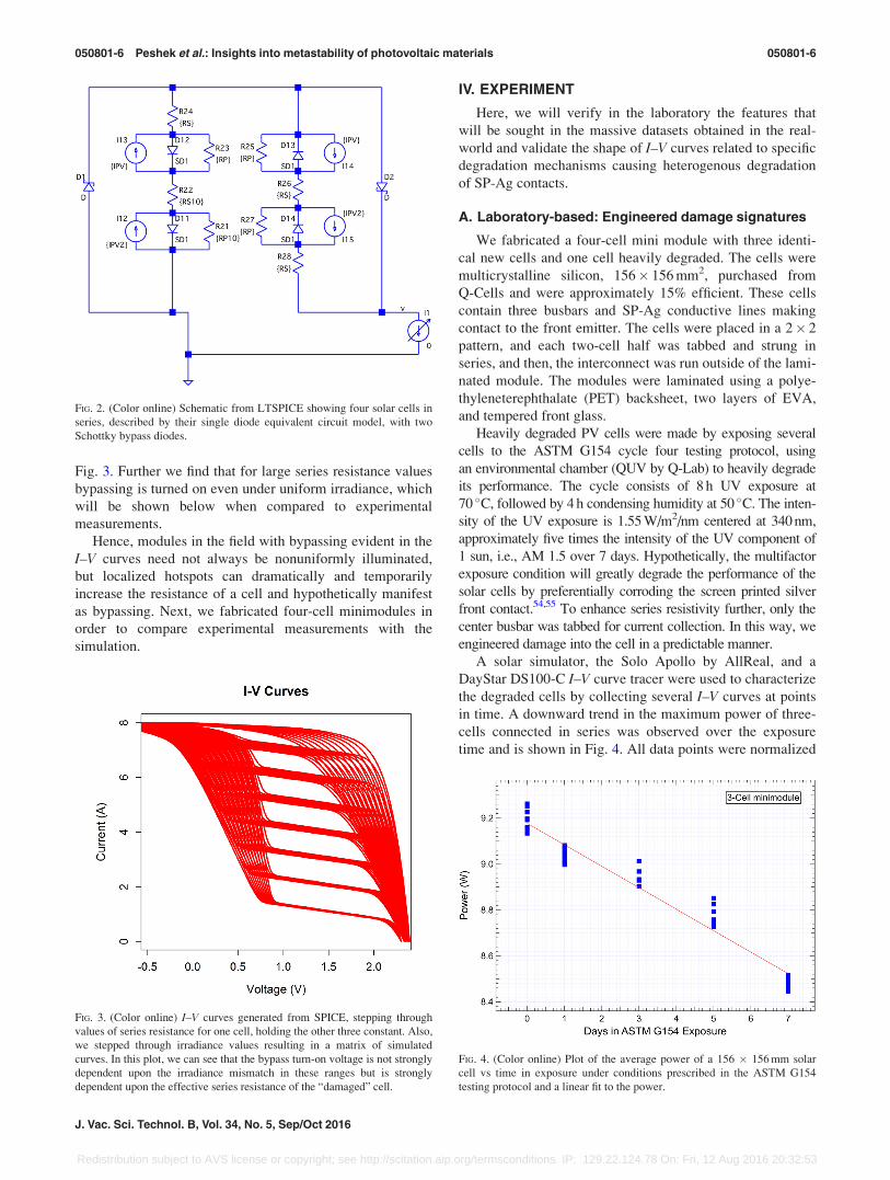
Fig. 3. Further we find that for large series resistance values
bypassing is turned on even under uniform irradiance, which
will be shown below when compared to experimental
measurements.
Hence, modules in the field with bypassing evident in the
I–V curves need not always be nonuniformly illuminated,
but localized hotspots can dramatically and temporarily
increase the resistance of a cell and hypothetically manifest
as bypassing. Next, we fabricated four-cell minimodules in
order to compare experimental measurements with the
simulation.
IV. EXPERIMENT
Here, we will verify in the laboratory the features that
will be sought in the massive datasets obtained in the real-
world and validate the shape of I–V curves related to specific
degradation mechanisms causing heterogenous degradation
of SP-Ag contacts.
A. Laboratory-based: Engineered damage signatures
We fabricated a four-cell mini module with three identi-
cal new cells and one cell heavily degraded. The cells were
multicrystalline silicon, 156� 156 mm2, purchased from
Q-Cells and were approximately 15% efficient. These cells
contain three busbars and SP-Ag conductive lines making
contact to the front emitter. The cells were placed in a 2� 2
pattern, and each two-cell half was tabbed and strung in
series, and then, the interconnect was run outside of the lami-
nated module. The modules were laminated using a polye-
thyleneterephthalate (PET) backsheet, two layers of EVA,
and tempered front glass.
Heavily degraded PV cells were made by exposing several
cells to the ASTM G154 cycle four testing protocol, using
an environmental chamber (QUV by Q-Lab) to heavily degrade
its performance. The cycle consists of 8 h UV exposure at
70 �C, followed by 4 h condensing humidity at 50 �C. The inten-
sity of the UV exposure is 1.55 W/m2/nm centered at 340 nm,
approximately five times the intensity of the UV component of
1 sun, i.e., AM 1.5 over 7 days. Hypothetically, the multifactor
exposure condition will greatly degrade the performance of the
solar cells by preferentially corroding the screen printed silver
front contact.54,55 To enhance series resistivity further, only the
center busbar was tabbed for current collection. In this way, we
engineered damage into the cell in a predictable manner.
A solar simulator, the Solo Apollo by AllReal, and a
DayStar DS100-C I–V curve tracer were used to characterize
the degraded cells by collecting several I–V curves at points
in time. A downward trend in the maximum power of three-
cells connected in series was observed over the exposure
time and is shown in Fig. 4. All data points were normalized
FIG. 2. (Color online) Schematic from LTSPICE showing four solar cells in
series, described by their single diode equivalent circuit model, with two
Schottky bypass diodes.
FIG. 3. (Color online) I–V curves generated from SPICE, stepping through
values of series resistance for one cell, holding the other three constant. Also,
we stepped through irradiance values resulting in a matrix of simulated
curves. In this plot, we can see that the bypass turn-on voltage is not strongly
dependent upon the irradiance mismatch in these ranges but is strongly
dependent upon the effective series resistance of the “damaged” cell.
FIG. 4. (Color online) Plot of the average power of a 156 � 156 mm solar
cell vs time in exposure under conditions prescribed in the ASTM G154
testing protocol and a linear fit to the power.
050801-6 Peshek et al.: Insights into metastability of photovoltaic materials 050801-6
J. Vac. Sci. Technol. B, Vol. 34, No. 5, Sep/Oct 2016
Redistribution subject to AVS license or copyright; see http://scitation.aip.org/termsconditions. IP: 129.22.124.78 On: Fri, 12 Aug 2016 20:32:53

to standard test conditions of 1000 W/m2 and 25 �C. The
thermal coefficient of the maximum power shift is explicitly
provided by the datasheet for the solar cells used and is equal
to 0.43%/K.
B. Outdoor studies
The Solar Durability and Lifetime Extension (SDLE)
Research Center at Case Western Reserve University owns
and operates a unique outdoor test facility, the “SDLE
SunFarm” in Cleveland, OH,56 that provides 14 dual-axis
solar trackers populated with 144 commercial photovoltaic
modules, 122 individual grid-connected photovoltaic power
plants of varying power, and four mirror-augmented PV
(MAPV) modules,57 with controllable nonuniform irradiance
forcing bypass diodes to be forward biased.
The MAPV modules are not grid-connected, but instead
were loaded by a 32 channel DayStar Multitracer, which
provides maximum power point tracking and also scans the
full I–V curve from open circuit voltage (Voc) to Isc at regu-
lar 10 min intervals. Additionally, climatic (weather and
irradiance) metrology is provided by irradiance pyranome-
ters and pyrheliometers (Kipp and Zonen CMP 11 and CHP
1). The weather station (Vaisala WXT520) is capable of
providing measurements58 of air temperature, wind speed,
wind direction, relative humidity, rain intensity, and rain
direction, and these data are collected by a networked
data acquisition system (Campbell Scientific CR1000) on a
minute-by-minute basis.56 T-type thermocouples affixed to
the back of the MAPV modules provide the local tempera-
ture of the module.
Fraunhofer ISE provide us access to their raw outdoor
I–V curve data, tracking data, and supplementary weather
data from three different outdoor test facilities.58–60 These
outdoor test facilities are located at Isla Gran Canaria, Spain
(GC), Mount Zugspitze, Germany (UFS), and Negev Desert,
Isreal (NEG). The sites in GC and UFS have been recording
data since 2010 while the NEG site started recording from
2012. On each of the three sites, I–V curve of two module
samples are measured every 5 min. The maximum power
output of the module is recorded approximately every
minute between sequential I–V measurements.
V. DISCUSSION
A. Engineered damage
We collected irradiance-dependent I–V curves for two
halves of the minimodule with engineered damage, as shown
in Fig. 5. These curves show the disparity in performance
between two cells that are new and two cells where one is
new and one is heavily degraded and highly resistive.
Among the damaged cells, we see that the behavior is not
simply modeled by an increase in the series resistance,
which is evident at voltages near Voc but the slope near short
circuit is also affected. This region of the curve is associated
with the shunt resistance in a diode model system and repre-
sents Ohmic carrier recombination mechanisms. The data
support the interpretation that an increase in the series resis-
tance, which is itself comprised of many factors, is linked to
the shunt resistance in that the resistance cannot support
fully the available current and more photogenerated carriers
are recombining even if the characteristic scattering time is
unchanged in the bulk.
The minimodule fabricated with the damaged cell showed
bypass diode turn-on under uniform irradiance, due to the
resistances of the cells being strongly nonuniform. This
observation demonstrates the potential for real-world mod-
ules to show bypassing even under uniform illumination if a
localized cell or interconnect becomes highly resistive. A
scenario in which this observable may be found is localized
hot spots, where positive thermal feedback occurs because
the photogenerated carriers of a solar cell are thought of as a
current source. Current sources through a resistor can
undergo thermal runaway effects because the power dissipa-
tion is I2R and I is unchanged at the source, but as R increases
the power dissipation increases, causing local heating and a
continual increase in R.
Comparing the measurements of the irradiance-dependent
I–V curves of the minimodule with engineered damage and
SPICE modeling shows similar behavior. The SPICE model
for the minimodules was seeded with measured values from
the individual I–V curves and measurements of the irradi-
ance uniformity in an attempt to closely predict the mini-
module behavior as well as a model for the exact Schottky
bypass diode used, a Hy Electronics 15SQ045. Shunt and
series resistance of the individual cells were extracted by
typical means found in the literature,12 where the shunt resis-
tance was found by fitting a tangent line near I ¼ Isc and
series resistance was approximated by the tangent line near
I¼ 0. These curves are shown in Fig. 6, and although several
similarities arise such as the position and magnitude of the
bypassing even under uniform illumination, and the irradi-
ance in which bypassing disappears, the fill factors of the
simulated and measured curves are very different. In the
FIG. 5. (Color online) Two series of I–V curves as a function of irradiance.
The red series shows the curves acquired from the two cells that were new,
and the blue curves were acquired from the two cells that contained one new
cell and one heavily degraded cell.
050801-7 Peshek et al.: Insights into metastability of photovoltaic materials 050801-7
JVST B - Nanotechnology and Microelectronics: Materials, Processing, Measurement, and Phenomena
Redistribution subject to AVS license or copyright; see http://scitation.aip.org/termsconditions. IP: 129.22.124.78 On: Fri, 12 Aug 2016 20:32:53

simulated curves, the performance of the nonbypassed cells
is quite poor, showing a nearly linear behavior whereas the
experimentally determined curves still demonstrate signifi-
cant curvature.
The comparison of modeled and experimentally deter-
mined I–V curves underscores the potential problems equiva-
lent circuit models, which are potentially insightful, but
incomplete in describing photovoltaic behavior under all
conditions. These conditions can occur under system degra-
dation as well as the nonuniform irradiance that is often
observed relying solely on diode modeling, particularly since
diode models for a complete Si cell gives results that are
inconsistent with experimental data. Hence, we shift to
learnings that can be gained from examining real-world
behavior and subsequent data-driven modeling of anomalous
I–V behavior.
B. Massive analytics of I–V curves
Massive datasets of I–V curves are too burdensome to
analyze one at a time and therefore require taking a statisti-
cal approach with a validated data analytics pipeline.4
These large datasets comprise many climatic variables and
module performance variables, which allow for the demon-
stration of more subtle behaviors that can arise from tran-
sient or permanent changes in the PV modules and can
guide the developments of new models that are more inclu-
sive of heterogeneous behaviors.
The analysis of massive temporal datasets is benefited by
machine learning practices that are implemented in the data
analytics pipeline, which can then be applied to the entire
dataset.
Over 1.5� 106 I–V curves over 500 days have been
acquired on an average interval of 10 min on the SDLE
SunFarm. This massive dataset of I–V curves comprise many
climatic variables and module performance variables, which
allow for the demonstration of more subtle behaviors that
can arise from transient or permanent changes in the PV
modules, and can guide the developments of new models
that are more inclusive of heterogeneous behaviors.
An automatic machine learning pipeline is needed to ade-
quately extract key features from each of the 1.5� 106 I–Vcurves.4 The features of interest in the data include Isc, Voc,
the number of change-points, and the I–V curve slopes, m,
at short circuit and at each change-point. The selection
of features was guided initially by the SPICE development
and extended with empirical evidence. The I–V curves
are grouped into appropriate subpopulations and modeled
accordingly after the feature values are estimated.
The core of this pipeline is a statistical procedure that
involves two parts: change-point detection and parameter
estimation. The change-point detection procedure identifies
the presence and locations of change points in an otherwise
concave I–V curve, by fitting a first or second degree local
polynomial regression48 over the curve and flagging spikes
in residuals. The sensitivity of the algorithm is tuned on a
representative sample that is investigated and labeled by the
researchers. The parameter estimation procedure estimates
current, voltage, and the I–V curve slopes at short circuit
and at each change-point, by, in this case, fitting a first
degree polynomial regression line41 along each I–V curve
and using the linear components as the estimates (see red
lines in Fig. 7). After feature recognition, we next classify
the results. Here, the classification is straightforward and is
based on the number of bypassed strings of cells. For a 60-
cell module, we have three types of curves: type I curves
show a single Voc with no additional change points, type II
shows Voc and 1 additional change point, and type III shows
Voc and two additional change points.
A pairwise scatter and correlation matrix is a useful
method in multivariate analytics for visualizing the learnings
from these massive data. As an example, Fig. 8, generated
using the language “R,”61 shows several variables including
the currents at the intercept of each change point, I1, I2, and
I3 (note that I1 is equivalent to Isc), Voc, maximum power
FIG. 6. (Color online) Series of I–V curves acquired as a function of irradi-
ance for the minimodule with bypass diodes fabricated by combining the
two halves whose I–V curves are shown in Fig. 5 in blue. A comparison to
simulated I–V curves depicted in red is shown. The simulated curves were
seeded with values extracted from I–V curves of the two halves and the data-
sheet of the bypass diodes used in an attempt to match the experimental sce-
nario closely.
FIG. 7. (Color online) Representative type III I–V curve exhibiting three
change points at voltages of 7.35, 16.05 V, and 34 V.
050801-8 Peshek et al.: Insights into metastability of photovoltaic materials 050801-8
J. Vac. Sci. Technol. B, Vol. 34, No. 5, Sep/Oct 2016
Redistribution subject to AVS license or copyright; see http://scitation.aip.org/termsconditions. IP: 129.22.124.78 On: Fri, 12 Aug 2016 20:32:53

point irradiance, and temperature in a pairwise scatter and
correlation matrix. Variables and their histograms are shown
along the matrix diagonal. Below the diagonal shows the
pairwise scatter plots of the variables, and the corresponding
pairwise linear correlation coefficient is shown above the
diagonal. For example, the scatter plot of irradiance versus
Isc is found in the first column, sixth row, and the corre-
sponding linear correlation coefficient of Isc versus irradi-
ance is 0.77, found in the first row, sixth column. This
module was augmented with a mirror to apply nonuniform
irradiance so as to engineer stress into the system as well as
ensure bypass diode turn-on. These data were subset to day-
time measurements only and resulted in approximately 6000
I–V curves over 1 year.
Figure 9 is a bar plot of a small subset of I–V curve data
showing the relative populations of classified I–V curves.
The data set shown was selected from eight days (June 09,
2012 to June 16, 2012) of I–V curves data from the “UFS”
site. On each day, there were 288 measured I–V curves
(5 min time interval, 24 h a day). An I–V curve with less
than ten measurement points will be classified as
“few.points.” Thus I–V curves with a short circuit current
measured less than 1.1 A are classified as “small.amps.”
Figure 9 shows that, on each day, within 288 I–V meas-
urements, a large percentage are classified as either few.-
points or small.amps because I–V measurements were made
continuously day and night during times of little or no mod-
ule illumination. The vast majority of the rest of the I–Vcurves are type I, yet there are type II I–V curves on each
day. This finding supports the idea that many modules will
undergo types II and III behavior in typical installations, at
least in a transient manner and those data can be harvested to
FIG. 8. (Color online) Pairwise scatter and correlation matrix of several variables including the currents at the intercept of each change point, I1, I2, and I3(note that I1 is equivalent to Isc), Voc, maximum power point irradiance, and temperature. Variables and their histograms are shown along the matrix diagonal.
Below the diagonal shows the pairwise scatter plots of the variables, and the corresponding pairwise linear correlation coefficient is shown above the diagonal.
For example, the scatter plot of irradiance vs Isc is found in the first column, sixth row, and the corresponding linear correlation coefficient of Isc vs irradiance
is 0.77, found in the first row, sixth column.
FIG. 9. (Color online) Bar plot of a small subset of I–V curve data showing the relative populations of classified I–V curves. The data set shown was selected
from eight days (June 9, 2012 to June 16, 2012) of I–V curves data from the UFS site. On each day, there were 288 measured I–V curves (5 min time interval,
24 h a day).
050801-9 Peshek et al.: Insights into metastability of photovoltaic materials 050801-9
JVST B - Nanotechnology and Microelectronics: Materials, Processing, Measurement, and Phenomena
Redistribution subject to AVS license or copyright; see http://scitation.aip.org/termsconditions. IP: 129.22.124.78 On: Fri, 12 Aug 2016 20:32:53

gain insights into the performance heterogeneity. Further,
mining these data for the transient behavior of bypass turn-
on as a function of climate may potentially indicate the prev-
alence of performance heterogeneity with climatic stressors.
Therefore, for analysis tracking, the periodicity, or lack
thereof, and the irradiance are critical measures of the
response function of the modules to determine heterogeneity
and discern whether or not the bypassing is externally or
internally caused. This work is ongoing and beyond the
scope of this manuscript. Here, we focus mainly on the
potential for massive data analytics to provide scientific
insights into the mesoscopic solar cell performance.
VI. CONCLUSIONS
Big data analytics is becoming a commonplace term
today, and one that is being invoked in materials science.
We have demonstrated the feasibility and novelty of study-
ing massive I–V datasets spanning many years and including
thousands of curves per year per module using machine
learning techniques. These techniques were validated among
a small set of data and are then useful to devise data analyt-
ics pipelines that enable the analysis and modeling to effi-
ciently be applied to large datasets. I–V curves that are
collected from research facilities in the real-world show
behaviors that are not modeled by simplistic equivalent cir-
cuit models and analytical solving techniques, but these
behaviors and their time dynamics are crucial to understand-
ing heterogeneous degradation. The I–V curves form a link-
age to the laboratory where hypothetical degradation
scenarios can be verified and a more conventional materials
characterization process can be undertaken to identify and
understand the behavior and dynamics of mechanisms.
These linkages then allow for a nonbiased approach to meso-
scale science applied rigorously to the vast scale of real-
world photovoltaic deployment. Our future efforts in this
area will involve classification and examination of the anom-
alous I–V curves collected from outdoor sites, and further
modeling the system heterogeneity as a time-series metric
and comparison to the simulation-aided, laboratory-based
confirmatory experiments.
ACKNOWLEDGMENTS
This work was supported under DOE-EERE SunShot
Award No. DE-EE-0007140. The authors are grateful to the
Department of Energy, Office of Energy Efficiency and
Renewable Energy for their support. The authors are also
grateful to Amy Weaver and Andrew Loach for
contributions to a cover art image associated with this
article.
1J. Hemminger, G. Crabtree, and J. Sarrao, “From quanta to the continuum:
opportunities for mesoscale science,” Technical Report 1183982, U.S.
Department of Energy Basic Energy Sciences Advisory Committee,
September 2012.2G. W. Crabtree and J. L. Sarrao, MRS Bull. 37, 1079 (2012).3J. C. Hemminger, G. Crabtree, and A. Molezemoff, “Science for Energy
Technology: Strengthening the link between basic research and industry,”
US Department of Energy, Office of Science report, Washington, DC,
2010, pp. 1-216, available at http://science.energy.gov/~/media/bes/pdf/
reports/files/setf_rpt_print.pdf (accessed 8 August 2016).4R. H. French et al., Curr. Opin. Solid State Mater. Sci. 19, 212 (2015).5M. Kontges, S. Kurtz, C. Packard, U. Jahn, K. Berger, K. Kato, T. Friesen,
H. Liu, and M. Van Isehegam, “IEA-PVPS {Task 13}: Review of failures
of PV modules,” Technical Report IEA-PVPS T13-01:2014, May 2014.6W. De Soto, S. A. Klein, and W. A. Beckman, Sol. Energy 80, 78 (2006).7A. Hovinen, Phys. Scr. T54, 175 (1994).8Z. Salam, K. Ishaque, and H. Taheri, “An improved two-diode photovol-
taic (PV) model for PV system,” in 2010 Joint International Conferenceon Power Electronics, Drives and Energy Systems (PEDES) 2010 PowerIndia (2010), pp. 1–5.
9M. Taherbaneh, G. Farahani, and K. Rahmani, “Evaluation the accuracy
of one-diode and two-diode models for a solar panel based open-air cli-
mate measurements,” in Solar Cells-Silicon Wafer-Based Technologies(InTech, Craotia, 2011), pp. 512–515.
10A. Jain and A. Kapoor, Sol. Energy Mater. Sol. Cells 81, 269 (2004).11M. Bashahu and P. Nkundabakura, Sol. Energy 81, 856 (2007).12K. Bouzidi, M. Chegaar, and A. Bouhemadou, Sol. Energy Mater. Solar
Cells 91, 1647 (2007).13E. Cuce, P. Mert Cuce, and T. Bali, Appl. Energy 111, 374 (2013).14C. Hansen, “Estimation of parameters for single diode models using mea-
sured IV curves,” in 39th IEEE Photovoltaic Specialists Conference,
Tampa, FL (2013).15F. Khan, S. N. Singh, and M. Husain, Sol. Energy Mater. Sol. Cells 94,
1473 (2010).16T. J. McMahon, T. S. Basso, and S. R. Rummel, “Cell shunt resistance
and photovoltaic module performance,” in Conference Record of theTwenty Fifth IEEE Photovoltaic Specialists Conference (1996), pp.
1291–1294.17Priyanka, M. Lal, and S. N. Singh, Sol. Energy Mater. Sol. Cells 91, 137
(2007).18E. M. G. Rodrigues, R. Mel�ıcio, V. M. F. Mendes, and J. P. S. Catal~ao,
“Simulation of a solar cell considering single-diode equivalent circuit
model,” in International Conference On Renewable Energies And PowerQuality, Spain (2011), pp. 13–15.
19D. Sera and R. Teodorescu, “Robust series resistance estimation for diag-
nostics of photovoltaic modules,” in 35th Annual Conference of IEEEIndustrial Electronics, 2009. IECON’09 (2009), pp. 800–805.
20D. Sera, “Series resistance monitoring for photovoltaic modules in the
vicinity of MPP,” in 25th European Photovoltaic Solar EnergyConference and Exhibition (2010), pp. 4506–4510.
21A. Jain, S. Sharma, and A. Kapoor, Sol. Energy Mater. Sol. Cells 90, 25
(2006).22F. Ghani, M. Duke, and J. Carson, Sol. Energy 91, 422 (2013).23G. Petrone, G. Spagnuolo, and M. Vitelli, Sol. Energy Mater. Sol. Cells
91, 1652 (2007).24T. J. Peshek, S. Mathews, Y. Hu, and R. H. French, “Mirror augmented
photovoltaics and time series analytics of the I-V curve parameters,” in
40th IEEE Photovoltaic Specialist Conference (PVSC) (2014), pp.
2027–2031.25S. Sellner, J. Sutterlueti, S. Ransome, L. Schreier, and N. Allet,
“Understanding PV module performance: Further validation of the novel
loss factors model and its extension to AC arrays,” in 27th EuropeanPhotovoltaic Solar Energy Conference and Exhibition (2012), pp.
3199–3204.26S. Sellner, J. Sutterluti, L. Schreier, and S. Ransome, “Advanced PV mod-
ule performance characterization and validation using the novel Loss
Factors Model,” in 2012 38th IEEE Photovoltaic Specialists Conference(PVSC), June (2012), pp. 002938–002943.
27J. S. Stein, J. Sutterlueti, S. Ransome, C. W. Hansen, and B. H. King,
“Outdoor PV performance evaluation of three different models: single-
diode, SAPM and loss factor model,” in EU PVSEC Proccedings (2013),
pp. 2865–2871.28I. B. Cooper, K. Tate, J. S. Renshaw, A. F. Carroll, K. R. Mikeska, R. C.
Reedy, and A. Rohatgi, IEEE J. Photovoltaics 4, 134 (2014).29Y. M. Chiang, L. A. Silverman, R. H. French, and R. M. Cannon, J. Am.
Ceram. Soc. 77, 1143 (1994).30S. B. Rane, P. K. Khanna, T. Seth, G. J. Phatak, D. P. Amalnerkar, and B.
K. Das, Mater. Chem. Phys. 82, 237 (2003).31E. Kossen, B. Heurtault, and A. F. Stassen, “Comparison of two step print-
ing methods for front side metallization,” in Proceedings of the 25th
050801-10 Peshek et al.: Insights into metastability of photovoltaic materials 050801-10
J. Vac. Sci. Technol. B, Vol. 34, No. 5, Sep/Oct 2016
Redistribution subject to AVS license or copyright; see http://scitation.aip.org/termsconditions. IP: 129.22.124.78 On: Fri, 12 Aug 2016 20:32:53

European Photovoltaic Solar Energy Conference, Valencia, Spain (2010),
pp. 2099–2100.32H. Hannebauer, T. Dullweber, T. Falcon, and R. Brendel, Energy Procedia
38, 725 (2013).33H. Hannebauer, T. Dullweber, T. Falcon, X. Chen, and R. Brendel, Energy
Procedia 43, 66 (2013).34Z. G. Li, L. Liang, A. S. Ionkin, B. M. Fish, M. E. Lewittes, L. K. Cheng,
and K. R. Mikeska, J. Appl. Phys. 110, 074304 (2011).35M. Z. Burrows, A. Meisel, D. Balakrishnan, A. Tran, D. Inns, E. Kim, A.
F. Carroll, and K. R. Mikeska, 39th IEEE Photovoltaic SpecialistsConference (PVSC) (IEEE, 2013), pp. 2171–2175.
36D. Pysch, A. Mette, A. Filipovic, and S. W. Glunz, Prog. Photovoltaics 17,
101 (2009).37A. Mette, D. Pysch, G. Emanuel, D. Erath, R. Preu, and S. W. Glunz,
Prog. Photovoltaics 15, 493 (2007).38F. Gao, Z. Li, M. E. Lewittes, K. R. Mikeska, P. D. VerNooy, and L. Kin
Cheng, J. Electrochem. Soc. 158, B1300 (2011).39L. S. Bruckman, N. R. Wheeler, J. Ma, E. Wang, C. K. Wang, I. Chou, J.
Sun, and R. H. French, IEEE Access 1, 384 (2013).40International Energy Agency, Performance and Reliability of Photovoltaic
Systems: Task 13 (International Energy Agency, Technical Report IEA-
PVPS T13-01:2014, March 2014).41G. James, D. Witten, T. Hastie, and R. Tibshirani, An Introduction to
Statistical Learning: With Applications in R, Springer Texts in Statistics,
1st ed. (Springer, New York, 2013), corr. 5th printing 2015 edition.42T. Hastie, R. Tibshirani, and J. Friedman, The Elements of Statistical
Learning, Springer Series in Statistics (Springer, New York, 2009).43D. M. Riley and G. K. Venayagamoorthy, “Comparison of a recurrent neu-
ral network PV system model with a traditional component-based PV sys-
tem model,” in 37th IEEE Photovoltaic Specialists Conference (PVSC)(IEEE, 2011), pp. 002426–002431.
44D. Riley and J. Johnson, “Photovoltaic prognostics and heath management
using learning algorithms,” in 38th IEEE Photovoltaic SpecialistsConference (PVSC) (2012), pp. 001535–001539.
45A. Dali, A. Bouharchouche, and S. Diaf, “Parameter identification of
photovoltaic cell/module using genetic algorithm (GA) and particle
swarm optimization (PSO),” in 3rd International Conference onControl, Engineering and Information Technology (CEIT) (IEEE, 2015),
pp. 1–6.
46K. Ishaque, Z. Salam, H. Taheri, and A. Shamsudin, “Parameter extrac-
tion of photovoltaic cell using differential evolution method,” in 2011IEEE Applied Power Electronics Colloquium (IAPEC), April (2011),
pp. 10–15.47O. Hachana, K. E. Hemsas, G. M. Tina, and C. Ventura, J. Renewable
Sustainable Energy 5, 053122 (2013).48G. James, D. Witten, T. Hastie, and R. Tibshirani, “Moving beyond
linearity-local regression,” in An Introduction to Statistical Learning: WithApplications in R, Springer Texts in Statistics, 1st ed. (Springer, New
York, 2013), Chap. 7.6, pp. 280–282; corr. 5th printing 2015 edition.49T. Hastie and R. Tibshirani, J. R. Stat. Soc., Ser. B 55, 757 (1993).50B. D. Ripley and R Core Team, R: Local Polynomial Regression Fitting
(R Foundation for Statistical Computing, Vienna, Austria, 2016).51L. Castaner and S. Silvestre, Modeling Photovoltaic Systems Using PSpice
(Counterpoint, Washington, D.C., 2002).52A. Zekry and A. Y. Al-Mazroo, IEEE Trans. Electron Devices 43, 691
(1996).53S. Eidelloth, F. Haase, and R. Brendel, IEEE J. Photovoltaics 2, 572 (2012).54M. Koehl, M. Heck, and S. Wiesmeier, Sol. Energy Mater. Sol. Cells 99,
282 (2012).55H. Shalaby, Sol. Cells 14, 51 (1985).56Y. Hu, M. A. Hosain, T. Jain, Y. R. Gunapati, L. Elkin, G. Q. Zhang, and R.
H. French, “Global SunFarm data acquisition network, energy CRADLE,
and time series analysis,” in 2013 IEEE Energytech, May (2013), pp. 1–5.57W. Lin, T. J. Peshek, L. S. Bruckman, M. A. Schuetz, and R. H. French,
IEEE J. Photovoltaics 5, 917 (2015).58M. K€ohl, “From climate data to accelerated test conditions,” Fraunhofer
Institute for Solar Energy Systems, Freiburg, Germany, paper presented at
the PVMRW, Golden (CO, USA), 2011, http://www1.eere.energy.gov/
solar/pdfs/pvmrw2011_05_plen_kohl.pdf.59J. Herrmann, T. Lorenz, K. Slamova, E. Klimm, M. Koehl, and K.-A.
Weiss, “Desert applications of PV modules,” in 40th IEEE PhotovoltaicSpecialist Conference (PVSC) (IEEE, 2014), pp. 2043–2046.
60M. Koehl, M. Heck, S. Wiesmeier, and J. Wirth, Sol. Energy Mater. Sol.
Cells 95, 1638 (2011).61R Core Team, R: A Language and Environment for Statistical Computing
(R Foundation for Statistical Computing, Vienna, Austria, 2015), available
at https://cran.r-project.org/doc/manuals/r-release/fullrefman.pdf (accessed
6 August 2016).
050801-11 Peshek et al.: Insights into metastability of photovoltaic materials 050801-11
JVST B - Nanotechnology and Microelectronics: Materials, Processing, Measurement, and Phenomena
Redistribution subject to AVS license or copyright; see http://scitation.aip.org/termsconditions. IP: 129.22.124.78 On: Fri, 12 Aug 2016 20:32:53


![RSC Advances - [engineering.case.edu]engineering.case.edu/centers/sdle/sites/engineering.case.edu... · Received 13th January 2012, Accepted 21st October ... specificity in sorting](https://img.pdfslide.us/doc/110x75/5ab645a47f8b9ab47e8daa46/rsc-advances-13th-january-2012-accepted-21st-october-specificity-in-sorting.jpg)