Embed Size (px)
Citation preview
Safe Trajectory Planning of Autonomous Vehicles
by
Tom Schouwenaars
Burgerlijk Elektrotechnisch IngenieurKatholieke Universiteit Leuven (2001)
Submitted to the Department of Aeronautics and Astronauticsin partial fulfillment of the requirements for the degree of
Doctor of Philosophy
at the
MASSACHUSETTS INSTITUTE OF TECHNOLOGY
February 2006
c© Massachusetts Institute of Technology 2006. All rights reserved.
Author . . . . . . . . . . . . . . . . . . . . . . . . . . . . . . . . . . . . . . . . . . . . . . . . . . . . . . . . . . . . . . . . . . . . . . . . . . . .Department of Aeronautics and Astronautics
November 18, 2005
Certified by. . . . . . . . . . . . . . . . . . . . . . . . . . . . . . . . . . . . . . . . . . . . . . . . . . . . . . . . . . . . . . . . . . . . . . . .Eric Feron
Associate Professor of Aeronautics and AstronauticsThesis Supervisor
Certified by. . . . . . . . . . . . . . . . . . . . . . . . . . . . . . . . . . . . . . . . . . . . . . . . . . . . . . . . . . . . . . . . . . . . . . . .Jonathan P. How
Associate Professor of Aeronautics and AstronauticsThesis Supervisor
Certified by. . . . . . . . . . . . . . . . . . . . . . . . . . . . . . . . . . . . . . . . . . . . . . . . . . . . . . . . . . . . . . . . . . . . . . . .Munther Dahleh
Professor of Electrical Engineering and Computer ScienceThesis Supervisor
Accepted by . . . . . . . . . . . . . . . . . . . . . . . . . . . . . . . . . . . . . . . . . . . . . . . . . . . . . . . . . . . . . . . . . . . . . . .Jaime Peraire
Professor of Aeronautics and AstronauticsChairman, Department Committee on Graduate Students

2
Safe Trajectory Planning of Autonomous Vehiclesby
Tom Schouwenaars
Submitted to the Department of Aeronautics and Astronauticson November 18, 2005, in partial fulfillment of the
requirements for the degree ofDoctor of Philosophy
Abstract
This thesis presents a novel framework for safe online trajectory planning of unmannedvehicles through partially unknown environments. The basic planning problem is formulatedas a receding horizon optimization problem using mixed-integer linear programming (MILP)to incorporate kino-dynamic, obstacle avoidance and collision avoidance constraints. Agilevehicle dynamics are captured through a hybrid control architecture that combines severallinear time-invariant modes with a discrete set of agile maneuvers. The latter are representedby affine transformations in the state space and can be described using a limited numberof parameters. We specialize the approach to the case of a small-scale helicopter flyingthrough an urban environment.
Next, we introduce the concept of terminal feasible invariant sets in which a vehicle canremain for an indefinite period of time without colliding with obstacles or other vehicles.These sets are formulated as affine constraints on the last state of the planning horizon andas such are computed online. They guarantee feasibility of the receding horizon optimizationat future time steps by providing an a priori known backup plan that is dynamically feasibleand obstacle-free. Vehicle safety is ensured by maintaining a feasible return trajectory ateach receding horizon iteration. The feasibility and safety constraints are essential whenthe vehicle is maneuvering through environments that are only partially characterized andfurther explored online. Such a scenario was tested on an unmanned Boeing aircraft usingscalable loiter circles as feasible invariant sets.
The terminal feasible invariant set concept forms the basis for the construction of aprovably safe distributed planning algorithm for multiple vehicles. Each vehicle then onlycomputes its own trajectory while accounting for the latest plans and invariant sets of theother vehicles in its vicinity, i.e., of those whose reachable sets intersect with that of theplanning vehicle. Conflicts are solved in real-time in a sequential fashion that maintainsfeasibility for all vehicles over all future receding horizon iterations. The algorithm is appliedto the free flight paradigm in air traffic control and to a multi-helicopter relay network aimedat maintaining wireless line of sight communication in a cluttered environment.
Thesis Supervisor: Eric FeronTitle: Associate Professor of Aeronautics and Astronautics
Thesis Supervisor: Jonathan P. HowTitle: Associate Professor of Aeronautics and Astronautics
Thesis Supervisor: Munther DahlehTitle: Professor of Electrical Engineering and Computer Science
3

4
Acknowledgments
This dissertation is the result of a fruitful collaboration with my advisor Prof. Eric Feronand co-advisor Prof. Jonathan How. I am extremely grateful for their guidance over thelast four years and for creating an environment in which I enjoyed significant academic andorganizational freedom. I am indebted to Eric’s unconditional support, both on a moraland financial level (including sponsoring for many trips), and thank him for the continuedtrust he placed in me. His energy, openness, and out of the box ideas have never stoppedimpressing me. He made the lab a fun place to work. Jon was in a way my processand quality control manager. I thank him for the many detailed discussions on researchproblems and patient revisions of (usually last-minute) paper manuscripts. His dedicationto research, publishing and teaching are exemplary. Finally, I would like to thank my thirdcommittee member, Prof. Munther Dahleh, for his valuable input during the last semesters.
The long days (and nights) in LIDS would not have been the same without the socialcontacts with my colleague students, many of whom became close friends. I have vividmemories of the daily conversations and sharing of frustrations (in Flemish) with Jan DeMot, the lunches and cookie follow-ups with Masha Ishutkina, the espresso breaks andlaughs with Julius Kusuma, the Boeing visits and related 3 AM food trips to La Verde’swith Mario Valenti, the humor and cycling expertise of Chris Dever, the discussions onintellectual property with Gregory Mark, the introduction to Iranian culture by MardavijRoozbehani, the research and conference trips with Bernard Mettler, the late night exchangeof politics opinions with Selcuk Bayraktar, and the discussions on academia vs. industrywith Vishwesh Kulkarni. Over the years, the friendly and cooperative atmosphere in thelab was further completed by Animesh Chakravarthy, Han-Lim Choi, Emily Craparo, DavidDugail, Vladislav Gavrilets, Sommer Gentry, John Harper, Farmey Joseph, Georgios Kot-salis, Jerome Le Ny, Rodin Lyasoff, Ioannis Martinos, Nuno Martins, Mitra Osqui, NavidSabagghi, Keith Santarelli, Danielle Taraf, Olivier Toupet, Glenn Tournier, and Ji HyunYang, all of whom I frequently interacted with in the office or corridor. The administrativestaff made all processes run smoothly. A special word of thanks goes to Lauren Clark,Angela Copyak, Kathryn Fisher, Lisa Gaumond, Doris Inslee, and Margaret Yoon, and toMarie Stuppard for providing flexibility with departmental deadlines on several occasions.
During the course of my studies, I had the opportunity to work with various non-MIT organizations, which gave me insight into how engineering is practised outside of theacademic world. I would like to thank Dr. Mark Tischler for hosting me at Nasa Ames andBoeing Phantom Works in St. Louis for the cooperation on the Software Enabled ControlProgram. Last summer, I worked intensely with Dr. Andrew Stubbs and Dr. James Paduanofrom Nascent Technology Corporation. I am also grateful to Prof. Emile Boulpaep, theBelgian American Educational Foundation and the Francqui Foundation for providing thefinancial support to start my studies at MIT.
Despite the many hours spent in the lab and working on problem sets at home, therewas a life beside these duties, for which I could count on a large group of friends. The MITEuropean Club gave me the chance to actively participate in the foreign student scene in theBoston area. The rich social interactions added to the already incredible mix of cultures atMIT and resulted in many friendships for life. I am also grateful to Michael Garcia-Webb,my roommate during the last years, for the many conversations in the evenings and forcoping with my shifted night schedule. I also have great memories of the weekend partieswith our Sidney-Pacific friends, at least of those I did not have to bail out because of someupcoming deadline. On my short trips home, family and friends were always available for
5

having a good time, and Klaartje Genbrugge’s regular emails and the moral support of mysoulmate Carolina Diaz-Quijano have kept me sane during the last months.
Finally, I am grateful to my parents for supporting me in my choices and making mebelieve in myself. To them I dedicate this thesis.
6
Contents
1 Introduction 17
1.1 Autonomous Trajectory Planning . . . . . . . . . . . . . . . . . . . . . . . . 17
1.1.1 Unmanned Vehicles . . . . . . . . . . . . . . . . . . . . . . . . . . . 17
1.1.2 Trajectory Planning Problem . . . . . . . . . . . . . . . . . . . . . . 18
1.1.3 Guidance System Hierarchy . . . . . . . . . . . . . . . . . . . . . . . 19
1.2 Literature Overview . . . . . . . . . . . . . . . . . . . . . . . . . . . . . . . 20
1.2.1 Non-MPC Trajectory Planning Methods . . . . . . . . . . . . . . . . 20
1.2.2 MPC-based Trajectory Planning . . . . . . . . . . . . . . . . . . . . 22
1.3 Statement of Contributions . . . . . . . . . . . . . . . . . . . . . . . . . . . 23
1.4 Thesis Outline . . . . . . . . . . . . . . . . . . . . . . . . . . . . . . . . . . 25
2 Receding Horizon Trajectory Planning 27
2.1 Introduction . . . . . . . . . . . . . . . . . . . . . . . . . . . . . . . . . . . . 27
2.2 Problem Formulation . . . . . . . . . . . . . . . . . . . . . . . . . . . . . . . 28
2.2.1 Problem Setup . . . . . . . . . . . . . . . . . . . . . . . . . . . . . . 28
2.2.2 Receding Horizon Planning . . . . . . . . . . . . . . . . . . . . . . . 29
2.2.3 Optimization Problem . . . . . . . . . . . . . . . . . . . . . . . . . . 30
2.3 MILP Formulation . . . . . . . . . . . . . . . . . . . . . . . . . . . . . . . . 31
2.3.1 Mixed Integer Linear Programming . . . . . . . . . . . . . . . . . . . 32
2.3.2 Vehicle Dynamics . . . . . . . . . . . . . . . . . . . . . . . . . . . . . 32
2.3.3 Obstacle Avoidance . . . . . . . . . . . . . . . . . . . . . . . . . . . 34
2.3.4 Collision Avoidance . . . . . . . . . . . . . . . . . . . . . . . . . . . 37
2.4 Example Scenarios . . . . . . . . . . . . . . . . . . . . . . . . . . . . . . . . 37
2.4.1 Example 1: UAV in 2D . . . . . . . . . . . . . . . . . . . . . . . . . 37
2.4.2 Example 2: Multiple UAVs in 2D . . . . . . . . . . . . . . . . . . . . 38
2.4.3 Example 3: Helicopter in 3D . . . . . . . . . . . . . . . . . . . . . . 39
2.5 Conclusion . . . . . . . . . . . . . . . . . . . . . . . . . . . . . . . . . . . . 40
3 Hybrid Model for Agile Vehicles 43
3.1 Introduction . . . . . . . . . . . . . . . . . . . . . . . . . . . . . . . . . . . . 43
3.2 Hybrid Control Architecture for Guidance . . . . . . . . . . . . . . . . . . . 44
3.2.1 Automatic Control of Agile Vehicles . . . . . . . . . . . . . . . . . . 44
3.2.2 Velocity Control System . . . . . . . . . . . . . . . . . . . . . . . . . 45
3.2.3 Maneuver Scheduler . . . . . . . . . . . . . . . . . . . . . . . . . . . 47
3.2.4 LTI-Maneuver Automaton . . . . . . . . . . . . . . . . . . . . . . . . 48
3.3 Trajectory Optimization with the LTI-MA . . . . . . . . . . . . . . . . . . . 48
3.3.1 Sequential decision process . . . . . . . . . . . . . . . . . . . . . . . 48
7
3.3.2 Trajectory Optimization Using MILP . . . . . . . . . . . . . . . . . 49
3.3.3 Planning Strategies . . . . . . . . . . . . . . . . . . . . . . . . . . . . 51
3.4 Small-Scale Helicopter Example . . . . . . . . . . . . . . . . . . . . . . . . . 53
3.4.1 Helicopter LTI Modes . . . . . . . . . . . . . . . . . . . . . . . . . . 53
3.4.2 Helicopter Maneuvers . . . . . . . . . . . . . . . . . . . . . . . . . . 58
3.4.3 Obstacle Avoidance . . . . . . . . . . . . . . . . . . . . . . . . . . . 60
3.4.4 Receding Horizon Formulation . . . . . . . . . . . . . . . . . . . . . 62
3.5 Results . . . . . . . . . . . . . . . . . . . . . . . . . . . . . . . . . . . . . . . 63
3.5.1 Helicopter and Problem Parameters . . . . . . . . . . . . . . . . . . 63
3.5.2 Scenarios . . . . . . . . . . . . . . . . . . . . . . . . . . . . . . . . . 64
3.5.3 Hardware in the Loop Experiments . . . . . . . . . . . . . . . . . . . 68
3.6 Practical Considerations . . . . . . . . . . . . . . . . . . . . . . . . . . . . . 68
3.7 Conclusion . . . . . . . . . . . . . . . . . . . . . . . . . . . . . . . . . . . . 69
4 Trajectory Planning with Feasibility and Safety Guarantees 71
4.1 Introduction . . . . . . . . . . . . . . . . . . . . . . . . . . . . . . . . . . . . 71
4.2 Unsafe Scenarios . . . . . . . . . . . . . . . . . . . . . . . . . . . . . . . . . 72
4.3 Feasibility Constraints . . . . . . . . . . . . . . . . . . . . . . . . . . . . . . 73
4.3.1 Feasible Invariant Sets . . . . . . . . . . . . . . . . . . . . . . . . . . 73
4.3.2 Feasible Receding Horizon Planning Problem . . . . . . . . . . . . . 75
4.4 Feasible Invariant Sets as Affine Transformations . . . . . . . . . . . . . . . 76
4.4.1 Terminal Feasible Invariant Set Modeling . . . . . . . . . . . . . . . 76
4.4.2 Sampling Points Requirements . . . . . . . . . . . . . . . . . . . . . 77
4.4.3 MILP Formulation . . . . . . . . . . . . . . . . . . . . . . . . . . . . 79
4.4.4 Examples . . . . . . . . . . . . . . . . . . . . . . . . . . . . . . . . . 80
4.5 Safety Constraints . . . . . . . . . . . . . . . . . . . . . . . . . . . . . . . . 82
4.5.1 Safety Definitions . . . . . . . . . . . . . . . . . . . . . . . . . . . . . 82
4.5.2 Safe Feasible Receding Horizon Planning Problem . . . . . . . . . . 85
4.5.3 Backtrack Pattern . . . . . . . . . . . . . . . . . . . . . . . . . . . . 88
4.5.4 Safe Receding Horizon Planning without Feasibility Guarantees . . . 89
4.6 Conclusion . . . . . . . . . . . . . . . . . . . . . . . . . . . . . . . . . . . . 91
5 Safe Distributed Trajectory Planning for Multiple Vehicles 93
5.1 Introduction . . . . . . . . . . . . . . . . . . . . . . . . . . . . . . . . . . . . 93
5.2 Problem Formulation . . . . . . . . . . . . . . . . . . . . . . . . . . . . . . . 95
5.2.1 Receding Horizon Planning . . . . . . . . . . . . . . . . . . . . . . . 95
5.2.2 Safety Principle . . . . . . . . . . . . . . . . . . . . . . . . . . . . . . 96
5.2.3 Conflict Description . . . . . . . . . . . . . . . . . . . . . . . . . . . 96
5.2.4 Communication Requirements . . . . . . . . . . . . . . . . . . . . . . 97
5.3 Safe Trajectory Planning Algorithm . . . . . . . . . . . . . . . . . . . . . . 100
5.3.1 Algorithm . . . . . . . . . . . . . . . . . . . . . . . . . . . . . . . . . 100
5.3.2 Remarks . . . . . . . . . . . . . . . . . . . . . . . . . . . . . . . . . . 101
5.4 Implementation Using MILP . . . . . . . . . . . . . . . . . . . . . . . . . . 102
5.4.1 Aircraft Model . . . . . . . . . . . . . . . . . . . . . . . . . . . . . . 103
5.4.2 Loiter Circles . . . . . . . . . . . . . . . . . . . . . . . . . . . . . . . 104
5.4.3 Avoidance Constraints . . . . . . . . . . . . . . . . . . . . . . . . . . 104
5.4.4 Cost Function . . . . . . . . . . . . . . . . . . . . . . . . . . . . . . . 106
5.5 Results . . . . . . . . . . . . . . . . . . . . . . . . . . . . . . . . . . . . . . . 106
8

5.6 Conclusion . . . . . . . . . . . . . . . . . . . . . . . . . . . . . . . . . . . . 108
6 Multi-Vehicle Path Planning for Non-Line of Sight Communication 1116.1 Introduction . . . . . . . . . . . . . . . . . . . . . . . . . . . . . . . . . . . . 1116.2 Problem Formulation . . . . . . . . . . . . . . . . . . . . . . . . . . . . . . . 113
6.2.1 Problem Setup . . . . . . . . . . . . . . . . . . . . . . . . . . . . . . 1136.2.2 Centralized Receding Horizon Planning . . . . . . . . . . . . . . . . 1146.2.3 Connectivity Constraints . . . . . . . . . . . . . . . . . . . . . . . . 115
6.3 Implementation . . . . . . . . . . . . . . . . . . . . . . . . . . . . . . . . . . 1166.3.1 Helicopter Test-Bed . . . . . . . . . . . . . . . . . . . . . . . . . . . 1166.3.2 Mission Scenario . . . . . . . . . . . . . . . . . . . . . . . . . . . . . 1176.3.3 Trajectory Planning Software . . . . . . . . . . . . . . . . . . . . . . 118
6.4 Results . . . . . . . . . . . . . . . . . . . . . . . . . . . . . . . . . . . . . . . 1196.4.1 Planning Parameters . . . . . . . . . . . . . . . . . . . . . . . . . . . 1196.4.2 Simulation and Flight Test Results . . . . . . . . . . . . . . . . . . . 120
6.5 Distributed Planning Strategy . . . . . . . . . . . . . . . . . . . . . . . . . . 1236.5.1 Distributed Cooperative Algorithm . . . . . . . . . . . . . . . . . . . 1236.5.2 Results . . . . . . . . . . . . . . . . . . . . . . . . . . . . . . . . . . 125
6.6 Conclusion . . . . . . . . . . . . . . . . . . . . . . . . . . . . . . . . . . . . 126
7 Implementation of MILP-based UAV Guidance for Human/UAV Team 1297.1 Introduction . . . . . . . . . . . . . . . . . . . . . . . . . . . . . . . . . . . . 1297.2 Experiment and Technology Overview . . . . . . . . . . . . . . . . . . . . . 130
7.2.1 Mission Scenario . . . . . . . . . . . . . . . . . . . . . . . . . . . . . 1307.2.2 Technology Development . . . . . . . . . . . . . . . . . . . . . . . . 133
7.3 Natural Language Parsing and Interfacing . . . . . . . . . . . . . . . . . . . 1337.4 Task Scheduling and Communications Interfacing . . . . . . . . . . . . . . . 1357.5 MILP-based Trajectory Generation Module . . . . . . . . . . . . . . . . . . 136
7.5.1 MILP Formulation . . . . . . . . . . . . . . . . . . . . . . . . . . . . 1367.5.2 Implementation . . . . . . . . . . . . . . . . . . . . . . . . . . . . . . 139
7.6 Simulation and Flight Test Results . . . . . . . . . . . . . . . . . . . . . . . 1417.6.1 Simulation Results . . . . . . . . . . . . . . . . . . . . . . . . . . . . 1427.6.2 Flight-Test Results . . . . . . . . . . . . . . . . . . . . . . . . . . . . 144
7.7 Conclusion . . . . . . . . . . . . . . . . . . . . . . . . . . . . . . . . . . . . 148
8 Conclusion 1498.1 Summary . . . . . . . . . . . . . . . . . . . . . . . . . . . . . . . . . . . . . 1498.2 Future Work . . . . . . . . . . . . . . . . . . . . . . . . . . . . . . . . . . . 150
9

10
List of Figures
1-1 Boeing’s Unmanned Combat Aerial Vehicle (UCAV) . . . . . . . . . . . . . 18
1-2 Hierarchical decomposition of a guidance system into three decision and con-trol layers . . . . . . . . . . . . . . . . . . . . . . . . . . . . . . . . . . . . . 19
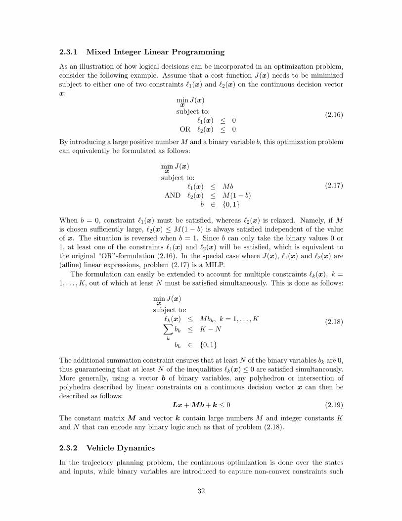
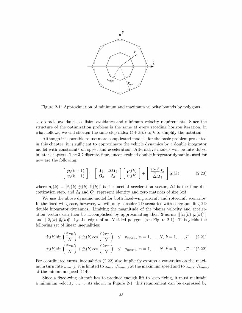
2-1 Approximation of minimum and maximum velocity bounds by polygons. . . 33
2-2 Approximation of an arbitrary 2D obstacle by its convex hull and with convexpolygons filling up the concavities. The vehicle is allowed to be inside thered areas, but must stay outside the grey area. . . . . . . . . . . . . . . . . 35
2-3 Example 1: The aircraft is initially in the origin, flying east at 4 m/s, andhas to maneuver to position (70, 57) m. The goal is reached after 28 s. . . . 38
2-4 Example 2: The aircraft are initially positioned along a circle and need tofly to the opposite side. A conflict in the middle is avoided thanks to thecollision avoidance constraints. . . . . . . . . . . . . . . . . . . . . . . . . . 39
2-5 Example 3: The helicopter is initially hovering in position (30,−60, 8) m, andhas to maneuver to hover in position (125, 60, 10) m. The goal is reached after14 s. . . . . . . . . . . . . . . . . . . . . . . . . . . . . . . . . . . . . . . . . 40
2-6 Two-dimensional projection of Example 3 . . . . . . . . . . . . . . . . . . . 41
3-1 Hybrid control architecture: the helicopter can be controlled through a ve-locity control system, or through a maneuver scheduler that allows the im-plementation of agile maneuvers taken from a library. . . . . . . . . . . . . 46
3-2 Abstract representation of the control architecture. The linear controllersallow continuous motion, the maneuvers are discrete transitions. . . . . . . 46
3-3 Graph representation of the LTI-maneuver automaton. The vehicle is eitherin an LTI mode, or executing a finite duration maneuver. . . . . . . . . . . 48
3-4 Example of operating regions of the velocity control mode, shown in functionof the body axis forward (u) and lateral velocity (v). . . . . . . . . . . . . . 54
3-5 Two circle approximation of the elliptic constraint on forward and lateralacceleration. . . . . . . . . . . . . . . . . . . . . . . . . . . . . . . . . . . . . 56
3-6 Polygonal approximation of minimum and maximum velocity bounds delim-iting the various LTI-modes. . . . . . . . . . . . . . . . . . . . . . . . . . . . 57
3-7 Helicopter trajectories for sample maneuvers. . . . . . . . . . . . . . . . . . 59
3-8 Change in helicopter position and orientation resulting from a maneuver(shown in dashed line), as observed from the body-fixed frame . . . . . . . 60
3-9 Scenario 1: The helicopter is initially in (0, 0) flying at 12 m/s and needsto reverse direction towards (−100, 0) as quickly as possible. It decides toexecute the split-S. . . . . . . . . . . . . . . . . . . . . . . . . . . . . . . . . 65
11
3-10 Scenario 2: The helicopter is initially in (0, 0) flying at 6 m/s and needs toreverse direction towards (−100, 0) as quickly as possible. It decides to makea U-turn. . . . . . . . . . . . . . . . . . . . . . . . . . . . . . . . . . . . . . 65
3-11 Scenario 3: The helicopter is initially in (0, 0) flying at 12 m/s and needsto reverse direction towards (−100, 0) as quickly as possible. To avoid theobstacle in the middle, it decides to change heading before executing thesplit-S. . . . . . . . . . . . . . . . . . . . . . . . . . . . . . . . . . . . . . . . 66
3-12 Scenario 4: The helicopter is initially in (0, 0) flying at 6 m/s and needsto reverse direction towards (−100, 0) as quickly as possible. To avoid theobstacle in the middle, it decides to make wider a U-turn. . . . . . . . . . . 66
3-13 Scenario 5: The helicopter is initially in (0, 0) flying at 12 m/s and needsto reverse direction towards (−100, 0) as quickly as possible. Because of thenarrower corridor, the vehicle first turns northeast before executing the split-S. 67
3-14 Scenario 6: The helicopter is initially in (0, 0) flying at 12 m/s and needs toreverse direction towards (−100, 0) as quickly as possible. The only feasibleoption is to slow down and make a turn on the spot. . . . . . . . . . . . . . 67
3-15 Hardware in the loop experiments. The helicopter is flying between twoobstacles, initially heading east at 10 m/s. Figure (a) shows the helicopterreversing direction by slowing down till hover and turning on the spot. InFigure (b), it performs a hammerhead. The different actions depend on thewidth of the corridor. . . . . . . . . . . . . . . . . . . . . . . . . . . . . . . 68
4-1 The aircraft is initially in the origin, flying east at 4 m/s, and has to ma-neuver to position (70, 57) m. After 17 s, the MILP becomes infeasible,corresponding to the aircraft colliding with the obstacles. . . . . . . . . . . 73
4-2 The aircraft are initially positioned along a circle and need to fly to theopposite side. Near the origin, the MILP becomes infeasible: the aircrafthave approached each other too closely and an intersection of their avoidancezones cannot be avoided. . . . . . . . . . . . . . . . . . . . . . . . . . . . . . 74
4-3 Safe trajectory ending in either a right or left turning loiter circle. . . . . . 77
4-4 Situation where undersampling of the loiter circle leads to a safety viola-tion. Although the obstacle avoidance constraints for the sample points aresatisfied, the circle intersects the obstacle. . . . . . . . . . . . . . . . . . . . 78
4-5 Situation where the loiter circle cuts the corner of an obstacle. This situationcan be avoided by enlarging the obstacles with a safety boundary dsafe. . . . 78
4-6 Receding horizon trajectory with loiter constraints. Because of the loiterconstraints, the UAV avoids the concavity and chooses an alternative routeto reach the goal. . . . . . . . . . . . . . . . . . . . . . . . . . . . . . . . . . 80
4-7 Sequence of intermediate receding horizon trajectories ending in loiter circles. 80
4-8 Receding horizon trajectory with loiter constraints. Although the UAV entersthe concavity, it does not crash and the trajectory ends in a loiter. . . . . . 81
4-9 Sequence of intermediate receding horizon trajectories for a wider concavity.Although the UAV enters the concavity, it does not crash and the trajectoryends in a loiter. . . . . . . . . . . . . . . . . . . . . . . . . . . . . . . . . . . 81
4-10 Feasible receding horizon trajectory with loiter constraints. . . . . . . . . . 82
4-11 Sequence of intermediate receding horizon trajectories with loiter constraintsconsisting of 24 sample points. . . . . . . . . . . . . . . . . . . . . . . . . . 82
12
4-12 Scenario in which the terminal feasible invariant set constraints cannot pre-vent the UAV from getting trapped inside a concavity. Although feasibilityis maintained, actual vehicle safety is not. . . . . . . . . . . . . . . . . . . . 83
4-13 Intermediate receding horizon trajectories ending in loiter circles for the sce-nario in which the UAV gets trapped inside a concavity. . . . . . . . . . . . 84
4-14 Safe receding horizon trajectory of T time steps ending in a terminal feasibleinvariant set S(t + T |t) and with backtrack pattern B(t + T |t) to the returntrajectory T (t). . . . . . . . . . . . . . . . . . . . . . . . . . . . . . . . . . . 85
4-15 Intermediate receding horizon trajectories with backtrack pattern. The ve-hicle now avoids entering and getting trapped in the concavity because theloiter circle with additional backtrack pattern do not fit inside of it. . . . . 88
4-16 Intermediate receding horizon trajectories with backtrack patterns that arenot geometrically constrained and can join the return trajectory in any onestate of a given subset. . . . . . . . . . . . . . . . . . . . . . . . . . . . . . . 89
4-17 Safe receding horizon trajectory without feasibility guarantees. The red tri-angles indicate positions where the problem became infeasible (but safetywas maintained). . . . . . . . . . . . . . . . . . . . . . . . . . . . . . . . . . 90
4-18 Intermediate receding horizon trajectories with safety patterns that do notcontain a terminal invariant set. . . . . . . . . . . . . . . . . . . . . . . . . . 90
5-1 Simulation results for distributed conflict resolution of 2 and 4 aircraft for 30time steps of 5 s each. . . . . . . . . . . . . . . . . . . . . . . . . . . . . . . 107
5-2 Computation times at each iteration for the 2 aircraft scenario of Figure 5-1a.108
5-3 Computation times at each iteration for the 4 aircraft scenario of Figure 5-1b.108
5-4 Safe trajectories and corresponding loiter boxes for the 4 aircraft scenarioduring the first 9 time steps (corresponding to 45 s). . . . . . . . . . . . . . 109
5-5 Safe trajectories of 8 aircraft during 40 time steps of 5 s each. . . . . . . . . 109
5-6 Safe trajectories of 10 aircraft during 65 time steps of 5 s each. . . . . . . . 110
6-1 MIT’s autonomous X-Cell helicopter, equipped with avionics box. . . . . . . 116
6-2 Satellite image of the test region. The rectangle represents the take-off areaand ground station, the circle is the target location. Source: Google Earth . 118
6-3 Nominal trajectories of the Burlington scenario computed in Matlab usingreceding horizon planning. The circles represent the mission helicopter, thetriangles show the relay vehicle. The obstacles in the center are buildings;the large no-fly zone at the Western and Southern edge represents forests(enlarged with a safety boundary). . . . . . . . . . . . . . . . . . . . . . . . 121
6-4 Hardware-in-the-loop simulations of the trajectories computed online in real-time. The circles represent the mission helicopter; the triangles show the relayvehicle. . . . . . . . . . . . . . . . . . . . . . . . . . . . . . . . . . . . . . . 121
6-5 Actual flight test data of the trajectories computed online in real-time. Thecircles represent the mission helicopter; the triangles show the relay vehicle. 122
6-6 Simulation result for distributed Burlington scenario with extra obstacle andsecond relay vehicle. . . . . . . . . . . . . . . . . . . . . . . . . . . . . . . . 126
6-7 Simulation result for distributed scenario in which the mission helicoptermust fly over the building (MIT’s Simmons Hall) and the relay has to gainaltitude. . . . . . . . . . . . . . . . . . . . . . . . . . . . . . . . . . . . . . . 127
13
7-1 SEC Capstone Demonstration test vehicles . . . . . . . . . . . . . . . . . . 1317-2 Overview of the MIT flight experiment . . . . . . . . . . . . . . . . . . . . . 1327-3 Block diagram of the MIT SEC Capstone Demonstration system. “FCS”
stands for Flight Control System, “GIB” for Guy-in-Back (i.e., the rear-seatoperator). . . . . . . . . . . . . . . . . . . . . . . . . . . . . . . . . . . . . . 134
7-4 Sample scenario map for the MIT SEC Capstone Demonstration. The flightarea is approximately 40 mi long along the northern boundary. . . . . . . . 141
7-5 SEC demonstration Simulation-In-the-Loop (SIL) laboratory setup . . . . . 1427-6 SIL Test 1 - Initialization of the SEC demonstration: the UAV (in light)
enters a loiter pattern. . . . . . . . . . . . . . . . . . . . . . . . . . . . . . 1437-7 SIL Test 2 - Pop-up obstacle test: the UAV safely avoids both pop-up threats.1447-8 SIL Test 3 - Simulated flight with two consecutive search missions. . . . . . 1457-9 Flight experiment system level diagram . . . . . . . . . . . . . . . . . . . . 1457-10 SEC Flight-Test: UAV/T-33 (in light) with simulated F-15 (in dark) . . . . 1467-11 SEC Flight-Test: UAV/T-33 (in light) and actual F-15 (in dark) providing
natural language commands. . . . . . . . . . . . . . . . . . . . . . . . . . . 147
14
List of Tables
3.1 Description of sample maneuvers that could be implemented on a rotorcraft-type vehicle. . . . . . . . . . . . . . . . . . . . . . . . . . . . . . . . . . . . . 58
3.2 Parameters of LTI modes . . . . . . . . . . . . . . . . . . . . . . . . . . . . 633.3 Parameters of pre-programmed maneuvers . . . . . . . . . . . . . . . . . . . 64
6.1 Parameters used in the MILP trajectory optimization . . . . . . . . . . . . 119
15

16
Chapter 1
Introduction
1.1 Autonomous Trajectory Planning
1.1.1 Unmanned Vehicles
In recent years, autonomous vehicles have become increasingly important assets in variouscivilian and military operations. A wide variety of robotic vehicles is currently in useor being developed, ranging from unmanned fixed-wing aircraft, helicopters, blimps andhovercraft to ground and planetary rovers, earth-orbiting spacecraft and deep-space probes.Although the level of autonomy differs among the types of vehicles and the missions theyare used for, many such systems require no or minor human control from a base or groundstation. The primary reason for deploying autonomous vehicles is often a reduction in costor elimination of human risk associated with a particular mission: unmanned systems donot require operator safety and life support systems, and can therefore be made smallerand cheaper than their manned counterparts. Furthermore, autonomous vehicles enableoperations in remote or harsh environments and often possess the capability to operatecontinuously or complete missions that are of longer duration than ones manned systemsare capable of.
In this dissertation, we are mainly interested in autonomous rotorcraft and fixed-wingaircraft, or so-called unmanned aerial vehicles (UAVs). One such vehicle, Boeing’s UCAV,is pictured in Figure 1-1. Although their development has primarily been motivated bymilitary needs [101], such as unmanned combat missions and reconnaissance and surveillanceoperations, there are many civilian applications of interest. They include search and rescueoperations, surveillance of natural disaster sites such as (possibly remote) areas hit byan earthquake or flood, and inspection of environments that are typically inaccessible tohumans, such as active volcanic craters or sites where high radioactive radiation is present.Other applications are urban surveillance, traffic monitoring, weather observation, freightservices, and the creation of spectacular camera shots in the movie and advertising industry.Some of these might require cooperative behavior between multiple vehicles. For example,in an urban environment where wireless line of sight communication with a ground station isobstructed by buildings, a team of multiple vehicles can act as an autonomous relay network.Finally, autonomy technologies developed for UAVs can contribute to the improvement orautomation of the commercial air traffic management system.
17
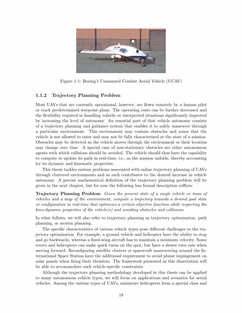
Figure 1-1: Boeing’s Unmanned Combat Aerial Vehicle (UCAV)
1.1.2 Trajectory Planning Problem
Most UAVs that are currently operational, however, are flown remotely by a human pilotor track predetermined waypoint plans. The operating costs can be further decreased andthe flexibility required in handling volatile or unexpected situations significantly improvedby increasing the level of autonomy. An essential part of that vehicle autonomy consistsof a trajectory planning and guidance system that enables it to safely maneuver througha particular environment. This environment may contain obstacles and zones that thevehicle is not allowed to enter and may not be fully characterized at the start of a mission.Obstacles may be detected as the vehicle moves through the environment or their locationmay change over time. A special case of non-stationary obstacles are other autonomousagents with which collisions should be avoided. The vehicle should thus have the capabilityto compute or update its path in real-time, i.e., as the mission unfolds, thereby accountingfor its dynamic and kinematic properties.
This thesis tackles various problems associated with online trajectory planning of UAVsthrough cluttered environments and as such contributes to the desired increase in vehicleautonomy. A precise mathematical definition of the trajectory planning problem will begiven in the next chapter, but for now the following less formal description suffices:
Trajectory Planning Problem: Given the present state of a single vehicle or team ofvehicles and a map of the environment, compute a trajectory towards a desired goal stateor configuration in real-time that optimizes a certain objective function while respecting thekino-dynamic properties of the vehicle(s) and avoiding obstacles and collisions.
In what follows, we will also refer to trajectory planning as trajectory optimization, pathplanning, or motion planning.
The specific characteristics of various vehicle types pose different challenges to the tra-jectory optimization. For example, a ground vehicle and helicopter have the ability to stopand go backwards, whereas a fixed-wing aircraft has to maintain a minimum velocity. Somerovers and helicopters can make quick turns on the spot, but have a slower turn rate whenmoving forward. Reconfiguring satellite clusters or spacecraft maneuvering around the In-ternational Space Station have the additional requirement to avoid plume impingement onsolar panels when firing their thrusters. The framework presented in this dissertation willbe able to accommodate such vehicle-specific constraints.
Although the trajectory planning methodology developed in this thesis can be appliedto many autonomous vehicle types, we will focus on applications and scenarios for aerialvehicles. Among the various types of UAVs, miniature helicopters form a special class and
18
are particularly interesting for operations in cluttered environments. Besides their abilityto hover at a fixed location, fly at low speeds, and turn on the spot, they can exhibit veryagile behavior enabling quick obstacle avoidance in changing environments and fast napof-the-earth flight. Taking advantage of these capabilities in an automated fashion is oneof the problems tackled in this thesis.
1.1.3 Guidance System Hierarchy
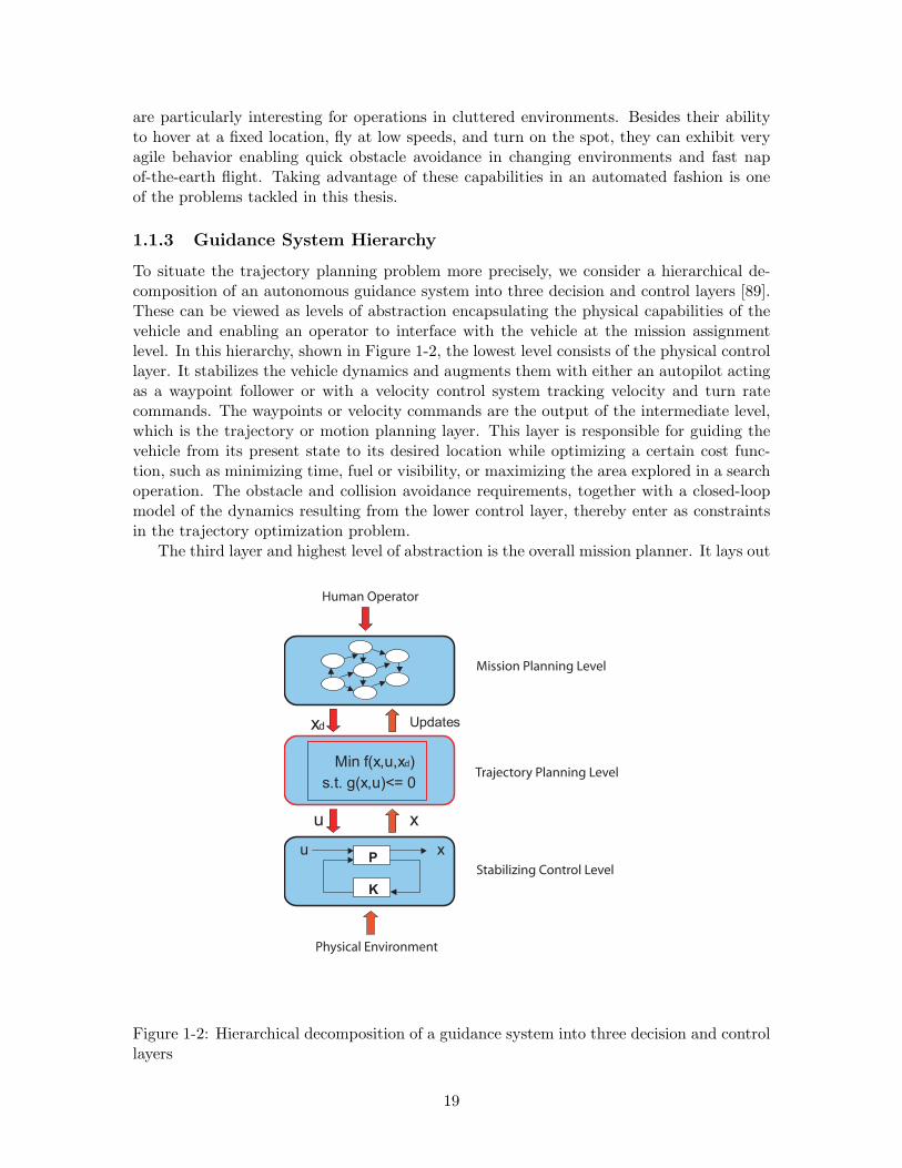
To situate the trajectory planning problem more precisely, we consider a hierarchical de-composition of an autonomous guidance system into three decision and control layers [89].These can be viewed as levels of abstraction encapsulating the physical capabilities of thevehicle and enabling an operator to interface with the vehicle at the mission assignmentlevel. In this hierarchy, shown in Figure 1-2, the lowest level consists of the physical controllayer. It stabilizes the vehicle dynamics and augments them with either an autopilot actingas a waypoint follower or with a velocity control system tracking velocity and turn ratecommands. The waypoints or velocity commands are the output of the intermediate level,which is the trajectory or motion planning layer. This layer is responsible for guiding thevehicle from its present state to its desired location while optimizing a certain cost func-tion, such as minimizing time, fuel or visibility, or maximizing the area explored in a searchoperation. The obstacle and collision avoidance requirements, together with a closed-loopmodel of the dynamics resulting from the lower control layer, thereby enter as constraintsin the trajectory optimization problem.
The third layer and highest level of abstraction is the overall mission planner. It lays out
P
KK
Min f(x,u,xd)
s.t. g(x,u)<= 0
u x
u x
xd Updates
Mission Planning Level
Stabilizing Control Level
Human Operator
Physical Environment
Trajectory Planning Level
Figure 1-2: Hierarchical decomposition of a guidance system into three decision and controllayers
19
a sequence of task waypoints that accomplish the particular mission and act as subsequentgoal locations at the intermediate trajectory planning level. Examples of such higher levelmissions are the UAV applications given above. In case multiple vehicles are involved, thislayer is also responsible for the individual task assignment [130, 6, 113, 78]. To remain com-putationally tractable, simplified descriptions of the environment and the vehicle’s physicalcapabilities resulting from the lower levels are typically used when generating the missionplan [27, 28, 99]. However, the various models used in this hierarchy should be consistent,i.e. the behaviors commanded by the higher decision layers should be executable by thelower layers [104, 105].
We can now say more specifically that this dissertation develops the intermediate trajec-tory design level assuming that both the higher mission planning and lower physical controllayers are in place.
1.2 Literature Overview
Motion planning has been an important research topic in the field of robotics and arti-ficial intelligence for several decades. The earliest methods tackled trajectory planningfor holonomic systems operating in an environment without obstacles and were based onoptimal control [1, 24] and nonlinear programming techniques [16]. A survey of such nu-merical methods can be found in [20]. In this dissertation, however, we are interestedin tackling the motion planning problem in the presence of obstacles and other vehicles.Many methods have been developed, and it is not our ambition to give a thorough sur-vey of all of these. Instead, we will broadly distinguish between recent techniques basedon model predictive control (MPC) and earlier methods, many of which were developedin the artificial intelligence community and some of which yielded fundamental complexityresults [110, 49, 111, 26].
1.2.1 Non-MPC Trajectory Planning Methods
The classic monograph by Latombe [72] presents many of the basic concepts and complexityresults related to robot motion planning. A more recent book by LaValle [74] also coversthe latest methods in the field. Other survey works include the papers by Schwartz andSharir [132, 133], Hwang and Narendra [54], and Latombe [73]. An overview of specificmethods for spacecraft formation flying and reconfiguration can be found in the work ofSharf et al. [123, 124]. In addition, Frazzoli [35] gives a classification of the various kino-dynamic motion planning problems in free or obstacle environments in terms of nonlinearcontrol problems.
Among the basic concepts in motion planning is the notion of the configuration space,in which the size of the vehicle is added to the obstacles [80, 52]. As such, the vehicleitself is reduced to a point mass. In case the orientation of the vehicle is of importance tobeing able to pass an obstacle, e.g., in the so-called piano mover’s problem [110, 131, 77],an extra dimension is introduced in which the size of the obstacle changes with the vehicle’sorientation. The configuration space is generally used in the various algorithmic motionplanning methods.
The first methods developed in the artificial intelligence community were based on dy-namic programming algorithms [17, 138] for graph searching formulations of the motionplanning problem. Among those are cell decomposition or surface covering methods inwhich the configuration space is partitioned into a finite number of regions and the motion
20
planning problem is reduced to finding a sequence of neighboring cells [80, 81]. Other graphsearching methods are so-called roadmap techniques where a network of feasible paths isconstructed among which a sequence of connecting paths between the initial and final con-figuration is selected. Visibility graphs [82] and Voronoi diagrams [30] are examples of suchroadmap constructions.
Most of these early methods, however, use simplified kinematic models of the vehiclesor robots, which may lead to conservative results. For example, the full dynamic capa-bilities may not be exploited, or a safety margin may have to be included that accountsfor uncertainties in the actual motion when the kinematic reference trajectory is trackedby a lower level control law. Although they were initially used with kinematic models aswell [65, 151, 3], artificial potential field methods do allow to account for the dynamics ofthe vehicle [92, 11, 119]. In these methods, obstacles and other vehicles are modeled asrepelling forces in a potential field by being embedded as peaks in a potential function.Using numerical optimization techniques, the gradient of the latter is then used to steer thevehicle towards the global minimum of the function corresponding to the desired state.
Although potential function methods can produce smooth, dynamically feasible trajec-tories, they have several disadvantages. A first problem is that the vehicle might get trappedin a local minimum. A second issue arises from the fact that obstacles are not modeledas hard constraints. In addition, obstacles typically have to be modeled as continuous anddifferentiable functions, leading to an imprecise description of the obstacle’s shape and di-mensions. Especially when the vehicle has to maneuver through tight environments, thesesoft constraints cannot provide hard avoidance guarantees.
Alternative methods that produce dynamically feasible trajectories with hard avoidanceguarantees are based on so-called rapidly-exploring random trees (RRTs) [75, 60]. Thesetrees consist of feasible trajectories that are built online by extending branches towardsrandomly generated target states. The RRT methods form a subset of the larger class ofstochastic optimization [88] and randomized motion planning algorithms [61, 2], the first ofwhich were probabilistic roadmap (PRM) planners [62, 63, 51, 21]. PRM algorithms combinean offline construction of a roadmap with a randomized online selection of an appropriatepath from the roadmap. Unlike RRT methods, however, these algorithms cannot be appliedin rapidly changing environments due to the offline construction of the roadmap.
Randomized algorithms were introduced to circumvent the intrinsic exponential com-plexity of the motion planning problem. Reif [110] indeed showed that the problem of findinga path for a robot consisting of several polyhedral parts through an environment with poly-hedral obstacles is PSPACE-hard. Schwartz and Sharir [131] constructed an algorithm fornon-polyhedral obstacles whose time complexity is twice exponential in the dimension nof the configuration space and polynomial in the number and degree of polynomial con-straints describing the obstacles. Canny [26] found a more efficient algorithm that is singleexponential in n. Fundamental complexity results for problems involving multiple robotswere derived by Hopcroft et al. [49] and Reif and Sharir [111]. A topological approach toestablish the complexity of nonholonomic motion planning was carried out by Jean [58].
To further reduce the complexity associated with including the detailed vehicle dynamicsin the problem formulation, methods using motion primitives were introduced. Marigo andBicchi [87] used control quanta, whereas Frazzoli [35, 36] proposed the concept of a maneuverautomaton. The latter consists of a discrete set of trim conditions and transitions betweenthese trims that are called maneuvers. Using dynamic programming, a value function iscomputed offline that gives the optimal time between a particular vehicle state and a desiredstate, whereby the trajectories consist of a sequence of trims and maneuvers. The value
21
function is used in an online control policy and obstacle avoidance is obtained using rapidly-exploring random trees. In this dissertation, we will generalize this automaton framework toan approach that includes continuous trim modes and permits to include obstacle avoidancedirectly in the optimization.
Other recent methods that account for precise nonlinear dynamics are based on iterativemethods using splines [95, 79] or nonlinear programming [53, 108]. To be applicable in real-time, however, they must be combined with a receding horizon planning strategy as isdiscussed next.
1.2.2 MPC-based Trajectory Planning
The trajectory planning methodology and concepts that are developed in this thesis belongto the class of model predictive control-based motion planning. Similarly to the randomizedand motion primitive approaches described above, these algorithms aim at reducing thecomplexity of the planning problem and do so by repeatedly solving online a constrainedoptimization problem over a finite planning horizon. At each iteration, a segment of thetotal path is computed using on a dynamic model of the vehicle that predicts its futurebehavior. More specifically, a sequence of control inputs and resulting vehicle states isgenerated that meet the kino-dynamic and environment constraints and that optimize someperformance objective. Only a subset of these inputs is actually implemented, however, andthe optimization is repeated as the vehicle maneuvers and new measurements of the vehiclestates and the environment are obtained. As such, this approach is especially useful whenthe environment is explored online.
Model predictive control (MPC) or receding horizon control (RHC) originated in theprocess industry a few decades ago, and has since received wide attention in the broaderfield of control theory and other applications. The benefits of the approach is that it allowsto naturally handle multivariable sytems, can systematically take actuator limitations intoaccount, and allows a system to operate closer to its constraints, therefore often resultingin better performance [85]. The survey papers by Garcia et al. [38], Morari and Li [98],Mayne et al. [91, 90], and Rawlings [109] offer a good introduction to the field.
Because of this flexibility, in recent years, receding horizon control has been introducedto the problem of trajectory planning as well. Initially, most work only tackled problemsin obstacle-free environments [48, 57] or was limited to tracking predetermined trajectoriesaround obstacles [139]. However, Bemporad et al. [11] have used potential functions tomodel obstacles and Dunbar et al. [32] have used splines to produce collision-free trajecto-ries.
In [125, 127] an alternative receding horizon approach based on mixed-integer linearprogramming (MILP) was introduced. MILP is a powerful optimization framework thatallows inclusion of integer variables and discrete logic in a continuous linear optimizationproblem. These variables can be used to model logical constraints such as obstacle andcollision avoidance rules, while the dynamic and kinematic properties of the vehicle areformulated as continuous constraints. An overview of applications and algorithms to solveMILP problems can be found in [33]. It is still an active research topic in the field ofOperations Research [144, 152], and the state of the art in cutting plane methods, branch-and-bound algorithms, integral basis methods, and approximation algorithms is covered inthe recent book by Bertsimas and Weismantel [19].
The main advantage of using MILP for trajectory planning is that it can systemati-cally handle hard obstacle and collision avoidance constraints and allows to include other
22
decision features such as task assignment into the optimization problem. Moreover, thealgorithms are complete, i.e., they give a feasible solution if one exists. Although devel-oped independently in [127], the MILP-based trajectory planning approach is a specialcase of the broader class of control for mixed logical dynamical (MLD) systems, developedby Bemporad and Morari in [12]. They provide a general method for formulating hybridsystem dynamics in a mathematical framework using a combination of real and binaryvariables. Explicit solutions for piecewise linear optimal controllers were later derived viaoff-line multi-parametric MILP [9, 22]. Such controllers divide the space into polyhedralregions in which different linear controllers are optimal. The results for MLD systems ex-tended earlier results for discrete-time linear time-invariant systems that were based onmulti-parametric quadratic [14] and linear programming [10] for finding the optimal MPCcontrollers explicitly.
Unfortunately, although these methods provide an elegant solution to the general prob-lem, they cannot handle the computational complexity of a typical trajectory planningproblem and are not very useful in dynamic environments. Online optimization of a lessgeneral (i.e., smaller) problem for specific initial vehicle states is therefore of more interest.As demonstrated by the results in [116] and [129], thanks to the increase in computer speedand implementation of powerful state of the art algorithms in software packages such asCPLEX [56], MILP has become a feasible option for real-time path planning. Throughoutthis dissertation, we will provide more references to ongoing research and work on relatedtopics and alternative approaches that was done in parallel at MIT and other universities.
1.3 Statement of Contributions
This thesis presents several new concepts for receding horizon trajectory planning of bothsingle and multiple vehicles. The majority of the ideas and algorithms that are introducedcan be considered independent of the underlying optimization method and as such can begenerally used with path planning techniques other than MILP. Furthermore, some of theconcepts fit within the broader field of MPC of hybrid systems. In this dissertation, however,we restrict ourselves to guidance problems and choose to illustrate the theory using MILPas the implementation framework. The contributions of this thesis can then be stated asfollows:
• We introduce a general hybrid dynamic model for trajectory planning of highly agilevehicles. The proposed control architecture combines a velocity control system con-sisting of various continuous linear time-invariant modes with a discrete set of agilemaneuvers. The latter are represented by affine transformations in the state spaceand can be described using a limited number of parameters such as the maneuverduration, displacement, and ingress and egress conditions such as entrance and exitvelocity. The model efficiently captures the agile, nonlinear capabilities of the vehiclein a way that is well-suited for real-time trajectory planning using MILP. Comparedto the maneuver automaton from [35], the required library of LTI modes and agilemaneuvers is much smaller, more precise navigation is possible and obstacle avoid-ance constraints can be directly included in the trajectory optimization. We specializethe approach to a model of a small-scale rotorcraft based on MIT’s aerobatic X-Cellhelicopter.
• We extend the principle of receding horizon trajectory planning by including feasibil-
23
ity and safety guarantees in the problem formulation. We introduce the concept of aterminal feasible invariant set in which the vehicle can safely remain for an indefiniteperiod of time. These sets are expressed as collections of affine transformations of thelast state in the planning horizon and as such are computed online. Constraining thereceding horizon trajectory computed at each iteration to terminate in such an invari-ant set guarantees nominal feasibility of the optimization problem at all future timesteps. Safety is ensured by maintaining an a priori known backtrack trajectory thatis updated at each receding horizon iteration. The feasibility and safety constraintsare essential when maneuvering through environments that are only partially char-acterized and further explored online. Unlike other approaches such as [4, 146] ourformulation does not require intensive off-line computations of fixed invariant sets. Assuch, it allows for more flexible and less conservative solutions for maintaining vehiclesafety through cluttered environments.
• We use the terminal feasible invariant set concept for single vehicles to develop anew and fast algorithm for provably safe distributed trajectory planning for multiplevehicles. All vehicles that are within a certain conflict zone of each other will subse-quently update and broadcast their paths. Each vehicle thereby only plans its owntrajectory using a receding horizon strategy that accounts for the latest plans of allother vehicles in the conflict zone. The algorithm is applied to multiple aircraft wherefuture feasibility of the planning problem is guaranteed by maintaining dynamicallyfeasible trajectories for all aircraft that terminate in non-intersecting loiter patterns.Besides maintaining feasibility, if the problem is too complex to be solved within thetime constraints of a real-time system, our approach also provides a priori safe rescuesolutions for each vehicle. The algorithm is also applicable to maintaining nominalfeasibility of a general distributed planning problem and can be used with any tra-jectory optimization technique that has collision avoidance guarantees. We present aMILP implementation and corresponding collision avoidance constraints.
• A proof-of-concept application is given of MILP-based multi-vehicle receding horizonpath planning with feasibility guarantees. The problem of interest is to maintainwireless communication between a ground station and a vehicle that is performing amission in a cluttered environment. Relay agents are therefore introduced that mustbe positioned throughout the environment in such a way that an indirect line of sightconnection with the ground station is always maintained. We present a centralizedand a distributed receding horizon algorithm that achieves such cooperation in a waythat is more flexible than existing approaches. Feasibility at future time steps isensured by using hover states as terminal feasible invariant sets. Obstacle avoidance,connectivity and collision avoidance constraints are again formulated using MILP. Afirst-time flight-test of multi-vehicle online MILP-based trajectory planning with twohelicopters through a real obstacle environment was performed.
• Successful implementation and flight-test demonstration of single vehicle MILP-basedreceding horizon trajectory planning were done using an autonomous T-33 aircraft. Incooperation with Boeing Phantom Works and as part of DARPA’s Software EnabledControl Program, a mission was flown through a partially unknown environment.Obstacle-free trajectories with feasibility guarantees were computed on-board the ve-hicle in real-time, adapting the flight path to pop-up no-fly zones and changing missiontasks.
24
• Numerous improvements to the basic MILP path planning formulation as introducedin [127, 125] are made. An efficient representation of arbitrarily shaped non-convexobstacles is developed that requires fewer binary variables and inequalities. Severalvehicle models with new kino-dynamic constraints are introduced that capture heli-copter and fixed-wing dynamics more precisely than the basic double integrator model.Alternative cost functions are presented for minimum time trajectories that yield com-parable results but are much faster than exact shortest time formulations and allow forshorter planning horizons. Finally, several simplifications and heuristics are discussedthat reduce the computational requirements in practical implementations.
1.4 Thesis Outline
The dissertation is organized as follows. Chapter 2 formalizes the basic receding horizontrajectory planning problem for single and multiple vehicles. The corresponding MILP for-mulation and various example scenarios for navigation through a cluttered environment aregiven. Chapter 3 then presents a hybrid control architecture for agile vehicles that enablesinclusion of nonlinear maneuvers in the receding horizon optimization problem. Next, Chap-ter 4 extends the basic receding horizon strategy to include feasibility and safety constraints.It introduces the concept of a terminal feasible invariant set that is computed online andshould be reachable from all states along the trajectory. Various simulation scenarios inwhich the feasibility and/or safety constraints prove to be essential are presented. Chap-ter 5 then uses the terminal feasible invariant set principle for a single vehicle to constructa safe distributed planning algorithm for multiple vehicles. A detailed description of thealgorithm along with a formal feasibility proof and simulation results for multiple aircraftare given. In Chapter 6, the concepts of the previous chapters are combined and applied tothe problem of multi-vehicle path planning for maintaining indirect line of sight communi-cation between vehicles in a cluttered environment. Simulation, hardware in the loop andflight-test results of a two-helicopter mission are given. Next, Chapter 7 presents anotherflight-test demonstration involving a piloted F-15 and an autonomous T-33 aircraft guidedby a MILP-based trajectory planner. An overview of the software architecture and naturallanguage interface between the vehicles is given, and details and results of the MILP-basedguidance system are discussed. Chapter 8 then concludes the thesis and outlines some topicsfor future work.
25

26
Chapter 2
Receding Horizon TrajectoryPlanning
This chapter presents the basic trajectory planning problem for single and multiple vehiclesusing a receding horizon planning strategy. A high-level mathematical problem statementis given in the form of an online optimization problem for which a mixed-integer program-ming implementation is worked out in detail. Constraints for general obstacle and collisionavoidance are presented and a cost function is introduced that automatically switches froman approximate to an exact minimum time objective once the goal is within reach. Thegenerality and flexibility of the MILP-based trajectory planning approach are illustratedthrough several single and multi-vehicle scenarios.
2.1 Introduction
As discussed in Chapter 1, over the last decade, both civilian and military institutionshave expressed increased interest in the use of fully autonomous aircraft and helicopters orso-called unmanned aerial vehicles (UAVs) [101]. Such systems need no, or minor, humancontrol from a ground station, thereby reducing operating costs and enabling missions inharsh or remote environments. A significant part of the vehicle autonomy consists of itspath planning capabilities: the problem is to guide the vehicle through an obstacle fieldwhile accounting for its dynamic and kinematic properties.
In many applications, a detailed map of the environment is not available ahead oftime, and obstacles are detected while the mission is carried out. In this chapter, weconsider scenarios where the environment is only known within a certain detection radiusaround the vehicle. We assume that within that region, the environment is static and fullycharacterized. The knowledge of the environment could either be gathered through thedetection capabilities of the vehicle itself, or result from cooperation with another, moresophisticated agent [94, 149].
Since the environment is explored online, a trajectory from a start to a destination lo-cation typically needs to be computed gradually over time, i.e., while the mission unfolds.This calls for a receding horizon strategy, in which a new segment of the total path iscomputed at each time step by solving a constrained optimization problem over a limitedhorizon. In [125, 127] a receding horizon approach based on mixed-integer linear program-ming was introduced that provides hard obstacle and collision avoidance guarantees, andallows inclusion of other non-convex state and input constraints. The basic MILP receding
27
horizon formulation presented in [127] was extended to account for local minima in [7]. Inthe latter, a cost-to-go function was introduced based on a graph representation of the wholeenvironment between start and end point that guaranteed stability in the sense of reachingthe goal. The approach has been further extended to account for turn rate constraintsin [68] and for planning through three dimensional environments in [69].
In this chapter, however, we assume that the environment is not fully characterizedbefore the mission. As such, a visibility graph as in [7] can only be constructed locally usinga line of sight approximation of the distance to the goal beyond the detection radius. Such aheuristic will be used in Chapter 7. Here we will instead return to the basic formulation andfocus on the dynamic, kinematic, obstacle avoidance and collision avoidance constraints. Anextended MILP formulation for avoidance of arbitrarily shaped non-convex obstacles anda new switching cost function for guiding a vehicle to its goal state in a fast way areintroduced.
2.2 Problem Formulation
2.2.1 Problem Setup
This section presents the basic trajectory planning problem for a team of vehicles thatwas outlined in Chapter 1 more formally. Let the various agents be denoted by an indexi = 1, . . . , V . For optimization purposes, the dynamics of each vehicle are characterized bydiscrete-time, linear state space models as follows:
xi(t + 1) = Aixi(t) + Biui(t), i = 1, . . . , V (2.1)
where xi(t) ∈ RNx is the state vector and ui(t) ∈ R
Nu is the input vector at the tth timestep. The state vector xi(t) is typically made up of the position and velocity in a 3D inertialcoordinate frame (east, north, altitude), respectively denoted by pi(t) ≡ [xi(t) yi(t) zi(t)]
′ ∈R
3 and vi(t) ≡ [xi(t) yi(t) zi(t)]′ ∈ R
3. A trajectory will then consist of a sequence of statesxi(t) ≡ [p′
i(t) v′i(t)]
′ or generalized waypoints that the vehicle must follow.
Depending on the particular model, the input vector ui(t) is a 3D inertial accelerationor reference velocity vector. In both cases, however, combined with additional constraintson xi(t) and ui(t), the state space model (2.1) must capture the closed-loop dynamics thatresult from augmenting the vehicle with a waypoint or velocity tracking controller. Theseconstraints should capture kinematic and dynamic properties such as maximum speed,acceleration and turn rate, and will be denoted as follows: xi(t) ∈ Xi(t) and ui(t) ∈ Ui(t).Note that the constraint sets Xi(t) and Ui(t) are time-dependent, which accommodates theuse of robust planning approaches such as constraint tightening [46, 115].
Accounting for the vehicle dynamics in the trajectory planning problem will ensurethat the trajectories are dynamically feasible, i.e., that the vehicles can execute or trackthem. Besides the dynamics, feasibility will be affected by the presence of obstacles in theenvironment, such as buildings, hills or other no-fly zones. We define the set Oi ⊂ R
3 of allobstacles that are relevant to vehicle i as the regions in the inertial space that the vehicle isforbidden to enter: pi(t) /∈ Oi. By “relevant” we mean that the sets Oi include all obstaclesthat are located within the distance that is reachable from the initial position of vehicle iover one planning horizon. If the environment within that radius is only partially-known,the unknown areas should be modeled as obstacles too. The features of the environmentbeyond this planning radius are irrelevant for the trajectory optimization at time t.
28
As is common practice in the field of robot motion planning, the actual obstacles areenlarged with the dimensions of the vehicle, such that the vehicle itself can be treated as apoint in this so-called configuration space [72, 52]. We summarize as follows:
Definition 2.1 (Obstacle Avoidance): We say that there is obstacle avoidance forvehicle i if pi(t) /∈ Oi, where pi(t) ∈ R
3 is the inertial position and Oi ⊂ R3 represents the
set of all forbidden regions in the environment that are relevant for vehicle i. The membersof Oi are the actual obstacles enlarged with the largest dimension of the vehicle.
Furthermore, in order to avoid collisions, the vehicles should remain at a safe distancedsafe from each other at all time. In general, this distance may be different for each vehicle,but for simplicity of notation, we consider it the same for all. The collision avoidancerequirement can thus be expressed as follows:
Definition 2.2 (Collision Avoidance): We say that there is collision avoidance if theEuclidean separation distance between all pairs of vehicles (i, j), i = 1, . . . , V − 1, j > i, isgreater than or equal to a certain safety margin dsafe: dij = ‖pi − pj‖ ≥ dsafe.
The overall goal of the trajectory planning problem is then for the vehicles to performa certain task while satisfying the preceding constraints and optimizing an associated cost.The cost function can be a measure of time, fuel or a more sophisticated criterion such asvisibility w.r.t. a threat or radar. The task for each vehicle i will typically be specified ashaving to fly to a certain waypoint of interest, denoted as the final state xf,i ≡ [p′
f,i v′f,i]
′.This waypoint could be an intermediate state along a more elaborate flight plan or missionthat was designed by a higher level decision unit [5, 89, 130]. In that case, the path plannerwill consider the subsequent waypoints as a series of independent tasks that are only cou-pled by the entry/exit conditions at each waypoint. As such, we are assuming that the taskassignment and trajectory planning problems are decoupled, which – for reasons of compu-tational tractability– is standard practice in the UAV and robotics literature [6, 78, 113].An example of how a choice of target states can be incorporated in the optimization prob-lem can be found in [117]. Finally, in this chapter, we focus on a centralized approach, inwhich one entity (e.g., a ground station) computes trajectories for all vehicles simultane-ously. An extension to distributed strategies where each agent optimizes its own trajectoryis presented in Chapter 5.
2.2.2 Receding Horizon Planning
Depending on the number of vehicles and the distance they have to travel, computingcomplete trajectories from start to finish at once might be computationally too expensive.Indeed, it is known that, even for a single vehicle, motion planning is a PSPACE-hardproblem [110, 49]. Moreover, the environment is only partially-known and further exploredin real-time. The trajectories will therefore have to be computed gradually over time whilethe mission unfolds. This can be accomplished using an online receding horizon strategy,in which partial trajectories from the current states xi(t) towards the goal states xf,i arecomputed by solving the trajectory optimization problem over a limited horizon of T timesteps. This provides a sequence of T new states/waypoints and corresponding controlinputs for each of the vehicles. However, only a subset of the control sequence is actuallyimplemented: e.g., only the first waypoint of each vehicle is given to the respective waypointcontrollers, or the first velocity command is executed. The process is then repeated at thenext time step t + 1, and so on until the vehicles reach their respective goals. As such, new
29
measurements of the states of the vehicles and new information about the environment canbe taken into account at each iteration.
Let the sequence of T steps starting at time t be denoted by indices (t + k|t). Foreach vehicle i = 1, . . . , V , the corresponding state and control sequence is then given byxi(t + k|t), k = 0, . . . , T and ui(t + k|t), k = 0, . . . , T − 1. Because of the computationdelay, however, the trajectories starting at time step t must be computed during time stept − 1, i.e., when the helicopters are on their way to the initial states xi(t + 0|t) of the newoptimization problem. Hence, the initial states xi(t|t) should be predictions xi(t|t − 1) =[p′
i(t|t − 1) v′i(t|t − 1)]′ made during the previous time step t − 1 of what the position and
velocity of the vehicles will be when the plan is actually implemented at the start of timestep t. In the nominal case, where no disturbances are acting on the vehicles and thereare no uncertainties in the dynamic model (2.1), the predicted state is identical to the firststate xi(t|t − 1) of the previous plan: xi(t|t) = xi(t|t − 1) ≡ xi(t|t − 1). We will make thisassumption throughout the remainder of this and the next chapters. Alternatively, this isequivalent to assuming that the vehicles are equipped with accurate waypoint controllersthat can exactly track the desired trajectories. Including robustness against disturbancescould be done using constraint tightening methods [46, 71, 112]; accounting for uncertaintiesin the vehicle models is still a topic of ongoing research.
2.2.3 Optimization Problem
Multiple Vehicles
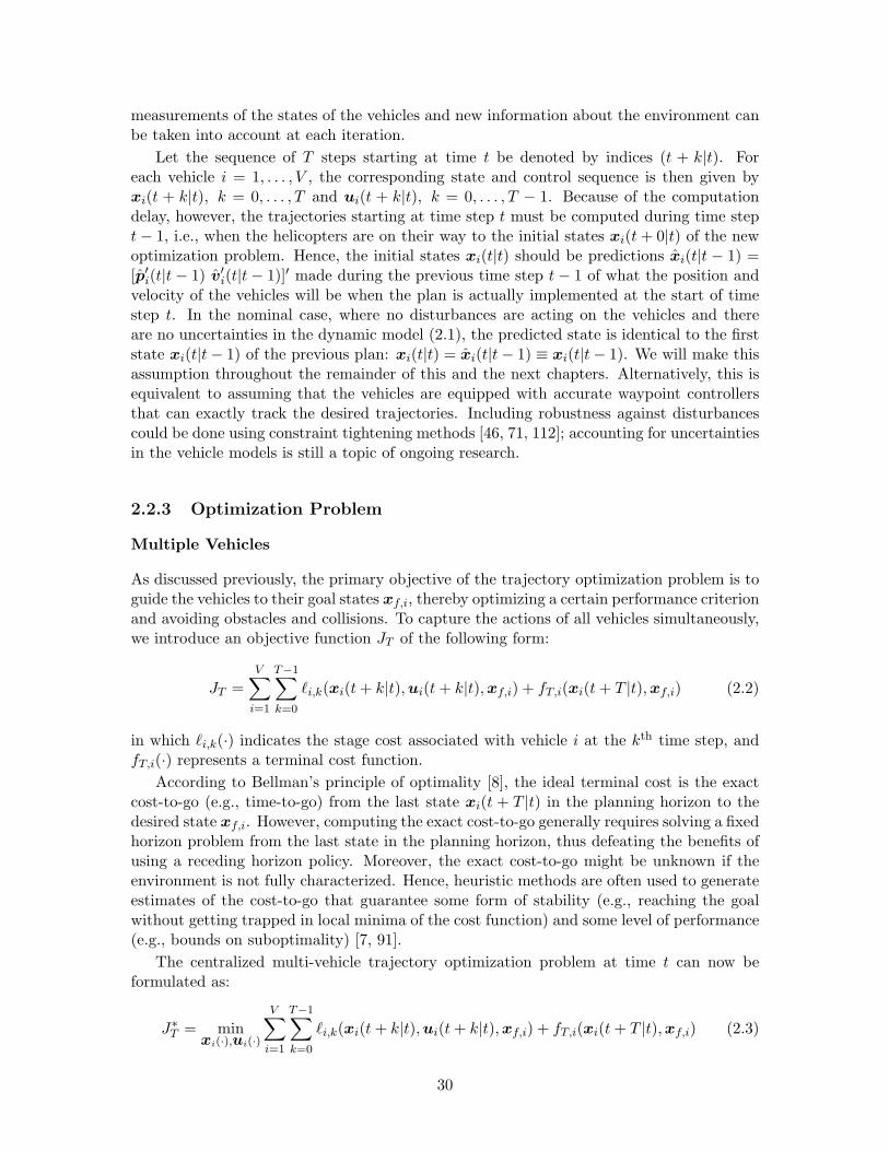
As discussed previously, the primary objective of the trajectory optimization problem is toguide the vehicles to their goal states xf,i, thereby optimizing a certain performance criterionand avoiding obstacles and collisions. To capture the actions of all vehicles simultaneously,we introduce an objective function JT of the following form:
JT =V
∑
i=1
T−1∑
k=0
ℓi,k(xi(t + k|t), ui(t + k|t), xf,i) + fT,i(xi(t + T |t), xf,i) (2.2)
in which ℓi,k(·) indicates the stage cost associated with vehicle i at the kth time step, andfT,i(·) represents a terminal cost function.
According to Bellman’s principle of optimality [8], the ideal terminal cost is the exactcost-to-go (e.g., time-to-go) from the last state xi(t + T |t) in the planning horizon to thedesired state xf,i. However, computing the exact cost-to-go generally requires solving a fixedhorizon problem from the last state in the planning horizon, thus defeating the benefits ofusing a receding horizon policy. Moreover, the exact cost-to-go might be unknown if theenvironment is not fully characterized. Hence, heuristic methods are often used to generateestimates of the cost-to-go that guarantee some form of stability (e.g., reaching the goalwithout getting trapped in local minima of the cost function) and some level of performance(e.g., bounds on suboptimality) [7, 91].
The centralized multi-vehicle trajectory optimization problem at time t can now beformulated as:
J∗T = min
xi(·),ui(·)
V∑
i=1
T−1∑
k=0
ℓi,k(xi(t + k|t), ui(t + k|t), xf,i) + fT,i(xi(t + T |t), xf,i) (2.3)
30
subject to: ∀i = 1, . . . , V :
xi(t + k + 1|t) = Aixi(t + k|t) + Biui(t + k|t), k = 0, . . . , T − 1 (2.4)
xi(t|t) = xi(t|t − 1) (2.5)
xi(t + k|t) ∈ Xi(k), k = 1, . . . , T (2.6)
ui(t + k|t) ∈ Ui(k), k = 0, . . . , T − 1 (2.7)
pi(t + k|t) /∈ Oa,i(t), k = 1, . . . , T (2.8)
‖pi(t + k|t) − pj(t + k|t)‖ ≥ dsafe, j ≥ i + 1, k = 1, . . . , T (2.9)
Since the problem only makes sense if the initial states xi(t|t) are feasible, the state con-straints on the first time step were removed: if they did not hold, the optimization problemwould be infeasible from the start. Furthermore, to prevent the discrete-time trajectoriesfrom cutting corners of obstacles in between two time steps, the obstacle sets Oa,i containthe actual obstacles enlarged with a safety envelope. The trajectories may then cut throughthe envelope instead, but will avoid the actual obstacles.
Single Vehicle
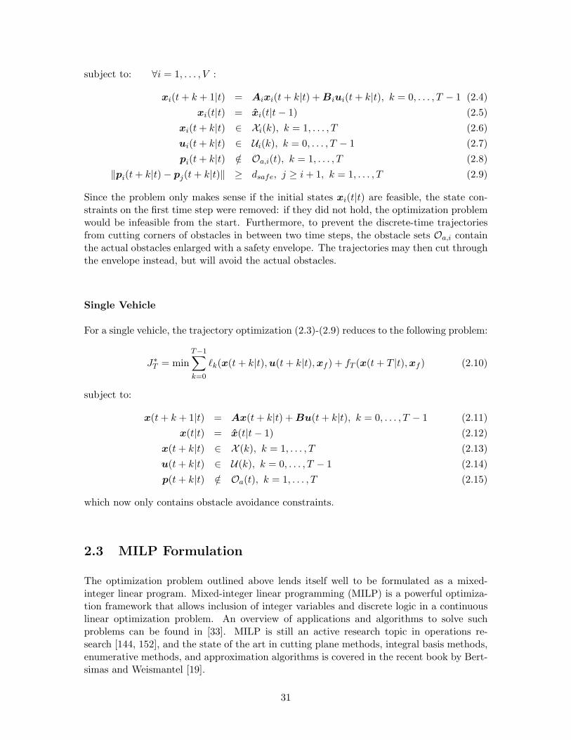
For a single vehicle, the trajectory optimization (2.3)-(2.9) reduces to the following problem:
J∗T = min
T−1∑
k=0
ℓk(x(t + k|t), u(t + k|t), xf ) + fT (x(t + T |t), xf ) (2.10)
subject to:
x(t + k + 1|t) = Ax(t + k|t) + Bu(t + k|t), k = 0, . . . , T − 1 (2.11)
x(t|t) = x(t|t − 1) (2.12)
x(t + k|t) ∈ X (k), k = 1, . . . , T (2.13)
u(t + k|t) ∈ U(k), k = 0, . . . , T − 1 (2.14)
p(t + k|t) /∈ Oa(t), k = 1, . . . , T (2.15)
which now only contains obstacle avoidance constraints.
2.3 MILP Formulation
The optimization problem outlined above lends itself well to be formulated as a mixed-integer linear program. Mixed-integer linear programming (MILP) is a powerful optimiza-tion framework that allows inclusion of integer variables and discrete logic in a continuouslinear optimization problem. An overview of applications and algorithms to solve suchproblems can be found in [33]. MILP is still an active research topic in operations re-search [144, 152], and the state of the art in cutting plane methods, integral basis methods,enumerative methods, and approximation algorithms is covered in the recent book by Bert-simas and Weismantel [19].
31
2.3.1 Mixed Integer Linear Programming
As an illustration of how logical decisions can be incorporated in an optimization problem,consider the following example. Assume that a cost function J(x) needs to be minimizedsubject to either one of two constraints ℓ1(x) and ℓ2(x) on the continuous decision vectorx:
minx
J(x)
subject to:ℓ1(x) ≤ 0
OR ℓ2(x) ≤ 0
(2.16)
By introducing a large positive number M and a binary variable b, this optimization problemcan equivalently be formulated as follows:
minx
J(x)
subject to:ℓ1(x) ≤ Mb
AND ℓ2(x) ≤ M(1 − b)b ∈ {0, 1}
(2.17)
When b = 0, constraint ℓ1(x) must be satisfied, whereas ℓ2(x) is relaxed. Namely, if Mis chosen sufficiently large, ℓ2(x) ≤ M(1 − b) is always satisfied independent of the valueof x. The situation is reversed when b = 1. Since b can only take the binary values 0 or1, at least one of the constraints ℓ1(x) and ℓ2(x) will be satisfied, which is equivalent tothe original “OR”-formulation (2.16). In the special case where J(x), ℓ1(x) and ℓ2(x) are(affine) linear expressions, problem (2.17) is a MILP.
The formulation can easily be extended to account for multiple constraints ℓk(x), k =1, . . . , K, out of which at least N must be satisfied simultaneously. This is done as follows:
minx
J(x)
subject to:ℓk(x) ≤ Mbk, k = 1, . . . , K∑
k
bk ≤ K − N
bk ∈ {0, 1}
(2.18)
The additional summation constraint ensures that at least N of the binary variables bk are 0,thus guaranteeing that at least N of the inequalities ℓk(x) ≤ 0 are satisfied simultaneously.More generally, using a vector b of binary variables, any polyhedron or intersection ofpolyhedra described by linear constraints on a continuous decision vector x can then bedescribed as follows:
Lx + Mb + k ≤ 0 (2.19)
The constant matrix M and vector k contain large numbers M and integer constants Kand N that can encode any binary logic such as that of problem (2.18).
2.3.2 Vehicle Dynamics
In the trajectory planning problem, the continuous optimization is done over the statesand inputs, while binary variables are introduced to capture non-convex constraints such
32
y
x
v
vmax
vmin
•
•
Figure 2-1: Approximation of minimum and maximum velocity bounds by polygons.
as obstacle avoidance, collision avoidance and minimum velocity requirements. Since thestructure of the optimization problem is the same at every receding horizon iteration, inwhat follows, we will shorten the time step index (t + k|k) to k to simplify the notation.
Although it is possible to use more complicated models, for the basic problem presentedin this chapter, it is sufficient to approximate the vehicle dynamics by a double integratormodel with constraints on speed and acceleration. Alternative models will be introducedin later chapters. The 3D discrete-time, unconstrained double integrator dynamics used fornow are the following:
[
pi(k + 1)vi(k + 1)
]
=
[
I3 ∆tI3
O3 I3
] [
pi(k)vi(k)
]
+
[
(∆t)2
2 I3
∆tI3
]
ai(k) (2.20)
where ai(k) ≡ [xi(k) yi(k) zi(k)]′ is the inertial acceleration vector, ∆t is the time dis-cretization step, and I3 and O3 represent identity and zero matrices of size 3x3.
We use the above dynamic model for both fixed-wing aircraft and rotorcraft scenarios.In the fixed-wing case, however, we will only consider 2D scenarios with corresponding 2Ddouble integrator dynamics. Limiting the magnitude of the planar velocity and acceler-ation vectors can then be accomplished by approximating their 2-norms ‖[xi(k) yi(k)]′‖and ‖[xi(k) yi(k)]′‖ by the edges of an N -sided polygon (see Figure 2-1). This yields thefollowing set of linear inequalities:
xi(k) sin
(
2πn
N
)
+ yi(k) cos
(
2πn
N
)
≤ vmax,i, n = 1, . . . , N, k = 1, . . . , T (2.21)
xi(k) sin
(
2πn
N
)
+ yi(k) cos
(
2πn
N
)
≤ amax,i, n = 1, . . . , N, k = 0, . . . , T − 1(2.22)
For coordinated turns, inequalities (2.22) also implicitly express a constraint on the maxi-mum turn rate ωmax,i: it is limited to amax,i/vmax,i at the maximum speed and to amax,i/vmin,i
at the minimum speed [114].
Since a fixed-wing aircraft has to produce enough lift to keep flying, it must maintaina minimum velocity vmin. As shown in Figure 2-1, this requirement can be expressed by
33
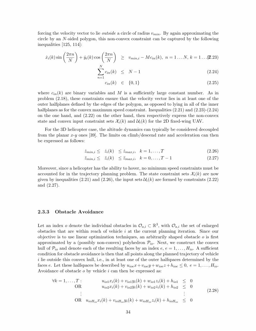
forcing the velocity vector to lie outside a circle of radius vmin. By again approximating thecircle by an N -sided polygon, this non-convex constraint can be captured by the followinginequalities [125, 114]:
xi(k) sin
(
2πn
N
)
+ yi(k) cos
(
2πn
N
)
≥ vmin,i − Mcin(k), n = 1 . . . N, k = 1 . . . T(2.23)
N∑
n=1
cin(k) ≤ N − 1 (2.24)
cin(k) ∈ {0, 1} (2.25)
where cin(k) are binary variables and M is a sufficiently large constant number. As inproblem (2.18), these constraints ensure that the velocity vector lies in at least one of theouter halfplanes defined by the edges of the polygon, as opposed to lying in all of the innerhalfplanes as for the convex maximum speed constraint. Inequalities (2.21) and (2.23)-(2.24)on the one hand, and (2.22) on the other hand, then respectively express the non-convexstate and convex input constraint sets Xi(k) and Ui(k) for the 2D fixed-wing UAV.
For the 3D helicopter case, the altitude dynamics can typically be considered decoupledfrom the planar x-y ones [39]. The limits on climb/descend rate and acceleration can thenbe expressed as follows:
zmin,i ≤ zi(k) ≤ zmax,i, k = 1, . . . , T (2.26)
zmin,i ≤ zi(k) ≤ zmax,i, k = 0, . . . , T − 1 (2.27)
Moreover, since a helicopter has the ability to hover, no minimum speed constraints must beaccounted for in the trajectory planning problem. The state constraint sets Xi(k) are nowgiven by inequalities (2.21) and (2.26), the input sets Ui(k) are formed by constraints (2.22)and (2.27).
2.3.3 Obstacle Avoidance
Let an index o denote the individual obstacles in Oa,i ⊂ R3, with Oa,i the set of enlarged
obstacles that are within reach of vehicle i at the current planning iteration. Since ourobjective is to use linear optimization techniques, an arbitrarily shaped obstacle o is firstapproximated by a (possibly non-convex) polyhedron Pio. Next, we construct the convexhull of Pio and denote each of the resulting faces by an index e, e = 1, . . . , Hio. A sufficientcondition for obstacle avoidance is then that all points along the planned trajectory of vehiclei lie outside this convex hull, i.e., in at least one of the outer halfspaces determined by thefaces e. Let these halfspaces be described by uioex+vioey+wioez +hioe ≤ 0, e = 1, . . . , Hio.Avoidance of obstacle o by vehicle i can then be expressed as:
∀k = 1, . . . , T : uio1xi(k) + vio1yi(k) + wio1zi(k) + hio1 ≤ 0OR uio2xi(k) + vio2yi(k) + wio2zi(k) + hio2 ≤ 0
......
OR uioHioxi(k) + vioHio
yi(k) + wioHiozi(k) + hioHio
≤ 0
(2.28)
34
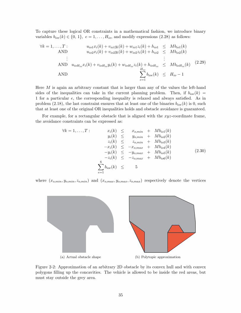
To capture these logical OR constraints in a mathematical fashion, we introduce binaryvariables bioe(k) ∈ {0, 1}, e = 1, . . . , Hio, and modify expressions (2.28) as follows:
∀k = 1, . . . , T : uio1xi(k) + vio1yi(k) + wio1zi(k) + hio1 ≤ Mbio1(k)AND uio2xi(k) + vio2yi(k) + wio2zi(k) + hio2 ≤ Mbio2(k)
......
AND uioHioxi(k) + vioHio
yi(k) + wioHiozi(k) + hioHio
≤ MbioHio(k)
AND
Hio∑
e=1
bioe(k) ≤ Hio − 1
(2.29)
Here M is again an arbitrary constant that is larger than any of the values the left-handsides of the inequalities can take in the current planning problem. Then, if bioe(k) =1 for a particular e, the corresponding inequality is relaxed and always satisfied. As inproblem (2.18), the last constraint ensures that at least one of the binaries bioe(k) is 0, suchthat at least one of the original OR inequalities holds and obstacle avoidance is guaranteed.
For example, for a rectangular obstacle that is aligned with the xyz-coordinate frame,the avoidance constraints can be expressed as:
∀k = 1, . . . , T : xi(k) ≤ xo,min + Mbio1(k)yi(k) ≤ yo,min + Mbio2(k)zi(k) ≤ zo,min + Mbio3(k)
−xi(k) ≤ −xo,max + Mbio4(k)−yi(k) ≤ −yo,max + Mbio5(k)−zi(k) ≤ −zo,max + Mbio6(k)
6∑
e=1
bioe(k) ≤ 5
(2.30)
where (xo,min, yo,min, zo,min) and (xo,max, yo,max, zo,max) respectively denote the vertices
(a) Actual obstacle shape (b) Polytopic approximation
Figure 2-2: Approximation of an arbitrary 2D obstacle by its convex hull and with convexpolygons filling up the concavities. The vehicle is allowed to be inside the red areas, butmust stay outside the grey area.
35
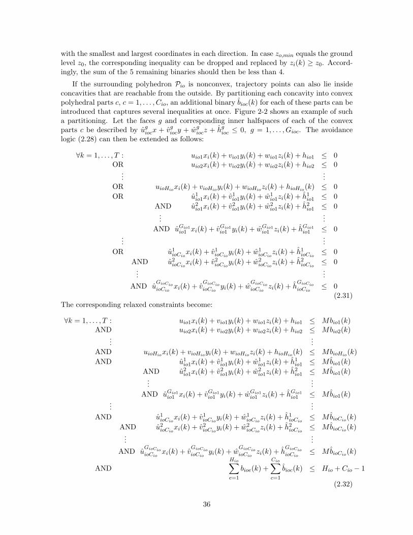
with the smallest and largest coordinates in each direction. In case zo,min equals the groundlevel z0, the corresponding inequality can be dropped and replaced by zi(k) ≥ z0. Accord-ingly, the sum of the 5 remaining binaries should then be less than 4.
If the surrounding polyhedron Pio is nonconvex, trajectory points can also lie insideconcavities that are reachable from the outside. By partitioning each concavity into convexpolyhedral parts c, c = 1, . . . , Cio, an additional binary bioc(k) for each of these parts can beintroduced that captures several inequalities at once. Figure 2-2 shows an example of sucha partitioning. Let the faces g and corresponding inner halfspaces of each of the convexparts c be described by ug
iocx + vgiocy + wg
iocz + hgioc ≤ 0, g = 1, . . . , Gioc. The avoidance
logic (2.28) can then be extended as follows:
∀k = 1, . . . , T : uio1xi(k) + vio1yi(k) + wio1zi(k) + hio1 ≤ 0OR uio2xi(k) + vio2yi(k) + wio2zi(k) + hio2 ≤ 0
......
OR uioHioxi(k) + vioHio
yi(k) + wioHiozi(k) + hioHio
(k) ≤ 0
OR u1io1xi(k) + v1
io1yi(k) + w1io1zi(k) + h1
io1 ≤ 0
AND u2io1xi(k) + v2
io1yi(k) + w2io1zi(k) + h2
io1 ≤ 0...
...
AND uGio1
io1 xi(k) + vGio1
io1 yi(k) + wGio1
io1 zi(k) + hGio1
io1 ≤ 0...
...
OR u1ioCio
xi(k) + v1ioCio
yi(k) + w1ioCio
zi(k) + h1ioCio
≤ 0
AND u2ioCio
xi(k) + v2ioCio
yi(k) + w2ioCio
zi(k) + h2ioCio
≤ 0...
...
AND uGioCio
ioCioxi(k) + v
GioCio
ioCioyi(k) + w
GioCio
ioCiozi(k) + h
GioCio
ioCio≤ 0
(2.31)The corresponding relaxed constraints become:
∀k = 1, . . . , T : uio1xi(k) + vio1yi(k) + wio1zi(k) + hio1 ≤ Mbio1(k)AND uio2xi(k) + vio2yi(k) + wio2zi(k) + hio2 ≤ Mbio2(k)
......
AND uioHioxi(k) + vioHio
yi(k) + wioHiozi(k) + hioHio
(k) ≤ MbioHio(k)
AND u1io1xi(k) + v1
io1yi(k) + w1io1zi(k) + h1
io1 ≤ Mbio1(k)
AND u2io1xi(k) + v2
io1yi(k) + w2io1zi(k) + h2
io1 ≤ Mbio1(k)...
...
AND uGio1
io1 xi(k) + vGio1
io1 yi(k) + wGio1
io1 zi(k) + hGio1
io1 ≤ Mbio1(k)...
...
AND u1ioCio
xi(k) + v1ioCio
yi(k) + w1ioCio
zi(k) + h1ioCio
≤ MbioCio(k)
AND u2ioCio
xi(k) + v2ioCio
yi(k) + w2ioCio
zi(k) + h2ioCio
≤ MbioCio(k)
......
AND uGioCio
ioCioxi(k) + v
GioCio
ioCioyi(k) + w
GioCio
ioCiozi(k) + h
GioCio
ioCio≤ MbioCio
(k)
AND
Hio∑
e=1
bioe(k) +
Cio∑
c=1
bioc(k) ≤ Hio + Cio − 1
(2.32)
36
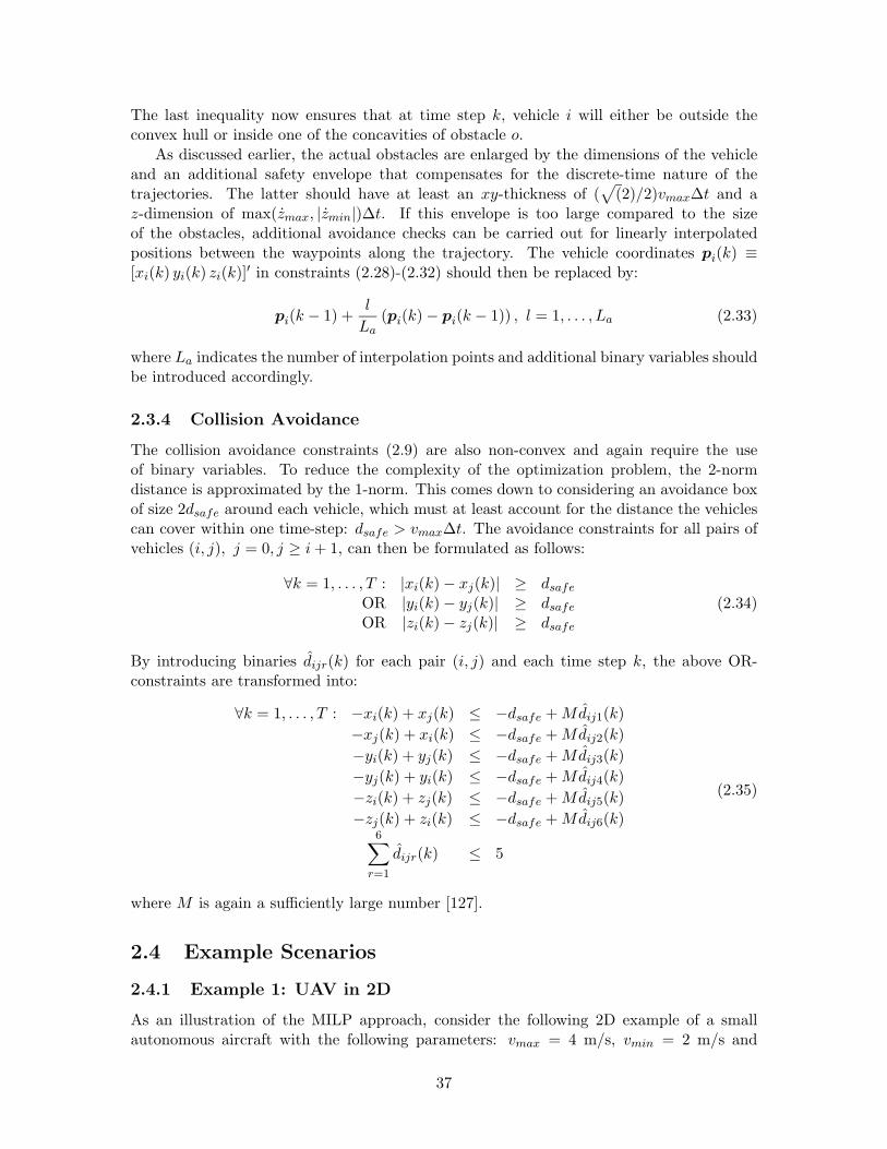
The last inequality now ensures that at time step k, vehicle i will either be outside theconvex hull or inside one of the concavities of obstacle o.
As discussed earlier, the actual obstacles are enlarged by the dimensions of the vehicleand an additional safety envelope that compensates for the discrete-time nature of thetrajectories. The latter should have at least an xy-thickness of (
√
(2)/2)vmax∆t and az-dimension of max(zmax, |zmin|)∆t. If this envelope is too large compared to the sizeof the obstacles, additional avoidance checks can be carried out for linearly interpolatedpositions between the waypoints along the trajectory. The vehicle coordinates pi(k) ≡[xi(k) yi(k) zi(k)]′ in constraints (2.28)-(2.32) should then be replaced by:
pi(k − 1) +l
La
(pi(k) − pi(k − 1)) , l = 1, . . . , La (2.33)
where La indicates the number of interpolation points and additional binary variables shouldbe introduced accordingly.
2.3.4 Collision Avoidance
The collision avoidance constraints (2.9) are also non-convex and again require the useof binary variables. To reduce the complexity of the optimization problem, the 2-normdistance is approximated by the 1-norm. This comes down to considering an avoidance boxof size 2dsafe around each vehicle, which must at least account for the distance the vehiclescan cover within one time-step: dsafe > vmax∆t. The avoidance constraints for all pairs ofvehicles (i, j), j = 0, j ≥ i + 1, can then be formulated as follows:
∀k = 1, . . . , T : |xi(k) − xj(k)| ≥ dsafe
OR |yi(k) − yj(k)| ≥ dsafe
OR |zi(k) − zj(k)| ≥ dsafe
(2.34)
By introducing binaries dijr(k) for each pair (i, j) and each time step k, the above OR-constraints are transformed into:
∀k = 1, . . . , T : −xi(k) + xj(k) ≤ −dsafe + Mdij1(k)
−xj(k) + xi(k) ≤ −dsafe + Mdij2(k)
−yi(k) + yj(k) ≤ −dsafe + Mdij3(k)
−yj(k) + yi(k) ≤ −dsafe + Mdij4(k)
−zi(k) + zj(k) ≤ −dsafe + Mdij5(k)
−zj(k) + zi(k) ≤ −dsafe + Mdij6(k)6
∑
r=1
dijr(k) ≤ 5
(2.35)
where M is again a sufficiently large number [127].
2.4 Example Scenarios
2.4.1 Example 1: UAV in 2D
As an illustration of the MILP approach, consider the following 2D example of a smallautonomous aircraft with the following parameters: vmax = 4 m/s, vmin = 2 m/s and
37
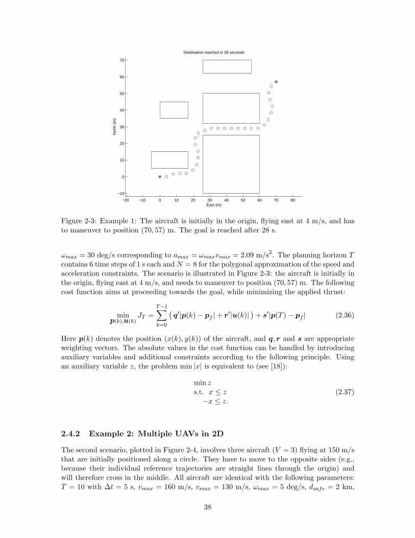
−20 −10 0 10 20 30 40 50 60 70 80
−10
0
10
20
30
40
50
60
70
Destination reached in 28 seconds
East (m)
Nor
th (
m)
Figure 2-3: Example 1: The aircraft is initially in the origin, flying east at 4 m/s, and hasto maneuver to position (70, 57) m. The goal is reached after 28 s.
ωmax = 30 deg/s corresponding to amax = ωmaxvmax = 2.09 m/s2. The planning horizon Tcontains 6 time steps of 1 s each and N = 8 for the polygonal approximation of the speed andacceleration constraints. The scenario is illustrated in Figure 2-3: the aircraft is initially inthe origin, flying east at 4 m/s, and needs to maneuver to position (70, 57) m. The followingcost function aims at proceeding towards the goal, while minimizing the applied thrust:
minp(k),u(k)
JT =
T−1∑
k=0
(
q′|p(k) − pf | + r′|u(k)|)
+ s′|p(T ) − pf | (2.36)
Here p(k) denotes the position (x(k), y(k)) of the aircraft, and q, r and s are appropriateweighting vectors. The absolute values in the cost function can be handled by introducingauxiliary variables and additional constraints according to the following principle. Usingan auxiliary variable z, the problem min |x| is equivalent to (see [18]):
min zs.t. x ≤ z
−x ≤ z.(2.37)
2.4.2 Example 2: Multiple UAVs in 2D
The second scenario, plotted in Figure 2-4, involves three aircraft (V = 3) flying at 150 m/sthat are initially positioned along a circle. They have to move to the opposite sides (e.g.,because their individual reference trajectories are straight lines through the origin) andwill therefore cross in the middle. All aircraft are identical with the following parameters:T = 10 with ∆t = 5 s, vmax = 160 m/s, vmax = 130 m/s, ωmax = 5 deg/s, dsafe = 2 km,
38
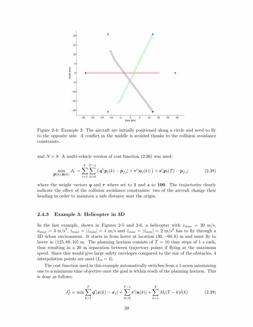
−25 −20 −15 −10 −5 0 5 10 15 20 25
−20
−15
−10
−5
0
5
10
15
20
East (km)
Nor
th (
km)
Figure 2-4: Example 2: The aircraft are initially positioned along a circle and need to flyto the opposite side. A conflict in the middle is avoided thanks to the collision avoidanceconstraints.
and N = 8. A multi-vehicle version of cost function (2.36) was used:
minp(k),u(k)
JV =
V∑
i=1
T−1∑
k=0
(
q′|pi(k) − pf,i| + r′|ui(k)|)
+ s′|pi(T ) − pf,i| (2.38)
where the weight vectors q and r where set to 1 and s to 100. The trajectories clearlyindicate the effect of the collision avoidance constraints: two of the aircraft change theirheading in order to maintain a safe distance near the origin.
2.4.3 Example 3: Helicopter in 3D
In the last example, shown in Figures 2-5 and 2-6, a helicopter with vmax = 20 m/s,amax = 3 m/s2, zmax = |zmin| = 4 m/s and zmax = |zmin| = 2 m/s2 has to fly through a3D urban environment. It starts in from hover at location (30,−60, 8) m and must fly tohover in (125, 60, 10) m. The planning horizon consists of T = 10 time steps of 1 s each,thus resulting in a 20 m separation between trajectory points if flying at the maximumspeed. Since this would give large safety envelopes compared to the size of the obstacles, 4interpolation points are used (La = 4).
The cost function used in this example automatically switches from a 1-norm minimizingone to a minimum time objective once the goal is within reach of the planning horizon. Thisis done as follows:
J∗T = min
T∑
k=1
q′|x(k) − xf | +T−1∑
k=0
r′|u(k)| +T
∑
k=1
Mt(T − k)t(k) (2.39)
39
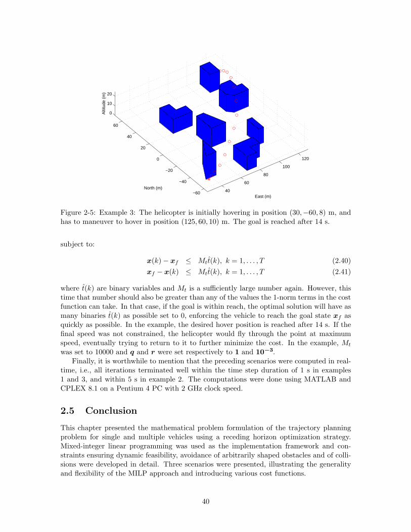
40
60
80
100
120
−60
−40
−20
0
20
40
60
0
10
20
East (m)
North (m)
Alti
tude
(m
)
Figure 2-5: Example 3: The helicopter is initially hovering in position (30,−60, 8) m, andhas to maneuver to hover in position (125, 60, 10) m. The goal is reached after 14 s.
subject to:
x(k) − xf ≤ Mtt(k), k = 1, . . . , T (2.40)
xf − x(k) ≤ Mtt(k), k = 1, . . . , T (2.41)
where t(k) are binary variables and Mt is a sufficiently large number again. However, thistime that number should also be greater than any of the values the 1-norm terms in the costfunction can take. In that case, if the goal is within reach, the optimal solution will have asmany binaries t(k) as possible set to 0, enforcing the vehicle to reach the goal state xf asquickly as possible. In the example, the desired hover position is reached after 14 s. If thefinal speed was not constrained, the helicopter would fly through the point at maximumspeed, eventually trying to return to it to further minimize the cost. In the example, Mt
was set to 10000 and q and r were set respectively to 1 and 10−3.Finally, it is worthwhile to mention that the preceding scenarios were computed in real-
time, i.e., all iterations terminated well within the time step duration of 1 s in examples1 and 3, and within 5 s in example 2. The computations were done using MATLAB andCPLEX 8.1 on a Pentium 4 PC with 2 GHz clock speed.
2.5 Conclusion
This chapter presented the mathematical problem formulation of the trajectory planningproblem for single and multiple vehicles using a receding horizon optimization strategy.Mixed-integer linear programming was used as the implementation framework and con-straints ensuring dynamic feasibility, avoidance of arbitrarily shaped obstacles and of colli-sions were developed in detail. Three scenarios were presented, illustrating the generalityand flexibility of the MILP approach and introducing various cost functions.
40
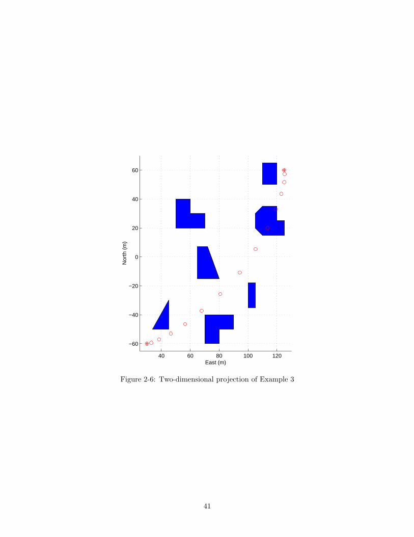
40 60 80 100 120
−60
−40
−20
0
20
40
60
East (m)
Nor
th (
m)
Figure 2-6: Two-dimensional projection of Example 3
41

42

Chapter 3
Hybrid Model for Agile Vehicles
This chapter presents a hybrid model and control architecture for trajectory planning ofagile vehicles. A velocity control system providing the ability to accurately track trajectoriesis combined with a maneuver scheduler that enables execution of pre-programmed agilemaneuvers. The closed-loop dynamics under this control architecture are described by asimple hybrid model, consisting of a set of constrained, linear time-invariant modes anddiscrete fixed-duration transitions in the state space. Given these dynamics, mixed-integerlinear programming is again used to compute optimal trajectories in cluttered environments.Continuous constraints and binary logic are combined to model the constraints governingthe dynamics, to formulate switching rules between different velocity modes, to encodeexecution of agile maneuvers, and to account for obstacle avoidance. Both offline time-optimal planning and online receding horizon formulations are presented. The frameworkis applied in detail to a small-scale helicopter, for which several receding horizon results aregiven. A discussion about practical considerations regarding a real-time implementationconcludes the chapter.
3.1 Introduction
Taking advantage of the full range of vehicle maneuverability in an autonomous fashion iskey to a number of potential UAV tasks. Examples include tracking of moving targets, flyingthrough cluttered (e.g., urban) environments, and tactical flight, such as nap of the earth.In these applications, autonomous agile maneuvering can either be necessary – for instanceto effectively avoid pop-up obstacles– or may represent a competitive advantage. However,as discussed earlier, it is known that motion planning is intrinsically PSPACE-hard [110, 49]and that its complexity grows with that of the vehicle dynamics and the environment inwhich the vehicle has to operate. For vehicles with fast and complex dynamics, such as small-scale rotorcraft [43], it is therefore impractical to consider the full equations of motion inthe development of an autonomous trajectory planning system. For such vehicles, the statespace and the set of possible control actions are extremely large, requiring simplificationsto reduce the dimensionality when a solution has to be computed in real-time.
A well-established idea to reduce the complexity is to first organize the vehicle dynamicsthrough some form of control augmentation, such as velocity controllers, and to then designthe guidance system using the simpler closed-loop dynamics. However, for highly agilevehicles, such an approach might restrict the performance. An alternative method is touse a “maneuver automaton” as was introduced by Frazzoli et al. [36]. The framework
43
was later applied to an X-Cell miniature helicopter as described in [93] and [128]. Withthis approach, the vehicle is modeled as a hybrid automaton, consisting of a set of discreteequilibrium trim conditions and transitions between these trims, called maneuvers. Bychoosing an appropriate set of such motion primitives, the state space can be significantlyreduced without giving up the key performance and maneuverability of the vehicle. Optimaltrajectories are obtained in real-time by evaluating the possible discrete actions at each timestep, i.e., to stay on the current trim trajectory or to execute a maneuver. The decision ismade according to an optimal policy operating on a value function, which results from adynamic program that is solved offline by value iteration [17].
The maneuver automaton as described above, however, has several drawbacks. Theseare primarily related to the fact that the vehicle dynamics are constrained to a finite set ofmotion primitives. Namely, velocity is discretized into several trims with constant speeds,thus restricting the vehicle’s behavior to one of these. The lack of continuous velocity modesand the discretization used in the value function can be a problem when precise navigationis required, as illustrated by our results in [93, 128]. Moreover, since one operating region istypically discretized into multiple trim conditions with corresponding transition maneuvers,the complexity of the maneuver automaton and corresponding dynamic program increasessignificantly with the resolution of the discretization.
This chapter presents an alternative approach based on a hybrid architecture that com-bines a velocity control system and a maneuver scheduler. Using this framework, opti-mal trajectory design can again be formulated as a mixed-integer linear program. Besidesallowing for obstacle and collision avoidance, in this specific case, MILP is used to opti-mally switch between various velocity control modes and to incorporate the binary decisionswhether or not to execute a maneuver. As such, this chapter extends the basic trajectoryplanning formulation presented in Chapter 2 by accounting for more agile dynamics thanthe ones used before. We will specialize the approach to the case of a small-scale rotorcraftusing a MILP model based on MIT’s aerobatic X-Cell helicopter.
The chapter is organized as follows. Section 3.2 presents the hybrid control architectureand a corresponding high-level dynamic model. Given these dynamics, Section 3.3 outlinesthe use of MILP for optimal guidance. In Section 3.4, the framework is applied to guidance ofa small-scale helicopter, for which simulation results are presented in Section 3.5. Section 3.6then discusses some practical considerations regarding a real-time implementation.
3.2 Hybrid Control Architecture for Guidance
3.2.1 Automatic Control of Agile Vehicles
The control architecture presented in this chapter is based on the analysis of human controlof highly agile, small-scale helicopters [40]. It shows two distinct operating regimes: trackingof trim trajectories and maneuvering. The two modes are distinctly set apart in terms ofcontrol strategy and dynamic conditions:
• Tracking operations take place around trim trajectories. Control around these trajec-tories involves continuous feedback, and the dynamics are approximately linear.
• Maneuvering actions are of finite duration and start and end on trim trajectories.The control activity typically involves large amplitude input commands that exploitthe extreme performance of the vehicle and result in large changes of its state. The
44
dynamics across this range are typically nonlinear. Control is dominated by feed-forward actions; feedback may include discrete switching events triggered by statethresholds.
Tracking trim trajectories is a well-researched area; automatic maneuvering, however,is more challenging due the highly nonlinear dynamics [48]. Instead of applying traditionalnonlinear control methods such as feedback linearization [140], a control logic inspiredby the above human strategies was recently developed for an autonomous miniature heli-copter [44]. It combines angular rate controllers and a timing logic that enables trackingof pre-programmed reference trajectories. The amplitude and timing of these trajectoriesor maneuvers were extracted from piloted flight-test experiments. Prior to and upon exitfrom a maneuver, gain-scheduled linear quadratic trim tracking controllers are used. Usingthis approach, several aerobatic maneuvers were successfully implemented, including a snaproll, a hammerhead, and a split-S [41].
A block diagram of the switching control architecture is shown in Figure 3-1. Thevelocity controllers enable the vehicle to accurately track trajectories throughout a largeregion of the flight envelope, whereas the maneuvers take the helicopter through its extremerange of performance. Under this control architecture, the closed-loop dynamics of the agilevehicle can be accurately described by a combination of low-order, linear time-invariant(LTI) equations of motion and discrete state transitions. An abstract representation of thisstructure is given in Figure 3-2: it shows that maneuvers start and end in the linear velocitycontrol regime.
More generally, for any type of unmanned agile vehicle, the combination of gain-scheduledLTI modes and a finite number of fast, pre-programmed maneuvers enables a broad range ofbehaviors that can be exploited when designing mission-specific trajectories. The benefitsof this approach are several. First, the model allows for precise navigation in the veloc-ity control mode, without compromising on agility when extreme transitions are required,such as during reactive threat or obstacle avoidance. Second, compared to the maneuverautomaton approach [36], the architecture significantly simplifies the development of a mo-tion primitive library: the problem is reduced to selecting a few LTI modes and a smallset of agile maneuvers. In what follows, we formalize this control structure in a mathe-matical framework, which can then be used to effectively formulate trajectory optimizationproblems.
3.2.2 Velocity Control System
Assume that the gain-scheduled velocity controllers result in L distinct, mutually exclusiveLTI modes or operating regions. In general, each LTI mode l corresponds to a discrete-time state space model x(k + 1) = Alx(k) + Blu(k) in some vector space R
ns , where theindex k again indicates the discrete time step. As was discussed in Chapter 2, the statevector x ∈ R
ns typically contains velocity and position components in either a body-fixedand/or inertial coordinate frame. The input vector u ∈ R
nu generally consists of referencevelocity commands or accelerations, again in either coordinate frame. The key requirementis that the state space models describe the closed-loop dynamics of the vehicle in a formthat is compatible with the type of desired guidance. For example, if a waypoint follower isavailable, a closed-loop model incorporating this controller could be considered that takesinertial positions as inputs. Alternatively, it may be desirable to directly steer the vehicleusing body-fixed frame velocity commands. Since the formulation that we will present can
45
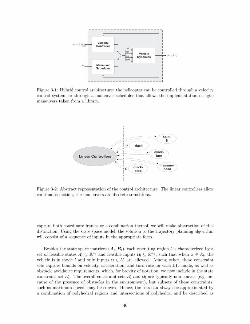
Figure 3-1: Hybrid control architecture: the helicopter can be controlled through a velocitycontrol system, or through a maneuver scheduler that allows the implementation of agilemaneuvers taken from a library.
Linear Controllers
hammer-head
split-S
quick-turn
dash
quick-stop
Figure 3-2: Abstract representation of the control architecture. The linear controllers allowcontinuous motion, the maneuvers are discrete transitions.
capture both coordinate frames or a combination thereof, we will make abstraction of thisdistinction. Using the state space model, the solution to the trajectory planning algorithmwill consist of a sequence of inputs in the appropriate form.
Besides the state space matrices (Al, Bl), each operating region l is characterized by aset of feasible states Xl ⊆ R
ns and feasible inputs Ul ⊆ Rnu , such that when x ∈ Xl, the
vehicle is in mode l and only inputs u ∈ Ul are allowed. Among other, these constraintsets capture bounds on velocity, acceleration, and turn rate for each LTI mode, as well asobstacle avoidance requirements, which, for brevity of notation, we now include in the stateconstraint set Xl. The overall constraint sets Xl and Ul are typically non-convex (e.g. be-cause of the presence of obstacles in the environment), but subsets of these constraints,such as maximum speed, may be convex. Hence, the sets can always be approximated bya combination of polyhedral regions and intersections of polyhedra, and be described as
46
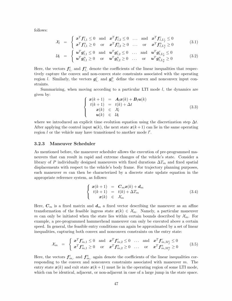
follows:
Xl =
{
xT f cl,1 ≤ 0 and xT f c
l,2 ≤ 0 . . . and xT f cl,Lc
f≤ 0
xT fnl,1 ≥ 0 or xT fn
l,2 ≥ 0 . . . or xT fnl,Ln
f≥ 0
(3.1)
Ul =
{
uT gcl,1 ≤ 0 and uT gc
l,2 ≤ 0 . . . and uT gcl,Lc
g≤ 0
uT gnl,1 ≥ 0 or uT gn
l,2 ≥ 0 . . . or uT gnl,Ln
g≥ 0
(3.2)
Here, the vectors f cl,· and fn
l,· denote the coefficients of the linear inequalities that respec-tively capture the convex and non-convex state constraints associated with the operatingregion l. Similarly, the vectors gc
l,· and gnl,· define the convex and nonconvex input con-
straints.
Summarizing, when moving according to a particular LTI mode l, the dynamics aregiven by:
x(k + 1) = Alx(k) + Blu(k)t(k + 1) = t(k) + ∆t
x(k) ∈ Xl
u(k) ∈ Ul
(3.3)
where we introduced an explicit time evolution equation using the discretization step ∆t.After applying the control input u(k), the next state x(k +1) can lie in the same operatingregion l or the vehicle may have transitioned to another mode l′.
3.2.3 Maneuver Scheduler
As mentioned before, the maneuver scheduler allows the execution of pre-programmed ma-neuvers that can result in rapid and extreme changes of the vehicle’s state. Consider alibrary of P individually designed maneuvers with fixed durations ∆Tm and fixed spatialdisplacements with respect to the vehicle’s body frame. For trajectory planning purposes,each maneuver m can then be characterized by a discrete state update equation in theappropriate reference system, as follows:
x(k + 1) = Cmx(k) + dm
t(k + 1) = t(k) + ∆Tm
x(k) ∈ Xm
(3.4)
Here, Cm is a fixed matrix and dm a fixed vector describing the maneuver as an affinetransformation of the feasible ingress state x(k) ∈ Xm. Namely, a particular maneuverm can only be initiated when the state lies within certain bounds described by Xm. Forexample, a pre-programmed hammerhead maneuver can only be executed above a certainspeed. In general, the feasible entry conditions can again be approximated by a set of linearinequalities, capturing both convex and nonconvex constraints on the entry state:
Xm =
{
xT f cm,1 ≤ 0 and xT f c
m,2 ≤ 0 . . . and xT f cm,Mc
f≤ 0
xT fnm,1 ≥ 0 or xT fn
m,2 ≥ 0 . . . or xT fnm,Mn
f≥ 0
(3.5)
Here, the vectors f cm,· and fn
m,· again denote the coefficients of the linear inequalities cor-responding to the convex and nonconvex constraints associated with maneuver m. Theentry state x(k) and exit state x(k +1) must lie in the operating region of some LTI mode,which can be identical, adjacent, or non-adjacent in case of a large jump in the state space.
47
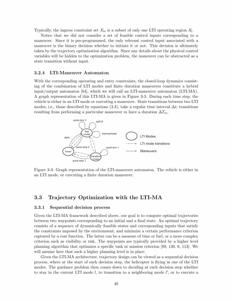
Typically, the ingress constraint set Xm is a subset of only one LTI operating region Xl.
Notice that we did not consider a set of feasible control inputs corresponding to amaneuver. Since it is pre-programmed, the only relevant control input associated with amaneuver is the binary decision whether to initiate it or not. This decision is ultimatelytaken by the trajectory optimization algorithm. Since any details about the physical controlvariables will be hidden to the optimization problem, the maneuver can be abstracted as astate transition without input.
3.2.4 LTI-Maneuver Automaton
With the corresponding operating and entry constraints, the closed-loop dynamics consist-ing of the combination of LTI modes and finite duration maneuvers constitute a hybridinput/output automaton [84], which we will call an LTI-maneuver automaton (LTI-MA).A graph representation of this LTI-MA is given in Figure 3-3. During each time step, thevehicle is either in an LTI mode or executing a maneuver. State transitions between two LTImodes, i.e., those described by equations (3.3), take a regular time interval ∆t; transitionsresulting from performing a particular maneuver m have a duration ∆Tm.
hover
fastcruise
transitioncruise
hammerhead
LTI Modes
Maneuvers
dash
quick-stop 2
LTI mode transitions
quick-turn 2split-S
quick-turn 1
quick-stop 1
Figure 3-3: Graph representation of the LTI-maneuver automaton. The vehicle is either inan LTI mode, or executing a finite duration maneuver.
3.3 Trajectory Optimization with the LTI-MA
3.3.1 Sequential decision process
Given the LTI-MA framework described above, our goal is to compute optimal trajectoriesbetween two waypoints corresponding to an initial and a final state. An optimal trajectoryconsists of a sequence of dynamically feasible states and corresponding inputs that satisfythe constraints imposed by the environment, and minimize a certain performance criterioncaptured by a cost function. The latter can be a measure of time or fuel, or a more complexcriterion such as visibility or risk. The waypoints are typically provided by a higher levelplanning algorithm that optimizes a specific task or mission criterion [89, 130, 6, 113]. Wewill assume here that such a higher planning level is in place.
Given the LTI-MA architecture, trajectory design can be viewed as a sequential decisionprocess, where at the start of each decision step, the helicopter is flying in one of the LTImodes. The guidance problem then comes down to deciding at each decision step whetherto stay in the current LTI mode l, to transition to a neighboring mode l′, or to execute a
48
certain maneuver m. However, the last option is only available if the entry conditions Xm
for that maneuver are satisfied. Furthermore, when the vehicle is in the LTI-regime, thedecision steps correspond to normal, discrete time steps. In the maneuver execution mode,on the other hand, the single decision step in which a maneuver is executed, corresponds toa number of time steps equivalent to the actual duration of the maneuver. When optimizingtime, this difference should be accounted for in the formulation of the trajectory planningproblem.
The guidance decision logic just outlined lends itself well to being formulated as a mixed-integer linear program again. The continuous optimization is now done over the states andinputs that are associated with the various LTI modes. The discrete logic and decisionsresult from partitioning the state space into the distinct LTI modes and from the option ofexecuting maneuvers when the corresponding entry conditions are satisfied. In what follows,we repeatedly apply the general MILP constraint principles (2.18) and (2.19) to derive thetrajectory planning formulation with the LTI-MA dynamics.
3.3.2 Trajectory Optimization Using MILP
Operating Region Bounds
We begin by introducing binary variables to capture the and/or logic in the convex andnonconvex constraints (3.1), (3.2), and (3.5), respectively describing the feasible state andinput sets of the LTI modes and the feasible entry states of the maneuvers. They can becaptured in the matrix form of inequality (2.19). As such, for each LTI mode l, we obtain:
x(k + 1) = Alx(k) + Blu(k)t(k + 1) = t(k) + ∆t
0 ≥ F cl x(k) + F b
l yl(k) + f l
0 ≥ Gcl u(k) + Gb
l wl(k) + gl
(3.6)
where yl(k) and wl(k) are binary vectors. The matrix F cl combines the coefficients f c
l,· and
fnl,· of the state inequalities (3.1), while matrix F b
l and vector f l encode the correspondingnonconvexities using binary logic. Similarly, matrix Gc
l combines the coefficients gcl,· and
gnl,· of the input inequalities (3.2), and matrix Gb
l and vector gl encode the associatednonconvexities.
For the maneuver entry conditions (3.5), the same principle yields:
x(k + 1) = Cmx(k) + dm
t(k + 1) = t(k) + ∆Tm
0 ≥ F cmx(k) + F b
mzm(k) + fm
(3.7)
where zm(k) is again a binary vector, F cm combines the coefficients f c
m,· and fnm,·, and F b
m
and fm encode the nonconvex structure of the entry constraints (3.5).
LTI Mode Switching
At the beginning of each decision step, the vehicle is in exactly one LTI mode l. Hence, withevery decision step k, we can associate a binary variable bl(k) that equals 1 if the vehicle isflying in mode l at the start of that decision step. Since the L modes are mutually exclusive,only one bl(k) variable out of L can be 1 at each step k. The non-active LTI modes must
49
then be “switched off”. Using principle (2.18), this can be expressed as follows:
∀l ∈ [1, . . . , L] :
x(k + 1) − Alx(k) − Blu(k) ≤ M(1 − bl(k))1−x(k + 1) + Alx(k) + Blu(k) ≤ M(1 − bl(k))1
F cl x(k) + F b
l yl(k) + f l ≤ M(1 − bl(k))1
Gcl u(k) + Gb
l wl(k) + gl ≤ M(1 − bl(k))1
(3.8a)
t(k + 1) − t(k) − ∆t ≤ 0−t(k + 1) + t(k) + ∆t ≤ 0
∑Ll=1 bl(k) = 1
(3.8b)
where 1 represents a unity vector of appropriate length. Notice that the state space equalityconstraints of the LTI mode dynamics (3.6) have been replaced by a pair of positive andnegative inequalities, such that they can be relaxed if the vehicle is not in mode l (i.e., whenbl(k) = 0). Since the time evolution equation is the same for all LTI modes, however, thecorresponding inequalities need not be relaxed.
Maneuver Execution
Similarly, we introduce a binary selection variable dm(k) for each maneuver m at eachdecision step k, which equals 1 if the maneuver is executed:
∀m ∈ [1, . . . , P ] :
x(k + 1) − Cmx(k) − dm ≤ M (1 − dm(k))1−x(k + 1) + Cmx(k) + dm ≤ M (1 − dm(k))1
F cmx(k) + F b
mzm(k) + fm ≤ M (1 − dm(k))1t(k + 1) − t(k) − ∆Tm ≤ M (1 − dm(k))
−t(k + 1) + t(k) + ∆Tm ≤ M (1 − dm(k))
(3.9a)
∑Pm=1 dm(k) ≤ 1 (3.9b)
The inequality∑P
m=1 dm(k) ≤ 1 ensures that at most one maneuver is performed at atime. This implies that if the initial conditions F c
mx(k) + F bmzm(k) + fm ≤ 0 for a certain
maneuver m are satisfied, it does not necessarily have to be executed: dm(k) can still beset to 0. However, if it is initiated, the state- and time update inequalities of the LTI modeconstraints (3.8a) and (3.8b) must be relaxed, since they are in that case determined byequations (3.4). We therefore extend constraints (3.8a) and (3.8b) as follows:
∀l ∈ [1, . . . , L] :
x(k + 1) − Alx(k) − Blu(k) ≤ M(1 − bl(k))1 + M(∑P
m=1 dm(k))1
−x(k + 1) + Alx(k) + Blu(k) ≤ M(1 − bl(k))1 + M(∑P
m=1 dm(k))1
F cl x(k) + F b
l yl(k) + f l ≤ M (1 − bl(k))1
Gcl u(k) + Gb
l wl(k) + gl ≤ M (1 − bl(k))1
(3.10a)
t(k + 1) − t(k) − ∆t ≤ M∑P
m=1 dm(k)
−t(k + 1) + t(k) + ∆t ≤ M∑P
m=1 dm(k)∑L
l=1 bl(k) = 1
(3.10b)
If no maneuver is performed, the extra relaxation term M(∑P
m=1 dm(k))1 will equal 0.Since all maneuvers start and end in one of the LTI modes, the LTI operating bounds need
50
not be relaxed by the maneuver selection variables: even if a maneuver is executed, thevehicle will still be in some LTI mode l at the start of decision step k.
3.3.3 Planning Strategies
Given the preceding LTI-MA dynamics, our next step is to compute an optimal trajectoryfrom an initial state xinit to a desired final state xf . As discussed before, these statesare typically positions with associated speeds and heading angles provided in an inertialcoordinate frame. The desired state xf will again be provided by a higher level task- ormission design algorithm that we assume is in place. Depending on the operational objectiveand the available computational resources, we can consider different planning strategies.
Fixed Horizon Planning
A first approach is to solve one (off-line) MILP problem over a fixed number of decisionsteps, with the constraint that the vehicle must have arrived within some bound of thefinal state by the end of the planning horizon. This approach requires that all relevantinformation about the mission and environment is known ahead of time, and that duringexecution of the plan, the trajectory can be accurately tracked. Introducing a planninghorizon of T decision steps and an arrival tolerance ǫ, the optimization problem has thefollowing general form:
minJfh =T−1∑
k=0
(
ℓk(x(k), u(k), b(k)) +L
∑
l=1
bl(k)ℓkl +P
∑
m=1
dm(k)ℓkm
)
(3.11a)
subject to
(3.9a), (3.9b), k = 0, . . . , T − 1(3.10a), (3.10a), k = 0, . . . , T − 1x(T ) − xf ≤ ǫ
−x(T ) + xf ≤ ǫ
x(0) = xinit
(3.11b)
Here, ℓk(x(k), u(k), b(k)) is a general (piece-wise) linear cost term associated with the kth
decision step, with b(k) some binary decision vector. ℓkl and ℓkm are constant cost factors,respectively associated with being in LTI mode l or executing maneuver m during decisionstep k. For the problem to be feasible, the horizon length T must be an upper bound onthe number of steps needed to reach the desired state.
Shortest Arrival Time
A special case of a fixed horizon planning problem is to compute the shortest time trajectorybetween the states xinit and xf . The shortest time corresponds to the minimum weightednumber of decision steps in which the final state can be reached. The weight of each stepis the actual duration of the action taken during that step. To minimize the arrival time,we can then introduce binary variables r(k) that select the step at which the final state isreached. In addition, an extra equality constraint is needed that enforces the helicopter toactually reach the desired state at one of the decision steps in the planning horizon [114].
We again consider an horizon of T decision steps and an arrival treshold ǫ. A shortest
51
time trajectory can then be computed as follows:
min Jst =T
∑
k=0
r(k)k ∆t +T−1∑
k=0
P∑
m=1
dm(k)(∆Tm − ∆t) (3.12a)
subject to
(3.9a), (3.9b), k = 0, . . . , T − 1(3.10a), (3.10a), k = 0, . . . , T − 1x(k) − xf ≤ ǫ + M(1 − r(k))1, k = 0, . . . , T
−x(k) + xf ≤ ǫ + M(1 − r(k))1, k = 0, . . . , T∑T
k=0 r(k) = 1x(0) = xinit
(3.12b)
Since only one of the r(k) binary variables equals 1, the first term in the cost function yieldsthe optimal number of decision steps needed to reach the final state, weighted by ∆t. Ifthe optimal action at the kth decision step is to stay in the LTI regime, the weight of thestep corresponds to the discretization step ∆t. However, if the optimal action is to performa maneuver (dm(k) = 1), the weight of the decision step is the maneuver duration ∆Tm.Since the first term in Jst already accounts for a weight ∆t, the latter is subtracted fromthe actual maneuver time ∆Tm.
Receding Horizon Planning
Although it is intrinsic to the motion planning problem as well, a drawback of MILP isthat the computation time increases at least polynomially with the number of variables andconstraints. Therefore, the fixed horizon approach is mainly suited for offline computation oftrajectories. For real-time applications, it can only be applied to relatively small problems,i.e., to problems with a reduced set of LTI modes and maneuvers and/or a limited numberof decision steps in which the final state can be reached. Even then, however, offlinetrajectory planning has several disadvantages. First, once the trajectory has been computed,it does not allow for changes in the vehicle dynamics or for modifications in the environmentduring execution of the plan. As such, a nominal offline planning strategy is not robustto uncertainties or disturbances. Moreover, all necessary information has to be availablebeforehand, i.e., before the vehicle starts its mission. This is often impossible and wouldexclude applications such as reconnaissance or terrain exploration. In addition, it is ourintention to use the LTI-MA framework in a real-time guidance loop, where the full rangeof the vehicle’s dynamic capabilities can be exploited in a reactive fashion.
As discussed in Chapter 2, the above limitations can be effectively addressed using areceding horizon planning strategy. The path of the vehicle is then computed iteratively andcomposed of a sequence of locally (time-)optimal segments. The length T of the planninghorizon should be chosen as a function of the available computational resources and thedistance over which the environment is fully characterized (e.g, as resulting from onboardsensor information). New information about the environment can be incorporated in theoptimization problem at each iteration, thus enabling reactive planning capabilities thatare crucial when the environment changes or is explored in real-time.
If the length of the planning horizon is relatively short and the problem complexity lowenough to solve the fixed horizon problem (3.11a)-(3.11b) or (3.12a)-(3.12b) in real-time,a first approach to a receding horizon implementation is to solve a fixed horizon problemat each time step. As the vehicle moves closer to the goal, the upper bound T on the
52
number of required decision steps can then be reduced at each iteration. If the waypointsare relatively far apart, however, and the horizon length is consequently relatively long, thismethod becomes computationally too expensive for use in real-time.
Therefore, at a certain iteration with current state xinit, we use the following, moregeneral form for the receding horizon optimization problem with the LTI-MA dynamicsover T decision steps:
minJrh =T−1∑
k=0
(
ℓk(x(k), u(k), b(k)) +L
∑
l=1
bl(k)ℓkl +P
∑
m=1
dm(k)ℓkm
)
+ ℓT (x(T ), xf , b(T ))
(3.13a)
subject to
(3.9a), (3.9b), k = 0 . . . T − 1(3.10a), (3.10a), k = 0 . . . T − 1x(0) = xinit
(3.13b)
Since the final state xf may not be reachable within T decision steps from the currentstate xinit, the arrival constraints are replaced by a terminal cost ℓT (x(T ), xf , b(T )) in theobjective function. To be applicable to the MILP framework, the terminal cost must havea piece-wise linear or piece-wise constant form. For a discussion on the role of this cost, werefer the reader back to Chapter 2.
3.4 Small-Scale Helicopter Example
We now apply the mathematical framework from Section 3.3 to a small-scale rotorcraftmodeled after MIT’s aerobatic X-Cell helicopter [142]. To keep the formulation concise,we present an approximate inertial frame model. A physically more comprehensive ap-proach using body-fixed velocities can be found in [126], in which additional binary logic isintroduced to encode the associated nonlinear kinematics.
3.4.1 Helicopter LTI Modes
Continuous-Time Version
The velocity control augmentation system of the X-Cell is described in [43] and featuresthe following command variables: body axis forward velocity ucmd and side velocity vcmd,climb rate hcmd and yaw rate rcmd. The yaw rate command is mechanized to work as aturn rate command, both at hover and forward flight. In hover, the helicopter uses tailrotor control to turn on the spot. In forward flight, lateral cyclic and tail rotor control aremixed by the control law to achieve coordinated turns, i.e., turns with zero side-slip. Thecontrol system uses gain scheduling to linearize the closed-loop dynamics around severaloperating velocities, resulting in different LTI modes. As such, the closed-loop dynamicsof the X-Cell in each LTI mode l can be accurately modeled by the following decoupled,first-order differential equations [39]:
u = − 1τul
u + 1τul
ucmd
v = − 1τvl
v + 1τvl
vcmd
h = − 1τhl
h + 1τhl
hcmd
r = − 1τrl
r + 1τrl
rcmd
(3.14)
53
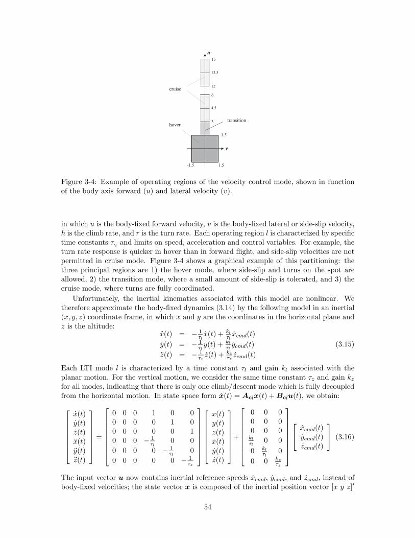
Figure 3-4: Example of operating regions of the velocity control mode, shown in functionof the body axis forward (u) and lateral velocity (v).
in which u is the body-fixed forward velocity, v is the body-fixed lateral or side-slip velocity,h is the climb rate, and r is the turn rate. Each operating region l is characterized by specifictime constants τ·l and limits on speed, acceleration and control variables. For example, theturn rate response is quicker in hover than in forward flight, and side-slip velocities are notpermitted in cruise mode. Figure 3-4 shows a graphical example of this partitioning: thethree principal regions are 1) the hover mode, where side-slip and turns on the spot areallowed, 2) the transition mode, where a small amount of side-slip is tolerated, and 3) thecruise mode, where turns are fully coordinated.
Unfortunately, the inertial kinematics associated with this model are nonlinear. Wetherefore approximate the body-fixed dynamics (3.14) by the following model in an inertial(x, y, z) coordinate frame, in which x and y are the coordinates in the horizontal plane andz is the altitude:
x(t) = − 1τl
x(t) + kl
τlxcmd(t)
y(t) = − 1τl
y(t) + kl
τlycmd(t)
z(t) = − 1τz
z(t) + kz
τzzcmd(t)
(3.15)
Each LTI mode l is characterized by a time constant τl and gain kl associated with theplanar motion. For the vertical motion, we consider the same time constant τz and gain kz
for all modes, indicating that there is only one climb/descent mode which is fully decoupledfrom the horizontal motion. In state space form x(t) = Aclx(t) + Bclu(t), we obtain:
x(t)y(t)z(t)x(t)y(t)z(t)
=
0 0 0 1 0 00 0 0 0 1 00 0 0 0 0 10 0 0 − 1
τl0 0
0 0 0 0 − 1τl
0
0 0 0 0 0 − 1τz
x(t)y(t)z(t)x(t)y(t)z(t)
+
0 0 00 0 00 0 0
kl
τl0 0
0 kl
τl0
0 0 kz
τz
xcmd(t)ycmd(t)zcmd(t)
(3.16)
The input vector u now contains inertial reference speeds xcmd, ycmd, and zcmd, instead ofbody-fixed velocities; the state vector x is composed of the inertial position vector [x y z]′
54
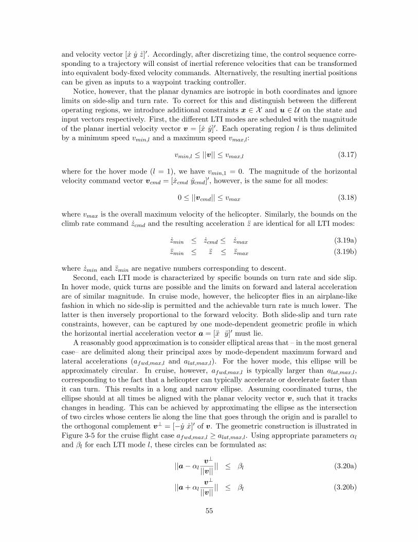
and velocity vector [x y z]′. Accordingly, after discretizing time, the control sequence corre-sponding to a trajectory will consist of inertial reference velocities that can be transformedinto equivalent body-fixed velocity commands. Alternatively, the resulting inertial positionscan be given as inputs to a waypoint tracking controller.
Notice, however, that the planar dynamics are isotropic in both coordinates and ignorelimits on side-slip and turn rate. To correct for this and distinguish between the differentoperating regions, we introduce additional constraints x ∈ X and u ∈ U on the state andinput vectors respectively. First, the different LTI modes are scheduled with the magnitudeof the planar inertial velocity vector v = [x y]′. Each operating region l is thus delimitedby a minimum speed vmin,l and a maximum speed vmax,l:
vmin,l ≤ ||v|| ≤ vmax,l (3.17)
where for the hover mode (l = 1), we have vmin,1 = 0. The magnitude of the horizontalvelocity command vector vcmd = [xcmd ycmd]
′, however, is the same for all modes:
0 ≤ ||vcmd|| ≤ vmax (3.18)
where vmax is the overall maximum velocity of the helicopter. Similarly, the bounds on theclimb rate command zcmd and the resulting acceleration z are identical for all LTI modes:
zmin ≤ zcmd ≤ zmax (3.19a)
zmin ≤ z ≤ zmax (3.19b)
where zmin and zmin are negative numbers corresponding to descent.Second, each LTI mode is characterized by specific bounds on turn rate and side slip.
In hover mode, quick turns are possible and the limits on forward and lateral accelerationare of similar magnitude. In cruise mode, however, the helicopter flies in an airplane-likefashion in which no side-slip is permitted and the achievable turn rate is much lower. Thelatter is then inversely proportional to the forward velocity. Both slide-slip and turn rateconstraints, however, can be captured by one mode-dependent geometric profile in whichthe horizontal inertial acceleration vector a = [x y]′ must lie.
A reasonably good approximation is to consider elliptical areas that – in the most generalcase– are delimited along their principal axes by mode-dependent maximum forward andlateral accelerations (afwd,max,l and alat,max,l). For the hover mode, this ellipse will beapproximately circular. In cruise, however, afwd,max,l is typically larger than alat,max,l,corresponding to the fact that a helicopter can typically accelerate or decelerate faster thanit can turn. This results in a long and narrow ellipse. Assuming coordinated turns, theellipse should at all times be aligned with the planar velocity vector v, such that it trackschanges in heading. This can be achieved by approximating the ellipse as the intersectionof two circles whose centers lie along the line that goes through the origin and is parallel tothe orthogonal complement v⊥ = [−y x]′ of v. The geometric construction is illustrated inFigure 3-5 for the cruise flight case afwd,max,l ≥ alat,max,l. Using appropriate parameters αl
and βl for each LTI mode l, these circles can be formulated as:
||a − αl
v⊥
||v|| || ≤ βl (3.20a)
||a + αl
v⊥
||v|| || ≤ βl (3.20b)
55
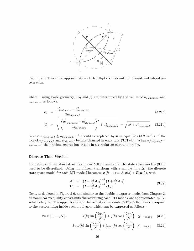
v v
afwd,max
a
T
b
-a
T
|v |
|v|__
lat,max
Figure 3-5: Two circle approximation of the elliptic constraint on forward and lateral ac-celeration.
where – using basic geometry,– αl and βl are determined by the values of afwd,max,l andalat,max,l as follows:
αl =a2
fwd,max,l − a2lat,max,l
2alat,max,l
(3.21a)
βl =
√
√
√
√
(
a2fwd,max,l − a2
lat,max,l
2alat,max,l
)2
+ a2fwd,max,l =
√
α2 + a2fwd,max,l (3.21b)
In case afwd,max,l ≤ alat,max,l, v⊥ should be replaced by v in equalities (3.20a-b) and therole of afwd,max,l and alat,max,l be interchanged in equations (3.21a-b). When afwd,max,l =alat,max,l, the previous expressions result in a circular acceleration profile.
Discrete-Time Version
To make use of the above dynamics in our MILP framework, the state space models (3.16)need to be discretized. Using the bilinear transform with a sample time ∆t, the discretestate space model for each LTI mode l becomes: x(k + 1) = Alx(k) + Blu(k), with
Al =(
I − ∆t2 Acl
)−1 (
I + ∆t2 Acl
)
Bl =(
I − ∆t2 Acl
)−1Bcl.
(3.22)
Next, as depicted in Figure 3-6, and similar to the double integrator model from Chapter 2,all nonlinear inequality constraints characterizing each LTI mode l are approximated by N -sided polygons. The upper bounds of the velocity constraints (3.17)-(3.18) then correspondto the vectors lying inside such a polygon, which can be expressed as follows:
∀n ∈ [1, . . . , N ] : x(k) sin
(
2πn
N
)
+ y(k) cos
(
2πn
N
)
≤ vmax,l (3.23)
xcmd(k) sin
(
2πn
N
)
+ ycmd(k) cos
(
2πn
N
)
≤ vmax (3.24)
56
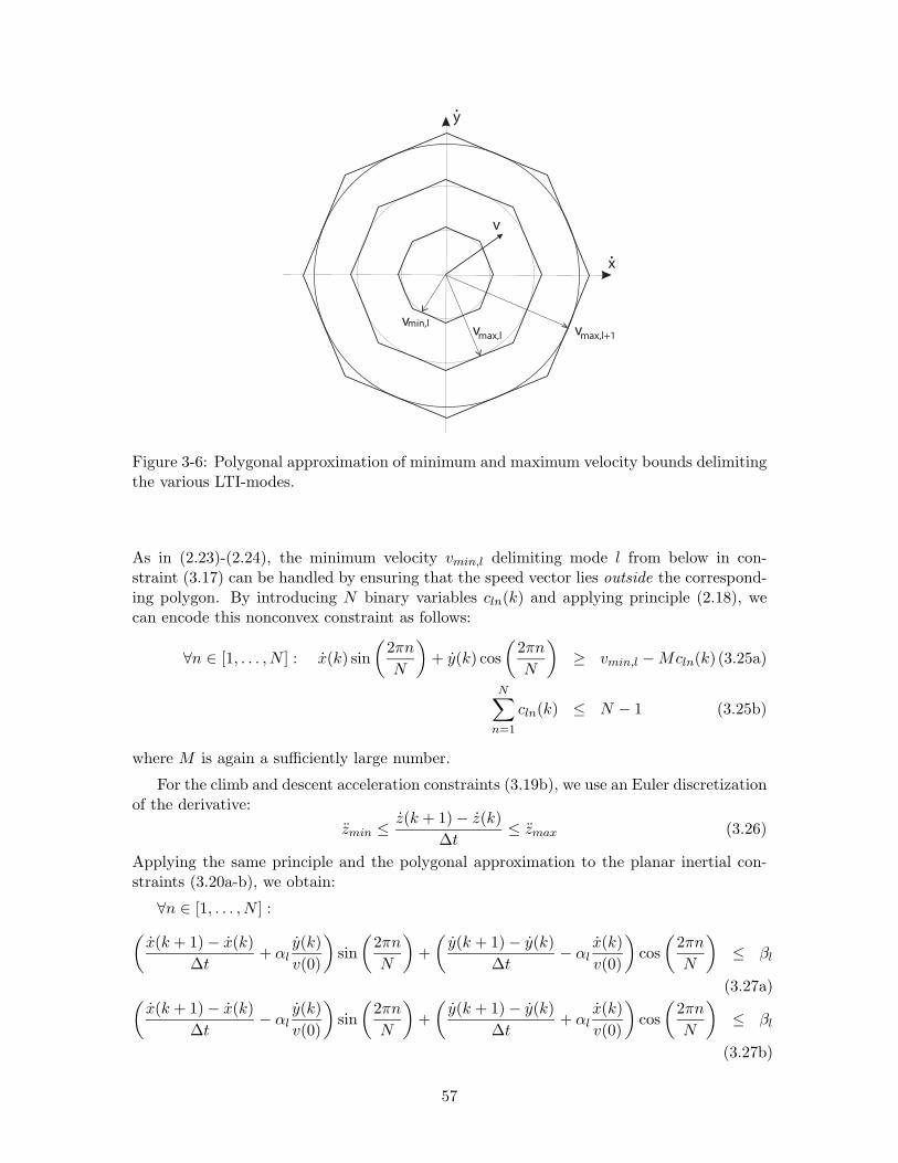
y
x
v
v vmax,l max,l+1
vmin,l
•
•
Figure 3-6: Polygonal approximation of minimum and maximum velocity bounds delimitingthe various LTI-modes.
As in (2.23)-(2.24), the minimum velocity vmin,l delimiting mode l from below in con-straint (3.17) can be handled by ensuring that the speed vector lies outside the correspond-ing polygon. By introducing N binary variables cln(k) and applying principle (2.18), wecan encode this nonconvex constraint as follows:
∀n ∈ [1, . . . , N ] : x(k) sin
(
2πn
N
)
+ y(k) cos
(
2πn
N
)
≥ vmin,l − Mcln(k) (3.25a)
N∑
n=1
cln(k) ≤ N − 1 (3.25b)
where M is again a sufficiently large number.
For the climb and descent acceleration constraints (3.19b), we use an Euler discretizationof the derivative:
zmin ≤ z(k + 1) − z(k)
∆t≤ zmax (3.26)
Applying the same principle and the polygonal approximation to the planar inertial con-straints (3.20a-b), we obtain:
∀n ∈ [1, . . . , N ] :
(
x(k + 1) − x(k)
∆t+ αl
y(k)
v(0)
)
sin
(
2πn
N
)
+
(
y(k + 1) − y(k)
∆t− αl
x(k)
v(0)
)
cos
(
2πn
N
)
≤ βl
(3.27a)(
x(k + 1) − x(k)
∆t− αl
y(k)
v(0)
)
sin
(
2πn
N
)
+
(
y(k + 1) − y(k)
∆t+ αl
x(k)
v(0)
)
cos
(
2πn
N
)
≤ βl
(3.27b)
57
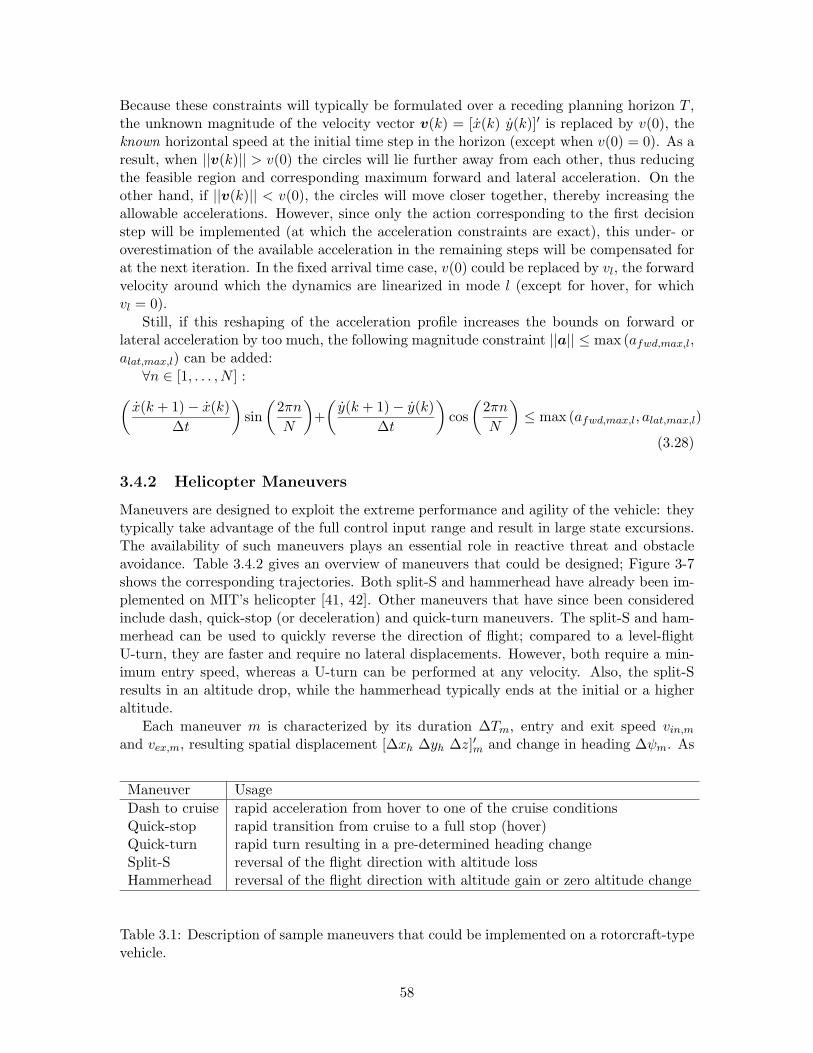
Because these constraints will typically be formulated over a receding planning horizon T ,the unknown magnitude of the velocity vector v(k) = [x(k) y(k)]′ is replaced by v(0), theknown horizontal speed at the initial time step in the horizon (except when v(0) = 0). As aresult, when ||v(k)|| > v(0) the circles will lie further away from each other, thus reducingthe feasible region and corresponding maximum forward and lateral acceleration. On theother hand, if ||v(k)|| < v(0), the circles will move closer together, thereby increasing theallowable accelerations. However, since only the action corresponding to the first decisionstep will be implemented (at which the acceleration constraints are exact), this under- oroverestimation of the available acceleration in the remaining steps will be compensated forat the next iteration. In the fixed arrival time case, v(0) could be replaced by vl, the forwardvelocity around which the dynamics are linearized in mode l (except for hover, for whichvl = 0).
Still, if this reshaping of the acceleration profile increases the bounds on forward orlateral acceleration by too much, the following magnitude constraint ||a|| ≤ max (afwd,max,l,alat,max,l) can be added:
∀n ∈ [1, . . . , N ] :
(
x(k + 1) − x(k)
∆t
)
sin
(
2πn
N
)
+
(
y(k + 1) − y(k)
∆t
)
cos
(
2πn
N
)
≤ max (afwd,max,l, alat,max,l)
(3.28)
3.4.2 Helicopter Maneuvers
Maneuvers are designed to exploit the extreme performance and agility of the vehicle: theytypically take advantage of the full control input range and result in large state excursions.The availability of such maneuvers plays an essential role in reactive threat and obstacleavoidance. Table 3.4.2 gives an overview of maneuvers that could be designed; Figure 3-7shows the corresponding trajectories. Both split-S and hammerhead have already been im-plemented on MIT’s helicopter [41, 42]. Other maneuvers that have since been consideredinclude dash, quick-stop (or deceleration) and quick-turn maneuvers. The split-S and ham-merhead can be used to quickly reverse the direction of flight; compared to a level-flightU-turn, they are faster and require no lateral displacements. However, both require a min-imum entry speed, whereas a U-turn can be performed at any velocity. Also, the split-Sresults in an altitude drop, while the hammerhead typically ends at the initial or a higheraltitude.
Each maneuver m is characterized by its duration ∆Tm, entry and exit speed vin,m
and vex,m, resulting spatial displacement [∆xh ∆yh ∆z]′m and change in heading ∆ψm. As
Maneuver Usage
Dash to cruise rapid acceleration from hover to one of the cruise conditionsQuick-stop rapid transition from cruise to a full stop (hover)Quick-turn rapid turn resulting in a pre-determined heading changeSplit-S reversal of the flight direction with altitude lossHammerhead reversal of the flight direction with altitude gain or zero altitude change
Table 3.1: Description of sample maneuvers that could be implemented on a rotorcraft-typevehicle.
58
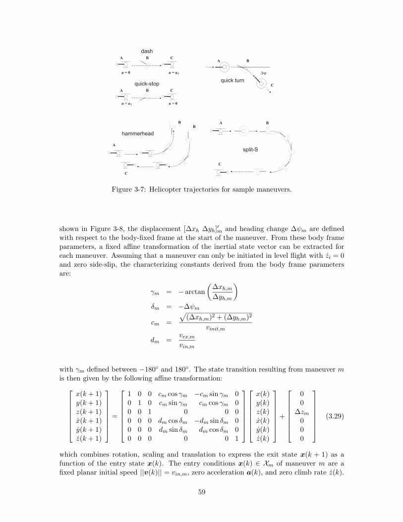
Figure 3-7: Helicopter trajectories for sample maneuvers.
shown in Figure 3-8, the displacement [∆xh ∆yh]′m and heading change ∆ψm are definedwith respect to the body-fixed frame at the start of the maneuver. From these body frameparameters, a fixed affine transformation of the inertial state vector can be extracted foreach maneuver. Assuming that a maneuver can only be initiated in level flight with zi = 0and zero side-slip, the characterizing constants derived from the body frame parametersare:
γm = − arctan
(
∆xh,m
∆yh,m
)
δm = −∆ψm
cm =
√
(∆xh,m)2 + (∆yh,m)2
vinit,m
dm =vex,m
vin,m
with γm defined between −180◦ and 180◦. The state transition resulting from maneuver mis then given by the following affine transformation:
x(k + 1)y(k + 1)z(k + 1)x(k + 1)y(k + 1)z(k + 1)
=
1 0 0 cm cos γm −cm sin γm 00 1 0 cm sin γm cm cos γm 00 0 1 0 0 00 0 0 dm cos δm −dm sin δm 00 0 0 dm sin δm dm cos δm 00 0 0 0 0 1
x(k)y(k)z(k)x(k)y(k)z(k)
+
00
∆zm
000
(3.29)
which combines rotation, scaling and translation to express the exit state x(k + 1) as afunction of the entry state x(k). The entry conditions x(k) ∈ Xm of maneuver m are afixed planar initial speed ||v(k)|| = vin,m, zero acceleration a(k), and zero climb rate z(k).
59
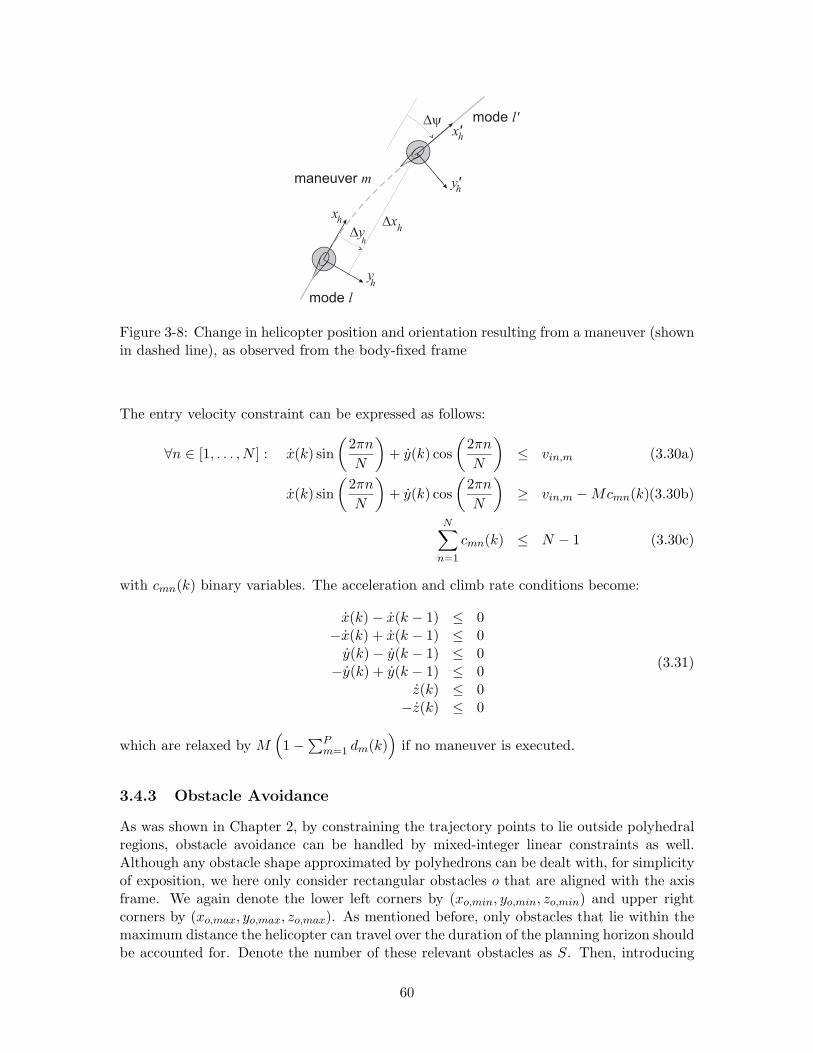
yh
y'h
xh
x'h
Dy
DyDx
mode l
maneuver m
mode l'
h
h
Figure 3-8: Change in helicopter position and orientation resulting from a maneuver (shownin dashed line), as observed from the body-fixed frame
The entry velocity constraint can be expressed as follows:
∀n ∈ [1, . . . , N ] : x(k) sin
(
2πn
N
)
+ y(k) cos
(
2πn
N
)
≤ vin,m (3.30a)
x(k) sin
(
2πn
N
)
+ y(k) cos
(
2πn
N
)
≥ vin,m − Mcmn(k)(3.30b)
N∑
n=1
cmn(k) ≤ N − 1 (3.30c)
with cmn(k) binary variables. The acceleration and climb rate conditions become:
x(k) − x(k − 1) ≤ 0−x(k) + x(k − 1) ≤ 0
y(k) − y(k − 1) ≤ 0−y(k) + y(k − 1) ≤ 0
z(k) ≤ 0−z(k) ≤ 0
(3.31)
which are relaxed by M(
1 − ∑Pm=1 dm(k)
)
if no maneuver is executed.
3.4.3 Obstacle Avoidance
As was shown in Chapter 2, by constraining the trajectory points to lie outside polyhedralregions, obstacle avoidance can be handled by mixed-integer linear constraints as well.Although any obstacle shape approximated by polyhedrons can be dealt with, for simplicityof exposition, we here only consider rectangular obstacles o that are aligned with the axisframe. We again denote the lower left corners by (xo,min, yo,min, zo,min) and upper rightcorners by (xo,max, yo,max, zo,max). As mentioned before, only obstacles that lie within themaximum distance the helicopter can travel over the duration of the planning horizon shouldbe accounted for. Denote the number of these relevant obstacles as S. Then, introducing
60
binary variables fon(k) for each time step k and each obstacle o, we repeat the avoidanceconstraints (2.30) as follows:
∀o ∈ [1, . . . , S] : x(k) ≤ xo,min + Mfo1(k)y(k) ≤ yo,min + Mfo2(k)z(k) ≤ zo,min + Mfo3(k)
−x(k) ≤ −xo,max + Mfo4(k)−y(k) ≤ −yo,max + Mfo5(k)−z(k) ≤ −zo,max + Mfo6(k)
6∑
e=1
foe(k) ≤ 5
(3.32)
Remember that these inequalities encode the requirement that each trajectory point(x(k), y(k), z(k)) must lie in at least one of the outer halfspaces defined by the faces of theS obstacles.
Again, because the trajectory consists of a discrete sequence of positions, however, thereis no guarantee that the corresponding continuous path does not intersect with the obstaclesbetween two subsequent points, e.g., during a maneuver. The obstacles must therefore beextended by a safety boundary that corresponds to the largest distance that can be traveledduring a decision step. If vmax∆t is large or when maneuvers with big displacements areconsidered, this safety envelope can be relatively large compared to the size of the obstacles,thus making the obstacle environment denser than might be acceptable. If the vehicle isin the LTI regime, the boundary can be reduced by determining intermediate trajectorypoints through linear interpolation as in expressions (2.33). For maneuver transitions,an additional avoidance check can be carried out for J sample points along the actualmaneuver trajectory. Although these points are not known a priori, they can be expressedas affine transformations of the position vector p(k) = [x(k) y(k) z(k)]′ and horizontalinertial velocity v(k) = [x(k) y(k)]′ at the start of the maneuver. Let pmj be the jth
point along the trajectory of maneuver m. Similarly to equation (3.29), by introducing amaneuver-specific constant matrix P mj and constant vector pmj for each sample point pmj ,we can write:
pmj = P mj
[
p
v
]
+ pmj (3.33)
in which [p′ v′]′ is the entry state of the maneuver. At each decision step k, the obstacleavoidance check for maneuver m and obstacle o can then be expressed as follows:
∀o ∈ [1, . . . , S], j ∈ [1, . . . , J ] : P mj
[
p(k)v(k)
]
+ pmj ≤
xo,min
yo,min
zo,min
+ M
fjo1(k)fjo2(k)fjo3(k)
−P mj
[
p(k)v(k)
]
+ pmj ≤ −
xo,max
yo,max
zo,max
+ M
fjo4(k)fjo5(k)fjo6(k)
6∑
e=1
fjoe(k) ≤ 5 (3.34)
where the same binaries are used for each maneuver m. By adding terms M(1 − dm(k)),the constraints will be relaxed if the maneuver is not executed.
61
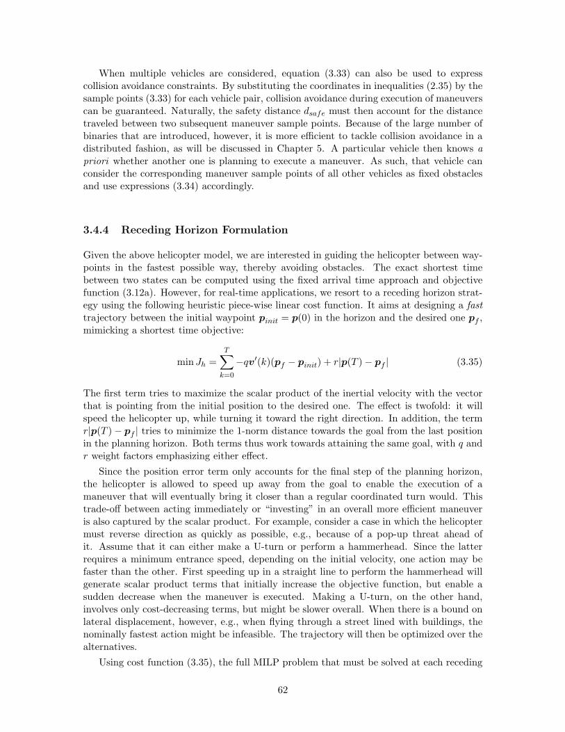
When multiple vehicles are considered, equation (3.33) can also be used to expresscollision avoidance constraints. By substituting the coordinates in inequalities (2.35) by thesample points (3.33) for each vehicle pair, collision avoidance during execution of maneuverscan be guaranteed. Naturally, the safety distance dsafe must then account for the distancetraveled between two subsequent maneuver sample points. Because of the large number ofbinaries that are introduced, however, it is more efficient to tackle collision avoidance in adistributed fashion, as will be discussed in Chapter 5. A particular vehicle then knows apriori whether another one is planning to execute a maneuver. As such, that vehicle canconsider the corresponding maneuver sample points of all other vehicles as fixed obstaclesand use expressions (3.34) accordingly.
3.4.4 Receding Horizon Formulation
Given the above helicopter model, we are interested in guiding the helicopter between way-points in the fastest possible way, thereby avoiding obstacles. The exact shortest timebetween two states can be computed using the fixed arrival time approach and objectivefunction (3.12a). However, for real-time applications, we resort to a receding horizon strat-egy using the following heuristic piece-wise linear cost function. It aims at designing a fasttrajectory between the initial waypoint pinit = p(0) in the horizon and the desired one pf ,mimicking a shortest time objective:
min Jh =T
∑
k=0
−qv′(k)(pf − pinit) + r|p(T ) − pf | (3.35)
The first term tries to maximize the scalar product of the inertial velocity with the vectorthat is pointing from the initial position to the desired one. The effect is twofold: it willspeed the helicopter up, while turning it toward the right direction. In addition, the termr|p(T ) − pf | tries to minimize the 1-norm distance towards the goal from the last positionin the planning horizon. Both terms thus work towards attaining the same goal, with q andr weight factors emphasizing either effect.
Since the position error term only accounts for the final step of the planning horizon,the helicopter is allowed to speed up away from the goal to enable the execution of amaneuver that will eventually bring it closer than a regular coordinated turn would. Thistrade-off between acting immediately or “investing” in an overall more efficient maneuveris also captured by the scalar product. For example, consider a case in which the helicoptermust reverse direction as quickly as possible, e.g., because of a pop-up threat ahead ofit. Assume that it can either make a U-turn or perform a hammerhead. Since the latterrequires a minimum entrance speed, depending on the initial velocity, one action may befaster than the other. First speeding up in a straight line to perform the hammerhead willgenerate scalar product terms that initially increase the objective function, but enable asudden decrease when the maneuver is executed. Making a U-turn, on the other hand,involves only cost-decreasing terms, but might be slower overall. When there is a bound onlateral displacement, however, e.g., when flying through a street lined with buildings, thenominally fastest action might be infeasible. The trajectory will then be optimized over thealternatives.
Using cost function (3.35), the full MILP problem that must be solved at each receding
62
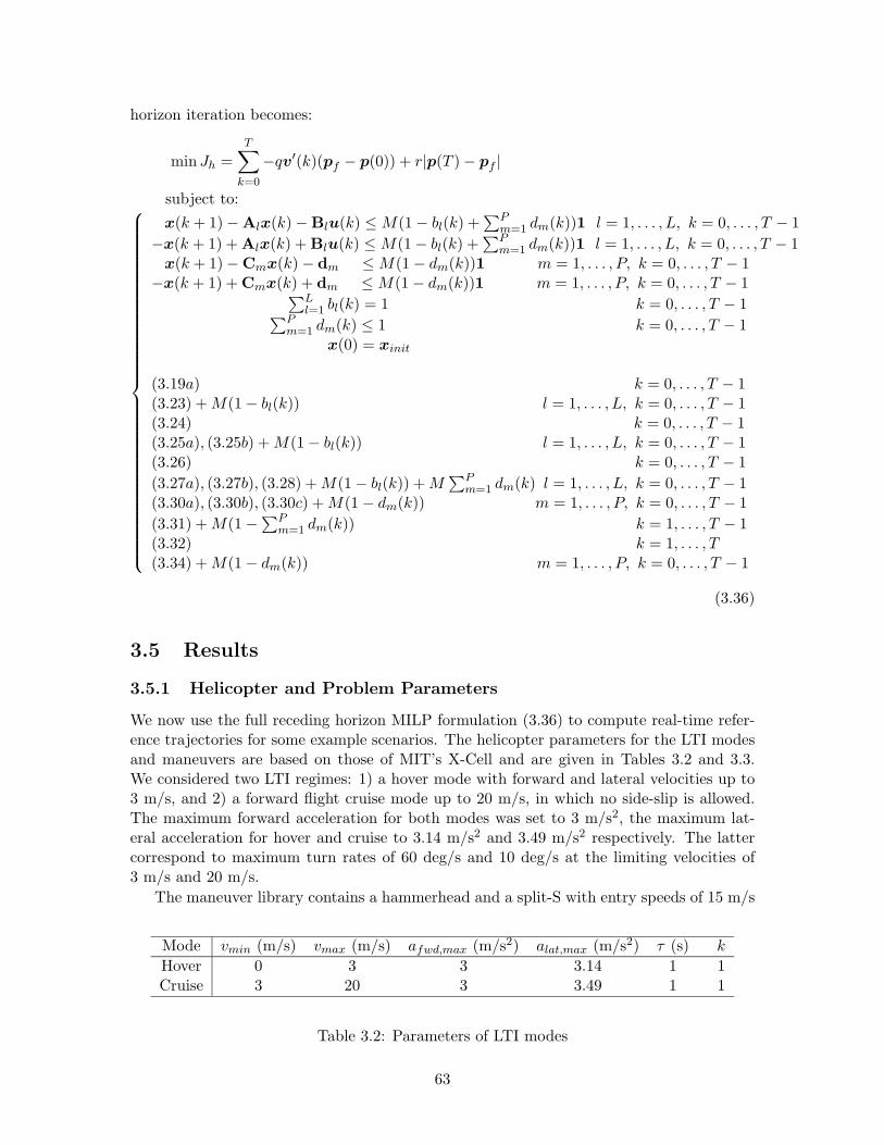
horizon iteration becomes:
minJh =
T∑
k=0
−qv′(k)(pf − p(0)) + r|p(T ) − pf |
subject to:
x(k + 1) − Alx(k) − Blu(k) ≤ M(1 − bl(k) +∑P
m=1 dm(k))1 l = 1, . . . , L, k = 0, . . . , T − 1
−x(k + 1) + Alx(k) + Blu(k) ≤ M(1 − bl(k) +∑P
m=1 dm(k))1 l = 1, . . . , L, k = 0, . . . , T − 1x(k + 1) − Cmx(k) − dm ≤ M(1 − dm(k))1 m = 1, . . . , P, k = 0, . . . , T − 1
−x(k + 1) + Cmx(k) + dm ≤ M(1 − dm(k))1 m = 1, . . . , P, k = 0, . . . , T − 1∑L
l=1 bl(k) = 1 k = 0, . . . , T − 1∑P
m=1 dm(k) ≤ 1 k = 0, . . . , T − 1x(0) = xinit
(3.19a) k = 0, . . . , T − 1(3.23) + M(1 − bl(k)) l = 1, . . . , L, k = 0, . . . , T − 1(3.24) k = 0, . . . , T − 1(3.25a), (3.25b) + M(1 − bl(k)) l = 1, . . . , L, k = 0, . . . , T − 1(3.26) k = 0, . . . , T − 1
(3.27a), (3.27b), (3.28) + M(1 − bl(k)) + M∑P
m=1 dm(k) l = 1, . . . , L, k = 0, . . . , T − 1(3.30a), (3.30b), (3.30c) + M(1 − dm(k)) m = 1, . . . , P, k = 0, . . . , T − 1
(3.31) + M(1 − ∑Pm=1 dm(k)) k = 1, . . . , T − 1
(3.32) k = 1, . . . , T(3.34) + M(1 − dm(k)) m = 1, . . . , P, k = 0, . . . , T − 1
(3.36)
3.5 Results
3.5.1 Helicopter and Problem Parameters
We now use the full receding horizon MILP formulation (3.36) to compute real-time refer-ence trajectories for some example scenarios. The helicopter parameters for the LTI modesand maneuvers are based on those of MIT’s X-Cell and are given in Tables 3.2 and 3.3.We considered two LTI regimes: 1) a hover mode with forward and lateral velocities up to3 m/s, and 2) a forward flight cruise mode up to 20 m/s, in which no side-slip is allowed.The maximum forward acceleration for both modes was set to 3 m/s2, the maximum lat-eral acceleration for hover and cruise to 3.14 m/s2 and 3.49 m/s2 respectively. The lattercorrespond to maximum turn rates of 60 deg/s and 10 deg/s at the limiting velocities of3 m/s and 20 m/s.
The maneuver library contains a hammerhead and a split-S with entry speeds of 15 m/s
Mode vmin (m/s) vmax (m/s) afwd,max (m/s2) alat,max (m/s2) τ (s) k
Hover 0 3 3 3.14 1 1Cruise 3 20 3 3.49 1 1
Table 3.2: Parameters of LTI modes
63
Maneuver ∆xh(m) ∆yh(m) ∆z (m) ∆ψ (deg) ∆T (s) vin(m/s) vex (m/s)
Split-S 6.5 10 -30 180 5 15 18Hammerhead -20 -6 0 180 7 18 18
Table 3.3: Parameters of pre-programmed maneuvers
and 18 m/s respectively. The body-fixed parameters describing them were obtained byaveraging the actual values resulting from autonomous executions of these maneuvers on theX-Cell. Notice that an ideal execution would not exhibit a lateral displacement. However,we chose to keep them because these imperfect maneuvers clearly illustrate the trade-offdecisions the MILP optimization makes in the various scenarios. In addition, we focusedon 2D trajectory planning and ignored the changes in altitude resulting from a maneuver,thus assuming that the helicopter is flying sufficiently high.
A planning horizon of T = 5 decision steps was used with ∆t = 1 s. As such, eachiteration of the planning problem had to be solved within a second. Using CPLEX 9.0 ona Pentium 4 with 2.2 GHz clock frequency, optimal or good suboptimal feasible solutionscould always be found within this hard real-time limit. The computation times ranged from0.3 s to the full 1.0 s, but were about 0.6 s on average. The settings of other parameterswere as follows: N = 16 for the polygonal approximation of circular constraints, J = 3 forthe obstacle avoidance checks between trajectory points, a 5 m safety boundary around theobstacles, and q = r = 1 for the weights in the cost function.
3.5.2 Scenarios
In each of the following scenarios, the helicopter is initially in the origin (0 m, 0 m), flyingeast at 6 m/s or 12 m/s through a corridor such as a street lined with buildings. It is thengiven the task to reverse its direction of flight and fly towards location (-100 m, 0 m) asquickly as possible. This command would typically be issued by a higher level decision unit,and could for example result from the detection of a threat ahead of the helicopter.
In the first scenario, depicted in Figure 3-9, the vehicle is flying at 12 m/s. The optimalcourse of action is to speed up to 15 m/s and execute the split-S, resulting in a quickdirection reversal with a 18 m/s exit speed. Conformable to the LTI-MA dynamics, themaneuver is considered as a discontinuous displacement, shown in dashed line. Upon exitingthe split-S, the helicopter further accelerates to its maximum speed of 20 m/s. The fullsequence to get near the waypoint at (-100 m, 0 m) takes 12 s. Solving once for the exactshortest time trajectory using strategy (3.12a)-(3.12b) yielded the same result. However,the computation took 310 s (for a T = 14 step horizon), making the approach inapplicableto online optimization.
In the second scenario, shown in Figure 3-10, the initial speed is 6 m/s. The helicopternow decides to slow down to the hover mode in which it can turn around faster. It nowtakes 6 s to make the full U-turn and 10 s total to reach the waypoint at a speed of 20 m/s.The exact time-optimal trajectory looked very similar and lasted equally long, but took471 s to compute (again using 14 decision steps as an upper bound).
Next, we considered two scenarios in which an additional obstacle was placed in theenvironment. The resulting trajectories are plotted in Figures 3-11 and 3-12, for the twostarting velocities of 12 m/s and 6 m/s respectively. Because of the restrictive bound onturn rate in the cruise mode, executing the split-S as in scenario 1 would prohibit the
64
−100 −80 −60 −40 −20 0 20 40
−50
−40
−30
−20
−10
0
10
20
30
40
50
x−East (m)
y−N
orth
(m
)
Split−S
Split−S u = 12 m/s
u = 20 m/s
Figure 3-9: Scenario 1: The helicopter is initially in (0, 0) flying at 12 m/s and needs toreverse direction towards (−100, 0) as quickly as possible. It decides to execute the split-S.
−100 −80 −60 −40 −20 0 20 40
−50
−40
−30
−20
−10
0
10
20
30
40
50
x−East (m)
y−N
orth
(m
)
U−Turn
u = 6 m/s
U−Turn
u = 20 m/s
Figure 3-10: Scenario 2: The helicopter is initially in (0, 0) flying at 6 m/s and needs toreverse direction towards (−100, 0) as quickly as possible. It decides to make a U-turn.
vehicle from safely avoiding the obstacle (which is enlarged with a 5 m safety boundary):the helicopter would be facing it with a speed of 18 m/s and insufficient distance to turnaway. The trajectory optimization therefore results in the vehicle changing heading duringthe first time step. That way it is not pointing towards the obstacle after executing thesplit-S, and has enough space to turn around it. In addition, the helicopter slows downto avoid the southern wall. In the U-turn case of Figure 3-12, the vehicle simply makes awider coordinated turn.
65
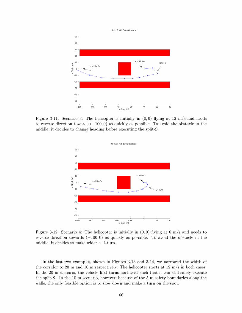
−100 −80 −60 −40 −20 0 20 40
−50
−40
−30
−20
−10
0
10
20
30
40
50
x−East (m)
y−N
orth
(m
)
Split−S with Extra Obstacle
u = 12 m/s Split−S
u = 20 m/s
Figure 3-11: Scenario 3: The helicopter is initially in (0, 0) flying at 12 m/s and needsto reverse direction towards (−100, 0) as quickly as possible. To avoid the obstacle in themiddle, it decides to change heading before executing the split-S.
−100 −80 −60 −40 −20 0 20 40
−50
−40
−30
−20
−10
0
10
20
30
40
50
x−East (m)
y−N
orth
(m
)
U−Turn with Extra Obstacle
u = 6 m/s
U−Turn
u = 20 m/s
Figure 3-12: Scenario 4: The helicopter is initially in (0, 0) flying at 6 m/s and needs toreverse direction towards (−100, 0) as quickly as possible. To avoid the obstacle in themiddle, it decides to make wider a U-turn.
In the last two examples, shown in Figures 3-13 and 3-14, we narrowed the width ofthe corridor to 20 m and 10 m respectively. The helicopter starts at 12 m/s in both cases.In the 20 m scenario, the vehicle first turns northeast such that it can still safely executethe split-S. In the 10 m scenario, however, because of the 5 m safety boundaries along thewalls, the only feasible option is to slow down and make a turn on the spot.
66
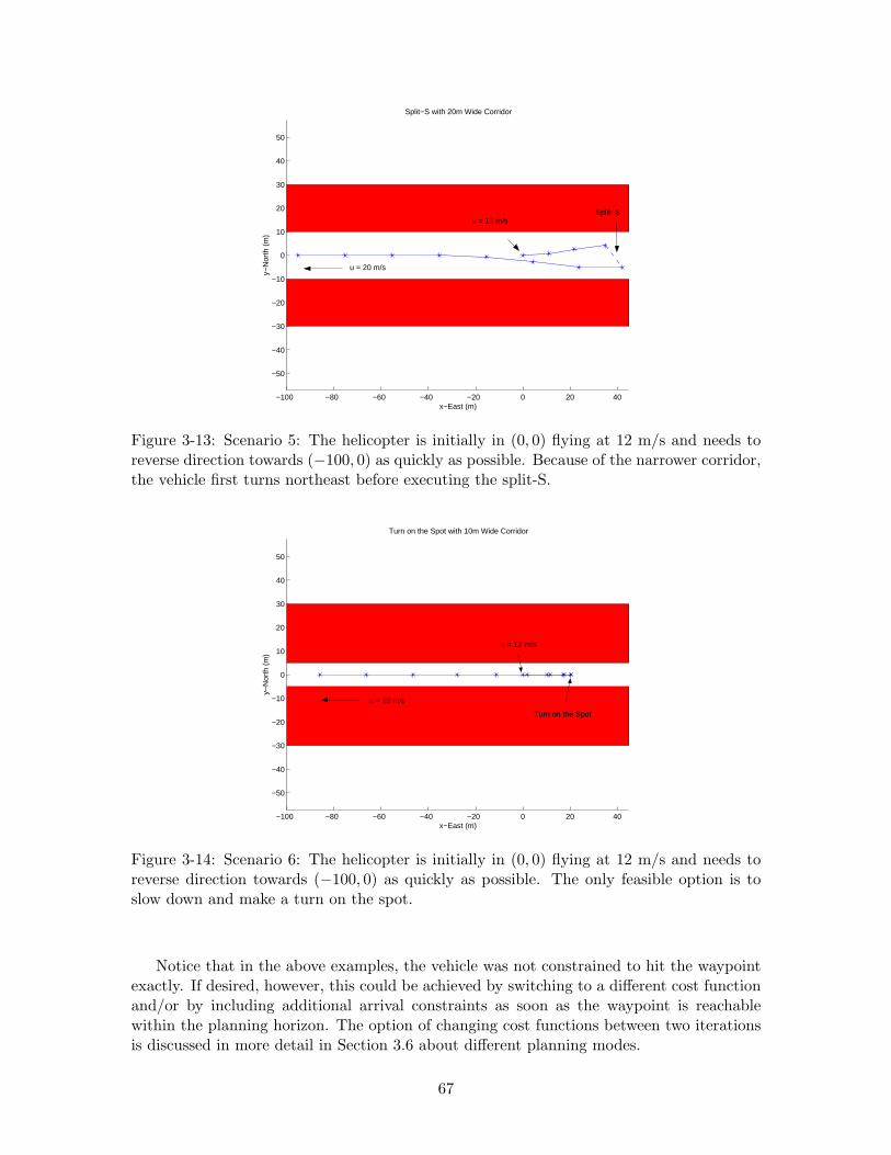
−100 −80 −60 −40 −20 0 20 40
−50
−40
−30
−20
−10
0
10
20
30
40
50
x−East (m)
y−N
orth
(m
)
Split−S with 20m Wide Corridor
u = 12 m/s
u = 20 m/s
Split−S
Figure 3-13: Scenario 5: The helicopter is initially in (0, 0) flying at 12 m/s and needs toreverse direction towards (−100, 0) as quickly as possible. Because of the narrower corridor,the vehicle first turns northeast before executing the split-S.
−100 −80 −60 −40 −20 0 20 40
−50
−40
−30
−20
−10
0
10
20
30
40
50
x−East (m)
y−N
orth
(m
)
Turn on the Spot with 10m Wide Corridor
u = 12 m/s
u = 20 m/s
Turn on the Spot
Figure 3-14: Scenario 6: The helicopter is initially in (0, 0) flying at 12 m/s and needs toreverse direction towards (−100, 0) as quickly as possible. The only feasible option is toslow down and make a turn on the spot.
Notice that in the above examples, the vehicle was not constrained to hit the waypointexactly. If desired, however, this could be achieved by switching to a different cost functionand/or by including additional arrival constraints as soon as the waypoint is reachablewithin the planning horizon. The option of changing cost functions between two iterationsis discussed in more detail in Section 3.6 about different planning modes.
67
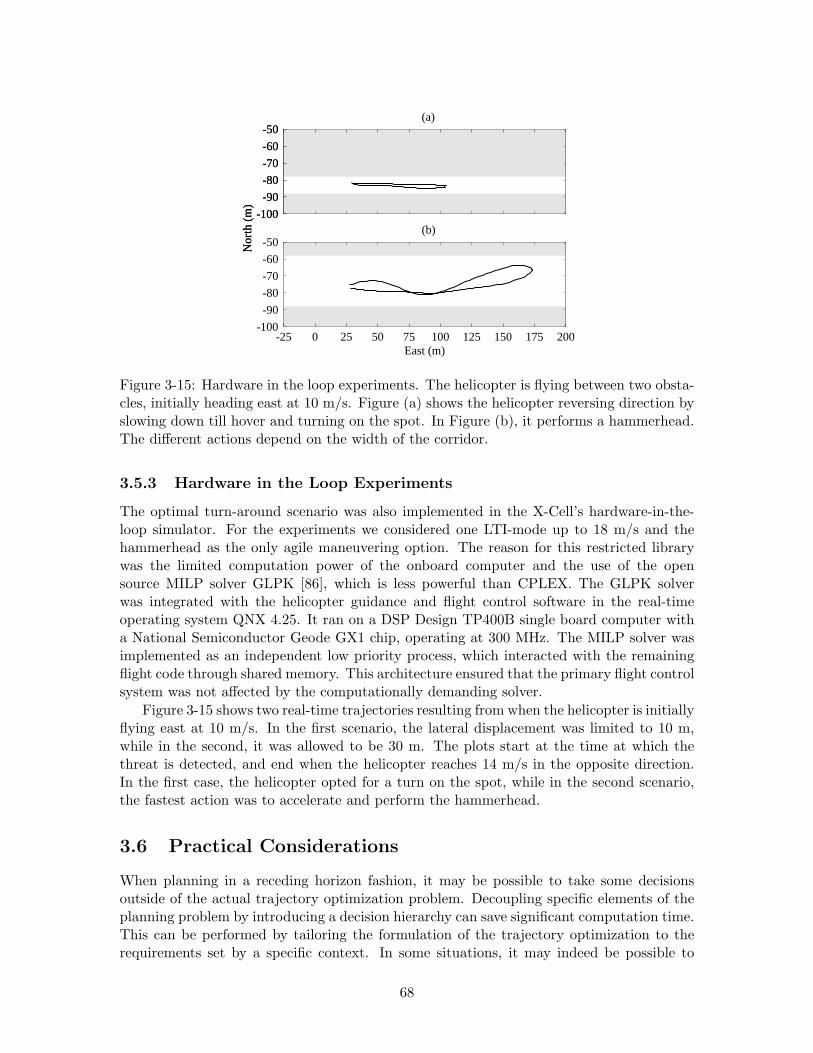
-25 0 25 50 75 100 125 150 175 200East (m)
-100
-90
-80
-70
-60
-50(b)
-100
-90
-80
-70
-60
-50
Nor
th (
m)
(a)
-100
-90
-80
-70
-60
-50
Nor
th (
m)
Figure 3-15: Hardware in the loop experiments. The helicopter is flying between two obsta-cles, initially heading east at 10 m/s. Figure (a) shows the helicopter reversing direction byslowing down till hover and turning on the spot. In Figure (b), it performs a hammerhead.The different actions depend on the width of the corridor.
3.5.3 Hardware in the Loop Experiments
The optimal turn-around scenario was also implemented in the X-Cell’s hardware-in-the-loop simulator. For the experiments we considered one LTI-mode up to 18 m/s and thehammerhead as the only agile maneuvering option. The reason for this restricted librarywas the limited computation power of the onboard computer and the use of the opensource MILP solver GLPK [86], which is less powerful than CPLEX. The GLPK solverwas integrated with the helicopter guidance and flight control software in the real-timeoperating system QNX 4.25. It ran on a DSP Design TP400B single board computer witha National Semiconductor Geode GX1 chip, operating at 300 MHz. The MILP solver wasimplemented as an independent low priority process, which interacted with the remainingflight code through shared memory. This architecture ensured that the primary flight controlsystem was not affected by the computationally demanding solver.
Figure 3-15 shows two real-time trajectories resulting from when the helicopter is initiallyflying east at 10 m/s. In the first scenario, the lateral displacement was limited to 10 m,while in the second, it was allowed to be 30 m. The plots start at the time at which thethreat is detected, and end when the helicopter reaches 14 m/s in the opposite direction.In the first case, the helicopter opted for a turn on the spot, while in the second scenario,the fastest action was to accelerate and perform the hammerhead.
3.6 Practical Considerations
When planning in a receding horizon fashion, it may be possible to take some decisionsoutside of the actual trajectory optimization problem. Decoupling specific elements of theplanning problem by introducing a decision hierarchy can save significant computation time.This can be performed by tailoring the formulation of the trajectory optimization to therequirements set by a specific context. In some situations, it may indeed be possible to
68

recognize a priori certain features of the planning problem based on the vehicle’s operatingcondition and aspects of the environment. For example, in scenario 6 from above, the split-Scould be ruled out as a feasible option and removed from the problem formulation ahead oftime. More generally, if it is possible to determine whether the vehicle state and environmentpreclude certain types of maneuvers or LTI conditions, a planning mode with a pruned set ofmaneuvers and LTI modes can be used, thus reducing the problem complexity and requiredcomputation time. Furthermore, an appropriate discretization level can be used, dependingon whether the context requires less or more precise trajectories.
These considerations are of importance in the implementation of a real-time guidancesystem. Exploiting a priori knowledge can also be used in the computation of a heuris-tic cost-to-go function. We believe that the most effective implementation will be one inwhich an online receding horizon approach is combined with an offline cost-to-go calcu-lation. Several (parameterized) cost-to-go functions could be pre-computed for different,often recurring situations, such as turning around a street corner in an urban environment.These cost-to-go functions can then be incorporated in the online optimization problem asterminal costs at the end of the planning horizon.
Such different planning modes would also allow the trajectory generation software toswitch between inertial and body-fixed frame models of the vehicle. An inertial model, forinstance, could be used to compute “high resolution” waypoints in a cluttered environment,which are then followed by solving MILP problems in a body-fixed reference frame. TheMILP optimization itself could then act as the waypoint controller.
3.7 Conclusion
This chapter presented a hybrid control architecture and model for autonomous trajectoryplanning of agile vehicles by combining multiple velocity control modes with a maneuverscheduler. The former provide the flexibility to precisely navigate between waypoints in acluttered environment, while the latter enables execution of pre-programmed maneuvers atthe limit of the vehicle capabilities. The closed-loop dynamics under this control architec-ture were described by a simple hybrid model consisting of a set of LTI modes and discrete,fixed-duration state transitions. Using this description of the dynamics, optimal trajec-tory planning through a cluttered environment was formulated as a mixed-integer linearprogram. The framework was worked out in detail for the case of a small-scale helicoptermodel based on MIT’s aerobatic X-Cell. Results for several receding horizon scenarios werepresented that illustrate the real-time applicability of the approach. In addition, somepractical considerations regarding an efficient implementation were discussed.
69

70
Chapter 4
Trajectory Planning withFeasibility and Safety Guarantees
This chapter extends the basic receding horizon trajectory problem presented in Chapter 2to account for feasibility and safety guarantees. We consider the case of a single vehiclenavigating through a cluttered environment which is only known within a certain detectionradius around the vehicle. A receding horizon strategy is presented with hard terminalconstraints that guarantee feasibility of the trajectory planning problem at all future timesteps. The trajectory computed at each iteration is constrained to end in a feasible invariantset, in which the vehicle can remain for an indefinite period of time. These invariant setsneed not be known ahead of time and are implicitly computed online. The principle isapplied to the case of a UAV with limited turn rate and minimum speed requirements, forwhich feasible invariant sets are derived in the form of loiter circles. Safety is guaranteedby further constraining the terminal feasible invariant set to contain an entry state to abacktrack pattern that brings the vehicle back to where it started. Example scenarios arepresented that illustrate the necessity of the feasibility and safety constraints when theknowledge of the environment is limited and/or hard real-time restrictions are given.
4.1 Introduction
In scenarios where the environment is not fully characterized before the mission and exploredonline, the basic trajectory planning problem presented in Chapter 2 may not always have afeasible solution. Indeed, despite the hard obstacle and collision avoidance constraints, thebasic receding horizon strategies (2.3)-(2.9) and (2.10)-(2.15) for multiple and single vehiclesrespectively have no safety guarantees regarding avoidance of obstacles and collisions in thefuture. Namely, the algorithm may fail to provide a solution in future time steps due toobstacles and other vehicles that are located beyond the planning radius of the vehicle. Forexample, the trajectory planned at the current iteration may approach an unknown obstaclethat is located just outside its detection radius or planning horizon too closely, and maynot have sufficient braking power or turn capacity to compensate for it over the next timesteps. This translates into the optimization problem becoming infeasible at a certain timestep in the future, indicating that the vehicle is on a collision course.
This chapter therefore develops additional constraints that guarantee feasibility andsafety of the receding horizon planning problem at all future iterations. The constraints areexpressed as affine transformations of the last state in the planning horizon, and, as such, are
71
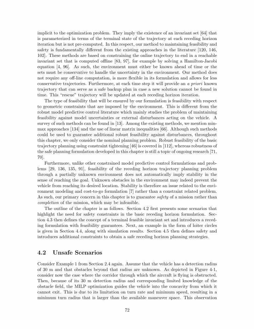
implicit to the optimization problem. They imply the existence of an invariant set [64] thatis parameterized in terms of the terminal state of the trajectory at each receding horizoniteration but is not pre-computed. In this respect, our method to maintaining feasibility andsafety is fundamentally different from the existing approaches in the literature [120, 146,102]. These methods are based on constraining the online trajectory to end in a reachableinvariant set that is computed offline [83, 97], for example by solving a Hamilton-Jacobiequation [4, 96]. As such, the environment must either be known ahead of time or thesets must be conservative to handle the uncertainty in the environment. Our method doesnot require any off-line computation, is more flexible in its formulation and allows for lessconservative trajectories. Furthermore, at each time step it will provide an a priori knowntrajectory that can serve as a safe backup plan in case a new solution cannot be found intime. This “rescue” trajectory will be updated at each receding horizon iteration.
The type of feasibility that will be ensured by our formulation is feasibility with respectto geometric constraints that are imposed by the environment. This is different from therobust model predictive control literature which mainly studies the problem of maintainingfeasibility against model uncertainties or external disturbances acting on the vehicle. Asurvey of such methods can be found in [13]. Among the existing methods, we mention min-max approaches [134] and the use of linear matrix inequalities [66]. Although such methodscould be used to guarantee additional robust feasibility against disturbances, throughoutthis chapter, we only consider the nominal planning problem. Robust feasibility of the basictrajectory planning using constraint tightening [46] is covered in [112], whereas robustness ofthe safe planning formulation developed in this chapter is still a topic of ongoing research [71,70].
Furthermore, unlike other constrained model predictive control formulations and prob-lems [29, 136, 135, 91], feasibility of the receding horizon trajectory planning problemthrough a partially unknown environment does not automatically imply stability in thesense of reaching the goal. Unknown obstacles in the environment may indeed prevent thevehicle from reaching its desired location. Stability is therefore an issue related to the envi-ronment modeling and cost-to-go formulation [7] rather than a constraint related problem.As such, our primary concern in this chapter is to guarantee safety of a mission rather thancompletion of the mission, which may be infeasible.
The outline of the chapter is as follows. Section 4.2 first presents some scenarios thathighlight the need for safety constraints in the basic receding horizon formulation. Sec-tion 4.3 then defines the concept of a terminal feasible invariant set and introduces a reced-ing formulation with feasibility guarantees. Next, an example in the form of loiter circlesis given in Section 4.4, along with simulation results. Section 4.5 then defines safety andintroduces additional constraints to obtain a safe receding horizon planning strategies.
4.2 Unsafe Scenarios
Consider Example 1 from Section 2.4 again. Assume that the vehicle has a detection radiusof 30 m and that obstacles beyond that radius are unknown. As depicted in Figure 4-1,consider now the case where the corridor through which the aircraft is flying is obstructed.Then, because of its 30 m detection radius and corresponding limited knowledge of theobstacle field, the MILP optimization guides the vehicle into the concavity from which itcannot exit. This is due to its limitation on turn rate and minimum speed, resulting in aminimum turn radius that is larger than the available maneuver space. This observation
72
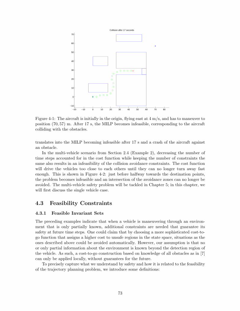
−20 −10 0 10 20 30 40 50 60 70 80
−10
0
10
20
30
40
50
60
70
Collision after 17 seconds
Figure 4-1: The aircraft is initially in the origin, flying east at 4 m/s, and has to maneuver toposition (70, 57) m. After 17 s, the MILP becomes infeasible, corresponding to the aircraftcolliding with the obstacles.
translates into the MILP becoming infeasible after 17 s and a crash of the aircraft againstan obstacle.
In the multi-vehicle scenario from Section 2.4 (Example 2), decreasing the number oftime steps accounted for in the cost function while keeping the number of constraints thesame also results in an infeasibility of the collision avoidance constraints. The cost functionwill drive the vehicles too close to each others until they can no longer turn away fastenough. This is shown in Figure 4-2: just before halfway towards the destination points,the problem becomes infeasible and an intersection of the avoidance zones can no longer beavoided. The multi-vehicle safety problem will be tackled in Chapter 5; in this chapter, wewill first discuss the single vehicle case.
4.3 Feasibility Constraints
4.3.1 Feasible Invariant Sets
The preceding examples indicate that when a vehicle is maneuvering through an environ-ment that is only partially known, additional constraints are needed that guarantee itssafety at future time steps. One could claim that by choosing a more sophisticated cost-to-go function that assigns a higher cost to unsafe regions in the state space, situations as theones described above could be avoided automatically. However, our assumption is that noor only partial information about the environment is known beyond the detection region ofthe vehicle. As such, a cost-to-go construction based on knowledge of all obstacles as in [7]can only be applied locally, without guarantees for the future.
To precisely capture what we understand by safety and how it is related to the feasibilityof the trajectory planning problem, we introduce some definitions:
73
−25 −20 −15 −10 −5 0 5 10 15 20 25
−20
−15
−10
−5
0
5
10
15
20
East (km)
Nor
th (
km)
Figure 4-2: The aircraft are initially positioned along a circle and need to fly to the oppositeside. Near the origin, the MILP becomes infeasible: the aircraft have approached each othertoo closely and an intersection of their avoidance zones cannot be avoided.
Definition 4.1 (Feasible Invariant Set): We define a feasible invariant set S(t) as astate or periodic sequence of Ip < ∞ states starting at time t that is dynamically feasible,obstacle-free, and in which the vehicle can remain for an indefinite period of time: S(t) ={x(t+ s|t) ∈ R
n, s = 0, . . . , Ip | x(t+ s|t) ∈ X (t), x(t+ s|t) /∈ O(t), x(t+ Ip|t) = x(t|t),∀s <Ip ∃u(t + s|t) ∈ U(t − 1) : x(t + s + 1|t) = Ax(t + s|t) + Bu(t + s|t)}.
Examples of such feasible invariant sets are stop states for a ground rover, hover for ahelicopter, and loiter patterns for fixed-wing UAVs that lie in a region of the environmentthat is fully characterized and will remain free of obstacles in the future. Regardless of howsuch a set is determined, it is clear that once the vehicle enters the safe invariant set, therewill always exist a dynamically feasible, obstacle-free trajectory at all future time steps.Therefore, if at each receding horizon iteration, the trajectory of the vehicle is constrainedto terminate in such a set, (nominal) feasibility at the next time step will be guaranteed.We call this set a terminal feasible invariant set:
Definition 4.2 (Terminal Feasible Invariant Set): We define a terminal feasible in-variant set S(t + T |t) as a feasible invariant set starting at the last state x(t + T |t) of thereceding horizon trajectory planning problem at time t: S(t + T |t) = {xS(t)(t + T + s|t) ∈R
n, s = 0, . . . , Ip | xS(t)(t + T |t) ≡ x(t + T |t), xS(t)(t + T + s|t) ∈ X (T ), xS(t)(t + T + s|t) /∈O(t), xS(t)(t + T + Ip|t) = xS(t)(t + T |t),∀s < Ip ∃uS(t)(t + T + s|t) ∈ U(T − 1) : xS(t)(t +T + s + 1|t) = AxS(t)(t + T + s|t) + BuS(t)(t + T + s|t)}.
Notice that the kino-dynamic constraint sets X (T ) and U(T − 1) for the terminal feasibleinvariant set are now the ones corresponding to the last state and input of the planninghorizon. The obstacle set O(t) is still the one as characterized at time t, because that iswhen the trajectory terminating in S(t + T |t) is planned.
74
4.3.2 Feasible Receding Horizon Planning Problem
Accounting for the terminal feasible invariant set in the receding horizon trajectory opti-mization yields the following extended formulation of the basic planning problem (2.10)-(2.15):
J∗T = min
T−1∑
k=0
ℓk(x(t + k|t), u(t + k|t), xf ) + fT (x(t + T |t), xf ) (4.1)
subject to:
x(t + k + 1|t) = Ax(t + k|t) + Bu(t + k|t), k = 0, . . . , T − 1 (4.2)
x(t|t) = x(t|t − 1) (4.3)
x(t + k|t) ∈ X (k) ⊇ X (k + 1), k = 1, . . . , T (4.4)
u(t + k|t) ∈ U(k) ⊇ U(k + 1), k = 0, . . . , T − 1 (4.5)
p(t + k|t) /∈ Oa(t), k = 1, . . . , T (4.6)
x(t + T |t) ∈ S(t + T |t) (4.7)
It will be referred to as PF (x(t),X (k),U(k),O(t),S(t+T |t)). Notice the additional supersetstructure X (k) ⊇ X (k + 1) and U(k) ⊇ U(k + 1) for the state and input constraint sets.Together with the terminal feasible invariant set, these additional requirements are neededto maintain a priori feasibility of the optimization problem PF (x(t + 1),X (k),U(k), O(t +1),S(t + 1 + T |t + 1)) at the next receding horizon iteration. The feasibility property isformalized in the following theorem:
Theorem 4.1: Feasibility of the trajectory optimization problem PF (x(t),X (k),U(k),O(t),S(t + T |t)) at time t implies feasibility of the problem PF (x(t + 1),X (k),U(k),O(t + 1),S(t + 1 + T |t + 1)) at time t + 1.
Proof : The proof consists of explicitly constructing a feasible solution to the next op-timization problem PF (x(t + 1),X (k),U(k),O(t + 1),S(t + 1 + T |t + 1)). Assume thata feasible solution to PF (x(t),X (k),U(k),O(t),S(t + T |t)) at time t is given by the in-put sequence u∗(t|t), u∗(t + 1|t), . . . ,u∗(t + T − 1|t) and corresponding state sequencex∗(t|t), x∗(t + 1|t), . . . ,x∗(t + T − 1|t), x∗(t + T |t), where x∗(t + T |t) ∈ S(t + T |t). Perdefinition of S(t+T |t), there exists an input u∗(t+T ) ∈ U(T −1) such that x∗(t+T +1) =Ax(t + T |t) + Bu∗(t + T ) with x∗(t + T + 1) ∈ X (T ), x∗(t + T + 1) ∈ S(t + T |t) andx∗(t + T + 1) /∈ O(t). Let a candidate solution to problem PF (·) at time t + 1 then begiven by u∗(t + 1|t + 1) = u∗(t + 1|t) ∈ U(1) ⊂ U(0), u∗(t + 2|t + 1) = u∗(t + 2|t) ∈ U(2) ⊂U(1), . . . ,u∗(t + T − 1|t + 1) = u∗(t + T − 1|t) ∈ U(T − 1) ⊂ U(T − 2), u∗(t + T |t + 1) =u∗(t + T ) ∈ U(T − 1) and x∗(t + 1|t + 1) = x∗(t + 1|t), x∗(t + 2|t + 1) = x∗(t + 2|t) ∈X (2) ⊂ X (1), . . . ,x∗(t + T |t + 1) = x∗(t + T |t) ∈ X (T ) ⊂ X (T − 1), x∗(t + 1 + T |t + 1) =x∗(t + T + 1) ∈ X (T ). The state space equations and state and input constraints arethus satisfied. Furthermore, by letting S(t + 1 + T |t + 1) = S(t + T |t), we also havex∗(t + 1 + T |t + 1) ∈ S(t + 1 + T |t + 1). Finally, because we are assuming a static envi-ronment and the new trajectory does not reach further in distance than the previous one(since it terminates in the same feasible invariant set), no new obstacles will have to be ac-counted for and the avoidance constraints are still satisfied. The candidate solution is thusfeasible which proofs the feasibility of PF (x(t + 1),X (k),U(k),O(t + 1),S(t + 1 + T |t + 1)).¤
75
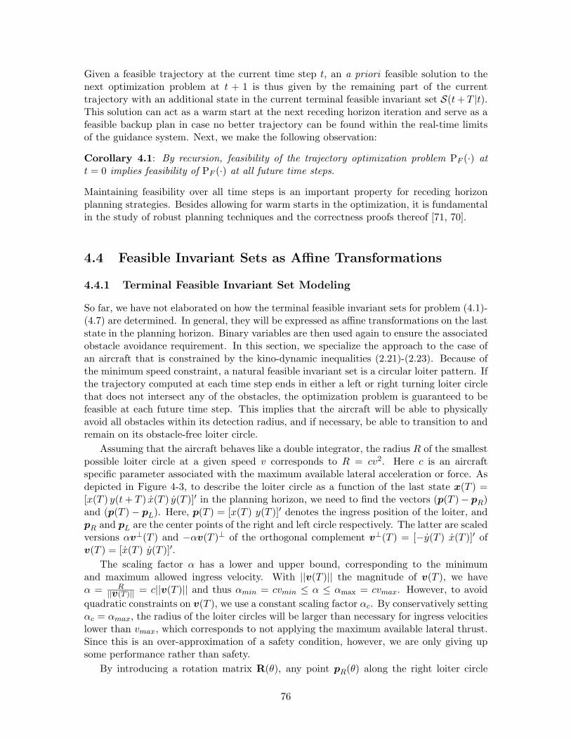
Given a feasible trajectory at the current time step t, an a priori feasible solution to thenext optimization problem at t + 1 is thus given by the remaining part of the currenttrajectory with an additional state in the current terminal feasible invariant set S(t + T |t).This solution can act as a warm start at the next receding horizon iteration and serve as afeasible backup plan in case no better trajectory can be found within the real-time limitsof the guidance system. Next, we make the following observation:
Corollary 4.1: By recursion, feasibility of the trajectory optimization problem PF (·) att = 0 implies feasibility of PF (·) at all future time steps.
Maintaining feasibility over all time steps is an important property for receding horizonplanning strategies. Besides allowing for warm starts in the optimization, it is fundamentalin the study of robust planning techniques and the correctness proofs thereof [71, 70].
4.4 Feasible Invariant Sets as Affine Transformations
4.4.1 Terminal Feasible Invariant Set Modeling
So far, we have not elaborated on how the terminal feasible invariant sets for problem (4.1)-(4.7) are determined. In general, they will be expressed as affine transformations on the laststate in the planning horizon. Binary variables are then used again to ensure the associatedobstacle avoidance requirement. In this section, we specialize the approach to the case ofan aircraft that is constrained by the kino-dynamic inequalities (2.21)-(2.23). Because ofthe minimum speed constraint, a natural feasible invariant set is a circular loiter pattern. Ifthe trajectory computed at each time step ends in either a left or right turning loiter circlethat does not intersect any of the obstacles, the optimization problem is guaranteed to befeasible at each future time step. This implies that the aircraft will be able to physicallyavoid all obstacles within its detection radius, and if necessary, be able to transition to andremain on its obstacle-free loiter circle.
Assuming that the aircraft behaves like a double integrator, the radius R of the smallestpossible loiter circle at a given speed v corresponds to R = cv2. Here c is an aircraftspecific parameter associated with the maximum available lateral acceleration or force. Asdepicted in Figure 4-3, to describe the loiter circle as a function of the last state x(T ) =[x(T ) y(t + T ) x(T ) y(T )]′ in the planning horizon, we need to find the vectors (p(T )− pR)and (p(T ) − pL). Here, p(T ) = [x(T ) y(T )]′ denotes the ingress position of the loiter, andpR and pL are the center points of the right and left circle respectively. The latter are scaledversions αv⊥(T ) and −αv(T )⊥ of the orthogonal complement v⊥(T ) = [−y(T ) x(T )]′ ofv(T ) = [x(T ) y(T )]′.
The scaling factor α has a lower and upper bound, corresponding to the minimumand maximum allowed ingress velocity. With ||v(T )|| the magnitude of v(T ), we haveα = R
||v(T )|| = c||v(T )|| and thus αmin = cvmin ≤ α ≤ αmax = cvmax. However, to avoid
quadratic constraints on v(T ), we use a constant scaling factor αc. By conservatively settingαc = αmax, the radius of the loiter circles will be larger than necessary for ingress velocitieslower than vmax, which corresponds to not applying the maximum available lateral thrust.Since this is an over-approximation of a safety condition, however, we are only giving upsome performance rather than safety.
By introducing a rotation matrix R(θ), any point pR(θ) along the right loiter circle
76

R
p
v
v
v
T
T
T
T
p
p
R
L
c
c
Figure 4-3: Safe trajectory ending in either a right or left turning loiter circle.
CR(x(T )) can then be expressed as:
pR(θ) = pR + R(θ)(αcv⊥(T ))
= (p(T ) − αcv⊥(T )) + R(θ)(αcv
⊥(T ))= p(T ) + αc(R(θ) − I)v⊥(T )
=
[
x(T )y(T )
]
+ αc
[
cos θ − 1 − sin θsin θ cos θ − 1
] [
−y(T )x(T )
]
(4.8)
Similarly, any point pL,θ along the left loiter circle CL(x(T )) is given by:
pL(θ) = pL − R(θ)(αcv⊥(T ))
= (p(T ) + αcv⊥(T )) − R(θ)(αcv
⊥(T ))= p(T ) − αc(R(θ) − I)v⊥(T )
=
[
x(T )y(T )
]
− αc
[
cos θ − 1 − sin θsin θ cos θ − 1
] [
−y(T )x(T )
]
(4.9)
4.4.2 Sampling Points Requirements
Maintaining feasibility now comes down to ensuring that either the left or right loiter circledoes not overlap with any of the obstacles that are located within the detection radius ofthe vehicle. This can be achieved by sampling both circles for fixed values of θ and byintroducing avoidance constraints similar to (2.29). To strictly follow the approach used toguarantee feasibility in the proof of Theorem 4.1, the sampling points should correspond toactual time steps ∆t, yielding N∆t = ⌈2π/(ωmax∆t)⌉ points and a sample angle of θs = 2π
N∆t.
Taking the ceiling in the expression for N∆t is required to guarantee that pL(N∆tθs) = p(T ),conformable to the definition of a terminal feasible invariant set. However, we could alsosample the loiter patterns geometrically, i.e., with a sampling angle that does not correspondto an actual time step along the circles. As long as the full circle is obstacle-free, this doesnot jeopardize the feasibility of the planning problem at the next time step. Alternativelyspeaking, the sampling comes down to a rescaling of the time step once the vehicle is in
77
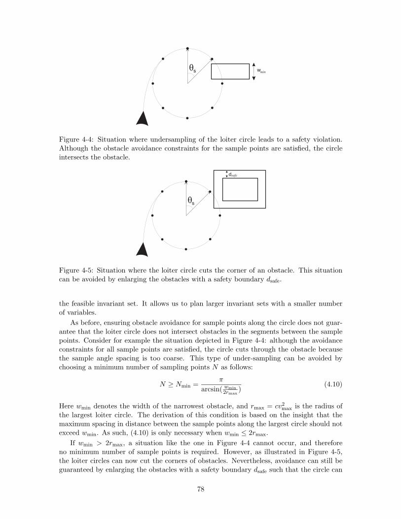
minws
Figure 4-4: Situation where undersampling of the loiter circle leads to a safety violation.Although the obstacle avoidance constraints for the sample points are satisfied, the circleintersects the obstacle.
safed
s
Figure 4-5: Situation where the loiter circle cuts the corner of an obstacle. This situationcan be avoided by enlarging the obstacles with a safety boundary dsafe.
the feasible invariant set. It allows us to plan larger invariant sets with a smaller numberof variables.
As before, ensuring obstacle avoidance for sample points along the circle does not guar-antee that the loiter circle does not intersect obstacles in the segments between the samplepoints. Consider for example the situation depicted in Figure 4-4: although the avoidanceconstraints for all sample points are satisfied, the circle cuts through the obstacle becausethe sample angle spacing is too coarse. This type of under-sampling can be avoided bychoosing a minimum number of sampling points N as follows:
N ≥ Nmin =π
arcsin( wmin
2rmax)
(4.10)
Here wmin denotes the width of the narrowest obstacle, and rmax = cv2max is the radius of
the largest loiter circle. The derivation of this condition is based on the insight that themaximum spacing in distance between the sample points along the largest circle should notexceed wmin. As such, (4.10) is only necessary when wmin ≤ 2rmax.
If wmin > 2rmax, a situation like the one in Figure 4-4 cannot occur, and thereforeno minimum number of sample points is required. However, as illustrated in Figure 4-5,the loiter circles can now cut the corners of obstacles. Nevertheless, avoidance can still beguaranteed by enlarging the obstacles with a safety boundary dsafe such that the circle can
78
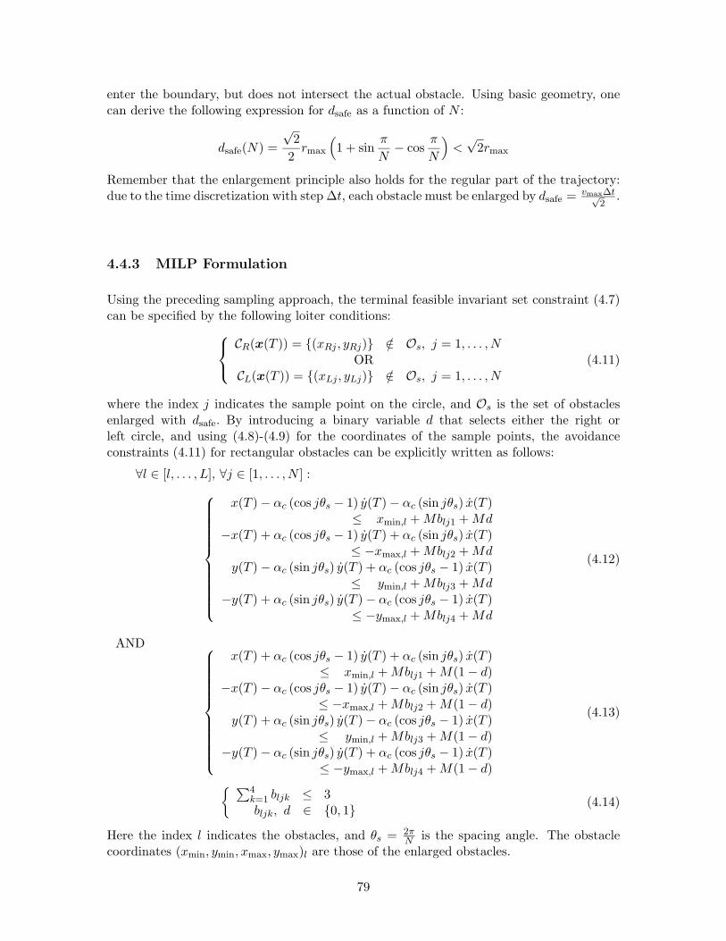
enter the boundary, but does not intersect the actual obstacle. Using basic geometry, onecan derive the following expression for dsafe as a function of N :
dsafe(N) =
√2
2rmax
(
1 + sinπ
N− cos
π
N
)
<√
2rmax
Remember that the enlargement principle also holds for the regular part of the trajectory:due to the time discretization with step ∆t, each obstacle must be enlarged by dsafe = vmax∆t√
2.
4.4.3 MILP Formulation
Using the preceding sampling approach, the terminal feasible invariant set constraint (4.7)can be specified by the following loiter conditions:
CR(x(T )) = {(xRj , yRj)} /∈ Os, j = 1, . . . , NOR
CL(x(T )) = {(xLj , yLj)} /∈ Os, j = 1, . . . , N(4.11)
where the index j indicates the sample point on the circle, and Os is the set of obstaclesenlarged with dsafe. By introducing a binary variable d that selects either the right orleft circle, and using (4.8)-(4.9) for the coordinates of the sample points, the avoidanceconstraints (4.11) for rectangular obstacles can be explicitly written as follows:
∀l ∈ [l, . . . , L], ∀j ∈ [1, . . . , N ] :
x(T ) − αc (cos jθs − 1) y(T ) − αc (sin jθs) x(T )≤ xmin,l + Mblj1 + Md
−x(T ) + αc (cos jθs − 1) y(T ) + αc (sin jθs) x(T )≤ −xmax,l + Mblj2 + Md
y(T ) − αc (sin jθs) y(T ) + αc (cos jθs − 1) x(T )≤ ymin,l + Mblj3 + Md
−y(T ) + αc (sin jθs) y(T ) − αc (cos jθs − 1) x(T )≤ −ymax,l + Mblj4 + Md
(4.12)
AND
x(T ) + αc (cos jθs − 1) y(T ) + αc (sin jθs) x(T )≤ xmin,l + Mblj1 + M(1 − d)
−x(T ) − αc (cos jθs − 1) y(T ) − αc (sin jθs) x(T )≤ −xmax,l + Mblj2 + M(1 − d)
y(T ) + αc (sin jθs) y(T ) − αc (cos jθs − 1) x(T )≤ ymin,l + Mblj3 + M(1 − d)
−y(T ) − αc (sin jθs) y(T ) + αc (cos jθs − 1) x(T )≤ −ymax,l + Mblj4 + M(1 − d)
(4.13)
{∑4
k=1 bljk ≤ 3bljk, d ∈ {0, 1} (4.14)
Here the index l indicates the obstacles, and θs = 2πN
is the spacing angle. The obstaclecoordinates (xmin, ymin, xmax, ymax)l are those of the enlarged obstacles.
79
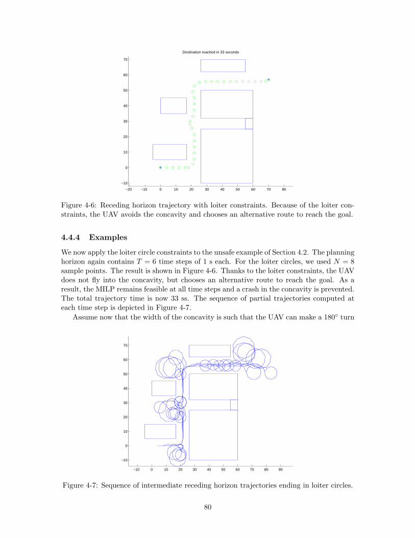
−20 −10 0 10 20 30 40 50 60 70 80
−10
0
10
20
30
40
50
60
70
Destination reached in 33 seconds
Figure 4-6: Receding horizon trajectory with loiter constraints. Because of the loiter con-straints, the UAV avoids the concavity and chooses an alternative route to reach the goal.
4.4.4 Examples
We now apply the loiter circle constraints to the unsafe example of Section 4.2. The planninghorizon again contains T = 6 time steps of 1 s each. For the loiter circles, we used N = 8sample points. The result is shown in Figure 4-6. Thanks to the loiter constraints, the UAVdoes not fly into the concavity, but chooses an alternative route to reach the goal. As aresult, the MILP remains feasible at all time steps and a crash in the concavity is prevented.The total trajectory time is now 33 ss. The sequence of partial trajectories computed ateach time step is depicted in Figure 4-7.
Assume now that the width of the concavity is such that the UAV can make a 180◦ turn
−10 0 10 20 30 40 50 60 70 80 90
−10
0
10
20
30
40
50
60
70
Figure 4-7: Sequence of intermediate receding horizon trajectories ending in loiter circles.
80
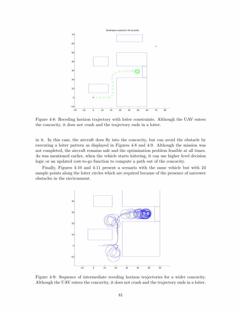
−20 −10 0 10 20 30 40 50 60 70 80
−10
0
10
20
30
40
50
60
70
Destination reached in 40 seconds
Figure 4-8: Receding horizon trajectory with loiter constraints. Although the UAV entersthe concavity, it does not crash and the trajectory ends in a loiter.
in it. In this case, the aircraft does fly into the concavity, but can avoid the obstacle byexecuting a loiter pattern as displayed in Figures 4-8 and 4-9. Although the mission wasnot completed, the aircraft remains safe and the optimization problem feasible at all times.As was mentioned earlier, when the vehicle starts loitering, it can use higher level decisionlogic or an updated cost-to-go function to compute a path out of the concavity.
Finally, Figures 4-10 and 4-11 present a scenario with the same vehicle but with 24sample points along the loiter circles which are required because of the presence of narrowerobstacles in the environment.
−10 0 10 20 30 40 50 60
−10
0
10
20
30
40
Figure 4-9: Sequence of intermediate receding horizon trajectories for a wider concavity.Although the UAV enters the concavity, it does not crash and the trajectory ends in a loiter.
81
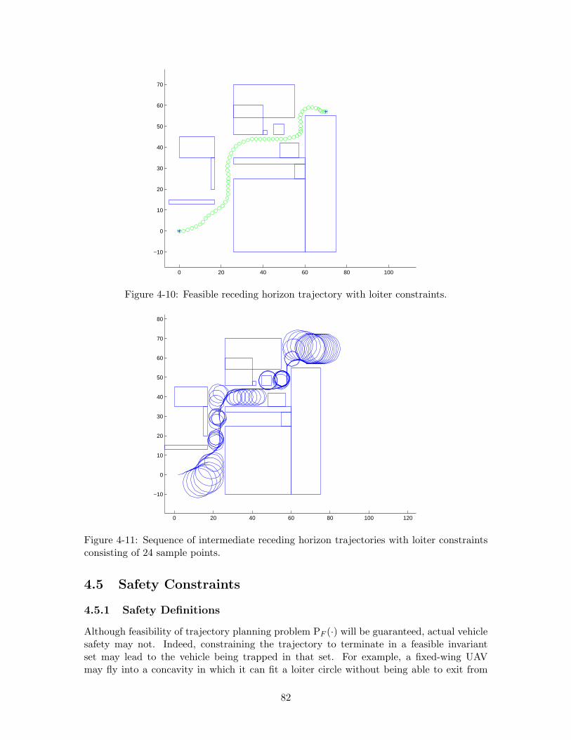
0 20 40 60 80 100
−10
0
10
20
30
40
50
60
70
Figure 4-10: Feasible receding horizon trajectory with loiter constraints.
0 20 40 60 80 100 120
−10
0
10
20
30
40
50
60
70
80
Figure 4-11: Sequence of intermediate receding horizon trajectories with loiter constraintsconsisting of 24 sample points.
4.5 Safety Constraints
4.5.1 Safety Definitions
Although feasibility of trajectory planning problem PF (·) will be guaranteed, actual vehiclesafety may not. Indeed, constraining the trajectory to terminate in a feasible invariantset may lead to the vehicle being trapped in that set. For example, a fixed-wing UAVmay fly into a concavity in which it can fit a loiter circle without being able to exit from
82
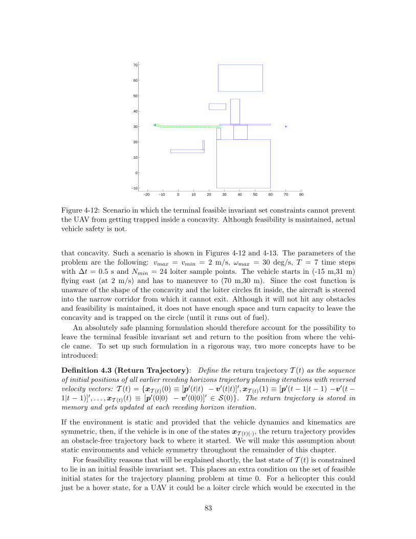
−20 −10 0 10 20 30 40 50 60 70 80
−10
0
10
20
30
40
50
60
70
Figure 4-12: Scenario in which the terminal feasible invariant set constraints cannot preventthe UAV from getting trapped inside a concavity. Although feasibility is maintained, actualvehicle safety is not.
that concavity. Such a scenario is shown in Figures 4-12 and 4-13. The parameters of theproblem are the following: vmax = vmin = 2 m/s, ωmax = 30 deg/s, T = 7 time stepswith ∆t = 0.5 s and Nmin = 24 loiter sample points. The vehicle starts in (-15 m,31 m)flying east (at 2 m/s) and has to maneuver to (70 m,30 m). Since the cost function isunaware of the shape of the concavity and the loiter circles fit inside, the aircraft is steeredinto the narrow corridor from which it cannot exit. Although it will not hit any obstaclesand feasibility is maintained, it does not have enough space and turn capacity to leave theconcavity and is trapped on the circle (until it runs out of fuel).
An absolutely safe planning formulation should therefore account for the possibility toleave the terminal feasible invariant set and return to the position from where the vehi-cle came. To set up such formulation in a rigorous way, two more concepts have to beintroduced:
Definition 4.3 (Return Trajectory): Define the return trajectory T (t) as the sequenceof initial positions of all earlier receding horizons trajectory planning iterations with reversedvelocity vectors: T (t) = {xT (t)(0) ≡ [p′(t|t) − v′(t|t)]′, xT (t)(1) ≡ [p′(t − 1|t − 1) −v′(t −1|t − 1)]′, . . . ,xT (t)(t) ≡ [p′(0|0) − v′(0|0)]′ ∈ S(0)}. The return trajectory is stored inmemory and gets updated at each receding horizon iteration.
If the environment is static and provided that the vehicle dynamics and kinematics aresymmetric, then, if the vehicle is in one of the states xT (t)(·), the return trajectory providesan obstacle-free trajectory back to where it started. We will make this assumption aboutstatic environments and vehicle symmetry throughout the remainder of this chapter.
For feasibility reasons that will be explained shortly, the last state of T (t) is constrainedto lie in an initial feasible invariant set. This places an extra condition on the set of feasibleinitial states for the trajectory planning problem at time 0. For a helicopter this couldjust be a hover state, for a UAV it could be a loiter circle which would be executed in the
83
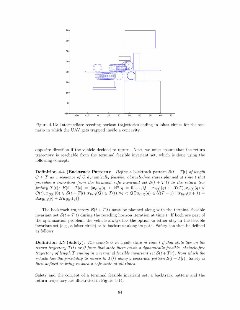
−20 −10 0 10 20 30 40 50 60 70−10
0
10
20
30
40
50
60
70
Figure 4-13: Intermediate receding horizon trajectories ending in loiter circles for the sce-nario in which the UAV gets trapped inside a concavity.
opposite direction if the vehicle decided to return. Next, we must ensure that the returntrajectory is reachable from the terminal feasible invariant set, which is done using thefollowing concept:
Definition 4.4 (Backtrack Pattern): Define a backtrack pattern B(t + T |t) of lengthQ ≤ T as a sequence of Q dynamically feasible, obstacle-free states planned at time t thatprovides a transition from the terminal safe invariant set S(t + T |t) to the return tra-jectory T (t): B(t + T |t) = {xB(t)(q) ∈ R
n, q = 0, . . . , Q | xB(t)(q) ∈ X (T ), xB(t)(q) /∈O(t), xB(t)(0) ∈ S(t + T |t), xB(t)(Q) ∈ T (t),∀q < Q∃uB(t)(q) ∈ U(T − 1) : xB(t)(q + 1) =AxB(t)(q) + BuB(t)(q)}.
The backtrack trajectory B(t + T |t) must be planned along with the terminal feasibleinvariant set S(t + T |t) during the receding horizon iteration at time t. If both are part ofthe optimization problem, the vehicle always has the option to either stay in the feasibleinvariant set (e.g., a loiter circle) or to backtrack along its path. Safety can then be definedas follows:
Definition 4.5 (Safety): The vehicle is in a safe state at time t if that state lies on thereturn trajectory T (t) or if from that state there exists a dynamically feasible, obstacle-freetrajectory of length T ending in a terminal feasible invariant set S(t + T |t), from which thevehicle has the possibility to return to T (t) along a backtrack pattern B(t + T |t). Safety isthen defined as being in such a safe state at all times.
Safety and the concept of a terminal feasible invariant set, a backtrack pattern and thereturn trajectory are illustrated in Figure 4-14.
84

Figure 4-14: Safe receding horizon trajectory of T time steps ending in a terminal feasibleinvariant set S(t+T |t) and with backtrack pattern B(t+T |t) to the return trajectory T (t).
4.5.2 Safe Feasible Receding Horizon Planning Problem
Using the concepts defined above, we can now extend the feasible receding horizon trajectoryplanning problem (4.1)-(4.7) to account for safety. Consider the following formulation:
J∗T = min
T−1∑
k=0
ℓk(x(t + k|t), u(t + k|t), xf ) + fT (x(t + T |t), xf ) (4.15)
subject to:
x(t + k + 1|t) = Ax(t + k|t) + Bu(t + k|t),k = 0, . . . , T − 1 (4.16)
x(t|t) = x(t|t − 1) (4.17)
x(t + k|t) ∈ X (k) ⊇ X (k + 1),
k = 1, . . . , T (4.18)
u(t + k|t) ∈ U(k) ⊇ U(k + 1),
k = 0, . . . , T − 1 (4.19)
p(t + k|t) /∈ Oa(t), k = 1, . . . , T (4.20)
AND{
x(t + T |t)∃s ∈ {0, . . . , Ip − 1} : xS(t)(t + T + s|t)
∈∈
S(t + T |t)B(t + T |t) (4.21)
OR
{x(t + T |t) ∈ T (t) (4.22)
where Ip is the period of the terminal feasible invariant set S(t + T |t) of interest. Con-straints (4.21) express that the vehicle must have the option to leave S(t + T |t) andtransition to the backtrack pattern B(t + T |t) to eventually arrive on the return tra-jectory T (t). Either the combination of the two constraints (4.21) ‘OR’ the single con-straint (4.22) must be satisfied to guarantee safety of the vehicle at all future time steps.Constraint (4.22) is necessary to maintain feasibility of the problem when the vehicle isalready on the return trajectory. Since it may not be able to fit terminal feasible invariantsets in the environment when it is returning, the return trajectory then still provides thevehicle with a feasible solution. We denote the above trajectory optimization problem byPS(x(t),X (k),U(k),O(t),S(t + T |t),B(t + T |t), T (t)).
85
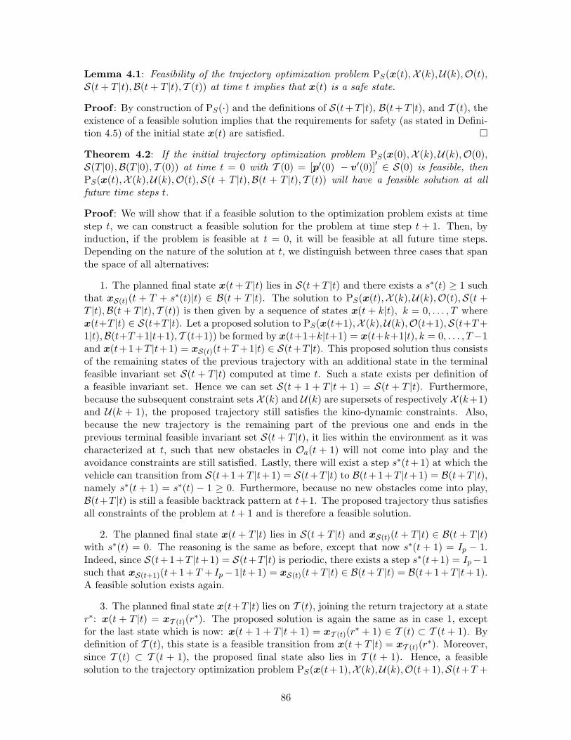
Lemma 4.1: Feasibility of the trajectory optimization problem PS(x(t),X (k),U(k),O(t),S(t + T |t),B(t + T |t), T (t)) at time t implies that x(t) is a safe state.
Proof : By construction of PS(·) and the definitions of S(t+T |t), B(t+T |t), and T (t), theexistence of a feasible solution implies that the requirements for safety (as stated in Defini-tion 4.5) of the initial state x(t) are satisfied. ¤
Theorem 4.2: If the initial trajectory optimization problem PS(x(0),X (k),U(k),O(0),S(T |0),B(T |0), T (0)) at time t = 0 with T (0) = [p′(0) − v′(0)]′ ∈ S(0) is feasible, thenPS(x(t),X (k),U(k),O(t),S(t + T |t),B(t + T |t), T (t)) will have a feasible solution at allfuture time steps t.
Proof : We will show that if a feasible solution to the optimization problem exists at timestep t, we can construct a feasible solution for the problem at time step t + 1. Then, byinduction, if the problem is feasible at t = 0, it will be feasible at all future time steps.Depending on the nature of the solution at t, we distinguish between three cases that spanthe space of all alternatives:
1. The planned final state x(t + T |t) lies in S(t + T |t) and there exists a s∗(t) ≥ 1 suchthat xS(t)(t + T + s∗(t)|t) ∈ B(t + T |t). The solution to PS(x(t),X (k),U(k),O(t),S(t +T |t),B(t + T |t), T (t)) is then given by a sequence of states x(t + k|t), k = 0, . . . , T wherex(t+T |t) ∈ S(t+T |t). Let a proposed solution to PS(x(t+1),X (k),U(k),O(t+1),S(t+T +1|t),B(t+T +1|t+1), T (t+1)) be formed by x(t+1+k|t+1) = x(t+k+1|t), k = 0, . . . , T−1and x(t+1+T |t+1) = xS(t)(t+T +1|t) ∈ S(t+T |t). This proposed solution thus consistsof the remaining states of the previous trajectory with an additional state in the terminalfeasible invariant set S(t + T |t) computed at time t. Such a state exists per definition ofa feasible invariant set. Hence we can set S(t + 1 + T |t + 1) = S(t + T |t). Furthermore,because the subsequent constraint sets X (k) and U(k) are supersets of respectively X (k+1)and U(k + 1), the proposed trajectory still satisfies the kino-dynamic constraints. Also,because the new trajectory is the remaining part of the previous one and ends in theprevious terminal feasible invariant set S(t + T |t), it lies within the environment as it wascharacterized at t, such that new obstacles in Oa(t + 1) will not come into play and theavoidance constraints are still satisfied. Lastly, there will exist a step s∗(t+1) at which thevehicle can transition from S(t+1+T |t+1) = S(t+T |t) to B(t+1+T |t+1) = B(t+T |t),namely s∗(t + 1) = s∗(t) − 1 ≥ 0. Furthermore, because no new obstacles come into play,B(t+T |t) is still a feasible backtrack pattern at t+1. The proposed trajectory thus satisfiesall constraints of the problem at t + 1 and is therefore a feasible solution.
2. The planned final state x(t + T |t) lies in S(t + T |t) and xS(t)(t + T |t) ∈ B(t + T |t)with s∗(t) = 0. The reasoning is the same as before, except that now s∗(t + 1) = Ip − 1.Indeed, since S(t+1+T |t+1) = S(t+T |t) is periodic, there exists a step s∗(t+1) = Ip−1such that xS(t+1)(t+1+T + Ip − 1|t+1) = xS(t)(t+T |t) ∈ B(t+T |t) = B(t+1+T |t+1).A feasible solution exists again.
3. The planned final state x(t+T |t) lies on T (t), joining the return trajectory at a stater∗: x(t + T |t) = xT (t)(r
∗). The proposed solution is again the same as in case 1, exceptfor the last state which is now: x(t + 1 + T |t + 1) = xT (t)(r
∗ + 1) ∈ T (t) ⊂ T (t + 1). Bydefinition of T (t), this state is a feasible transition from x(t + T |t) = xT (t)(r
∗). Moreover,since T (t) ⊂ T (t + 1), the proposed final state also lies in T (t + 1). Hence, a feasiblesolution to the trajectory optimization problem PS(x(t+1),X (k),U(k),O(t+1),S(t+T +
86
1|t),B(t + T + 1|t + 1), T (t + 1)) exists in this case as well. ¤
Corollary 4.2: By Lemma 4.1 and Theorem 4.1, if a feasible solution to the initial trajec-tory optimization problem PS(x(0),X (k),U(k),O(0), S(T |0),B(T |0), T (0)) at time t = 0exists, safety will be maintained at all times.
Remarks
1. Notice that the theorem does not provide performance or stability guarantees in thesense of reaching the goal. We are indeed mainly interested in a problem formulation thatprovides feasibility and safety guarantees as a basis before tackling stability. As discussed inthe introduction, the latter is primarily related to the cost-to-go function. The optimizationproblem might indeed keep the vehicle trapped in a local minimum corresponding to stayingin the safe invariant set. Furthermore, since at the start of a mission, the environment isnot characterized beyond a certain distance and new obstacles are detected as the vehiclemaneuvers through the environment, the vehicle may only realize along the way that thegoal might actually not be reachable. In both cases, a higher level decision making algorithmcan then decide to let the vehicle transition to its backtrack pattern and return trajectory orto incorporate new information about destination and obstacles in the cost function. Thiscould simply consist of a change of pf to p(0), i.e., the position where the vehicle started.The constraints of the optimization will remain the same, however. Regardless of the actualcost function, a safe trajectory back to the starting point will always exist.
2. The fact that a feasible solution is known a priori can be exploited when an optimal orfeasible solution cannot be found within the timing constraints of real-time guidance system.The vehicle can then resort to the a priori solution as a safe backup plan. Moreover, the apriori solution can be used as a warm start for the optimization routine.
3. We assumed that the environment is static, such that the parts of the environmentthat were characterized when the vehicle maneuvered through it do not change. Thisassumption was needed to maintain an obstacle-free return trajectory T (t). However, ifthe environment is dynamic beyond the current detection region, the vehicle still has theterminal feasible invariant set S(t + T |t) to resort to. More generally, if the constraints∃s ∈ {0, . . . , Smax} : xS(t)(t + T + s|t) ∈ B(t + T |t) and x(t + T |t) ∈ T (t) are removed, weget the original formulation from Section 4.3 again, for which feasibility can still be proved:the vehicle can always remain in S(t + T |t). However, safety according to Definition 4.5does not necessarily hold then: as shown in the scenario of Figure 4-12, the vehicle mayget trapped in S(t + T |t). If we are only interested in maintaining feasibility through apartially-known environment, however, problem formulation (4.1)-(4.7) suffices. We willcall this “minimal safety” and use it for the distributed algorithm in Chapter 5.
4. In practice, the OR-constraint in the optimization could be decided upon by a higherlevel planning unit before the next actual receding horizon iteration. Indeed, in case thevehicle is on its way back, the terminal safe invariant set and backtrack pattern constraintsare not strictly necessary: the vehicle knows it has a safe way back to its starting point. Onthe other hand, when still moving towards the goal point, the vehicle should be able to fitits terminal feasible invariant sets in the environment. In that case, the x(t + T |t) ∈ T (t)constraint can be removed. Again, the vehicle already knows that it could fly backwardsalong a feasible backtrack pattern. The return trajectory constraint is only needed tomaintain feasibility of the same problem formulation in case the vehicle cannot fit terminalfeasible invariant sets in the environment on its way back.
87
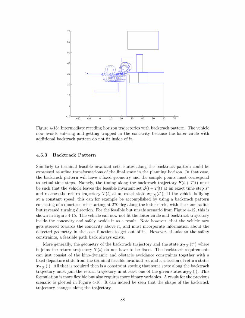
−20 −10 0 10 20 30 40 50 60 70−10
0
10
20
30
40
50
60
70
Figure 4-15: Intermediate receding horizon trajectories with backtrack pattern. The vehiclenow avoids entering and getting trapped in the concavity because the loiter circle withadditional backtrack pattern do not fit inside of it.
4.5.3 Backtrack Pattern
Similarly to terminal feasible invariant sets, states along the backtrack pattern could beexpressed as affine transformations of the final state in the planning horizon. In that case,the backtrack pattern will have a fixed geometry and the sample points must correspondto actual time steps. Namely, the timing along the backtrack trajectory B(t + T |t) mustbe such that the vehicle leaves the feasible invariant set B(t + T |t) at an exact time step s∗
and reaches the return trajectory T (t) at an exact state xT (t)(t∗). If the vehicle is flying
at a constant speed, this can for example be accomplished by using a backtrack patternconsisting of a quarter circle starting at 270 deg along the loiter circle, with the same radiusbut reversed turning direction. For the feasible but unsafe scenario from Figure 4-12, this isshown in Figure 4-15. The vehicle can now not fit the loiter circle and backtrack trajectoryinside the concavity and safely avoids it as a result. Note however, that the vehicle nowgets steered towards the concavity above it, and must incorporate information about thedetected geometry in the cost function to get out of it. However, thanks to the safetyconstraints, a feasible path back always exists.
More generally, the geometry of the backtrack trajectory and the state xT (t)(t∗) where
it joins the return trajectory T (t) do not have to be fixed. The backtrack requirementscan just consist of the kino-dynamic and obstacle avoidance constraints together with afixed departure state from the terminal feasible invariant set and a selection of return statesxT (t)(·). All that is required then is a constraint stating that some state along the backtracktrajectory must join the return trajectory in at least one of the given states xT (t)(·). Thisformulation is more flexible but also requires more binary variables. A result for the previousscenario is plotted in Figure 4-16. It can indeed be seen that the shape of the backtracktrajectory changes along the trajectory.
88

−20 −10 0 10 20 30 40 50 60 70−10
0
10
20
30
40
50
60
70
Figure 4-16: Intermediate receding horizon trajectories with backtrack patterns that arenot geometrically constrained and can join the return trajectory in any one state of a givensubset.
4.5.4 Safe Receding Horizon Planning without Feasibility Guarantees
If one is not interested in maintaining feasibility during all the receding horizon iterations,but only in guaranteeing safety of the vehicle, a practical approach is to simply constrainthe last state of the planning horizon to be the start and end points of a dynamically feasiblepattern with fixed shape. Sample positions along that pattern can again be expressed asaffine transformations of x(t + T |t), either as actual time steps or as regular geometricpoints. No invariance property of the pattern is required, which results in loss of feasibility,but not of safety. Even if the optimization at the next iteration becomes infeasible, thevehicle still has a safe trajectory available that it can execute and that will bring it back towhere it came from.
A scenario of such setup is given in Figures 4-17 and 4-18. The safety pattern againconsists of the 270 deg part of a circle with a reverse quarter circle attached to it. However,to ensure that the start and end points of the safety pattern coincide, an additional linesegment is required of length 2αc||v(T )||, i.e., twice the radius of the loiter circle with entryspeed ||v(T )||. The line segment should be placed between the last state x(t + T |t) of theplanning horizon and the first point on the return arcs. Notice that the pattern scales againwith the entry velocity, adapting the latter to the available space in the environment. Thered triangles along the trajectory in 4-17 indicate positions where the optimization becameinfeasible: the fixed geometric pattern could not be fitted at the end of the trajectory atthe next step. However, the vehicle could just keep moving along the previous solution. Asa result, feasibility was lost for several time steps, but safety was maintained, eventuallyguiding the vehicle past the infeasibilities.
89
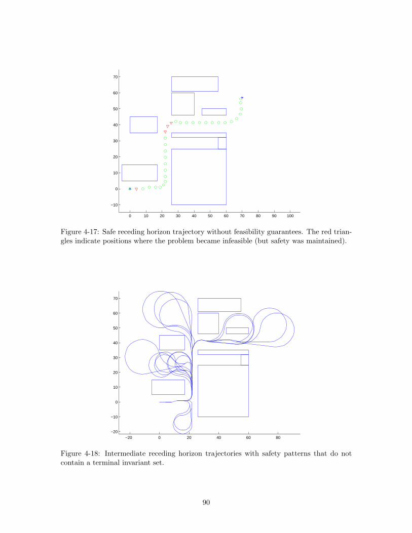
0 10 20 30 40 50 60 70 80 90 100
−10
0
10
20
30
40
50
60
70
Figure 4-17: Safe receding horizon trajectory without feasibility guarantees. The red trian-gles indicate positions where the problem became infeasible (but safety was maintained).
−20 0 20 40 60 80−20
−10
0
10
20
30
40
50
60
70
Figure 4-18: Intermediate receding horizon trajectories with safety patterns that do notcontain a terminal invariant set.
90
4.6 Conclusion
This chapter extended the basic receding trajectory optimization problem to account forfeasibility and safety constraints. Feasibility of the optimization problem at all time stepswas ensured by constraining the intermediate receding horizon trajectories to terminate infeasible invariant sets. These sets can be expressed as affine transformations on the laststate in the horizon and as such are planned online as part of the optimization problem.Examples of a fixed-wing UAV using left and right turning loiter constraints were given.Next, safety was ensured by maintaining feasible backtrack patterns to a return trajectorythat will bring the vehicle back to where it started. A safe receding horizon formulation withfeasibility guarantees was then presented for which simulation results were given. Finally,an alternative safe formulation without feasibility guarantees that is computationally moreefficient was discussed.
91

92

Chapter 5
Safe Distributed TrajectoryPlanning for Multiple Vehicles
This chapter presents an algorithm for provably safe distributed trajectory planning ofmultiple autonomous vehicles that builds on the feasibility concepts developed in Chapter 4.Each vehicle plans its trajectory individually using a receding horizon strategy. Safetyis guaranteed by maintaining, at each time step, dynamically feasible trajectories for allvehicles that terminate in distinct feasible invariant sets. Conflicts between multiple vehiclesare resolved in a sequential, distributed cooperative fashion, in which each vehicle takesinto account the latest trajectory and feasible invariant set of the other vehicles. Besidesmaintaining feasibility, the approach also provides an a priori safe rescue solution if theproblem is too complex to be solved within the time constraints of a real-time system. Thealgorithm is applied to the case of multiple aircraft using loiter patterns as feasible invariantsets. Several examples of conflict situations resolved by the proposed method are presented.
5.1 Introduction
The growing complexity of global air traffic has highlighted the shortcomings of the currentair traffic control infrastructure. In the current system, air traffic controllers use predefinedroutes and standard procedures to ensure safe separation between the aircraft in theirsector. By doing so, maintaining safety remains a manageable problem for the controller;however, the routes followed by the individual aircraft are often suboptimal. For example,the system disallows the aircraft to fly directly to the destination or to take advantageof favorable winds [147]. With the air space becoming more congested, delays are morefrequent and accidents caused by the air traffic controller more likely to occur.
Therefore, in recent years, the concept of Free Flight has emerged, which allows pi-lots to choose their own routes, altitude and speed. Safe conflict detection and resolutionschemes constitute the basis of such a system, and have been a topic of active research.Automating these procedures reduces the risk of human errors and allows for optimizationof the individual aircraft trajectories. Both noncooperative and cooperative conflict reso-lution methods have been proposed. In the noncooperative case, the aircraft involved inthe conflict do not exchange information on their intentions and do not trust one another.Hence, a worst-case approach is adopted. Examples include the work of Tomlin et al., inwhich a game-theoretic method is outlined [147, 146]. Safe protocol-based maneuvers arederived by precomputing reachability sets that account for the uncertainty in the actions of
93
the other aircraft [96, 4]. Although, theoretically, the method can be applied to any numberof aircraft, the computational requirements for more than three aircraft become prohibitive.
In cooperative conflict resolution schemes, the aircraft do exchange information on theirpositions and intentions. Within this class of methods, one can further distinguish be-tween centralized and distributed techniques, depending on whether the conflict is resolvedby a central supervising controller or by each aircraft individually. In the former case, theposition of each aircraft is known to the central controller who designs the individual trajec-tories for all aircraft, typically by solving one large optimization problem. Several central-ized methods with hard anti-collision constraints have been proposed, including approachesbased on semidefinite programming [37], nonlinear programming [108], mixed-integer linearprogramming [127, 114, 103], mixed-integer nonlinear programming [102], and variationalanalysis [53]. However, since the number of inter-vehicle combinations in the planningproblem increases polynomially as n(n− 1)/2 with the number of aircraft n involved in theconflict, the computation times of these methods typically scale exponentially.
By using a receding horizon approach, where the problem is solved over a limited timehorizon that is shifted forward at each iteration, the computation time can be decreased.However, as discussed in Chapter 4, unless the problem is solved to completion at eachiteration – which defeats the purpose of using a receding horizon–, safety is not guaranteed.Namely, the algorithms may fail to provide a solution in future time steps, due to aircraftthat are located beyond the surveillance and planning radius of the aircraft accounted forat the current time step. For instance, when the planning horizon is too short and themaximum turn rate relatively small, the aircraft might approach one another too closelybefore accounting for each other in their plans. As a result, they might not be able to turnaway in time, which would translate into the optimization problem becoming infeasible.
The scaling problem is also apparent in the field of unmanned aerial vehicles. In ap-plications where path planning and coordination of a large fleet of autonomous vehicles isrequired, centralized solutions quickly become computationally intractable. Moreover, inthese applications, the planning problem typically needs to be resolved multiple times, asnew information about the environment is often gathered while the mission unfolds. Thus,a distributed receding horizon planning strategy seems a natural approach to solving themulti-vehicle trajectory generation problem. One such method is proposed in [137], wherestatic obstacles and other moving agents are accounted for by potential functions. Althoughcomputationally attractive, the use of potential functions does not guarantee safety: obsta-cles and other vehicles are captured using soft “constraints” in the cost function. In [55],an alternative algorithm based on an iterative bargaining scheme is given. However, asthe iteration might converge to an infeasible equilibrium, again only soft safety guaranteesexist.
In this chapter, we present a model predictive control framework for distributed, non-iterative cooperative path planning of multiple aircraft with hard safety constraints. Thenovelty lies in the fact that safety is guaranteed by explicitly computing and maintaining asafe trajectory for each aircraft, without having to precompute an invariant set. Moreover,safety can be guaranteed for any number of interacting vehicles. Using the feasible invariantset principle introduced in Chapter 4, this is achieved by ensuring a priori that each aircraftcan always transition to a dynamically feasible loiter pattern that is computed online. Theseloiter patterns act as safe backup paths in case no better solution to a conflict can be foundin time. Conflicts are resolved in a sequential, distributed fashion in which each aircrafttakes into account the latest trajectory and loiter pattern of the other when updating itsown path.
94
Although we are primarily interested in the air traffic control application and the coor-dination problem of multiple fixed-wing UAVs, we present a safe distributed algorithm forautonomous vehicles in general. Afterwards, it is applied to the case of multiple aircraftand MILP is used to compute the trajectories. Note, however, that the algorithm will beformulated independently of the actual trajectory planning method and as such can be usedwith other optimization frameworks as well.
The chapter is organized as follows. Section 5.2 presents the problem formulation andSection 5.3 provides a high level description of the algorithm. Section 5.4 then gives thedetailed MILP formulation with the aircraft model and the loiter and avoidance constraints.Next, Section 5.5 applies the framework to some example scenarios.
5.2 Problem Formulation
5.2.1 Receding Horizon Planning
The general problem tackled in this chapter is that of computing optimal trajectories for aset of (unmanned) vehicles while guaranteeing safety at all times. Each vehicle individuallycomputes its trajectory towards a destination waypoint, accounting for the intentions ofthe other ones. Since information on the other vehicles is gathered online and changes asthey update their trajectories, each vehicle adopts a receding horizon planning strategy.We again assume that the destination of each vehicle i consists of a final position pi,f anda corresponding speed vector vi,f with respect to an inertial coordinate frame. As before,they constitute the final waypoint or state xi,f = [p′
i,f v′i,f ]′.
We will denote the sequence of T +1 states and T inputs resulting from solving the pathplanning problem for vehicle i at a certain time step t respectively as xi(t) and ui(t):
xi(t) =
xi(t|t)xi(t + 1|t)...xi(t + T |t)
, ui(t) =
ui(t|t)ui(t + 1|t)...ui,(t + T − 1|t)
, pi(t) =
pi(t|t)pi(t + 1|t)...pi(t + T |t)
,
where – for notational convenience later on– we denote the position part of the trajectoryseparately as pi(t).
As discussed in Chapter 2, the trajectory starting at time step t must be computedduring time step t − 1, i.e., when the vehicle is on its way to xi(t|t). This state is partof the previous plan, which, as before, we assume to be accurately tracked. As such, thevehicle will be in xi(t|t) when the next plan is executed. This implies that all vehicles canreliably assume that all others are exactly following their trajectories as planned. Includingrobustness to uncertainties in the latter is a topic of current research [70].
In what follows, we will denote the optimization problem for vehicle i that computesthe trajectory starting at time step t as Mi(t). It accounts for the (predicted) initial statexi(t|t), the destination waypoint xi,f , and constraints xi(t + k|t) ∈ X (k) on the states andui(t+k|t) ∈ U(k) on the input commands. We will call a solution acceptable if it is feasibleand its cost lies within a predefined optimality gap.
95
5.2.2 Safety Principle
As was discussed in Chapter 4, feasibility for a single vehicle i can be guaranteed by con-straining the intermediate trajectory xi(t) computed at each time step t to terminate in afeasible invariant set Si(t+T |t) that lies outside of any forbidden zones in the environment.As such, at the next time step t+1, a feasible solution to the trajectory optimization prob-lem is always available a priori, namely, the remaining part of the previous trajectory xi(t)with an extra time step in Si(t + T |t). Hence, if at time step t + 1 no acceptable solutionto the trajectory optimization problem can be found within the timing limits of a hardreal-time guidance system, the previous trajectory can be followed as a safe backup plan.If necessary, the latter can be tracked all the way from time step t to t + T , thus arrivingat the ingress state xi(t + T |t) of the terminal feasible invariant set Si(t + T |t), in whichthe vehicle can remain for an indefinite period of time. In this chapter, with a slight abuseof terminology, we will use the term “safety” for minimal safety, defined as having only aterminal feasible invariant set constraint to maintain feasibility, i.e., we will not account forthe backtrack pattern and return trajectory:
Definition 5.1 (Minimal Safety): We say that a vehicle is in a minimally safe state attime t if from that state, there exists a dynamically feasible, obstacle-free trajectory of Tstates ending in a terminal feasible invariant set S(t + T |t). Minimal safety is then definedas being in such a minimally safe state at all times.
5.2.3 Conflict Description
The principle of maintaining a reachable feasible invariant set is key to ensuring (minimal)safety in case of an encounter between multiple vehicles. It will form the basis of ourdistributed algorithm for safe trajectory planning and conflict resolution. For simplicityof exposition, we will assume that the planning horizons of all vehicles are of equal lengthsame. Extending the algorithm to the more general case of unequal planning horizons canbe done at the cost of a more complicated notation. We start with some definitions:
Definition 5.2 (Conflict Zone): We denote by Ri(t) ⊂ Rn the subset of the inertial space
with dimension n that encompasses the area in which all dynamically feasible trajectories liethat start at xi(t|t) = [p′
i(t|t) v′i(t|t)]′ and end in terminal feasible invariant sets: ∀ui(t) ∈
U = {U(0), . . . ,U(T − 1)} : pi(t) ∪ Si(t + T |t) ⊂ Ri(t). We call Ri(t) the conflict zone ofvehicle i at time step t.
As an initial condition (at t = 0) for the planning and conflict resolution algorithm, wenow assume that none of the conflict zones Ri(0) of the individual vehicles i (i = 1, . . . , K)overlap. As such, at their initial positions pi(0|0), all vehicles can safely plan their individualtrajectories and terminal feasible invariant sets without accounting for the other vehicles.
Assumption 5.1 (Initial Safety): At t=0, we have R1(0)⋂R2(0) . . .
⋂RK(0) = ∅.
When the conflict zones of two or more vehicles start to overlap, however, the individ-ually planned trajectories may intersect and lead to a collision. Therefore, as soon as anoverlap is detected, the corresponding vehicles should account for each other’s trajectorieswhen updating their plans. We call this a conflict, and define it more formally as follows:
Definition 5.3 (Conflict): We say that vehicle i is involved in a conflict Cij(t) with vehiclej 6= i at time step t, if Ri(t) ∩Rj(t) 6= ∅.
96
Since a vehicle i computes the trajectory that starts at time step t during step t − 1,Ri(t) needs to be determined at t− 1 as well, based on the prediction of xi(t|t). To denotethe set of vehicles that are then involved in a conflict with vehicle i at time step t andfor which collision avoidance constraints must be formulated, we introduce the followingnotation:
Definition 5.4 (Avoidance Set): We denote by Ji(t) ⊂ {1, . . . , K} the subset of allvehicles j ∈ {1, . . . , K}, j 6= i, for which Ri(t)∩Rj(t) 6= ∅. We call Ji(t) the avoidance setof vehicle i at time step t.
If two vehicles i and j are involved in a conflict Cij(t), however, their avoidance setsJi(t) and Jj(t) are not necessarily the same: vehicle j can be involved in a conflict Cjk(t)with another vehicle k, but Ri(t) ∩ Rk(t) = ∅. Hence, to maintain safety, vehicle j mustaccount for both i and k, whereas vehicle i only has to account for j. However, althoughthey are not directly in conflict, depending on the order in which the conflict is solved, thetrajectory of i may still be influenced by that of k through the effect that k has on thetrajectory of j. We therefore introduce the following set:
Definition 5.5 (Conflict Set): We denote by Di(t) ⊂ {1, . . . , K} the subset of all vehiclesj ∈ {1, . . . , K} for which there exists a vehicle sequence k1, . . . , kS such that Ri(t)∩Rk1
(t) 6=∅, Rk1
(t) ∩ Rk2(t) 6= ∅, . . . ,RkD
(t) ∩ Rj(t) 6= ∅. We call Di(t) the conflict set of vehicle iat time step t.
Note that if j ∈ Di(t), we have Dj(t) = Di(t). Hence, we can define one set D(t) ≡ Di(t)that groups all vehicles that are connected through a chain of conflicts Cik1
(t), . . . , CkDj(t)at time step t. Any vehicles that are not do not belong to D(t) will not come into playin resolving the conflict involving the vehicles in D(t). Hence, without loss of generality,we can restrict ourselves to solving the case of a single conflict C(t) associated with D(t).Other conflict sets may exist in the environment that can all be considered independent ofeach other.
By considering the vehicles in D(t) as vertices that are connected by an edge if a conflictCij(t) between a pair (i, j) exists, a graph can be associated with the conflict set D(t) thatrepresents the inter-vehicle dependence at time step t. We define this graph as the conflictgraph G(t):
Definition 5.6 (Conflict Graph): We denote by G(t) the connected graph associated withconflict set D(t) at time step t that results from considering vehicles as vertices and edges asfollows: a pair of vertices (i, j) is connected if there exists a conflict Cij(t) between vehiclesi and j at time step t.
Independent conflict sets thus correspond to disconnected conflict graphs. Note that becausethe vehicles are moving, the conflict sets and associated conflict graphs may change at eachtime step. The planning algorithm proposed in this chapter will automatically account forthis.
5.2.4 Communication Requirements
To determine the structure of the conflict graph there has to exist a communication networkbetween the vehicles in the conflict sets. One possible communication strategy is to havetwo vehicles communicate with each other as soon as they detect each other within theirconflict zones. Alternatively, all vehicles only communicate with a central hub (either a
97
ground station or leader vehicle) that keeps track of the positions pi(t) and conflict zonesRi(t) of all vehicles i at all time steps t. Using this information it can determine theconflict set D(t) and corresponding conflict graph G(t), and communicate the avoidancesets Ji(t) back to the respective vehicles i. An additional benefit is that it can maintainthe clocks of all vehicles synchronized, which will be crucial in the conflict resolution partof the algorithm.
Assumption 5.2 (Central Hub): We assume that a central hub H is present with whichall vehicles i = 1, . . . , K communicate. It keeps the clocks of all vehicles synchronized, anddetermines the avoidance sets Ji(t), the conflict set D(t), and the corresponding conflictgraph G(t).
Although the existence of a central hub is not crucial to our safety framework, it simplifiesthe required communication infrastructure and the presentation of the algorithm. Theactual trajectory optimization will still be done in a distributed fashion, regardless of howinformation is exchanged between the vehicles. Decentralizing the communication itself isan ad hoc networking problem for which multiple techniques exist [121, 145].
To avoid collisions, vehicle i needs to account for the position sequence pj(t) of allvehicles j ∈ Ji(t) when solving its trajectory optimization problem Mi(t). Moreover, tomaintain future feasibility, its terminal feasible invariant set Si(t+T |t) should not intersectwith any of the terminal feasible invariant sets Sj(t + T |t) of the vehicles j ∈ Ji(t). ForMILP-based trajectory planning, it suffices to describe all sets Sj(t+T |t) by the coordinatesof a surrounding rectangular box which will then be considered a forbidden zone by vehiclei.
To solve its trajectory optimization problem Mi(t), vehicle i thus needs to obtain thelatest trajectory information of all vehicles j ∈ Ji(t), and vice versa, the latter need toknow the trajectory of i. Hence, either communication links between all vehicles in Ji(t)and vehicle i need to be set up, or the information can be distributed via the central hub.We now introduce the following notation to capture this trajectory information:
Definition 5.7 (Plan): We denote by Pi(t) the sequence pi(t) of trajectory points startingat time step t and the coordinates of a rectangular box that surrounds the terminal feasibleinvariant set Si(t + T |t) of vehicle i. We call Pi(t) the plan of vehicle i at time step t.
The plans Pj(t) for all vehicles j ∈ Ji(t) can then be included as avoidance constraints in thetrajectory optimization problem Mi(t). We will denote this as the problem Mi(t) s.t. Pj(t),∀j ∈ Ji(t).
A key step in our conflict resolution algorithm is that the vehicles in D(t) need to decideon an order O(t) in which each one updates its trajectory at time step t− 1. An importantproperty of the conflict graph G(t) is that vehicles that are not in direct conflict with eachother, i.e., vehicle vertices that have no edge that directly connects them, can computetheir trajectories simultaneously without affecting each other’s feasibility. Indeed, sincetheir conflict zones at the current time step do not overlap, their updated trajectories willnot intersect.
In our algorithm, distinct subsets of such unconnected vehicle nodes will be allocatedsequential time slots during which all vehicles of a particular subset optimize their individualtrajectories simultaneously. To allocate as much computation time as possible to eachvehicle, we therefore need to determine the minimum number of such unconnected vehiclesubsets in D(t). This corresponds to a vertex coloring problem for the conflict graph G(t).
98
The goal is to assign colors c(i) to each vertex i of G(t) such that no two vertices of the samecolor are directly connected while minimizing the number of colors for the entire graph.Brute-force algorithms could be used to find a minimum coloring, but Brelazs heuristicalgorithm provides a good solution in faster time [23]. We will not elaborate further onsuch algorithms – see [70] for more details,– and will assume that the vehicles or the centralhub can determine an appropriate coloring of the conflict graph G(t) and correspondingpartitioning of the conflict set D(t) in subsets Fc(t). Instead, we will focus on the timingand safety properties of the trajectory planning algorithm. We summarize as follows:
Definition 5.8 (Conflict Subsets): We denote by Fc(t), c = 1, . . . , NG(t) the non-inter-secting subsets of the conflict set D(t) resulting from solving a vertex coloring problem ofthe corresponding conflict graph G(t) at time step t. We call these subsets conflict subsets.In the minimal case, the number of conflict subsets NG(t) is the chromatic number of thegraph.
Once a coloring and conflict partitioning have been determined, a computation orderand corresponding time slots need to be assigned to the various conflict subsets. At eachtime step t, we therefore introduce time slots of length ∆tcomp(t) = ∆t/NG(t) where ∆t isthe discretization step of the receding horizon. In our algorithm, each vehicle will have atleast a time ∆tcomp(t) available to solve its trajectory planning problem. Notice, however,that some vehicles can make use of more time slots without taking time away from othervehicles. For example, vehicles i whose avoidance sets Ji(t) contain only vehicle vertices j ofthe same color can use the rest of the time step to optimize their trajectories after vehiclesj used the previous time slot. Hence, all vehicles of a particular conflict subset Fc(t) willthus start optimizing at the same time, but are not necessarily allocated the same numberof time slots. All have at least one slot of length ∆tcomp(t) available, however.
The previous insight leads us to the conclusion that there must exist an optimal orderamong the conflict subsets that maximizes the number of vehicles that can be allocatedmore than one time slot while ensuring that all vehicles get at least one slot. A goodheuristic is to start with the conflict subset that is the most connected, i.e., the one forwhich the union of the avoidance sets of its members is the largest. Note, however, thatthis is not necessarily the largest conflict subset. We again assume that the central hubdetermines this order of the vehicle subsets and assigns the start and number of time slotsto each individual vehicle:
Assumption 5.3 (Conflict Order): We assume that the central hub H can determine anorder O(t) = {ord(c), c = 1, . . . , NG(t)} among the conflict subsets Fc(t), and a correspond-ing sequence of non-overlapping time slots {[tord(c),s, tord(c),f + ∆tcomm), c = 1, . . . , NG(t)}that allocate the start time tord(c),s and end time tord(c),f during which the vehicles in theconflict set with order number ord(c) should solve their trajectory optimization problemsat time step t − 1. ∆tcomm is the time required to broadcast the plan Pi(t) of a vehi-cle i ∈ Fc(t) to the vehicles in its avoidance set Ji(t). We assume that this time is thesame for all vehicles. If Ji(t) only contains vehicles j that have ord(c(j)) < ord(c(i))then vehicle i can occupy the remainder of the time step and will be allocated a time slot[tord(c(i)),s, (t− 1−∆tcomm) + ∆tcomm). In both cases, we will denote the allocated time slotfor vehicle i as [tord(c(i)),s, ti,f + ∆tcomm).
Since a vehicle may leave the conflict set, or a new one may enter, the central hub mustredetermine D(t) and O(t) at every time step. Using the preceding definitions, we can
99
now formulate a distributed optimization strategy for safe trajectory planning and conflictresolution.
5.3 Safe Trajectory Planning Algorithm
5.3.1 Algorithm
Starting at t = 0, at each following time step t, let all vehicles i in the environment(i = 1, . . . , K) execute the following planning algorithm:
Start: Start at time t.
• Step 1: Predict the next state xi(t + 1) and send it to the central hub H. Next,receive the avoidance set Ji(t+1) with conflict order numbers ord(c(j)) of all vehiclesj ∈ Ji(t + 1) and the time slot (tord(c(i)),s, ti,f ) from H.
• Step 2a: If Ji(t + 1) 6= ∅, broadcast the current plan Pi(t) to all vehicles in Ji(t + 1)and go to Step 3. Else, go to Step 2b.
• Step 2b: Solve Mi(t + 1). If an acceptable solution xi(t + 1) ∪ Si(t + T + 1|t + 1) isfound before time t + 1, let the new plan Pi,t+1 = pi(t + 1)∪Si(t + T + 1|t + 1). Else,let Pi(t + 1) = Pi(t) \ pi(t). Go to End.
• Step 3: At time tord(c(i)),s, solve Mi(t + 1) s.t. Pj(t + 1), j ∈ Ji(t + 1) : ord(c(j)) <ord(c(i)) and s.t. Pk(t), k ∈ Ji(t + 1) : ord(c(k)) > ord(c(i)).
• Step 4: If an acceptable solution xi(t + 1)∪Si(t + T + 1|t + 1) is found at ti,f , let thenew plan Pi(t + 1) = pi(t + 1)∪Si(t + T + 1|t + 1) . Else, let Pi(t + 1) = Pi(t) \pi(t).
• Step 5: During (ti,f , ti,f + ∆tcomm), broadcast Pi(t + 1) to all vehicles k ∈ Ji(t + 1) :ord(c(k)) > ord(c(i)).
End: End by time t + 1, and repeat.
By construction, this algorithm maintains minimal safety for all vehicles: at each timestep, there exists, a priori, a collision-free dynamically feasible trajectory for each vehicle.Namely, since all other vehicles during their last update accounted for the latest plan of thevehicle that is currently planning, the remaining part of its previous trajectory ending in afeasible invariant set can always be used as a safe “backup” plan. We formalize this in thefollowing theorem:
Theorem 5.1: Given a conflict-free situation at time t = 0 (Assumption 5.1), the aboveplanning algorithm will maintain minimally safe trajectories (according to Definition 5.1)for all vehicles i = 1, . . . , K at all time steps.
Proof : We prove the minimal safety property by using a double induction argument overthe sequence of time steps and over the sequence of conflict subsets within a time step. ByAssumption 1, at t = 0, all vehicles are in a minimally safe state (as defined in Definition 5.1)and
⋂
i=1...K Ri(0) = ∅. Hence, by definition of Ri(0), all vehicles i have non-intersectingplans at t = 0. They thus all have an a priori minimally safe trajectory available at t = 1,namely, Pi(0)\pi(0) ending in non-intersecting terminal feasible invariant sets Si(t + T |t)at time step T , the length of the planning horizon.
100
Assume now that at time step t = k, all vehicles have safe plans Pi(k). Before computingits next plan Pi(k + 1), a particular vehicle i will know whether its avoidance set Ji(k + 1)is empty or not by communicating with the central hub H (Step 1). In case Ji(k + 1) = ∅,any feasible solution to Mi(k + 1) will be minimally safe, since the conflict zone Ri(k + 1)does not intersect with that of any other vehicles. If an acceptable solution cannot be foundin time, Pi(k)\pi(k), i.e. the previous plan excluding the current state, is still valid andavailable as a minimally safe backup plan at time step k + 1.
In case Ji(k + 1) 6= ∅, vehicle i will obtain its order number ord(c(i)) ∈ {1 . . . NG(k+1)}from the central hub H. If ord(c(i)) = 1, vehicle i is the first to update its trajectory at timestep k, along with all other vehicles in the conflict subset Fc(i)(k + 1). Given that the planPi(k) was minimally safe, a minimally safe solution to Mi(k+1) s.t. Pj(k+1),∀j ∈ Ji(k+1)continues to exist, namely, Pi(k)\pi(k). In the nominal case, Pi(k + 1) will differ fromPi(k)\pi(k). Since the updated plan Pi(k+1) is constrained to avoid the existing trajectoriesPj(k),∀j ∈ Ji(k +1), all other vehicles in the conflict set D(k +1) remain in minimally safestates. The same reasoning holds for all other vehicles s in the conflict subset Fc(i)(k + 1).Since, per definition of Fc(i)(k +1), their avoidance sets Js(k +1) do not contain any of theother vehicles with ord(c(s)) = 1 = ord(c(i)), their plans will not affect each other.
Now, consider a vehicle i′ with ord(c(i′)) > 1, and assume that it has a minimally safebackup plan Pi′(k)\pi′(k). It will account 1) for the previous plans Pj′(k) for all followingvehicles j′ ∈ Ji′(k + 1) : ord(c(j′)) > ord(c(i′)) and 2) for the new plans Pl′(k + 1) ofall prior vehicles l′ ∈ Ji′(k + 1) : ord(c(l′)) < ord(c(i′)). Given that a minimally safeplan Pi′(k)\pi′(k) for vehicle i′ exists, the problem is feasible. Thus 1) all vehicles j′ withord(c(j′)) > ord(c(i′)) will still have minimally safe backup plans Pj′(k)\pj′(k) availablewhen they update their paths, and 2) the new plans Pl′(k + 1) of all vehicles l′ withord(c(l′)) < ord(c(i′)) will remain minimally safe. Again, the same reasoning holds for allother vehicles s′ in the conflict subset Fc(i′)(k + 1). Because their avoidance sets Js′(k + 1)do not contain any of the other vehicles with ord(c(s′)) = ord(c(i′)), their plans will notaffect each other.
Hence, by induction over the sequence of conflict subsets, minimal safety for all vehiclesis maintained within time step k. As a result, each vehicle is in a minimally safe state atthe start of the next time step k + 1. Thus, using induction once more, given the safetyassumption at t = 0, minimal safety for all vehicles is maintained over the sequence of timesteps.
5.3.2 Remarks
1. Note that the algorithm is not a bargaining or convergence process: at any given timestep, each vehicle contributes only once to the solution of the conflict. As presented here, thealgorithm should cycle through the full conflict set D(t+1) before the next time step t+1, i.e.,the time at which all vehicles reach the first state in their plans. However, the more vehiclesthat are involved in the conflict graph, the longer each vehicle will typically take to solve itstrajectory optimization problem. On the other hand, the allocated computation time scalesinversely with the number of conflict subsets (i.e., colors). Therefore, if necessary, for aparticular cycle of the algorithm, the central hub can distribute the computation times overseveral time steps. If during this cycle of longer duration all other vehicles keep tracking thelatest trajectories that they communicated, safety for all vehicles is maintained. This is onlythe case, however, if no new vehicles enter the conflict set during that longer cycle. Sinceone iteration of the conflict resolution algorithm is now spread over more than one time
101
step, this can be guaranteed by computing conflict sets and subsets for longer planninghorizons in Step 1 of the algorithm. Alternatively, the central hub could command thenew vehicle not to update its plan and to keep following its latest trajectory, while itcommunicates this latest plan to the other vehicles. The latter can then still include thatplan as an avoidance constraint in their respective trajectory optimizations, without makingthe problem infeasible.
2. Worst-case, if many vehicles are involved in the conflict graph, and the problembecomes too complex to be solved within the timing constraints of the algorithm, the vehicleswill enter their (non-intersecting) terminal feasible invariant sets and may get trapped init. This could also happen if the problem has certain geometric symmetries. In bothcases, however, the central hub can then decide on subsequent subsets of the conflict sets(including the possibility of one by one) and allocate as much time as needed to compute away out of the feasible invariant sets or break the symmetry. Such live-lock situations andthe associated instability of not reaching the goal are primarily related to the cost function.Here, however, we are only concerned about guaranteeing feasibility. Typically, feasibilityneeds to be ensured before stability can be tackled and is therefore a problem of interestby itself. Ensuring stability to build a provably stable algorithm is still a topic of ongoingresearch [70].
3. It is natural to assume that the vehicles in the first conflict subset in the conflict orderare favored because they can update their trajectories first. However, in our simulationsthis was not necessarily the case: we generally found that most vehicles have to make equalefforts (in terms of deviating from their nominal trajectories towards their destination) toresolve the conflict. Depending on the geometry of the individual trajectories, the firstvehicle could even be more constrained than the last one in the order sequence. Moreover,by randomly changing the conflict subset order at each time step, no single vehicle shouldhave an a priori advantage over any other.
4. The algorithm is robust to communication failures. As soon as a broken communica-tion link is detected, the vehicles involved should execute their backup plans: they shouldkeep following the trajectory that was last broadcast and eventually enter their terminalfeasible invariant sets. The other vehicles can then keep accounting for those same planswhen updating their trajectories.
5. The formulation of the actual trajectory optimization problem should account forthe discrete-time nature of the conflict resolution algorithm: its constraints must guaranteecollision avoidance during the continuous transition between the discrete trajectory samplepoints.
5.4 Implementation Using MILP
Although the conflict resolution algorithm can be used with other trajectory optimizationtechniques, we use MILP again to formulate the avoidance constraints and express therequirements for the feasible invariant sets. In the following, the framework is applied tothe case of multiple aircraft using the loiter patterns from Chapter 4 as terminal feasibleinvariant sets. To highlight the performance of the conflict resolution algorithm, we present2D scenarios. However, the algorithm can readily be used with 3D problems as well. Theaircraft would then have an extra degree of flexibility, namely a change in altitude, to plannon-intersecting loiter patterns.
102
5.4.1 Aircraft Model
For our simulations, we use a 2D version of the first-order reference velocity model (3.15)from Section 3.4 that captures the dynamics of an actual aircraft more accurately than thedouble integrator model used in Chapters 2 and 4. Let pi(t) = [xi(t) yi(t)]
′ and vi(t) =[xi(t) yi(t)]
′ denote the inertial position and velocity vector again. As in (3.15), let thecontrol input to aircraft i be the inertial reference speed vector ui(t) = [xcmd,i(t) ycmd,i(t)]
′.The 2D version of the velocity control model (3.15) then becomes:
xi(t) = − 1τi
xi(t) + ki
τixcmd,i(t)
yi(t) = − 1τi
yi(t) + ki
τiycmd,i(t)
(5.1)
in which τi is again a time constant and ki is a gain. In state space form, xi(t) = Aixi(t)+Biui(t), we obtain:
xi(t)yi(t)xi(t)yi(t)
=
0 0 1 00 0 0 10 0 − 1
τi0
0 0 0 − 1τi
xi(t)yi(t)xi(t)yi(t)
+
0 00 0
ki
τi0
0 ki
τi
[
xcmd,i(t)ycmd,i(t)
]
(5.2)
Using the bilinear transform with a discretization step ∆t, the discrete-time model becomes:
xi(k + 1)yi(k + 1)xi(k + 1)yi(k + 1)
=
1 0 ∆t2
(
1 + 2τi−∆t2τi+∆t
)
0
0 1 0 ∆t2
(
1 + 2τi−∆t2τi+∆t
)
0 0 2τi−∆t2τi+∆t
0
0 0 0 2τ−∆t2τi+∆t
xi(k)yi(k)xi(k)yi(k)
+
ki(∆t)2
2τi+∆t0
0 ki(∆t)2
2τi+∆t2ki∆t
2τi+∆t0
0 2ki∆t2τi+∆t
[
xcmd,i(k)ycmd,i(k)
]
(5.3)
The magnitudes of the reference and actual inertial velocity are again bounded by aminimum required speed vmin,i and a maximum achievable speed vmax,i:
vmin,i ≤ ||vi(t)|| ≤ vmax,i
vmin,i ≤ ||ui(t)|| ≤ vmax,i(5.4)
To capture limits on turn rate and differences in the lateral and longitudinal aircraft dy-namics, we reuse constraints (3.20a-b):
||ai(t) − αivi(t)vi(0)
|| ≤ βi
||ai(t) + αivi(t)vi(0)
|| ≤ βi
||ai(t)|| ≤ alat,max,i
(5.5)
where αi and βi are given by expressions (3.21a-b). Remember that these inequalitiesapproximate the geometric profile that encompasses all inertial acceleration vectors ai =[xi yi]
′ that are dynamically feasible. For the linearized and discrete time version of con-
103
straints (5.4) and (5.5), we refer the reader back to Section 3.4.
5.4.2 Loiter Circles
As discussed in Section 5.2, the trajectory at each iteration is constrained to terminate ina feasible invariant set. Like the examples in Chapter 4, we choose this to be a right or leftturning loiter circle (see Figure 4-3), where the turn direction will be decided upon by the op-timization problem. Remember that the loiter pattern was described by equally spaced sam-ple points pR(θ) and pL(θ) along the circles. By introducing a rotation matrix R(θ), thesepoints were expressed as affine transformations of the last state xi(T ) = [pi(T )′ vi(T )′]′ inthe planning horizon:
pR,i(θ) = pi(T ) + αc,i(R(θ) − I)v⊥i (T ) (5.6)
pL,i(θ) = pi(T ) − αc,i(R(θ) − I)v⊥i (T ) (5.7)
The state xi(T ) thus acts as an entry state to the loiter circles of which the radius scaleslinearly with the magnitude of the entry velocity vi(T ). As such, by slowing down orspeeding up, the aircraft has the flexibility to adapt the size of its loiter circle to the stateof the environment, i.e., to the trajectories and locations of the loiter patterns of the otheraircraft. In the following, these geometric relations will be used to express the avoidanceconstraints.
5.4.3 Avoidance Constraints
We assume here for simplicity that the conflict zone Ri of all aircraft i is a circle offixed radius rreach, where rreach is the maximum distance that can be traveled over thelength of the planning horizon, including a margin for the loiter circle. Denoting the ra-dius of the loiter circle when flying at vmax by rmax, a simple calculation yields rreach =√
(T∆tvmax + rmax)2 + 4r2max. Note that this is the most conservative assumption: in gen-
eral, an aircraft might not be able to reach the full area covered by the circle, and the shapeof the conflict zone will typically depend on the initial velocity vi(0). Furthermore, theradius will be different depending on the length of the planning horizon and the velocityand turn rate bound.
The avoidance set Ji can then easily be determined: it consists of all aircraft that arewithin a distance of 2rreach of aircraft i at time step t. In addition, Assumption 5.1 reducesto all aircraft being separated by a distance greater than 2rreach: ∀i, j ∈ {1, . . . , K}, i 6= j :‖pi(0) − pj(0)‖ > 2rreach. As discussed in Steps 2a and 5 of the trajectory planning andconflict resolution algorithm, when the conflict set D 6= ∅, the aircraft will communicatetheir plans P to one another. Since we assumed that all vehicles can accurately followthe planned trajectories, their waypoints and loiter circles can be considered as translatingobstacles with known motion by the aircraft that is currently planning. These constraintsare now specified in more detail.
Regular Trajectory Points
Each trajectory point pj(k) of aircraft j ∈ Ji is considered an obstacle that is present attime step k in the planning horizon, if that point lies in the conflict zone Ri of the planningaircraft i, i.e., when pj(k) ∈ Ri. Denote the set of time steps for which the latter holdsas Tj ⊆ T = [0, . . . , T ]. Due to the discrete-time nature of the trajectories, the waypoints
104

are considered square obstacles of dimension 2ds = 2(max(vmax∆t, dsafe)+ vmax∆t), wheredsafe is the required safety distance around each aircraft. The lower left corner of thewaypoint obstacle pj(k) = (xj(k), yj(k)) is then given by (xmin,jk, ymin,jk) = (xj(k) −ds, yj(k) − ds), the upper right corner by (xmax,jk, ymax,jk) = (xj(k) + ds, yj(k) + ds).
For the trajectory points (xi(k), yi(k)), k ∈ Tj – which include points on the loiterpattern if the aircraft is using its backup plan,– the required safety distance with all otheraircraft is then guaranteed at all times during the planning horizon, if these points satisfythe following set of constraints:
∀j ∈ Ji, ∀k ∈ Tj :
xi(k) ≤ xmin,jk + Mbj1(k)−xi(k) ≤ −xmax,jk + Mbj2(k)
yi(k) ≤ ymin,jk + Mbj3(k)−yi(k) ≤ −ymax,jk + Mbj4(k)
4∑
n=1
bjn(k) ≤ 3
bjn(k) ∈ {0, 1}
(5.8)
As in previous chapters, bjn(k) are binary variables and M is a sufficiently large positivenumber. The last constraint again ensures that at least one of the inequality constraints isactive, thereby guaranteeing that the trajectory point (xi(k), yi(k)) lies outside the waypointobstacles of the other aircraft.
Loiter Points
To ensure that the loiter circle of the planning aircraft i does not intersect with that of anyof the aircraft j ∈ Ji, we derive equivalent constraints for the sample points along the circle.Assume that there are NL = ⌈2π
θs⌉ of these, where θs denotes the discretization angle. Let
the loiter circle of each aircraft j ∈ Ji be contained within a square with lower left corner(xmin,jL, ymin,jL) and upper right corner (xmax,jL, ymax,jL). As discussed in Chapter 4,these dimensions include a safety boundary that accounts for the continuous segments ofthe loiter circle of aircraft i between its discrete sample points. The two corner points,together with the time step at which the loiter is initiated, is the only information thatneeds to be exchanged about the loiter pattern.
The square that needs to be avoided by the loiter points of the planning aircraft i cannow be considered a static obstacle. By introducing a binary variable d that selects eitherthe right or left circle, and by substituting expressions (5.6)-(5.7) for the sample points inthe avoidance constraints (5.8), we obtain:
∀j ∈ Ji, ∀l ∈ [1, . . . , NL] :
xi(T ) − αc (cos lθs − 1) yi(T ) − αc (sin lθs) xi(T ) ≤ xmin,jL + Mbjl1 + Md−xi(T ) + αc (cos lθs − 1) yi(T ) + αc (sin lθs) xi(T ) ≤ −xmax,jL + Mbjl2 + Md
yi(T ) − αc (sin lθs) yi(T ) + αc (cos lθs − 1) xi(T ) ≤ ymin,jL + Mbjl3 + Md−yi(T ) + αc (sin lθs) yi(T ) − αc (cos lθs − 1) xi(T ) ≤ −ymax,jL + Mbjl4 + Md
(5.9)
105
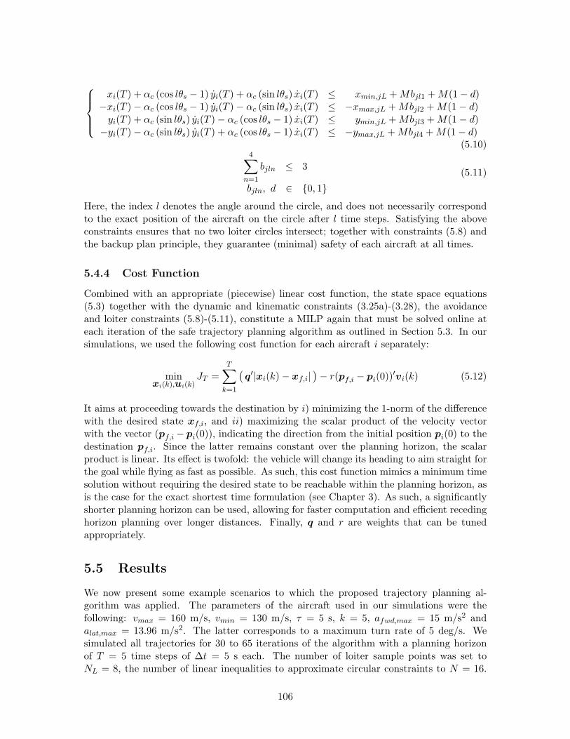
xi(T ) + αc (cos lθs − 1) yi(T ) + αc (sin lθs) xi(T ) ≤ xmin,jL + Mbjl1 + M(1 − d)−xi(T ) − αc (cos lθs − 1) yi(T ) − αc (sin lθs) xi(T ) ≤ −xmax,jL + Mbjl2 + M(1 − d)
yi(T ) + αc (sin lθs) yi(T ) − αc (cos lθs − 1) xi(T ) ≤ ymin,jL + Mbjl3 + M(1 − d)−yi(T ) − αc (sin lθs) yi(T ) + αc (cos lθs − 1) xi(T ) ≤ −ymax,jL + Mbjl4 + M(1 − d)
(5.10)4
∑
n=1
bjln ≤ 3
bjln, d ∈ {0, 1}(5.11)
Here, the index l denotes the angle around the circle, and does not necessarily correspondto the exact position of the aircraft on the circle after l time steps. Satisfying the aboveconstraints ensures that no two loiter circles intersect; together with constraints (5.8) andthe backup plan principle, they guarantee (minimal) safety of each aircraft at all times.
5.4.4 Cost Function
Combined with an appropriate (piecewise) linear cost function, the state space equations(5.3) together with the dynamic and kinematic constraints (3.25a)-(3.28), the avoidanceand loiter constraints (5.8)-(5.11), constitute a MILP again that must be solved online ateach iteration of the safe trajectory planning algorithm as outlined in Section 5.3. In oursimulations, we used the following cost function for each aircraft i separately:
minxi(k),ui(k)
JT =T
∑
k=1
(
q′|xi(k) − xf,i|)
− r(pf,i − pi(0))′vi(k) (5.12)
It aims at proceeding towards the destination by i) minimizing the 1-norm of the differencewith the desired state xf,i, and ii) maximizing the scalar product of the velocity vectorwith the vector (pf,i − pi(0)), indicating the direction from the initial position pi(0) to thedestination pf,i. Since the latter remains constant over the planning horizon, the scalarproduct is linear. Its effect is twofold: the vehicle will change its heading to aim straight forthe goal while flying as fast as possible. As such, this cost function mimics a minimum timesolution without requiring the desired state to be reachable within the planning horizon, asis the case for the exact shortest time formulation (see Chapter 3). As such, a significantlyshorter planning horizon can be used, allowing for faster computation and efficient recedinghorizon planning over longer distances. Finally, q and r are weights that can be tunedappropriately.
5.5 Results
We now present some example scenarios to which the proposed trajectory planning al-gorithm was applied. The parameters of the aircraft used in our simulations were thefollowing: vmax = 160 m/s, vmin = 130 m/s, τ = 5 s, k = 5, afwd,max = 15 m/s2 andalat,max = 13.96 m/s2. The latter corresponds to a maximum turn rate of 5 deg/s. Wesimulated all trajectories for 30 to 65 iterations of the algorithm with a planning horizonof T = 5 time steps of ∆t = 5 s each. The number of loiter sample points was set toNL = 8, the number of linear inequalities to approximate circular constraints to N = 16.
106
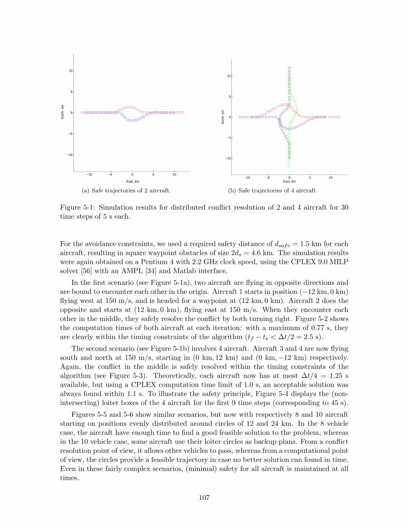
−10 −5 0 5 10
−10
−5
0
5
10
East, km
Nor
th, k
m
(a) Safe trajectories of 2 aircraft.
−10 −5 0 5 10
−10
−5
0
5
10
East, km
Nor
th, k
m
(b) Safe trajectories of 4 aircraft.
Figure 5-1: Simulation results for distributed conflict resolution of 2 and 4 aircraft for 30time steps of 5 s each.
For the avoidance constraints, we used a required safety distance of dsafe = 1.5 km for eachaircraft, resulting in square waypoint obstacles of size 2ds = 4.6 km. The simulation resultswere again obtained on a Pentium 4 with 2.2 GHz clock speed, using the CPLEX 9.0 MILPsolver [56] with an AMPL [34] and Matlab interface.
In the first scenario (see Figure 5-1a), two aircraft are flying in opposite directions andare bound to encounter each other in the origin. Aircraft 1 starts in position (−12 km, 0 km)flying west at 150 m/s, and is headed for a waypoint at (12 km, 0 km). Aircraft 2 does theopposite and starts at (12 km, 0 km), flying east at 150 m/s. When they encounter eachother in the middle, they safely resolve the conflict by both turning right. Figure 5-2 showsthe computation times of both aircraft at each iteration: with a maximum of 0.77 s, theyare clearly within the timing constraints of the algorithm (tf − ts < ∆t/2 = 2.5 s).
The second scenario (see Figure 5-1b) involves 4 aircraft. Aircraft 3 and 4 are now flyingsouth and north at 150 m/s, starting in (0 km, 12 km) and (0 km,−12 km) respectively.Again, the conflict in the middle is safely resolved within the timing constraints of thealgorithm (see Figure 5-3). Theoretically, each aircraft now has at most ∆t/4 = 1.25 savailable, but using a CPLEX computation time limit of 1.0 s, an acceptable solution wasalways found within 1.1 s. To illustrate the safety principle, Figure 5-4 displays the (non-intersecting) loiter boxes of the 4 aircraft for the first 9 time steps (corresponding to 45 s).
Figures 5-5 and 5-6 show similar scenarios, but now with respectively 8 and 10 aircraftstarting on positions evenly distributed around circles of 12 and 24 km. In the 8 vehiclecase, the aircraft have enough time to find a good feasible solution to the problem, whereasin the 10 vehicle case, some aircraft use their loiter circles as backup plans. From a conflictresolution point of view, it allows other vehicles to pass, whereas from a computational pointof view, the circles provide a feasible trajectory in case no better solution can found in time.Even in these fairly complex scenarios, (minimal) safety for all aircraft is maintained at alltimes.
107
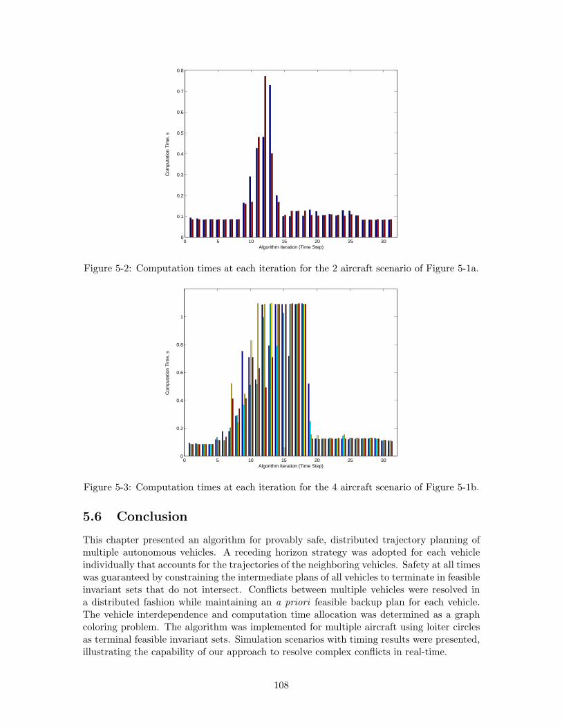
0 5 10 15 20 25 300
0.1
0.2
0.3
0.4
0.5
0.6
0.7
0.8
Algorithm Iteration (Time Step)
Com
puta
tion
Tim
e, s
Figure 5-2: Computation times at each iteration for the 2 aircraft scenario of Figure 5-1a.
0 5 10 15 20 25 300
0.2
0.4
0.6
0.8
1
Algorithm Iteration (Time Step)
Com
puta
tion
Tim
e, s
Figure 5-3: Computation times at each iteration for the 4 aircraft scenario of Figure 5-1b.
5.6 Conclusion
This chapter presented an algorithm for provably safe, distributed trajectory planning ofmultiple autonomous vehicles. A receding horizon strategy was adopted for each vehicleindividually that accounts for the trajectories of the neighboring vehicles. Safety at all timeswas guaranteed by constraining the intermediate plans of all vehicles to terminate in feasibleinvariant sets that do not intersect. Conflicts between multiple vehicles were resolved ina distributed fashion while maintaining an a priori feasible backup plan for each vehicle.The vehicle interdependence and computation time allocation was determined as a graphcoloring problem. The algorithm was implemented for multiple aircraft using loiter circlesas terminal feasible invariant sets. Simulation scenarios with timing results were presented,illustrating the capability of our approach to resolve complex conflicts in real-time.
108
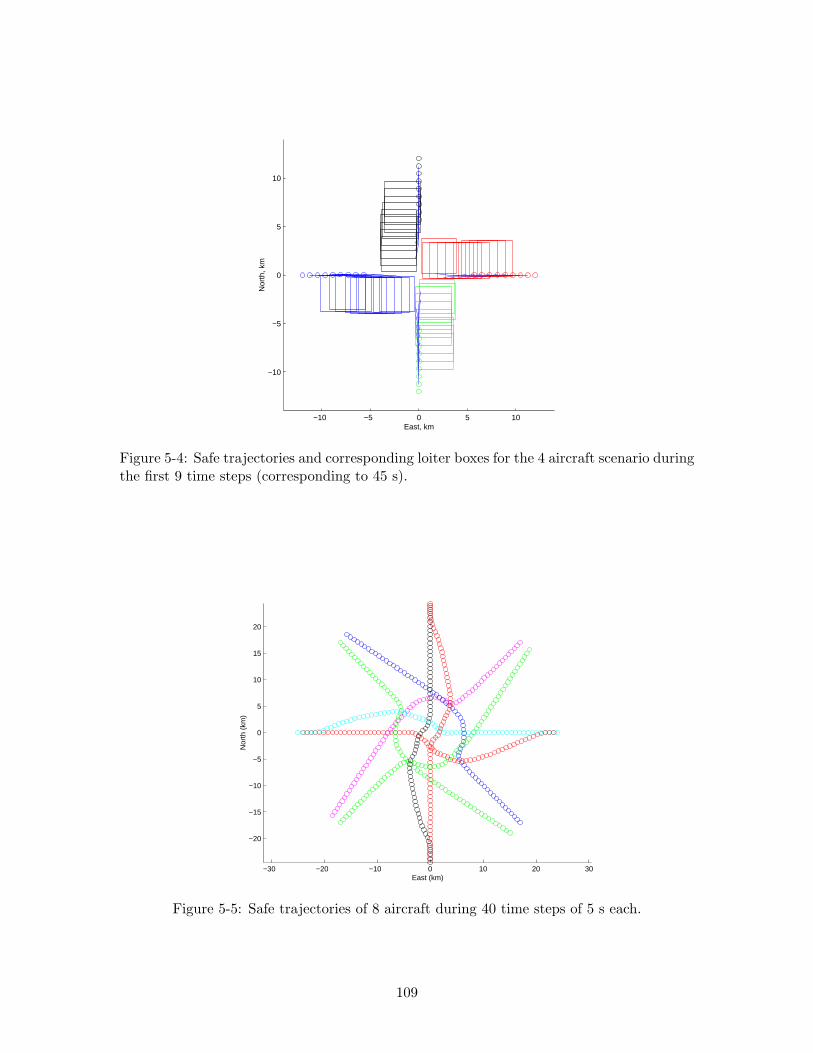
−10 −5 0 5 10
−10
−5
0
5
10
East, km
Nor
th, k
m
Figure 5-4: Safe trajectories and corresponding loiter boxes for the 4 aircraft scenario duringthe first 9 time steps (corresponding to 45 s).
−30 −20 −10 0 10 20 30
−20
−15
−10
−5
0
5
10
15
20
East (km)
Nor
th (
km)
Figure 5-5: Safe trajectories of 8 aircraft during 40 time steps of 5 s each.
109
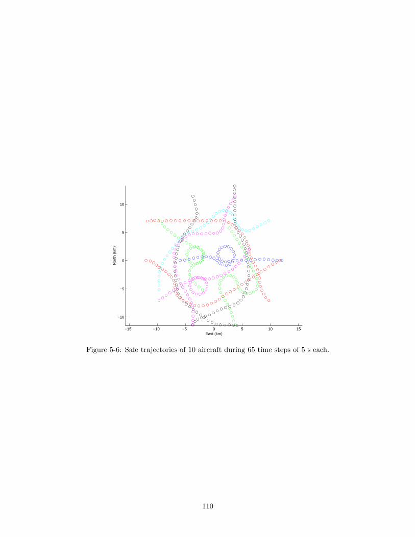
−15 −10 −5 0 5 10 15
−10
−5
0
5
10
East (km)
Nor
th (
km)
Figure 5-6: Safe trajectories of 10 aircraft during 65 time steps of 5 s each.
110
Chapter 6
Multi-Vehicle Path Planning forNon-Line of Sight Communication
This chapter presents a proof-of-concept application of the concepts developed in the previ-ous chapters. We tackle the problem of online connectivity-constrained trajectory planningfor autonomous helicopters through cluttered environments. A lead vehicle must executea certain mission whereby wireless line of sight communication to its ground station islost. Relay helicopters are therefore introduced that must position themselves in such waythat indirect line of sight connectivity between the leader and the ground station is alwaysmaintained. This requires coordinated multi-vehicle trajectory optimization which is tack-led using centralized and distributed receding horizon planning strategies. The problem isagain formulated as a mixed-integer linear program that accounts for the vehicle dynamics,obstacle and collision avoidance, and connectivity constraints. A centralized two-helicoptermission is described for which simulation, hardware in the loop, and actual flight test resultsare presented. Simulation results for distributed scenarios with two and three vehicles aregiven as well.
6.1 Introduction
The problem of interest in this chapter is to guide a small autonomous helicopter through acluttered (e.g. urban) environment in which line of sight communication with a ground sta-tion cannot be maintained due to the presence of obstacles. Depending on the nature of themission, however, some form of communication with the vehicle might be required. For ex-ample, a ground operator may need the capability to upload mission level commands to thehelicopter, such as to fly to and inspect a certain site, and request a real-time video down-link. In addition, he or she should have access to information about the state and health ofthe machine. Practical applications of interest are search and rescue missions, inspectionof disaster sites, urban surveillance, traffic observation, volcanic crater measurements, firefighting unit support, etc.
Depending on the power and antenna characteristics of the wireless transmitter/receiverwith which the helicopter and ground station are equipped, obstruction of the line of sightby nearby buildings or natural obstacles such as hills might significantly degrade the relia-bility and quality of the communication link. Moreover, since the available power on-boardthe vehicle is limited because of battery life (or fuel, in case an alternator is used), the wire-less range will naturally be constrained even in an obstacle-free environment. A reliable
111
communication link between the ground station and the helicopter executing the missioncan then be obtained by introducing a set of relay agents. These can be a combination ofground and aerial vehicles, but we are interested in using only rotorcraft as relay stations:they can take advantage of altitude as an extra degree of freedom, and unlike fixed-wingaircraft, they can hover at a steady location. Indirect communication with the ground sta-tion can then be established by positioning the relay vehicles in such way that a sequenceof direct line of sight links exists between the ground station and the mission helicopter,henceforth called the leader.
As the leader is maneuvering through the environment, the relay helicopters shouldadapt their positions such that visibility/connectivity between the subsequent relay agentsis maintained. A cooperative scheme is therefore required that allows the relay formationto coordinate its reconfiguration with the actions of the leader, and, vice versa, the motionof the leader is constrained by the locations that the relay helicopters can reach. Thiscoordination problem can be formulated as a connectivity-constrained multi-vehicle pathplanning problem, in which feasible trajectories for all agents are computed that optimizea certain cost criterion. Besides maintaining line of sight, feasibility of the trajectories im-plies respecting the helicopters’ kino-dynamic constraints, as well as avoiding obstacles andcollisions. We will focus solely on these dynamic and geometric aspects of the connectivityproblem and ignore mobile networking factors such as fading, cross-talk, and delay, whichcan also affect the availability of links between the vehicles.
Various researchers have approached the problem of motion planning for connectedmulti-agent systems. Nguyen et al. [100] describe the use of mobile relay nodes to extendthe effective range of a ground robot exploring a complex interior environment. The relaynodes follow the lead robot in convoy and automatically stop where needed to form an adhoc network guaranteeing a link between the lead robot and the base station. Variations ofthis algorithm can be found in Sweeney et al. [143]. Another such incremental deploymentstrategy was developed by Howard et al. [50]. These approaches, however, are rule-basedand as such are less flexible than the optimization-based framework presented in this chap-ter. In our methodology, a solution is determined online “from scratch” that accounts forthe features of the particular environment and various constraints on the vehicles. Hybridapproaches in which predetermined navigation or communication recovery behaviors are dy-namically employed online are described in Wagner and Arkin [150], Ulam and Arkin [148],and in Powers and Balch [107]. In the latter, the computational complexity for a planningagent is kept low by assuming that other team members remain in the same position onestep into the future. Our distributed strategy uses a similar idea to maintain feasibility ofthe configuration during the trajectory updates of the planning agent in the relay sequence,more specifically by applying the terminal feasible invariant set principles from Chapters 4and 5.
Next, Beard and McLain [5] use dynamic programming to tackle the problem of search-ing a region of interest using multiple UAVs under communication range and collisionavoidance constraints. Obstacles blocking line of sight between vehicles are not accountedfor, however. Various auction or so-called market-based algorithms have been developed aswell, in which tightly coupled tasks are allocated in a distributed fashion and a solutionis found through a convergence process. Examples include the work of Kalra et al. [59],Lemaire et al. [76] and Bererton et al. [15]. Their focus, however, is on the fair distributionof the tasks and workload among the agents rather than on the actual trajectory planningaccounting for obstacle and collision avoidance. Finally, Spanos and Murray [141] discussthe feasibility aspects of path planning for vehicles connected through a range-constrained
112
wireless network. They define a connectivity robustness measure which quantifies the free-dom of individual vehicles to undergo arbitrary motions without disconnecting the network,but do not explicitly construct feasible trajectories.
Unlike some of the approaches mentioned above, the focus of this chapter is not on the(positioning) task allocation, but on the development of an online cooperative trajectoryplanning algorithm that incorporates connectivity constraints directly into the formulation.In the most general case, different additional constraints can be placed on the individualvehicles: for example, one of the agents may have to remain at ground level, whereas therelay agents must stay above a certain altitude. Our framework will be able to naturallyhandle such requirements. More specifically, we will compute the connectivity-constrainedtrajectories online using MILP again with both centralized and distributed planning strate-gies. This allows us to apply the various concepts and algorithms developed in the previouschapters to a realistic proof-of-concept application and scenario.
6.2 Problem Formulation
6.2.1 Problem Setup
This section extends the basic centralized receding horizon formulation (2.3)-(2.9) for mul-tiple vehicles as presented in Chapter 2 to account for connectivity constraints. Let thevarious agents be denoted by an index i = 0, . . . , L, where i = 0 is the stationary groundstation, i = L indicates the leader, and the remaining index values correspond to the relayhelicopters. The dynamics of the moving vehicles are again characterized by discrete-time,linear state space models (Ai, Bi) with corresponding constraint sets Xi(t) and Ui(t). Theobstacles that are relevant to vehicle i are again represented by the set Oi.
The overall goal of the trajectory planning problem is for the lead vehicle L to perform acertain task while optimizing a particular cost. The leader’s task is again specified as havingto fly to a certain waypoint of interest, denoted as the final state xf ≡ [p′
f v′f ]′, e.g., to
go take video footage at a particular location. As before, a series of task waypoints wouldbe considered as a sequence of independent tasks. Besides maintaining feasibility w.r.t.obstacle and collision avoidance, the motion of the leader will be constrained by the net-work connectivity requirement and the communication capabilities of the relay helicopters.Denote the broadcasting range of each agent i as drelay,i ∈ R. Since we are consideringtwo-directional communication between the vehicles, a communication link between twoagents i and j can only exist if they are within each other’s broadcasting range, or thus ifthe Euclidean distance dij ≡ ‖pi − pj‖ between them is smaller than the shortest range ofthe two: dij ≤ min(drelay,i, drelay,j). Moreover, the visibility between them should not beobstructed. We define these requirements more precisely as follows:
Definition 6.1 (Line of Sight Connection): We say that there exists a line of sightconnection between two agents i and j, positioned respectively at pi and pj, if their Euclideanseparation distance dij = ‖pi−pj‖ is smaller than the shortest broadcasting range of the two,i.e., dij ≤ min(drelay,i, drelay,j), and the line between them does not intersect any obstacles,i.e., pi + λ(pj − pi) /∈ (Oi ∩ Oj), 0 ≤ λ ≤ 1.
In the most general case, the topology of the wireless network could be set up ad hocas part of the optimization problem. In this chapter, however, we consider a fixed order inthe set of relay vehicles i = 1, . . . , L− 1 that corresponds to a linear graph structure: i = 1relays information between i = 0 and i = 2, i = 2 does so between i = 1 and i = 3, and so
113
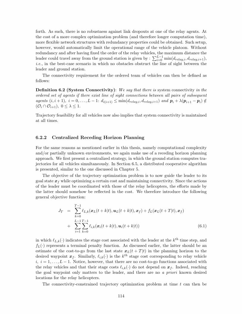
forth. As such, there is no robustness against link dropouts at one of the relay agents. Atthe cost of a more complex optimization problem (and therefore longer computation time),more flexible network structures with redundancy properties could be obtained. Such setup,however, would automatically limit the operational range of the vehicle platoon. Withoutredundancy and after having fixed the order of the relay vehicles, the maximum distance theleader could travel away from the ground station is given by :
∑L−1i=0 min(drelay,i, drelay,i+1),
i.e., in the best-case scenario in which no obstacles obstruct the line of sight between theleader and ground station.
The connectivity requirement for the ordered team of vehicles can then be defined asfollows:
Definition 6.2 (System Connectivity): We say that there is system connectivity in theordered set of agents if there exist line of sight connections between all pairs of subsequentagents (i, i + 1), i = 0, . . . , L − 1: di(i+1) ≤ min(drelay,i, drelay,i+1) and pi + λ(pi+1 − pi) /∈(Oi ∩ Oi+1), 0 ≤ λ ≤ 1.
Trajectory feasibility for all vehicles now also implies that system connectivity is maintainedat all times.
6.2.2 Centralized Receding Horizon Planning
For the same reasons as mentioned earlier in this thesis, namely computational complexityand/or partially unknown environments, we again make use of a receding horizon planningapproach. We first present a centralized strategy, in which the ground station computes tra-jectories for all vehicles simultaneously. In Section 6.5, a distributed cooperative algorithmis presented, similar to the one discussed in Chapter 5.
The objective of the trajectory optimization problem is to now guide the leader to itsgoal state xf while optimizing a certain cost and maintaining connectivity. Since the actionsof the leader must be coordinated with those of the relay helicopters, the efforts made bythe latter should somehow be reflected in the cost. We therefore introduce the followinggeneral objective function:
JT =T−1∑
k=0
ℓL,k(xL(t + k|t), uL(t + k|t), xf ) + fL(xL(t + T |t), xf )
+L−1∑
i=1
T−1∑
k=0
ℓi,k(xi(t + k|t), ui(t + k|t)) (6.1)
in which ℓL,k(·) indicates the stage cost associated with the leader at the kth time step, andfL(·) represents a terminal penalty function. As discussed earlier, the latter should be anestimate of the cost-to-go from the last state xL(t + T |t) in the planning horizon to thedesired waypoint xf . Similarly, ℓi,k(·) is the kth stage cost corresponding to relay vehiclei, i = 1, . . . , L − 1. Notice, however, that there are no cost-to-go functions associated withthe relay vehicles and that their stage costs ℓi,k(·) do not depend on xf . Indeed, reachingthe goal waypoint only matters to the leader, and there are no a priori known desiredlocations for the relay helicopters.
The connectivity-constrained trajectory optimization problem at time t can then be
114
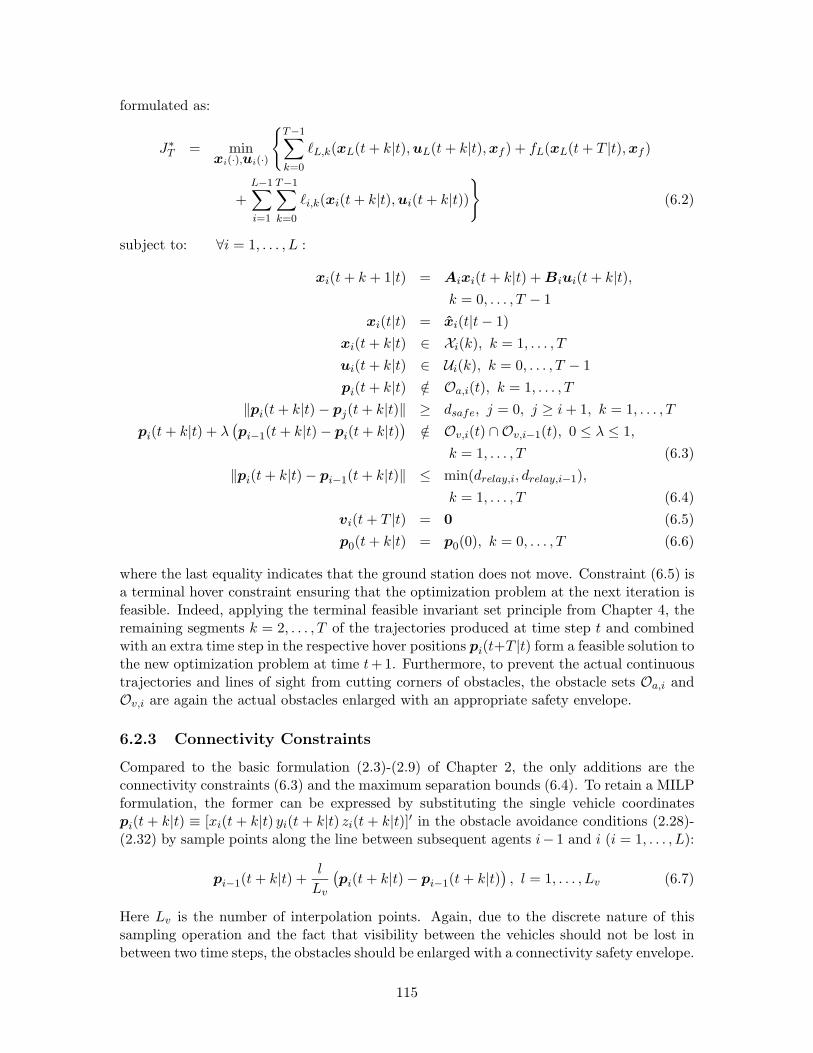
formulated as:
J∗T = min
xi(·),ui(·)
{
T−1∑
k=0
ℓL,k(xL(t + k|t), uL(t + k|t), xf ) + fL(xL(t + T |t), xf )
+L−1∑
i=1
T−1∑
k=0
ℓi,k(xi(t + k|t), ui(t + k|t))}
(6.2)
subject to: ∀i = 1, . . . , L :
xi(t + k + 1|t) = Aixi(t + k|t) + Biui(t + k|t),k = 0, . . . , T − 1
xi(t|t) = xi(t|t − 1)
xi(t + k|t) ∈ Xi(k), k = 1, . . . , T
ui(t + k|t) ∈ Ui(k), k = 0, . . . , T − 1
pi(t + k|t) /∈ Oa,i(t), k = 1, . . . , T
‖pi(t + k|t) − pj(t + k|t)‖ ≥ dsafe, j = 0, j ≥ i + 1, k = 1, . . . , T
pi(t + k|t) + λ(
pi−1(t + k|t) − pi(t + k|t))
/∈ Ov,i(t) ∩ Ov,i−1(t), 0 ≤ λ ≤ 1,
k = 1, . . . , T (6.3)
‖pi(t + k|t) − pi−1(t + k|t)‖ ≤ min(drelay,i, drelay,i−1),
k = 1, . . . , T (6.4)
vi(t + T |t) = 0 (6.5)
p0(t + k|t) = p0(0), k = 0, . . . , T (6.6)
where the last equality indicates that the ground station does not move. Constraint (6.5) isa terminal hover constraint ensuring that the optimization problem at the next iteration isfeasible. Indeed, applying the terminal feasible invariant set principle from Chapter 4, theremaining segments k = 2, . . . , T of the trajectories produced at time step t and combinedwith an extra time step in the respective hover positions pi(t+T |t) form a feasible solution tothe new optimization problem at time t+1. Furthermore, to prevent the actual continuoustrajectories and lines of sight from cutting corners of obstacles, the obstacle sets Oa,i andOv,i are again the actual obstacles enlarged with an appropriate safety envelope.
6.2.3 Connectivity Constraints
Compared to the basic formulation (2.3)-(2.9) of Chapter 2, the only additions are theconnectivity constraints (6.3) and the maximum separation bounds (6.4). To retain a MILPformulation, the former can be expressed by substituting the single vehicle coordinatespi(t + k|t) ≡ [xi(t + k|t) yi(t + k|t) zi(t + k|t)]′ in the obstacle avoidance conditions (2.28)-(2.32) by sample points along the line between subsequent agents i− 1 and i (i = 1, . . . , L):
pi−1(t + k|t) +l
Lv
(
pi(t + k|t) − pi−1(t + k|t))
, l = 1, . . . , Lv (6.7)
Here Lv is the number of interpolation points. Again, due to the discrete nature of thissampling operation and the fact that visibility between the vehicles should not be lost inbetween two time steps, the obstacles should be enlarged with a connectivity safety envelope.
115
The number of sample points should be determined in function of how far the vehicles canbe separated and how large a safety envelope can be tolerated.
Because they are convex, the maximum separation constraints (6.4) are easier to for-mulate and do not require the use of binaries. For simplicity, instead of approximating the2-norm of the separation distance between vehicles i and i− 1 (i = 1, . . . , L) by a collectionof tangent planes, we use an outer 1-norm formulation. Constraints (6.4) then become:
∀k = 1, . . . , T : xi(t + k|t) − xi−1(t + k|t) ≤ min(drelay,i, drelay,i−1)xi−1(t + k|t) − xi(t + k|t) ≤ min(drelay,i, drelay,i−1)
yi(t + k|t) − yi−1(t + k|t) ≤ min(drelay,i, drelay,i−1)yi−1(t + k|t) − yi(t + k|t) ≤ min(drelay,i, drelay,i−1)
zi(t + k|t) − zi−1(t + k|t) ≤ min(drelay,i, drelay,i−1)zi−1(t + k|t) − zi(t + k|t) ≤ min(drelay,i, drelay,i−1)
(6.8)
6.3 Implementation
6.3.1 Helicopter Test-Bed
Using the helicopter model from Chapter 2, the centralized MILP-based receding horizonalgorithm described above was implemented on a testbed consisting of two autonomous X-Cell miniature helicopters, a ground station and a trajectory planning laptop. The X-Cellhelicopters were originally developed at MIT [142, 39] and further improved and commer-cialized by Nascent Technology Corporation (NTC). NTC also extended the original groundstation to support multi-vehicle operations and developed a simulation platform.
Figure 6-1: MIT’s autonomous X-Cell helicopter, equipped with avionics box.
Figure 6-1 shows one of the autonomous X-Cells equipped with its avionics box. Poweris supplied through a 50W alternator that runs off the gas engine and also charges a smartLi-Ion battery that is used as a backup power supply during interrupts. With a full tank,the endurance of the helicopter is 40 minutes. The avionics box contains an Aaeon PC-104computer which runs the QNX real-time operating system. Among other functions, theon-board software features 1) a Kalman filter that combines GPS, IMU, and barometer
116
measurements to estimate the inertial position and velocity, 2) stabilizing control algo-rithms, 3) a waypoint follower, and 4) health management functions. Waypoints can beuploaded from the Windows-based ground station in real-time, and, through file sharing,the downloaded vehicle states are available to the ground-based trajectory planning laptop.
The communication between the ground station and the helicopters is done throughMicrohard Spectra NT920 wireless modems. They operate in the 900 MHz band with a5 miles range, achieve data rates of 276 Kbps, have built-in support for Ethernet, andcan be configured for both “point to multi-point” and relay operation. The latter mode iscritical for beyond-line of sight operations, which is the problem of interest in this chapter.A “heartbeat”-type system monitors the communication link and keeps both the groundstation and the flight computer apprised of its state. If communication is lost, a protocol isset up to re-establish it and continue normal operation, rather than to hang up or otherwisecrash. If communication is lost for longer than a pre-established time out period, however,the helicopter aborts its current mission and automatically returns to the take-off point.This is one of the many autonomy and control augmentation features, which among others,include automatic take-off and landing, transition to hover in case of loss of GPS, andwaypoint following or easy steering by joystick through the ground station laptop.
6.3.2 Mission Scenario
A demonstration mission scenario was developed that is based on military and civilianlaw enforcement requirements for beyond-line of sight urban intelligence, surveillance, andreconnaissance (ISR) operations. The target mission starts with the two helicopters stowedin the back of a ground vehicle (e.g., a truck or SUV). The ground vehicle arrives at an urbansite near an area of interest, the vehicles are unloaded, started, and taken off. This happenssequentially because a single operator guides the take-off process. Since the control systemon the helicopter makes take-off and landing easy, (s)he need not be especially skilled.
The first (mission) helicopter is pull-started, takes off, and is put into hover mode.Next, the second (relay) helicopter is started, takes off, and is put into hover nearby. Bothhelicopters are under control of the ground station at all times. For safety purposes, belowa certain “clearance plane”, they are directly controlled by the operator through joysticksteering. As soon as the vehicles are high enough, they can be guided by point-and-clickoperations on the ground station. Once both helicopters are above the clearance planeand in hover mode, the operator selects a location on the map at which (s)he wants videoinformation. Next, the online trajectory planning software is started and the first seriesof waypoints uploaded to the relay and mission helicopter. The latter then starts flyingtowards the location of interest, thereby avoiding known obstacles and other constraints,while the relay helicopter adjusts its position to maintain line of sight with both the groundstation and the mission helicopter.
An office park in Burlington, MA (where NTC is located), was chosen as the specific testside. Figure 6-2 shows a satellite image of the area, which is about 0.5 km by 0.3 km. Thetake-off area and ground station are located within the rectangle, the circle represents thetarget point for the mission helicopter. There are three large office buildings surroundedby parking lots and wooded areas, next to which are other buildings. A major highway(US 95) runs north-south on the left. The office buildings are about 50 m tall, the treesaround 40 m. Using a combination of GPS measurements and satellite image data fromGoogle Earth [45], a Matlab model of the relevant environment was built which is shownin Figure 6-3. The office buildings were considered separate obstacles, whereas the thick
117
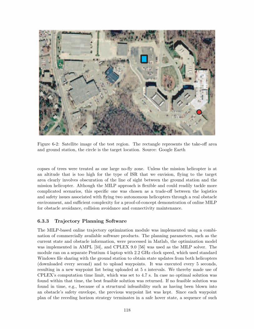
Figure 6-2: Satellite image of the test region. The rectangle represents the take-off areaand ground station, the circle is the target location. Source: Google Earth
copses of trees were treated as one large no-fly zone. Unless the mission helicopter is atan altitude that is too high for the type of ISR that we envision, flying to the targetarea clearly involves obscuration of the line of sight between the ground station and themission helicopter. Although the MILP approach is flexible and could readily tackle morecomplicated scenarios, this specific one was chosen as a trade-off between the logisticsand safety issues associated with flying two autonomous helicopters through a real obstacleenvironment, and sufficient complexity for a proof-of-concept demonstration of online MILPfor obstacle avoidance, collision avoidance and connectivity maintenance.
6.3.3 Trajectory Planning Software
The MILP-based online trajectory optimization module was implemented using a combi-nation of commercially available software products. The planning parameters, such as thecurrent state and obstacle information, were processed in Matlab, the optimization modelwas implemented in AMPL [34], and CPLEX 9.0 [56] was used as the MILP solver. Themodule ran on a separate Pentium 4 laptop with 2.2 GHz clock speed, which used standardWindows file sharing with the ground station to obtain state updates from both helicopters(downloaded every second) and to upload waypoints. It was executed every 5 seconds,resulting in a new waypoint list being uploaded at 5 s intervals. We thereby made use ofCPLEX’s computation time limit, which was set to 4.7 s. In case no optimal solution wasfound within that time, the best feasible solution was returned. If no feasible solution wasfound in time, e.g., because of a structural infeasibility such as having been blown intoan obstacle’s safety envelope, the previous waypoint list was kept. Since each waypointplan of the receding horizon strategy terminates in a safe hover state, a sequence of such
118
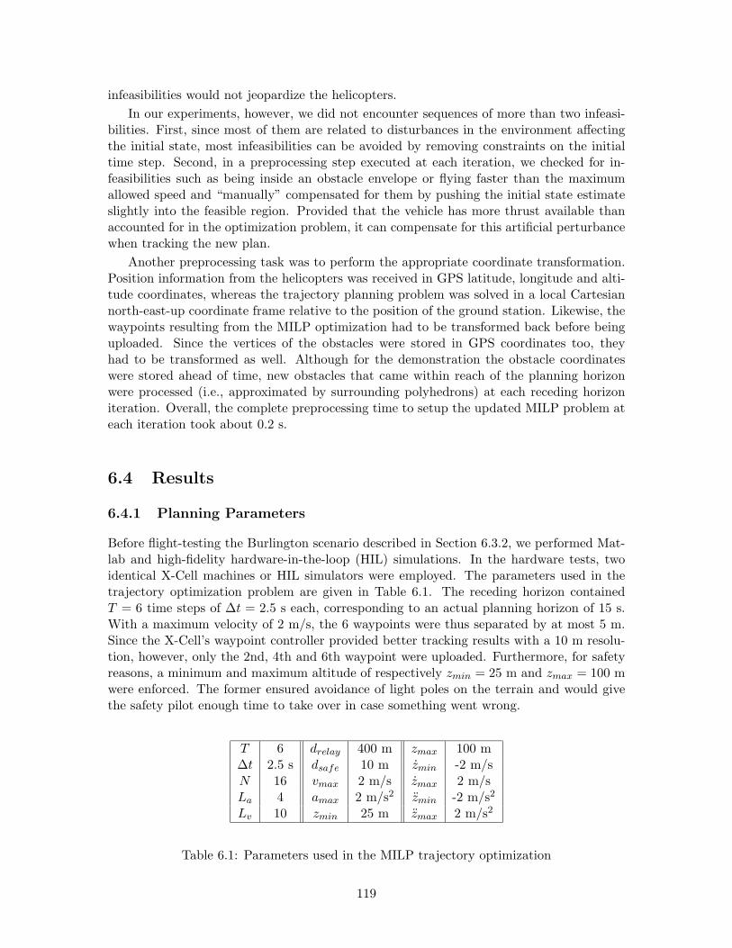
infeasibilities would not jeopardize the helicopters.
In our experiments, however, we did not encounter sequences of more than two infeasi-bilities. First, since most of them are related to disturbances in the environment affectingthe initial state, most infeasibilities can be avoided by removing constraints on the initialtime step. Second, in a preprocessing step executed at each iteration, we checked for in-feasibilities such as being inside an obstacle envelope or flying faster than the maximumallowed speed and “manually” compensated for them by pushing the initial state estimateslightly into the feasible region. Provided that the vehicle has more thrust available thanaccounted for in the optimization problem, it can compensate for this artificial perturbancewhen tracking the new plan.
Another preprocessing task was to perform the appropriate coordinate transformation.Position information from the helicopters was received in GPS latitude, longitude and alti-tude coordinates, whereas the trajectory planning problem was solved in a local Cartesiannorth-east-up coordinate frame relative to the position of the ground station. Likewise, thewaypoints resulting from the MILP optimization had to be transformed back before beinguploaded. Since the vertices of the obstacles were stored in GPS coordinates too, theyhad to be transformed as well. Although for the demonstration the obstacle coordinateswere stored ahead of time, new obstacles that came within reach of the planning horizonwere processed (i.e., approximated by surrounding polyhedrons) at each receding horizoniteration. Overall, the complete preprocessing time to setup the updated MILP problem ateach iteration took about 0.2 s.
6.4 Results
6.4.1 Planning Parameters
Before flight-testing the Burlington scenario described in Section 6.3.2, we performed Mat-lab and high-fidelity hardware-in-the-loop (HIL) simulations. In the hardware tests, twoidentical X-Cell machines or HIL simulators were employed. The parameters used in thetrajectory optimization problem are given in Table 6.1. The receding horizon containedT = 6 time steps of ∆t = 2.5 s each, corresponding to an actual planning horizon of 15 s.With a maximum velocity of 2 m/s, the 6 waypoints were thus separated by at most 5 m.Since the X-Cell’s waypoint controller provided better tracking results with a 10 m resolu-tion, however, only the 2nd, 4th and 6th waypoint were uploaded. Furthermore, for safetyreasons, a minimum and maximum altitude of respectively zmin = 25 m and zmax = 100 mwere enforced. The former ensured avoidance of light poles on the terrain and would givethe safety pilot enough time to take over in case something went wrong.
T 6 drelay 400 m zmax 100 m∆t 2.5 s dsafe 10 m zmin -2 m/sN 16 vmax 2 m/s zmax 2 m/sLa 4 amax 2 m/s2 zmin -2 m/s2
Lv 10 zmin 25 m zmax 2 m/s2
Table 6.1: Parameters used in the MILP trajectory optimization
119
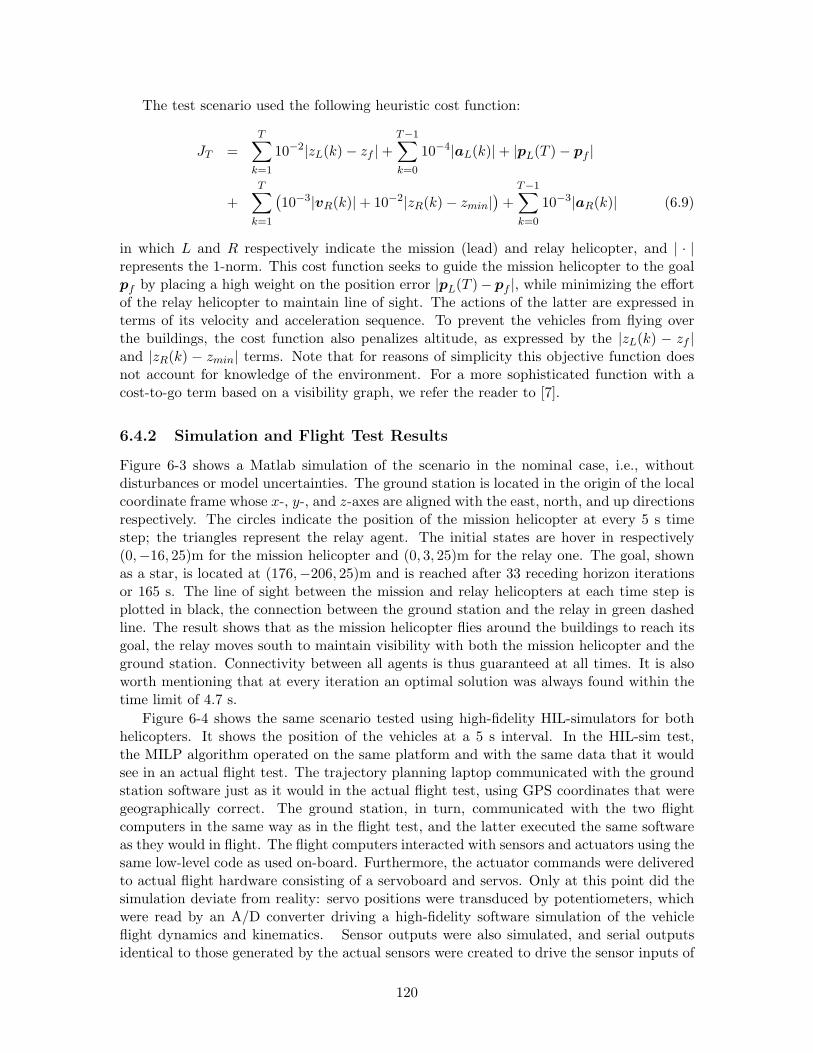
The test scenario used the following heuristic cost function:
JT =T
∑
k=1
10−2|zL(k) − zf | +T−1∑
k=0
10−4|aL(k)| + |pL(T ) − pf |
+T
∑
k=1
(
10−3|vR(k)| + 10−2|zR(k) − zmin|)
+T−1∑
k=0
10−3|aR(k)| (6.9)
in which L and R respectively indicate the mission (lead) and relay helicopter, and | · |represents the 1-norm. This cost function seeks to guide the mission helicopter to the goalpf by placing a high weight on the position error |pL(T )− pf |, while minimizing the effortof the relay helicopter to maintain line of sight. The actions of the latter are expressed interms of its velocity and acceleration sequence. To prevent the vehicles from flying overthe buildings, the cost function also penalizes altitude, as expressed by the |zL(k) − zf |and |zR(k) − zmin| terms. Note that for reasons of simplicity this objective function doesnot account for knowledge of the environment. For a more sophisticated function with acost-to-go term based on a visibility graph, we refer the reader to [7].
6.4.2 Simulation and Flight Test Results
Figure 6-3 shows a Matlab simulation of the scenario in the nominal case, i.e., withoutdisturbances or model uncertainties. The ground station is located in the origin of the localcoordinate frame whose x-, y-, and z-axes are aligned with the east, north, and up directionsrespectively. The circles indicate the position of the mission helicopter at every 5 s timestep; the triangles represent the relay agent. The initial states are hover in respectively(0,−16, 25)m for the mission helicopter and (0, 3, 25)m for the relay one. The goal, shownas a star, is located at (176,−206, 25)m and is reached after 33 receding horizon iterationsor 165 s. The line of sight between the mission and relay helicopters at each time step isplotted in black, the connection between the ground station and the relay in green dashedline. The result shows that as the mission helicopter flies around the buildings to reach itsgoal, the relay moves south to maintain visibility with both the mission helicopter and theground station. Connectivity between all agents is thus guaranteed at all times. It is alsoworth mentioning that at every iteration an optimal solution was always found within thetime limit of 4.7 s.
Figure 6-4 shows the same scenario tested using high-fidelity HIL-simulators for bothhelicopters. It shows the position of the vehicles at a 5 s interval. In the HIL-sim test,the MILP algorithm operated on the same platform and with the same data that it wouldsee in an actual flight test. The trajectory planning laptop communicated with the groundstation software just as it would in the actual flight test, using GPS coordinates that weregeographically correct. The ground station, in turn, communicated with the two flightcomputers in the same way as in the flight test, and the latter executed the same softwareas they would in flight. The flight computers interacted with sensors and actuators using thesame low-level code as used on-board. Furthermore, the actuator commands were deliveredto actual flight hardware consisting of a servoboard and servos. Only at this point did thesimulation deviate from reality: servo positions were transduced by potentiometers, whichwere read by an A/D converter driving a high-fidelity software simulation of the vehicleflight dynamics and kinematics. Sensor outputs were also simulated, and serial outputsidentical to those generated by the actual sensors were created to drive the sensor inputs of
120
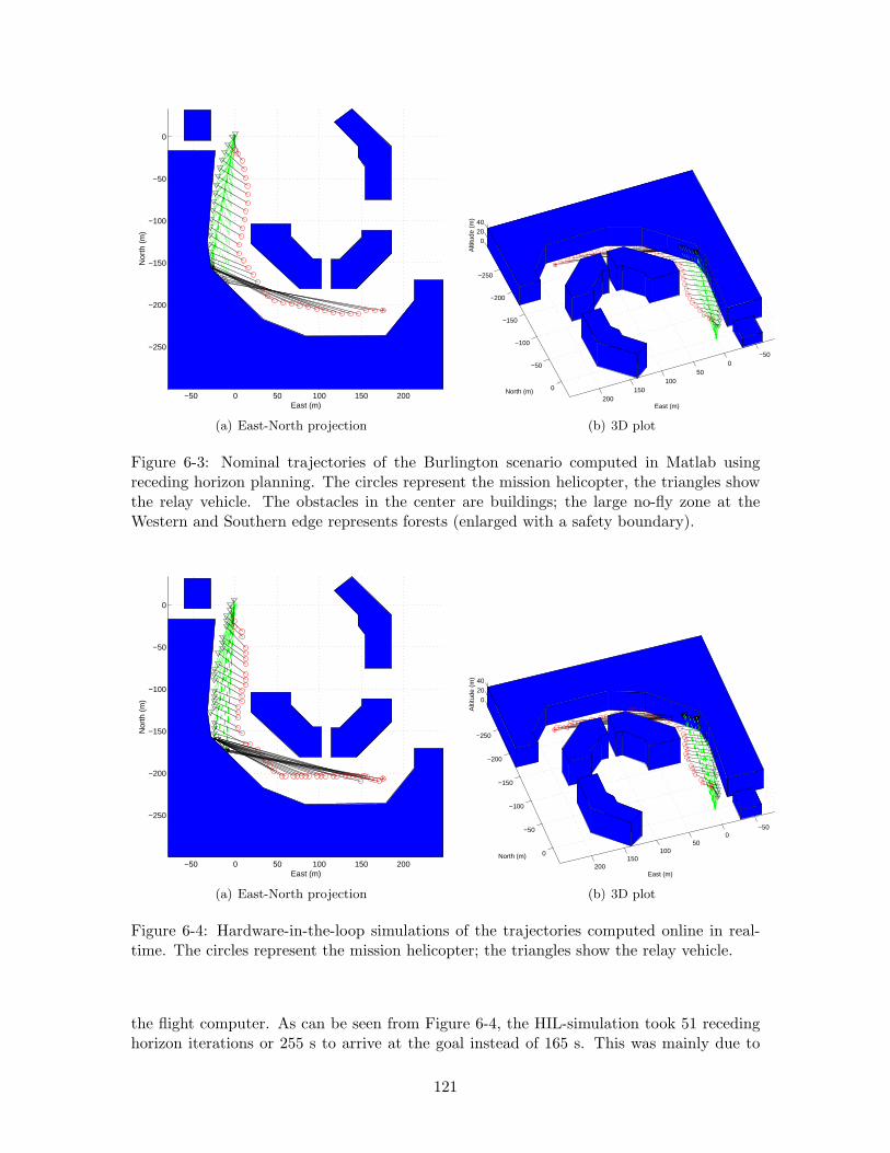
−50 0 50 100 150 200
−250
−200
−150
−100
−50
0
East (m)
Nor
th (
m)
(a) East-North projection
−500
50100
150200
−250
−200
−150
−100
−50
0
02040
East (m)
North (m)
Alti
tude
(m
)
(b) 3D plot
Figure 6-3: Nominal trajectories of the Burlington scenario computed in Matlab usingreceding horizon planning. The circles represent the mission helicopter, the triangles showthe relay vehicle. The obstacles in the center are buildings; the large no-fly zone at theWestern and Southern edge represents forests (enlarged with a safety boundary).
−50 0 50 100 150 200
−250
−200
−150
−100
−50
0
East (m)
Nor
th (
m)
(a) East-North projection
−500
50100
150200
−250
−200
−150
−100
−50
0
0
20
40
East (m)
North (m)
Alti
tude
(m
)
(b) 3D plot
Figure 6-4: Hardware-in-the-loop simulations of the trajectories computed online in real-time. The circles represent the mission helicopter; the triangles show the relay vehicle.
the flight computer. As can be seen from Figure 6-4, the HIL-simulation took 51 recedinghorizon iterations or 255 s to arrive at the goal instead of 165 s. This was mainly due to
121
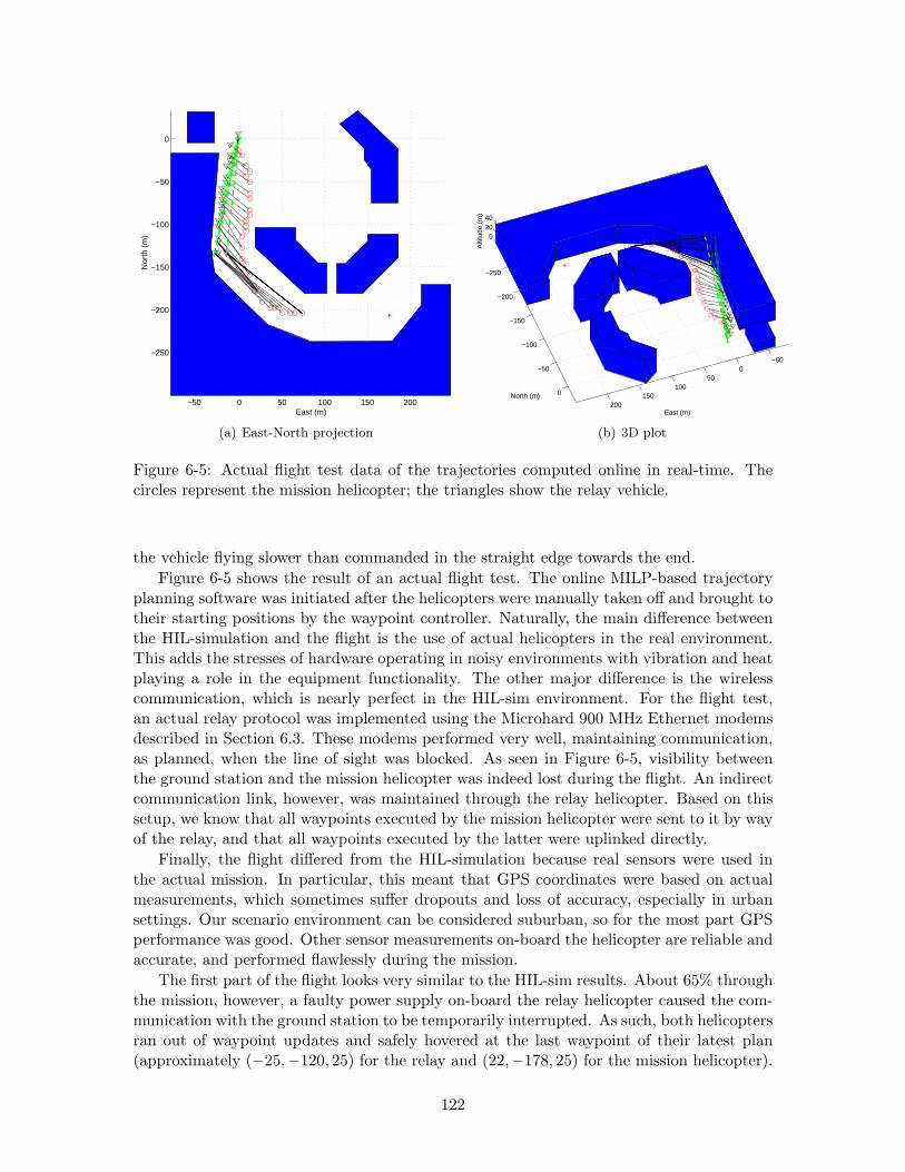
−50 0 50 100 150 200
−250
−200
−150
−100
−50
0
East (m)
Nor
th (
m)
(a) East-North projection
−500
50100
150200
−250
−200
−150
−100
−50
0
02040
East (m)
North (m)
Alti
tude
(m
)
(b) 3D plot
Figure 6-5: Actual flight test data of the trajectories computed online in real-time. Thecircles represent the mission helicopter; the triangles show the relay vehicle.
the vehicle flying slower than commanded in the straight edge towards the end.
Figure 6-5 shows the result of an actual flight test. The online MILP-based trajectoryplanning software was initiated after the helicopters were manually taken off and brought totheir starting positions by the waypoint controller. Naturally, the main difference betweenthe HIL-simulation and the flight is the use of actual helicopters in the real environment.This adds the stresses of hardware operating in noisy environments with vibration and heatplaying a role in the equipment functionality. The other major difference is the wirelesscommunication, which is nearly perfect in the HIL-sim environment. For the flight test,an actual relay protocol was implemented using the Microhard 900 MHz Ethernet modemsdescribed in Section 6.3. These modems performed very well, maintaining communication,as planned, when the line of sight was blocked. As seen in Figure 6-5, visibility betweenthe ground station and the mission helicopter was indeed lost during the flight. An indirectcommunication link, however, was maintained through the relay helicopter. Based on thissetup, we know that all waypoints executed by the mission helicopter were sent to it by wayof the relay, and that all waypoints executed by the latter were uplinked directly.
Finally, the flight differed from the HIL-simulation because real sensors were used inthe actual mission. In particular, this meant that GPS coordinates were based on actualmeasurements, which sometimes suffer dropouts and loss of accuracy, especially in urbansettings. Our scenario environment can be considered suburban, so for the most part GPSperformance was good. Other sensor measurements on-board the helicopter are reliable andaccurate, and performed flawlessly during the mission.
The first part of the flight looks very similar to the HIL-sim results. About 65% throughthe mission, however, a faulty power supply on-board the relay helicopter caused the com-munication with the ground station to be temporarily interrupted. As such, both helicoptersran out of waypoint updates and safely hovered at the last waypoint of their latest plan(approximately (−25,−120, 25) for the relay and (22,−178, 25) for the mission helicopter).
122
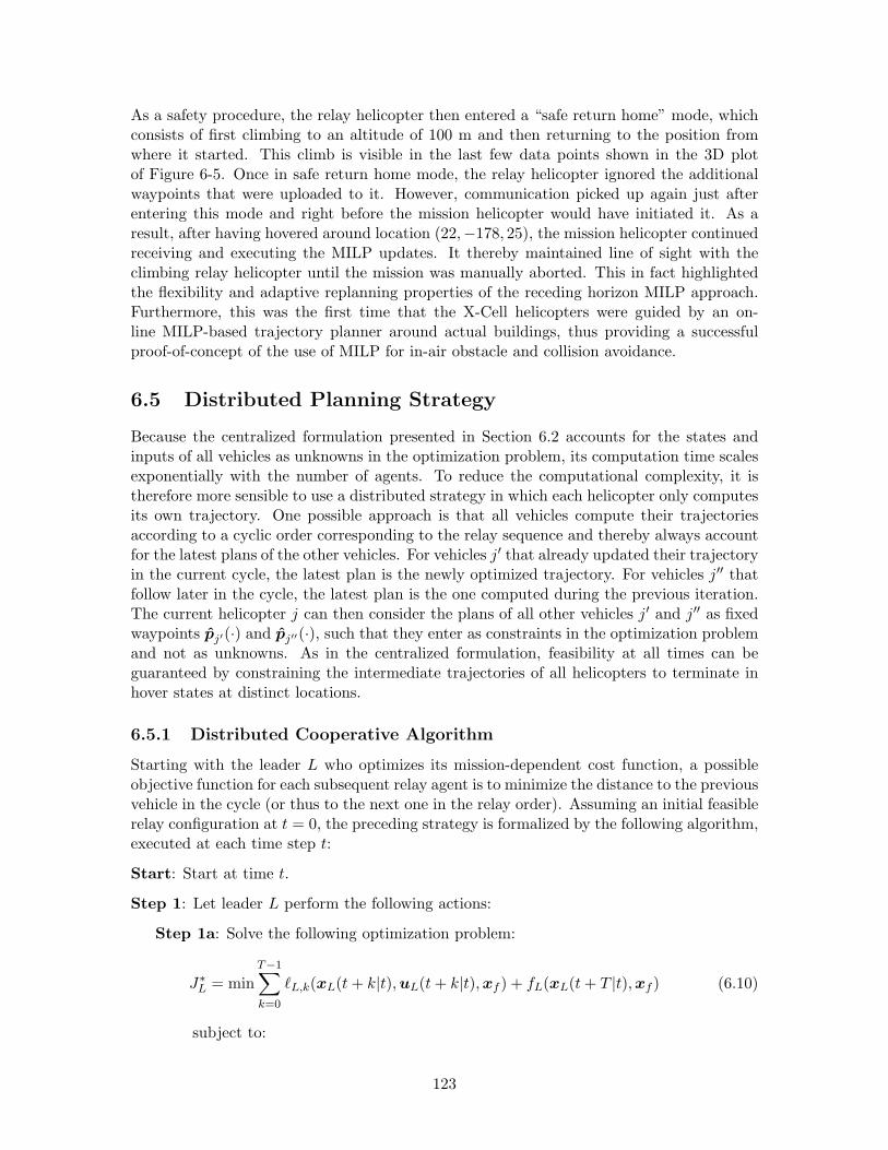
As a safety procedure, the relay helicopter then entered a “safe return home” mode, whichconsists of first climbing to an altitude of 100 m and then returning to the position fromwhere it started. This climb is visible in the last few data points shown in the 3D plotof Figure 6-5. Once in safe return home mode, the relay helicopter ignored the additionalwaypoints that were uploaded to it. However, communication picked up again just afterentering this mode and right before the mission helicopter would have initiated it. As aresult, after having hovered around location (22,−178, 25), the mission helicopter continuedreceiving and executing the MILP updates. It thereby maintained line of sight with theclimbing relay helicopter until the mission was manually aborted. This in fact highlightedthe flexibility and adaptive replanning properties of the receding horizon MILP approach.Furthermore, this was the first time that the X-Cell helicopters were guided by an on-line MILP-based trajectory planner around actual buildings, thus providing a successfulproof-of-concept of the use of MILP for in-air obstacle and collision avoidance.
6.5 Distributed Planning Strategy
Because the centralized formulation presented in Section 6.2 accounts for the states andinputs of all vehicles as unknowns in the optimization problem, its computation time scalesexponentially with the number of agents. To reduce the computational complexity, it istherefore more sensible to use a distributed strategy in which each helicopter only computesits own trajectory. One possible approach is that all vehicles compute their trajectoriesaccording to a cyclic order corresponding to the relay sequence and thereby always accountfor the latest plans of the other vehicles. For vehicles j′ that already updated their trajectoryin the current cycle, the latest plan is the newly optimized trajectory. For vehicles j′′ thatfollow later in the cycle, the latest plan is the one computed during the previous iteration.The current helicopter j can then consider the plans of all other vehicles j′ and j′′ as fixedwaypoints pj′(·) and pj′′(·), such that they enter as constraints in the optimization problemand not as unknowns. As in the centralized formulation, feasibility at all times can beguaranteed by constraining the intermediate trajectories of all helicopters to terminate inhover states at distinct locations.
6.5.1 Distributed Cooperative Algorithm
Starting with the leader L who optimizes its mission-dependent cost function, a possibleobjective function for each subsequent relay agent is to minimize the distance to the previousvehicle in the cycle (or thus to the next one in the relay order). Assuming an initial feasiblerelay configuration at t = 0, the preceding strategy is formalized by the following algorithm,executed at each time step t:
Start: Start at time t.
Step 1: Let leader L perform the following actions:
Step 1a: Solve the following optimization problem:
J∗L = min
T−1∑
k=0
ℓL,k(xL(t + k|t), uL(t + k|t), xf ) + fL(xL(t + T |t), xf ) (6.10)
subject to:
123
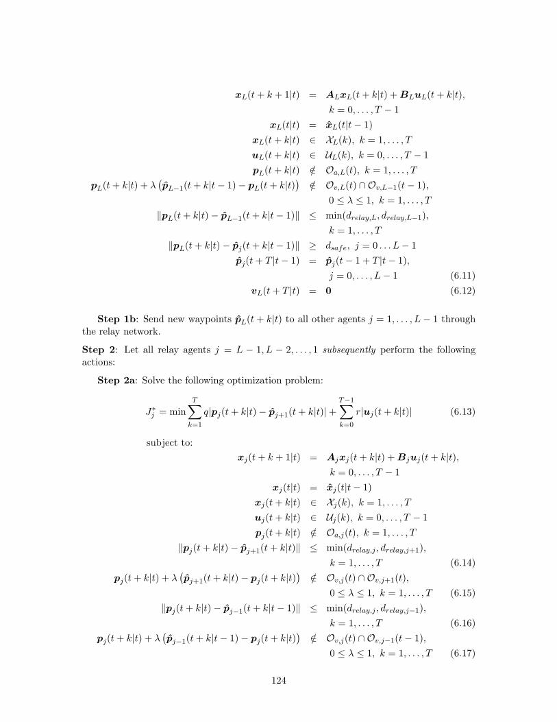
xL(t + k + 1|t) = ALxL(t + k|t) + BLuL(t + k|t),k = 0, . . . , T − 1
xL(t|t) = xL(t|t − 1)
xL(t + k|t) ∈ XL(k), k = 1, . . . , T
uL(t + k|t) ∈ UL(k), k = 0, . . . , T − 1
pL(t + k|t) /∈ Oa,L(t), k = 1, . . . , T
pL(t + k|t) + λ(
pL−1(t + k|t − 1) − pL(t + k|t))
/∈ Ov,L(t) ∩ Ov,L−1(t − 1),
0 ≤ λ ≤ 1, k = 1, . . . , T
‖pL(t + k|t) − pL−1(t + k|t − 1)‖ ≤ min(drelay,L, drelay,L−1),
k = 1, . . . , T
‖pL(t + k|t) − pj(t + k|t − 1)‖ ≥ dsafe, j = 0 . . . L − 1
pj(t + T |t − 1) = pj(t − 1 + T |t − 1),
j = 0, . . . , L − 1 (6.11)
vL(t + T |t) = 0 (6.12)
Step 1b: Send new waypoints pL(t + k|t) to all other agents j = 1, . . . , L − 1 throughthe relay network.
Step 2: Let all relay agents j = L − 1, L − 2, . . . , 1 subsequently perform the followingactions:
Step 2a: Solve the following optimization problem:
J∗j = min
T∑
k=1
q|pj(t + k|t) − pj+1(t + k|t)| +T−1∑
k=0
r|uj(t + k|t)| (6.13)
subject to:
xj(t + k + 1|t) = Ajxj(t + k|t) + Bjuj(t + k|t),k = 0, . . . , T − 1
xj(t|t) = xj(t|t − 1)
xj(t + k|t) ∈ Xj(k), k = 1, . . . , T
uj(t + k|t) ∈ Uj(k), k = 0, . . . , T − 1
pj(t + k|t) /∈ Oa,j(t), k = 1, . . . , T
‖pj(t + k|t) − pj+1(t + k|t)‖ ≤ min(drelay,j , drelay,j+1),
k = 1, . . . , T (6.14)
pj(t + k|t) + λ(
pj+1(t + k|t) − pj(t + k|t))
/∈ Ov,j(t) ∩ Ov,j+1(t),
0 ≤ λ ≤ 1, k = 1, . . . , T (6.15)
‖pj(t + k|t) − pj−1(t + k|t − 1)‖ ≤ min(drelay,j , drelay,j−1),
k = 1, . . . , T (6.16)
pj(t + k|t) + λ(
pj−1(t + k|t − 1) − pj(t + k|t))
/∈ Ov,j(t) ∩ Ov,j−1(t − 1),
0 ≤ λ ≤ 1, k = 1, . . . , T (6.17)
124

‖pj(t + k|t) − pj′(t + k|t)‖ ≥ dsafe, j′ = j + 1, . . . , L (6.18)
‖pj(t + k|t) − pj′′(t + k|t − 1)‖ ≥ dsafe, j′′ = 0, . . . , j − 1 (6.19)
pj′′(t + T |t − 1) = pj′′(t − 1 + T |t − 1),
j′′ = 0, . . . , j − 1 (6.20)
vj(t + T |t) = 0 (6.21)
Step 2b: Send new waypoints pj(t + k|t) to all other agents j′′ = 1, . . . , j − 1 andj′ = j + 1, . . . , L through the relay network.
End: End before time t + 1.
Notice that the cost function (6.10) for the lead vehicle L does not account for the othervehicles and only optimizes a specific mission objective. The cost functions (6.13) for thesubsequent relay agents j, however, seek to minimize the 1-norm distance to the previousagent j + 1 in the decreasing planning sequence, i.e., to the vehicle that just updatedand broadcasted its new waypoints pj+1(t + k|t). Constraints (6.14)-(6.15) express theconnectivity requirement with this previous agent, whereas constraints (6.16)-(6.17) ensureconnectivity with the next agent j − 1 in the update sequence, using the latter’s previouswaypoints pj−1(t + k|t − 1) with an additional time step in the terminal hover locationgiven by equation (6.20). Finally, the collision avoidance constraints (6.18) and (6.19) alsoaccount for the latest waypoint plans of all vehicles in the cycle, namely pj′(t + k|t) foragents j′ = j + 1, . . . , L and pj′′(t + k|t − 1) for agents j′′ = 0, . . . , j − 1.
The planning sequence for all agents j = L, L − 1, . . . , 1 should be completed beforethe next time step. To ensure this, each vehicle in the sequence should be allocated a timeslot in which to compute its trajectory update. An a priori feasible solution will always beavailable, consisting of the remainder of the previous plan with the additional time step inthe terminal hover state. Therefore, if the vehicle cannot find a better solution within theallotted time slot, it can always resort to this backup plan. Constraints (6.11) and (6.20)determine the last time step of this a priori solution for the vehicles following later inthe update cycle. As such, together with the terminal hover constraints (6.12) and (6.21),feasibility of the planning problem for all subsequent agents and time steps is guaranteed.Because it is similar in nature to the feasibility and safety proofs from Chapters 4 and 5, aformal proof of this statement is omitted. It would again consist of the explicit constructionof the feasible solution just described.
6.5.2 Results
Simulation results of the preceding distributed algorithm are shown in Figures 6-6 and 6-7.The former revisits the Burlington scenario with an extra obstacle placed in the field. Tomaintain connectivity with the ground station a second relay vehicle must be introducedwhich, starting from (0, 16, 25)m, positions itself near the lower right corner of the newobstacle. On average, the total cycle for the three vehicles at each receding horizon iterationtook 1.3 s, indicating that the computational complexity of the distributed strategy scalesmuch better with the number of relay agents than the centralized approach.
125
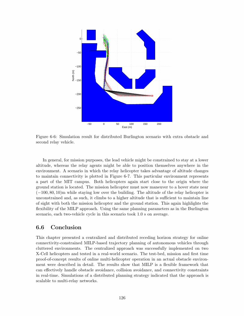
−50 0 50 100 150 200
−250
−200
−150
−100
−50
0
East (m)
Nor
th (
m)
Figure 6-6: Simulation result for distributed Burlington scenario with extra obstacle andsecond relay vehicle.
In general, for mission purposes, the lead vehicle might be constrained to stay at a loweraltitude, whereas the relay agents might be able to position themselves anywhere in theenvironment. A scenario in which the relay helicopter takes advantage of altitude changesto maintain connectivity is plotted in Figure 6-7. This particular environment representsa part of the MIT campus. Both helicopters again start close to the origin where theground station is located. The mission helicopter must now maneuver to a hover state near(−100, 80, 10)m while staying low over the building. The altitude of the relay helicopter isunconstrained and, as such, it climbs to a higher altitude that is sufficient to maintain lineof sight with both the mission helicopter and the ground station. This again highlights theflexibility of the MILP approach. Using the same planning parameters as in the Burlingtonscenario, each two-vehicle cycle in this scenario took 1.0 s on average.
6.6 Conclusion
This chapter presented a centralized and distributed receding horizon strategy for onlineconnectivity-constrained MILP-based trajectory planning of autonomous vehicles throughcluttered environments. The centralized approach was successfully implemented on twoX-Cell helicopters and tested in a real-world scenario. The test-bed, mission and first timeproof-of-concept results of online multi-helicopter operation in an actual obstacle environ-ment were described in detail. The results show that MILP is a flexible framework thatcan effectively handle obstacle avoidance, collision avoidance, and connectivity constraintsin real-time. Simulations of a distributed planning strategy indicated that the approach isscalable to multi-relay networks.
126
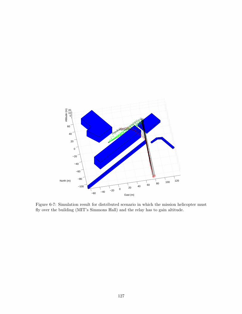
−60 −40 −20 0 20 40 60 80 100 120
−100
−80
−60
−40
−20
0
20
40
60
01020
East (m)
North (m)
Alti
tude
(m
)
Figure 6-7: Simulation result for distributed scenario in which the mission helicopter mustfly over the building (MIT’s Simmons Hall) and the relay has to gain altitude.
127

128
Chapter 7
Implementation of MILP-basedUAV Guidance for Human/UAVTeam
This chapter discusses the implementation of a MILP-based guidance system as part of amanned vehicle – UAV mission system. The overall system enables an operator in a mannedaircraft to issue mission level commands to an autonomous aircraft in real-time. A naturallanguage interface allows the manned and unmanned vehicles to communicate in languagesunderstood by both agents. A task scheduler transforms the commands into a dynamicmission plan consisting of task waypoints. These are then given to the MILP-based trajec-tory optimizer, which safely guides the vehicle through a partially-known environment inreal-time. Integrated simulation and flight-test results are presented that used an F-15 andan autonomous T-33 equipped with Boeing’s UCAV avionics package. These activities werepart of the Capstone Demonstration of the DARPA-sponsored Software Enabled Controleffort. The flight-tests mark the first time that an onboard MILP-based guidance systemwas used to control a UAV. They also mark the first time that a natural language interfacewas used by a manned vehicle to task a UAV in real-time.
7.1 Introduction
Recent advances in guidance and autonomy technology have enabled some UAVs to executesimple mission tasks without human interaction. Most of these tasks are pre-planned usingreconnaissance or environment information. For example, air operations are executed ac-cording to an Air Tasking Order (ATO), which may take up to 72 hours to plan, task andexecute [153]. In volatile situations, however, information about the vehicle’s operating en-vironment may be limited: a detailed map of the environment might not be available aheadof time, and obstacles might be detected while a mission is carried out. In such situations,task planning flexibility and safe trajectory solutions are essential to the survivability andsuccess of the autonomous system: the vehicle’s guidance and mission planning systemsmust possess enough intelligence (and processing power) to recognize and react to changesin the operating conditions.
The complexity of the above problem increases when more than one agent is introduced.For example, if other autonomous agents are added to the mission scenario, then all vehiclesmust resolve information regarding the impending actions of the other vehicles. Similarly,
129
if a manned agent is introduced, the autonomous vehicles must also possess the capabilityto effectively communicate and coordinate their actions with the manned vehicle. Mostunmanned vehicles, however, do not exhibit this level of performance. Intelligent missionand guidance systems providing the flexibility and cooperative behavior needed to completean entire mission autonomously are therefore a topic of active research [67, 122, 25, 47].
This chapter discusses the development, implementation and evaluation of such a systemcontaining a manned vehicle and a UAV operating in a partially-known environment. Itenables the operators of the manned aircraft to issue tasks and mission-level commands tothe unmanned aircraft in real-time using a natural language interface. The latter translatesEnglish sentence commands from the crew to a set of codes understood by the UAV, andvice versa. A task scheduler then transforms these commands into input data of an onlineMILP-based trajectory optimization problem, using the feasible receding horizon planningstrategy from Chapter 4. The overall mission system thus transforms the natural languagecommands of the manned aircraft operators into a mathematical programming problemproducing real-time trajectories that implement the dynamic mission plan of the UAV.
A number of challenges had to be overcome during the development of this system.First, the mechanism allowing both vehicles to communicate with one another needed tobe designed. Second, the UAV guidance technology had to be made robust to changes andthreats in the vehicle’s environment – including changing wind conditions, no-fly zones andother obstacles,– and produce safe trajectories through the partially-known environment.Third, since the system was intended for real-time missions, all developed algorithms neededto reach a solution and resolve any unexpected issues reliably in a pre-defined period of time.
As part of the DARPA-sponsored Software Enabled Control (SEC) Program, the systemwas implemented on a test-bed consisting of an F-15, acting as the manned aircraft, and aT-33 augmented with Boeing’s UCAV avionics package, acting as the autonomous vehicle.During the SEC Capstone Demonstration in June 2004, it was successfully flight-tested atthe NASA Dryden Flight Research Center. These flight-tests mark the first time that anatural language interface was used by a manned vehicle to task a UAV in real-time, andthe first time that a MILP-based guidance system was used to control a UAV.
The chapter is organized as follows. Section 7.2 gives an overview of the SEC experimentand the associated technology development. Section 7.3 describes the natural languageinterface and Section 7.4 covers the task scheduling and communication components. Theimplementation of the real-time trajectory planning software is discussed in Section 7.5.Simulation and flight-test results are presented in Section 7.6.
7.2 Experiment and Technology Overview
7.2.1 Mission Scenario
As originally discussed in [94], as part of the DARPA-sponsored Software Enabled ControlProgram, we were was tasked with developing a mission system and flight-test scenario thatexhibited UAV technology developed at MIT. For this demonstration, two flight assets wereavailable: a Boeing F-15E fighter jet (similar to the aircraft shown in Figure 7-1(a)) anda Lockheed T-33 trainer fighter jet (similar to the one shown in Figure 7-1(b)) that wasequipped with Boeing’s UCAV avionics package. The former was to be flown by a pilot andwill be referred to as the Fixed-Wing (FW) vehicle. The latter was to be guided by ourtechnology and will be referred to as the Unmanned Aerial Vehicle (UAV). Besides these
130
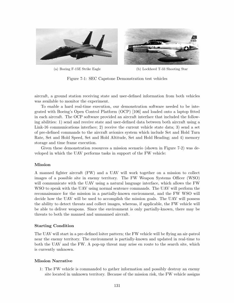
(a) Boeing F-15E Strike Eagle (b) Lockheed T-33 Shooting Star
Figure 7-1: SEC Capstone Demonstration test vehicles
aircraft, a ground station receiving state and user-defined information from both vehicleswas available to monitor the experiment.
To enable a hard real-time execution, our demonstration software needed to be inte-grated with Boeing’s Open Control Platform (OCP) [106] and loaded onto a laptop fittedin each aircraft. The OCP software provided an aircraft interface that included the follow-ing abilities: 1) send and receive state and user-defined data between both aircraft using aLink-16 communications interface; 2) receive the current vehicle state data; 3) send a setof pre-defined commands to the aircraft avionics system which include Set and Hold TurnRate, Set and Hold Speed, Set and Hold Altitude, Set and Hold Heading; and 4) memorystorage and time frame execution.
Given these demonstration resources a mission scenario (shown in Figure 7-2) was de-veloped in which the UAV performs tasks in support of the FW vehicle:
Mission
A manned fighter aircraft (FW) and a UAV will work together on a mission to collectimages of a possible site in enemy territory. The FW Weapon Systems Officer (WSO)will communicate with the UAV using a natural language interface, which allows the FWWSO to speak with the UAV using normal sentence commands. The UAV will perform thereconnaissance for the mission in a partially-known environment, and the FW WSO willdecide how the UAV will be used to accomplish the mission goals. The UAV will possessthe ability to detect threats and collect images, whereas, if applicable, the FW vehicle willbe able to deliver weapons. Since the environment is only partially-known, there may bethreats to both the manned and unmanned aircraft.
Starting Condition
The UAV will start in a pre-defined loiter pattern; the FW vehicle will be flying an air-patrolnear the enemy territory. The environment is partially-known and updated in real-time toboth the UAV and the FW. A pop-up threat may arise en route to the search site, whichis currently unknown.
Mission Narrative
1: The FW vehicle is commanded to gather information and possibly destroy an enemysite located in unknown territory. Because of the mission risk, the FW vehicle assigns
131
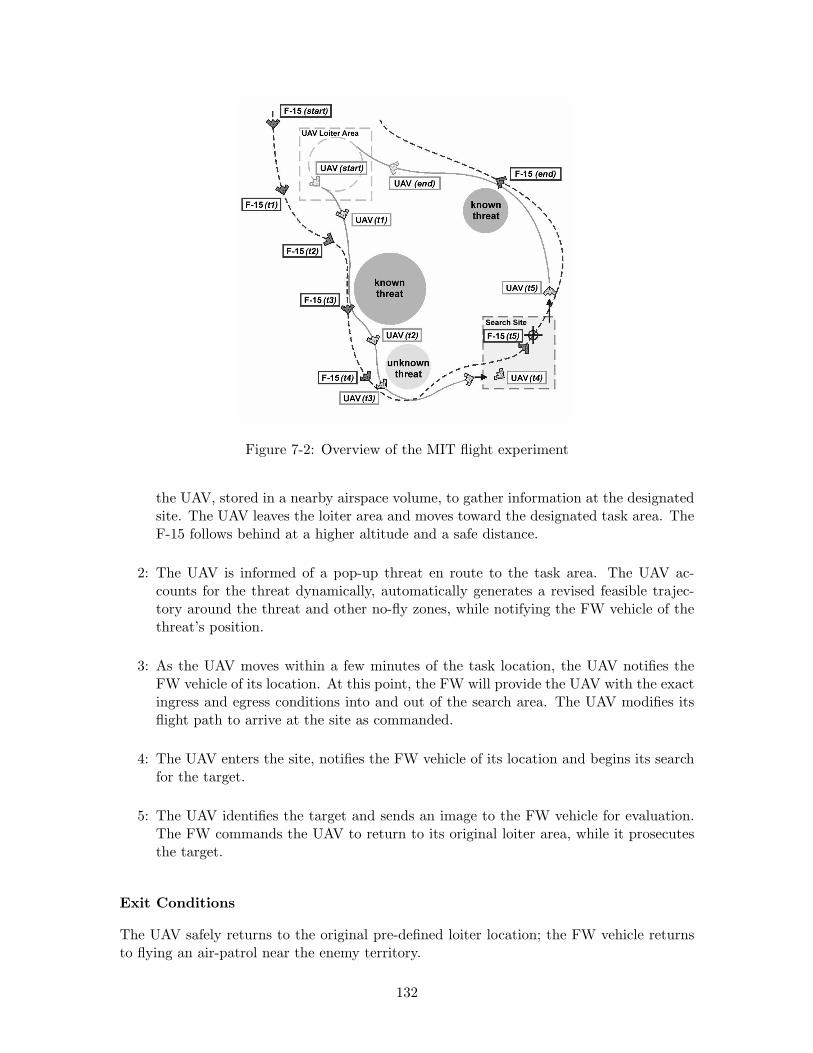
Figure 7-2: Overview of the MIT flight experiment
the UAV, stored in a nearby airspace volume, to gather information at the designatedsite. The UAV leaves the loiter area and moves toward the designated task area. TheF-15 follows behind at a higher altitude and a safe distance.
2: The UAV is informed of a pop-up threat en route to the task area. The UAV ac-counts for the threat dynamically, automatically generates a revised feasible trajec-tory around the threat and other no-fly zones, while notifying the FW vehicle of thethreat’s position.
3: As the UAV moves within a few minutes of the task location, the UAV notifies theFW vehicle of its location. At this point, the FW will provide the UAV with the exactingress and egress conditions into and out of the search area. The UAV modifies itsflight path to arrive at the site as commanded.
4: The UAV enters the site, notifies the FW vehicle of its location and begins its searchfor the target.
5: The UAV identifies the target and sends an image to the FW vehicle for evaluation.The FW commands the UAV to return to its original loiter area, while it prosecutesthe target.
Exit Conditions
The UAV safely returns to the original pre-defined loiter location; the FW vehicle returnsto flying an air-patrol near the enemy territory.
132
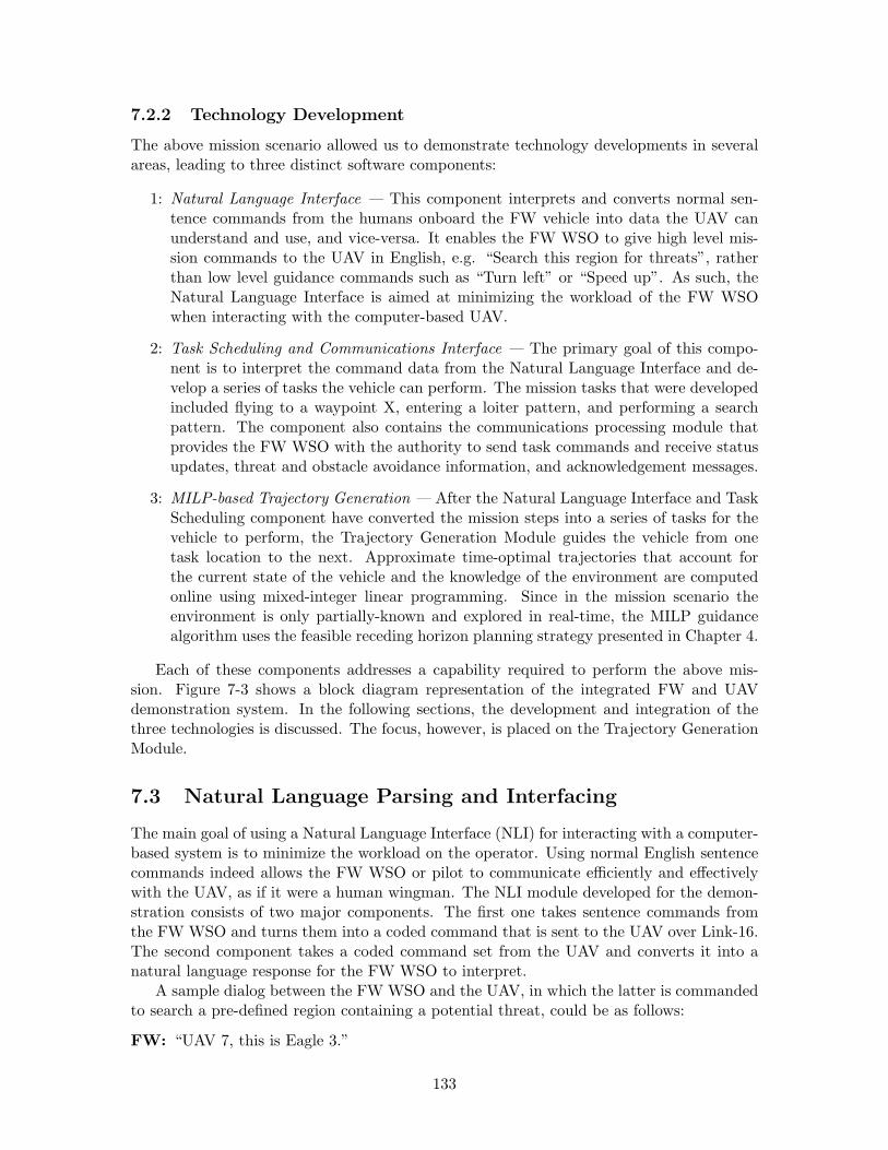
7.2.2 Technology Development
The above mission scenario allowed us to demonstrate technology developments in severalareas, leading to three distinct software components:
1: Natural Language Interface — This component interprets and converts normal sen-tence commands from the humans onboard the FW vehicle into data the UAV canunderstand and use, and vice-versa. It enables the FW WSO to give high level mis-sion commands to the UAV in English, e.g. “Search this region for threats”, ratherthan low level guidance commands such as “Turn left” or “Speed up”. As such, theNatural Language Interface is aimed at minimizing the workload of the FW WSOwhen interacting with the computer-based UAV.
2: Task Scheduling and Communications Interface — The primary goal of this compo-nent is to interpret the command data from the Natural Language Interface and de-velop a series of tasks the vehicle can perform. The mission tasks that were developedincluded flying to a waypoint X, entering a loiter pattern, and performing a searchpattern. The component also contains the communications processing module thatprovides the FW WSO with the authority to send task commands and receive statusupdates, threat and obstacle avoidance information, and acknowledgement messages.
3: MILP-based Trajectory Generation — After the Natural Language Interface and TaskScheduling component have converted the mission steps into a series of tasks for thevehicle to perform, the Trajectory Generation Module guides the vehicle from onetask location to the next. Approximate time-optimal trajectories that account forthe current state of the vehicle and the knowledge of the environment are computedonline using mixed-integer linear programming. Since in the mission scenario theenvironment is only partially-known and explored in real-time, the MILP guidancealgorithm uses the feasible receding horizon planning strategy presented in Chapter 4.
Each of these components addresses a capability required to perform the above mis-sion. Figure 7-3 shows a block diagram representation of the integrated FW and UAVdemonstration system. In the following sections, the development and integration of thethree technologies is discussed. The focus, however, is placed on the Trajectory GenerationModule.
7.3 Natural Language Parsing and Interfacing
The main goal of using a Natural Language Interface (NLI) for interacting with a computer-based system is to minimize the workload on the operator. Using normal English sentencecommands indeed allows the FW WSO or pilot to communicate efficiently and effectivelywith the UAV, as if it were a human wingman. The NLI module developed for the demon-stration consists of two major components. The first one takes sentence commands fromthe FW WSO and turns them into a coded command that is sent to the UAV over Link-16.The second component takes a coded command set from the UAV and converts it into anatural language response for the FW WSO to interpret.
A sample dialog between the FW WSO and the UAV, in which the latter is commandedto search a pre-defined region containing a potential threat, could be as follows:
FW: “UAV 7, this is Eagle 3.”
133
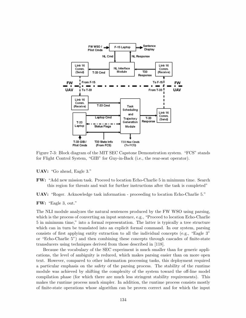
Figure 7-3: Block diagram of the MIT SEC Capstone Demonstration system. “FCS” standsfor Flight Control System, “GIB” for Guy-in-Back (i.e., the rear-seat operator).
UAV: “Go ahead, Eagle 3.”
FW: “Add new mission task. Proceed to location Echo-Charlie 5 in minimum time. Searchthis region for threats and wait for further instructions after the task is completed”
UAV: “Roger. Acknowledge task information - proceeding to location Echo-Charlie 5.”
FW: “Eagle 3, out.”
The NLI module analyzes the natural sentences produced by the FW WSO using parsing,which is the process of converting an input sentence, e.g., “Proceed to location Echo-Charlie5 in minimum time,” into a formal representation. The latter is typically a tree structurewhich can in turn be translated into an explicit formal command. In our system, parsingconsists of first applying entity extraction to all the individual concepts (e.g., “Eagle 3”or “Echo-Charlie 5”) and then combining these concepts through cascades of finite-statetransducers using techniques derived from those described in [118].
Because the vocabulary of the SEC experiment is much smaller than for generic appli-cations, the level of ambiguity is reduced, which makes parsing easier than on more opentext. However, compared to other information processing tasks, this deployment requireda particular emphasis on the safety of the parsing process. The stability of the runtimemodule was achieved by shifting the complexity of the system toward the off-line modelcompilation phase (for which there are much less stringent stability requirements). Thismakes the runtime process much simpler. In addition, the runtime process consists mostlyof finite-state operations whose algorithm can be proven correct and for which the input
134
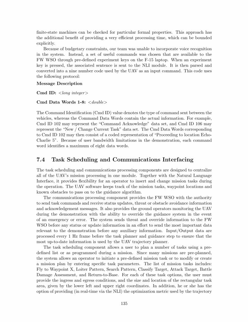
finite-state machines can be checked for particular formal properties. This approach hasthe additional benefit of providing a very efficient processing time, which can be boundedexplicitly.
Because of budgetary constraints, our team was unable to incorporate voice recognitionin the system. Instead, a set of useful commands was chosen that are available to theFW WSO through pre-defined experiment keys on the F-15 laptop. When an experimentkey is pressed, the associated sentence is sent to the NLI module. It is then parsed andconverted into a nine number code used by the UAV as an input command. This code usesthe following protocol:
Message Description
Cmd ID: <long integer>
Cmd Data Words 1-8: <double>
The Command Identification (Cmd ID) value denotes the type of command sent between thevehicles, whereas the Command Data Words contain the actual information. For example,Cmd ID 102 may represent the “Command Acknowledge” data set, and Cmd ID 106 mayrepresent the “New / Change Current Task” data set. The Cmd Data Words correspondingto Cmd ID 102 may then consist of a coded representation of “Proceeding to location Echo-Charlie 5”. Because of user bandwidth limitations in the demonstration, each commandword identifies a maximum of eight data words.
7.4 Task Scheduling and Communications Interfacing
The task scheduling and communications processing components are designed to centralizeall of the UAV’s mission processing in one module. Together with the Natural LanguageInterface, it provides flexibility for an operator to insert and change mission tasks duringthe operation. The UAV software keeps track of the mission tasks, waypoint locations andknown obstacles to pass on to the guidance algorithm.
The communications processing component provides the FW WSO with the authorityto send task commands and receive status updates, threat or obstacle avoidance informationand acknowledgement messages. It also provides the ground operators monitoring the UAVduring the demonstration with the ability to override the guidance system in the eventof an emergency or error. The system sends threat and override information to the FWWSO before any status or update information in an effort to send the most important datarelevant to the demonstration before any auxiliary information. Input/Output data areprocessed every 1 Hz frame before the task planner and guidance step to ensure that themost up-to-date information is used by the UAV trajectory planner.
The task scheduling component allows a user to plan a number of tasks using a pre-defined list or as programmed during a mission. Since many missions are pre-planned,the system allows an operator to initiate a pre-defined mission task or to modify or createa mission plan by entering specific task parameters. The list of mission tasks includes:Fly to Waypoint X, Loiter Pattern, Search Pattern, Classify Target, Attack Target, BattleDamage Assessment, and Return-to-Base. For each of these task options, the user mustprovide the ingress and egress conditions, and the size and location of the rectangular taskarea, given by the lower left and upper right coordinates. In addition, he or she has theoption of providing (in real-time via the NLI) the optimization metric used by the trajectory
135
generation algorithm (i.e., minimum time, minimum fuel, or the amount of time to finishthe task).
Next, the operator can either give the vehicle a new task or change the current task itis performing. A “New Task” command is added to the end of the UAV task list and isexecuted after all of the tasks currently in the scheduler have been completed. A “ChangeTask” command, on the other hand, modifies the current task performed by the UAV.Once a task is completed, it is removed from the list. After each of these actions, anacknowledgement is sent to the FW WSO and the updated task information is included inthe data sent to the Trajectory Generation Module.
To reduce the complexity of the demonstration system, only the current task could bemodified, although future versions of this system will have the capability to change any of thetasks in the scheduler. Furthermore, because of communication link bandwidth constraints,the FW WSO did not have the capability to define a new task or adjust parameters in thecurrent task manually. Instead, he was able to command the vehicle to perform tasks froma pre-defined library using the experiment keys on the FW laptop.
7.5 MILP-based Trajectory Generation Module
After the Natural Language Interface and Task Scheduling components have converted themission steps into a series of tasks for the UAV to perform, the Trajectory Generation Mod-ule guides the vehicle from one task location to the next, i.e., from an initial state to a desiredone, through an obstacle field while optimizing a certain objective. For the demonstration,2D scenarios were considered in which no-fly zones or “obstacles” are detected while themission is carried out, but such that the environment is always fully characterized insidea certain detection region around the aircraft. The demonstration scenarios used a circu-lar region of radius 9 mi and assumed that all obstacles O within that radius were static.The formulation could, however, be easily generalized to account for any detection shape,such as a radar cone, and for unknown areas within that shape. Since the environmentis only partially-known and further explored in real-time, a feasible receding horizon plan-ning strategy is implemented using left and right turning loiter circles as terminal feasibleinvariant sets.
7.5.1 MILP Formulation
Dynamic Model
System identification experiments using the UAV DemoSim simulation software providedby Boeing gave us insight into the velocity response of the UAV. A piecewise linear first-order approximation was deemed to be sufficient for guidance purposes. The time constantand DC gain of the transfer function were identified for a discrete set of forward velocities(from 350 fps to 500 fps with a resolution of 10 fps) and stored in a look-up table. Ateach iteration of the receding horizon strategy, the model corresponding to the velocity atthat time step was used, thus linearizing the nonlinear response into several LTI modesscheduled around the initial velocity.
Taking the desired planar inertial velocity as input then gives the continuous-time statespace model:
x(t) = − 1τl
x(t) + kl
τlxcmd(t)
y(t) = − 1τl
y(t) + kl
τlycmd(t)
(7.1)
136
where τl is the time constant and kl is the gain corresponding to the lth LTI mode. Asin equation (5.3), it was discretized using the bilinear transform. Since the typical timeconstant of the T-33 velocity response was around 9.7 s, a time step of ∆t = 10 s wasused. With additional constraints on speed and acceleration, this model produced goodresults for tasks requiring intensive waypoint tracking and sharp turns (i.e., the loiter andsearch tasks). For less aggressive trajectories with more or less constant speed, such aswhen transitioning between two task areas, the simpler (2D) double integrator model (2.20)was used that does not distinguish between the different LTI modes.
As discussed in Chapter 2, since it takes a certain time to compute the trajectory, theinitial state x(0) should be an estimate of the vehicle’s state when the plan is actuallyimplemented. In our case, the computation delay was approximately 1 s. In addition, a1.2 s actuator delay had to be accounted for. To obtain an estimate of the initial state atthe next iteration, the dynamics were thus propagated forward according to the previousplan for 2.2 s.
To ensure that the planned trajectory respected the velocity limits of the vehicle, thesame maximum and minimum speed constraints were included as in inequalities (2.21)and (2.23)-(2.25). For the reference velocity model (7.1) these were formulated in termsof the velocity commands xcmd(k) and ycmd(k), for the double integrator model in termsof the state velocity variables x(k) and y(k). The minimum and maximum bounds wererespectively set to vmin = 400 fps and vmax = 450 fps, using a polygonal approximationwith N = 32. To avoid infeasible problems in the event the actual ground speed fell outsidethese bounds (e.g., because of wind gusts), their values were accordingly adapted online.
Since the dynamics are homogeneous in the x- and y-coordinates and as such ignoredifferences in the lateral and longitudinal aircraft dynamics, we added constraints capturinglimits on turn rate and on forward and lateral acceleration. When flying at a relativelyconstant speed, the following acceleration constraints were sufficient:
∀k ∈ [0, . . . , T − 1], ∀n ∈ [1, . . . , N ] :
x(k) sin(2πn/N) + y(k) cos(2πn/N) ≤ alat (7.2)
for the double integrator model, and
∀k ∈ [1, . . . , T − 1], ∀n ∈ [1, . . . , N ] :
(xcmd(k) − xcmd(k − 1)) sin(2πn/N)
+ (xcmd(k) − xcmd(k − 1)) cos(2πn/N) ≤ alat∆t (7.3)
for the reference velocity model. The lateral acceleration bound was set at alat = 18.1 ft2/s,corresponding to a maximum turn rate of ωmax = alat/vmin = 2.6 deg/s at vmin = 400 fps.
When the velocity is allowed to change, however, these inequalities overestimate theavailable forward acceleration, which was limited to afwd = 5.0 ft2/s. Therefore, to dis-tinguish between forward and lateral acceleration, the following constraints were included,similar to inequalities (2.22-b):
∀k ∈ [0 . . . T − 1], ∀n ∈ [1 . . . N ] :
(x(k) + αv(0)−1y(k)) sin(2πn/N) + (y(k) − αv(0)−1x(k)) cos(2πn/N) ≤ β (7.4)
(x(k) − αv(0)−1y(k)) sin(2πn/N) + (y(k) + αv(0)−1x(k)) cos(2πn/N) ≤ β (7.5)
for the double integrator model, and
137
∀k ∈ [1, . . . , T − 1], ∀n ∈ [1, . . . , N ] :
(xcmd(k) − xcmd(k − 1) + αv(0)−1y(k)∆t) sin(2πn/N)
+ (ycmd(k) − ycmd(k − 1) − αv(0)−1x(k)∆t) cos(2πn/N) ≤ β∆t (7.6)
(xcmd(k) − xcmd(k − 1) − αv(0)−1y(k)∆t) sin(2πn/N)
+ (ycmd(k) − ycmd(k − 1) + αv(0)−1x(k)∆t) cos(2πn/N) ≤ β∆t (7.7)
for the reference velocity model. Here, v(0) is the current absolute ground speed, α =
(a2lat − a2
fwd)/(2afwd) = 30.4 fps2/s, and β =√
α2 + a2lat = 35.4 fps2/s. As discussed in
Section 3.4, these inequalities describe the intersection of two circles in which the inertialacceleration vector must lie. The short axis of this intersection has length 2afwd and isaligned with the velocity vector at the first time step. The long axis captures the largerlateral acceleration bound and has length 2alat. As such, the intersection approximates thedynamically feasible acceleration profile at the initial time step.
Feasibility Constraints
The demonstration only considered rectangular no-fly zones aligned with the east-northcoordinate frame, using constraints (2.30) in 2D to guarantee obstacle avoidance. To preventthe UAV from cutting corners, the actual obstacles were enlarged with a safety boundaryof dsafe = vmax∆t/
√2 ≈ 3200 ft. Feasibility was guaranteed by ensuring that either a left
or right loiter circle lying inside the circular detection region did not intersect with any ofthe obstacles. As detailed by inequalities (5.9)-(5.10), sample points along both circles wereexpressed as affine functions of the last state x(T ) in the planning horizon. Again, becauseof the sampling procedure, the obstacles were enlarged on all sides by a thickness dloiter.The demonstration used 8 sample points, which, given a maximum turn radius of 1.9 mi,resulted in dloiter = 0.6 mi.
Cost Function
The objective was to guide the UAV between waypoints in the fastest possible way. Theexact shortest time between two states, however, can only be computed if the planninghorizon spans that arrival time, or if an exact cost-to-go is known. Since in the scenario ofinterest the environment was not characterized beyond a certain detection radius aroundthe vehicle, computing an exact time-to-go function as proposed in [7] and [68] was notpossible. Instead, the following heuristic was used.
If there are no known obstacles intersecting the straight line between the waypoint andthe current location, that waypoint is used as the desired state in the cost function. Incase there are obstacles blocking this direct line of sight, the shortest path (as far as theknown obstacles are concerned) must go through one of the visible corner points of theseno-fly zones. This point can then act as an intermediate waypoint en route to the finaldestination. To determine this optimal intermediate point, a grid is constructed betweenthe corner points of all known obstacles interfering with the line of sight. A shortest pathalgorithm is then run to compute the approximate shortest time towards the goal fromeach visible corner point, thereby assuming that the UAV is flying at maximum speed. Assuch, the “best” intermediate waypoint is determined by minimizing the total time fromthe current location to one of the visible vertices and from that vertex to the destinationas given by the approximate cost-to-go function.
138
Using this intermediate (or, in the obstacle-free case, the original) waypoint pf =[xf yf ]′, the piecewise linear cost function
minJ =
T∑
k=0
−qv(k)′(pf − pestim) + r|p(k) − pf | (7.8)
was used to design a fast trajectory between the initial position p(0) = pestim = [x(0) y(0)]′
in the planning horizon and pf . Similarly to cost functions (3.35) and (5.12), the firstterm in this objective function tries to maximize the scalar product of the inertial velocityv(k) = [x(k) y(k)]′ with the vector that is pointing from the initial position to the desiredone, speeding the aircraft up to its maximal velocity and turning it towards waypoint pf .
If, at a certain iteration, the planned trajectory passes through or near waypoint pf ata time step Tf ≤ T in the planning horizon, the cost function for the next iteration is splitinto two parts:
min J =
Tf−1∑
k=0
−qfv(k)′(pf − pestim) + rf |p(k) − pf |
+
T∑
k=Tf
−qnv(k)′(pn − pf ) + rn|p(k) − pn| (7.9)
in which pn is the next (intermediate) waypoint. The first Tf − 1 time steps are thus usedto minimize the cost towards waypoint pf ; the remaining steps aim at minimizing the costtowards the next waypoint pn. As a result, depending on the relative weighting, the MILPoptimization will produce a trajectory that passes through or close by pf and aims for pn
next. The SEC demonstration used T = 6, corresponding to an effective planning length of1 minute, and all weights in (7.8) and (7.9) were set to 1.
7.5.2 Implementation
The Trajectory Generation Module was implemented in C++ and ILOG’s Concert Tech-nologies. To interface with the UAV avionics and guarantee hard real-time execution, itwas integrated with Boeing’s Open Control Platform (OCP) [106]. The software ran on aPentium 4 Linux laptop with 2.4 GHz clock speed that was mounted in the aircraft, andinteracted with the UAV avionics through a set of pre-defined command variables. Throughthe OCP interface the laptop received GPS, ground speed and turn rate data, among other,at a rate of 20 Hz. The guidance module itself, however, only ran at 1 Hz. It consisted ofthree subroutines: a pre-processing step, an optimization step, and a post-processing step,which are now discussed in more detail.
Pre-Processing
The pre-processing routine was called every second and determined all parameters of theMILP problem. It subsequently 1) selected the correct LTI model, 2) estimated the initialstate for the current planning horizon, 3) determined the relevant obstacles, 4) enlarged theobstacles with the appropriate safety envelope, 5) determined the intermediate waypoint,and 6) selected the appropriate cost function. In addition, for numerical stability purposesand to speed up the MILP optimization, all latitude/longitude position data and obstacle
139

coordinates were transformed to an east-north axis frame in kilometer units with the currentposition of the aircraft as the origin. The ground velocity of the aircraft was scaled to km/saccordingly.
Optimization
The optimization step was implemented using the ILOGs Concert Technologies, a C++based modeling language for use with CPLEX. It enables one to encode a large MILPproblem in a compact form that is similar to the mathematical representation of it. Toguarantee hard real-time execution of the mission software, we again used CPLEX’s optionallimit on computation time, which was set to 0.85 s. After the allocated time has passed,CPLEX then either returns a feasible solution within a predefined optimality gap (set to10−4), a feasible solution outside the optimality gap, or no solution at all. The last situationoccurs when the MILP itself is infeasible or when no feasible solution can be found in time(e.g., because the problem is too complex).
Ideally, by definition of the loiter circle constraints, the trajectory planning problemremains feasible at all times. However, because of disturbances such as wind gusts, theinitial velocity might fall outside the constraint bounds or the vehicle might be blown offcourse to a position from where an obstacle-free MILP solution no longer exists. Thefirst situation is easy to spot and can be resolved ahead of time by resetting the velocitybounds in the pre-processing step. Infeasibilities caused by obstacles, however, are harderto predict and resolve. In that case, the UAV should resort to its backup plan, consistingof the remaining time steps and loiter circle of the previous plan.
If the control authority used in the MILP problem (i.e., the admissible accelerationand turn rate limit) is somewhat conservative w.r.t. the actual performance of the vehicle,robust trajectories can be designed. Then, in case the UAV gets blown off course to astate from which no feasible solution to the MILP exists, the aircraft can use its additionalcontrol authority to get back to feasibility within a few time steps [71]. Our code thereforeused maximum acceleration and turn rate bounds that are smaller than the actual onesavailable to the waypoint controller. As a result, sequences of more than two infeasiblereceding horizon iterations never occurred.
Although the pre-processing step was repeated every second, the optimization functionwas nominally only executed every 10 s: the ∼10 s time constant of the T-33 made a higherplanning rate unnecessary. Only when a large disturbance or an additional obstacle wasdetected, or when the vehicle was in backup plan mode (i.e., when the last MILP problemwas infeasible), was the optimization routine executed at the next second. This way theavailable time slots could be occupied by computations required by the Task Schedulingand Natural Language Interface components.
Post-Processing
The post-processing routine performed the feasibility check by interpreting a CPLEX flagand updated the current trajectory (i.e., the current waypoint list), the loiter direction anda backup plan waypoint counter accordingly. In the nominal case where a feasible solutionwas found, the variables of interest were the 6 new states of the planning horizon (i.e., thenew waypoint coordinates with corresponding velocity vectors) and the new loiter direction.The coordinates were first transformed back to the original Greenwich-referenced longitudeand latitude axis frame and the velocity was rescaled to fps. Next, the old plan was flushed
140
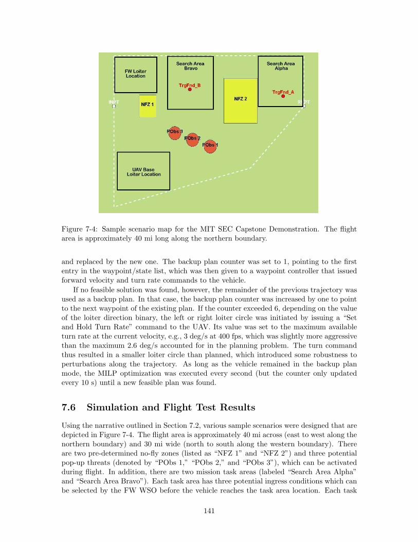
Figure 7-4: Sample scenario map for the MIT SEC Capstone Demonstration. The flightarea is approximately 40 mi long along the northern boundary.
and replaced by the new one. The backup plan counter was set to 1, pointing to the firstentry in the waypoint/state list, which was then given to a waypoint controller that issuedforward velocity and turn rate commands to the vehicle.
If no feasible solution was found, however, the remainder of the previous trajectory wasused as a backup plan. In that case, the backup plan counter was increased by one to pointto the next waypoint of the existing plan. If the counter exceeded 6, depending on the valueof the loiter direction binary, the left or right loiter circle was initiated by issuing a “Setand Hold Turn Rate” command to the UAV. Its value was set to the maximum availableturn rate at the current velocity, e.g., 3 deg/s at 400 fps, which was slightly more aggressivethan the maximum 2.6 deg/s accounted for in the planning problem. The turn commandthus resulted in a smaller loiter circle than planned, which introduced some robustness toperturbations along the trajectory. As long as the vehicle remained in the backup planmode, the MILP optimization was executed every second (but the counter only updatedevery 10 s) until a new feasible plan was found.
7.6 Simulation and Flight Test Results
Using the narrative outlined in Section 7.2, various sample scenarios were designed that aredepicted in Figure 7-4. The flight area is approximately 40 mi across (east to west along thenorthern boundary) and 30 mi wide (north to south along the western boundary). Thereare two pre-determined no-fly zones (listed as “NFZ 1” and “NFZ 2”) and three potentialpop-up threats (denoted by “PObs 1,” “PObs 2,” and “PObs 3”), which can be activatedduring flight. In addition, there are two mission task areas (labeled “Search Area Alpha”and “Search Area Bravo”). Each task area has three potential ingress conditions which canbe selected by the FW WSO before the vehicle reaches the task area location. Each task
141
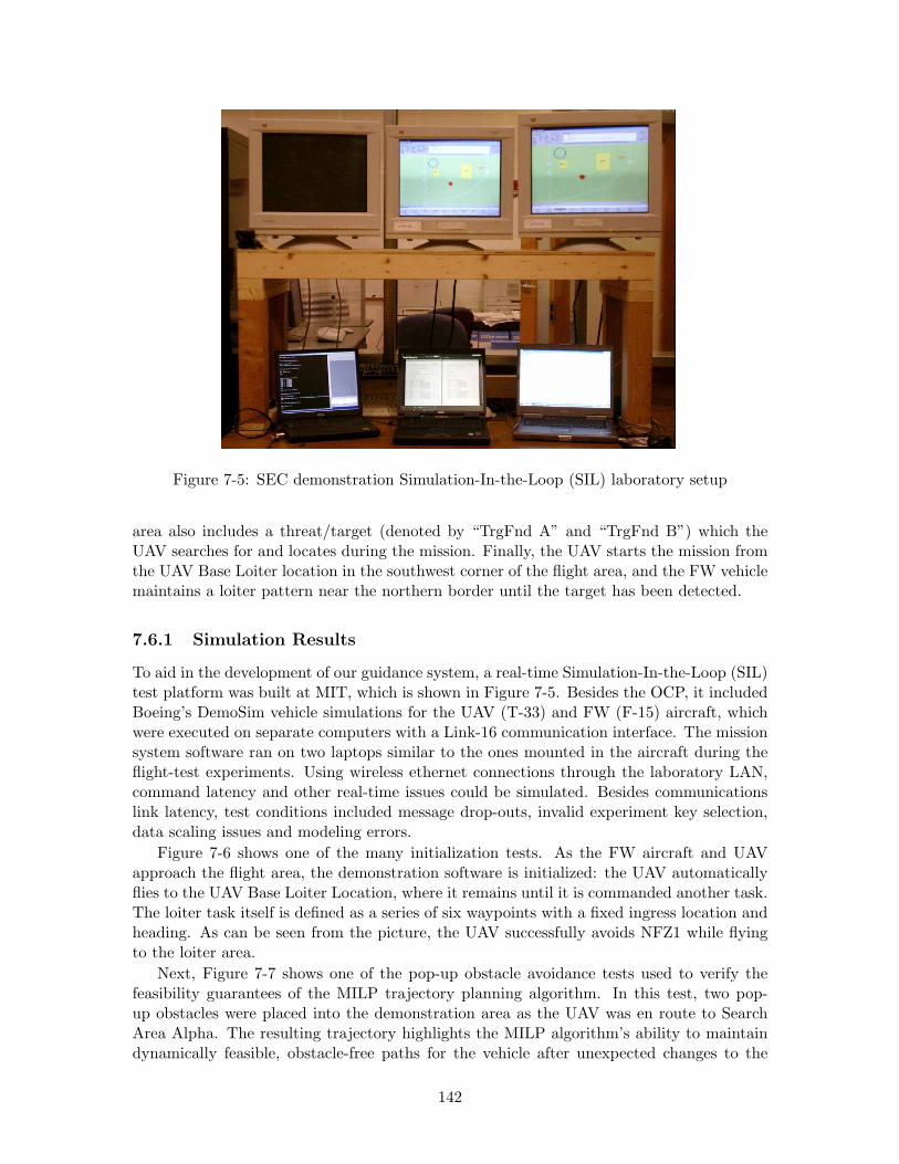
Figure 7-5: SEC demonstration Simulation-In-the-Loop (SIL) laboratory setup
area also includes a threat/target (denoted by “TrgFnd A” and “TrgFnd B”) which theUAV searches for and locates during the mission. Finally, the UAV starts the mission fromthe UAV Base Loiter location in the southwest corner of the flight area, and the FW vehiclemaintains a loiter pattern near the northern border until the target has been detected.
7.6.1 Simulation Results
To aid in the development of our guidance system, a real-time Simulation-In-the-Loop (SIL)test platform was built at MIT, which is shown in Figure 7-5. Besides the OCP, it includedBoeing’s DemoSim vehicle simulations for the UAV (T-33) and FW (F-15) aircraft, whichwere executed on separate computers with a Link-16 communication interface. The missionsystem software ran on two laptops similar to the ones mounted in the aircraft during theflight-test experiments. Using wireless ethernet connections through the laboratory LAN,command latency and other real-time issues could be simulated. Besides communicationslink latency, test conditions included message drop-outs, invalid experiment key selection,data scaling issues and modeling errors.
Figure 7-6 shows one of the many initialization tests. As the FW aircraft and UAVapproach the flight area, the demonstration software is initialized: the UAV automaticallyflies to the UAV Base Loiter Location, where it remains until it is commanded another task.The loiter task itself is defined as a series of six waypoints with a fixed ingress location andheading. As can be seen from the picture, the UAV successfully avoids NFZ1 while flyingto the loiter area.
Next, Figure 7-7 shows one of the pop-up obstacle avoidance tests used to verify thefeasibility guarantees of the MILP trajectory planning algorithm. In this test, two pop-up obstacles were placed into the demonstration area as the UAV was en route to SearchArea Alpha. The resulting trajectory highlights the MILP algorithm’s ability to maintaindynamically feasible, obstacle-free paths for the vehicle after unexpected changes to the
142
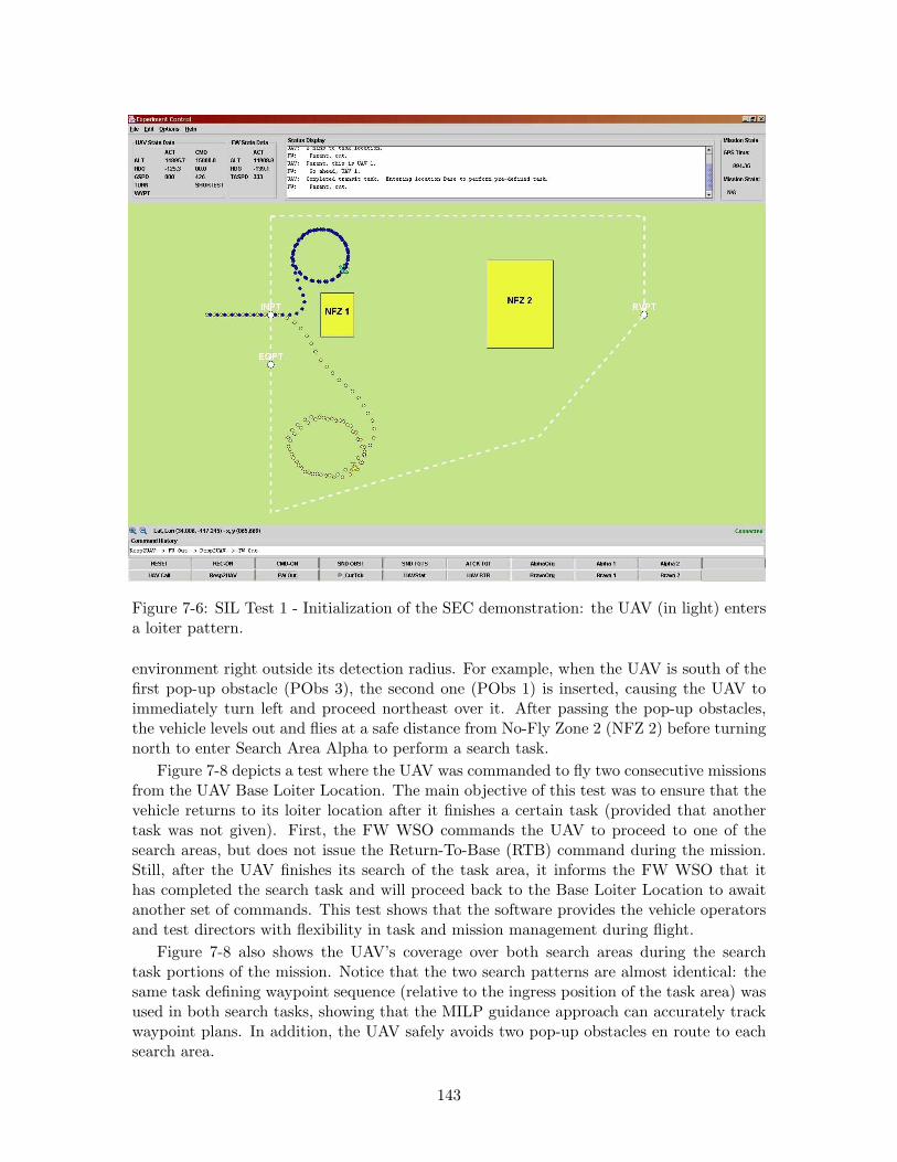
Figure 7-6: SIL Test 1 - Initialization of the SEC demonstration: the UAV (in light) entersa loiter pattern.
environment right outside its detection radius. For example, when the UAV is south of thefirst pop-up obstacle (PObs 3), the second one (PObs 1) is inserted, causing the UAV toimmediately turn left and proceed northeast over it. After passing the pop-up obstacles,the vehicle levels out and flies at a safe distance from No-Fly Zone 2 (NFZ 2) before turningnorth to enter Search Area Alpha to perform a search task.
Figure 7-8 depicts a test where the UAV was commanded to fly two consecutive missionsfrom the UAV Base Loiter Location. The main objective of this test was to ensure that thevehicle returns to its loiter location after it finishes a certain task (provided that anothertask was not given). First, the FW WSO commands the UAV to proceed to one of thesearch areas, but does not issue the Return-To-Base (RTB) command during the mission.Still, after the UAV finishes its search of the task area, it informs the FW WSO that ithas completed the search task and will proceed back to the Base Loiter Location to awaitanother set of commands. This test shows that the software provides the vehicle operatorsand test directors with flexibility in task and mission management during flight.
Figure 7-8 also shows the UAV’s coverage over both search areas during the searchtask portions of the mission. Notice that the two search patterns are almost identical: thesame task defining waypoint sequence (relative to the ingress position of the task area) wasused in both search tasks, showing that the MILP guidance approach can accurately trackwaypoint plans. In addition, the UAV safely avoids two pop-up obstacles en route to eachsearch area.
143
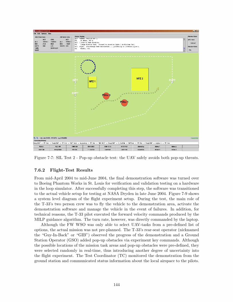
Figure 7-7: SIL Test 2 - Pop-up obstacle test: the UAV safely avoids both pop-up threats.
7.6.2 Flight-Test Results
From mid-April 2004 to mid-June 2004, the final demonstration software was turned overto Boeing Phantom Works in St. Louis for verification and validation testing on a hardwarein the loop simulator. After successfully completing this step, the software was transitionedto the actual vehicle setup for testing at NASA Dryden in late June 2004. Figure 7-9 showsa system level diagram of the flight experiment setup. During the test, the main role ofthe T-33’s two person crew was to fly the vehicle to the demonstration area, activate thedemonstration software and manage the vehicle in the event of failures. In addition, fortechnical reasons, the T-33 pilot executed the forward velocity commands produced by theMILP guidance algorithm. The turn rate, however, was directly commanded by the laptop.
Although the FW WSO was only able to select UAV-tasks from a pre-defined list ofoptions, the actual mission was not pre-planned. The T-33’s rear-seat operator (nicknamedthe “Guy-In-Back” or “GIB”) observed the progress of the demonstration and a GroundStation Operator (GSO) added pop-up obstacles via experiment key commands. Althoughthe possible locations of the mission task areas and pop-up obstacles were pre-defined, theywere selected randomly in real-time, thus introducing another degree of uncertainty intothe flight experiment. The Test Coordinator (TC) monitored the demonstration from theground station and communicated status information about the local airspace to the pilots.
144
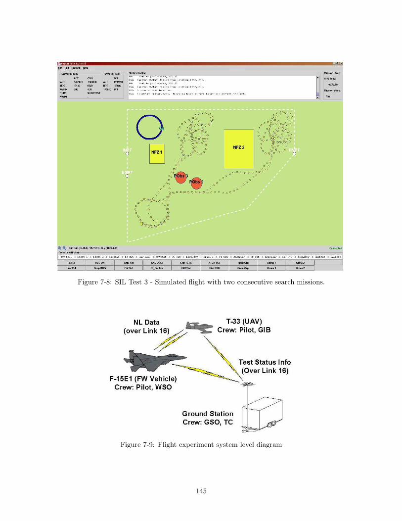
Figure 7-8: SIL Test 3 - Simulated flight with two consecutive search missions.
Figure 7-9: Flight experiment system level diagram
145
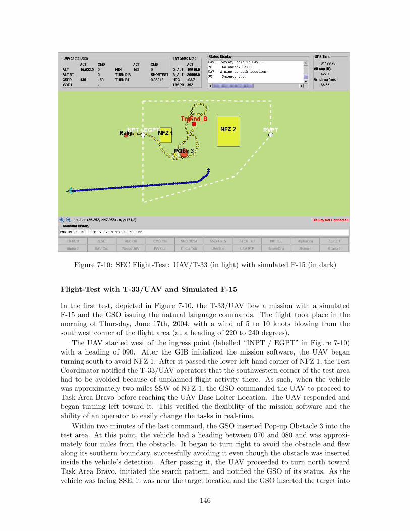
Figure 7-10: SEC Flight-Test: UAV/T-33 (in light) with simulated F-15 (in dark)
Flight-Test with T-33/UAV and Simulated F-15
In the first test, depicted in Figure 7-10, the T-33/UAV flew a mission with a simulatedF-15 and the GSO issuing the natural language commands. The flight took place in themorning of Thursday, June 17th, 2004, with a wind of 5 to 10 knots blowing from thesouthwest corner of the flight area (at a heading of 220 to 240 degrees).
The UAV started west of the ingress point (labelled “INPT / EGPT” in Figure 7-10)with a heading of 090. After the GIB initialized the mission software, the UAV beganturning south to avoid NFZ 1. After it passed the lower left hand corner of NFZ 1, the TestCoordinator notified the T-33/UAV operators that the southwestern corner of the test areahad to be avoided because of unplanned flight activity there. As such, when the vehiclewas approximately two miles SSW of NFZ 1, the GSO commanded the UAV to proceed toTask Area Bravo before reaching the UAV Base Loiter Location. The UAV responded andbegan turning left toward it. This verified the flexibility of the mission software and theability of an operator to easily change the tasks in real-time.
Within two minutes of the last command, the GSO inserted Pop-up Obstacle 3 into thetest area. At this point, the vehicle had a heading between 070 and 080 and was approxi-mately four miles from the obstacle. It began to turn right to avoid the obstacle and flewalong its southern boundary, successfully avoiding it even though the obstacle was insertedinside the vehicle’s detection. After passing it, the UAV proceeded to turn north towardTask Area Bravo, initiated the search pattern, and notified the GSO of its status. As thevehicle was facing SSE, it was near the target location and the GSO inserted the target into
146
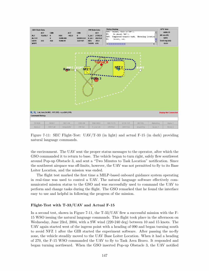
Figure 7-11: SEC Flight-Test: UAV/T-33 (in light) and actual F-15 (in dark) providingnatural language commands.
the environment. The UAV sent the proper status messages to the operator, after which theGSO commanded it to return to base. The vehicle began to turn right, safely flew southwestaround Pop-up Obstacle 3, and sent a “Two Minutes to Task Location” notification. Sincethe southwest airspace was off-limits, however, the UAV was not permitted to fly to its BaseLoiter Location, and the mission was ended.
The flight test marked the first time a MILP-based onboard guidance system operatingin real-time was used to control a UAV. The natural language software effectively com-municated mission status to the GSO and was successfully used to command the UAV toperform and change tasks during the flight. The GSO remarked that he found the interfaceeasy to use and helpful in following the progress of the mission.
Flight-Test with T-33/UAV and Actual F-15
In a second test, shown in Figure 7-11, the T-33/UAV flew a successful mission with the F-15 WSO issuing the natural language commands. This flight took place in the afternoon onWednesday, June 23rd, 2004, with a SW wind (220-240 deg) between 10 and 15 knots. TheUAV again started west of the ingress point with a heading of 090 and began turning southto avoid NFZ 1 after the GIB started the experiment software. After passing the no-flyzone, the vehicle steadily moved to the UAV Base Loiter Location. When it had a headingof 270, the F-15 WSO commanded the UAV to fly to Task Area Bravo. It responded andbegan turning northward. When the GSO inserted Pop-up Obstacle 3, the UAV notified
147
the F-15 that it detected the threat and successfully avoided the obstacle. As it approachedthe task area, the UAV informed the F-15 WSO that it was two minutes from the ingresspoint it was initially given. At that time, the WSO commanded the UAV to change theentrance location. It responded and proceeded to the new ingress point. This again verifiedthe flexibility of the task scheduling and trajectory planning software.
After reaching the task area, the UAV notified the F-15 WSO and began its searchpattern. As it turned left toward the southern boundary of the search area, the GSOinserted Target B into the environment. The UAV notified the F-15 WSO and sent animage. The F-15 WSO then commanded the UAV to return to base. The UAV acknowledgedthe command and flew back to its loiter location, avoiding obstacles and providing statusnotifications to the F-15 WSO along the way. The demonstration was ended when the UAVsuccessfully returned to the UAV Base Loiter Location.
This flight-test marked the first time that a natural language interface was used by amanned vehicle to task and command a UAV in real-time. The F-15 WSO also remarkedthat he found the interface easy to use and helpful in following the progress of the mission.In addition, the test marked the first time that an onboard MILP-based guidance system wasused to control a UAV in coordination with a manned vehicle. Furthermore, it was the firstsuccessful in-flight cooperation demonstration between the F-15 and UAV for the Boeingteam. Overall, both flight-tests provided an important proof-of-concept of the capabilitiesof the MIT mission software as previously witnessed in the laboratory: the flexibility of thetask scheduling software allowed the test team to make adjustments in real-time, while thetrajectory generation algorithm safely guided the UAV through the environment.
7.7 Conclusion
This chapter described the development, architecture and testing of a manned vehicle - UAVmission system that allows an operator in a manned aircraft to issue mission level commandsto an autonomous aircraft in real-time. A natural language interface was presented thatallows the manned and unmanned vehicle to communicate in languages understood by bothagents. A task scheduler transformed these commands into a dynamic mission plan con-sisting of task waypoints. The latter were then given to a real-time MILP-based trajectoryplanner, generating obstacle-free trajectories through a partially-known environment byimplementing the feasible receding horizon strategy presented in Chapter 4.
The complete mission system was successfully tested using high-fidelity software- andhardware in the loop simulations. Actual flight-test results with an F-15 and an autonomousT-33 were presented that provided an important proof-of-concept of the benefits and real-time capabilities of the natural language interface and MILP-based guidance methodology.After these first validation steps, the approach and algorithms are ready to being transi-tioned to larger problems, such as platforms with multiple unmanned vehicles running dis-tributed task assignment and trajectory planning strategies. The eventual goal is to havea single operator issue team level mission commands using natural language. We believethat in the future natural language interfaces will be the most efficient way to communicatewith unmanned vehicle systems.
148
Chapter 8
Conclusion
8.1 Summary
This thesis presented several new concepts and algorithms for online receding horizon tra-jectory planning of autonomous vehicles. We started off with a general problem formulationand used mixed-integer linear programming as the modeling and implementation framework.A new, more efficient approach to capture avoidance constraints for arbitrarily shaped ob-stacles was introduced. Next, the basic linear dynamics used in Chapter 2 were extended inChapter 3 to incorporate agile nonlinear behavior into the planning formulation. A hybridcontrol architecture for trajectory planning of agile vehicles was presented that combinesmultiple velocity control modes with a maneuver scheduler. The former provide the flexi-bility to precisely navigate between waypoints in a cluttered environment, while the latterenables execution of pre-programmed maneuvers at the limit of the vehicle capabilities.The closed-loop dynamics under this control architecture were described by a simple hybridmodel consisting of a set of LTI modes and discrete, fixed-duration state transitions. Onlinetrajectory optimization through cluttered environments was again formulated using MILP.The approach was worked out in detail for a small-scale helicopter model based on MIT’saerobatic X-Cell.
Chapter 4 then introduced the concept of a feasible invariant set that is a periodic,dynamically feasible and obstacle-free sequence of states in which a vehicle can remain foran indefinite period of time. Constraining all intermediate receding horizon trajectories toterminate in such sets guarantee feasibility of the planning problem at all future iterations.These terminal feasible invariant sets were expressed as a collection of affine transformationsof the last state in the planning horizon and as a result were computed online as part of theoptimization problem. An explicit formulation for a UAV was worked out using obstacle-free loitering circles as feasible invariant sets. Next, safety was defined as being able to leavethe terminal feasible invariant set at some time step in the future and backtrack along theexecuted trajectory. A receding horizon formulation that maintains safety and feasibility atall time steps was presented. A practical approach that only maintains safety was discussedas well.
In Chapter 5, the terminal feasible invariant set principle was used to design a distributedalgorithm for multi-vehicle path planning with feasibility guarantees. A receding horizonplanning strategy was adopted for each vehicle individually that accounts for the trajectoriesof the neighboring ones. Within one iteration of the algorithm, the vehicles update theirtrajectories in a sequential fashion. Feasibility at all times is guaranteed by constraining
149
the intermediate plans of all vehicles to terminate in individual feasible invariant sets. AMILP-based formulation for multiple aircraft using loiter circles was worked out in detail.
Chapter 6 presented a proof-of-concept application of online MILP-based trajectoryplanning for multiple vehicles. The problem of interest was to maintain line of sight com-munication in a cluttered environment between a mission vehicle and ground station usinga relay network. Both a centralized and a distributed formulation were given. The formerwas successfully implemented on two X-Cell helicopters and tested in a real-world scenario.
Chapter 7 then presented UAV flight-test results of the feasible receding horizon planningstrategy of Chapter 4. It discussed the development, architecture and testing of a mannedvehicle - UAV mission system that allows an operator in a manned aircraft to issue missionlevel commands to an autonomous aircraft in real-time. The complete mission system wassuccessfully tested using a manned F-15 and an autonomous T-33 aircraft. The results inboth chapters showed that receding horizon MILP-based trajectory planning is a flexibleframework and a feasible option for real-time guidance.
8.2 Future Work
The concepts introduced in this thesis give rise to various topics for future research. First,throughout the thesis, we only considered the nominal planning problem which does notaccount for external disturbances acting on the vehicle or uncertainties in the dynamicmodels. Introducing robustness in the planning problem is therefore a necessary next step.Among other, interesting problems related to robustness include handling uncertainties inthe location of obstacles and perturbations during maneuver execution of the LTI-MA,formulating robustly feasible invariant sets leading to robust feasibility and safety, andtackling uncertainties in the execution of the individual plans in the distributed planningalgorithm of Chapter 5. Some initial work on the last two issues was recently begun in [71]and [70].
A second broad topic is related to the performance and stability of the various planningformulations. For example, good cost-to-go functions for the LTI-MA that account forthe availability of maneuvers need to be developed. This may include functions that arecomputed offline and then incorporated in the online trajectory optimization. Functionsfor often recurring situations, such as turning around a corner or reversing direction, orfunctions corresponding to different planning modes as discussed in Chapter 3 could bedesigned. Good cost-to-go functions are required to prevent the vehicle from getting trappedin local minima. For the distributed multi-vehicle case, a related performance and stabilityconcern is the possible existence of live-lock situations, i.e. the condition when all vehiclesare trapped in their respective terminal feasible invariant sets. Proving that a particularobjective function or algorithm will be able to avoid such situations is another problem thathas to be tackled. Furthermore, comparing the performance of the distributed approachto centralized formulations with respect to the quality of the resulting trajectories and thetime required to compute them would be another interesting topic of future work.
Third, it may be worthwhile to investigate the specific structure of the MILP formu-lation for path planning in order to find specific heuristics and cuts in the MILP solutionalgorithms. Rather than fully relying on CPLEX to analyze the matrix structure and applyparticular heuristics or algorithms, guiding the optimization engine by exploiting a prioriknowledge of the problem structure could speed up the computation. Alternatively, com-bining the MILP approach with alternative approaches such as constraint programming
150

could take some of the computational load away as well.Finally, further implementation of the concepts developed in this thesis and testing of
various applications would be desirable. This includes actual helicopter flight-tests of theLTI-MA trajectory planning framework, possibly with the addition of flexible maneuversas introduced in [31], and demonstrations of the safe distributed algorithm for both ho-mogeneous and heteregenous vehicle teams. Work on the latter is currently already beingundertaken at MIT.
151

152
Bibliography
[1] M. Athans and P. Falb. Optimal Control, An Introduction to the Theory and ItsApplications. McGraw-Hill, 1966.
[2] J. Barraquand, L.E. Kavraki, J.C. Latombe, T.Y. Li, R. Motwani, and P. Raghavan.A random sampling scheme for path planning. International Journal of RoboticsResearch, 16(6):759–774, 1997.
[3] J. Barraquand, B. Langlois, and J.-C. Latombe. Numerical potential field techniquesfor robot path planning. IEEE Transactions on Systems, Man, and Cybernetics,22(2):224–241, March/April 1992.
[4] A. Bayen, E. Cruck, and C. Tomlin. Guaranteed overapproximations of unsafe sets forcontinuous and hybrid systems: Solving the Hamilton-Jacobi equation using viabilitytechniques. In C. Tomlin and M. Greenstreet, editors, Hybrid Systems: Computationand Control, volume 2289 of Lecture Notes in Computer Science (LNCS), pages 90–104. Springer Verlag, 2002.
[5] R. Beard and T. McLain. Multiple UAV cooperative search under collision avoidanceand limited range communication constraints. In Proc. 42nd IEEE Conference onDecision and Control, Maui, HI, December 2003.
[6] R. Beard, T. McLain, M. Goodrich, and E. Anderson. Coordinated target assign-ment and intercept for unmanned air vehicles. IEEE Transactions on Robotics andAutomation, 18(6):911–922, 2002.
[7] J. Bellingham, A. Richards, and J. How. Receding horizon control of autonomousaerial vehicles. In Proc. 2002 American Control Conference, pages 3741–3746, An-chorage, AK, May 2002.
[8] R. Bellman. Dynamic Programming. Princeton University Press, Princeton, NJ, 1957.
[9] A. Bemporad, F. Borrelli, and M. Morari. Piecewise linear optimal controllers forhybrid systems. In Proc. 2001 American Control Conference, volume 2, pages 1190–1194, Chicago, IL, June 2001.
[10] A. Bemporad, F. Borrelli, and M. Morari. Model predictive control based on lin-ear programming: the explicit solution. IEEE Transactions on Automatic Control,47(12):1974–1985, December 2002.
[11] A. Bemporad, A. De Luca, and G. Oriolo. Local incremental planning for a car-likerobot navigating among obstacles. In Proc. 1996 IEEE Int. Conference on Roboticsand Automation, pages 1205–1211, Minneapolis, MN, April 1996.
153
[12] A. Bemporad and M. Morari. Control of systems integrating logic, dynamics, andconstraints. Automatica, 35(3):407–427, 1999.
[13] A. Bemporad and M. Morari. Robust model predictive control: A survey. InA. Garulli, A. Tesi, and A. Vicino, editors, Robustness in Identification and Control,volume 245 of Lecture Notes in Control and Information Sciences, pages 207–226.Springer Verlag, 1999.
[14] A. Bemporad, M. Morari, V. Dua, and E.N. Pistikopoulos. The explicit solution ofmodel predictive control via multiparametric quadratic programming. In Proc. 2000American Control Conference, pages 872–876, Chicago, IL, June 2000.
[15] C. Bererton, G. Gordon, S. Thrun, and P. Khosla. Auction mechanism design formulti-robot coordination. In S. Thrun, L. Saul, and B. Scholkopf, editors, Proc. 2003Conference on Neural Information Processing Systems (NIPS). MIT Press, 2003.
[16] D.P. Bertsekas. Nonlinear Programming. Athena Scientific, Belmont, MA, 2nd edition,1999.
[17] D.P. Bertsekas. Dynamic Programming and Optimal Control, volume 1. AthenaScientific, Belmont, MA, 2nd edition, 2000.
[18] D. Bertsimas and J. N. Tsitsiklis. Introduction to Linear Optimization. AthenaScientific, Belmont, MA, 1997.
[19] D. Bertsimas and R. Weismantel. Optimization Over Integers. Dynamic Ideas, Bel-mont, MA, May 2005.
[20] J.T. Betts. Survey of numerical methods for trajectory optimization. AIAA Journalof Guidance, Control and Dynamics, 21(2):193–207, 1998.
[21] R. Bohlin and L.E. Kavraki. Path planning using lazy PRM. In Proc. 2000 IEEE Int.Conference on Robotics and Automation, pages 521–528, San Francisco, CA, April2000.
[22] F. Borrelli. Constrained Optimal Control of Linear and Hybrid Systems, volume 290of Lecture Notes in Control and Information Sciences. Springer-Verlag, Berlin Hei-delberg, May 2003.
[23] D. Brelaz. New methods to color the vertices of a graph. Comm. ACM, 22:251–256,1979.
[24] A.E. Bryson and Y.C. Ho. Applied Optimal Control: Optimization, Estimation, andControl. Hemisphere Publishing Corp., New York, 1975.
[25] S. Butenko, R. Murphey, and P. Pardalos (Eds.). Recent Developments in CooperativeControl and Optimization. Kluwer Academic Publishers, Norwell, MA, 2003.
[26] J. Canny. The Complexity of Robot Motion Planning. MIT Press, Cambridge, MA,1988.
[27] P.R. Chandler, M. Pachter, and S. Rasmussen. UAV cooperative control. In Proc.2001 American Control Conference, Arlington, VA, June 2001.
154
[28] P.R. Chandler, M. Pachter, D. Swaroop, J.M. Fowler, J.K. Howlett, S. Rasmussen,C.Schumacher, and K. Nygard. Complexity in UAV cooperative control. In Proc.2002 American Control Conference, Anchorage, AK, May 2002.
[29] H. Chen and F. Allgower. A quasi-infinite horizon nonlinear model predictive schemewith quaranteed stability. Automatica, 14(10):1205–1217, 1998.
[30] H. Choset. Sensor Based Motion Planning: the Hierarchical Generalized VoronoiGraph. PhD thesis, California Institute of Technology, Pasadena, CA, 1996.
[31] C. Dever, B. Mettler, E. Feron, and J. Popovic. Trajectory interpolation forparametrized maneuvering and flexible motion planning of autonomous vehicles. InProc. AIAA Guidance, Navigation, and Control Conference, number AIAA-2004-5143, Providence, RI, August 2004.
[32] W.B. Dunbar and R.M. Murray. Model predictive control of coordinated multi-vehicleformations. In Proc. 41st IEEE Conference on Decision and Control, pages 4631–4636,Las Vegas, NV, December 2002.
[33] C. A. Floudas. Nonlinear and Mixed-Integer Programming - Fundamentals and Ap-plications. Oxford University Press, Oxford, UK, 1995.
[34] R. Fourer, D. M. Gay, and B. W. Kernighar. AMPL, A modeling language for math-ematical programming. The Scientific Press, 1993.
[35] E Frazzoli. Robust Hybrid Control for Autonomous Vehicle Motion Planning. PhDthesis, Massachusetts Institute of Technology, Cambridge, MA, May 2001.
[36] E. Frazzoli, M. A. Dahleh, and E. Feron. Real-time motion planning for agile au-tonomous vehicles. AIAA Journal of Guidance, Control, and Dynamics, 25(1):116–129, 2002.
[37] E. Frazzoli, Z.-H. Mao, J.-H. Oh, and E. Feron. Resolution of conflicts involvingmany aircraft via semidefinite programming. AIAA Journal of Guidance, Controland Dynamics, 24(1):79–86, 2001.
[38] C.E. Garcia, D.M. Prett, and M. Morari. Model predictive control: Theory andpractice – a survey. Automatica, 25(3):335–348, 1989.
[39] V. Gavrilets. Autonomous Aerobatic Maneuvering of Miniature Helicopters. PhDthesis, Massachusetts Institute of Technology, Cambridge, MA, 2003.
[40] V. Gavrilets, E. Frazzoli, B. Mettler, M. Piedmonte, and E. Feron. Aggressive maneu-vering of small autonomous helicopters: A human-centered approach. InternationalJournal of Robotics Research, pages 795–807, October 2001.
[41] V. Gavrilets, I. Martinos, B. Mettler, and E. Feron. Aggressive maneuvering flighttests and simulation results of a miniature robotic helicopter. In Proc. 8th Interna-tional Symposium on Experimental Robotics, Sant’Angelo d’Ischia, Italy, July 2002.
[42] V. Gavrilets, I. Martinos, B. Mettler, and E. Feron. Flight test and simulation resultsfor an autonomous acrobatic helicopter. In Proc. 21st Digital Avionics Conference(DASC), Irvine, CA, October 2002.
155
[43] V. Gavrilets, B. Mettler, and E. Feron. Nonlinear model for a small-size acrobatichelicopter. In Proc. AIAA Guidance, Navigation, and Control Conference, Montreal,Canada, August 2001. AIAA Paper 2001-4333.
[44] V. Gavrilets, B. Mettler, and E. Feron. Human-inspired control logic for automatedmaneuvering of miniature helicopter. AIAA Journal of Guidance, Control and Dy-namics, 27(5), 2004.
[45] Google. Google earth. http://earth.google.com.
[46] J.R. Gossner, B. Kouvaritakis, and J.A. Rossiter. Stable generalized predictive controlwith constraints and bounded disturbances. Automatica, 33(4):551–568, 1996.
[47] D. Grundel, R. Murphey, and P. Pardalos (Eds.). Theory and Algorithms for Coop-erative Systems, volume 4 of Series on Computers and Operations Research. WorldScientific Publishing Co., Hackensack, NJ, 2004.
[48] J. Hauser and A. Jadbabaie. Aggressive maneuvering of a thrust vectored flying wing:a receding horizon approach. In Proc. 39th IEEE Conference on Decision and Control,pages 3582–3587, Sydney, Australia, December 2000.
[49] J.E. Hopcroft, J.T. Schwartz, and M. Sharir. On the complexity of motion planningfor multiple independent objects: PSPACE-hardness of the warehouseman’s problem.International Journal of Robotics Research, 4(3):76–88, 1984.
[50] A. Howard, M.J. Mataric, and G.S. Sukhatme. An incremental self-deployment al-gorithm for mobile sensor networks. Autonomous Robots, Special Issue on IntelligentEmbedded Systems, 13(2):113–126, 2002.
[51] D. Hsu, L.E. Kavraki, J-C. Latombe, R. Motwani, and S. Sorkin. On finding narrowpassages with probabilistic roadmap planners. In WAFR ’98: Proceedings of the ThirdWorkshop on the Algorithmic Foundations of Robotics on Robotics : the AlgorithmicPerspective, pages 141–153, March 1998.
[52] D. Hsu, J.-C. Latombe, and R. Motwani. Path planning in expansive configurationspaces. Int. Journal of Computational Geometry and Applications, 9(4):46–512, 1996.
[53] J. Hu, M. Prandini, and S. Sastry. Optimal coordinated maneuvers for three-dimensional aircraft conflict resolution. AIAA Journal of Guidance, Control andDynamics, 25(5):888–900, 2002.
[54] Y.K. Hwang and N. Ahuja. Gross motion planning - a survey. ACM Comp. Surv.,24(3):219–291, 1992.
[55] G. Inalhan, D. Stipanovic, and C. Tomlin. Decentralized optimization, with appli-cation to multiple aircraft coordination. In Proc. 41st IEEE Conference on Decisionand Control, Las Vegas, NV, December 2002.
[56] ILOG Inc. ILOG CPLEX 9.0 User’s guide. Mountain View, CA, 2003.
[57] A. Jadbabaie. Receding Horizon Control of Nonlinear Systems: A Control LyapunovFunction Approach. PhD thesis, California Institute of Technology, Pasadena, CA,October 2000.
156
[58] F. Jean. Complexity of nonholonomic motion planning. International Journal ofControl, 74(8):776–782, May 2001.
[59] N. Kalra, D. Ferguson, and A. Stentz. Hoplites: A market-based framework forplanned tight coordination in multirobot teams. In Proc. 2005 IEEE InternationalConference on Robotics and Automation, Barcelona, Spain, April 2005.
[60] T. Karatas and F. Bullo. Randomized searches and nonlinear programming in tra-jectory planning. In Proc.40th IEEE Conference on Decision and Control, December2001.
[61] L. Kavraki and J.-C. Latombe. Randomized preprocessing of configuration for fastpath planning. In Proc. 1994 IEEE International Conference on Robotics and Au-tomation, May 1994.
[62] L. Kavraki, P. Svestka, J. Latombe, and M. Overmars. Probabilistic roadmaps forpath planning in high-dimensional configuration spaces. Technical report, StanfordUniversity, Stanford, CA, 1994.
[63] L.E. Kavraki, F. Lamiraux, and C. Holleman. Probabilistic roadmaps for path plan-ning in high-dimensional configuration spaces. IEEE Transactions on Robotics andAutomation, 12(4):566–580, 1996.
[64] E.C. Kerrigan and J.M. Maciejowski. Invariant sets for constrained nonlinear discrete-time systems with application to feasibility in model predictive control. In Proc. 39thIEEE Conference on Decision and Control, Sydney, Australia, December 2000.
[65] O. Khatib. Real-time obstacle avoidance for manipulators and mobile robots. Inter-national Journal of Robotics Research, 1(5):90–98, 1986.
[66] M.V. Kothare, V. Balakrishnan, and M. Morari. Robust constrained model predictivecontrol using linear matrix inequalities. Automatica, 32(10):1361–1379, 1996.
[67] A. Kott. Advanced Technology Concepts for Command and Control. Xlibris Corpo-ration, Philadelphia, PA, 2004.
[68] Y. Kuwata and J. How. Stable trajectory design for highly constrained environmentsusing receding horizon control. In Proc. 2004 American Control Conference, pages902–907, Boston, MA, June 2004.
[69] Y. Kuwata and J. How. Three dimensional receding horizon control for UAVs. InProc. AIAA Guidance, Navigation, and Control Conference, Providence, RI, August2004. AIAA-2004-5144.
[70] Y. Kuwata, A. Richards, T. Schouwenaars, and J. How. Decentralized robust reced-ing horizon control for multi-vehicle guidance. Submitted to 2006 American ControlConference.
[71] Y. Kuwata, T. Schouwenaars, A. Richards, and J. How. Robust constrained recedinghorizon control for trajectory planning. In Proc. AIAA Guidance, Navigation, andControl Conference, San Francisco, CA, August 2005.
157
[72] J.-C. Latombe. Robot Motion Planning. Kluwer Academic Publishers, Norwell, MA,1991.
[73] J.-C. Latombe. Motion planning: a journey of robots, molecules, digital actors, andother artifacts. International Journal of Robotics Research, 18(11):1119–1128, Novem-ber 1999.
[74] S. M. LaValle. Planning Algorithms. Cambridge University Press, 2006. Also availableat http://msl.cs.uiuc.edu/planning/.
[75] S.M. LaValle and J.J. Kuffner. Randomized kinodynamic planning. In Proc. IEEEInternational Conference on Robotics and Automation, July 1999.
[76] T. Lemaire, R. Alami, and S. Lacroix. A distributed tasks allocation scheme inmulti-UAV context. In Proc. 2004 IEEE International Conference on Robotics andAutomation, pages 3622–3627, New Orleans, LA, April 2004.
[77] D. Leven and M. Sharir. An efficient and simple motion planning algorithm for aladder moving in two-dimensional space amidst polygonal barriers. Journal of Algo-rithms, 8:192–215, 1987.
[78] F-L. Lian and R. Murray. Cooperative task planning of multi-robot systems with tem-poral constraints. In Proc. 2003 IEEE Int. Conference on Robotics and Automation,Taipei, Taiwan, September 2003.
[79] F.-L. Lian and R.Murray. Real-time trajectory generation for the cooperative pathplanning of multi-vehicle systems. In Proc. 41st IEEE Conference on Decision andControl, pages 3766–3769, Las Vegas, NV, December 2002.
[80] T. Lozano-Perez. Spatial Planning with Polyhedral Models. PhD thesis, MassachusettsInstitute of Technology, June 1980.
[81] T. Lozano-Perez. Automaton planning of manipulator transfer movements. IEEETransactions on Systems, Man, and Cybernetics, 11(10):681–698, 1981.
[82] T. Lozano-Perez and M.A. Wesley. An algorithm for planning collision-free pathsamong polyhedral obstacles. Commun. ACM, 22(10):560–570, 1979.
[83] J. Lygeros, C. Tomlin, and S. Sastry. Controllers for reachability specifications forhybrid systems. Automatica, 35(3), March 1999.
[84] N. Lynch, R. Segala, and F. Vaandrager. Hybrid I/O automata revisited. In M.D. DiBenedetto and A. Sangiovanni-Vincentelli, editors, Hybrid Systems: Computation andControl, volume 2034 of Lecture Notes in Computer Science (LNCS), pages 403–417.Springer Verlag, 2001.
[85] J.M. Maciejowski. Predictive Control with Constraints. Prentice Hall, 2002.
[86] A. Makhorin. GLPK (GNU Linear Programming Kit). Available athttp://www.gnu.org/software/glpk/glpk.html.
[87] A. Marigo and A. Bicchi. Steering driftless nonholonomic systems by control quanta.In Proc. 37th IEEE Conference on Decision and Control, December 1998.
158
[88] K. Marti and S. Qu. Path planning for robots by stochastic optimization methods.International Journal of Intelligent and Robotic Systems, September 1997.
[89] I. Martinos, T. Schouwenaars, J. DeMot, and E. Feron. Hierarchical cooperative multi-agent navigation using mathematical programming. In Proc. 41th Annual AllertonConference on Communication, Control, and Computing, Monticello, IL, October2003.
[90] D.Q. Mayne. Control of constrained dynamic systems. European Journal of Control,7(2-3):87–99, 2001.
[91] D.Q. Mayne, J.B. Rawlings, C.V. Rao, and P.O.M. Scokaert. Constrained modelpredictive control: Stability and optimality. Automatica, 36(6):789–814, June 2000.
[92] C.R. McInnes. Potential function methods for autonomous spacecraft guidance andcontrol. In Proc. AAS/AIAA Astrodynamics Conference, pages 2093–2109, February1995.
[93] B. Mettler, M. Valenti, T. Schouwenaars, E. Frazzoli, and E. Feron. Rotorcraft mo-tion planning for agile maneuvering. In Proc. 58th Annual Forum of the AmericanHelicopter Society, Montreal, Canada, June 2002.
[94] B. Mettler, M. Valenti, T. Schouwenaars, Y. Kuwata, J. How, J. Paunicka, andE. Feron. Autonomous UAV guidance build-up: Flight-test demonstration and eval-uation plan. In Proc. AIAA Guidance, Navigation, and Control Conference, Austin,TX, August 2003. AIAA Paper 2003-5744.
[95] M.B. Milam, K. Mushambi, and R.M. Murray. A new computational approach to real-time trajectory generation for constrained mechanical systems. In Proc. 39th IEEEConference on Decision and Control, pages 845–851, Sydney, Australia, December2000.
[96] I. Mitchell, A. Bayen, and C. Tomlin. A time-dependent Hamilton-Jacobi formulationof reachable sets for continuous dynamic games. IEEE Transactions on AutomaticControl, 50(7):947–957, July 2005.
[97] I. Mitchell and C. Tomlin. Level set methods for computation in hybrid systems. InB. Krogh and N. Lynch, editors, Hybrid Systems: Computation and Control, volume1790 of Lecture Notes in Computer Science (LNCS), pages 310–323. Springer Verlag,2000.
[98] M. Morari and J. Lee. Model predictive control: Past, present and future. Computersand Chemical Engineering, 23(4):667–682, May 1999.
[99] J. De Mot and E. Feron. Spatial distribution of two-agent clusters for efficient naviga-tion. In Proc. 42nd IEEE Conference on Decision and Control, Maui, HI, December2003.
[100] H.G. Nguyen, N. Pezeshkian, M. Raymond, A. Gupta, and J.M. Spector. Autonomouscommunication relays for tactical robots. In Proc. 11th Int. Conference on AdvancedRobotics, Coimbra, Portugal, June 2003.
159
[101] Office of the Under Secretary of Defense for Acquisition, Technology and Logistics.Unmanned aerial vehicles roadmap 2002-2027, December 2002. Report Number:A809414.
[102] M. Oishi, C. Tomlin, V. Gopal, and D. Godbole. Addressing multiobjective control:Safety and performance through constrained optimization. In M.D. Di Benedettoand A. Sangiovanni-Vincentelli, editors, Hybrid Systems: Computation and Control,volume 2034 of Lecture Notes in Computer Science (LNCS), pages 459–472. SpringerVerlag, 2001.
[103] L. Pallottino, E. Feron, and A. Bicchi. Conflict resolution problems for air trafficmanagement systems solved with mixed integer programming. IEEE Transactions onIntelligent Transportation Systems, 3(1):3–11, 2002.
[104] G.J. Pappas, G. Lafferriere, and S. Sastry. Hierarchically consistent control systems.IEEE Transactions on Automatic Control, 45(6):1144–1160, June 2000.
[105] G.J. Pappas and S. Simic. Consistent hierarchies of nonlinear abstractions. In Proc.39th IEEE Conference on Decision and Control, pages 4379–4384, December 2000.
[106] J. Paunicka, B. Mendel, and D. Corman. The OCP - an open middleware solution forembedded systems. In Proc. 2001 American Control Conference, pages 3445–3450,Arlington, VA, June 2001.
[107] M. Powers and T. Balch. Value-based communication preservation for mobile robots.In Proc. 7th International Symposium on Distributed Autonomous Robotic Systems,Toulouse, France, June 2004.
[108] A. Raghunathan, V. Gopal, D. Subramanian, L. Biegler, and T. Samad. Dynamicoptimization strategies for three-dimensional conflict resolution of multiple aircraft.AIAA Journal of Guidance, Control and Dynamics, 27(4):586–594, 2004.
[109] J.B. Rawlings. Tutorial overview of model predictive control. IEEE Control SystemsMagazine, 20(3):38–52, June 2000.
[110] J. Reif. Complexity of the mover’s problem and generalizations. In Proc. 20th IEEESymposium on Foundations of Computer Science, pages 224–241, 1979.
[111] J.H. Reif and M. Sharir. Motion planning in the presence of moving obstacles. InProc. 25th IEEE Symposium on Foundations of Computer Science, pages 144–154,December 1985.
[112] A. Richards. Robust Constrained Model Predictive Control. PhD thesis, MassachusettsInstitute of Technology, Cambridge, MA, December 2004.
[113] A. Richards, J. Bellingham, M. Tillerson, and J. How. Coordination and controlof multiple UAVs. In Proc. AIAA Guidance, Navigation, and Control Conference,Monterey, CA, August 2002.
[114] A. Richards and J. How. Aircraft trajectory planning with collision avoidance usingmixed integer linear programming. In Proc. 2002 American Control Conference, pages1936–1941, Anchorage, AK, May 2002.
160
[115] A. Richards and J. How. Model predictive control of vehicle maneuvers with guaran-teed completion time and robust feasibility. In Proc. 2003 American Control Confer-ence, Denver, CO, June 2003.
[116] A. Richards, Y. Kuwata, and J. How. Experimental demonstrations of real-time MILPcontrol. In Proc. AIAA Guidance, Navigation, and Control Conference, Austin, TX,August 2003.
[117] A. Richards, T. Schouwenaars, J. How, and E. Feron. Spacecraft trajectory planningwith avoidance constraints using mixed-integer linear programming. AIAA Journalof Guidance, Control and Dynamics, 25(4):755–764, 2002.
[118] E. Roche. Parsing with finite-state transducers. In E. Roche and Y. Schabes, editors,Finite-State Language Processing. MIT Press, Cambridge, MA, 1997.
[119] A.B. Roger and C.R. McInnes. Safety constrained free-flyer path planning at theinternational space station. AIAA Journal of Guidance, Control, and Dynamics,23(6):971–979, 2000.
[120] J.A. Rossiter, B. Kouvaritakis, and J.R. Gossner. Guaranteeing feasibility in con-strained stable generalized predictive control. IEE Proc.-Control Theory Applications,143:463–469, 2001.
[121] E. Royer and C-K. Toh. A review of current routing protocols for ad hoc mobilewireless networks. IEEE Personal Communications, 6(2):46–55, 1999.
[122] T. Samad and G. Balas. Software-Enabled Control: Information Technology for Dy-namical Systems. Wiley-IEEE Press, Hoboken, NJ, 2003.
[123] D.P. Scharf, F.Y. Hadaegh, and S.R. Ploen. A survey of spacecraft formation flyingguidance and control (Part I): Guidance. In Proc. 2003 American Control Conference,pages 1733– 1739, June 2003.
[124] D.P. Scharf, F.Y. Hadaegh, and S.R. Ploen. A survey of spacecraft formation flyingguidance and control (Part II): Control. In Proc. 2004 American Control Conference,pages 2976– 2985, June 2004.
[125] T. Schouwenaars. Mixed integer programming for optimal collision-free path planningof autonomous vehicles. Master’s thesis, Katholieke Universiteit Leuven, Departmentof Electrical Engineering, Leuven, Belgium, May 2001.
[126] T. Schouwenaars, E. Feron, and J. How. Hybrid model for receding horizon guidanceof agile autonomous rotorcraft. In Proc. 16th IFAC Symposium on Automatic Controlin Aerospace, St. Petersburg, Russia, June 2004.
[127] T. Schouwenaars, B. De Moor, E. Feron, and J. How. Mixed integer programmingfor multi-vehicle path planning. In Proc. 2001 European Control Conference, pages2603–2608, Porto, Portugal, September 2001.
[128] T. Schouwenaars, B. Mettler, E. Feron, and J. How. Robust motion planning usinga maneuver automaton with built-in uncertainties. In Proc. 2003 American ControlConference, Denver, CO, June 2003.
161
[129] T. Schouwenaars, M. Valenti, E. Feron, and J. How. Implementation and flight testresults of MILP-based UAV guidance. In Proc. 2005 IEEE Aerospace Conference, BigSky, MT, March 2005.
[130] C. Schumacher, P.R. Chandler, and S. Rasmussen. Task allocation for wide areasearch munitions via network flow optimization. In Proc. 2002 American ControlConference, Anchorage, AK, May 2002.
[131] J.T. Schwartz and M. Sharir. On the piano movers’ problem: I. Communications onPure and Applied Mathematics, 36:345–398, 1983.
[132] J.T. Schwartz and M. Sharir. A survey of motion planning and related geometricalgorithms. Artificial Intelligence, 37(1-3):157–169, 1988.
[133] J.T. Schwartz and M. Sharir. Handbook of Theoretical Computer Science (vol. A):Algorithms and Complexity, chapter Algorithmic Motion Planning in Robotics, pages391–430. MIT Press, Cambridge, MA, 1990.
[134] P.O.M. Scokaert and D.Q. Mayne. Min-max feedback model predictive control forconstrained linear systems. IEEE Transactions on Automatic Control, 43(8):1136–1142, August 1998.
[135] P.O.M. Scokaert, D.Q. Mayne, and J.B. Rawlings. Suboptimal model predictivecontrol (feasibility implies stability). IEEE Transactions on Automatic Control,44(3):648–654, March 1999.
[136] P.O.M. Scokaert, J.B. Rawlings, and E.S. Meadows. Discrete-time stability withperturbations: Application to model predictive control. Automatica, 33(3):463–470,1997.
[137] D.H. Shim, H.J. Kim, and S. Sastry. Decentralized nonlinear model predictive controlof multiple flying robots in dynamic environments. In Proc. 43rd IEEE Conferenceon Decision and Control, Maui, HI, December 2003.
[138] K. Shin and N. McKay. A dynamic programming approach to trajectory planning ofrobotic manipulators. IEEE Transactions on Automatic Control, 31(6):491–500, June1986.
[139] L. Singh and J. Fuller. Trajectory generation for a UAV in urban terrain, using nonlin-ear MPC. In Proc. 2001 American Control Conference, pages 2301–2308, Arlington,VA, June 2001.
[140] J-J.E. Slotine and W. Li. Applied Nonlinear Control. Prentice Hall, Upper SaddleRiver, NJ, 1991.
[141] D. Spanos and R. Murray. Motion planning with wireless network constraints. InProc. 2005 American Control Conference, Portland, OR, June 2005.
[142] K. Sprague, V. Gavrilets, I. Martinos, D. Dugail, B. Mettler, and E. Feron. Designand applications of an avionics system for a miniature acrobatic helicopter. In Proc.20th Digital Avionics Systems (DASC), Daytona Beach, FL, October 2001.
162
[143] J. Sweeney, T.J. Brunette, Y. Yang, and R. Grupen. Coordinated teams of reactivemobile platforms. In Proc. 2002 IEEE Int. Conference on Robotics and Automation,Washington, D.C., May 2002.
[144] H.A. Taha. Operations Research, An Introduction. Macmillan Publishing Company,New York, 4th edition, 1987.
[145] C-K. Toh. Ad Hoc Mobile Wireless Networks: Protocols and Systems. Prentice HallPublishers, 2001.
[146] C. Tomlin, I. Mitchell, and R. Ghosh. Safety verification of conflict resolution ma-neuvers. IEEE Transactions on Intelligent Transportation Systems, 2(2), 2001.
[147] C. Tomlin, G.J. Pappas, and S. Sastry. Conflict resolution for air traffic management:a study in multi-agent hybrid systems. IEEE Transactions on Automatic Control,43(4):509–521, 1998.
[148] P. Ulam and R.C. Arkin. When good comms go bad: Communications recovery formulti-robot teams. In Proc. 2004 IEEE International Conference on Robotics andAutomation, pages 3727–3734, New Orleans, LA, April 2004.
[149] M. Valenti, T. Schouwenaars, Y. Kuwata, E. Feron, J. How, and J. Paunicka. Im-plementation of a manned vehicle-UAV mission system. In Proc. AIAA Guidance,Navigation, and Control Conference, Providence, RI, August 2004.
[150] A. Wagner and R. Arkin. Multi-robot communication-sensitive reconnaissance. InProc. 2004 IEEE International Conference on Robotics and Automation, pages 4674–4681, New Orleans, LA, April 2004.
[151] C.W. Warren. Multiple robot path coordination using artificial potential fields. InProc. 1990 IEEE Int. Conference on Robotics and Automation, pages 500–505, Cincin-nati, OH, May 1990.
[152] W.L. Winston. Operations Research, Algorithms and Applications. Duxbury Press,Belmont, CA, 3th edition, 1994.
[153] J. Wohletz, D. Castanon, and M. Curry. Closed-loop control for joint air operations.In Proc. 2001 American Control Conference, pages 4699–4704, Arlington, VA, June2001.
163


![Autonomous vehicles[1]](https://img.pdfslide.us/doc/110x75/54bf07bb4a7959cb478b4592/autonomous-vehicles1.jpg)