Embed Size (px)
Citation preview

Saad, Abdullah Aziz (2012) Cyclic plasticity and creep of power plant materials. PhD thesis, University of Nottingham.
Access from the University of Nottingham repository: http://eprints.nottingham.ac.uk/12538/1/PhD_thesis_-_Abdullah_Aziz_Saad.pdf
Copyright and reuse:
The Nottingham ePrints service makes this work by researchers of the University of Nottingham available open access under the following conditions.
This article is made available under the University of Nottingham End User licence and may be reused according to the conditions of the licence. For more details see: http://eprints.nottingham.ac.uk/end_user_agreement.pdf
For more information, please contact [email protected]
Cyclic Plasticity and Creep of
Power Plant Materials
Abdullah Aziz Saad, MSc
Thesis submitted to the University of Nottingham
for the degree of Doctor of Philosophy
MARCH 2012
i
Abstract
The thermo-mechanical fatigue (TMF) of power plant components is caused by the
cyclic operation of power plant due to startup and shutdown processes and due to
the fluctuation of demand in daily operation. Thus, a time-dependent plasticity
model is required in order to simulate the component response under cyclic thermo-
mechanical loading. The overall aim behind this study is to develop a material
constitutive model, which can predict the creep and cyclic loading behaviour at high
temperature environment, based on the cyclic loading test data of the P91 and the
P92 steels.
The tests on all specimens in the study were performed using the Instron 8862 TMF
machine system with a temperature uniformity of less than ±10°C within the gauge
section of the specimen. For the isothermal tests on the P91 steel, fully-reversed,
strain-controlled tests were conducted on a parent material of the steel at 400, 500
and 600˚C. For the P92 steel, the same loading parameters in the isothermal tests
were performed on a parent material and a weld metal of the steels at 500, 600 and
675°C. Strain-controlled thermo-mechanical fatigue tests were conducted on the
parent materials of the P91 and the P92 steels under temperature ranges of 400-
600°C and 500-675°C, respectively, with in-phase (IP) and out-of-phase (OP)
loading. In general, the steels exhibit cyclic softening behaviour throughout the
cyclic test duration under both isothermal and anisothermal conditions.
The cyclic softening behaviour of the P91 steel was further studied by analyzing
stress-strain data at 600°C and by performing microstructural investigations.
Scanning electron microscope (SEM) and transmission electron microscope (TEM)
images were used to investigate microstructural evolution and the crack initiation of
ii
the steel at different life fractions of the tests. The TEM images of the interrupted
test specimens revealed subgrain coarsening during the cyclic tests. On the other
hand, the SEM images showed the initiation of microcracks at the end of the
stabilisation period and the cracks were propagated in the third stage of cyclic
softening.
A unified, Chaboche, viscoplasticity model, which includes combined isotropic
softening and kinematic hardening with a viscoplastic flow rule for time-dependent
effects, was used to model the TMF behaviour of the steels The constants in the
viscoplasticity model were initially determined from the first cycle stress-strain data,
the maximum stress evolution during tests and the stress relaxation data. Then, the
initial constants were optimized using a least-squares optimization algorithm in
order to improve the general fit of the model to experimental data. The prediction of
the model was further improved by including the linear nonlinear isotropic hardening
in order to obtain better stress-strain behaviour in the stabilisation period.
The developed viscoplasticity model was subsequently used in the finite element
simulations using the ABAQUS software. The focus of the simulation is to validate
the performance of the model under various types of loading. Simulation results
have been compared with the isothermal test data with different strain ranges and
also the anisothermal cyclic testing data, for both in-phase and out-of-phase
loadings. The model’s performance under 3-dimensional stress conditions was
investigated by testing and simulating the P91 steel using a notched specimen
under stress-controlled conditions. The simulation results show a good comparison
to the experimental data.
iii
List of publications
1. Saad A. A., Hyde C. J., Sun W. and Hyde T. H. Thermal-mechanical fatigue
simulation of a P91 steel in a temperature range of 400-600˚C. Materials at
High Temperature 28 (3), 212-218, 2011.
2. Saad A. A., Sun W., Hyde T. H., and Tanner D. W. J. Cyclic softening
behaviour of a P91 steel under low cycle fatigue at high temperature.
Procedia Engineering 10, 1103-1108, 2011.
3. Saad A. A., Hyde T. H., Sun W. and Hyde C. J. Constitutive model
development of P91 steel and its simulation in TMF conditions. ESIA11
Conf. on Engineering Structural Integrity Assessment. 25-24 May 2011,
Manchester, UK.
4. Hyde C. J., Sun W., Hyde T. H., Saad A. A. Thermo-mechanical fatigue
testing and simulation using a viscoplasticty model. 21st Int. Workshop on
Computational Mechanics of Materials, 22-24 August 2011, Limerick,
Ireland.
5. Saad A. A., Hyde C. J., Sun W. and Hyde T. H. Thermal-mechanical fatigue
simulation of a P91 steel in a temperature range of 400-600°C. HIDA-5 Int.
Conf., 23-25 June 2010, Guildford, UK.
6. Hyde C. J., Sun W., Hyde T. H., Saad A. A. Thermo-mechanical fatigue
testing and simulation using a viscoplasticity model. (Accepted for Journal of
Computational Materials Science).

iv
Acknowledgements
I would like to take this opportunity to express my gratitude to my supervisors,
Professor Thomas Hyde and Dr Wei Sun, for their expertise, continued support and
valuable advice during my PhD study. Also, I would like to thank Professor Sean
Leen for his supervision during the first year of my research.
I wish to thank the technical staffs from the Department of Mechanical, Materials
and Manufacturing Engineering of the University of Nottingham, particularly Mr
Thomas Buss and Mr Brian Webster for their help with the experimental aspects of
this work. Thank you to Dr Nigel Neate, Mr Keith Dinsdale and Mr Martin Roe, for
the training in handling the SEM and TEM equipments. Also, I thank my fellow
researchers in the University Technology Centre and the Structural Integrity and
Dynamics group for their friendship and knowledge sharing.
I must thank Universiti Sains Malaysia and Ministry of Higher Education Malaysia for
financial support through academic staff training program, which enable me to
further my study in the University of Nottingham. Also, I would like to acknowledge
the support of EPSRC through the Supergen 2 programme and its industrial
partners for their valuable contributions to my project.
Finally, I would like to express my special thanks to my wife, Zuraihana Bachok, and
my kids for their love and support during my study in Nottingham. Also, I thank my
family members and friends for their support and encouragement.
v
Nomenclature
D Damage
EBSD Electron backscatter diffraction
FE Finite element
IP In-phase
LB Lower bound
N Number of cycles to reach the beginning of linear softening stage sta
N Number of cycles to reach the final softening stage tan
N Number of cycles to failure f
N Final number of cycles applied in the cyclic test fin
OP Out-of-phase
PID Proportional, integral and derivative
SEM Scanning electron microscopy
TC Thermocouple
TEM Transmission electron microscopy
TMF Thermo-mechanical fatigue
UB Upper bound
vi
List of contents Abstract i
List of publications iii
Acknowledgements iv
Nomenclature v
List of contents vi
Chapter 1 - Introduction 1
1.1 Background 1
1.2 Objectives 2
1.3 Thesis outline 3
Chapter 2 – Literature review 5
2.1 Overview 5
2.2 Introduction to material behaviour modelling 5
2.3 Elastic and plastic deformation 6
2.4 Cyclic plasticity 8
2.4.1 Isotropic hardening model 8
2.4.2 Kinematic hardening model 12
2.4.3 Combined isotropic-kinematic hardening model 17
2.5 Time-dependent cyclic plasticity 17
2.5.1 Uncoupled elastoplasticity-creep 17
2.5.2 Unified viscoplasticity model 18
2.5.3 Two-layer viscoplasticity model 22
2.6 Material behaviour under TMF conditions 24
2.7 P91 and P92 steel 27
2.7.1 Introduction to P91 and P92 steel 27
2.7.2 The microstructure 30
2.7.3 The microstructural evolution under cyclic loading test 32
Chapter 3 – Experimental work 38
3.1 Overview 38
3.2 Testing facilities 38
vii
3.3 Material and specimen preparation 40
3.4 Testing procedures for the P91 steel 42
3.4.1 Isothermal cyclic plasticity test of P91 steel 43
3.4.2 Thermomechanical fatigue testing of P91 steel 49
3.4.3 Cyclic notched bar test of P91 steel 51
3.5 Testing procedures for the P92 steel 53
3.6 Experimental results 57
3.6.1 Strain-controlled cyclic loading test 57
3.6.2 Hold period test 63
3.6.3 TMF test results 64
3.6.4 Notched specimen test results 67
Chapter 4 – Stress-strain analysis and microstructure investigation of
cyclic test 70
4.1 Overview 70
4.2 Stress-strain analysis 70
4.2.1 Determination of Nsta, Ntan and N 72 f
4.2.2 Young’s modulus analysis 73
4.2.3 Hysteresis loop area analysis 76
4.3 Fatigue model 82
4.3.1 Strain-based model 83
4.3.2 Energy-based model 84
4.4 Microstructure investigation 85
4.4.1 Scanning electron microscopy 86
4.4.2 Transmission electron microscopy 86
4.4.3 The microstructure investigation results 87
4.5 Discussions on the cyclic softening mechanisms 96
4.6 Conclusions 98
Chapter 5 – Viscoplasticity model development 100
5.1 Overview 100
5.2 The viscoplasticity model 100
5.3 The initial constants of the viscoplasticity model 103
5.3.1 Identification of initial yield stress and Young’s modulus 103
5.3.2 Identification of isotropic hardening parameters 104
5.3.3 Identification of kinematic hardening parameters 105
viii
5.3.4 Identification of Z and n constants 111
5.4 Constants optimisation 113
5.4.1 Two objective function optimisation 114
5.4.2 Three objective function optimisation 129
5.5 Two stages of isotropic hardening 136
5.6 Conclusions 141
Chapter 6 – Finite element simulation using the viscoplasticity model 142
6.1 Overview 142
6.2 Implementation of the viscoplasticity model in ABAQUS 142
6.3 FE simulation of the isothermal cyclic loading 144
6.4 FE simulation of the isothermal notched specimen 150
6.5 FE simulation of anisothermal fatigue loading 157
6.6 Conclusions 166
Chapter 7 – Conclusions and future work 167
7.1 Conclusions 167
7.2 Future work 169
References 171
Appendices 180
Chapter 1 ________ __________________________________________________ Introduction
1
Chapter 1 - Introduction
1.1 Background
The need for the power generation industry to improve the thermal efficiency of
power plant has led to the development of 9-12%Cr martensitic steels (Ennis et al.,
2003). The research on these materials has focussed on its creep strength, due to
its intended application at high temperature. However, understanding the thermo-
mechanical behaviour of power plant materials has become more important as the
current operation involves more cyclic operation, which has introduced the
possibility of thermo-mechanical fatigue (TMF) problems.
The required cyclic operation of power plant due to market forces and competition
has increased the concern of researchers on creep-fatigue interaction behaviour.
During start up, shut down or load changes of power plant operation, severe thermal
gradients between the inside and outside of components due to rapid rates of
change of steam temperatures may cause high stress levels to develop (Shibli and
Starr, 2007). For instance, bore cracking was found in power plant components and
it has been associated with thermal fatigue loading (Brett, 2003). To avoid thermal
fatigue, caused by frequent cycling, one solution is to utilise higher creep strength
alloy steels for pressure vessel construction (Shibli, 2008) so that the thickness of
the power plant components can be reduced. However, the stress-strain behaviour
of new power plant components needs to be understood first. This can be predicted
by finite element simulation as previously modelled by Hyde et al. (2003) for pipe
weldments under creep conditions at high temperature. The simulation of the
components requires a suitable constitutive material model which can accurately
predict the stress-strain behaviour and the failure life.
Chapter 1 ________ __________________________________________________ Introduction
2
The majority of previous studies on power plant materials have been related to the
creep behaviour under constant load operation. For example, creep constitutive
equations have been developed for the parent, heat-affected zone (HAZ) and weld
materials of Cr-Mo-V steel welds in the range 565-640˚C (Hayhurst et al., 2005).
Similar studies have been carried out, for a P91 steel, in order to develop a creep
constitutive model with a damage capability (Hyde et al, 2006). The development of
these creep constitutive models have contributed to the gaining of a better
understanding of the material behaviour in such applications as welding process
modelling (Yaghi et al., 2008) and failure prediction in multiaxial components
(Hayhurst et al., 2008).
In contrast to the above applications, the constitutive models which deal with creep
and cyclic loading conditions of power plant materials have had relatively little
attention. Thus, a model which can include both cyclic and viscous effects is
required. A commonly used model is the unified viscoplasticity model originally
developed by Chaboche (Chaboche and Rousselier, 1983). This viscoplasticity
model has been used in many researches, including the studies on aeroengine
materials such as nickel-base alloys (Yaguchi et al., 2002). However, the
viscoplasticity model is rarely used to represent the behaviour of power plant
materials.
1.2 Objectives
The objectives of the research are:
• To obtain quality stress-strain data from the P91 and the P92 steels under
cyclic plasticity and creep conditions in isothermal and anisothermal tests
using an available testing machine systems in the University of Nottingham;
Chapter 1 ________ __________________________________________________ Introduction
3
• To develop material constitutive models for P91 and P92 steels which can
accurately predict their creep and cyclic plasticity behaviour in a high
temperature environments;
• To investigate the cyclic softening behaviour of the steels by analyzing the
stress-strain behaviour and observing the microstructural evolutions
throughout the lifetime of the steels;
• To implement the viscoplasticity model in a commercial finite element
software and simulate the stress-strain behaviour of the steels under
thermo-mechanical fatigue loading conditions.
1.3 Thesis Outline
Chapter 2 presents the literature review on the material constitutive model which
includes typical cyclic plasticity components, such as kinematic and isotropic
hardening, and also a viscoplasticity model. Examples of previous work on material
behaviour modelling under cyclic thermo-mechanical conditions are also presented.
The developments of the P91 and the P92 steels used in the study are briefly
introduced.
The experimental equipment and procedures used for the isothermal and
anisothermal tests are described in Chapter 3. The details of the materials used, the
geometries of the specimens and the implemented loading in the testing
programmes are presented. Typical results of the tests are reported at the end of
this chapter.
In Chapter 4, the experimental stress-strain data, particularly for the P91 steel at
600°C, are further analyzed in order to understand the steel’s evolution under cyclic
loading. The results of microstructure investigation of the steel at different life
Chapter 1 ________ __________________________________________________ Introduction
4
fractions of the tests using scanning and transmission electron microscopes are
also presented.
Chapter 5 presents the development of the unified viscoplasticity model for the P91
and the P92 steels using the isothermal strain-controlled test data. The procedures
for determining the initial material constants are described. Then, the optimisation
programme, used to improve the stress-strain prediction of the model, is described
and the predicted results are compared to the experimental data. A modification to
the isotropic hardening model is also presented in order to improve the cyclic
softening prediction of the steels.
In Chapter 6, finite element simulations of the steels’ behaviour using the
viscoplasticity model using a commercial finite element software, ABAQUS, are
described. Simulation results of an axisymmetric model under isothermal conditions
at various strain ranges, a notched specimen model under isothermal stress-
controlled condition and an axisymmetric model under cyclic thermo-mechanical
conditions are compared to experimental data to validate the prediction capability of
the developed model.
Finally, Chapter 7 presents the overall research conclusions and suggests the
possible future work.
Chapter 2 ________ ______________________________________________ Literature review
5
Chapter 2 – Literature review
2.1 Overview
This literature review chapter is mainly concerned with material constitutive models
in relation to the steels used in this study, namely P91 and P92 steels. As the
material deforms cyclically under thermomechanical fatigue loading conditions,
plastic behaviour becomes important and the strain hardening behaviours such as
isotropic and kinematic hardening are reviewed in this Chapter. This chapter also
includes information on the development of the P91 and P92 steels, which have
been specifically developed for power plant applications and designed to have a
specific microstructure, in order to produce steels with good high temperature
mechanical behaviour.
2.2 Introduction to material behaviour modelling
In general, a material behaviour model is used to describe the stress-strain
behaviour of a material. It can be divided into two classes (Charkaluk et al., 2002).
The first model class is a physically-based model type representing a mechanical
behaviour by considering microstructure evolutions of materials. This kind of model
is used to represent both microscopic phenomena, such as microstructure
evolution, and macroscopic mechanical behaviour, such as creep and relaxation, on
a material scale. For example, cyclic softening behaviour of the martensitic 9Cr1Mo
steel has been modelled by analyzing and measuring the dislocation density using
transmission electron microscopy; the microstructure size and the macroscopic
stresses of cyclic softening phenomenon can then be predicted (Sauzay et al.,
2005, Sauzay et al., 2008). The second model class is a phenomenological-based
model type based on the results of mechanical tests on a material. This material
model is used to predict the stress-strain behaviour of a material and the model can
Chapter 2 ________ ______________________________________________ Literature review
6
be further used to predict the stress-strain behaviour of a mechanical structure
using, typically, a finite element simulation. The second model will be the focus of
this study.
2.3 Elastic and plastic deformation
When a load is applied to a body, a deformation will occur in either elastic or elastic-
plastic conditions, which depends on the magnitude of the applied load. In the
elastic deformation range, the body is returned to its original shape when the load is
removed. On the other hand, plastic deformation is irreversible and occurrs when
the load is such that some position within the component exceeds the elastic limit.
In terms of the physics of the phenomena, the elastic deformation involves a
variation in the interatomic distances without changes of place while plastic
deformation modifies interatomic bonds caused by slip movement in the
microstructure of the material (Lemaitre and Chaboche, 1994).
As reported by Timoshenko (1953), Robert Hooke studied the elasticity
phenomenon by measuring how far a wire string, of around 30 feet in length
deformed under an applied load. In the test, the magnitude of the extension was
found to be proportional to the applied weight. Thus, the deformation of an elastic
spring is generally described mathematically by the following equation:
kxF = (2.1)
where F is applied force, x is associated displacement and k is the proportionality
factor, which is often referred to as the spring constant.
Based on equation 2.1, the force and the displacement characteristics depend on
the size of the measured body. Thus, stress, σ , which refers to the ratio of the
applied force to the cross sectional area, and strain, ε , which refers to the ratio of
Chapter 2 ________ ______________________________________________ Literature review
7
the extension to the initial length, are introduced to eliminate the geometrical factors
(Callister, 2000). Equation 2.1 can be rewritten as:
εσ E= (2.2)
where E is proportionality constant which is often referred to as the Young’s
modulus or the modulus of elasticity (Hertzberg, 1996) for the material. Equation 2.2
is also known as Hooke’s law, which describes the linear stress-strain response of a
material.
Plastic deformation occurs when the applied load (or stress) exceeds a certain level
of stress called the elastic limit. Above this limit, the stress is no longer proportional
to strain. However, the exact stress at which this limit occurs is difficult to determine
experimentally as it depends on the accuracy of the strain measurement device
used. Thus, a conventional elastic limit or a yield stress value is determined by
constructing a straight line parallel to the linear elastic stress-strain curve at a
specified strain offset, commonly 0.2%. The intersection point between the parallel
line and the experimental curve is taken as the yield stress (0.2% proof stress)
value. For example, the yield stress value of P91 steel at room temperature with a
0.2% criterion is 415 MPa (Vaillant et al., 2008). In some cases, a lower strain offset
of 0.02% is used when the permanent strain obtained with the former criterion is
high when compared to the elastic strain (Lemaitre and Chaboche, 1994).
Irreversible deformation may also happen at stresses below the conventional elastic
limit if the load is maintained for a long time. This type of deformation is referred to
as creep, the magnitude of which is a function of stress, time and temperature. The
creep effect is significant at high temperatures and is generally significant when the
temperature of the material is greater than approximately 0.4 of the absolute melting
temperature, Tm. A creep test is conducted by applying a constant load to a
Chapter 2 ________ ______________________________________________ Literature review
8
specimen, which results in three stages of creep deformation. In the primary stage,
the strain rate decreases with time as the material approaches a steady-state stage.
The creep strain increases steadily in the secondary stage with a constant,
minimum, strain rate. Finally, the strain rate accelerates during tertiary creep until
final failure occurs (Bhadeshia, 2003; Evans and Wilshire, 1985). The secondary
stage of creep usually occupies the longest period of time in a creep test and the
steady-state creep rate behaviour is usually expressed by a power law, also
referred to as Norton’s law, which is given by the following equation:
nAσε = (2.3)
where A and n are material constants which can be determined from data
obtained in the secondary stage.
2.4 Cyclic plasticity
When subjected to cyclic loading condition, the plastic deformations which occur in
materials exhibit several phenomena such as the Bauschinger effect, cyclic
hardening/softening and material ratchetting. The cyclic loading of a material, under
tension-compression conditions, produces a hysteresis loop. The stress-strain
behaviour which occurs under cyclic loading, with time independent effects are
normally represented by isotropic hardening, kinematic hardening or some
combination of both the isotropic and kinematic hardening models.
2.4.1 Isotropic hardening model
Isotropic hardening describes the change which occurs in the equivalent stress,
defining the size of the yield surface, as a function of accumulated plastic strain. A
schematic description of the isotropic hardening model is shown in Figure 2.1.
Chapter 2 ________ ______________________________________________ Literature review
9
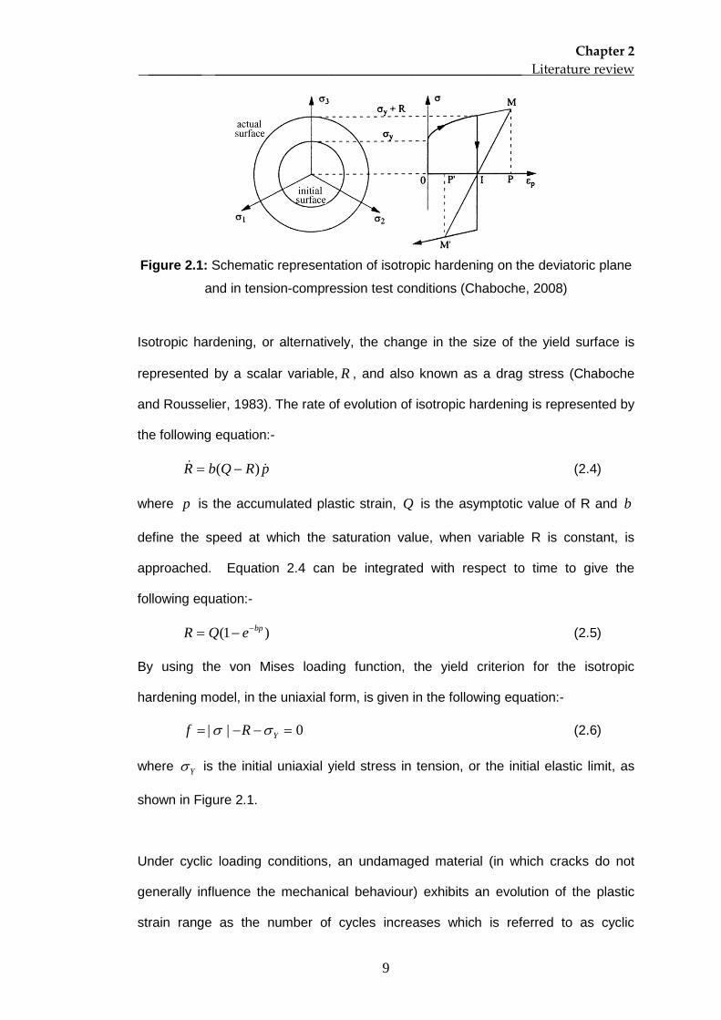
Figure 2.1: Schematic representation of isotropic hardening on the deviatoric plane
and in tension-compression test conditions (Chaboche, 2008)
Isotropic hardening, or alternatively, the change in the size of the yield surface is
represented by a scalar variable, R , and also known as a drag stress (Chaboche
and Rousselier, 1983). The rate of evolution of isotropic hardening is represented by
the following equation:-
pRQbR )( −= (2.4)
where p is the accumulated plastic strain, Q is the asymptotic value of R and b
define the speed at which the saturation value, when variable R is constant, is
approached. Equation 2.4 can be integrated with respect to time to give the
following equation:-
)1( bpeQR −−= (2.5)
By using the von Mises loading function, the yield criterion for the isotropic
hardening model, in the uniaxial form, is given in the following equation:-
0|| =−−= YRf σσ (2.6)
where Yσ is the initial uniaxial yield stress in tension, or the initial elastic limit, as
shown in Figure 2.1.
Under cyclic loading conditions, an undamaged material (in which cracks do not
generally influence the mechanical behaviour) exhibits an evolution of the plastic
strain range as the number of cycles increases which is referred to as cyclic
Chapter 2 ________ ______________________________________________ Literature review
10
hardening or cyclic softening behaviour. The cyclic hardening of a material refers to
the decrease of the plastic strain range, associated with an increase of the stress
amplitude with increasing number of cycles in a cyclic test. This is observed under
strain-controlled test conditions. This behaviour has been observed in many
materials such as 316 stainless steel (Hyde et al., 2010; Kim et al., 2008; Mannan
and Valsan, 2006), high nickel-chromium materials (Leen et al., 2010) and nickel-
based superalloys (Zhan et al, 2008; Kim et al., 2007; Yaguchi et al., 2002). On the
other hand, the plastic strain range increases as cyclic loading continues in a
material, exhibiting cyclic softening behaviour such as is found to occur in a
55NiCrMoV8 (Bernhart et al., 1999) and 9Cr-1Mo steel (Nagesha et al., 2002;
Shankar et al., 2006; Fournier et al., 2006; Fournier et al., 2009a). The cyclic
hardening phenomenon indicates an increase of material’s strength (Chaboche,
2008) in which the elastic strain range increases for a constant strain range. In the
isotropic hardening model, this phenomenon is represented by an increase of the
elastic limit ( RY +σ ). For a material exhibiting cyclic softening behaviour, the
constant Q is negative so that a stabilized yield surface becomes smaller than the
initial one (Chaboche, 2008).
The presence of isotropic hardening can be demonstrated by conducting biaxial
tension tests such as tension-torsion tests (Lemaitre and Chaboche, 1994). For
example, Murakami et al. (1989) conducted tension-torsion tests for a type 316
stainless steel and showed the evolution of cyclic hardening at different
temperatures. Murakami et al. (1989) also found that the temperature of the test
affected the ratio of the stress amplitudes at the saturated state to that in the initial
cycle; it also affected the accumulated inelastic strain required to reach cyclic
stabilization.
Chapter 2 ________ ______________________________________________ Literature review
11
Regarding the effect of temperature, it also affects the cyclic evolution of certain
materials. For example, cast iron has been shown to exhibit cyclic hardening
behaviour at temperatures below 500°C, while the material has evolved in a cyclic
softening condition when the test temperature is above 600°C (Constantinescu et
al., 2004)
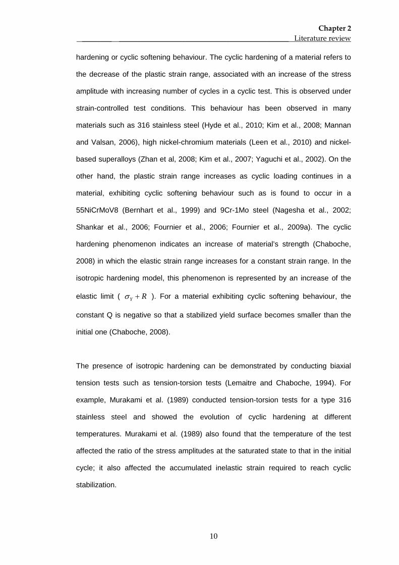
Generally, a material under cyclic loading shows a stabilized stage, in the middle of
its lifetime. However, some materials, such as a martensitic type steels, exhibit an
initially rapid load decrease followed by linear cyclic softening behaviour without the
stabilization of the stress amplitude for a strain-controlled test. In dealing with this
behaviour, Bernhart et al. (1999) employed a two-stage isotropic hardening model,
as given by the following equation:-
)).exp(1).((.)( 21 pbqQpQpR −−+= (2.7)
From the stress amplitude evolution data, the 2Q constant is determined from the
difference between the stress at first cycle and the stress approximately at the end
of the primary load decrease while the 1Q constant is identified from the slope of the
secondary stage, as shown in Figure 2.2. This type of isotropic hardening model
has been used for anisothermal loading conditions (Zhang et al, 2002).
Figure 2.2: Schematical representation of the two-stage cyclic softening model
(Bernhart et al., 1999)
Chapter 2 ________ ______________________________________________ Literature review
12
2.4.2 Kinematic hardening model
The hardening of a material, which occurs due to plastic deformation, can also be
represented by use of a kinematic hardening model. The model uses a different
theoretical approach to that of the isotropic hardening model, in that the yield
surface translates in stress space, rather than expand (Dunne and Petrinic, 2005).
The kinematic hardening parameter χ is a tensor, also called the backstress or rest
stress tensor (Chaboche and Rousselier, 1983), which defines the instantaneous
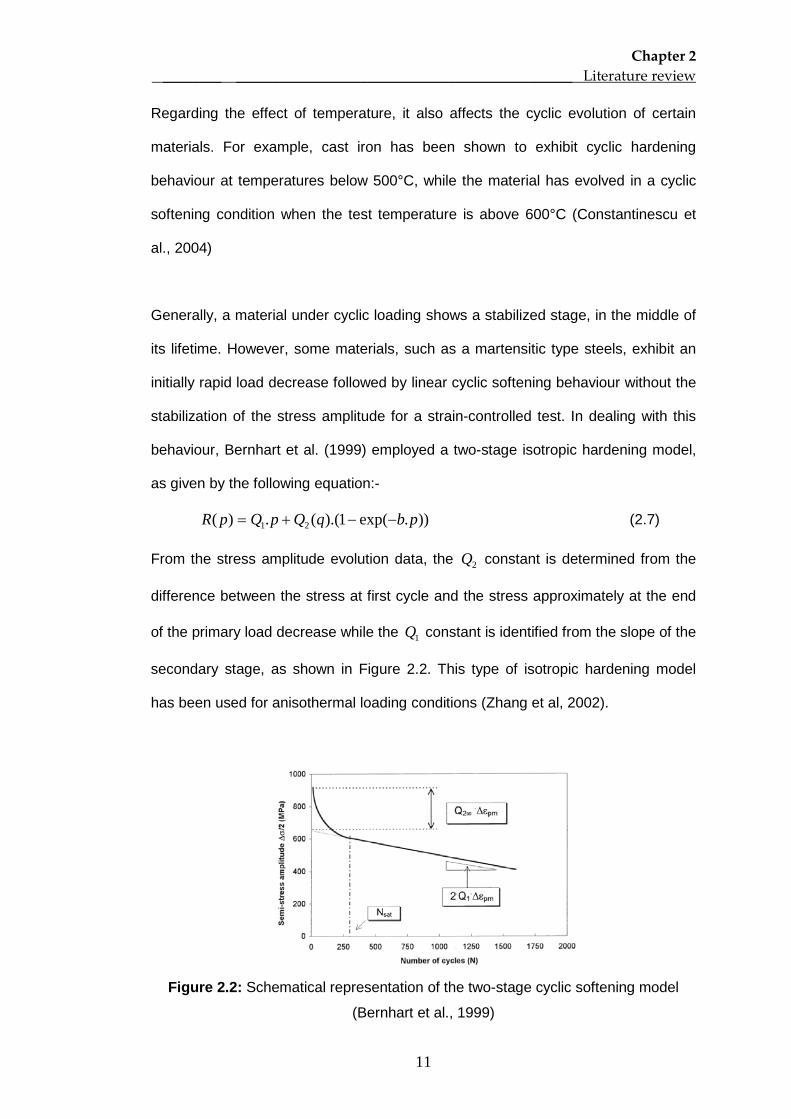
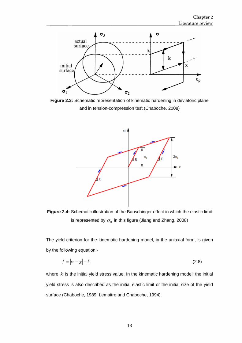
position of the loading surface (Lemaitre and Chaboche, 1994). Figure 2.3 is a
schematic description of the kinematic hardening model in stress space and the
corresponding model in a tension-compression test, in which k represents elastic
limit value.
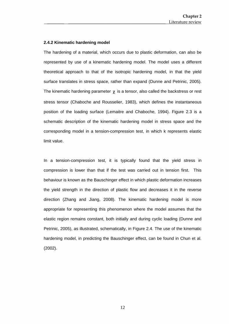
In a tension-compression test, it is typically found that the yield stress in
compression is lower than that if the test was carried out in tension first. This
behaviour is known as the Bauschinger effect in which plastic deformation increases
the yield strength in the direction of plastic flow and decreases it in the reverse
direction (Zhang and Jiang, 2008). The kinematic hardening model is more
appropriate for representing this phenomenon where the model assumes that the
elastic region remains constant, both initially and during cyclic loading (Dunne and
Petrinic, 2005), as illustrated, schematically, in Figure 2.4. The use of the kinematic
hardening model, in predicting the Bauschinger effect, can be found in Chun et al.
(2002).
Chapter 2 ________ ______________________________________________ Literature review
13
Figure 2.3: Schematic representation of kinematic hardening in deviatoric plane
and in tension-compression test (Chaboche, 2008)
Figure 2.4: Schematic illustration of the Bauschinger effect in which the elastic limit
is represented by 0σ in this figure (Jiang and Zhang, 2008)
The yield criterion for the kinematic hardening model, in the uniaxial form, is given
by the following equation:-
kf −−= χσ (2.8)
where k is the initial yield stress value. In the kinematic hardening model, the initial
yield stress is also described as the initial elastic limit or the initial size of the yield
surface (Chaboche, 1989; Lemaitre and Chaboche, 1994).
Chapter 2 ________ ______________________________________________ Literature review
14
The simplest model used to describe kinematic hardening uses a linear relationship
between the change in kinematic hardening and the change in plastic strain. The
linear kinematic hardening model, originally developed by Prager (1949), is given by
the following equation:-
pcεχ 32
= (2.9)
where c is the material constant, which represent the gradient of the linear
relationship (Avanzini, 2008). For the uniaxial loading case, Equation 2.9 is given by
the following:-
pcεχ = (2.10)
where χ represents a scalar variable; the magnitude of χ is 3/2 times the
kinematic hardening tensor parameter (Dunne and Petrinic, 2005). Mroz (1967)
proposed an improvement to the linear kinematic hardening model by introducing a
multilinear model which consists of a multisurface model representing a constant
work hardening modulus in stress space.
Linear strain hardening is rarely observed in the actual cyclic loading tests.
Generally, the stress-strain behaviour obtained from cyclic loading tests is a
nonlinear relationship. The Amstrong-Frederick type kinematic hardening model,
originally developed in 1966, has been used widely to represent this nonlinear
stress-strain relationship. The model introduces a recall term, called dynamic
recovery, into the linear model (Frederick and Armstrong, 2007) which is given by
the following equation:-
pc p χεχ γ−=32
(2.11)
where γ is a material constant. The recall term incorporates a fading memory effect
of the strain path and causes a nonlinear response for the stress-strain behaviour
Chapter 2 ________ ______________________________________________ Literature review
15
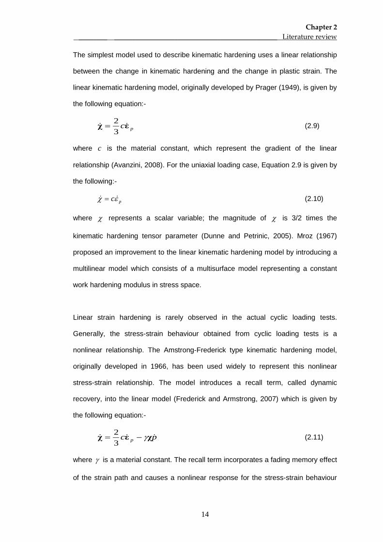
(Bari and Hassan, 2000). For the nonlinear kinematic hardening model of the time-
independent plasticity behaviour, the value of γ/c determines the saturation of
stress value in the plastic region and its combination with the k value represents
the maximum stress for the plasticity test (Dunne and Petrinic, 2005). The saturated
stress is described, schematically, in Figure 2.5.
Figure 2.5: Schematic representation of saturated stress represented by the
nonlinear kinematic hardening model (Dunne and Petrinic, 2005)
The constants in the nonlinear kinematic hardening model are represented by
different equation than that in equation 2.11, as found in Chaboche and Rousselier
(1983), Zhan and Tong (2007) and Gong et al. (2010), for example. The equation is
given as follows:-
−= paC p χεχ
32
(2.12)
where a is the saturation of the stress value in the plastic region, which is identical
to the value of γ/c , and C represents the speed to reach the saturation value,
which is equal to γ . In general, both of the nonlinear kinematic hardening equations
(2.11 and 2.12) are the same, except for the fact that the constants are different in
definition.
Chapter 2 ________ ______________________________________________ Literature review
16
The Amstrong-Frederick hardening relation has been modified by decomposing the
total backstress into a number of additive parts (Jiang and Kurath, 1996). The
reason for the superposition of the kinematic hardening model is to extend the
validity of the kinematic hardening model to a larger domain in stress and strain
(Chaboche and Rousselier, 1983). The model is also intended to describe the
ratchetting behaviour better (Lemaitre and Chaboche, 1994). Thus, the total
backstress χ is given by the following equation:
∑=
=M
ii
1χχ (2.13)
where iχ is a part of the total backstress, i =1,2,…, M and M is the number of the
additive components of the kinematic hardening. The model is usually decomposed
into two or three kinematic variables. However, more variables are sometimes
employed in certain cases, for example, in the study of the ratchetting effect (Bari
and Hassan, 2000), in order to get a better agreement with experimental data. It is
suggested by Chaboche (1986) that the first rule ( 1χ ) should start hardening with a
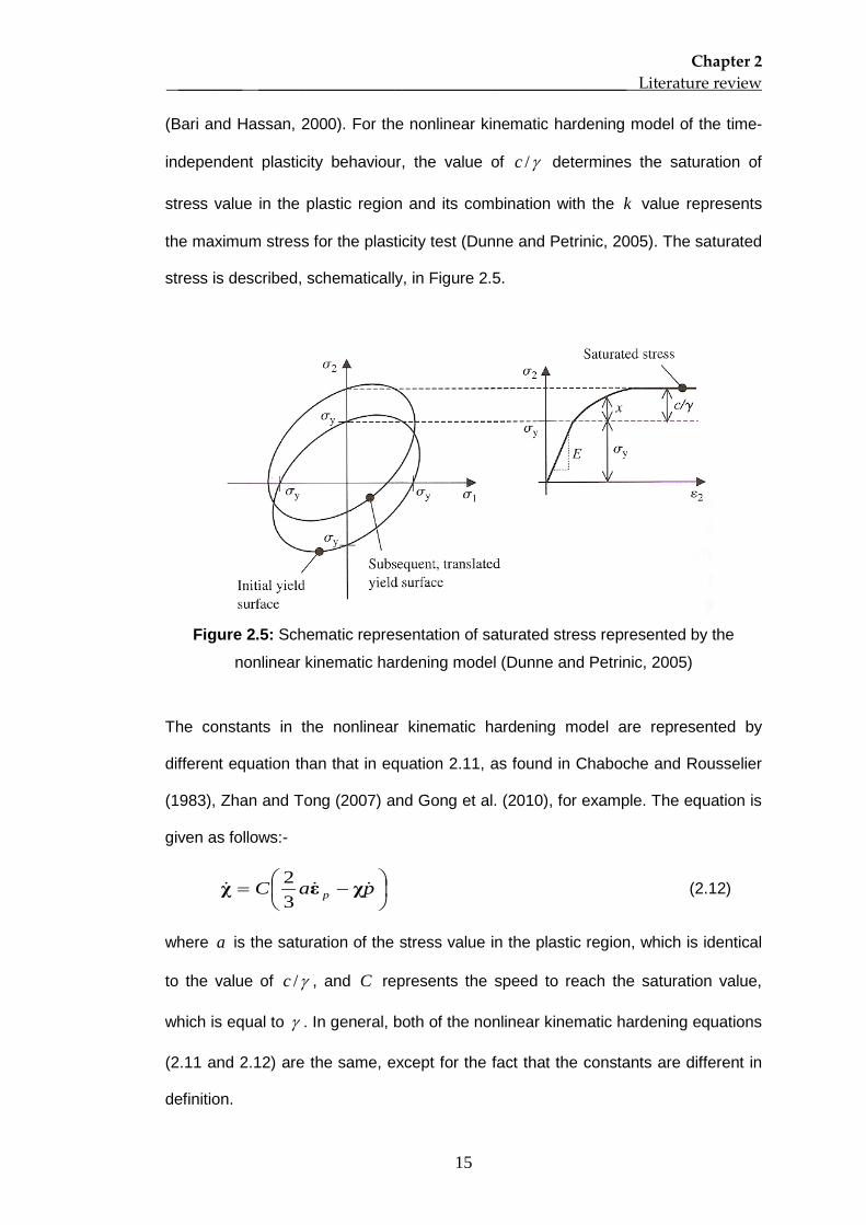
very large modulus and that it stabilizes quickly. For example, the superposition of
three kinematic hardening variables is shown in Figure 2.6.
Figure 2.6: The stress-strain curve obtained from the superposition of three
kinematic hardening variables (Lemaitre and Chaboche, 1994)
Chapter 2 ________ ______________________________________________ Literature review
17
2.4.3 Combined isotropic-kinematic hardening model
Both the cyclic hardening/softening and Bauschinger phenomena are normally
observed in tests of the real material. This observation indicates the requirement to
combine both isotropic and kinematic hardening rules in order to predict the strain
hardening and the cyclic hardening/softening of engineering materials. The yield
criterion of the combined isotropic and kinematic hardening models, in the uniaxial
form, is given by the following equation:-
Rkf −−−= χσ (2.14)
Theoretically, the behaviour of the material with a combined isotropic and kinematic
hardening model will include both the translation and the expansion/contraction of
the yield surface in stress space. An example of the implementation of this
combined model can be found in Zhao et al. (2001). In this paper, the author used a
time independent cyclic plasticity model combined with isotropic hardening and two
nonlinear kinematic hardening rules, to predict the behaviour of a nickel base
superalloy, at 300°C.
2.5 Time-dependent cyclic plasticity
The repeated loading of engineering components at high temperature may involve
both plasticity and creep behaviour. The constitutive model for this condition is
known as a time-dependent or a rate-dependent plasticity in which the plastic strain
and the creep strain contribute to the total strain value.
2.5.1 Uncoupled elastoplasticity-creep
Conventionally, the creep (time-dependent) and the plasticity (time-independent)
behaviour are modelled by an uncoupled elastic-plasticity-creep model. In the
model, the stress-strain behaviour is represented by a creep model such as the
Chapter 2 ________ ______________________________________________ Literature review
18
Norton’s law and by a typical plasticity model such as the isotropic and kinematic
hardening models. For example, Shang et al. (2006) used the model to represent
the behaviour of superplastic forming dies. The constants for the selected creep and
plasticity models are determined separately in a constant loading test and in cyclic
loading tests, respectively, and there is no interaction assumed to occur between
those constants in the creep and plasticity equations. In certain conditions,
particularly for cyclic creep (ratchetting effect) and creep-plasticity interaction, the
combination of the plasticity and creep equations give unsatisfactory results when
compared to experimental data (Krempl, 2000). Thus, a viscoplasticity model has
been used more frequently than the uncoupled elastic-plasticity-creep model to
describe time-dependent plasticity behaviour at high temperature.
2.5.2 Unified viscoplasticity model
According to Lemaitre (2001), the viscoplasticity model refers to the mechanical
response of materials in plastic condition which exhibits time dependent effect
represented by a viscosity function. A well known viscoplasticity model is the unified
viscoplasticity model proposed by Chaboche (Chaboche and Rousselier, 1983). The
model is known as the “unified” viscoplasticity model for two reasons (Chaboche,
1989). Firstly, the plastic and the creep strains are represented simultaneously by
one parameter and these strains are called the viscoplastic strain. Consequently,
the strain does not exhibit a discontinuity under different types of loading. Secondly,
the same hardening rules as the time independent plasticity rule are employed in
the viscoplasticity model.
The viscoplastic strain rate of the model, in the uniaxial form, is given by the
following equations:-
Chapter 2 ________ ______________________________________________ Literature review
19
)sgn( χσε −=n
p Zf
(2.15)
where:
<−=>
=0,1
0,00,1
)sgn(x
xx
x and
<≥
=0,00,
xxx
x (2.16)
Rkf −−−= χσ (2.17)
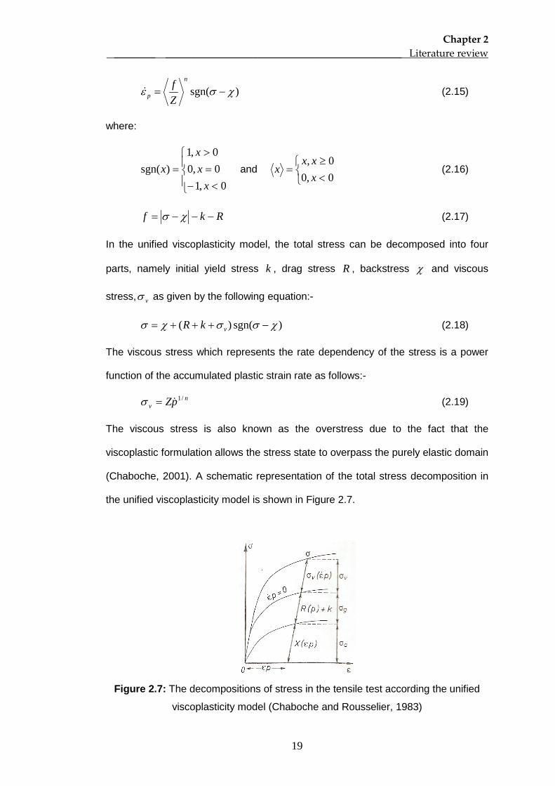
In the unified viscoplasticity model, the total stress can be decomposed into four
parts, namely initial yield stress k , drag stress R , backstress χ and viscous
stress, vσ as given by the following equation:-
)sgn()( χσσχσ −+++= vkR (2.18)
The viscous stress which represents the rate dependency of the stress is a power
function of the accumulated plastic strain rate as follows:-
nv pZ /1=σ (2.19)
The viscous stress is also known as the overstress due to the fact that the
viscoplastic formulation allows the stress state to overpass the purely elastic domain
(Chaboche, 2001). A schematic representation of the total stress decomposition in
the unified viscoplasticity model is shown in Figure 2.7.
Figure 2.7: The decompositions of stress in the tensile test according the unified
viscoplasticity model (Chaboche and Rousselier, 1983)
Chapter 2 ________ ______________________________________________ Literature review
20
The unified viscoplasticity model has been used by Tong and his co-workers to
predict the stress-strain behaviour of a nickel-based superalloy. For example, Zhao
et al. (2001) developed the unified model to predict the stabilized cyclic loops of a
nickel base superalloy at various strain ranges and at high temperatures. At the
beginning of the work, only one strain rate was used in the study. An optimisation
method was used to improve the initially determined parameters by minimizing the
difference between the predicted and the experimental stress values. The
optimisation method was further improved by considering several types of test data
in the optimisation process such as monotonic, cyclic, relaxation and creep test data
(Tong and Vermeulen, 2003; and Tong et al., 2004) and this process resulted in
better predictions for the cyclic and creep tests by using only a single inelastic strain
variable within the model. Additional terms can be included in the model such as a
static recovery term (Zhan and Tong, 2007) and a plastic strain memory term (Zhan
et al., 2008) in order to improve the model’s prediction for more complex stress-
strain behaviour. It can be seen from the works of Tong and his co-workers that the
viscoplasticity model for the nickel-based superalloy has been developed in several
stages, starting from a simple model, and the optimisation program has been used
to determine the material constants.
Yaguchi and Takahashi (2000) used a unified viscoplastic model to represent the
cyclic behaviour of modified 9Cr-1Mo steel under temperatures between 200 and
600°C. In the proposed model, the applied stress has been divided into three
components; a back stress, an effective stress and an aging stress. The aging
stress in the model is similar to the isotropic hardening variable, but is represented
by different equations. The cyclic softening behaviour of the modified 9Cr-1Mo steel
is represented by a modified kinematic hardening equation. The constants of the
Chapter 2 ________ ______________________________________________ Literature review
21
model were determined by a step-by-step procedure and it involves a trial-and-error
method. The model shows a good capability to describe the inelastic behaviour of
modified 9Cr-1Mo steel under monotonic tension, stress relaxation, creep and
anisothermal cyclic deformation. In order to improve the ratchetting behaviour
prediction, Yaguchi and Takahashi (2005) modified their model by using the Ohno-
Wang kinematic hardening rules. Koo and Lee (2007) also investigated the
ratchetting behaviour of the modified 9Cr-1Mo steel at 600°C; however, a rate-
independent model incorporating a kinematic hardening rule with three-decomposed
rules and an isotropic hardening rule was used in their work.
In general, the phenomenologically based model is capable of predicting the
behaviour of undamaged material for which the stress-strain prediction of the model
is true up to a certain number of cycles and normally covers the majority of life
cycles. In order to simulate the behaviour of a material for the whole of fatigue
process, the material constitutive model could be combined with continuum damage
mechanics theory. The damage mechanics theory enables the modelling of the
material’s strength degradation and the often rapid collapse of the specimen (Oller
et al., 2005). The fatigue damage evolution is described in terms of the number of
cycles and it may depend on several variables such as stress, plastic strain,
damage variable, D , temperature or hardening variables (Shang and Yao, 1999)
For higher temperature applications, the creep-fatigue damage may be combined to
provide a unified viscoplasticity model which can predict the failure of the specimen.
The evolution of the combined damage approach is described by the following
equation (Chaboche and Gallerneau, 2001):-
dNTDfdtTDfdD FC ),,,(),,( max σσσ += (2.20)
Chapter 2 ________ ______________________________________________ Literature review
22
where the evolution of creep damage is based on the time evolution while the
fatigue damage evolution is based on the evolution of the number of cycles. The
model has been successfully applied to a nickel based superalloy (Yeom et al.,
2007, El Gharad et al., 2006) and a single crystal (Dunne and Hayhurst, 1992a;
Dunne and Hayhurst, 1992b). However, the inclusion of a creep-damage model into
the constitutive equation requires many types of test loading configurations to be
implemented and thus many specimens are required in the testing program (Dunne
et al., 1992).
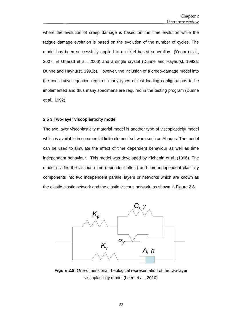
2.5 3 Two-layer viscoplasticity model
The two layer viscoplasticity material model is another type of viscoplasticity model
which is available in commercial finite element software such as Abaqus. The model
can be used to simulate the effect of time dependent behaviour as well as time
independent behaviour. This model was developed by Kichenin et al. (1996). The
model divides the viscous (time dependent effect) and time independent plasticity
components into two independent parallel layers or networks which are known as
the elastic-plastic network and the elastic-viscous network, as shown in Figure 2.8.
Figure 2.8: One-dimensional rheological representation of the two-layer
viscoplasticity model (Leen et al., 2010)
Chapter 2 ________ ______________________________________________ Literature review
23
The interactions of elastic-plastic and elastic-viscous networks are controlled by the
user-specified ratio, f . The parameter is defined by the following equation:-
vp
v
KKK
f+
= (2.21)
where vK and pK are the elastic modulus in the viscous and the plastic networks,
respectively. The f value lies in the range 0 and 1 in which a value close to 1
indicates a high contribution of elastic viscous network. In isothermal conditions, the
total strain is decomposed into elastic, eε , plastic, pε and viscous, vε , strain
components, as follows:-
vpe ff εεεε +−+= )1( (2.22)
The total stress of the model is divided into two different stresses, i.e., pσ and vσ ,
which control the evolution of plasticity and viscous effects in each network,
respectively.
General plasticity and creep models can be implemented in the two-layer
viscoplasticity model. For example, Figiel and Gunther (2008) used the nonlinear
isotropic and the kinematic hardening model in the elastic-plastic network while the
Norton power law model was selected for the elastic-viscous network. The model
constants in the study were obtained by fitting the results of finite element
simulations to quasi-static tensile and relaxation experimental tests carried out at
various temperatures. Similar plasticity and creep models were chosen by Leen et
al. (2010) which include combined isotropic-kinematic hardening plasticity and
power law creep model to be used in the two-layer viscoplasticity model. Leen et al.
(2010) determined the material constants for the combined isotropic-kinematic
hardening by conducting isothermal cyclic tests while the creep model constants
were identified from isothermal stress relaxation tests carried out at various
Chapter 2 ________ ______________________________________________ Literature review
24
temperatures. Finally, the user-specified ratio, f , is identified by a fitting process
which compares finite element predictions with experimental stress relaxation
results.
The two-layer viscoplasticity model has been derived for several materials in order
to represent the stress-strain behaviour, particularly for high temperature
application. Charkaluk et al. (2002) used the two-layer viscoplasticity model to
represent the cyclic behaviour of a cast iron, which is used in exhaust manifold
structures. Leen et al. (2010) characterized the cyclic elastic-plastic-creep behaviour
of a high nickel-chromium material (XN40F) which is used in superplastic forming
tools at temperatures in the range 20°C to 900°C. The model has also been used to
analyse polyelectrolyte membranes in fuel cells (Solasi et al. (2008). In earlier work
on this model carried out by Kichenin et al. (1996), the nonlinear visco-elasticity
behaviour of polyethylene was represented.
2.6 Material behaviour under TMF conditions
A great deal of research has been carried out in order to characterize the
thermomechanical behaviour of engineering materials, using types of material
models. For example, the two-layer model and the unified viscoplasticity model
have been used to predict the behaviour of an exhaust manifold under
thermomechanical fatigue conditions; both models exhibited similar mechanical
responses (Charkaluk et al., 2002). Yaguchi et al. (2002) applied the unified
viscoplasticity model to predict the anisothermal behaviour of a nickel-based
superalloy between 450 and 950°C. The two-layer viscoplasticity model has also
been successfully used to predict the behaviour of a high nickel-chromium material
used in a superplastic forming process (Leen et al., 2010). Minichmayr et al. (2008)
used the nonlinear kinematic hardening model and the Norton creep model to
Chapter 2 ________ ______________________________________________ Literature review
25
describe the behaviour of aluminium-silicon cast alloy, machined from cylinder
heads of combustion engines.
The constants for the material behaviour model in anisothermal conditions are
commonly developed by determining material model constants under isothermal
conditions for several temperatures in a specified temperature range. For example,
Hyde et al. (2010) developed a unified Chaboche viscoplasticity model for a 316
stainless steel using isothermal strain-controlled test data with ±0.3% strain
amplitude for temperatures in the range 300 and 600°C. The model gives good
predictions when compared with experimental in-phase and out-of-phase
thermomechanical fatigue test results even though the TMF tests were subjected to
a higher mechanical strain range. The same approach was used by Leen et al.
(2010) and Yaguchi et al. (2002) to characterize the thermomechanical fatigue
behaviour of materials with a two-layer viscoplasticity and a unified viscoplasticity
model, respectively.
The behaviour of P91 steel under thermomechanical fatigue loading conditions was
studied by Okrajni et al. (2008). In the study, out-of-phase TMF loading was applied
to a hollow specimen subjected to temperatures with the range 200 and 450°C. A
mathematical model was developed, based on a low-cycle isothermal fatigue tests,
and the top and bottom values of stress and strain were used in the model. The
model gives good predictions when compared with the experimental results, as
shown in Figure 2.9(a). However, only the behaviour of the steel at the sample size,
was included in this study. The thermomechanical behaviour of another power plant
material, ie, a P23 steel, was modelled by Hartrott et al. (2009) using a unified
viscoplasticity model, which is a phenomenological-based model, and the model’s
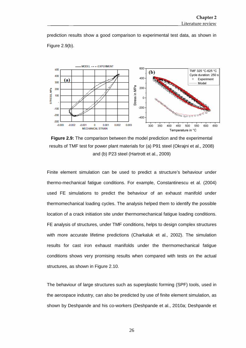
Chapter 2 ________ ______________________________________________ Literature review
26
prediction results show a good comparison to experimental test data, as shown in
Figure 2.9(b).
Figure 2.9: The comparison between the model prediction and the experimental
results of TMF test for power plant materials for (a) P91 steel (Okrajni et al., 2008)
and (b) P23 steel (Hartrott et al., 2009)
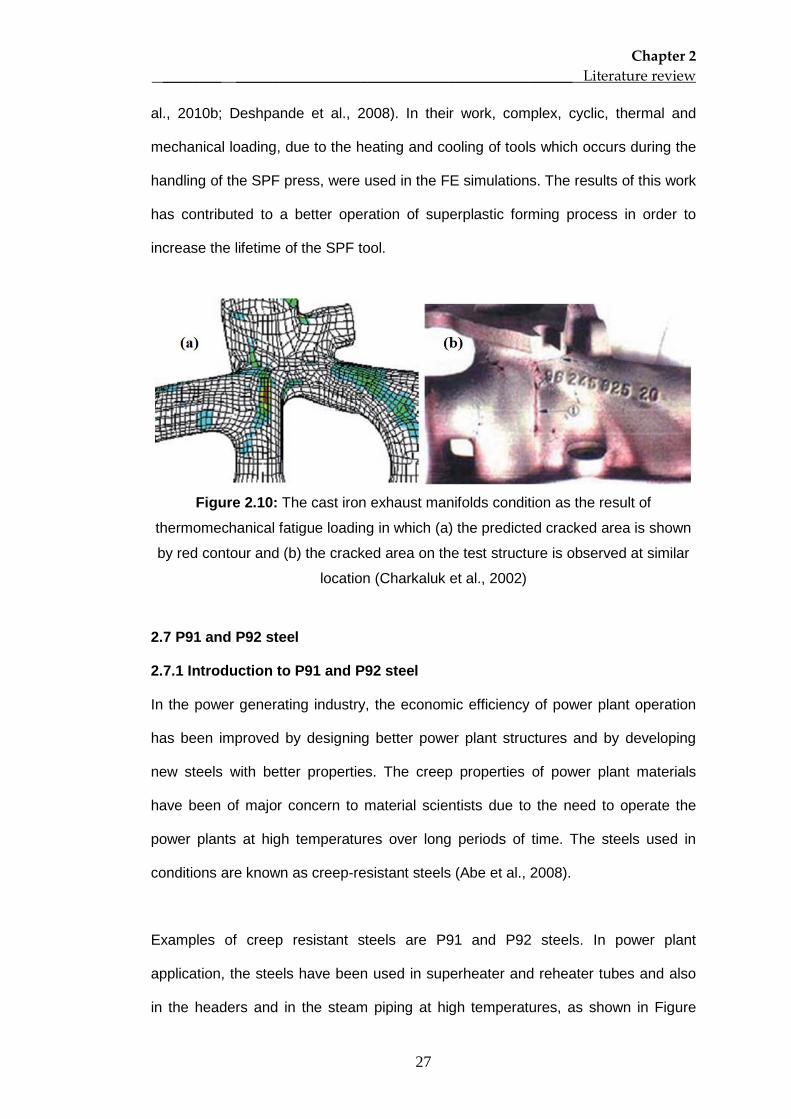
Finite element simulation can be used to predict a structure’s behaviour under
thermo-mechanical fatigue conditions. For example, Constantinescu et al. (2004)
used FE simulations to predict the behaviour of an exhaust manifold under
thermomechanical loading cycles. The analysis helped them to identify the possible
location of a crack initiation site under thermomechanical fatigue loading conditions.
FE analysis of structures, under TMF conditions, helps to design complex structures
with more accurate lifetime predictions (Charkaluk et al., 2002). The simulation
results for cast iron exhaust manifolds under the thermomechanical fatigue
conditions shows very promising results when compared with tests on the actual
structures, as shown in Figure 2.10.
The behaviour of large structures such as superplastic forming (SPF) tools, used in
the aerospace industry, can also be predicted by use of finite element simulation, as
shown by Deshpande and his co-workers (Deshpande et al., 2010a; Deshpande et
Chapter 2 ________ ______________________________________________ Literature review
27
al., 2010b; Deshpande et al., 2008). In their work, complex, cyclic, thermal and
mechanical loading, due to the heating and cooling of tools which occurs during the
handling of the SPF press, were used in the FE simulations. The results of this work
has contributed to a better operation of superplastic forming process in order to
increase the lifetime of the SPF tool.
Figure 2.10: The cast iron exhaust manifolds condition as the result of
thermomechanical fatigue loading in which (a) the predicted cracked area is shown
by red contour and (b) the cracked area on the test structure is observed at similar
location (Charkaluk et al., 2002)
2.7 P91 and P92 steel
2.7.1 Introduction to P91 and P92 steel
In the power generating industry, the economic efficiency of power plant operation
has been improved by designing better power plant structures and by developing
new steels with better properties. The creep properties of power plant materials
have been of major concern to material scientists due to the need to operate the
power plants at high temperatures over long periods of time. The steels used in
conditions are known as creep-resistant steels (Abe et al., 2008).
Examples of creep resistant steels are P91 and P92 steels. In power plant
application, the steels have been used in superheater and reheater tubes and also
in the headers and in the steam piping at high temperatures, as shown in Figure
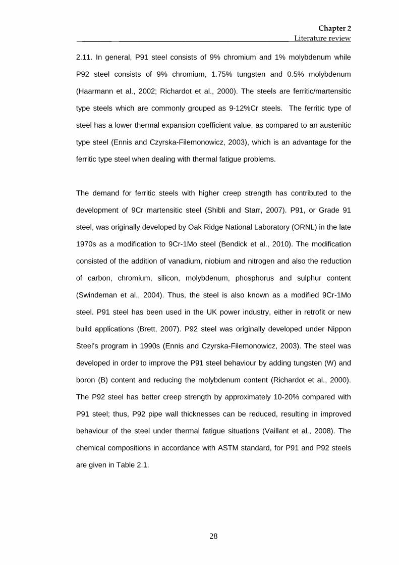
Chapter 2 ________ ______________________________________________ Literature review
28
2.11. In general, P91 steel consists of 9% chromium and 1% molybdenum while
P92 steel consists of 9% chromium, 1.75% tungsten and 0.5% molybdenum
(Haarmann et al., 2002; Richardot et al., 2000). The steels are ferritic/martensitic
type steels which are commonly grouped as 9-12%Cr steels. The ferritic type of
steel has a lower thermal expansion coefficient value, as compared to an austenitic
type steel (Ennis and Czyrska-Filemonowicz, 2003), which is an advantage for the
ferritic type steel when dealing with thermal fatigue problems.
The demand for ferritic steels with higher creep strength has contributed to the
development of 9Cr martensitic steel (Shibli and Starr, 2007). P91, or Grade 91
steel, was originally developed by Oak Ridge National Laboratory (ORNL) in the late
1970s as a modification to 9Cr-1Mo steel (Bendick et al., 2010). The modification
consisted of the addition of vanadium, niobium and nitrogen and also the reduction
of carbon, chromium, silicon, molybdenum, phosphorus and sulphur content
(Swindeman et al., 2004). Thus, the steel is also known as a modified 9Cr-1Mo
steel. P91 steel has been used in the UK power industry, either in retrofit or new
build applications (Brett, 2007). P92 steel was originally developed under Nippon
Steel’s program in 1990s (Ennis and Czyrska-Filemonowicz, 2003). The steel was
developed in order to improve the P91 steel behaviour by adding tungsten (W) and
boron (B) content and reducing the molybdenum content (Richardot et al., 2000).
The P92 steel has better creep strength by approximately 10-20% compared with
P91 steel; thus, P92 pipe wall thicknesses can be reduced, resulting in improved
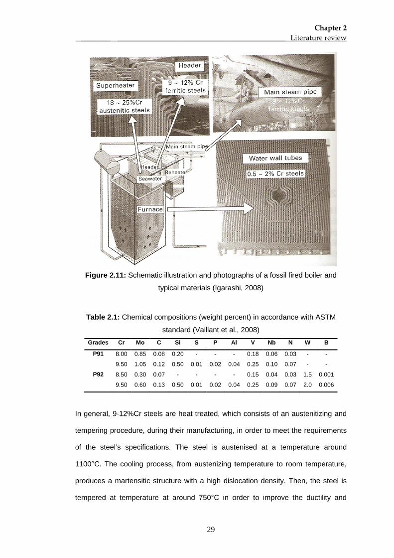
behaviour of the steel under thermal fatigue situations (Vaillant et al., 2008). The
chemical compositions in accordance with ASTM standard, for P91 and P92 steels
are given in Table 2.1.
Chapter 2 ________ ______________________________________________ Literature review
29
Figure 2.11: Schematic illustration and photographs of a fossil fired boiler and
typical materials (Igarashi, 2008)
Table 2.1: Chemical compositions (weight percent) in accordance with ASTM
standard (Vaillant et al., 2008)
Grades Cr Mo C Si S P Al V Nb N W B
P91 8.00 0.85 0.08 0.20 - - - 0.18 0.06 0.03 - -
9.50 1.05 0.12 0.50 0.01 0.02 0.04 0.25 0.10 0.07 - -
P92 8.50 0.30 0.07 - - - - 0.15 0.04 0.03 1.5 0.001
9.50 0.60 0.13 0.50 0.01 0.02 0.04 0.25 0.09 0.07 2.0 0.006
In general, 9-12%Cr steels are heat treated, which consists of an austenitizing and
tempering procedure, during their manufacturing, in order to meet the requirements
of the steel’s specifications. The steel is austenised at a temperature around
1100°C. The cooling process, from austenizing temperature to room temperature,
produces a martensitic structure with a high dislocation density. Then, the steel is
tempered at temperature at around 750°C in order to improve the ductility and
Chapter 2 ________ ______________________________________________ Literature review
30
impact strength. Subgrains and dislocation networks are formed during tempering
(Maruyama et al., 2001; Ennis and Czyrska-Filemonowicz, 2003). Different
temperatures and periods of heat treatments are reported in the literature for 9-
12%Cr steels, as listed in Fournier et al. (2009b). The different parameters used for
the austenitizing and tempering processes can affect the microstructure of the
steels. For example, selecting a high austenitising temperature results in an
increase in the lath width and an increase in the prior austenite grain size (Ennis
and Czyrska-Filemonowicz, 2003). The variation in heat treatment can also result in
slight differences in mechanical properties.
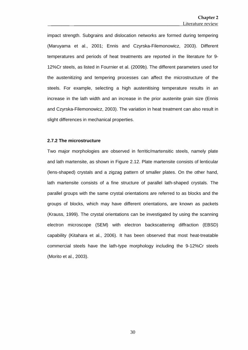
2.7.2 The microstructure
Two major morphologies are observed in ferritic/martensitic steels, namely plate
and lath martensite, as shown in Figure 2.12. Plate martensite consists of lenticular
(lens-shaped) crystals and a zigzag pattern of smaller plates. On the other hand,
lath martensite consists of a fine structure of parallel lath-shaped crystals. The
parallel groups with the same crystal orientations are referred to as blocks and the
groups of blocks, which may have different orientations, are known as packets
(Krauss, 1999). The crystal orientations can be investigated by using the scanning
electron microscope (SEM) with electron backscattering diffraction (EBSD)
capability (Kitahara et al., 2006). It has been observed that most heat-treatable
commercial steels have the lath-type morphology including the 9-12%Cr steels
(Morito et al., 2003).
Chapter 2 ________ ______________________________________________ Literature review
31
Figure 2.12: The example of microstructure of (a) lath martensite in a 4140 steel
and (b) plate martensite in the Fe-1.86%Cr alloy (Krauss. 1999)
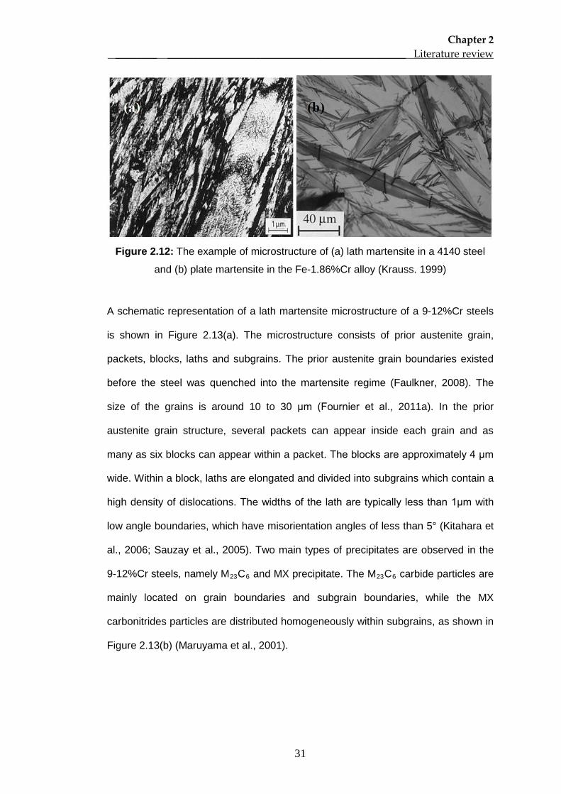
A schematic representation of a lath martensite microstructure of a 9-12%Cr steels
is shown in Figure 2.13(a). The microstructure consists of prior austenite grain,
packets, blocks, laths and subgrains. The prior austenite grain boundaries existed
before the steel was quenched into the martensite regime (Faulkner, 2008). The
size of the grains is around 10 to 30 μm (Fournier et al., 2011a). In the prior
austenite grain structure, several packets can appear inside each grain and as
many as six blocks can appear within a packet. The blocks are approximately 4 μm
wide. Within a block, laths are elongated and divided into subgrains which contain a
high density of dislocations. The widths of the lath are typically less than 1μm with
low angle boundaries, which have misorientation angles of less than 5° (Kitahara et
al., 2006; Sauzay et al., 2005). Two main types of precipitates are observed in the
9-12%Cr steels, namely M23C6 and MX precipitate. The M23C6
carbide particles are
mainly located on grain boundaries and subgrain boundaries, while the MX
carbonitrides particles are distributed homogeneously within subgrains, as shown in
Figure 2.13(b) (Maruyama et al., 2001).
Chapter 2 ________ ______________________________________________ Literature review
32
Figure 2.13: The schematic of (a) lath martensite microstructure (Fournier et al.,
2009b) and (b) precipitates (Maruyama et al., 2001) of 9-12% Cr steels
The microstructure of martensitic steels contributes to the strength of the material.
For example, the subgrain boundaries, the dislocations and the precipitates
characteristics influence the deformation of the steel. The subgrain boundaries
become obstacles to dislocation motion during inelastic deformation such as that
which occurs in creep and fatigue conditions (Kostka et al., 2007). The precipitates
contribute to the creep strength of the steel by pinning grain boundaries so that the
grain size is stabilized during high temperature application (Faulkner, 2008). Smaller
precipitates, distributed within subgrains, may act as obstacles to the mobility of the
subgrain dislocations (Fournier et al., 2011a).
2.7.3 The microstructural evolution under cyclic loading test
Comparisons between as-received specimens and those that have failed under
cyclic loading conditions for 9-12%Cr steels, reveals that an increase of subgrain
size and a decrease of dislocation density has occurred (Armas et al., 2004; Dubey
et al., 2005; Fournier et al., 2009b). The microstructural evolution in the steels have
been investigated using transmission electron microscopy (TEM) and examples of
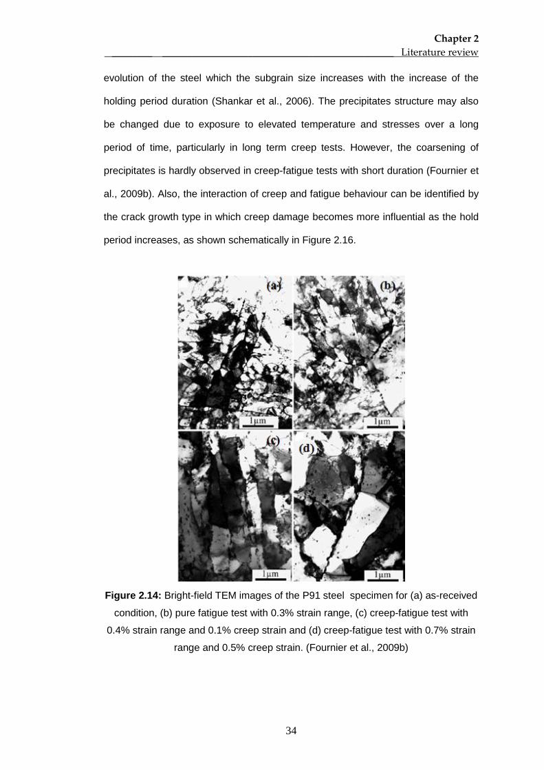
the subgrain coarsening which occurs are shown in Figure 2.14. Cyclic inelastic
Chapter 2 ________ ______________________________________________ Literature review
33
deformation leads to the coarsening of the subgrains where experimental results
show that the subgrains sizes increase with an increase in the applied plastic strain.
It has been found that microstructural coarsening, under cyclic loading, occurs on a
subgrain scale without modifying the block of laths (Fournier et al., 2009b; Kimura et
al., 2006). Also, the blocks are more homogeneous after cyclic loading which may
indicate the disappearance of subgrain boundaries. This observation may be a
result of the limitation of scanning electron microscopy (SEM) in observing the
microstructural evolution of the steel, due to the fact that SEM can only observe
high angle boundaries, which include prior austenite grains, packets and blocks
(Kimura et al., 2006).
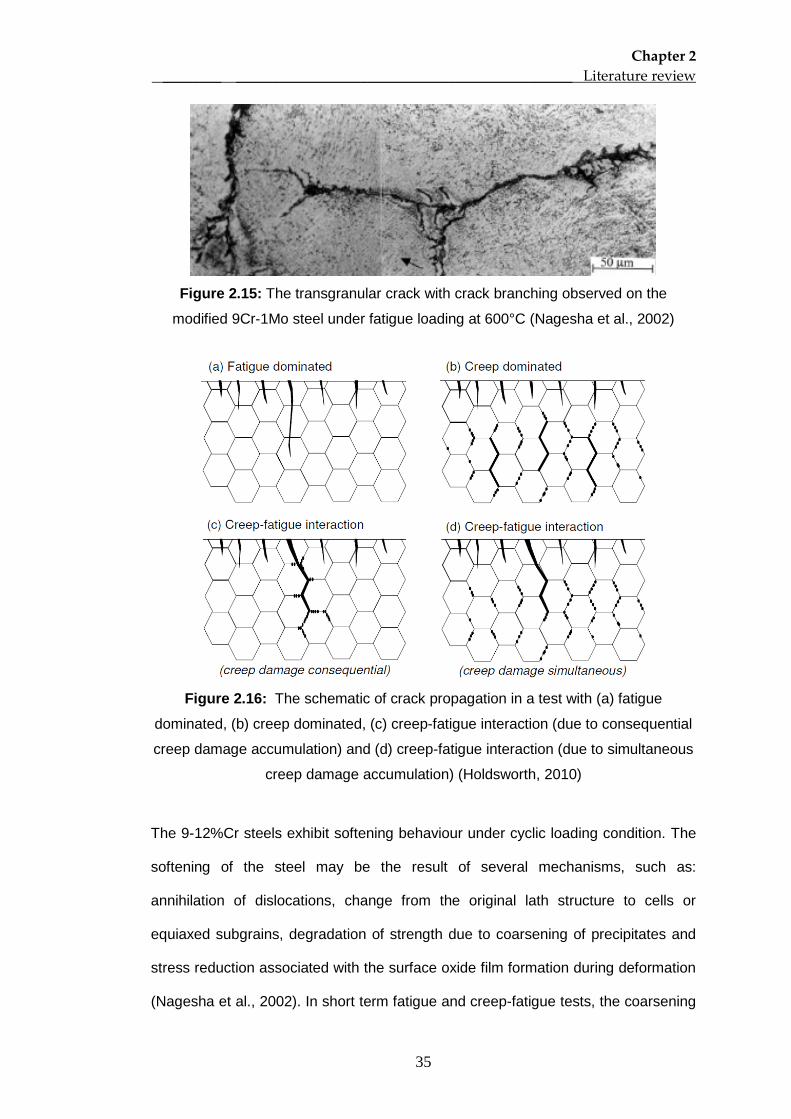
Scanning electron microscope and optical microscopy have been used to study
crack initiation and propagation modes in 9-12%Cr steels under cyclic loading
conditions. The microstructural observation of the fatigue specimen of the modified
9Cr-1Mo steel, such as a test with a strain rate of 3x10⁻³ s-1
, has revealed a
transgranular crack type with crack branching, as shown in Figure 2.15. It has also
been found that the oxidation may influence the crack initiation and propagation,
particularly at low strain amplitudes (e.g. ±0.25%) and high temperatures (Nagesha
et al., 2002; Shankar et al., 2006).
The interaction between creep and fatigue behaviours within cyclic loading tests
produces greater microstructural evolutions than occur in pure fatigue tests. For
example, from the Figure 2.14(d), the subgrain size of the creep-fatigue tests
specimens are up to 3 times greater after the test while the coarsening of the
subgrains in pure fatigue tests show lower increases of subgrains with them being
up to 2 times greater than those in the as-received specimens (Fournier et al.,
2009b). This observation indicates the test duration effect on the microstructural
Chapter 2 ________ ______________________________________________ Literature review
34
evolution of the steel which the subgrain size increases with the increase of the
holding period duration (Shankar et al., 2006). The precipitates structure may also
be changed due to exposure to elevated temperature and stresses over a long
period of time, particularly in long term creep tests. However, the coarsening of
precipitates is hardly observed in creep-fatigue tests with short duration (Fournier et
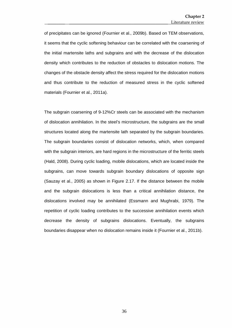
al., 2009b). Also, the interaction of creep and fatigue behaviour can be identified by
the crack growth type in which creep damage becomes more influential as the hold
period increases, as shown schematically in Figure 2.16.
Figure 2.14: Bright-field TEM images of the P91 steel specimen for (a) as-received
condition, (b) pure fatigue test with 0.3% strain range, (c) creep-fatigue test with
0.4% strain range and 0.1% creep strain and (d) creep-fatigue test with 0.7% strain
range and 0.5% creep strain. (Fournier et al., 2009b)
Chapter 2 ________ ______________________________________________ Literature review
35
Figure 2.15: The transgranular crack with crack branching observed on the
modified 9Cr-1Mo steel under fatigue loading at 600°C (Nagesha et al., 2002)
Figure 2.16: The schematic of crack propagation in a test with (a) fatigue
dominated, (b) creep dominated, (c) creep-fatigue interaction (due to consequential
creep damage accumulation) and (d) creep-fatigue interaction (due to simultaneous
creep damage accumulation) (Holdsworth, 2010)
The 9-12%Cr steels exhibit softening behaviour under cyclic loading condition. The
softening of the steel may be the result of several mechanisms, such as:
annihilation of dislocations, change from the original lath structure to cells or
equiaxed subgrains, degradation of strength due to coarsening of precipitates and
stress reduction associated with the surface oxide film formation during deformation
(Nagesha et al., 2002). In short term fatigue and creep-fatigue tests, the coarsening
Chapter 2 ________ ______________________________________________ Literature review
36
of precipitates can be ignored (Fournier et al., 2009b). Based on TEM observations,
it seems that the cyclic softening behaviour can be correlated with the coarsening of
the initial martensite laths and subgrains and with the decrease of the dislocation
density which contributes to the reduction of obstacles to dislocation motions. The
changes of the obstacle density affect the stress required for the dislocation motions
and thus contribute to the reduction of measured stress in the cyclic softened
materials (Fournier et al., 2011a).
The subgrain coarsening of 9-12%Cr steels can be associated with the mechanism
of dislocation annihilation. In the steel’s microstructure, the subgrains are the small
structures located along the martensite lath separated by the subgrain boundaries.
The subgrain boundaries consist of dislocation networks, which, when compared
with the subgrain interiors, are hard regions in the microstructure of the ferritic steels
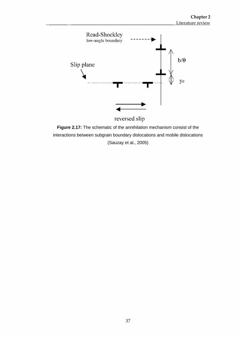
(Hald, 2008). During cyclic loading, mobile dislocations, which are located inside the
subgrains, can move towards subgrain boundary dislocations of opposite sign
(Sauzay et al., 2005) as shown in Figure 2.17. If the distance between the mobile
and the subgrain dislocations is less than a critical annihilation distance, the
dislocations involved may be annihilated (Essmann and Mughrabi, 1979). The
repetition of cyclic loading contributes to the successive annihilation events which
decrease the density of subgrains dislocations. Eventually, the subgrains
boundaries disappear when no dislocation remains inside it (Fournier et al., 2011b).
Chapter 2 ________ ______________________________________________ Literature review
37
Figure 2.17: The schematic of the annihilation mechanism consist of the
interactions between subgrain boundary dislocations and mobile dislocations
(Sauzay et al., 2005)
Chapter 3 _____________ Experimental work
38
Chapter 3 – Experimental work
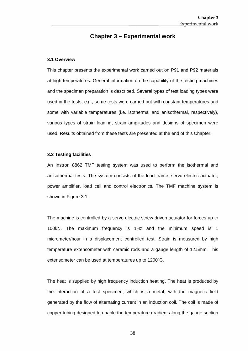
3.1 Overview
This chapter presents the experimental work carried out on P91 and P92 materials
at high temperatures. General information on the capability of the testing machines
and the specimen preparation is described. Several types of test loading types were
used in the tests, e.g., some tests were carried out with constant temperatures and
some with variable temperatures (i.e. isothermal and anisothermal, respectively),
various types of strain loading, strain amplitudes and designs of specimen were
used. Results obtained from these tests are presented at the end of this Chapter.
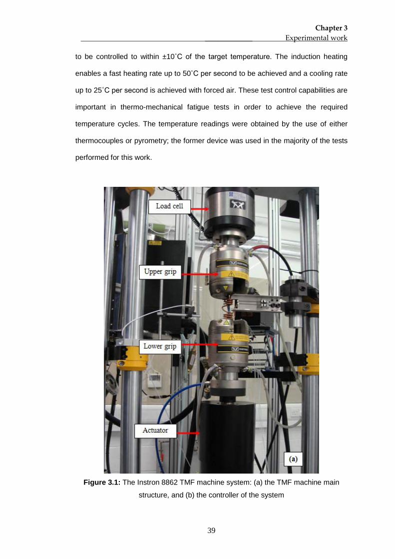
3.2 Testing facilities
An Instron 8862 TMF testing system was used to perform the isothermal and
anisothermal tests. The system consists of the load frame, servo electric actuator,
power amplifier, load cell and control electronics. The TMF machine system is
shown in Figure 3.1.
The machine is controlled by a servo electric screw driven actuator for forces up to
100kN. The maximum frequency is 1Hz and the minimum speed is 1
micrometer/hour in a displacement controlled test. Strain is measured by high
temperature extensometer with ceramic rods and a gauge length of 12.5mm. This
extensometer can be used at temperatures up to 1200˚C.
The heat is supplied by high frequency induction heating. The heat is produced by
the interaction of a test specimen, which is a metal, with the magnetic field
generated by the flow of alternating current in an induction coil. The coil is made of
copper tubing designed to enable the temperature gradient along the gauge section
Chapter 3 _____________ Experimental work
39
to be controlled to within ±10˚C of the target temperature. The induction heating
enables a fast heating rate up to 50˚C per second to be achieved and a cooling rate
up to 25˚C per second is achieved with forced air. These test control capabilities are
important in thermo-mechanical fatigue tests in order to achieve the required
temperature cycles. The temperature readings were obtained by the use of either
thermocouples or pyrometry; the former device was used in the majority of the tests
performed for this work.
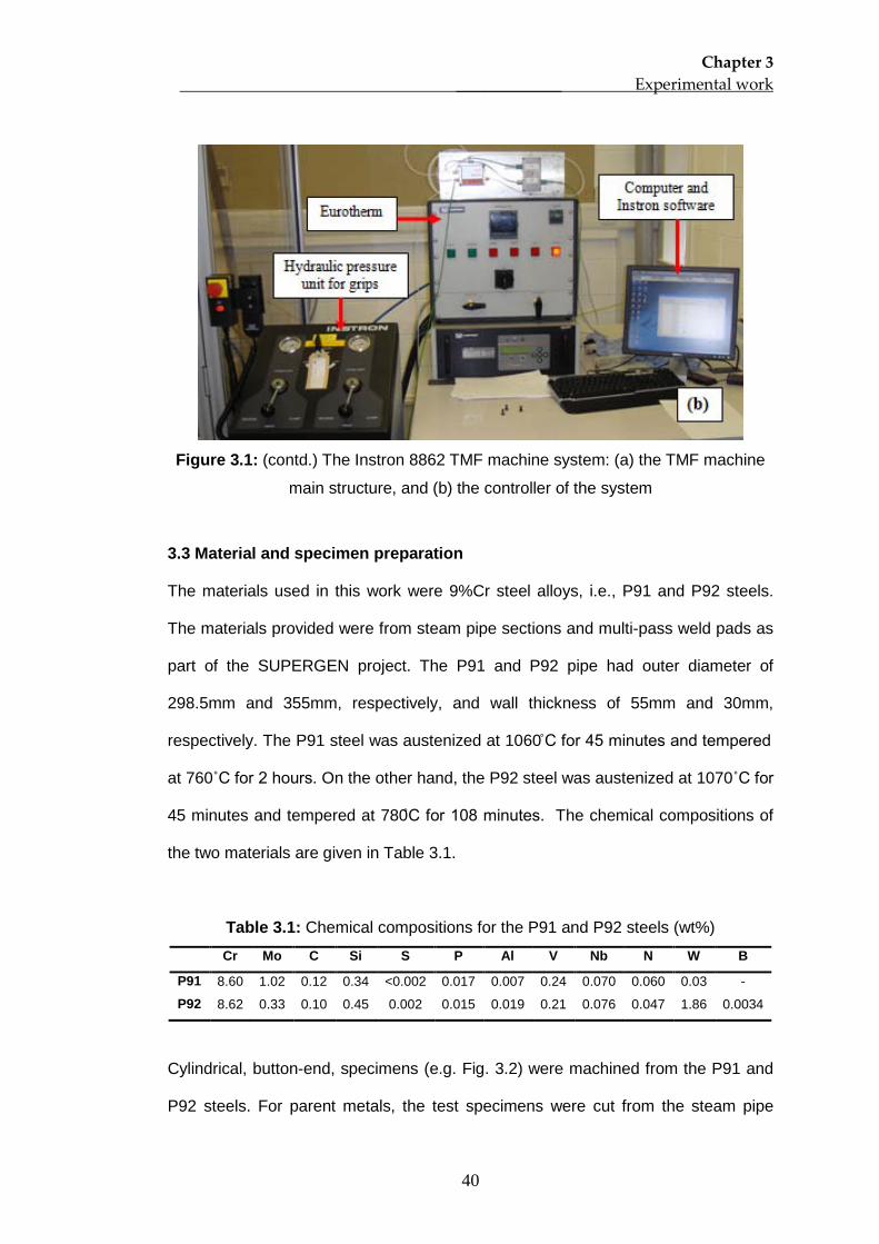
Figure 3.1: The Instron 8862 TMF machine system: (a) the TMF machine main
structure, and (b) the controller of the system
Chapter 3 _____________ Experimental work
40
Figure 3.1: (contd.) The Instron 8862 TMF machine system: (a) the TMF machine
main structure, and (b) the controller of the system
3.3 Material and specimen preparation
The materials used in this work were 9%Cr steel alloys, i.e., P91 and P92 steels.
The materials provided were from steam pipe sections and multi-pass weld pads as
part of the SUPERGEN project. The P91 and P92 pipe had outer diameter of
298.5mm and 355mm, respectively, and wall thickness of 55mm and 30mm,
respectively. The P91 steel was austenized at 1060̊ C for 45 minutes and tempered
at 760˚C for 2 hours. On the other hand, the P92 steel was austenized at 1070˚C for
45 minutes and tempered at 780̊C for 108 minutes. The chemical compositions of
the two materials are given in Table 3.1.
Table 3.1: Chemical compositions for the P91 and P92 steels (wt%)
Cr Mo C Si S P Al V Nb N W B
P91 8.60 1.02 0.12 0.34 <0.002 0.017 0.007 0.24 0.070 0.060 0.03 -
P92 8.62 0.33 0.10 0.45 0.002 0.015 0.019 0.21 0.076 0.047 1.86 0.0034
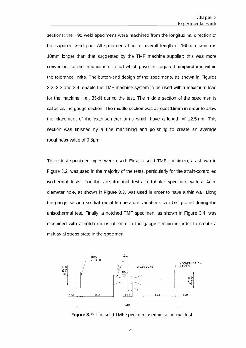
Cylindrical, button-end, specimens (e.g. Fig. 3.2) were machined from the P91 and
P92 steels. For parent metals, the test specimens were cut from the steam pipe
Chapter 3 _____________ Experimental work
41
sections; the P92 weld specimens were machined from the longitudinal direction of
the supplied weld pad. All specimens had an overall length of 160mm, which is
10mm longer than that suggested by the TMF machine supplier; this was more
convenient for the production of a coil which gave the required temperatures within
the tolerance limits. The button-end design of the specimens, as shown in Figures
3.2, 3.3 and 3.4, enable the TMF machine system to be used within maximum load
for the machine, i.e., 35kN during the test. The middle section of the specimen is
called as the gauge section. The middle section was at least 15mm in order to allow
the placement of the extensometer arms which have a length of 12.5mm. This
section was finished by a fine machining and polishing to create an average
roughness value of 0.8μm.
Three test specimen types were used. First, a solid TMF specimen, as shown in
Figure 3.2, was used in the majority of the tests, particularly for the strain-controlled
isothermal tests. For the anisothermal tests, a tubular specimen with a 4mm
diameter hole, as shown in Figure 3.3, was used in order to have a thin wall along
the gauge section so that radial temperature variations can be ignored during the
anisothermal test. Finally, a notched TMF specimen, as shown in Figure 3.4, was
machined with a notch radius of 2mm in the gauge section in order to create a
multiaxial stress state in the specimen.
Figure 3.2: The solid TMF specimen used in isothermal test
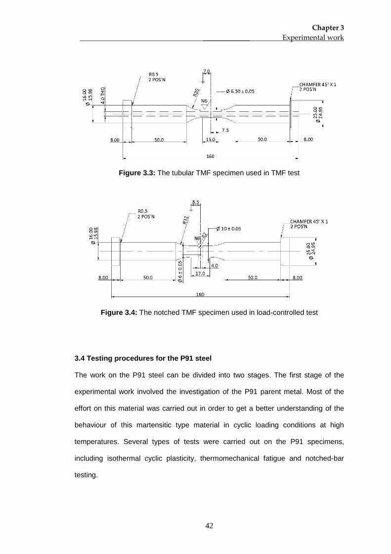
Chapter 3 _____________ Experimental work
42
Figure 3.3: The tubular TMF specimen used in TMF test
Figure 3.4: The notched TMF specimen used in load-controlled test
3.4 Testing procedures for the P91 steel
The work on the P91 steel can be divided into two stages. The first stage of the
experimental work involved the investigation of the P91 parent metal. Most of the
effort on this material was carried out in order to get a better understanding of the
behaviour of this martensitic type material in cyclic loading conditions at high
temperatures. Several types of tests were carried out on the P91 specimens,
including isothermal cyclic plasticity, thermomechanical fatigue and notched-bar
testing.
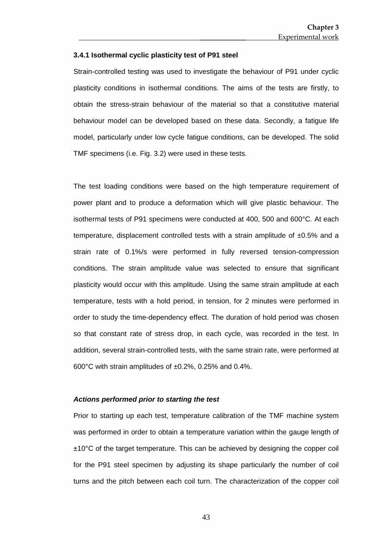
Chapter 3 _____________ Experimental work
43
3.4.1 Isothermal cyclic plasticity test of P91 steel
Strain-controlled testing was used to investigate the behaviour of P91 under cyclic
plasticity conditions in isothermal conditions. The aims of the tests are firstly, to
obtain the stress-strain behaviour of the material so that a constitutive material
behaviour model can be developed based on these data. Secondly, a fatigue life
model, particularly under low cycle fatigue conditions, can be developed. The solid
TMF specimens (i.e. Fig. 3.2) were used in these tests.
The test loading conditions were based on the high temperature requirement of
power plant and to produce a deformation which will give plastic behaviour. The
isothermal tests of P91 specimens were conducted at 400, 500 and 600°C. At each
temperature, displacement controlled tests with a strain amplitude of ±0.5% and a
strain rate of 0.1%/s were performed in fully reversed tension-compression
conditions. The strain amplitude value was selected to ensure that significant
plasticity would occur with this amplitude. Using the same strain amplitude at each
temperature, tests with a hold period, in tension, for 2 minutes were performed in
order to study the time-dependency effect. The duration of hold period was chosen
so that constant rate of stress drop, in each cycle, was recorded in the test. In
addition, several strain-controlled tests, with the same strain rate, were performed at
600°C with strain amplitudes of ±0.2%, 0.25% and 0.4%.
Actions performed prior to starting the test
Prior to starting up each test, temperature calibration of the TMF machine system
was performed in order to obtain a temperature variation within the gauge length of
±10°C of the target temperature. This can be achieved by designing the copper coil
for the P91 steel specimen by adjusting its shape particularly the number of coil
turns and the pitch between each coil turn. The characterization of the copper coil
Chapter 3 _____________ Experimental work
44
shape controls the density of magnetic flux, induced by the induction heating
system, and thus determines the specimen’s temperature. Five thermocouples were
welded on the gauge section, as shown in Figure 3.5, to measure the temperature
during thermal calibration. A coil from previous tests on a RR1000 specimen, as
shown in Figure 3.6(a) which gave temperature gradient of within ±10°C for the
RR1000, was used as a starting design shape. However, that coil design produced
a temperature variation of more than ±15°C, even after adjusting the pitch of coil
turn. Another shape of coil as shown in Figure 3.6(b) was used and there was an
improvement for temperature reading. The final design of the coil shape for P91
specimen tests is shown in Figure 3.7; this gave the required temperature variation
along the gauge section as plotted in Figure 3.8.
For the P91 steel isothermal strain-controlled tests, the temperatures during the
tests were measured by using thermocouples (TC). Two K-type thermocouples
were used in each test; one thermocouple acted as the main TC which controls the
required temperature for a test and another thermocouple was used to check the
reading of the main TC before starting the test. The thermocouple wires were
attached to the specimen’s surface by spot welding and the distance between the
two thermocouple wires must be less than 1mm as suggested by Hahner et al.
(2008). If the TC readings indicate an unacceptable variation of temperature, the
qualities of the spot welds are checked and repetition of the spot welding process
may be performed if necessary.
From previous tests on RR1000, using the TMF machine system (Hyde, 2010),
cracks were found at the TC spot weld positions on the gauge section. In order to
avoid that situation, temperature in the strain-controlled tests of P91 steel was
measured by positioning thermocouples away from the gauge section, i.e., on the
Chapter 3 _____________ Experimental work
45
shoulder of the specimen. Thus, the temperature ratio between the centre of the
gauge section and the specimen’s shoulder were recorded, at the position shown in
Figure 3.9(a). Average temperature readings at the shoulder position for
corresponding gauge section temperatures of 400, 500 and 600°C, obtained from
the setup of this experiment, were 344, 429 and 516°C, respectively. For the actual
tests, both thermocouples were placed on the specimen’s shoulder, as shown in
Figure 3.9(b), and the temperature ratios were used in the test.
In order to obtain a good response for a specified test loading, the PID (proportional,
integral, derivative) values of the TMF machine system were tuned. The strain
amplitudes and testing periods for the actual tests were applied on a specimen and
the PID values were adjusted accordingly to get a good fit to controlled shape
parameter (strain, load or temperature). The values of P 36, I 2 and D 0 were used
for the P91 steel tests determined by trial-and-error process. This procedure was
performed using the temperature calibration specimen.
Actual test
Once the temperature calibration and PID tuning procedures were completed, the
actual tests were performed, using new P91 specimens. Thermocouples were
instrumented on the specimen as shown in Figure 3.9(b) and then, the specimen
was installed on the test rig, as shown in Figure 3.7. A verification of Young’s
modulus was performed at room temperature to ensure correct operation of the
extensometer. The applied load in the Young’s modulus verification was small, to
ensure that it was within the elastic limit, in order to avoid an irreversible
displacement in the specimen before starting the test. Correct operation of the
extensometer resulted in a reasonable smooth plot of linear data and the measured
Young’s modulus values were comparable to reference values at the same
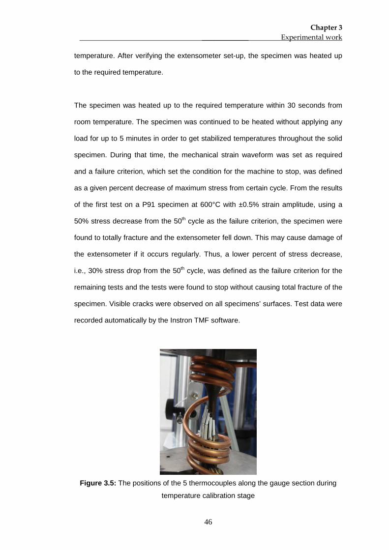
Chapter 3 _____________ Experimental work
46
temperature. After verifying the extensometer set-up, the specimen was heated up
to the required temperature.
The specimen was heated up to the required temperature within 30 seconds from
room temperature. The specimen was continued to be heated without applying any
load for up to 5 minutes in order to get stabilized temperatures throughout the solid
specimen. During that time, the mechanical strain waveform was set as required
and a failure criterion, which set the condition for the machine to stop, was defined
as a given percent decrease of maximum stress from certain cycle. From the results
of the first test on a P91 specimen at 600°C with ±0.5% strain amplitude, using a
50% stress decrease from the 50th cycle as the failure criterion, the specimen were
found to totally fracture and the extensometer fell down. This may cause damage of
the extensometer if it occurs regularly. Thus, a lower percent of stress decrease,
i.e., 30% stress drop from the 50th
cycle, was defined as the failure criterion for the
remaining tests and the tests were found to stop without causing total fracture of the
specimen. Visible cracks were observed on all specimens’ surfaces. Test data were
recorded automatically by the Instron TMF software.
Figure 3.5: The positions of the 5 thermocouples along the gauge section during
temperature calibration stage
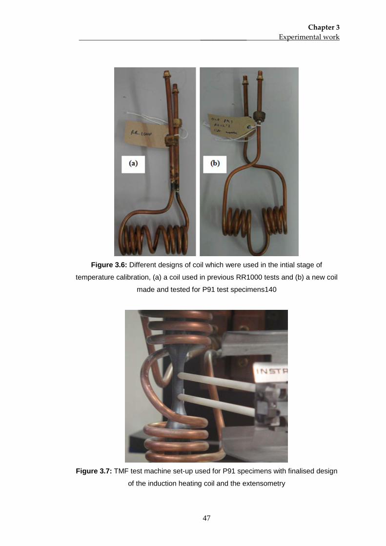
Chapter 3 _____________ Experimental work
47
Figure 3.6: Different designs of coil which were used in the intial stage of
temperature calibration, (a) a coil used in previous RR1000 tests and (b) a new coil
made and tested for P91 test specimens140
Figure 3.7: TMF test machine set-up used for P91 specimens with finalised design
of the induction heating coil and the extensometry
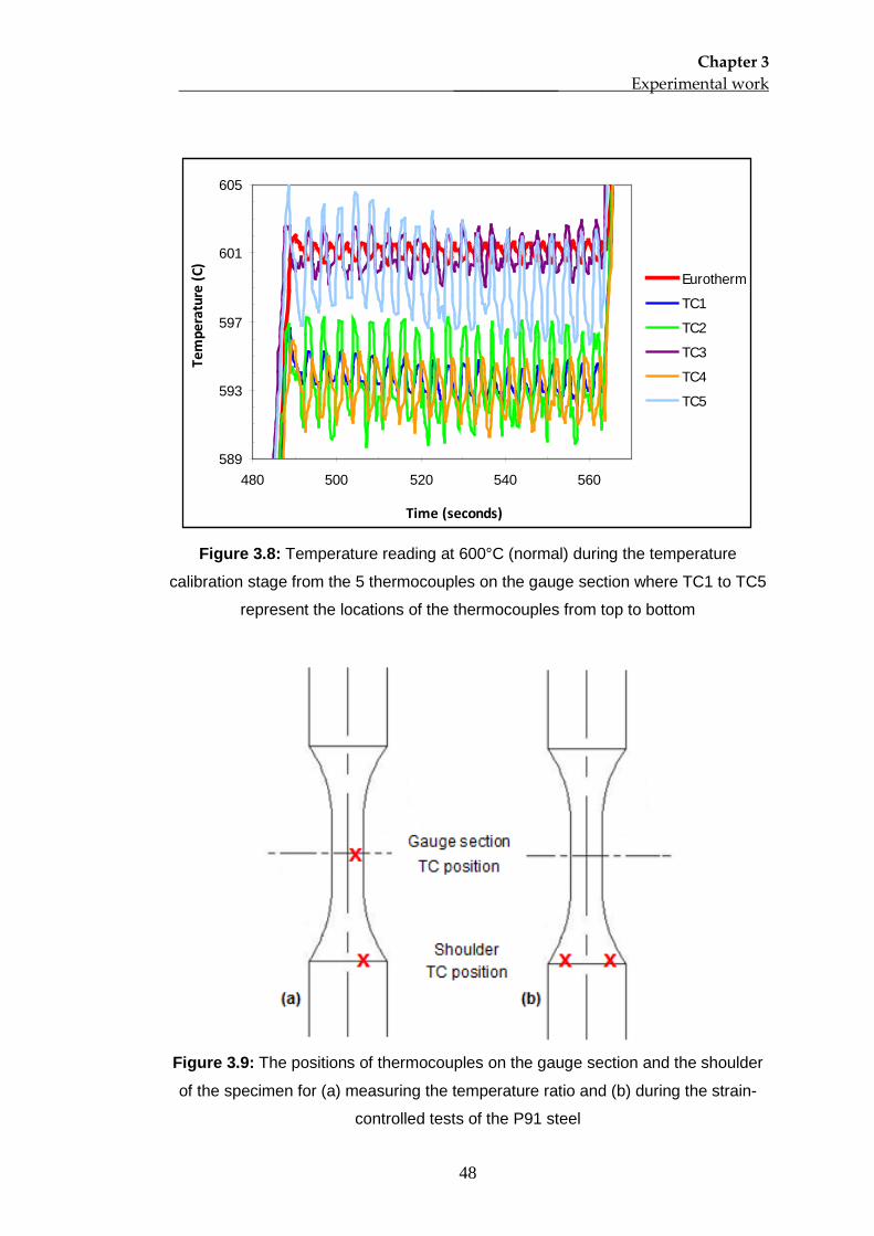
Chapter 3 _____________ Experimental work
48
589
593
597
601
605
480 500 520 540 560
Time (seconds)
Tem
pera
ture
(C)
Eurotherm
TC1
TC2
TC3
TC4
TC5
Figure 3.8: Temperature reading at 600°C (normal) during the temperature
calibration stage from the 5 thermocouples on the gauge section where TC1 to TC5
represent the locations of the thermocouples from top to bottom
Figure 3.9: The positions of thermocouples on the gauge section and the shoulder
of the specimen for (a) measuring the temperature ratio and (b) during the strain-
controlled tests of the P91 steel
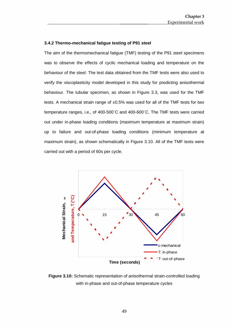
Chapter 3 _____________ Experimental work
49
3.4.2 Thermo-mechanical fatigue testing of P91 steel
The aim of the thermomechanical fatigue (TMF) testing of the P91 steel specimens
was to observe the effects of cyclic mechanical loading and temperature on the
behaviour of the steel. The test data obtained from the TMF tests were also used to
verify the viscoplasticity model developed in this study for predicting anisothermal
behaviour. The tubular specimen, as shown in Figure 3.3, was used for the TMF
tests. A mechanical strain range of ±0.5% was used for all of the TMF tests for two
temperature ranges, i.e., of 400-500˚C and 400-600˚C. The TMF tests were carried
out under in-phase loading conditions (maximum temperature at maximum strain)
up to failure and out-of-phase loading conditions (minimum temperature at
maximum strain), as shown schematically in Figure 3.10. All of the TMF tests were
carried out with a period of 60s per cycle.
0 15 30 45 60
Time (seconds)
Mec
hani
cal S
trai
n,
m
ɛ-mechanical
T: in-phase
T: out-of-phase
and
Tem
pera
ture
, T (°
C)
Figure 3.10: Schematic representation of anisothermal strain-controlled loading
with in-phase and out-of-phase temperature cycles
Chapter 3 _____________ Experimental work
50
An infra-red pyrometer was used instead of thermocouples at the specimen
shoulders to measure temperatures in the TMF tests. The controlled temperature at
the specimen’s shoulder causes difficulty in determining the temperature along the
gauge section when temperature is cycled. A pyrometer is a non-contacting device
for measuring the temperature and hence surface crack due to spot-welding can be
avoided. However, an oxide layer, which forms during testing, may affect the
accuracy of temperature measurement (Beck and Rau, 2008). An initial study was
implemented to assess the severity of the oxide layer formed during the test by
preoxidising the specimen at 650°C for 24 hours. It was found that the P91
specimen surface was not significantly oxidised compared to other specimens used
in previous tests in the lab such as stainless steel and RR1000 specimens. Thus,
the effect of oxidation on pyrometer reading was neglected in this study.
In order to use the pyrometer in the test, the emissivity values for the required
temperature between 400 and 600°C were determined prior to starting the TMF test.
For this purpose, the initial thermal cycling study was performed by attaching 5
thermocouples on the gauge section’s surface to measure the temperature
variation, as shown in Figure 3.5. The temperatures of the specimens in the tests
were controlled by the use of the middle thermocouple. The specimen was heated
to a specified temperature and the temperature was kept constant for several
minutes to stabilize the temperature of the specimen. The corresponding emissivity
value was then recorded. This process was repeated at other temperatures within
the required temperature range. The recorded emissivity values at 400, 500 and
600°C are 0.615, 0.625 and 0.635 respectively. Each emissivity value was then
used in a temperature cycling test, controlled by pyrometer. This was done in order
to get an emissivity value which can give a better temperature reading for the
specified temperature range and to ensure that the maximum temperature
Chapter 3 _____________ Experimental work
51
variations within gauge length of the specimen are within the required range, i.e.,
±10°C (Hahner et al., 2008). The emissivity value of 0.625 was used in the TMF
tests.
For the thermomechanical fatigue test, the TMF software divides the test into four
stages, namely, stabilisation, measurement, verification and test stage. The first
three stages were the preparatory stages in which only a temperature waveform
was applied and resultant thermal strains were measured and verified. The thermal
strain was measured by using the extensometers data and recorded at the base
time interval. In the test stage, the mechanical strain cycle of ±0.5% was defined in
the TMF software; the mechanical strain can only be realized by controlling the total
strain applied to the specimen considering the thermal strain measured in the
preparatory stages. For example, the total strain applied to a specimen in the
tension direction, for TMF in-phase tests was higher than the defined mechanical
strain due to the contribution of thermal strain (expansion of specimen due to
increase of temperature). In contrast, the thermal and mechanical strains were
opposite in direction for the TMF out-of-phase tests and hence resulted in shorter
applied total strain in the test. The 30% stress drop from the 50th
cycle was also
used as the failure criterion for the TMF test.
3.4.2 Cyclic notched bar test of P91 steel
The cyclic notched bar tests on P91 steel were performed using a fully reversed
load-controlled condition in order to verify the capability of the material model under
multiaxial conditions. The nominal stress amplitude was 300MPa on the minimum
notch section and a constant temperature of 600°C was applied to the specimens
throughout the test. The stress value was chosen in order to produce a similar strain
range effect, on the notch section, as that in the isothermal strain-controlled tests on
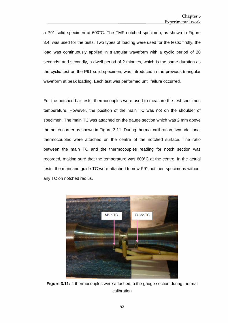
Chapter 3 _____________ Experimental work
52
a P91 solid specimen at 600°C. The TMF notched specimen, as shown in Figure
3.4, was used for the tests. Two types of loading were used for the tests: firstly, the
load was continuously applied in triangular waveform with a cyclic period of 20
seconds; and secondly, a dwell period of 2 minutes, which is the same duration as
the cyclic test on the P91 solid specimen, was introduced in the previous triangular
waveform at peak loading. Each test was performed until failure occurred.
For the notched bar tests, thermocouples were used to measure the test specimen
temperature. However, the position of the main TC was not on the shoulder of
specimen. The main TC was attached on the gauge section which was 2 mm above
the notch corner as shown in Figure 3.11. During thermal calibration, two additional
thermocouples were attached on the centre of the notched surface. The ratio
between the main TC and the thermocouples reading for notch section was
recorded, making sure that the temperature was 600°C at the centre. In the actual
tests, the main and guide TC were attached to new P91 notched specimens without
any TC on notched radius.
Figure 3.11: 4 thermocouples were attached to the gauge section during thermal
calibration
Chapter 3 _____________ Experimental work
53
3.5 Testing procedures for the P92 steel
The second stage of the experimental work was performed on P92 parent material
and weld metal. Isothermal strain controlled and thermomechanical fatigue tests
were carried out on P92 specimens using the same TMF machine system, in which
the solid and tubular TMF specimens designs already described, were used,
respectively. The difference was that the maximum test temperature was increased
to 675°C, to reflect the higher temperature capability of P92 compared with P91 in
real applications. The isothermal tests were performed at 500, 600 and 675°C with a
strain amplitude of ±0.5% and a strain rate of 0.1%/s. Then, tests with dwell periods
of 5 minutes at the peak tensile strain were also performed for each temperature.
The thermomechanical fatigue tests were carried out in a temperature range of 500
to 675°C with in-phase and out-of-phase loading, with a 60 seconds cycle period.
The isothermal and TMF tests, of the P92 parent and weld specimens, were
performed using the same procedures as have been described for the P91 parent
metal specimens, except for the temperature measurement method. For this stage,
the main thermocouples, which controlled the test temperature, were attached in the
middle of gauge section for both the isothermal and the TMF tests, as shown in
Figure 3.12(a). From trial tests on P91 specimen at the end of stage 1, it seems that
cracks may not have initiated at welding point of the thermocouple wires, as found
in the works of Hyde (2010) for RR1000 specimens, if care is taken during the spot
welding, i.e., the lowest possible current is used which will ensure that the contact
between thermocouple wires and specimen’s surface is strong enough. In addition,
a solid specimen was used in all of the strain-controlled tests for this study, rather
than the tubular specimens used in the strain-controlled tests for the previous study.
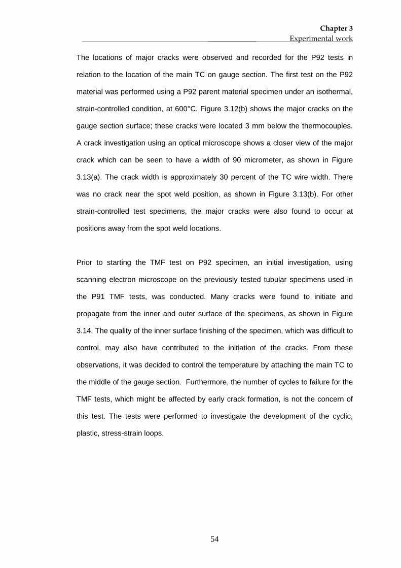
Chapter 3 _____________ Experimental work
54
The locations of major cracks were observed and recorded for the P92 tests in
relation to the location of the main TC on gauge section. The first test on the P92
material was performed using a P92 parent material specimen under an isothermal,
strain-controlled condition, at 600°C. Figure 3.12(b) shows the major cracks on the
gauge section surface; these cracks were located 3 mm below the thermocouples.
A crack investigation using an optical microscope shows a closer view of the major
crack which can be seen to have a width of 90 micrometer, as shown in Figure
3.13(a). The crack width is approximately 30 percent of the TC wire width. There
was no crack near the spot weld position, as shown in Figure 3.13(b). For other
strain-controlled test specimens, the major cracks were also found to occur at
positions away from the spot weld locations.
Prior to starting the TMF test on P92 specimen, an initial investigation, using
scanning electron microscope on the previously tested tubular specimens used in
the P91 TMF tests, was conducted. Many cracks were found to initiate and
propagate from the inner and outer surface of the specimens, as shown in Figure
3.14. The quality of the inner surface finishing of the specimen, which was difficult to
control, may also have contributed to the initiation of the cracks. From these
observations, it was decided to control the temperature by attaching the main TC to
the middle of the gauge section. Furthermore, the number of cycles to failure for the
TMF tests, which might be affected by early crack formation, is not the concern of
this test. The tests were performed to investigate the development of the cyclic,
plastic, stress-strain loops.
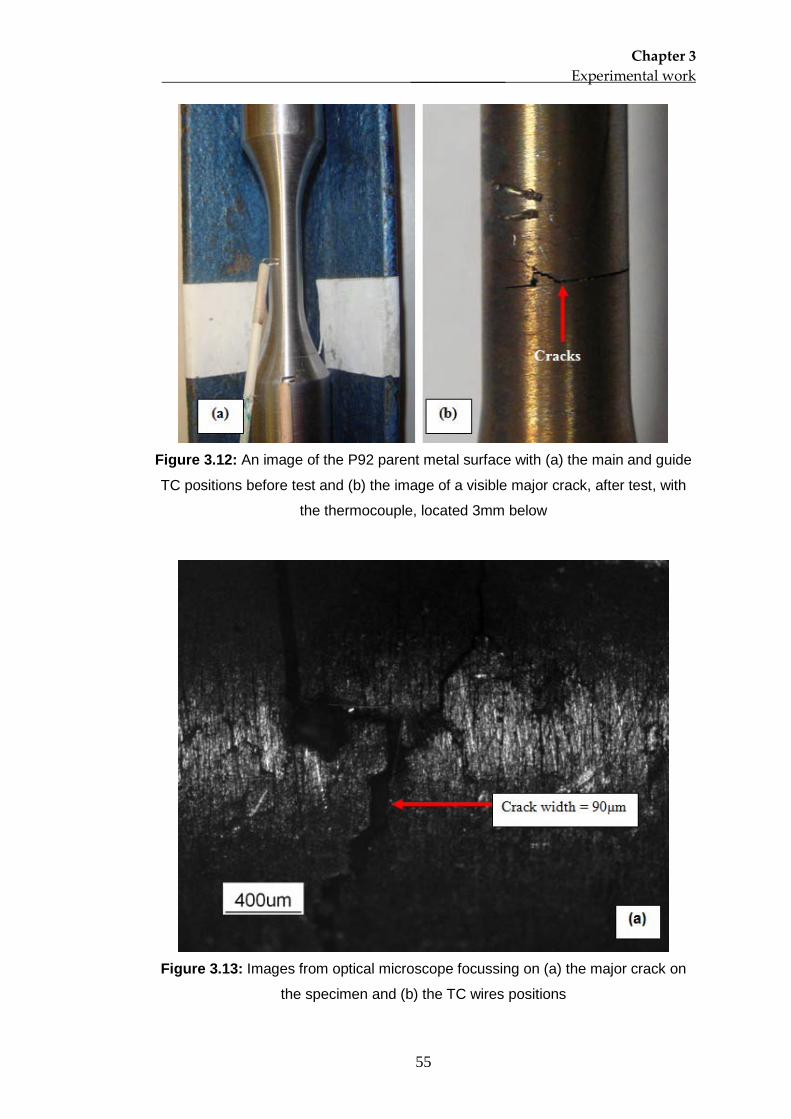
Chapter 3 _____________ Experimental work
55
Figure 3.12: An image of the P92 parent metal surface with (a) the main and guide
TC positions before test and (b) the image of a visible major crack, after test, with
the thermocouple, located 3mm below
Figure 3.13: Images from optical microscope focussing on (a) the major crack on
the specimen and (b) the TC wires positions
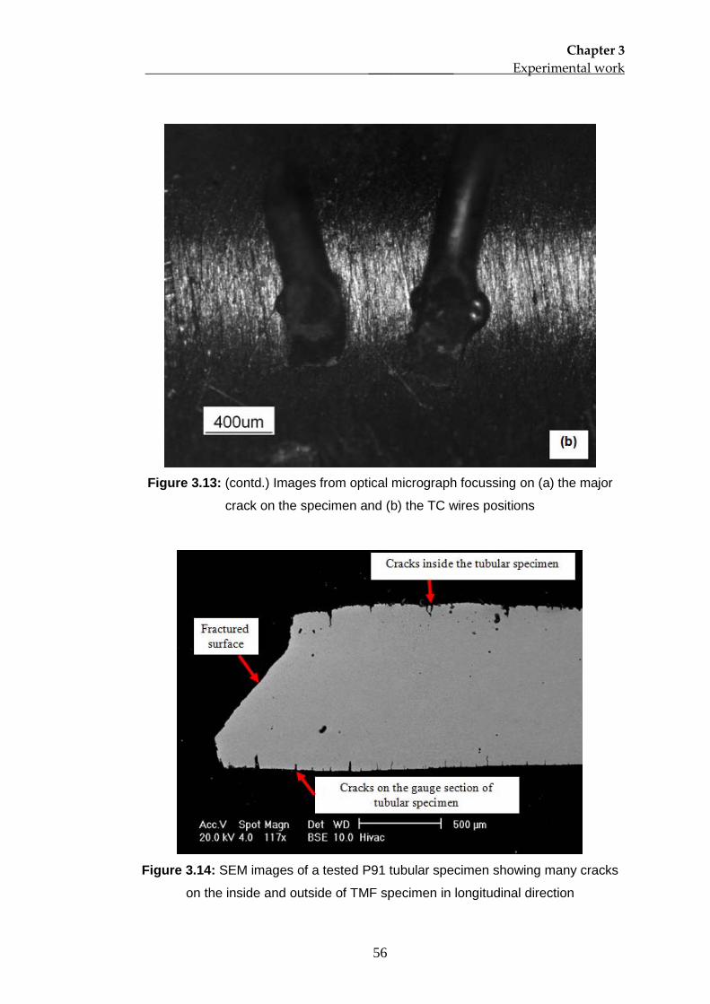
Chapter 3 _____________ Experimental work
56
Figure 3.13: (contd.) Images from optical micrograph focussing on (a) the major
crack on the specimen and (b) the TC wires positions
Figure 3.14: SEM images of a tested P91 tubular specimen showing many cracks
on the inside and outside of TMF specimen in longitudinal direction
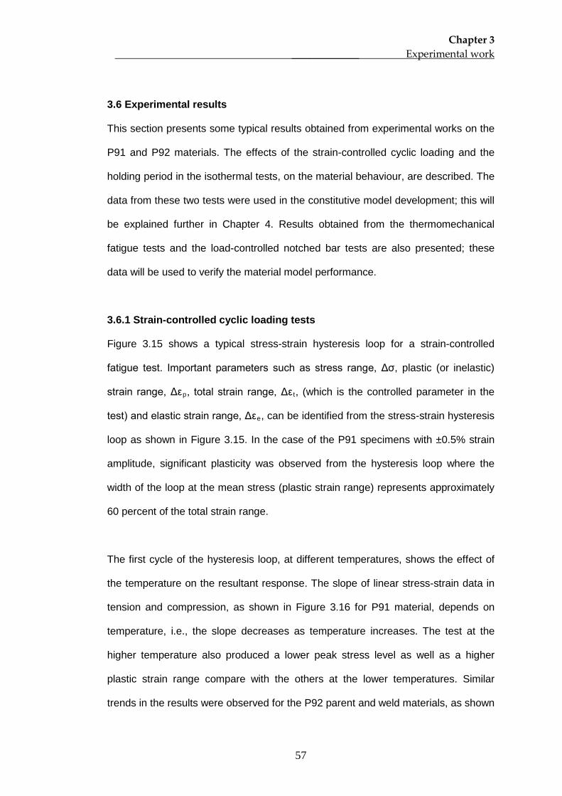
Chapter 3 _____________ Experimental work
57
3.6 Experimental results
This section presents some typical results obtained from experimental works on the
P91 and P92 materials. The effects of the strain-controlled cyclic loading and the
holding period in the isothermal tests, on the material behaviour, are described. The
data from these two tests were used in the constitutive model development; this will
be explained further in Chapter 4. Results obtained from the thermomechanical
fatigue tests and the load-controlled notched bar tests are also presented; these
data will be used to verify the material model performance.
3.6.1 Strain-controlled cyclic loading tests
Figure 3.15 shows a typical stress-strain hysteresis loop for a strain-controlled
fatigue test. Important parameters such as stress range, Δσ, plastic (or inelastic)
strain range, Δεp, total strain range, Δε t, (which is the controlled parameter in the
test) and elastic strain range, Δεe
, can be identified from the stress-strain hysteresis
loop as shown in Figure 3.15. In the case of the P91 specimens with ±0.5% strain
amplitude, significant plasticity was observed from the hysteresis loop where the
width of the loop at the mean stress (plastic strain range) represents approximately
60 percent of the total strain range.
The first cycle of the hysteresis loop, at different temperatures, shows the effect of
the temperature on the resultant response. The slope of linear stress-strain data in
tension and compression, as shown in Figure 3.16 for P91 material, depends on
temperature, i.e., the slope decreases as temperature increases. The test at the
higher temperature also produced a lower peak stress level as well as a higher
plastic strain range compare with the others at the lower temperatures. Similar
trends in the results were observed for the P92 parent and weld materials, as shown
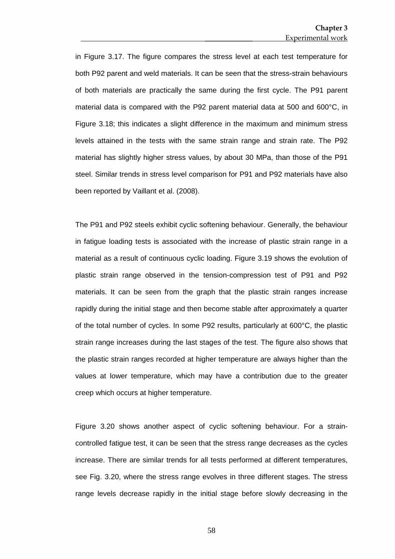
Chapter 3 _____________ Experimental work
58
in Figure 3.17. The figure compares the stress level at each test temperature for
both P92 parent and weld materials. It can be seen that the stress-strain behaviours
of both materials are practically the same during the first cycle. The P91 parent
material data is compared with the P92 parent material data at 500 and 600°C, in
Figure 3.18; this indicates a slight difference in the maximum and minimum stress
levels attained in the tests with the same strain range and strain rate. The P92
material has slightly higher stress values, by about 30 MPa, than those of the P91
steel. Similar trends in stress level comparison for P91 and P92 materials have also
been reported by Vaillant et al. (2008).
The P91 and P92 steels exhibit cyclic softening behaviour. Generally, the behaviour
in fatigue loading tests is associated with the increase of plastic strain range in a
material as a result of continuous cyclic loading. Figure 3.19 shows the evolution of
plastic strain range observed in the tension-compression test of P91 and P92
materials. It can be seen from the graph that the plastic strain ranges increase
rapidly during the initial stage and then become stable after approximately a quarter
of the total number of cycles. In some P92 results, particularly at 600°C, the plastic
strain range increases during the last stages of the test. The figure also shows that
the plastic strain ranges recorded at higher temperature are always higher than the
values at lower temperature, which may have a contribution due to the greater
creep which occurs at higher temperature.
Figure 3.20 shows another aspect of cyclic softening behaviour. For a strain-
controlled fatigue test, it can be seen that the stress range decreases as the cycles
increase. There are similar trends for all tests performed at different temperatures,
see Fig. 3.20, where the stress range evolves in three different stages. The stress
range levels decrease rapidly in the initial stage before slowly decreasing in the
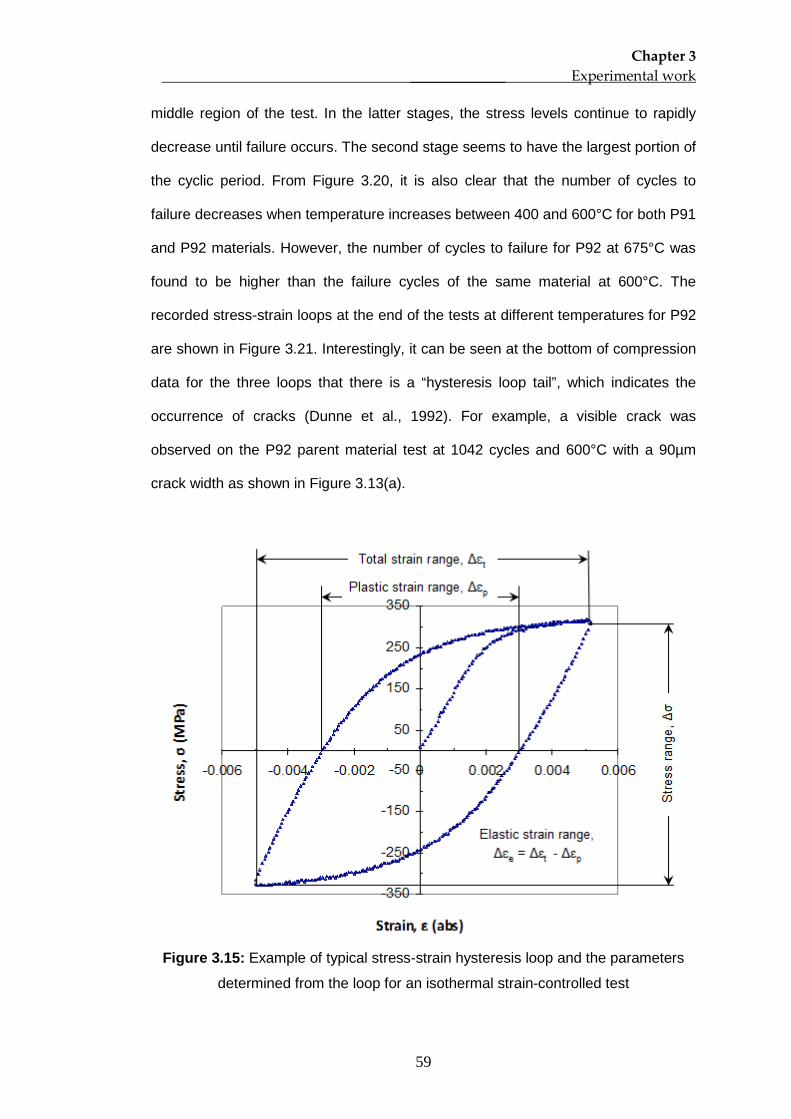
Chapter 3 _____________ Experimental work
59
middle region of the test. In the latter stages, the stress levels continue to rapidly
decrease until failure occurs. The second stage seems to have the largest portion of
the cyclic period. From Figure 3.20, it is also clear that the number of cycles to
failure decreases when temperature increases between 400 and 600°C for both P91
and P92 materials. However, the number of cycles to failure for P92 at 675°C was
found to be higher than the failure cycles of the same material at 600°C. The
recorded stress-strain loops at the end of the tests at different temperatures for P92
are shown in Figure 3.21. Interestingly, it can be seen at the bottom of compression
data for the three loops that there is a “hysteresis loop tail”, which indicates the
occurrence of cracks (Dunne et al., 1992). For example, a visible crack was
observed on the P92 parent material test at 1042 cycles and 600°C with a 90µm
crack width as shown in Figure 3.13(a).
Figure 3.15: Example of typical stress-strain hysteresis loop and the parameters
determined from the loop for an isothermal strain-controlled test
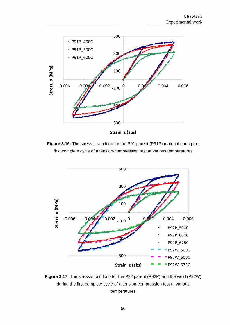
Chapter 3 _____________ Experimental work
60
-500
-300
-100
100
300
500
-0.006 -0.004 -0.002 0 0.002 0.004 0.006
Strain, ε (abs)
Str
ess,
σ (M
Pa)
P91P_400C
P91P_500C
P91P_600C
Figure 3.16: The stress-strain loop for the P91 parent (P91P) material during the
first complete cycle of a tension-compression test at various temperatures
-500
-300
-100
100
300
500
-0.006 -0.004 -0.002 0 0.002 0.004 0.006
Strain, ε (abs)
Str
ess,
σ (M
Pa)
P92P_500C
P92P_600C
P92P_675C
P92W_500C
P92W_600C
P92W_675C
Figure 3.17: The stress-strain loop for the P92 parent (P92P) and the weld (P92W)
during the first complete cycle of a tension-compression test at various
temperatures
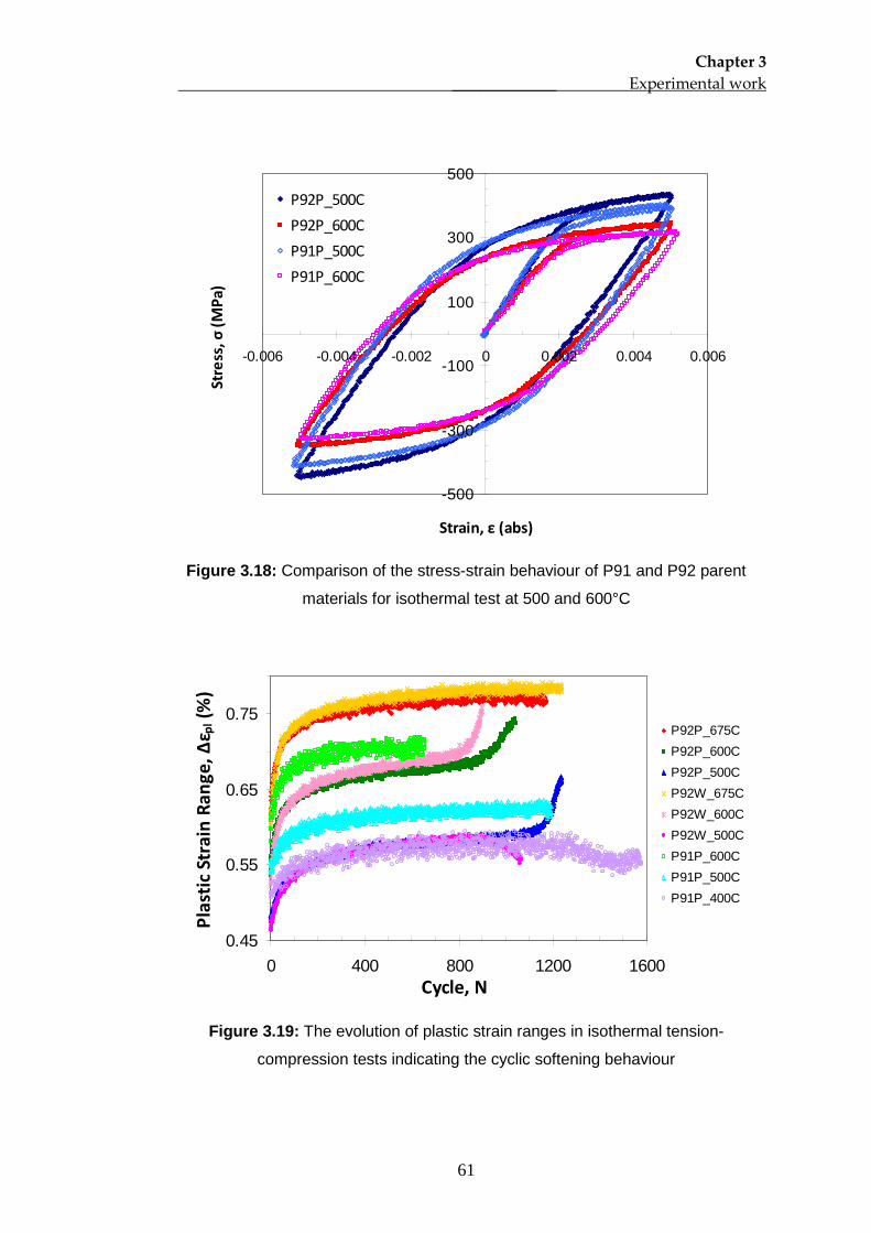
Chapter 3 _____________ Experimental work
61
-500
-300
-100
100
300
500
-0.006 -0.004 -0.002 0 0.002 0.004 0.006
Strain, ε (abs)
Str
ess,
σ (M
Pa)
P92P_500CP92P_600CP91P_500CP91P_600C
Figure 3.18: Comparison of the stress-strain behaviour of P91 and P92 parent
materials for isothermal test at 500 and 600°C
0.45
0.55
0.65
0.75
0 400 800 1200 1600Cycle, N
Plas
tic S
trai
n Ra
nge,
Δε p
l (%
)
P92P_675CP92P_600CP92P_500CP92W_675CP92W_600CP92W_500CP91P_600CP91P_500CP91P_400C
Figure 3.19: The evolution of plastic strain ranges in isothermal tension-
compression tests indicating the cyclic softening behaviour
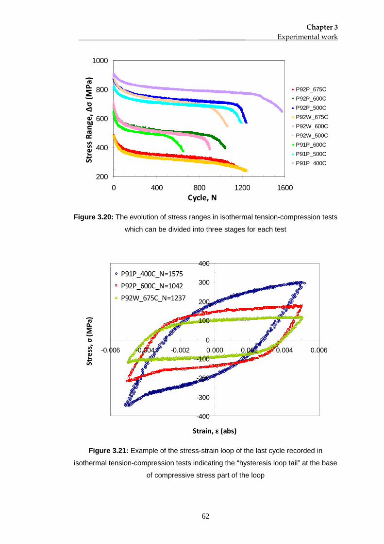
Chapter 3 _____________ Experimental work
62
200
400
600
800
1000
0 400 800 1200 1600Cycle, N
Stre
ss R
ange
, Δσ
(MPa
)P92P_675CP92P_600CP92P_500CP92W_675CP92W_600CP92W_500CP91P_600CP91P_500CP91P_400C
Figure 3.20: The evolution of stress ranges in isothermal tension-compression tests
which can be divided into three stages for each test
-400
-300
-200
-100
0
100
200
300
400
-0.006 -0.004 -0.002 0.000 0.002 0.004 0.006
Strain, ε (abs)
Str
ess,
σ (M
Pa)
P91P_400C_N=1575P92P_600C_N=1042P92W_675C_N=1237
Figure 3.21: Example of the stress-strain loop of the last cycle recorded in
isothermal tension-compression tests indicating the “hysteresis loop tail” at the base
of compressive stress part of the loop
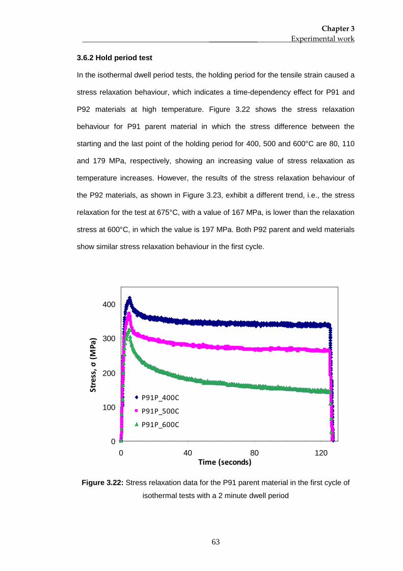
Chapter 3 _____________ Experimental work
63
3.6.2 Hold period test
In the isothermal dwell period tests, the holding period for the tensile strain caused a
stress relaxation behaviour, which indicates a time-dependency effect for P91 and
P92 materials at high temperature. Figure 3.22 shows the stress relaxation
behaviour for P91 parent material in which the stress difference between the
starting and the last point of the holding period for 400, 500 and 600°C are 80, 110
and 179 MPa, respectively, showing an increasing value of stress relaxation as
temperature increases. However, the results of the stress relaxation behaviour of
the P92 materials, as shown in Figure 3.23, exhibit a different trend, i.e., the stress
relaxation for the test at 675°C, with a value of 167 MPa, is lower than the relaxation
stress at 600°C, in which the value is 197 MPa. Both P92 parent and weld materials
show similar stress relaxation behaviour in the first cycle.
0
100
200
300
400
0 40 80 120Time (seconds)
Str
ess,
σ (M
Pa)
P91P_400C
P91P_500C
P91P_600C
Figure 3.22: Stress relaxation data for the P91 parent material in the first cycle of
isothermal tests with a 2 minute dwell period
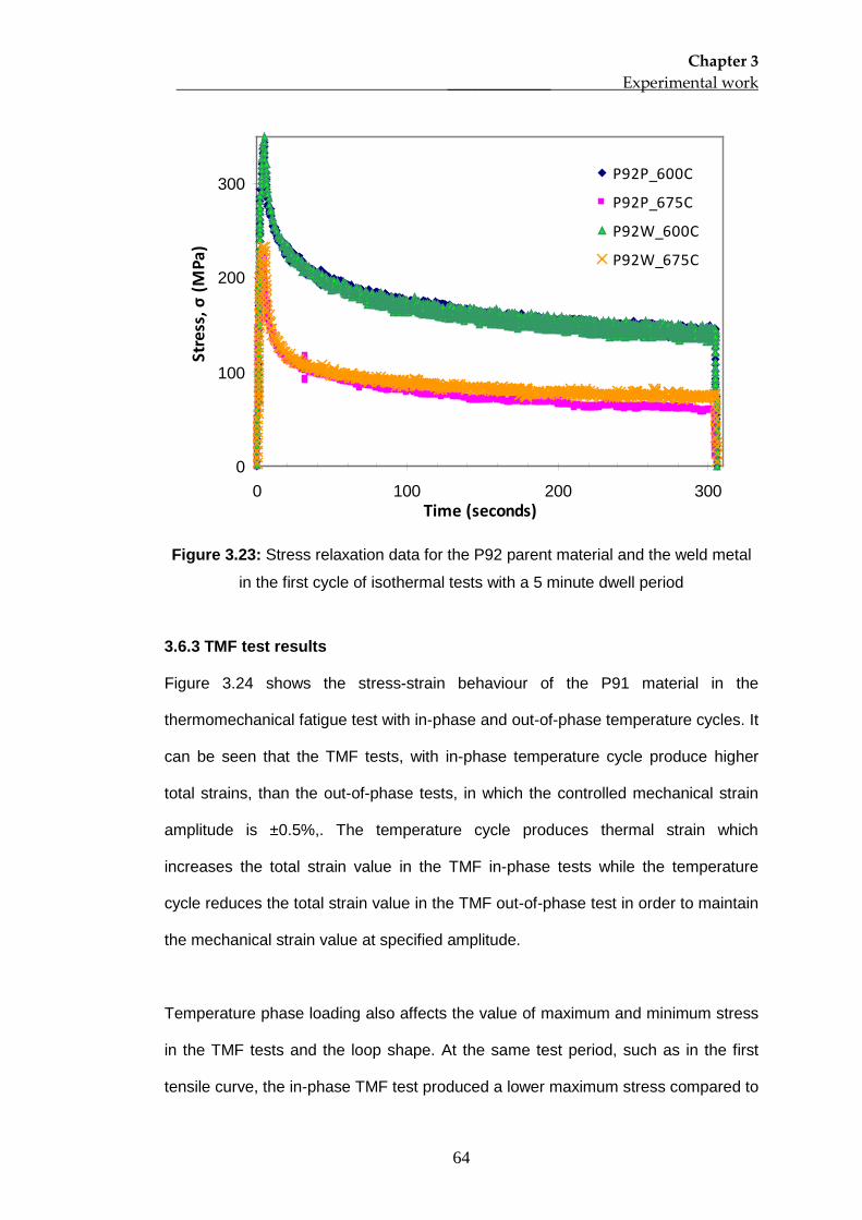
Chapter 3 _____________ Experimental work
64
0
100
200
300
0 100 200 300Time (seconds)
Str
ess,
σ (M
Pa)
P92P_600C
P92P_675C
P92W_600C
P92W_675C
Figure 3.23: Stress relaxation data for the P92 parent material and the weld metal
in the first cycle of isothermal tests with a 5 minute dwell period
3.6.3 TMF test results
Figure 3.24 shows the stress-strain behaviour of the P91 material in the
thermomechanical fatigue test with in-phase and out-of-phase temperature cycles. It
can be seen that the TMF tests, with in-phase temperature cycle produce higher
total strains, than the out-of-phase tests, in which the controlled mechanical strain
amplitude is ±0.5%,. The temperature cycle produces thermal strain which
increases the total strain value in the TMF in-phase tests while the temperature
cycle reduces the total strain value in the TMF out-of-phase test in order to maintain
the mechanical strain value at specified amplitude.
Temperature phase loading also affects the value of maximum and minimum stress
in the TMF tests and the loop shape. At the same test period, such as in the first
tensile curve, the in-phase TMF test produced a lower maximum stress compared to
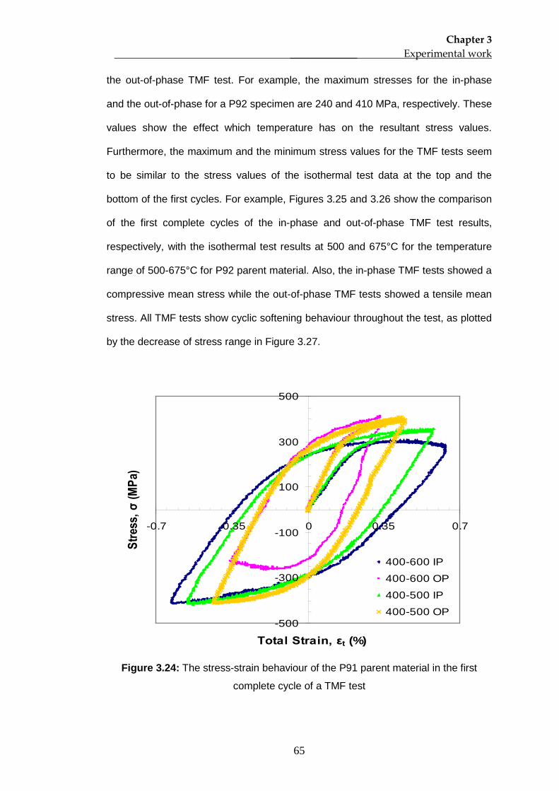
Chapter 3 _____________ Experimental work
65
the out-of-phase TMF test. For example, the maximum stresses for the in-phase
and the out-of-phase for a P92 specimen are 240 and 410 MPa, respectively. These
values show the effect which temperature has on the resultant stress values.
Furthermore, the maximum and the minimum stress values for the TMF tests seem
to be similar to the stress values of the isothermal test data at the top and the
bottom of the first cycles. For example, Figures 3.25 and 3.26 show the comparison
of the first complete cycles of the in-phase and out-of-phase TMF test results,
respectively, with the isothermal test results at 500 and 675°C for the temperature
range of 500-675°C for P92 parent material. Also, the in-phase TMF tests showed a
compressive mean stress while the out-of-phase TMF tests showed a tensile mean
stress. All TMF tests show cyclic softening behaviour throughout the test, as plotted
by the decrease of stress range in Figure 3.27.
-500
-300
-100
100
300
500
-0.7 -0.35 0 0.35 0.7
Total Strain, εt (%)
Stre
ss, σ
(MPa
)
400-600 IP
400-600 OP
400-500 IP
400-500 OP
Figure 3.24: The stress-strain behaviour of the P91 parent material in the first
complete cycle of a TMF test
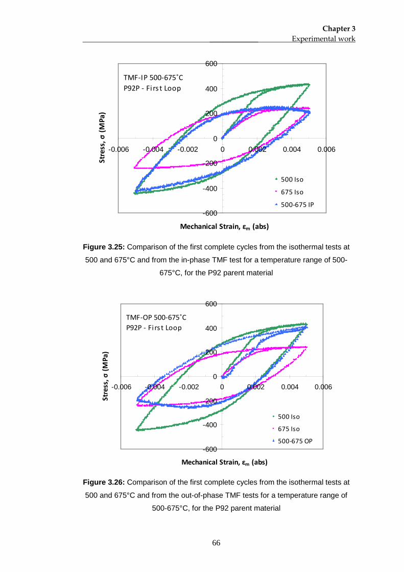
Chapter 3 _____________ Experimental work
66
-600
-400
-200
0
200
400
600
-0.006 -0.004 -0.002 0 0.002 0.004 0.006
Mechanical Strain, εm (abs)
Stre
ss, σ
(MPa
)
500 Iso
675 Iso
500-675 IP
TMF-IP 500-675˚CP92P - Fi rs t Loop
Figure 3.25: Comparison of the first complete cycles from the isothermal tests at
500 and 675°C and from the in-phase TMF test for a temperature range of 500-
675°C, for the P92 parent material
-600
-400
-200
0
200
400
600
-0.006 -0.004 -0.002 0 0.002 0.004 0.006
Mechanical Strain, εm (abs)
Stre
ss, σ
(MPa
)
500 Iso
675 Iso
500-675 OP
TMF-OP 500-675˚CP92P - Fi rs t Loop
Figure 3.26: Comparison of the first complete cycles from the isothermal tests at
500 and 675°C and from the out-of-phase TMF tests for a temperature range of
500-675°C, for the P92 parent material
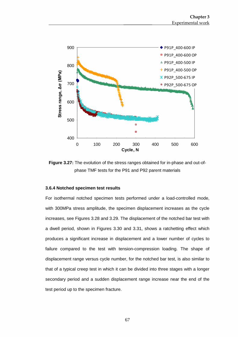
Chapter 3 _____________ Experimental work
67
400
500
600
700
800
900
0 100 200 300 400 500 600Cycle, N
Stre
ss ra
nge,
Δσ
(MPa
)
P91P_400-600 IP
P91P_400-600 OP
P91P_400-500 IP
P91P_400-500 OP
P92P_500-675 IP
P92P_500-675 OP
Figure 3.27: The evolution of the stress ranges obtained for in-phase and out-of-
phase TMF tests for the P91 and P92 parent materials
3.6.4 Notched specimen test results
For isothermal notched specimen tests performed under a load-controlled mode,
with 300MPa stress amplitude, the specimen displacement increases as the cycle
increases, see Figures 3.28 and 3.29. The displacement of the notched bar test with
a dwell period, shown in Figures 3.30 and 3.31, shows a ratchetting effect which
produces a significant increase in displacement and a lower number of cycles to
failure compared to the test with tension-compression loading. The shape of
displacement range versus cycle number, for the notched bar test, is also similar to
that of a typical creep test in which it can be divided into three stages with a longer
secondary period and a sudden displacement range increase near the end of the
test period up to the specimen fracture.
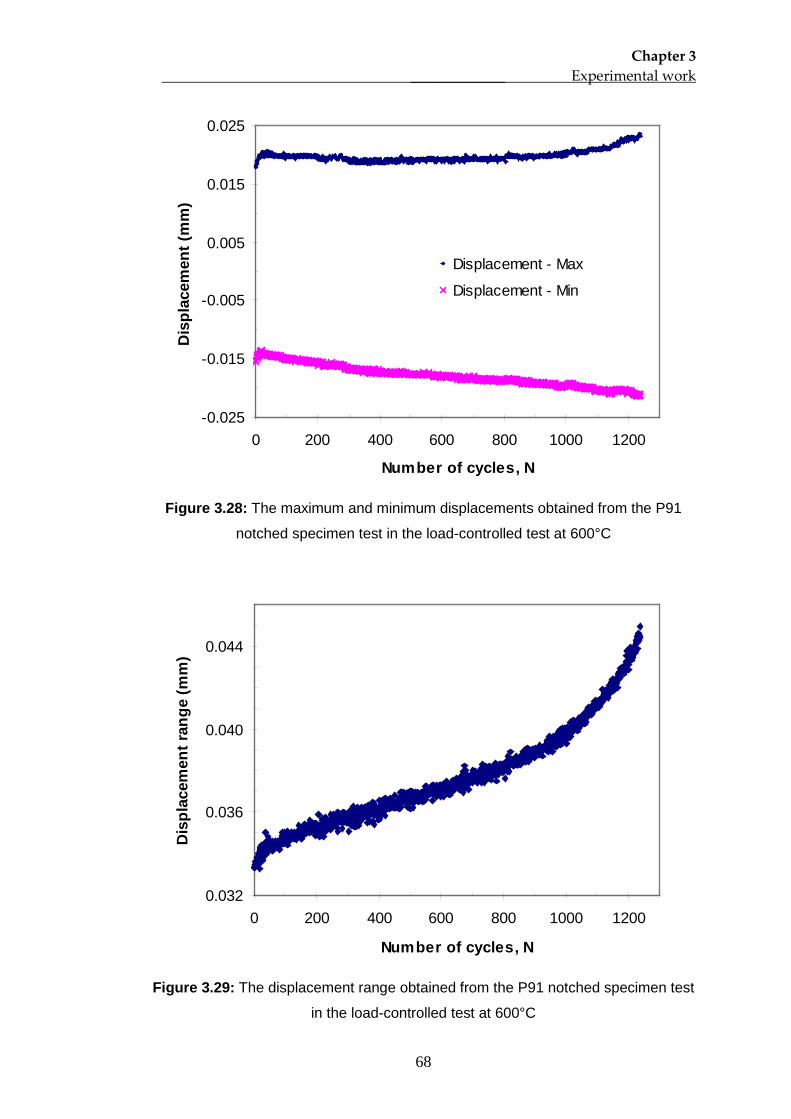
Chapter 3 _____________ Experimental work
68
-0.025
-0.015
-0.005
0.005
0.015
0.025
0 200 400 600 800 1000 1200
Number of cycles, N
Dis
plac
emen
t (m
m)
Displacement - Max
Displacement - Min
Figure 3.28: The maximum and minimum displacements obtained from the P91
notched specimen test in the load-controlled test at 600°C
0.032
0.036
0.040
0.044
0 200 400 600 800 1000 1200
Number of cycles, N
Dis
plac
emen
t ran
ge (m
m)
Figure 3.29: The displacement range obtained from the P91 notched specimen test
in the load-controlled test at 600°C
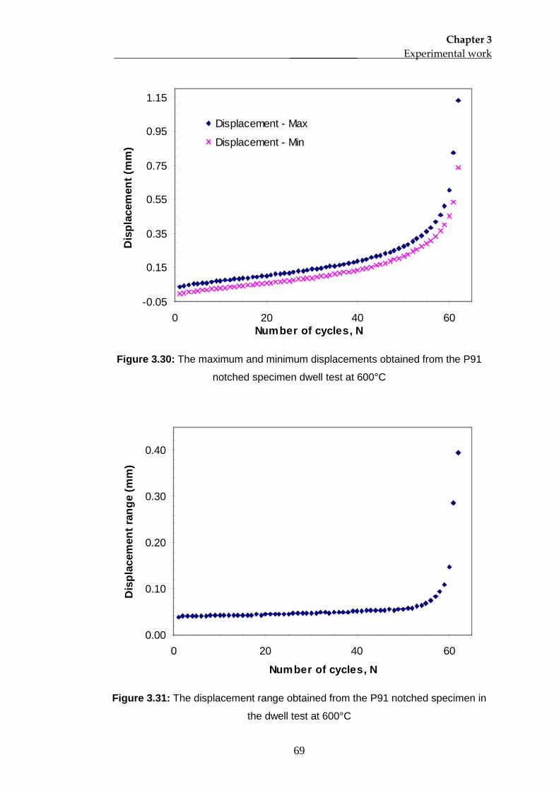
Chapter 3 _____________ Experimental work
69
-0.05
0.15
0.35
0.55
0.75
0.95
1.15
0 20 40 60Number of cycles, N
Dis
plac
emen
t (m
m)
Displacement - Max
Displacement - Min
Figure 3.30: The maximum and minimum displacements obtained from the P91
notched specimen dwell test at 600°C
0.00
0.10
0.20
0.30
0.40
0 20 40 60
Number of cycles, N
Dis
plac
emen
t ran
ge (m
m)
Figure 3.31: The displacement range obtained from the P91 notched specimen in
the dwell test at 600°C
Chapter 4 ________ Stress-strain analysis and microstructure investigation of cyclic tests
70
Chapter 4 –Stress-strain analysis and microstructure
investigation of cyclic tests
4.1 Overview
This chapter contains an analysis of the stress-strain behaviour, and its related
parameters, produced in strain-controlled tests of P91 steel, at 600°C. It also
contains an investigation of the microstructural variations which occur in specimens
during the cyclic tests. Based on the experimental stress-strain data, variations in
the Young’s modulus and the area enclosed in the hysteresis loops are determined,
together with the variations in other parameters throughout the test. The strain and
energy parameters obtained from strain-controlled tests with different strain
amplitudes can be used to develop fatigue lifing methods. Also, the results of the
microstructural investigations of the P91 steel, at different life fractions, using
scanning and transmission electron microscopes, are presented. Finally, the
relationships between the cyclic stress-strain data and the results obtained from the
microstructural investigations are used to gain an understanding of the cyclic
softening and failure mechanisms for the P91 steel.
4.2 Stress-strain analysis
Based on the results provided in Chapter 3, the P91 steel exhibited cyclic softening
behaviour in all of the tests performed in this study. From the isothermal, strain-
controlled tests, at 600̊ C , with different strain amplitudes, it can be seen that the
material exhibits cyclic softening behaviour as can be seen in Figures 4.1 and 4.2,
which present the evolutions of the maximum stress when various plastic strain
ranges are applied throughout the tests. The same strain rate of 0.1%/s was used
for all of the tests. Parameters such as Young’s modulus, hysteresis loop area and
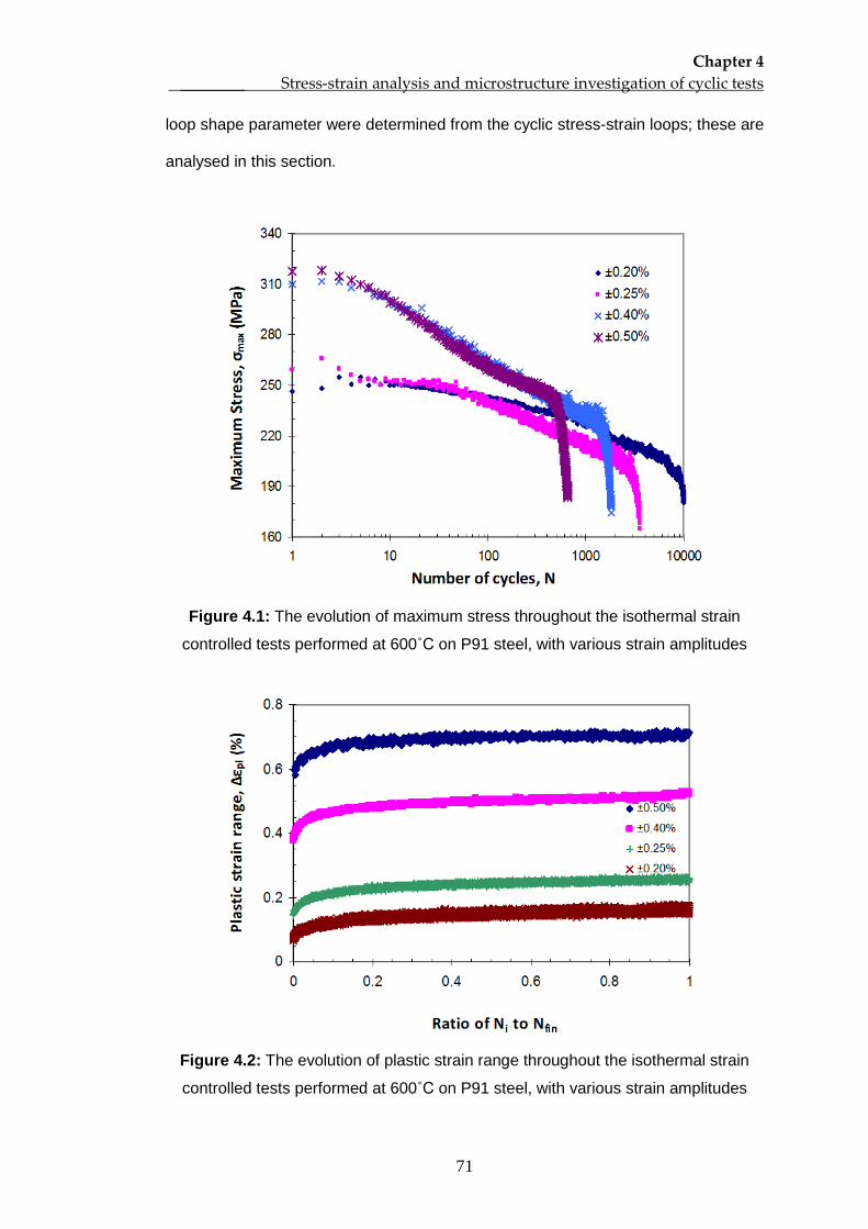
Chapter 4 ________ Stress-strain analysis and microstructure investigation of cyclic tests
71
loop shape parameter were determined from the cyclic stress-strain loops; these are
analysed in this section.
Figure 4.1: The evolution of maximum stress throughout the isothermal strain
controlled tests performed at 600˚C on P91 steel, with various strain amplitudes
Figure 4.2: The evolution of plastic strain range throughout the isothermal strain
controlled tests performed at 600˚C on P91 steel, with various strain amplitudes
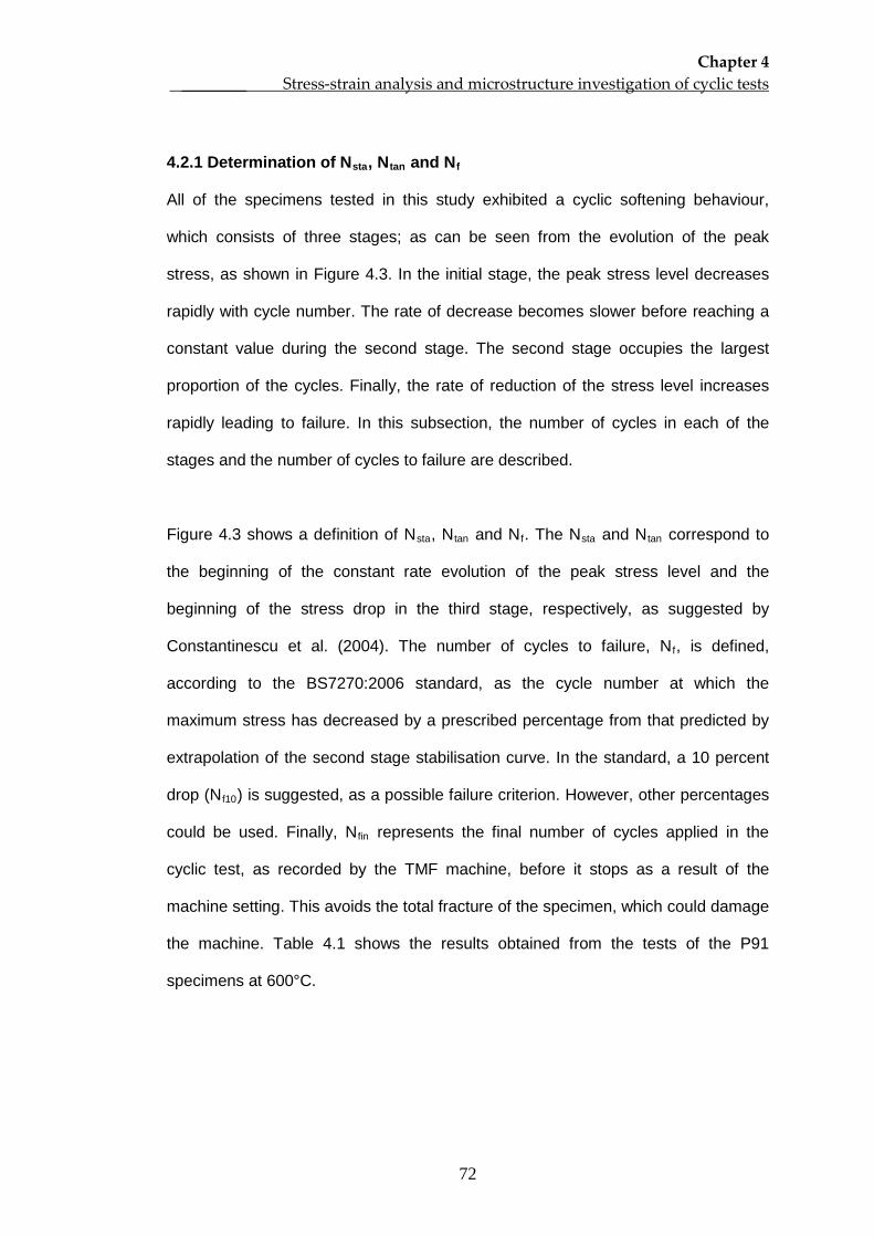
Chapter 4 ________ Stress-strain analysis and microstructure investigation of cyclic tests
72
4.2.1 Determination of Nsta, Ntan and N
All of the specimens tested in this study exhibited a cyclic softening behaviour,
which consists of three stages; as can be seen from the evolution of the peak
stress, as shown in Figure 4.3. In the initial stage, the peak stress level decreases
rapidly with cycle number. The rate of decrease becomes slower before reaching a
constant value during the second stage. The second stage occupies the largest
proportion of the cycles. Finally, the rate of reduction of the stress level increases
rapidly leading to failure. In this subsection, the number of cycles in each of the
stages and the number of cycles to failure are described.
f
Figure 4.3 shows a definition of Nsta, Ntan and Nf. The Nsta and Ntan correspond to
the beginning of the constant rate evolution of the peak stress level and the
beginning of the stress drop in the third stage, respectively, as suggested by
Constantinescu et al. (2004). The number of cycles to failure, Nf, is defined,
according to the BS7270:2006 standard, as the cycle number at which the
maximum stress has decreased by a prescribed percentage from that predicted by
extrapolation of the second stage stabilisation curve. In the standard, a 10 percent
drop (Nf10) is suggested, as a possible failure criterion. However, other percentages
could be used. Finally, Nfin
represents the final number of cycles applied in the
cyclic test, as recorded by the TMF machine, before it stops as a result of the
machine setting. This avoids the total fracture of the specimen, which could damage
the machine. Table 4.1 shows the results obtained from the tests of the P91
specimens at 600°C.
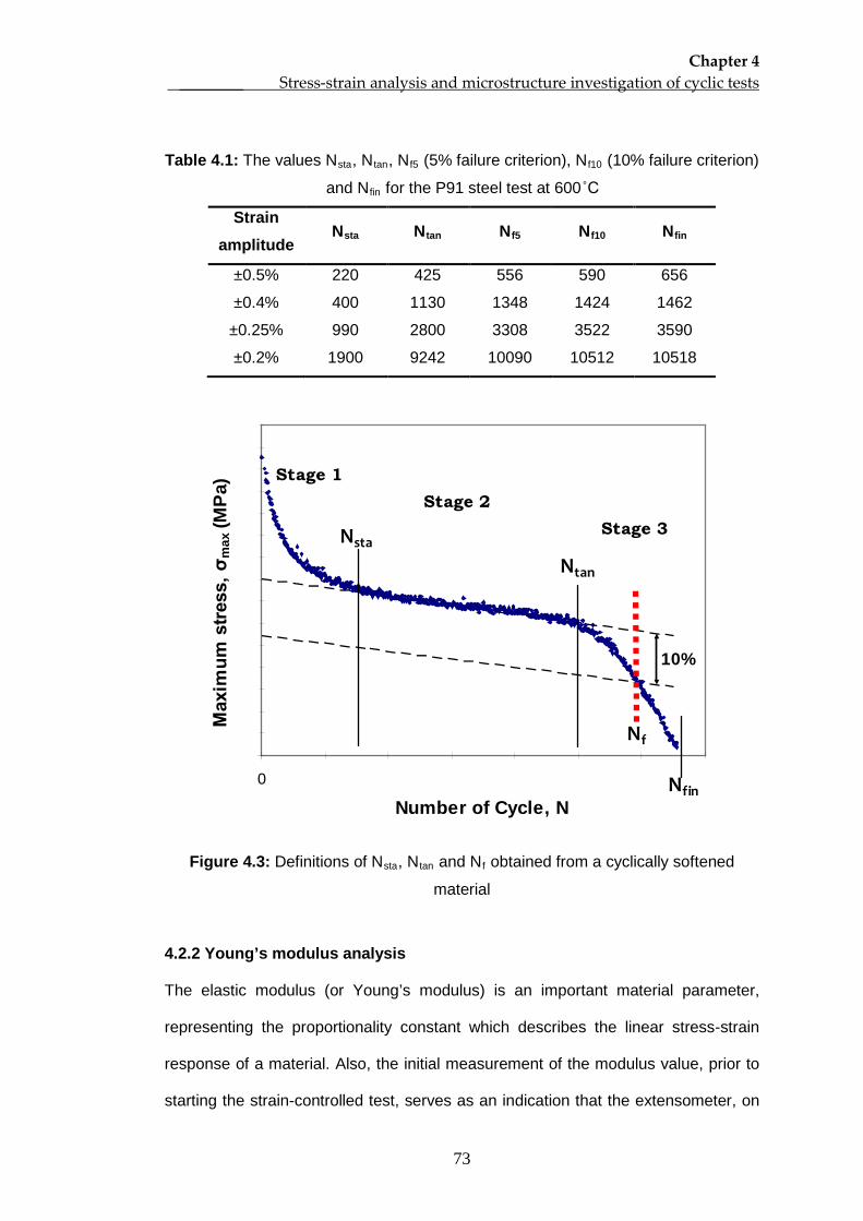
Chapter 4 ________ Stress-strain analysis and microstructure investigation of cyclic tests
73
Table 4.1: The values Nsta, Ntan, Nf5 (5% failure criterion), Nf10 (10% failure criterion)
and Nfin
Strain amplitude
for the P91 steel test at 600˚C
N Nsta Ntan Nf5 Nf10 fin
±0.5% 220 425 556 590 656
±0.4% 400 1130 1348 1424 1462
±0.25% 990 2800 3308 3522 3590
±0.2% 1900 9242 10090 10512 10518
0
Number of Cycle, N
Max
imum
stre
ss, σ
max
(MPa
)
10%
Nf
Stage 1Stage 2
Stage 3Nsta
Ntan
Nfin
Figure 4.3: Definitions of Nsta, Ntan and Nf
obtained from a cyclically softened
material
4.2.2 Young’s modulus analysis
The elastic modulus (or Young’s modulus) is an important material parameter,
representing the proportionality constant which describes the linear stress-strain
response of a material. Also, the initial measurement of the modulus value, prior to
starting the strain-controlled test, serves as an indication that the extensometer, on
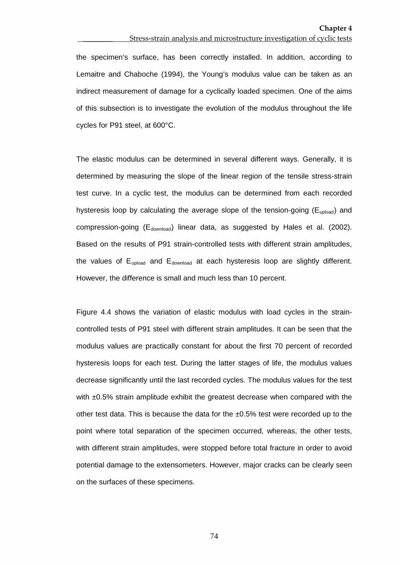
Chapter 4 ________ Stress-strain analysis and microstructure investigation of cyclic tests
74
the specimen’s surface, has been correctly installed. In addition, according to
Lemaitre and Chaboche (1994), the Young’s modulus value can be taken as an
indirect measurement of damage for a cyclically loaded specimen. One of the aims
of this subsection is to investigate the evolution of the modulus throughout the life
cycles for P91 steel, at 600°C.
The elastic modulus can be determined in several different ways. Generally, it is
determined by measuring the slope of the linear region of the tensile stress-strain
test curve. In a cyclic test, the modulus can be determined from each recorded
hysteresis loop by calculating the average slope of the tension-going (Eupload) and
compression-going (Edownload) linear data, as suggested by Hales et al. (2002).
Based on the results of P91 strain-controlled tests with different strain amplitudes,
the values of Eupload and Edownload
at each hysteresis loop are slightly different.
However, the difference is small and much less than 10 percent.
Figure 4.4 shows the variation of elastic modulus with load cycles in the strain-
controlled tests of P91 steel with different strain amplitudes. It can be seen that the
modulus values are practically constant for about the first 70 percent of recorded
hysteresis loops for each test. During the latter stages of life, the modulus values
decrease significantly until the last recorded cycles. The modulus values for the test
with ±0.5% strain amplitude exhibit the greatest decrease when compared with the
other test data. This is because the data for the ±0.5% test were recorded up to the
point where total separation of the specimen occurred, whereas, the other tests,
with different strain amplitudes, were stopped before total fracture in order to avoid
potential damage to the extensometers. However, major cracks can be clearly seen
on the surfaces of these specimens.
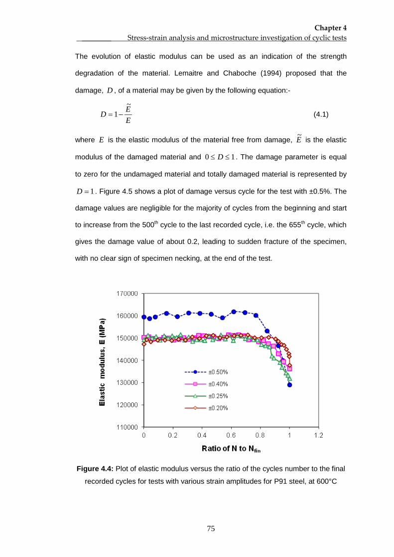
Chapter 4 ________ Stress-strain analysis and microstructure investigation of cyclic tests
75
The evolution of elastic modulus can be used as an indication of the strength
degradation of the material. Lemaitre and Chaboche (1994) proposed that the
damage, D , of a material may be given by the following equation:-
EED~
1−= (4.1)
where E is the elastic modulus of the material free from damage, E~ is the elastic
modulus of the damaged material and 10 ≤≤ D . The damage parameter is equal
to zero for the undamaged material and totally damaged material is represented by
1=D . Figure 4.5 shows a plot of damage versus cycle for the test with ±0.5%. The
damage values are negligible for the majority of cycles from the beginning and start
to increase from the 500th cycle to the last recorded cycle, i.e. the 655th
cycle, which
gives the damage value of about 0.2, leading to sudden fracture of the specimen,
with no clear sign of specimen necking, at the end of the test.
Figure 4.4: Plot of elastic modulus versus the ratio of the cycles number to the final
recorded cycles for tests with various strain amplitudes for P91 steel, at 600°C
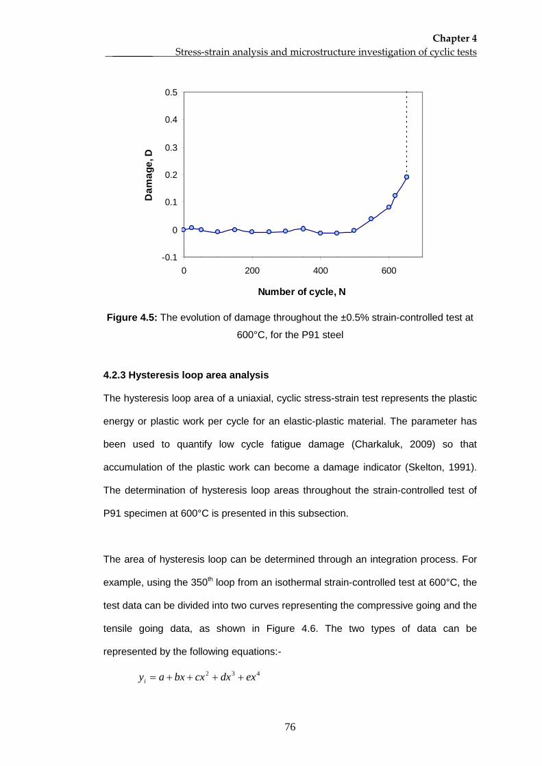
Chapter 4 ________ Stress-strain analysis and microstructure investigation of cyclic tests
76
-0.1
0
0.1
0.2
0.3
0.4
0.5
0 200 400 600
Number of cycle, N
Dam
age,
D
Figure 4.5: The evolution of damage throughout the ±0.5% strain-controlled test at
600°C, for the P91 steel
4.2.3 Hysteresis loop area analysis
The hysteresis loop area of a uniaxial, cyclic stress-strain test represents the plastic
energy or plastic work per cycle for an elastic-plastic material. The parameter has
been used to quantify low cycle fatigue damage (Charkaluk, 2009) so that
accumulation of the plastic work can become a damage indicator (Skelton, 1991).
The determination of hysteresis loop areas throughout the strain-controlled test of
P91 specimen at 600°C is presented in this subsection.
The area of hysteresis loop can be determined through an integration process. For
example, using the 350th
432 exdxcxbxayi ++++=
loop from an isothermal strain-controlled test at 600°C, the
test data can be divided into two curves representing the compressive going and the
tensile going data, as shown in Figure 4.6. The two types of data can be
represented by the following equations:-
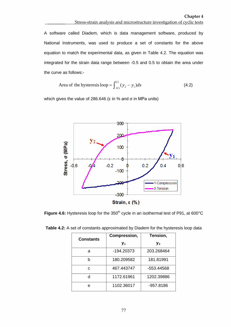
Chapter 4 ________ Stress-strain analysis and microstructure investigation of cyclic tests
77
A software called Diadem, which is data management software, produced by
National Instruments, was used to produce a set of constants for the above
equation to match the experimental data, as given in Table 4.2. The equation was
integrated for the strain data range between -0.5 and 0.5 to obtain the area under
the curve as follows:-
∫− −=5.0
5.0 12 )(loop hysteresis theof Area dxyy (4.2)
which gives the value of 286.646 (ɛ in % and σ in MPa units)
Figure 4.6: Hysteresis loop for the 350th
cycle in an isothermal test of P91, at 600°C
Table 4.2: A set of constants approximated by Diadem for the hysteresis loop data
Constants Compression,
yTension,
y1 2
a -194.20373 203.268464
b 180.209582 181.81991
c 467.443747 -553.44568
d 1172.61961 1202.39886
e 1102.36017 -957.8186
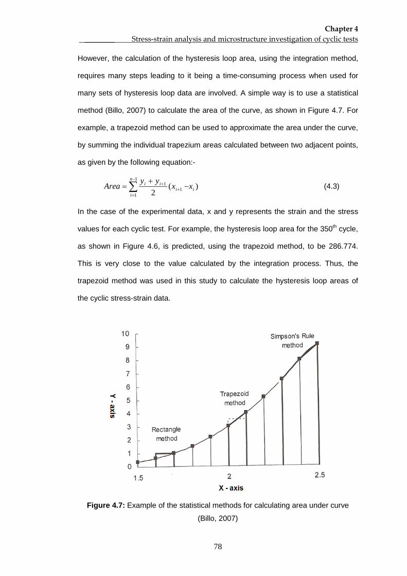
Chapter 4 ________ Stress-strain analysis and microstructure investigation of cyclic tests
78
However, the calculation of the hysteresis loop area, using the integration method,
requires many steps leading to it being a time-consuming process when used for
many sets of hysteresis loop data are involved. A simple way is to use a statistical
method (Billo, 2007) to calculate the area of the curve, as shown in Figure 4.7. For
example, a trapezoid method can be used to approximate the area under the curve,
by summing the individual trapezium areas calculated between two adjacent points,
as given by the following equation:-
)(2
1
11
1i
n
ii
ii xxyy
Area ∑−
=+
+ −+
= (4.3)
In the case of the experimental data, x and y represents the strain and the stress
values for each cyclic test. For example, the hysteresis loop area for the 350th
cycle,
as shown in Figure 4.6, is predicted, using the trapezoid method, to be 286.774.
This is very close to the value calculated by the integration process. Thus, the
trapezoid method was used in this study to calculate the hysteresis loop areas of
the cyclic stress-strain data.
Figure 4.7: Example of the statistical methods for calculating area under curve
(Billo, 2007)
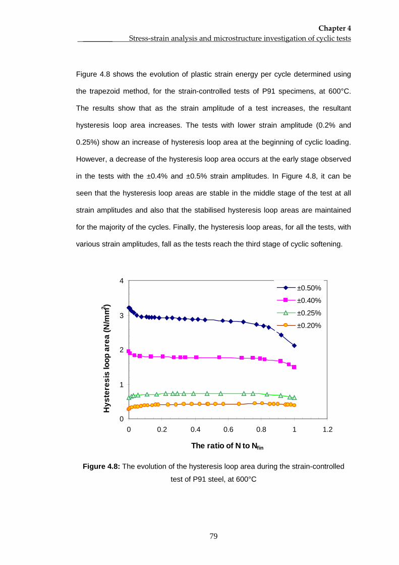
Chapter 4 ________ Stress-strain analysis and microstructure investigation of cyclic tests
79
Figure 4.8 shows the evolution of plastic strain energy per cycle determined using
the trapezoid method, for the strain-controlled tests of P91 specimens, at 600°C.
The results show that as the strain amplitude of a test increases, the resultant
hysteresis loop area increases. The tests with lower strain amplitude (0.2% and
0.25%) show an increase of hysteresis loop area at the beginning of cyclic loading.
However, a decrease of the hysteresis loop area occurs at the early stage observed
in the tests with the ±0.4% and ±0.5% strain amplitudes. In Figure 4.8, it can be
seen that the hysteresis loop areas are stable in the middle stage of the test at all
strain amplitudes and also that the stabilised hysteresis loop areas are maintained
for the majority of the cycles. Finally, the hysteresis loop areas, for all the tests, with
various strain amplitudes, fall as the tests reach the third stage of cyclic softening.
0
1
2
3
4
0 0.2 0.4 0.6 0.8 1 1.2
The ratio of N to Nfin
Hys
tere
sis
loop
are
a (N
/mm2 )
±0.50%
±0.40%
±0.25%
±0.20%
Figure 4.8: The evolution of the hysteresis loop area during the strain-controlled
test of P91 steel, at 600°C
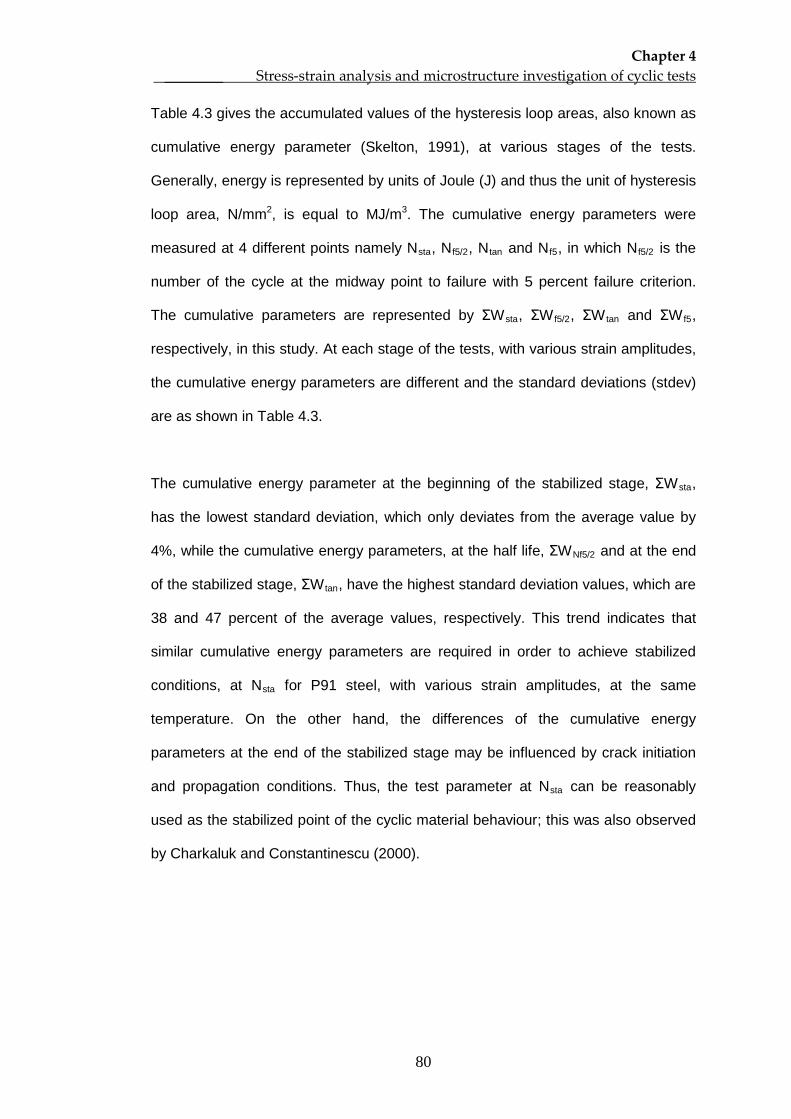
Chapter 4 ________ Stress-strain analysis and microstructure investigation of cyclic tests
80
Table 4.3 gives the accumulated values of the hysteresis loop areas, also known as
cumulative energy parameter (Skelton, 1991), at various stages of the tests.
Generally, energy is represented by units of Joule (J) and thus the unit of hysteresis
loop area, N/mm2, is equal to MJ/m3. The cumulative energy parameters were
measured at 4 different points namely Nsta, Nf5/2, Ntan and Nf5, in which Nf5/2 is the
number of the cycle at the midway point to failure with 5 percent failure criterion.
The cumulative parameters are represented by ΣWsta, ΣWf5/2, ΣWtan and ΣWf5
,
respectively, in this study. At each stage of the tests, with various strain amplitudes,
the cumulative energy parameters are different and the standard deviations (stdev)
are as shown in Table 4.3.
The cumulative energy parameter at the beginning of the stabilized stage, ΣWsta,
has the lowest standard deviation, which only deviates from the average value by
4%, while the cumulative energy parameters, at the half life, ΣWNf5/2 and at the end
of the stabilized stage, ΣWtan, have the highest standard deviation values, which are
38 and 47 percent of the average values, respectively. This trend indicates that
similar cumulative energy parameters are required in order to achieve stabilized
conditions, at Nsta for P91 steel, with various strain amplitudes, at the same
temperature. On the other hand, the differences of the cumulative energy
parameters at the end of the stabilized stage may be influenced by crack initiation
and propagation conditions. Thus, the test parameter at Nsta
can be reasonably
used as the stabilized point of the cyclic material behaviour; this was also observed
by Charkaluk and Constantinescu (2000).
Chapter 4 ________ Stress-strain analysis and microstructure investigation of cyclic tests
81
Table 4.3: The values of cumulative energy parameters of ΣWsta, ΣWf5/2, ΣWtan and
ΣWf5
Strain
amplitude
for the P91 steel test at 600˚C
ΣW ΣWsta ΣWf5/2 ΣWtan f5
±0.5% 648.097 815.206 1233.975 1594.499
±0.4% 720.789 1206.572 2043.090 2311.203
±0.25% 687.036 1167.517 2001.819 2357.516
±0.2% 684.857 1987.211 3774.038 4124.601
Average ΣW 685.195 1294.127 2263.230 2596.955
Stdev 29.702 494.444 1073.732 1076.663
The hysteresis loop areas can be further analysed using a parameter called the loop
shape parameter, HV . The evolution of this parameter throughout the cyclic loading
test indicates the occurrence of persistent slip bands at the surface of the specimen
(Polak, 1991). The HV parameter is given by the following equation:-
aap
HWVσε4
= (4.5)
where W is the hysteresis loop area, apε is the plastic strain amplitude and aσ is
the stress amplitude. Figure 4.9 shows the evolution of loop shape parameter for
the P91 steel specimen subjected to the ±0.5% strain-controlled test. At the
beginning of the test, the HV parameter decreases to a local minimum at about the
40th
cycle. Then, the parameter increases to a local maximum which is located in
the second stage of cyclic softening. Finally, the parameter decreases again in the
final period of testing.
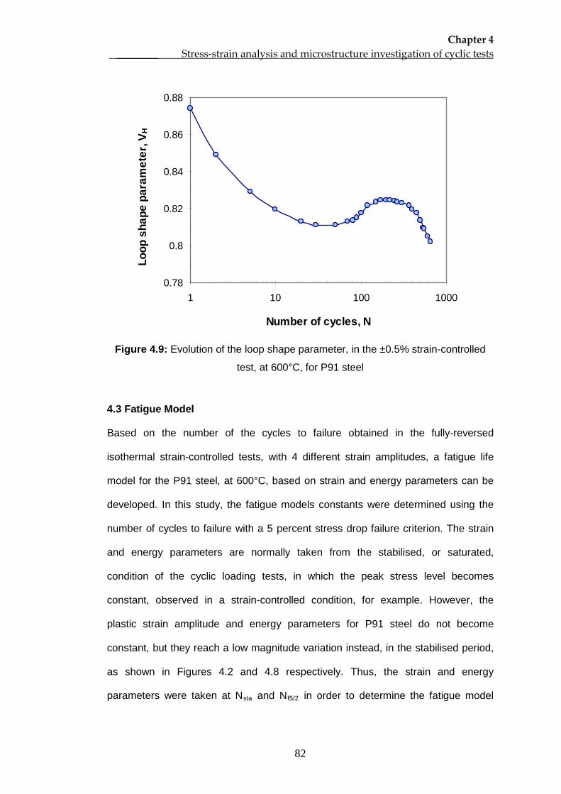
Chapter 4 ________ Stress-strain analysis and microstructure investigation of cyclic tests
82
0.78
0.8
0.82
0.84
0.86
0.88
1 10 100 1000
Number of cycles, N
Loop
sha
pe p
aram
eter
, VH
Figure 4.9: Evolution of the loop shape parameter, in the ±0.5% strain-controlled
test, at 600°C, for P91 steel
4.3 Fatigue Model
Based on the number of the cycles to failure obtained in the fully-reversed
isothermal strain-controlled tests, with 4 different strain amplitudes, a fatigue life
model for the P91 steel, at 600°C, based on strain and energy parameters can be
developed. In this study, the fatigue models constants were determined using the
number of cycles to failure with a 5 percent stress drop failure criterion. The strain
and energy parameters are normally taken from the stabilised, or saturated,
condition of the cyclic loading tests, in which the peak stress level becomes
constant, observed in a strain-controlled condition, for example. However, the
plastic strain amplitude and energy parameters for P91 steel do not become
constant, but they reach a low magnitude variation instead, in the stabilised period,
as shown in Figures 4.2 and 4.8 respectively. Thus, the strain and energy
parameters were taken at Nsta and Nf5/2 in order to determine the fatigue model
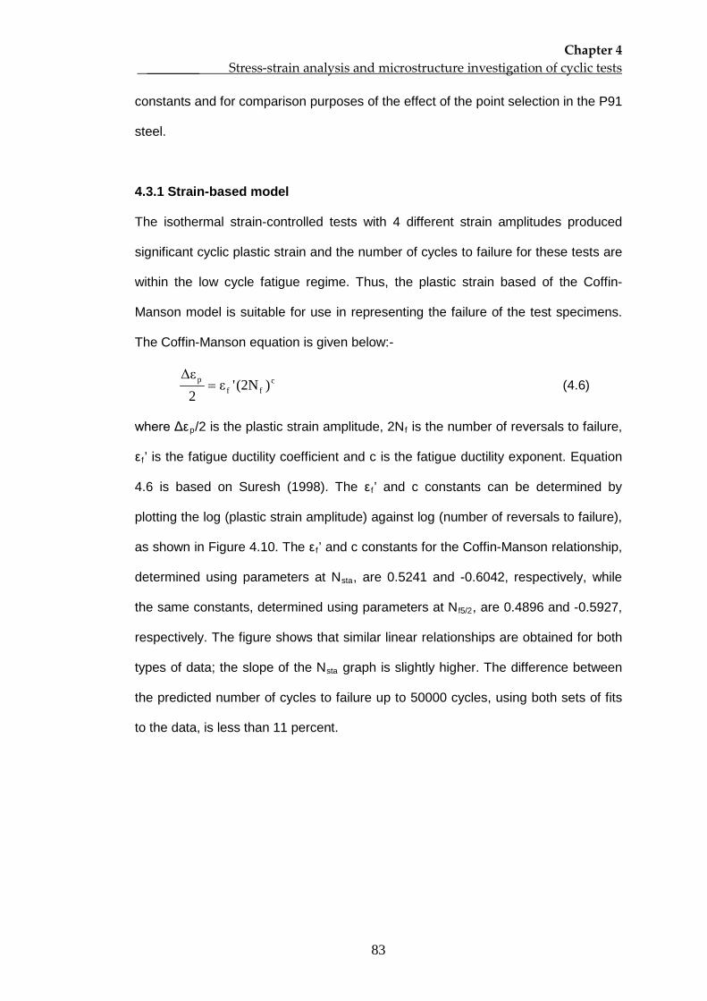
Chapter 4 ________ Stress-strain analysis and microstructure investigation of cyclic tests
83
constants and for comparison purposes of the effect of the point selection in the P91
steel.
4.3.1 Strain-based model
The isothermal strain-controlled tests with 4 different strain amplitudes produced
significant cyclic plastic strain and the number of cycles to failure for these tests are
within the low cycle fatigue regime. Thus, the plastic strain based of the Coffin-
Manson model is suitable for use in representing the failure of the test specimens.
The Coffin-Manson equation is given below:-
cff
p )(2N'ε2Δε
= (4.6)
where Δεp/2 is the plastic strain amplitude, 2Nf is the number of reversals to failure,
ε f’ is the fatigue ductility coefficient and c is the fatigue ductility exponent. Equation
4.6 is based on Suresh (1998). The ε f’ and c constants can be determined by
plotting the log (plastic strain amplitude) against log (number of reversals to failure),
as shown in Figure 4.10. The ε f’ and c constants for the Coffin-Manson relationship,
determined using parameters at Nsta, are 0.5241 and -0.6042, respectively, while
the same constants, determined using parameters at Nf5/2, are 0.4896 and -0.5927,
respectively. The figure shows that similar linear relationships are obtained for both
types of data; the slope of the Nsta
graph is slightly higher. The difference between
the predicted number of cycles to failure up to 50000 cycles, using both sets of fits
to the data, is less than 11 percent.
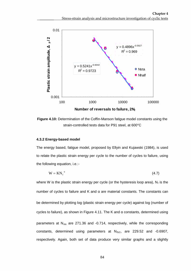
Chapter 4 ________ Stress-strain analysis and microstructure investigation of cyclic tests
84
y = 0.5241x-0.6042
R2 = 0.9723
y = 0.4896x-0.5927
R2 = 0.969
0.001
0.01
100 1000 10000 100000
Number of reversals to failure, 2Nf
Plas
tic s
trai
n am
plitu
de, Δ
p / 2
Nsta
Nhalf
Figure 4.10: Determination of the Coffin-Manson fatigue model constants using the
strain-controlled tests data for P91 steel, at 600°C
4.3.2 Energy-based model
The energy based, fatigue model, proposed by Ellyin and Kujawski (1984), is used
to relate the plastic strain energy per cycle to the number of cycles to failure, using
the following equation, i.e.:-
αfKNW = (4.7)
where W is the plastic strain energy per cycle (or the hysteresis loop area), Nf is the
number of cycles to failure and K and α are material constants. The constants can
be determined by plotting log (plastic strain energy per cycle) against log (number of
cycles to failure), as shown in Figure 4.11. The K and α constants, determined using
parameters at Nsta are 271.36 and -0.714, respectively, while the corresponding
constants, determined using parameters at Nf5/2, are 229.52 and -0.6907,
respectively. Again, both set of data produce very similar graphs and a slightly
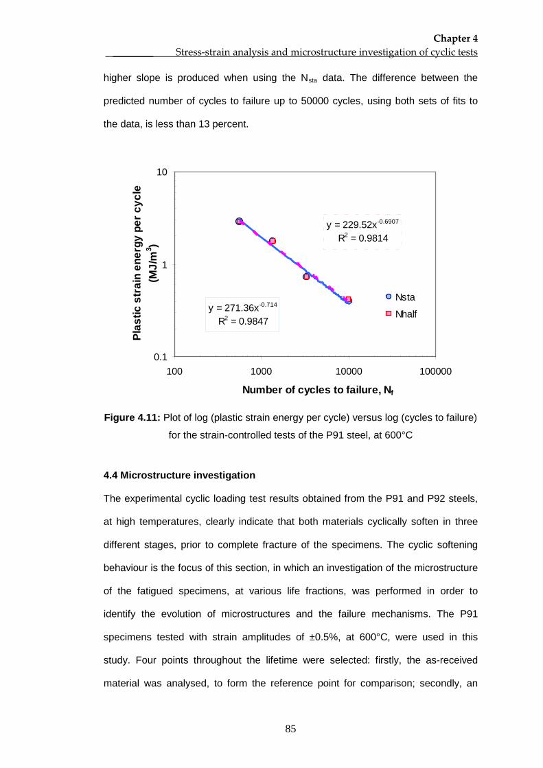
Chapter 4 ________ Stress-strain analysis and microstructure investigation of cyclic tests
85
higher slope is produced when using the Nsta
data. The difference between the
predicted number of cycles to failure up to 50000 cycles, using both sets of fits to
the data, is less than 13 percent.
y = 271.36x-0.714
R2 = 0.9847
y = 229.52x-0.6907
R2 = 0.9814
0.1
1
10
100 1000 10000 100000
Number of cycles to failure, Nf
Plas
tic s
trai
n en
ergy
per
cyc
le
(MJ/
m3 )
Nsta
Nhalf
Figure 4.11: Plot of log (plastic strain energy per cycle) versus log (cycles to failure)
for the strain-controlled tests of the P91 steel, at 600°C
4.4 Microstructure investigation
The experimental cyclic loading test results obtained from the P91 and P92 steels,
at high temperatures, clearly indicate that both materials cyclically soften in three
different stages, prior to complete fracture of the specimens. The cyclic softening
behaviour is the focus of this section, in which an investigation of the microstructure
of the fatigued specimens, at various life fractions, was performed in order to
identify the evolution of microstructures and the failure mechanisms. The P91
specimens tested with strain amplitudes of ±0.5%, at 600°C, were used in this
study. Four points throughout the lifetime were selected: firstly, the as-received
material was analysed, to form the reference point for comparison; secondly, an
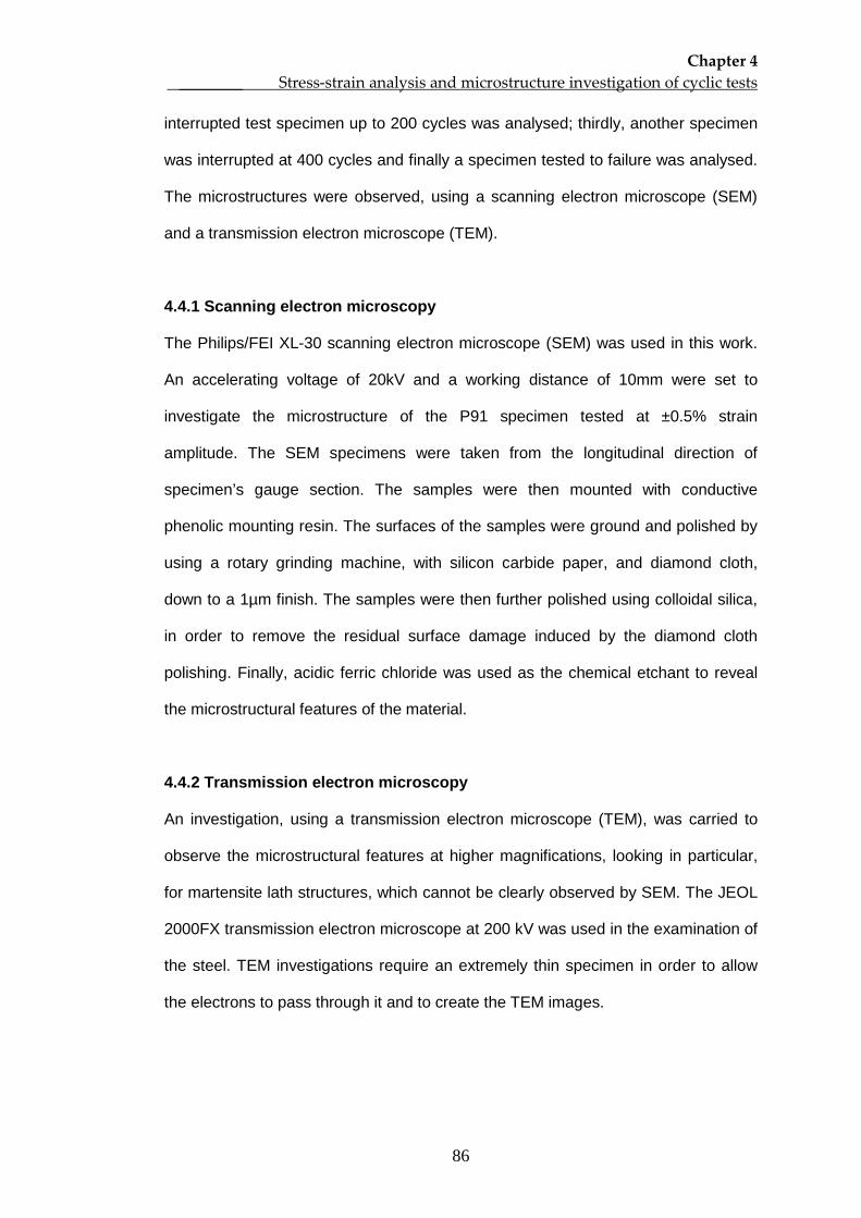
Chapter 4 ________ Stress-strain analysis and microstructure investigation of cyclic tests
86
interrupted test specimen up to 200 cycles was analysed; thirdly, another specimen
was interrupted at 400 cycles and finally a specimen tested to failure was analysed.
The microstructures were observed, using a scanning electron microscope (SEM)
and a transmission electron microscope (TEM).
4.4.1 Scanning electron microscopy
The Philips/FEI XL-30 scanning electron microscope (SEM) was used in this work.
An accelerating voltage of 20kV and a working distance of 10mm were set to
investigate the microstructure of the P91 specimen tested at ±0.5% strain
amplitude. The SEM specimens were taken from the longitudinal direction of
specimen’s gauge section. The samples were then mounted with conductive
phenolic mounting resin. The surfaces of the samples were ground and polished by
using a rotary grinding machine, with silicon carbide paper, and diamond cloth,
down to a 1µm finish. The samples were then further polished using colloidal silica,
in order to remove the residual surface damage induced by the diamond cloth
polishing. Finally, acidic ferric chloride was used as the chemical etchant to reveal
the microstructural features of the material.
4.4.2 Transmission electron microscopy
An investigation, using a transmission electron microscope (TEM), was carried to
observe the microstructural features at higher magnifications, looking in particular,
for martensite lath structures, which cannot be clearly observed by SEM. The JEOL
2000FX transmission electron microscope at 200 kV was used in the examination of
the steel. TEM investigations require an extremely thin specimen in order to allow
the electrons to pass through it and to create the TEM images.
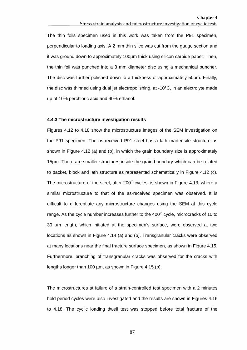
Chapter 4 ________ Stress-strain analysis and microstructure investigation of cyclic tests
87
The thin foils specimen used in this work was taken from the P91 specimen,
perpendicular to loading axis. A 2 mm thin slice was cut from the gauge section and
it was ground down to approximately 100µm thick using silicon carbide paper. Then,
the thin foil was punched into a 3 mm diameter disc using a mechanical puncher.
The disc was further polished down to a thickness of approximately 50µm. Finally,
the disc was thinned using dual jet electropolishing, at -10°C, in an electrolyte made
up of 10% perchloric acid and 90% ethanol.
4.4.3 The microstructure investigation results
Figures 4.12 to 4.18 show the microstructure images of the SEM investigation on
the P91 specimen. The as-received P91 steel has a lath martensite structure as
shown in Figure 4.12 (a) and (b), in which the grain boundary size is approximately
15µm. There are smaller structures inside the grain boundary which can be related
to packet, block and lath structure as represented schematically in Figure 4.12 (c).
The microstructure of the steel, after 200th cycles, is shown in Figure 4.13, where a
similar microstructure to that of the as-received specimen was observed. It is
difficult to differentiate any microstructure changes using the SEM at this cycle
range. As the cycle number increases further to the 400th
cycle, microcracks of 10 to
30 µm length, which initiated at the specimen’s surface, were observed at two
locations as shown in Figure 4.14 (a) and (b). Transgranular cracks were observed
at many locations near the final fracture surface specimen, as shown in Figure 4.15.
Furthermore, branching of transgranular cracks was observed for the cracks with
lengths longer than 100 µm, as shown in Figure 4.15 (b).
The microstructures at failure of a strain-controlled test specimen with a 2 minutes
hold period cycles were also investigated and the results are shown in Figures 4.16
to 4.18. The cyclic loading dwell test was stopped before total fracture of the
Chapter 4 ________ Stress-strain analysis and microstructure investigation of cyclic tests
88
specimen occurred, but one major crack can be clearly seen in Figure 4.16. Many
cracks were initiated from the specimen’s surface, and one major crack (the longest
crack found in the specimen) can be observed in the centre of this figure. The major
crack is about 1 mm in length. Interestingly, microcracks were observed in the
middle of the specimen, as shown in Figure 4.17, but these were not found in the
test specimen without the hold period. Figure 4.18 shows a close-up found in the
major cracks of the P91 dwell specimen; there were cracks which were found to
grow around the grain boundaries. This may indicate the interaction of the creep
and fatigue effects in the crack propagation stage.
Figures 4.19 (a) to 4.19 (d) show the bright field TEM images at high magnification,
after various life fractions produced in the interrupted cyclic loading test of P91
steel. The martensite lath, or the subgrain structures, can be clearly observed using
the transmission electron microscope. For the as-received P91 specimen (zero
cycle), the width of the subgrain are inconsistent, as shown in Figure 4.19 (a), and
small subgrains were observed as highlighted by the dotted line. As the cycle
number increases, the small subgrains become harder to observe in the TEM
images, as can be seen in Figures 4.19 (b) to 4.19 (d). Also, the subgrains, or lath
martensite structures, seem to have a longer structure than does the as-received
subgrain structure. The average of the subgrain width or the subgrain size can be
determined by the line intersection technique as the average of subgrain intercept
lengths measured from the TEM images (Dubey et al., 2005). Based on the bright
field TEM images, the subgrain sizes for Figures 4.19 (a) to 4.19 (d) are 0.383,
0.507, 0.551 and 0.604 µm, respectively. The subgrain size of 200th cycle specimen
increases by about 32 percent from the size of the as-received specimen. Then, the
subgrain sizes increase gradually up to fracture. From these results, there is a clear
trend of subgrain coarsening as the number of cycles increase.
Chapter 4 ________ Stress-strain analysis and microstructure investigation of cyclic tests
89
Figure 4.12: Microstructure of the as-received P91 steel showing (a) the lath
martensite structure, (b) the microstructure at higher magnification for the dotted
circle in (a), and (c) the schematic structure (Kitahara et al, 2006)
(a)
(b)
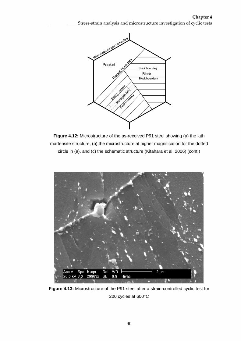
Chapter 4 ________ Stress-strain analysis and microstructure investigation of cyclic tests
90
Figure 4.12: Microstructure of the as-received P91 steel showing (a) the lath
martensite structure, (b) the microstructure at higher magnification for the dotted
circle in (a), and (c) the schematic structure (Kitahara et al, 2006) (cont.)
Figure 4.13: Microstructure of the P91 steel after a strain-controlled cyclic test for
200 cycles at 600°C
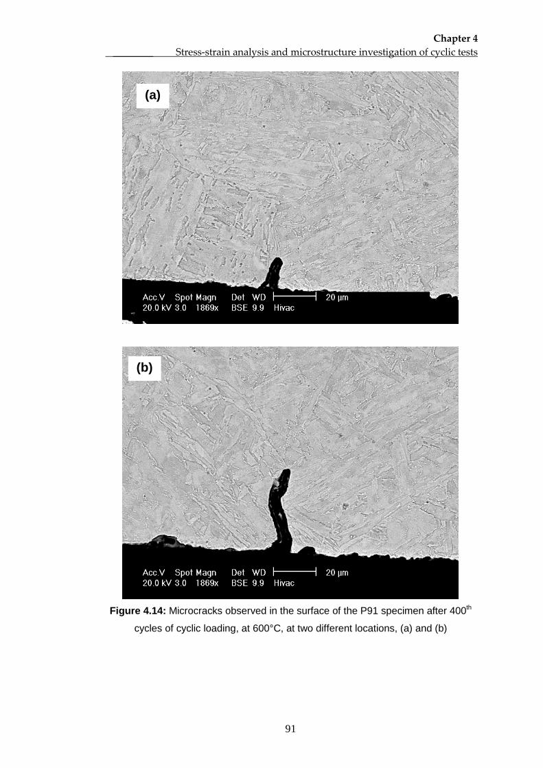
Chapter 4 ________ Stress-strain analysis and microstructure investigation of cyclic tests
91
Figure 4.14: Microcracks observed in the surface of the P91 specimen after 400th
cycles of cyclic loading, at 600°C, at two different locations, (a) and (b)
(a)
(b)
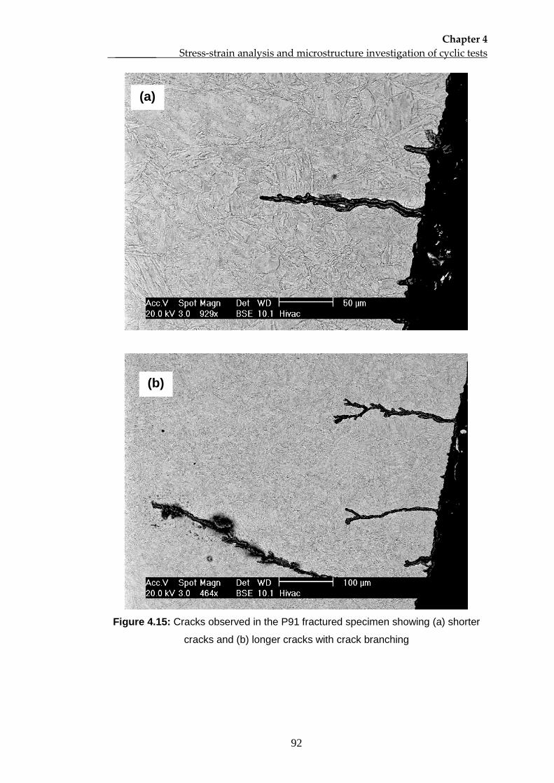
Chapter 4 ________ Stress-strain analysis and microstructure investigation of cyclic tests
92
Figure 4.15: Cracks observed in the P91 fractured specimen showing (a) shorter
cracks and (b) longer cracks with crack branching
(a)
(b)
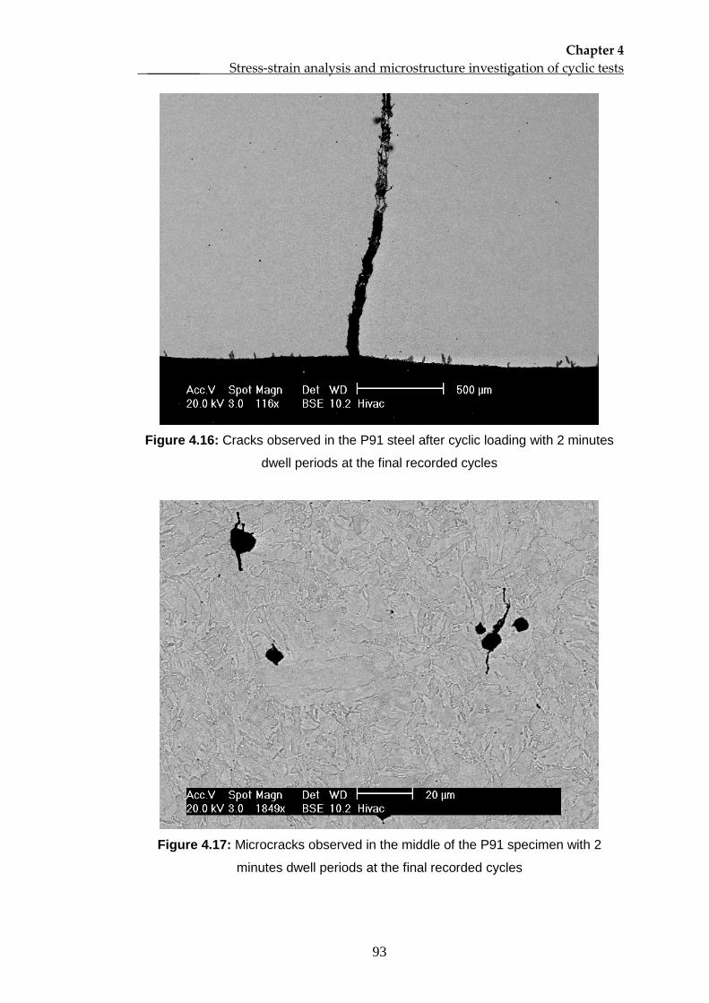
Chapter 4 ________ Stress-strain analysis and microstructure investigation of cyclic tests
93
Figure 4.16: Cracks observed in the P91 steel after cyclic loading with 2 minutes
dwell periods at the final recorded cycles
Figure 4.17: Microcracks observed in the middle of the P91 specimen with 2
minutes dwell periods at the final recorded cycles
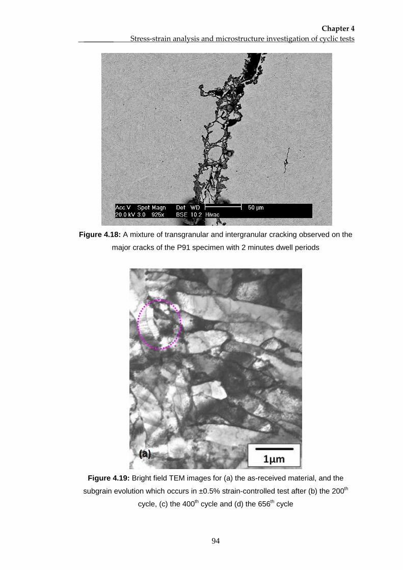
Chapter 4 ________ Stress-strain analysis and microstructure investigation of cyclic tests
94
Figure 4.18: A mixture of transgranular and intergranular cracking observed on the
major cracks of the P91 specimen with 2 minutes dwell periods
Figure 4.19: Bright field TEM images for (a) the as-received material, and the
subgrain evolution which occurs in ±0.5% strain-controlled test after (b) the 200th
cycle, (c) the 400th cycle and (d) the 656th cycle

Chapter 4 ________ Stress-strain analysis and microstructure investigation of cyclic tests
95
Figure 4.19: Bright field TEM images for (a) the as-received material, and the
subgrain evolution which occurs in ±0.5% strain-controlled test after (b) the 200th
cycle, (c) the 400th cycle and (d) 656th cycle
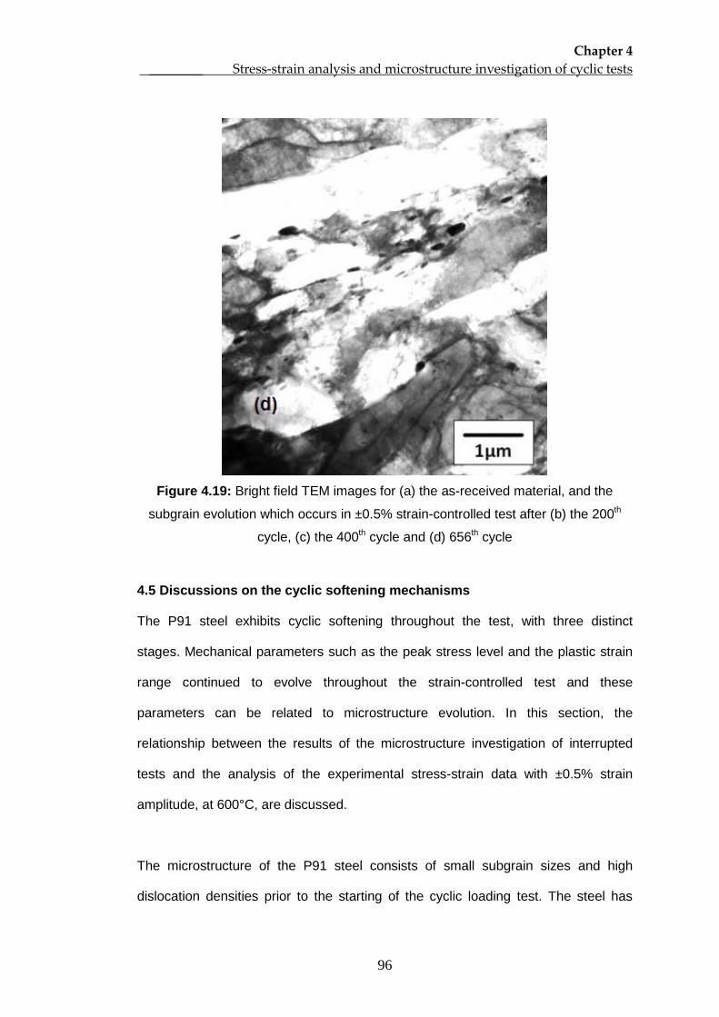
Chapter 4 ________ Stress-strain analysis and microstructure investigation of cyclic tests
96
Figure 4.19: Bright field TEM images for (a) the as-received material, and the
subgrain evolution which occurs in ±0.5% strain-controlled test after (b) the 200th
cycle, (c) the 400th cycle and (d) 656th
cycle
4.5 Discussions on the cyclic softening mechanisms
The P91 steel exhibits cyclic softening throughout the test, with three distinct
stages. Mechanical parameters such as the peak stress level and the plastic strain
range continued to evolve throughout the strain-controlled test and these
parameters can be related to microstructure evolution. In this section, the
relationship between the results of the microstructure investigation of interrupted
tests and the analysis of the experimental stress-strain data with ±0.5% strain
amplitude, at 600°C, are discussed.
The microstructure of the P91 steel consists of small subgrain sizes and high
dislocation densities prior to the starting of the cyclic loading test. The steel has
Chapter 4 ________ Stress-strain analysis and microstructure investigation of cyclic tests
97
been manufactured with these features included as parts of the strengthening
mechanisms of the steel; these act as obstacles to plastic deformation (Abe, 2008).
During the first stage of the cyclic softening of the steel, the peak stress level and
the plastic strain range vary significantly. Also, in this stage, the microstructure
evolution has occurred, particularly in the martensite lath, or subgrain, structure,
without affecting the strength of the specimen, as indicated by the Young’s modulus
values. The results of the TEM investigation show rapid subgrain coarsening during
this stage. At the same time, the dislocation density also decreases due to cyclic
deformation, as reported by Fournier et al. (2009b) for a similar material, at high
temperature. The subgrain coarsening is attributed to the annihilation of low angle
boundaries, as explained by Sauzay et al. (2005). The author reports that the
misorientation angles between laths (or subgrains) are low (smaller than 5°) and
that they can be modelled as dislocation arrays. During plastic deformation, mobile
dislocations move towards low angle boundaries of opposite signs and the
interactions between the opposite signs of dislocations cause the dislocations to be
annihilated. As the cycle number continues to increase the dislocations inside the
subgrains decrease and finally contribute to the disappearance of the low angle
boundaries. Consequently, the subgrain size coarsens and the density of the
dislocations decreases, which means that there is a reduction of the number of
obstacles to plastic deformation. Thus, lower stresses are required to achieve a
certain deformation, as shown by the rapid decrease of the peak stress levels.
In the second stage of cyclic softening, the peak stresses and the plastic strain
ranges slowly and steadily change with an almost constant rate of peak stress
reduction. The subgrain structures, between the 200th and the 400th cycles, also
show a slight increase in the subgrain size, which may indicate a slow rate for the
annihilation process. The stabilisation of the cyclic stress-strain response may
Chapter 4 ________ Stress-strain analysis and microstructure investigation of cyclic tests
98
indicate the formation of persistence slip bands (PSBs) (Kruml and Polak, 2001).
Based on Figure 4.9, the loop shape parameter reaches global maximum at some
point between the 200th and the 300th cycle, which corresponds to the formation of a
microstructure with PSBs (Petrenec et al., 2011). In this stage, microcracks initiate
without affecting the strength of the specimen, as the size of cracks are small, as
shown by the SEM results at the 400th
cycle.
During the third and final stage of cyclic softening there is a nonlinear decrease of
the peak stress level. In this period, the plastic strain range and the subgrain size
have slightly increased. However, it is clear that during this stage the microcracks,
which were observed at the end of the second stage, continue to propagate. The
SEM images of failed specimens show transgranular cracking with crack branching.
Similar crack observations have been found by Nagesha et al. (2002) for the
modified 9Cr-1Mo steel, at the same temperature. The authors relate the branching
of the transgranular cracks to the high strain amplitudes of testing. As the size of
cracks becomes larger, they affect the Young’s modulus value of the material,
leading to a reduction of modulus value. This can be attributed to a degradation of
strength of the material, as shown by the evolution of damage, D, in Figure 4.5. As
the material becomes weaker, lower stresses are required to achieve the targeted
strains in the cyclic testing specimens.
4.6 Conclusions
The following conclusions can be drawn from the analysis of the stress-strain data
and the microstructure investigation:-
• Three distinct stages of cyclic softening have been identified from the full
cycle data of the P91 cyclic tests.
Chapter 4 ________ Stress-strain analysis and microstructure investigation of cyclic tests
99
• The cumulative energy parameters obtained for the cyclic tests with different
strain amplitudes were found to be similar at the beginning of the
stabilisation stage of cyclic softening.
• The coarsening of the subgrains occurs rapidly in the first stage of cyclic
softening but slows down in the second and third stages.
• The nonlinear decrease of the peak stress level in the first stage is due to a
reduction of the number of obstacles to plastic deformation, as a result of
subgrain coarsening.
• The cyclic mechanical parameters become stabilised in the second stage of
cyclic softening. Also, the initiation of cracks begins in this stage. The
changes of structure, on a micro-scale, do not significantly affect the
strength of the specimen, as the Young’s modulus values of the specimen
remain approximately constant up to the end of the stage 2 cyclic softening.
• The nonlinear decrease of the peak stress level, which occurs in the third
stage, is due to crack propagation. The cracks cause the material to become
weaker, as indicated by the decrease of Young’s modulus value.
• Transgranular cracks were found in the fractured specimen of the strain-
controlled test of ±0.5% strain amplitude, with a 0.1%/s strain rate. This
indicates that the strain rate used in this test can produce purely fatigue
condition.
• The introduction of a 2 minutes hold period, in the tension-compression test,
produces a mixture of transgranular and intergranular type of cracks,
indicating a creep-fatigue interaction effect.
Chapter 5 Viscoplasticity model development
100
Chapter 5 - Viscoplasticity model development
5.1 Overview
This chapter presents the development of the material constitutive models for P91
and P92 steels, under cyclic loading conditions, at high temperature. The results of
the isothermal, strain-controlled, tests are presented in Chapter 3; these show the
cyclic softening and stress relaxation behaviour which occurs in the steels. The
results in Chapter 3 are used extensively in this chapter in order to develop the
material models. A viscoplasticity model has been selected to represent the cyclic
plasticity and the time dependent behaviour of the materials. The material constants
were initially determined by using a step by step procedure and then the constants
were improved by using an optimisation program developed in Matlab in order to
obtain better stress-strain predictions. In the end, the model was further improved
by modifying it to include linear cyclic softening predictions resulting in better stress
evolution predictions up to the end of the secondary stage of cyclic softening.
5.2 The viscoplasticity model
The Chaboche, unified, viscoplasticity model was chosen to model the cyclic
behaviour of the P91 and P92 steels. The model is a time-dependent plasticity
model which includes the effects of isotropic and kinematic hardening as well as the
rate dependency effects associated with creep. The model is called a unified
viscoplasticity model for two reasons: there is no partitioning of the inelastic strain
into plastic and creep strain components; and the hardening rules, which are
isotropic and kinematic hardening, are chosen to be similar to the time-independent
case (Chaboche, 1989). The inelastic strain is also called a viscoplastic strain;
however the former term is used in this study.
Chapter 5 Viscoplasticity model development
101
The inelastic strain rate, pε , of the model are given by the following equations:-
χ)sgn(σZ
εn
p −=f
(5.1)
<=>
=0 x1,-0 x0,0 x1,
sgn(x) and
≤>
=0x 0,0x x,
x (5.2)
kRχσ −−−=f (5.3)
where Z and n are material constants; σ is the applied stress; f is the yield
function; k is the initial cyclic yield stress, also known as the initial elastic limit,
representing the initial size of the yield surface in a deviatoric plane; χ is the
kinematic hardening parameter, also known as the back stress; and R is the
isotropic hardening parameter, also known as the drag stress (Chaboche and
Rousselier, 1983).
The kinematic hardening model is used to express the behaviour of non-
proportional monotonic or cyclic loadings (Chaboche, 2008). In a deviatoric stress
plane, the kinematic hardening represents a translation of yield surface. Its
behaviour is described by the following equation:-
)pχε(aCχ ipiii −= (5.4)
∑=
=M
1iiχχ (5.5)
where i=1,2,…,M ; p is the accumulated inelastic strain; ai and Ci
iχ
represent the
stationary values of and the speed to reach the stationary values, respectively.
The use of more than one back stress (Equation 5.4) allows a better description of a
the nonlinear behaviour of a material. In this study, it has been chosen that M = 2
which gives the total back stress as follows:-
Chapter 5 Viscoplasticity model development
102
21 χχχ += (5.6)
As the number of cycles increase in a cyclic loading condition, a material may
harden or soften with respect to the plastic flow, often as a function of accumulated
inelastic strain. This behaviour is represented by an expansion or contraction of the
yield surface in the deviatoric stress plane. It is referred to as isotropic hardening
due to the fact that it changes uniformly in all directions, in the stress space (Dunne
and Petrinic, 2005) and is described by the following equation:-
pR)b(QR −= (5.7)
where Q is the asymptotic value of the isotropic variable, R, at the stabilized cyclic
condition and b governs the stabilization speed.
In the combined isotropic and kinematic hardening of a plasticity model, the applied
stress consists of yield stress, drag stress and back stress. Plastic flow occurs when
the yield function is equal to zero. For the viscoplasticity model, the plastic yield limit
is no longer applied and the load point may lie outside the yield surface. This
specific behaviour for the model is represented by a viscous stress, vσ , as follows:-
1/nv pZσ = (5. 8)
Thus, the applied stress can be decomposed as:-
)-E(χ))sgn(σσk(Rχσ pv εε=−+++= (5.9)
The equations described above are in the uniaxial form of the viscoplasticity model
which consists of ten temperature dependent material properties, namely E, k, Q, b,
a1, C1, a2, C2, Z and n. A description of how the constants are determined is given
in the next section, using a step by step procedure and an optimisation approach.
Also, the viscoplasticity model, in the uniaxial form, has been implemented in a
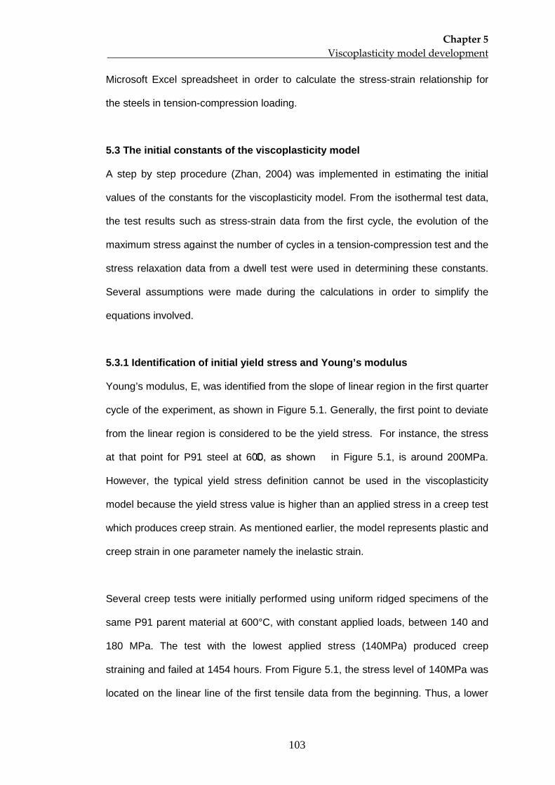
Chapter 5 Viscoplasticity model development
103
Microsoft Excel spreadsheet in order to calculate the stress-strain relationship for
the steels in tension-compression loading.
5.3 The initial constants of the viscoplasticity model
A step by step procedure (Zhan, 2004) was implemented in estimating the initial
values of the constants for the viscoplasticity model. From the isothermal test data,
the test results such as stress-strain data from the first cycle, the evolution of the
maximum stress against the number of cycles in a tension-compression test and the
stress relaxation data from a dwell test were used in determining these constants.
Several assumptions were made during the calculations in order to simplify the
equations involved.
5.3.1 Identification of initial yield stress and Young’s modulus
Young’s modulus, E, was identified from the slope of linear region in the first quarter
cycle of the experiment, as shown in Figure 5.1. Generally, the first point to deviate
from the linear region is considered to be the yield stress. For instance, the stress
at that point for P91 steel at 600˚C, as shown in Figure 5.1, is around 200MPa.
However, the typical yield stress definition cannot be used in the viscoplasticity
model because the yield stress value is higher than an applied stress in a creep test
which produces creep strain. As mentioned earlier, the model represents plastic and
creep strain in one parameter namely the inelastic strain.
Several creep tests were initially performed using uniform ridged specimens of the
same P91 parent material at 600°C, with constant applied loads, between 140 and
180 MPa. The test with the lowest applied stress (140MPa) produced creep
straining and failed at 1454 hours. From Figure 5.1, the stress level of 140MPa was
located on the linear line of the first tensile data from the beginning. Thus, a lower
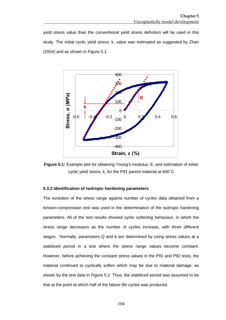
Chapter 5 Viscoplasticity model development
104
yield stress value than the conventional yield stress definition will be used in this
study. The initial cyclic yield stress, k, value was estimated as suggested by Zhan
(2004) and as shown in Figure 5.1.
-400
-300
-200
-100
0
100
200
300
400
-0.6 -0.4 -0.2 0 0.2 0.4 0.6
Strain, ε (%)
Stre
ss, σ
(MPa
)
E
k
Figure 5.1: Example plot for obtaining Young’s modulus, E, and estimation of initial
cyclic yield stress, k, for the P91 parent material at 600˚C
5.3.2 Identification of isotropic hardening parameters
The evolution of the stress range against number of cycles data obtained from a
tension-compression test was used in the determination of the isotropic hardening
parameters. All of the test results showed cyclic softening behaviour, in which the
stress range decreases as the number of cycles increase, with three different
stages. Normally, parameters Q and b are determined by using stress values at a
stabilized period in a test where the stress range values become constant.
However, before achieving the constant stress values in the P91 and P92 tests, the
material continued to cyclically soften which may be due to material damage, as
shown by the test data in Figure 5.2. Thus, the stabilized period was assumed to be
that at the point at which half of the failure life cycles was produced.
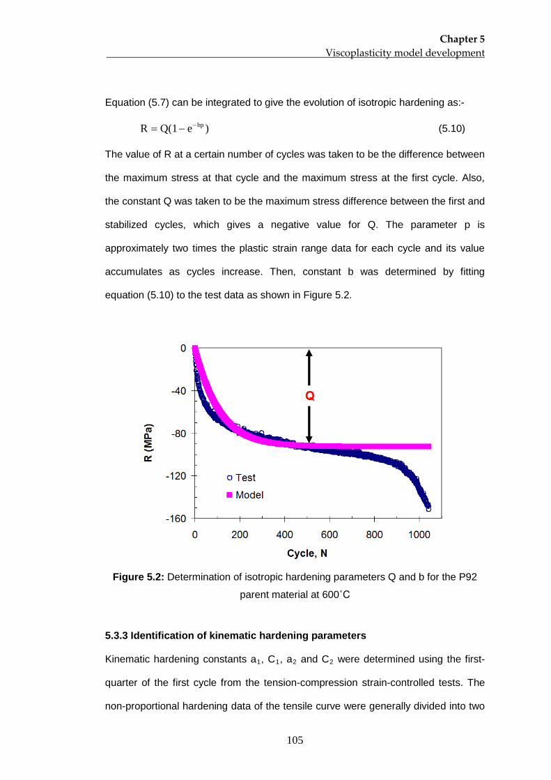
Chapter 5 Viscoplasticity model development
105
Equation (5.7) can be integrated to give the evolution of isotropic hardening as:-
)eQ(1R bp−−= (5.10)
The value of R at a certain number of cycles was taken to be the difference between
the maximum stress at that cycle and the maximum stress at the first cycle. Also,
the constant Q was taken to be the maximum stress difference between the first and
stabilized cycles, which gives a negative value for Q. The parameter p is
approximately two times the plastic strain range data for each cycle and its value
accumulates as cycles increase. Then, constant b was determined by fitting
equation (5.10) to the test data as shown in Figure 5.2.
Figure 5.2: Determination of isotropic hardening parameters Q and b for the P92
parent material at 600˚C
5.3.3 Identification of kinematic hardening parameters
Kinematic hardening constants a1, C1, a2 and C2 were determined using the first-
quarter of the first cycle from the tension-compression strain-controlled tests. The
non-proportional hardening data of the tensile curve were generally divided into two
Chapter 5 Viscoplasticity model development
106
regions, as shown in Figure 5.3, to represent firstly the transient region of the
inelastic deformation, where 1χ becomes the dominant inelasticity contribution, and
secondly the region with greater inelastic strain in which 2χ is the dominant
parameter.
Figure 5.3: Partition of the first quarter of the first cyclic loop for the strain-controlled
test data into an elastic region followed by an inelastic region with 1χ and 2χ
dominated region
Equation (5.4) can be integrated with respect to time to give the following
equations:-
)e(1aχ p-C11
1−= (5.11)
)e(1aχ p-C22
2−= (5.12)
in which pεp = in the first tensile curve data. Equations (5.11) and (5.12) can be
substituted into equation (5.9) to give:-
vεC
2εC
1 σkR)e(1a)e(1aσ p2p1 +++−+−= −− (5.13)
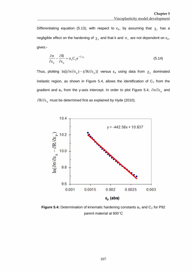
Chapter 5 Viscoplasticity model development
107
Differentiating equation (5.13), with respect to εp 1χ, by assuming that has a
negligible effect on the hardening of 2χ and that k and vσ are not dependent on εp
,
gives:-
p2εC22
pp
eCaεR
εσ −=
∂∂
−∂∂
(5.14)
Thus, plotting )]εR/()εσ/ln[( pp ∂∂−∂∂ versus εp 2χ using data from dominated
inelastic region, as shown in Figure 5.4, allows the identification of C2 from the
gradient and a2 pεσ/∂∂ from the y-axis intercept. In order to plot Figure 5.4, and
pεR/∂∂ must be determined first as explained by Hyde (2010).
Figure 5.4: Determination of kinematic hardening constants a2 and C2
for P92
parent material at 600˚C
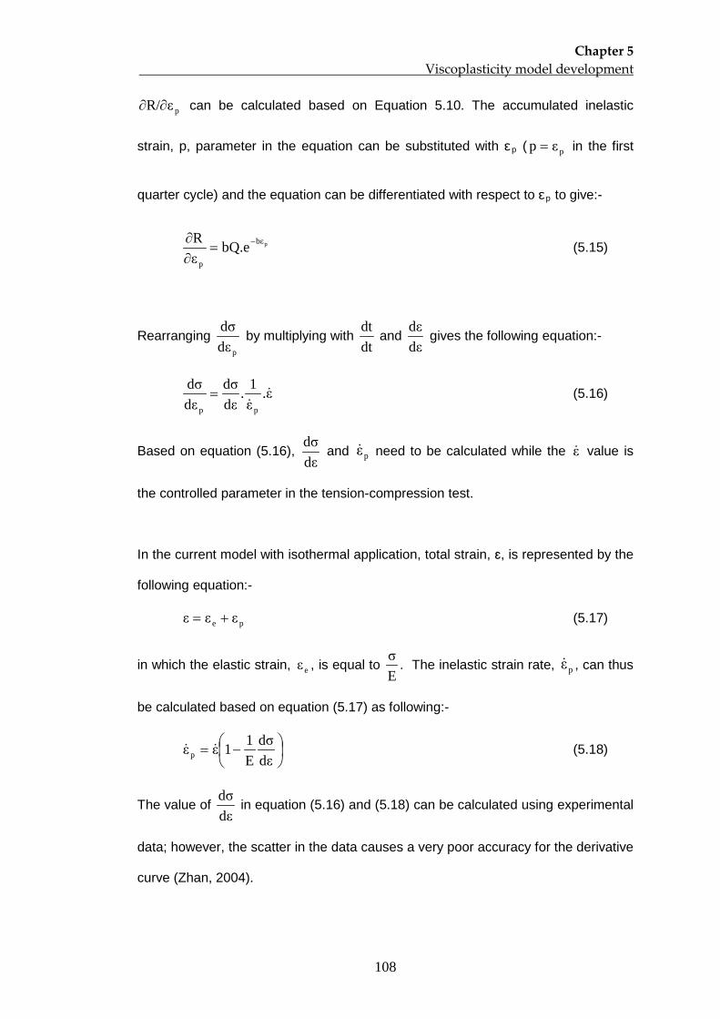
Chapter 5 Viscoplasticity model development
108
pεR/∂∂ can be calculated based on Equation 5.10. The accumulated inelastic
strain, p, parameter in the equation can be substituted with ɛp pεp = ( in the first
quarter cycle) and the equation can be differentiated with respect to ɛp
to give:-
pbε
p
bQ.eεR −=
∂∂
(5.15)
Rearranging pdε
dσ by multiplying with
dtdt
and dεdε
gives the following equation:-
ε.ε1.
dεdσ
dεdσ
pp
= (5.16)
Based on equation (5.16), dεdσ
and pε need to be calculated while the ε value is
the controlled parameter in the tension-compression test.
In the current model with isothermal application, total strain, ɛ, is represented by the
following equation:-
pe εεε += (5.17)
in which the elastic strain, eε , is equal to Eσ
. The inelastic strain rate, pε , can thus
be calculated based on equation (5.17) as following:-
−=
dεdσ
E11εε p (5.18)
The value of dεdσ
in equation (5.16) and (5.18) can be calculated using experimental
data; however, the scatter in the data causes a very poor accuracy for the derivative
curve (Zhan, 2004).
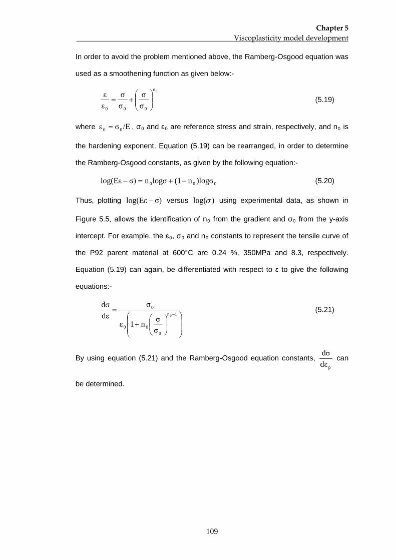
Chapter 5 Viscoplasticity model development
109
In order to avoid the problem mentioned above, the Ramberg-Osgood equation was
used as a smoothening function as given below:-
0n
000 σσ
σσ
εε
+= (5.19)
where /Eσε 00 = , σ0 and ɛ0 are reference stress and strain, respectively, and n0
is
the hardening exponent. Equation (5.19) can be rearranged, in order to determine
the Ramberg-Osgood constants, as given by the following equation:-
000 )logσn(1logσnσ)log(Eε −+=− (5.20)
Thus, plotting σ)log(Eε − versus )log(σ using experimental data, as shown in
Figure 5.5, allows the identification of n0 from the gradient and σ0 from the y-axis
intercept. For example, the ɛ0, σ0 and n0
constants to represent the tensile curve of
the P92 parent material at 600°C are 0.24 %, 350MPa and 8.3, respectively.
Equation (5.19) can again, be differentiated with respect to ɛ to give the following
equations:-
+
=−1n
000
0
0
σσn1ε
σdεdσ
(5.21)
By using equation (5.21) and the Ramberg-Osgood equation constants, pdε
dσ can
be determined.
Chapter 5 Viscoplasticity model development
110
y = 8.3189x - 18.625
0.0
0.5
1.0
1.5
2.0
2.5
3.0
2.25 2.3 2.35 2.4 2.45 2.5 2.55 2.6
log(σ)
log(
E
Figure 5.5: Determination of the Ramberg-Osgood equation constants for P92
parent material at 600°C
On the other hand, as the constants a2 and C2 were obtained previously, equation
(5.13) can be differentiated with respect to ɛp
to give the following equation:-
p1εC11
2
pp
eCaεR
εσ −=
∂∂
−∂∂
−∂∂
pεχ
(5.22)
The constants a1 and C1 1χ, from the dominated inelastic region, can be
determined by plotting )]ε/χ(-)εR/()εσ/ln[( p2pp ∂∂∂∂−∂∂ versus εp
pεσ/∂∂
as shown in
Figure 5.6. Similar procedures to those described earlier, were used to calculate
and pεR/∂∂ for the 1χ dominated inelastic region data.
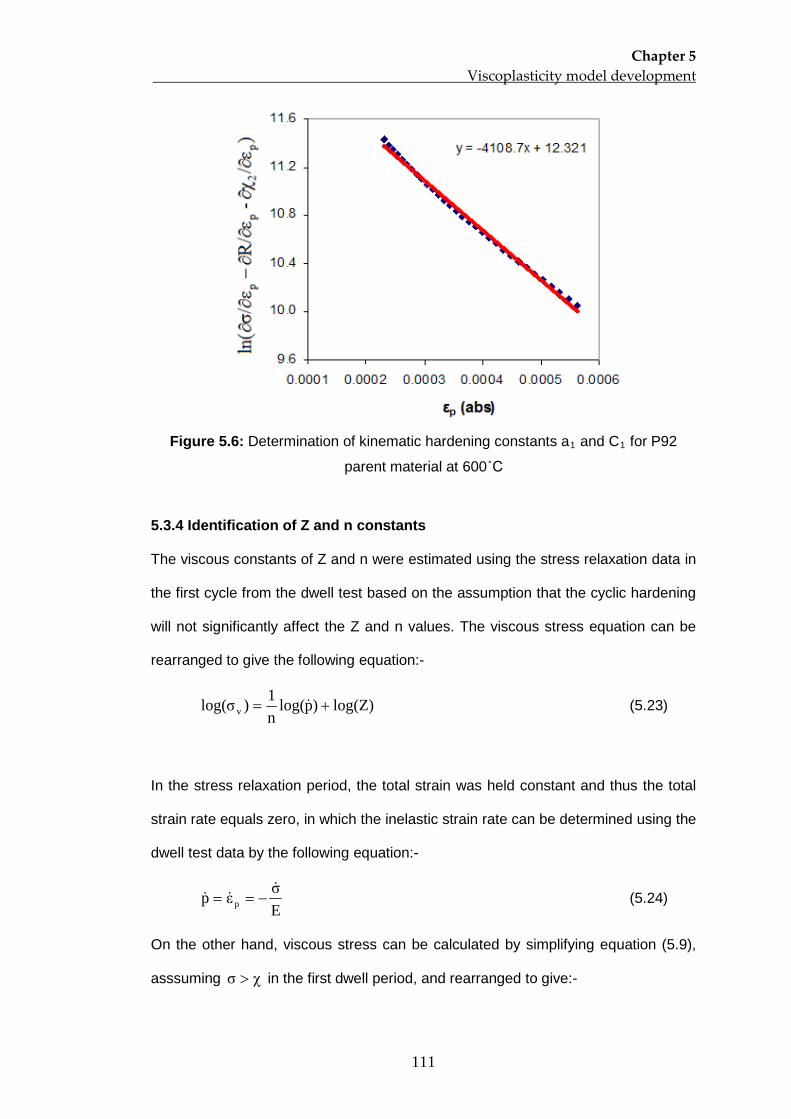
Chapter 5 Viscoplasticity model development
111
Figure 5.6: Determination of kinematic hardening constants a1 and C1
for P92
parent material at 600˚C
5.3.4 Identification of Z and n constants
The viscous constants of Z and n were estimated using the stress relaxation data in
the first cycle from the dwell test based on the assumption that the cyclic hardening
will not significantly affect the Z and n values. The viscous stress equation can be
rearranged to give the following equation:-
log(Z))plog(n1)log(σ v += (5.23)
In the stress relaxation period, the total strain was held constant and thus the total
strain rate equals zero, in which the inelastic strain rate can be determined using the
dwell test data by the following equation:-
Eσεp p
−== (5.24)
On the other hand, viscous stress can be calculated by simplifying equation (5.9),
asssuming χσ > in the first dwell period, and rearranged to give:-
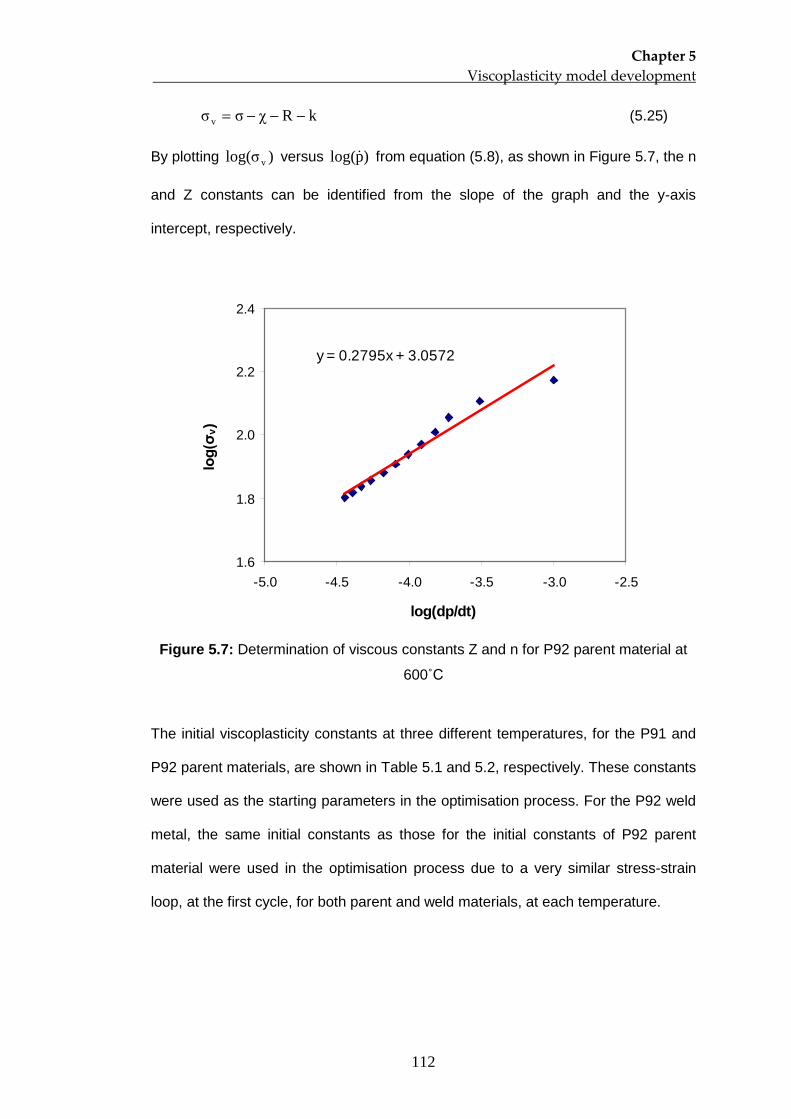
Chapter 5 Viscoplasticity model development
112
kRχσσ v −−−= (5.25)
By plotting )log(σ v versus )plog( from equation (5.8), as shown in Figure 5.7, the n
and Z constants can be identified from the slope of the graph and the y-axis
intercept, respectively.
y = 0.2795x + 3.0572
1.6
1.8
2.0
2.2
2.4
-5.0 -4.5 -4.0 -3.5 -3.0 -2.5
log(dp/dt)
log(
σ v)
Figure 5.7: Determination of viscous constants Z and n for P92 parent material at
600˚C
The initial viscoplasticity constants at three different temperatures, for the P91 and
P92 parent materials, are shown in Table 5.1 and 5.2, respectively. These constants
were used as the starting parameters in the optimisation process. For the P92 weld
metal, the same initial constants as those for the initial constants of P92 parent
material were used in the optimisation process due to a very similar stress-strain
loop, at the first cycle, for both parent and weld materials, at each temperature.
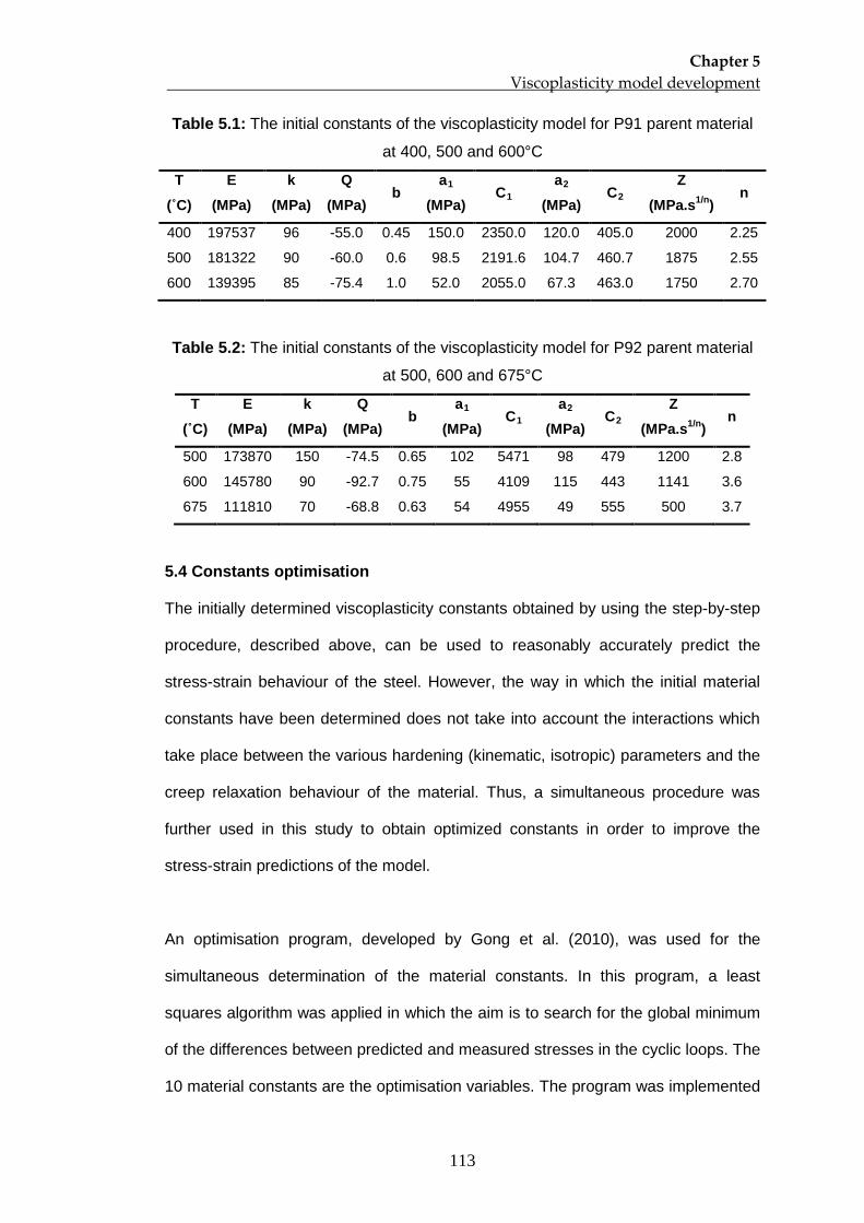
Chapter 5 Viscoplasticity model development
113
Table 5.1: The initial constants of the viscoplasticity model for P91 parent material
at 400, 500 and 600°C
T (˚C)
E (MPa)
k (MPa)
Q (MPa)
b a
(MPa) 1
Ca
1 (MPa)
2 C
Z 2
(MPa.s1/n n )
400 197537 96 -55.0 0.45 150.0 2350.0 120.0 405.0 2000 2.25
500 181322 90 -60.0 0.6 98.5 2191.6 104.7 460.7 1875 2.55
600 139395 85 -75.4 1.0 52.0 2055.0 67.3 463.0 1750 2.70
Table 5.2: The initial constants of the viscoplasticity model for P92 parent material
at 500, 600 and 675°C
T (˚C)
E (MPa)
k (MPa)
Q (MPa)
b a
(MPa) 1
Ca
1 (MPa)
2 C
Z 2
(MPa.s1/n n )
500 173870 150 -74.5 0.65 102 5471 98 479 1200 2.8
600 145780 90 -92.7 0.75 55 4109 115 443 1141 3.6
675 111810 70 -68.8 0.63 54 4955 49 555 500 3.7
5.4 Constants optimisation
The initially determined viscoplasticity constants obtained by using the step-by-step
procedure, described above, can be used to reasonably accurately predict the
stress-strain behaviour of the steel. However, the way in which the initial material
constants have been determined does not take into account the interactions which
take place between the various hardening (kinematic, isotropic) parameters and the
creep relaxation behaviour of the material. Thus, a simultaneous procedure was
further used in this study to obtain optimized constants in order to improve the
stress-strain predictions of the model.
An optimisation program, developed by Gong et al. (2010), was used for the
simultaneous determination of the material constants. In this program, a least
squares algorithm was applied in which the aim is to search for the global minimum
of the differences between predicted and measured stresses in the cyclic loops. The
10 material constants are the optimisation variables. The program was implemented
Chapter 5 Viscoplasticity model development
114
in Matlab using the nonlinear least squares optimisation function lsqnonlin provided
within the Matlab optimisation toolbox. Two different optimisation programs were
developed previously in which the programs were based on different objective
functions. The applications of these programs in determining the viscoplasticity
constants of the P91 and P92 steels are presented below.
5.4.1 Two objective function optimisation
Firstly, the two objective function optimisation program was used in order to obtain
more accurate stress-strain prediction of tension-compression test data. In this
program, two types of data obtained from the isothermal tension-compression test
were used as the objective functions; the first is the stress-strain response and the
other is the evolution of stress range in cyclic softening material which occurs
throughout the test. The optimisation process using the two objective function
program is described in detailed by Hyde (2010) as shown in Figure 5.8.
Several types of inputs were defined in the program prior to starting the optimisation
process. First, the stress-strain data from the isothermal tension-compression tests,
up to the secondary stage of cyclic softening were supplied into the program and
the detail of the test parameters such as the strain rate, ε , the minimum strain, minε
and the maximum strain, minε , were also defined. The lower bound, LB, and the
upper bound, UB, for each of the material constants were set as the searching
boundaries for the viscoplasticity model constants in the optimisation process. The
initial viscoplasticity constants were set as the starting point for the determination of
an optimised constant set.
Some guidelines were used in defining the lower and upper bound of material
constants so that the optimised constants can be a reasonable representation of the
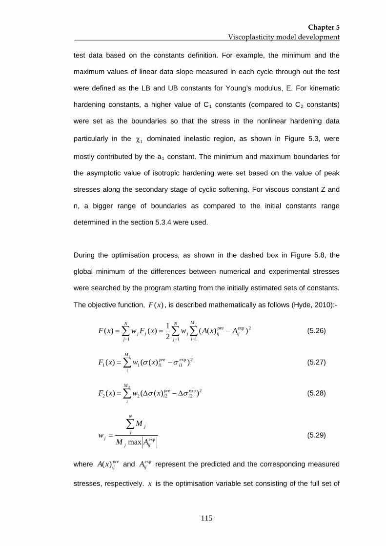
Chapter 5 Viscoplasticity model development
115
test data based on the constants definition. For example, the minimum and the
maximum values of linear data slope measured in each cycle through out the test
were defined as the LB and UB constants for Young’s modulus, E. For kinematic
hardening constants, a higher value of C1 constants (compared to C2
1χ
constants)
were set as the boundaries so that the stress in the nonlinear hardening data
particularly in the dominated inelastic region, as shown in Figure 5.3, were
mostly contributed by the a1
constant. The minimum and maximum boundaries for
the asymptotic value of isotropic hardening were set based on the value of peak
stresses along the secondary stage of cyclic softening. For viscous constant Z and
n, a bigger range of boundaries as compared to the initial constants range
determined in the section 5.3.4 were used.
During the optimisation process, as shown in the dashed box in Figure 5.8, the
global minimum of the differences between numerical and experimental stresses
were searched by the program starting from the initially estimated sets of constants.
The objective function, )(xF , is described mathematically as follows (Hyde, 2010):-
∑∑∑===
−==jM
iij
preij
N
jjj
N
jj AxAwxFwxF
1
2exp
11))((
21)()( (5.26)
2exp1111 ))(()(
1
∑ −=M
ii
preixwxF σσ (5.27)
2exp2222 ))(()(
2
∑ ∆−∆=M
ii
preixwxF σσ (5.28)
expmax ijj
N
jj
j AM
Mw
∑= (5.29)
where preijxA )( and exp
ijA represent the predicted and the corresponding measured
stresses, respectively. x is the optimisation variable set consisting of the full set of
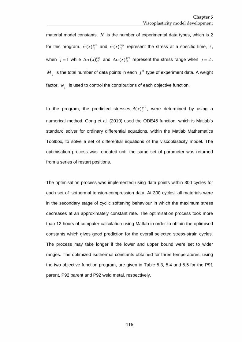
Chapter 5 Viscoplasticity model development
116
material model constants. N is the number of experimental data types, which is 2
for this program. preix 1)(σ and exp
1)( ixσ represent the stress at a specific time, i ,
when 1=j while exp2)( ixσ∆ and pre
ix 2)(σ∆ represent the stress range when 2=j .
jM is the total number of data points in each thj type of experiment data. A weight
factor, jw , is used to control the contributions of each objective function.
In the program, the predicted stresses, preijxA )( , were determined by using a
numerical method. Gong et al. (2010) used the ODE45 function, which is Matlab’s
standard solver for ordinary differential equations, within the Matlab Mathematics
Toolbox, to solve a set of differential equations of the viscoplasticity model. The
optimisation process was repeated until the same set of parameter was returned
from a series of restart positions.
The optimisation process was implemented using data points within 300 cycles for
each set of isothermal tension-compression data. At 300 cycles, all materials were
in the secondary stage of cyclic softening behaviour in which the maximum stress
decreases at an approximately constant rate. The optimisation process took more
than 12 hours of computer calculation using Matlab in order to obtain the optimised
constants which gives good prediction for the overall selected stress-strain cycles.
The process may take longer if the lower and upper bound were set to wider
ranges. The optimized isothermal constants obtained for three temperatures, using
the two objective function program, are given in Table 5.3, 5.4 and 5.5 for the P91
parent, P92 parent and P92 weld metal, respectively.
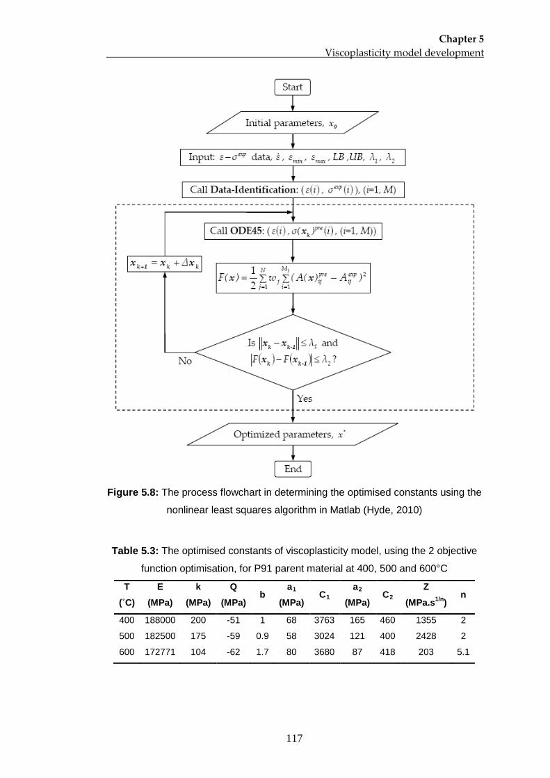
Chapter 5 Viscoplasticity model development
117
Figure 5.8: The process flowchart in determining the optimised constants using the
nonlinear least squares algorithm in Matlab (Hyde, 2010)
Table 5.3: The optimised constants of viscoplasticity model, using the 2 objective
function optimisation, for P91 parent material at 400, 500 and 600°C
T (˚C)
E (MPa)
k (MPa)
Q (MPa)
b a
(MPa) 1
Ca
1 (MPa)
2 C
Z 2
(MPa.s1/n n )
400 188000 200 -51 1 68 3763 165 460 1355 2
500 182500 175 -59 0.9 58 3024 121 400 2428 2
600 172771 104 -62 1.7 80 3680 87 418 203 5.1
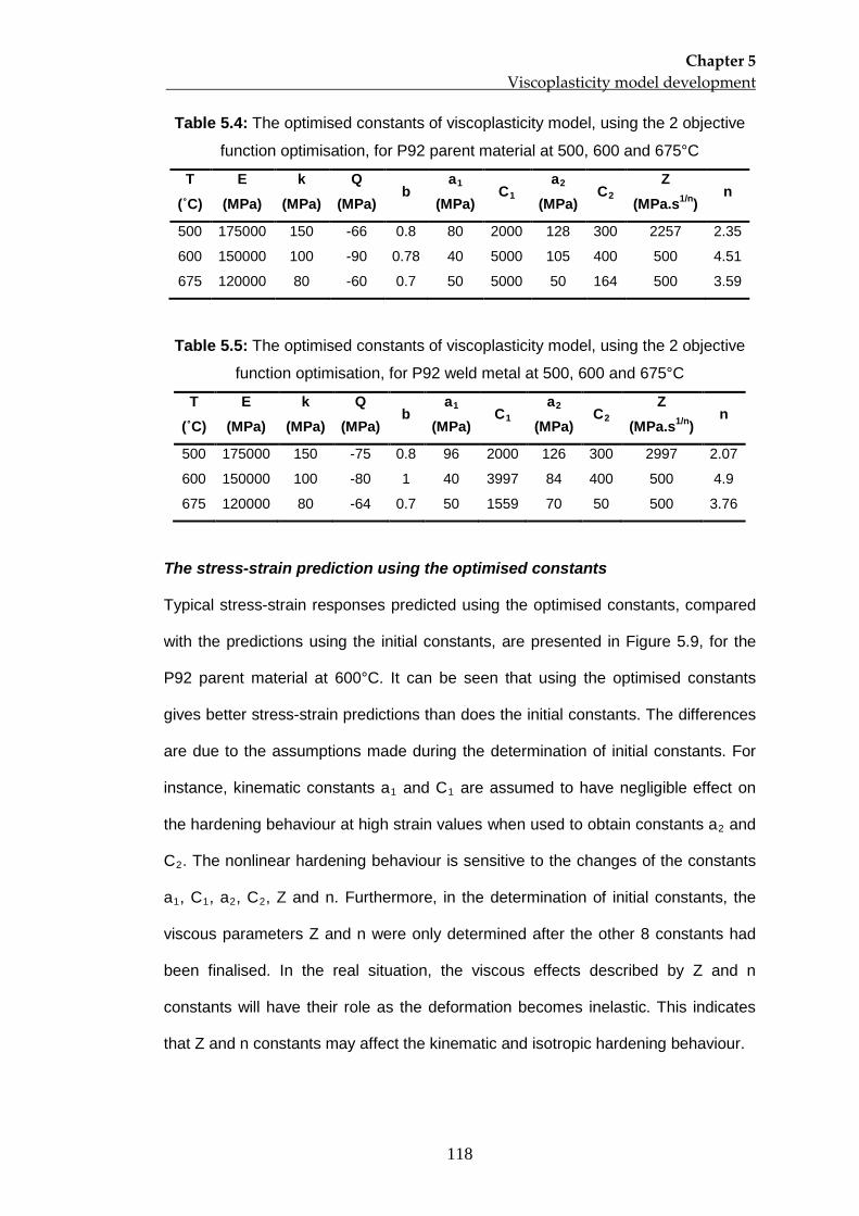
Chapter 5 Viscoplasticity model development
118
Table 5.4: The optimised constants of viscoplasticity model, using the 2 objective
function optimisation, for P92 parent material at 500, 600 and 675°C
T (˚C)
E (MPa)
k (MPa)
Q (MPa)
b a
(MPa) 1
Ca
1 (MPa)
2 C
Z 2
(MPa.s1/n n )
500 175000 150 -66 0.8 80 2000 128 300 2257 2.35
600 150000 100 -90 0.78 40 5000 105 400 500 4.51
675 120000 80 -60 0.7 50 5000 50 164 500 3.59
Table 5.5: The optimised constants of viscoplasticity model, using the 2 objective
function optimisation, for P92 weld metal at 500, 600 and 675°C
T (˚C)
E (MPa)
k (MPa)
Q (MPa)
b a
(MPa) 1
Ca
1 (MPa)
2 C
Z 2
(MPa.s1/n n )
500 175000 150 -75 0.8 96 2000 126 300 2997 2.07
600 150000 100 -80 1 40 3997 84 400 500 4.9
675 120000 80 -64 0.7 50 1559 70 50 500 3.76
The stress-strain prediction using the optimised constants
Typical stress-strain responses predicted using the optimised constants, compared
with the predictions using the initial constants, are presented in Figure 5.9, for the
P92 parent material at 600°C. It can be seen that using the optimised constants
gives better stress-strain predictions than does the initial constants. The differences
are due to the assumptions made during the determination of initial constants. For
instance, kinematic constants a1 and C1 are assumed to have negligible effect on
the hardening behaviour at high strain values when used to obtain constants a2 and
C2. The nonlinear hardening behaviour is sensitive to the changes of the constants
a1, C1, a2, C2
, Z and n. Furthermore, in the determination of initial constants, the
viscous parameters Z and n were only determined after the other 8 constants had
been finalised. In the real situation, the viscous effects described by Z and n
constants will have their role as the deformation becomes inelastic. This indicates
that Z and n constants may affect the kinematic and isotropic hardening behaviour.
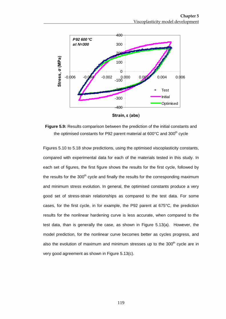
Chapter 5 Viscoplasticity model development
119
-400
-300
-200
-100
0
100
200
300
400
-0.006 -0.004 -0.002 0.000 0.002 0.004 0.006
Strain, ε (abs)
Stre
ss, σ
(MPa
)
Test
Initial
Optimised
P92 600 °Cat N=300
Figure 5.9: Results comparison between the prediction of the initial constants and
the optimised constants for P92 parent material at 600°C and 300th
cycle
Figures 5.10 to 5.18 show predictions, using the optimised viscoplasticity constants,
compared with experimental data for each of the materials tested in this study. In
each set of figures, the first figure shows the results for the first cycle, followed by
the results for the 300th cycle and finally the results for the corresponding maximum
and minimum stress evolution. In general, the optimised constants produce a very
good set of stress-strain relationships as compared to the test data. For some
cases, for the first cycle, in for example, the P92 parent at 675°C, the prediction
results for the nonlinear hardening curve is less accurate, when compared to the
test data, than is generally the case, as shown in Figure 5.13(a). However, the
model prediction, for the nonlinear curve becomes better as cycles progress, and
also the evolution of maximum and minimum stresses up to the 300th cycle are in
very good agreement as shown in Figure 5.13(c).
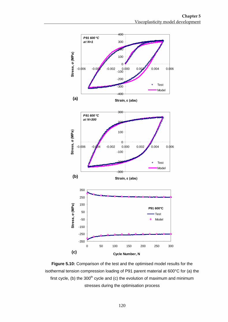
Chapter 5 Viscoplasticity model development
120
-400
-300
-200
-100
0
100
200
300
400
-0.006 -0.004 -0.002 0.000 0.002 0.004 0.006
Strain, ε (abs)
Stre
ss, σ
(MPa
)
Test
Model
P91 600 °Cat N=1
(a)
-300
-200
-100
0
100
200
300
-0.006 -0.004 -0.002 0.000 0.002 0.004 0.006
Strain, ε (abs)
Stre
ss, σ
(MPa
)
Test
Model
P91 600 °Cat N=300
(b)
-350
-250
-150
-50
50
150
250
350
0 50 100 150 200 250 300
Cycle Number, N
Stre
ss, σ
(MPa
)
Test
Model
P91 600°C
(c)
Figure 5.10: Comparison of the test and the optimised model results for the
isothermal tension compression loading of P91 parent material at 600°C for (a) the
first cycle, (b) the 300th cycle and (c) the evolution of maximum and minimum
stresses during the optimisation process
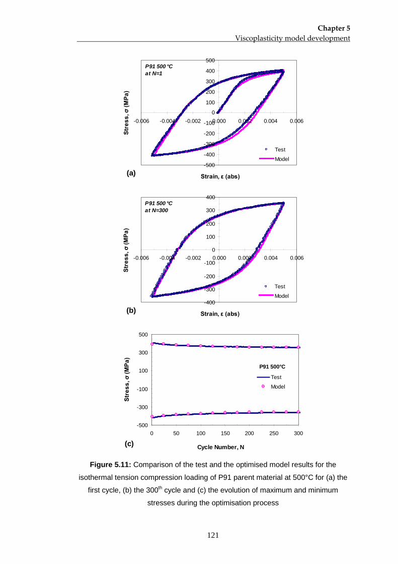
Chapter 5 Viscoplasticity model development
121
-500
-400
-300
-200
-100
0
100
200
300
400
500
-0.006 -0.004 -0.002 0.000 0.002 0.004 0.006
Strain, ε (abs)
Stre
ss, σ
(MPa
)
Test
Model
P91 500 °Cat N=1
(a)
-400
-300
-200
-100
0
100
200
300
400
-0.006 -0.004 -0.002 0.000 0.002 0.004 0.006
Strain, ε (abs)
Stre
ss, σ
(MPa
)
Test
Model
P91 500 °Cat N=300
(b)
-500
-300
-100
100
300
500
0 50 100 150 200 250 300
Cycle Number, N
Stre
ss, σ
(MPa
)
Test
Model
P91 500°C
(c)
Figure 5.11: Comparison of the test and the optimised model results for the
isothermal tension compression loading of P91 parent material at 500°C for (a) the
first cycle, (b) the 300th cycle and (c) the evolution of maximum and minimum
stresses during the optimisation process
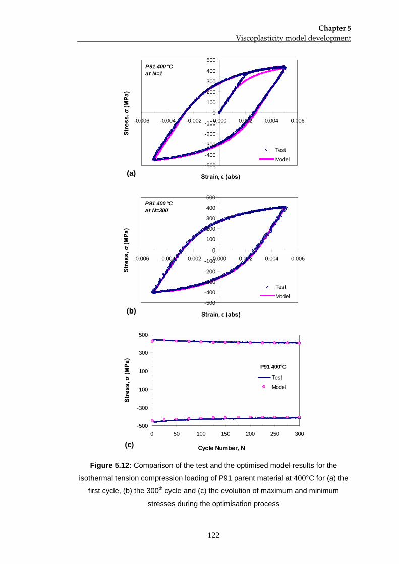
Chapter 5 Viscoplasticity model development
122
-500
-400
-300
-200
-100
0
100
200
300
400
500
-0.006 -0.004 -0.002 0.000 0.002 0.004 0.006
Strain, ε (abs)
Stre
ss, σ
(MPa
)
Test
Model
P91 400 °Cat N=1
(a)
-500
-400
-300
-200
-100
0
100
200
300
400
500
-0.006 -0.004 -0.002 0.000 0.002 0.004 0.006
Strain, ε (abs)
Stre
ss, σ
(MPa
)
Test
Model
P91 400 °Cat N=300
(b)
-500
-300
-100
100
300
500
0 50 100 150 200 250 300
Cycle Number, N
Stre
ss, σ
(MPa
)
Test
Model
P91 400°C
(c)
Figure 5.12: Comparison of the test and the optimised model results for the
isothermal tension compression loading of P91 parent material at 400°C for (a) the
first cycle, (b) the 300th cycle and (c) the evolution of maximum and minimum
stresses during the optimisation process
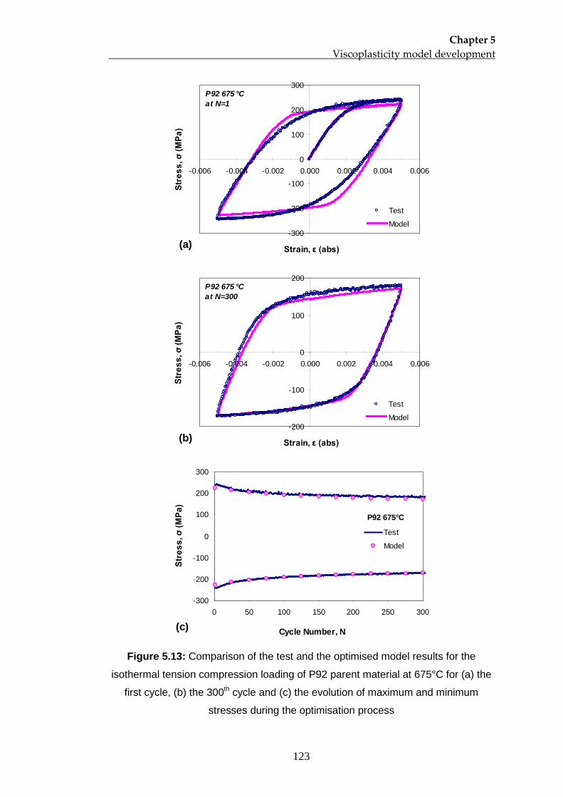
Chapter 5 Viscoplasticity model development
123
-300
-200
-100
0
100
200
300
-0.006 -0.004 -0.002 0.000 0.002 0.004 0.006
Strain, ε (abs)
Stre
ss, σ
(MPa
)
Test
Model
P92 675 °Cat N=1
(a)
-200
-100
0
100
200
-0.006 -0.004 -0.002 0.000 0.002 0.004 0.006
Strain, ε (abs)
Stre
ss, σ
(MPa
)
Test
Model
P92 675 °Cat N=300
(b)
-300
-200
-100
0
100
200
300
0 50 100 150 200 250 300
Cycle Number, N
Stre
ss, σ
(MPa
)
Test
Model
P92 675°C
(c)
Figure 5.13: Comparison of the test and the optimised model results for the
isothermal tension compression loading of P92 parent material at 675°C for (a) the
first cycle, (b) the 300th cycle and (c) the evolution of maximum and minimum
stresses during the optimisation process
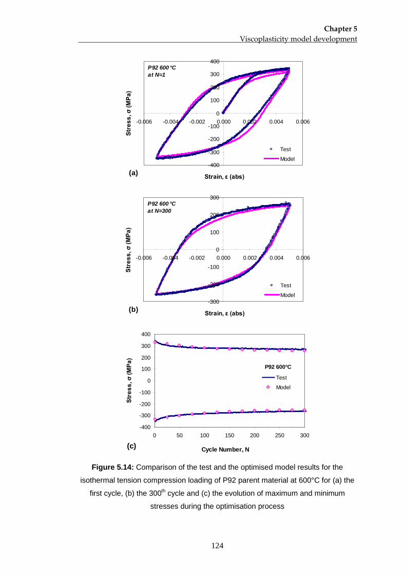
Chapter 5 Viscoplasticity model development
124
-400
-300
-200
-100
0
100
200
300
400
-0.006 -0.004 -0.002 0.000 0.002 0.004 0.006
Strain, ε (abs)
Stre
ss, σ
(MPa
)
Test
Model
P92 600 °Cat N=1
(a)
-300
-200
-100
0
100
200
300
-0.006 -0.004 -0.002 0.000 0.002 0.004 0.006
Strain, ε (abs)
Stre
ss, σ
(MPa
)
Test
Model
P92 600 °Cat N=300
(b)
-400
-300
-200
-100
0
100
200
300
400
0 50 100 150 200 250 300
Cycle Number, N
Stre
ss, σ
(MPa
)
Test
Model
P92 600°C
(c)
Figure 5.14: Comparison of the test and the optimised model results for the
isothermal tension compression loading of P92 parent material at 600°C for (a) the
first cycle, (b) the 300th
cycle and (c) the evolution of maximum and minimum
stresses during the optimisation process
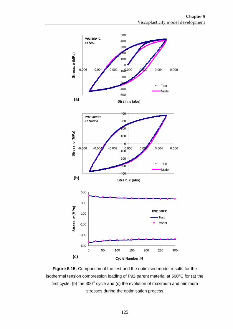
Chapter 5 Viscoplasticity model development
125
-500
-400
-300
-200
-100
0
100
200
300
400
500
-0.006 -0.004 -0.002 0.000 0.002 0.004 0.006
Strain, ε (abs)
Stre
ss, σ
(MPa
)
Test
Model
P92 500 °Cat N=1
(a)
-400
-300
-200
-100
0
100
200
300
400
-0.006 -0.004 -0.002 0.000 0.002 0.004 0.006
Strain, ε (abs)
Stre
ss, σ
(MPa
)
Test
Model
P92 500 °Cat N=300
(b)
-500
-300
-100
100
300
500
0 50 100 150 200 250 300
Cycle Number, N
Stre
ss, σ
(MPa
)
Test
Model
P92 500°C
(c)
Figure 5.15: Comparison of the test and the optimised model results for the
isothermal tension compression loading of P92 parent material at 500°C for (a) the
first cycle, (b) the 300th cycle and (c) the evolution of maximum and minimum
stresses during the optimisation process
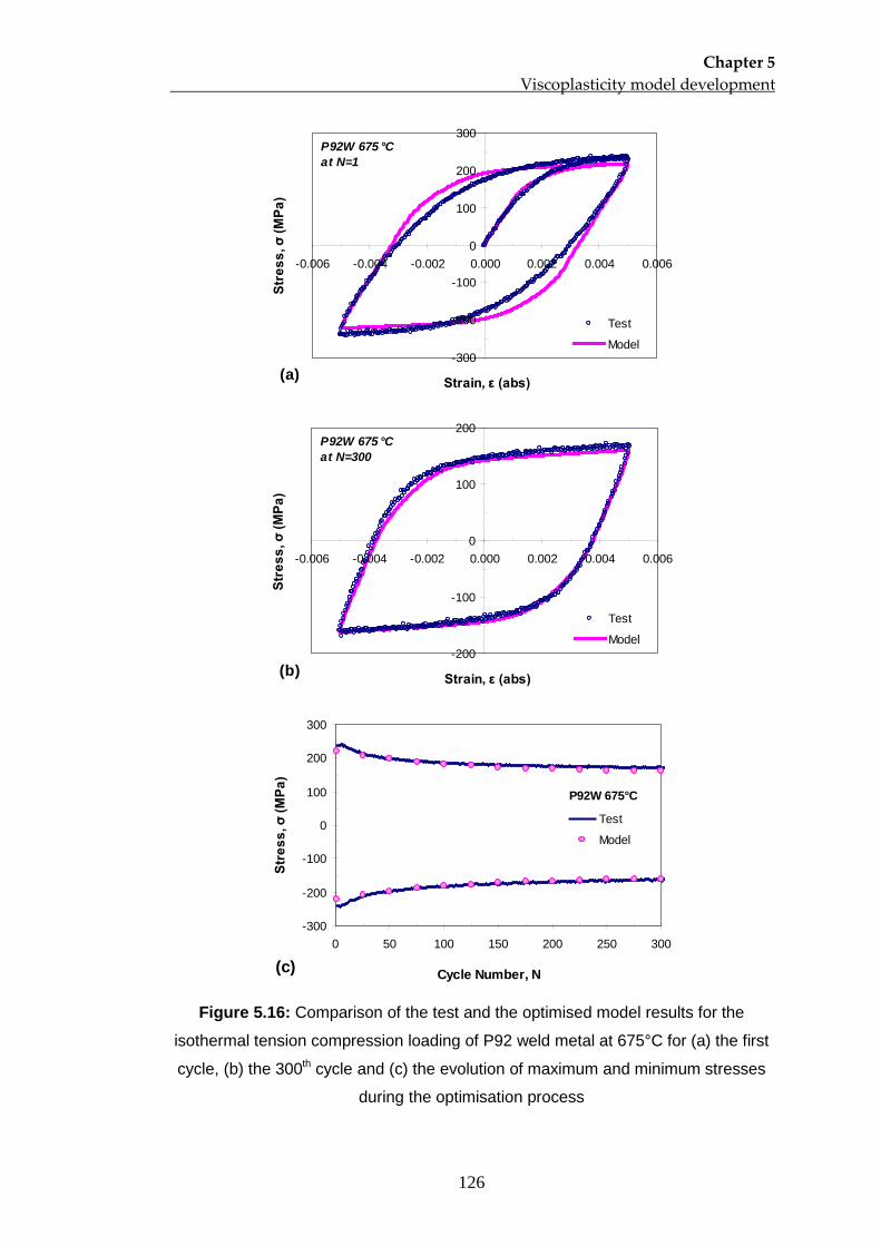
Chapter 5 Viscoplasticity model development
126
-300
-200
-100
0
100
200
300
-0.006 -0.004 -0.002 0.000 0.002 0.004 0.006
Strain, ε (abs)
Stre
ss, σ
(MPa
)
Test
Model
P92W 675 °Cat N=1
(a)
-200
-100
0
100
200
-0.006 -0.004 -0.002 0.000 0.002 0.004 0.006
Strain, ε (abs)
Stre
ss, σ
(MPa
)
Test
Model
P92W 675 °Cat N=300
(b)
-300
-200
-100
0
100
200
300
0 50 100 150 200 250 300
Cycle Number, N
Stre
ss, σ
(MPa
)
Test
Model
P92W 675°C
(c)
Figure 5.16: Comparison of the test and the optimised model results for the
isothermal tension compression loading of P92 weld metal at 675°C for (a) the first
cycle, (b) the 300th
cycle and (c) the evolution of maximum and minimum stresses
during the optimisation process
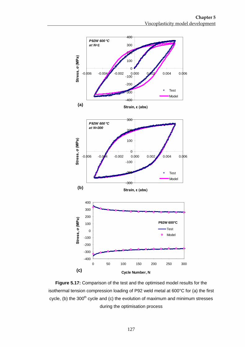
Chapter 5 Viscoplasticity model development
127
-400
-300
-200
-100
0
100
200
300
400
-0.006 -0.004 -0.002 0.000 0.002 0.004 0.006
Strain, ε (abs)
Stre
ss, σ
(MPa
)
Test
Model
P92W 600 °Cat N=1
(a)
-300
-200
-100
0
100
200
300
-0.006 -0.004 -0.002 0.000 0.002 0.004 0.006
Strain, ε (abs)
Stre
ss, σ
(MPa
)
Test
Model
P92W 600 °Cat N=300
(b)
-400
-300
-200
-100
0
100
200
300
400
0 50 100 150 200 250 300
Cycle Number, N
Stre
ss, σ
(MPa
)
Test
Model
P92W 600°C
(c)
Figure 5.17: Comparison of the test and the optimised model results for the
isothermal tension compression loading of P92 weld metal at 600°C for (a) the first
cycle, (b) the 300th
cycle and (c) the evolution of maximum and minimum stresses
during the optimisation process
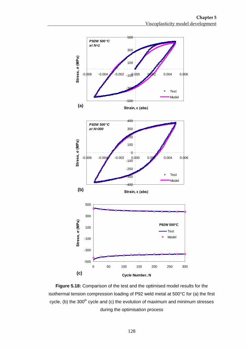
Chapter 5 Viscoplasticity model development
128
-500
-300
-100
100
300
500
-0.006 -0.004 -0.002 0.000 0.002 0.004 0.006
Strain, ε (abs)
Stre
ss, σ
(MPa
)
Test
Model
P92W 500 °Cat N=1
(a)
-400
-300
-200
-100
0
100
200
300
400
-0.006 -0.004 -0.002 0.000 0.002 0.004 0.006
Strain, ε (abs)
Stre
ss, σ
(MPa
)
Test
Model
P92W 500 °Cat N=300
(b)
-500
-300
-100
100
300
500
0 50 100 150 200 250 300
Cycle Number, N
Stre
ss, σ
(MPa
)
Test
Model
P92W 500°C
(c)
Figure 5.18: Comparison of the test and the optimised model results for the
isothermal tension compression loading of P92 weld metal at 500°C for (a) the first
cycle, (b) the 300th cycle and (c) the evolution of maximum and minimum stresses
during the optimisation process
Chapter 5 Viscoplasticity model development
129
5.4.2 Three objective function optimisation
The optimisation program in the previous section, which produced a set of
viscoplasticity constants with good predictions capability for the stress-strain
relationships, only focused on the tension-compression test data. However, the
effect of a constant dwell period was ignored in the program. From the results in the
section 3.6.2, it has been shown that the holding period for tensile strain at high
temperature in the isothermal strain-controlled tests produced a stress relaxation
behaviour in which the stress level drop in a constant strain controlled test. In this
section, a three objective function optimisation program has been used to improve
the performance of the viscoplasticity model. A similar optimisation program to that
program developed by Gong et al. (2010) was used for this purpose.
The three objective functions optimisation program considers three types of data in
the optimisation process. These are the stress-strain response, the evolution of
stress range which shows the cyclic softening behaviour and the stress relaxation
data during the holding period. An additional objective function equation was
defined as incorporated into equation (5.26) as follows:-
2exp3333 ))(()(
3
∑ −=M
ii
preixwxF σσ (5.30)
There are two limitations of the current 3 objective functions program. Firstly, the
program performs the optimisation process by considering only one supplied test
data, which is the test with a dwell period. The prediction of the resultant optimised
constants may give good prediction results if compared to the dwell test data only.
However, the set of determined constants may give less accurate prediction of the
tension-compression data, particularly at higher number of cycles. This kind of
situation was observed in the initial stage of using the three objective functions
Chapter 5 Viscoplasticity model development
130
program. Secondly, the optimisation can only be done using a limited number of
cycles, for example only experimental data within 20 cycles were used in this study.
The current 3 objective functions program is still being improved in order to include
more data during the optimisation process.
In order to produce a set of constants which satisfy both sets of test data, several
procedures were implemented. At the end of the optimisation process using the
three-objective function program, the optimised constants performance compared to
the tension-compression data were performed manually. If the results were not in a
good agreement, the optimisation process using the three objective functions was
repeated by changing the boundaries of the lower and upper constants in the
program. The optimisation process may need to be repeated several times, with the
help of spreadsheet calculation to select the constant boundaries, in order to obtain
a set of constants which gives reasonably good predictions for both types of test
data. The optimised constants obtained using the 3 objective function program are
given in Table 5.6, 5.7 and 5.8 for the P91 parent material, P92 parent material and
P92 weld metal, respectively. Due to limitation of P92 material, only two isothermal
tensile peak strain dwell tests were performed which are at 600 and 675°C. So, the
optimisation using the 3 objective function program at 500°C cannot be
implemented.
Some of the predictions of the optimised constants in this section are shown in
Figures 5.19 to 5.22. Figure 5.19(a) shows the effect of the three-objective functions
program on the prediction of stress relaxation behaviour in which a better shape and
better stress values are achieved. Although the optimisation was implemented using
data from 20 cycles, the determined set of constants give reasonable predictions at
higher cycles than 20, as shown in Figure 5.19(b). As mentioned earlier, a repeated
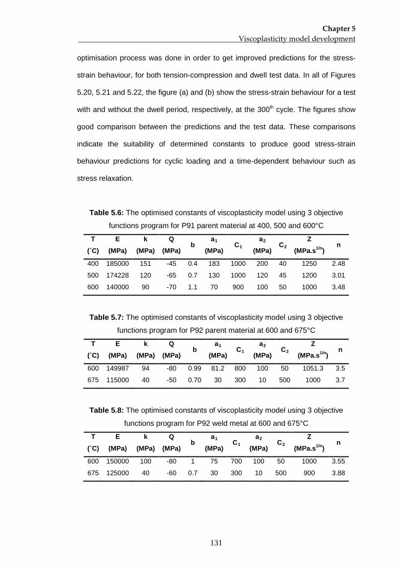
Chapter 5 Viscoplasticity model development
131
optimisation process was done in order to get improved predictions for the stress-
strain behaviour, for both tension-compression and dwell test data. In all of Figures
5.20, 5.21 and 5.22, the figure (a) and (b) show the stress-strain behaviour for a test
with and without the dwell period, respectively, at the 300th
cycle. The figures show
good comparison between the predictions and the test data. These comparisons
indicate the suitability of determined constants to produce good stress-strain
behaviour predictions for cyclic loading and a time-dependent behaviour such as
stress relaxation.
Table 5.6: The optimised constants of viscoplasticity model using 3 objective
functions program for P91 parent material at 400, 500 and 600°C
T (˚C)
E (MPa)
k (MPa)
Q (MPa)
b a
(MPa) 1
Ca
1 (MPa)
2 C
Z 2
(MPa.s1/n n )
400 185000 151 -45 0.4 183 1000 200 40 1250 2.48
500 174228 120 -65 0.7 130 1000 120 45 1200 3.01
600 140000 90 -70 1.1 70 900 100 50 1000 3.48
Table 5.7: The optimised constants of viscoplasticity model using 3 objective
functions program for P92 parent material at 600 and 675°C
T (˚C)
E (MPa)
k (MPa)
Q (MPa)
b a
(MPa) 1
Ca
1 (MPa)
2 C
Z 2
(MPa.s1/n n )
600 149987 94 -80 0.99 81.2 800 100 50 1051.3 3.5
675 115000 40 -50 0.70 30 300 10 500 1000 3.7
Table 5.8: The optimised constants of viscoplasticity model using 3 objective
functions program for P92 weld metal at 600 and 675°C
T (˚C)
E (MPa)
k (MPa)
Q (MPa)
b a
(MPa) 1
Ca
1 (MPa)
2 C
Z 2
(MPa.s1/n n )
600 150000 100 -80 1 75 700 100 50 1000 3.55
675 125000 40 -60 0.7 30 300 10 500 900 3.88
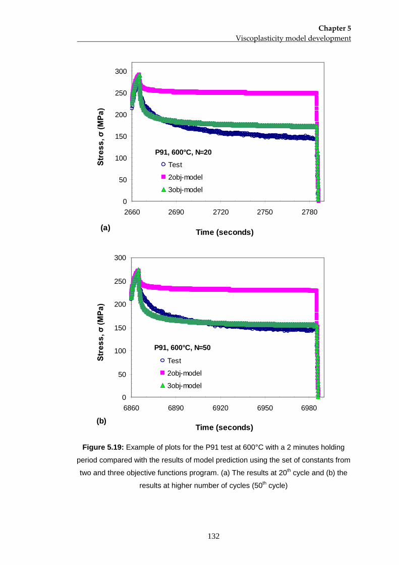
Chapter 5 Viscoplasticity model development
132
0
50
100
150
200
250
300
2660 2690 2720 2750 2780
Time (seconds)
Stre
ss, σ
(MPa
)
Test
2obj-model
3obj-model
P91, 600°C, N=20
(a)
0
50
100
150
200
250
300
6860 6890 6920 6950 6980
Time (seconds)
Stre
ss, σ
(MPa
)
Test
2obj-model
3obj-model
P91, 600°C, N=50
(b)
Figure 5.19: Example of plots for the P91 test at 600°C with a 2 minutes holding
period compared with the results of model prediction using the set of constants from
two and three objective functions program. (a) The results at 20th cycle and (b) the
results at higher number of cycles (50th
cycle)
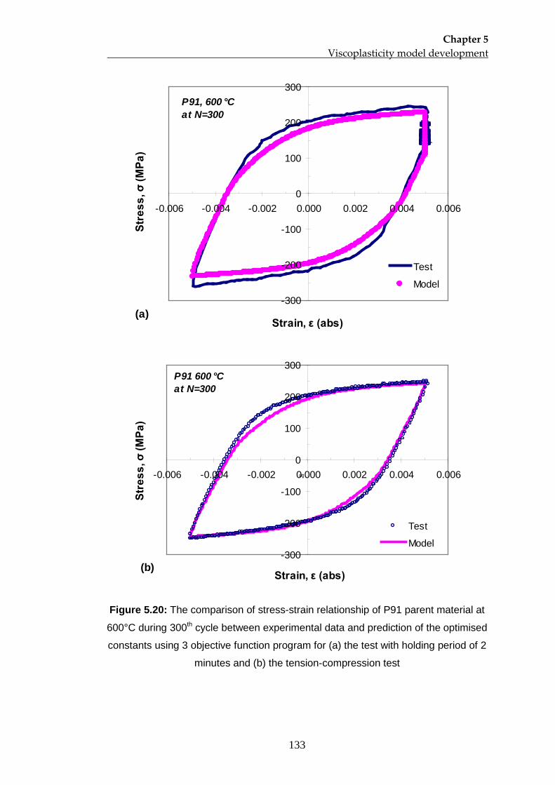
Chapter 5 Viscoplasticity model development
133
-300
-200
-100
0
100
200
300
-0.006 -0.004 -0.002 0.000 0.002 0.004 0.006
Strain, ε (abs)
Stre
ss, σ
(MPa
)
Test
Model
P91, 600 °Cat N=300
(a)
-300
-200
-100
0
100
200
300
-0.006 -0.004 -0.002 0.000 0.002 0.004 0.006
Strain, ε (abs)
Stre
ss, σ
(MPa
)
Test
Model
P91 600 °Cat N=300
(b)
un
Figure 5.20: The comparison of stress-strain relationship of P91 parent material at
600°C during 300th
cycle between experimental data and prediction of the optimised
constants using 3 objective function program for (a) the test with holding period of 2
minutes and (b) the tension-compression test
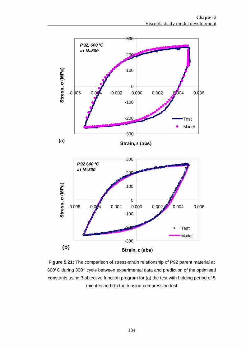
Chapter 5 Viscoplasticity model development
134
-300
-200
-100
0
100
200
300
-0.006 -0.004 -0.002 0.000 0.002 0.004 0.006
Strain, ε (abs)
Stre
ss, σ
(MPa
)
Test
Model
P92, 600 °Cat N=300
(a)
-300
-200
-100
0
100
200
300
-0.006 -0.004 -0.002 0.000 0.002 0.004 0.006
Strain, ε (abs)
Stre
ss, σ
(MPa
)
Test
Model
P92 600 °Cat N=300
(b)
Figure 5.21: The comparison of stress-strain relationship of P92 parent material at
600°C during 300th
cycle between experimental data and prediction of the optimised
constants using 3 objective function program for (a) the test with holding period of 5
minutes and (b) the tension-compression test
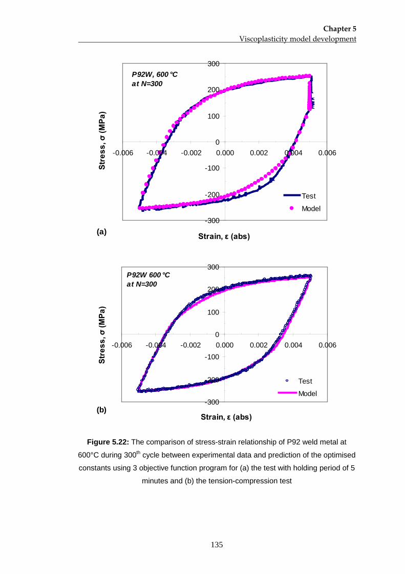
Chapter 5 Viscoplasticity model development
135
-300
-200
-100
0
100
200
300
-0.006 -0.004 -0.002 0.000 0.002 0.004 0.006
Strain, ε (abs)
Stre
ss, σ
(MPa
)
Test
Model
P92W, 600 °Cat N=300
(a)
-300
-200
-100
0
100
200
300
-0.006 -0.004 -0.002 0.000 0.002 0.004 0.006
Strain, ε (abs)
Stre
ss, σ
(MPa
)
Test
Model
P92W 600 °Cat N=300
(b)
Figure 5.22: The comparison of stress-strain relationship of P92 weld metal at
600°C during 300th
cycle between experimental data and prediction of the optimised
constants using 3 objective function program for (a) the test with holding period of 5
minutes and (b) the tension-compression test
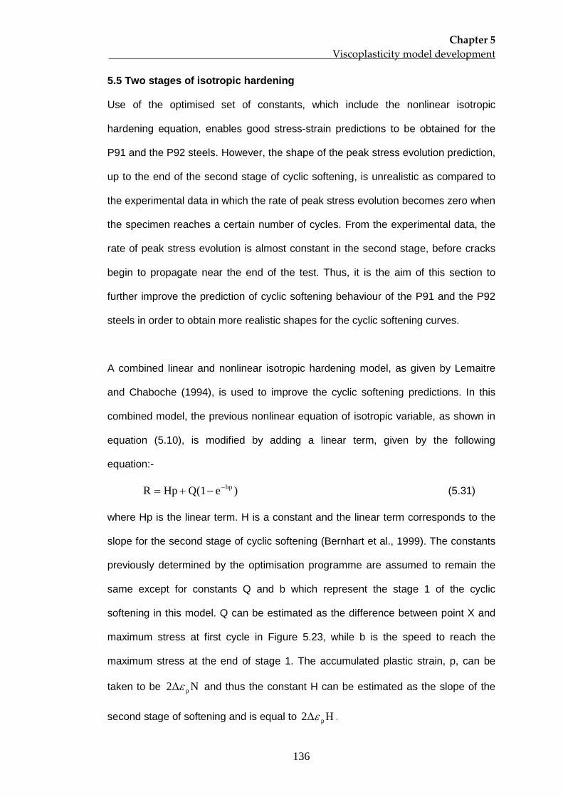
Chapter 5 Viscoplasticity model development
136
5.5 Two stages of isotropic hardening
Use of the optimised set of constants, which include the nonlinear isotropic
hardening equation, enables good stress-strain predictions to be obtained for the
P91 and the P92 steels. However, the shape of the peak stress evolution prediction,
up to the end of the second stage of cyclic softening, is unrealistic as compared to
the experimental data in which the rate of peak stress evolution becomes zero when
the specimen reaches a certain number of cycles. From the experimental data, the
rate of peak stress evolution is almost constant in the second stage, before cracks
begin to propagate near the end of the test. Thus, it is the aim of this section to
further improve the prediction of cyclic softening behaviour of the P91 and the P92
steels in order to obtain more realistic shapes for the cyclic softening curves.
A combined linear and nonlinear isotropic hardening model, as given by Lemaitre
and Chaboche (1994), is used to improve the cyclic softening predictions. In this
combined model, the previous nonlinear equation of isotropic variable, as shown in
equation (5.10), is modified by adding a linear term, given by the following
equation:-
)eQ(1HpR bp−−+= (5.31)
where Hp is the linear term. H is a constant and the linear term corresponds to the
slope for the second stage of cyclic softening (Bernhart et al., 1999). The constants
previously determined by the optimisation programme are assumed to remain the
same except for constants Q and b which represent the stage 1 of the cyclic
softening in this model. Q can be estimated as the difference between point X and
maximum stress at first cycle in Figure 5.23, while b is the speed to reach the
maximum stress at the end of stage 1. The accumulated plastic strain, p, can be
taken to be N2Δ pε and thus the constant H can be estimated as the slope of the
second stage of softening and is equal to H2Δ pε .
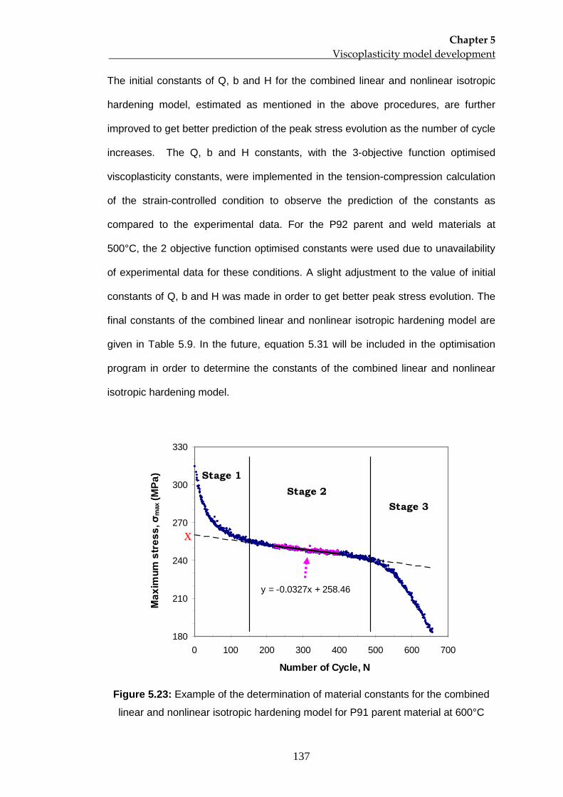
Chapter 5 Viscoplasticity model development
137
The initial constants of Q, b and H for the combined linear and nonlinear isotropic
hardening model, estimated as mentioned in the above procedures, are further
improved to get better prediction of the peak stress evolution as the number of cycle
increases. The Q, b and H constants, with the 3-objective function optimised
viscoplasticity constants, were implemented in the tension-compression calculation
of the strain-controlled condition to observe the prediction of the constants as
compared to the experimental data. For the P92 parent and weld materials at
500°C, the 2 objective function optimised constants were used due to unavailability
of experimental data for these conditions. A slight adjustment to the value of initial
constants of Q, b and H was made in order to get better peak stress evolution. The
final constants of the combined linear and nonlinear isotropic hardening model are
given in Table 5.9. In the future, equation 5.31 will be included in the optimisation
program in order to determine the constants of the combined linear and nonlinear
isotropic hardening model.
y = -0.0327x + 258.46
180
210
240
270
300
330
0 100 200 300 400 500 600 700
Number of Cycle, N
Max
imum
str
ess,
σm
ax (M
Pa) Stage 1
Stage 2Stage 3
X
Figure 5.23: Example of the determination of material constants for the combined
linear and nonlinear isotropic hardening model for P91 parent material at 600°C
Chapter 5 Viscoplasticity model development
138
Table 5.9: The material constants of the combined linear and nonlinear isotropic
hardening model for P91 parent, P92 parent and P92 weld metal at different
temperatures
Constants P91 parent P92 parent P92 weld
400°C 500°C 600°C 500°C 600°C 675°C 500°C 600°C 675°C
Q -30 -42 -52 -52 -58 -40 -55 -60 -45
b 0.8 1.3 1.9 1.1 1.6 1.2 1.2 1.3 1.2
H -1.8 -2.1 -2.9 -2.7 -2.7 -1.6 -3.5 -2.7 -1.9
Figure 5.24 shows the predictions obtained using the viscoplasticity model for P91
parent material at 600°C using the nonlinear equation and the combined linear-
nonlinear equation for isotropic hardening model. It can be seen in the figure that
the peak stress level prediction using the nonlinear isotropic hardening model
becomes constant around 300th cycles onwards. Also, a clear gap exists between
the test data and the model predictions, using the nonlinear model, located at
around 200th cycles, even though the maximum stress difference at the 200th cycle
is only around 6 MPa. It is clear that the isotropic hardening model with the
combined linear-nonlinear model has improved the prediction of the peak stresses
evolution shape, as shown in Figure 5.24, which is more realistic to represent the
linear curve of the cyclic softening in the secondary stage. The prediction of the
cyclic softening shape is good up to the end of secondary stage before the final
stage of rapid softening occurs due to crack propagation in the material. The current
model is unable to predict the final stage of cyclic softening unless a damage
mechanics concept is introduced into the model, which is the subject of another
research program. The predictions of the stress evolution for each specimen at
different temperatures, using the linear nonlinear isotropic hardening model
constants in Table 5.9, are shown in Figures 5.25, 5.26 and 5.27 for the P91 parent,
P92 parent and P92 weld metal respectively. All of the predictions are in good
agreement with the experimental data.
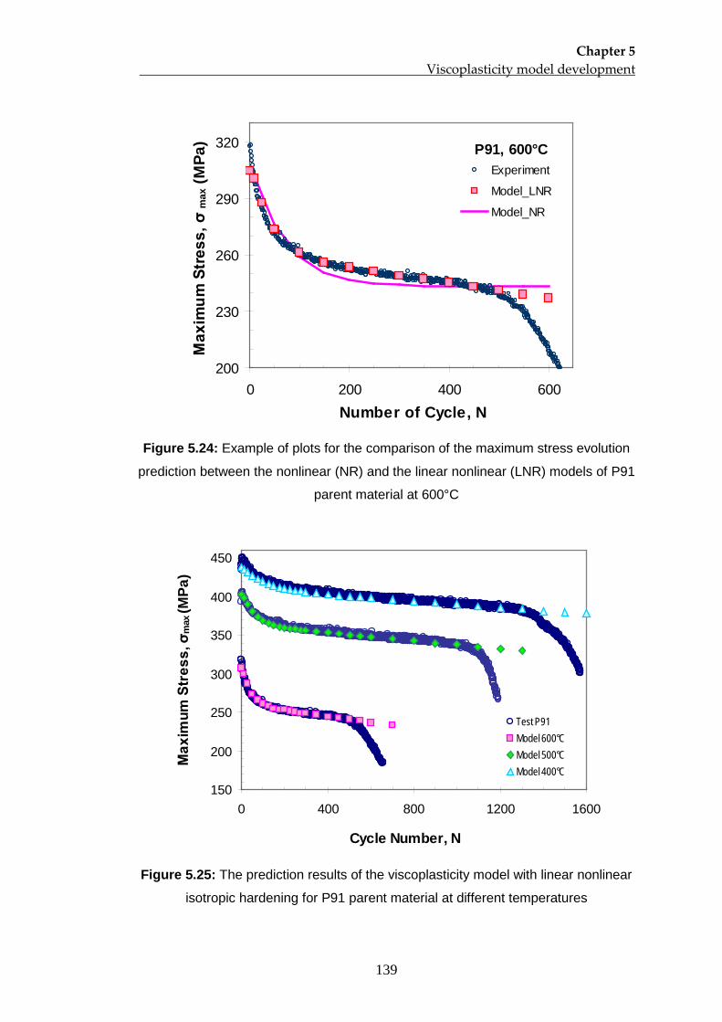
Chapter 5 Viscoplasticity model development
139
200
230
260
290
320
0 200 400 600Number of Cycle, N
Max
imum
Str
ess,
σm
ax (M
Pa)
Experiment
Model_LNR
Model_NR
P91, 600°C
Figure 5.24: Example of plots for the comparison of the maximum stress evolution
prediction between the nonlinear (NR) and the linear nonlinear (LNR) models of P91
parent material at 600°C
150
200
250
300
350
400
450
0 400 800 1200 1600
Cycle Number, N
Max
imum
Str
ess,
σm
ax (M
Pa)
Test P91Model 600°CModel 500°CModel 400°C
Figure 5.25: The prediction results of the viscoplasticity model with linear nonlinear
isotropic hardening for P91 parent material at different temperatures
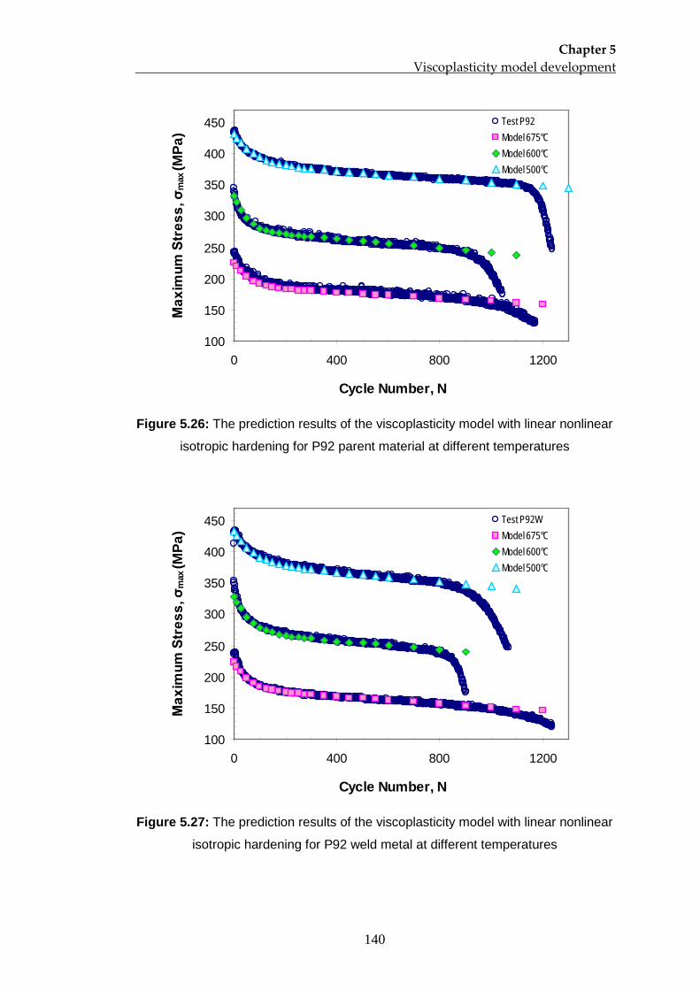
Chapter 5 Viscoplasticity model development
140
100
150
200
250
300
350
400
450
0 400 800 1200
Cycle Number, N
Max
imum
Str
ess,
σm
ax (M
Pa)
Test P92Model 675°CModel 600°CModel 500°C
Figure 5.26: The prediction results of the viscoplasticity model with linear nonlinear
isotropic hardening for P92 parent material at different temperatures
100
150
200
250
300
350
400
450
0 400 800 1200
Cycle Number, N
Max
imum
Str
ess,
σm
ax (M
Pa)
Test P92WModel 675°CModel 600°CModel 500°C
Figure 5.27: The prediction results of the viscoplasticity model with linear nonlinear
isotropic hardening for P92 weld metal at different temperatures
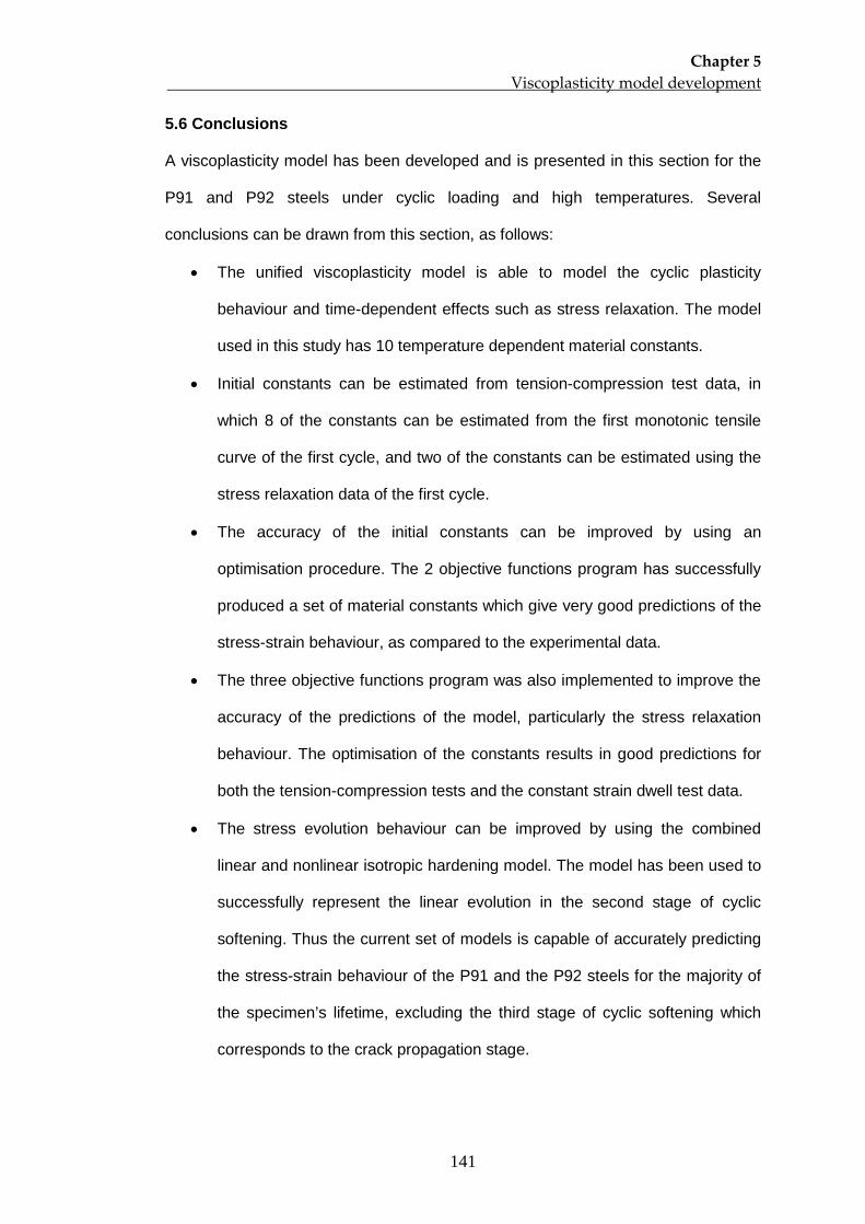
Chapter 5 Viscoplasticity model development
141
5.6 Conclusions
A viscoplasticity model has been developed and is presented in this section for the
P91 and P92 steels under cyclic loading and high temperatures. Several
conclusions can be drawn from this section, as follows:
• The unified viscoplasticity model is able to model the cyclic plasticity
behaviour and time-dependent effects such as stress relaxation. The model
used in this study has 10 temperature dependent material constants.
• Initial constants can be estimated from tension-compression test data, in
which 8 of the constants can be estimated from the first monotonic tensile
curve of the first cycle, and two of the constants can be estimated using the
stress relaxation data of the first cycle.
• The accuracy of the initial constants can be improved by using an
optimisation procedure. The 2 objective functions program has successfully
produced a set of material constants which give very good predictions of the
stress-strain behaviour, as compared to the experimental data.
• The three objective functions program was also implemented to improve the
accuracy of the predictions of the model, particularly the stress relaxation
behaviour. The optimisation of the constants results in good predictions for
both the tension-compression tests and the constant strain dwell test data.
• The stress evolution behaviour can be improved by using the combined
linear and nonlinear isotropic hardening model. The model has been used to
successfully represent the linear evolution in the second stage of cyclic
softening. Thus the current set of models is capable of accurately predicting
the stress-strain behaviour of the P91 and the P92 steels for the majority of
the specimen’s lifetime, excluding the third stage of cyclic softening which
corresponds to the crack propagation stage.
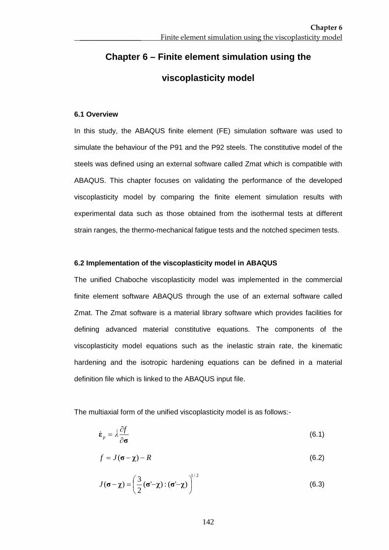
Chapter 6 _________________ Finite element simulation using the viscoplasticity model
142
Chapter 6 – Finite element simulation using the
viscoplasticity model
6.1 Overview
In this study, the ABAQUS finite element (FE) simulation software was used to
simulate the behaviour of the P91 and the P92 steels. The constitutive model of the
steels was defined using an external software called Zmat which is compatible with
ABAQUS. This chapter focuses on validating the performance of the developed
viscoplasticity model by comparing the finite element simulation results with
experimental data such as those obtained from the isothermal tests at different
strain ranges, the thermo-mechanical fatigue tests and the notched specimen tests.
6.2 Implementation of the viscoplasticity model in ABAQUS
The unified Chaboche viscoplasticity model was implemented in the commercial
finite element software ABAQUS through the use of an external software called
Zmat. The Zmat software is a material library software which provides facilities for
defining advanced material constitutive equations. The components of the
viscoplasticity model equations such as the inelastic strain rate, the kinematic
hardening and the isotropic hardening equations can be defined in a material
definition file which is linked to the ABAQUS input file.
The multiaxial form of the unified viscoplasticity model is as follows:-
σ
ε∂∂
=fλp
(6.1)
RJf −−= )( χσ (6.2)
2/1
)'(:)'(23)(
−−=− χσχσχσJ (6.3)
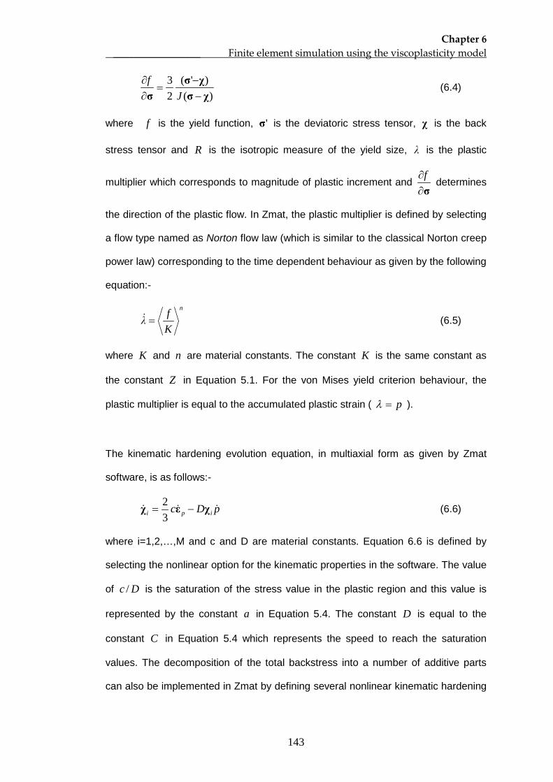
Chapter 6 _________________ Finite element simulation using the viscoplasticity model
143
)(
)'(23
χσχσ
σ −−
=∂∂
Jf
(6.4)
where f is the yield function, 'σ is the deviatoric stress tensor, χ is the back
stress tensor and R is the isotropic measure of the yield size, λ is the plastic
multiplier which corresponds to magnitude of plastic increment and σ∂∂f
determines
the direction of the plastic flow. In Zmat, the plastic multiplier is defined by selecting
a flow type named as Norton flow law (which is similar to the classical Norton creep
power law) corresponding to the time dependent behaviour as given by the following
equation:-
n
Kfλ = (6.5)
where K and n are material constants. The constant K is the same constant as
the constant Z in Equation 5.1. For the von Mises yield criterion behaviour, the
plastic multiplier is equal to the accumulated plastic strain ( p=λ ).
The kinematic hardening evolution equation, in multiaxial form as given by Zmat
software, is as follows:-
pDc ipi χεχ −=32
(6.6)
where i=1,2,…,M and c and D are material constants. Equation 6.6 is defined by
selecting the nonlinear option for the kinematic properties in the software. The value
of Dc / is the saturation of the stress value in the plastic region and this value is
represented by the constant a in Equation 5.4. The constant D is equal to the
constant C in Equation 5.4 which represents the speed to reach the saturation
values. The decomposition of the total backstress into a number of additive parts
can also be implemented in Zmat by defining several nonlinear kinematic hardening
Chapter 6 _________________ Finite element simulation using the viscoplasticity model
144
properties in the material definition file. In this study, it has been chosen that M=2 in
order to decompose the kinematic hardening equations into two components.
The isotropic hardening equation, as given in Equation 5.10, is defined in Zmat by
selecting the nonlinear option for the isotropic properties and the nonlinear isotropic
hardening in Zmat is given by the following equation:-
)1(0bpeQRR −−+= (6.7)
where constant Q is the asymptotic value of the isotropic variable, constant b is
related to the speed towards saturation and the saturation yield surface radius will
be QR +0 for large accumulated plastic strain. The value of 0R for initial yield
surface radius is noted here to be the onset of plasticity, and not the engineering
yield stress, and the method of determining this constant is explained in section
5.3.1. As the P91 and the P92 steels exhibit a gradual linear decrease in the middle
of the test period, after a nonlinear decrease of stress amplitudes, the isotropic
hardening behaviour is better described by the two-stage isotropic hardening model,
as described in Chapter 5 as the combined linear and nonlinear isotropic hardening.
In Zmat, the “linear_nonlinear” option can be selected for this purpose and its
equation is given as follows:-
)1(0bpeQHpRR −−++= (6.8)
where H is a material constant representing the slope of the linear period during
cyclic softening of the steels. The examples of the Zmat’s material definition file for
the unified viscoplasticity model are given in the appendix section.
6.3 FE simulation of the isothermal cyclic loading
The optimized viscoplasticity constants for the P91 and P92 steels in this study
were determined using the isothermal strain-controlled test data with a ±0.5% strain
amplitude at different temperatures. In this section, the optimised viscoplasticity
Chapter 6 _________________ Finite element simulation using the viscoplasticity model
145
model with linear nonlinear isotropic hardening at 600°C was used in finite element
simulation in order to simulate the isothermal stress-strain behaviour at different
strain ranges, namely ±0.2%, ±0.25% and 0.4% strain amplitudes and to compare
the simulation results with the experimental data. The cyclic period for each
simulation was identical to its testing period with a 0.1%/s strain rate.
An axisymmetric model with a 3.25mm radius, R1, and a 7.5mm height, H, as
shown in Figure 6.1(a), was used in the simulation to represent the gauge section of
the solid specimen, where the extensometer arms were placed during the strain-
controlled tests. Figure 6.1(b) shows the axisymmetric model of the tubular
specimen, with a 2mm inner radius, R2
, used for the thermomechanical fatigue
tests. Displacement control was applied in order to obtain the same strain range as
that for the experimental data. The boundary conditions on the axisymmetric models
are shown in Figures 6.1(a) and 6.1(b). The 8-node biquadratic, reduced
integration, element, called CAX8R in the Abaqus finite element software, were
used for all the geometries presented in this chapter.
Figures 6.2 to 6.4 show the comparison between the simulation and the testing
results of the P91 steels performed at 600°C with ±0.4%, ±0.25% and ±0.2% strain
amplitudes, respectively. The simulation and the testing results show good
comparison at each test particularly at the first complete cycle. The stress amplitude
recorded in each cycle decreases as the number of cycle increases and a larger
number of cycles is required to achieve the saturation period of the cyclic softening
for the tests with lower strain amplitudes. The comparison of these results with
experimental data shows promising results up to the secondary stage of cyclic
softening for each test with different strain amplitudes. The results in this section
indicate the suitability of selecting the strain-controlled test data with higher strain
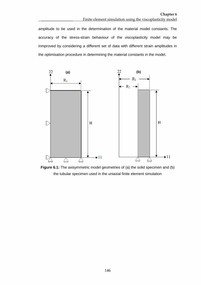
Chapter 6 _________________ Finite element simulation using the viscoplasticity model
146
amplitude to be used in the determination of the material model constants. The
accuracy of the stress-strain behaviour of the viscoplasticity model may be
inmproved by considering a different set of data with different strain amplitudes in
the optimisation procedure in determining the material constants in the model.
Figure 6.1: The axisymmetric model geometries of (a) the solid specimen and (b)
the tubular specimen used in the uniaxial finite element simulation
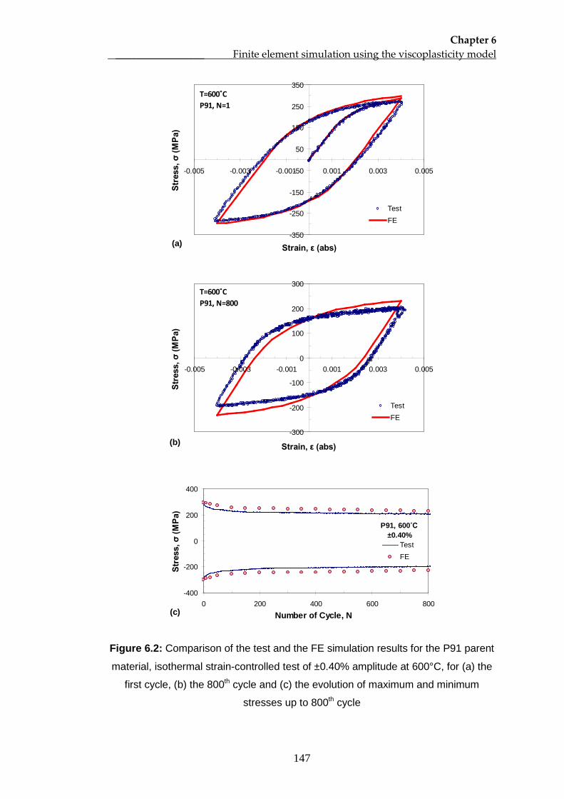
Chapter 6 _________________ Finite element simulation using the viscoplasticity model
147
-350
-250
-150
-50
50
150
250
350
-0.005 -0.003 -0.001 0.001 0.003 0.005
Strain, ε (abs)
Stre
ss, σ
(MPa
)
TestFE
T=600˚CP91, N=1
(a)
-300
-200
-100
0
100
200
300
-0.005 -0.003 -0.001 0.001 0.003 0.005
Strain, ε (abs)
Stre
ss, σ
(MPa
)
TestFE
T=600˚CP91, N=800
(b)
-400
-200
0
200
400
0 200 400 600 800Number of Cycle, N
Stre
ss, σ
(MPa
)
TestFE
P91, 600˚C ±0.40%
(c)
Figure 6.2: Comparison of the test and the FE simulation results for the P91 parent
material, isothermal strain-controlled test of ±0.40% amplitude at 600°C, for (a) the
first cycle, (b) the 800th cycle and (c) the evolution of maximum and minimum
stresses up to 800th
cycle
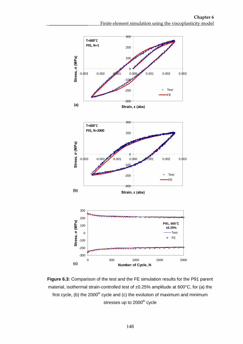
Chapter 6 _________________ Finite element simulation using the viscoplasticity model
148
-300
-200
-100
0
100
200
300
-0.003 -0.002 -0.001 0.000 0.001 0.002 0.003
Strain, ε (abs)
Stre
ss, σ
(MPa
)
TestFE
T=600˚CP91, N=1
(a)
-300
-200
-100
0
100
200
300
-0.003 -0.002 -0.001 0.000 0.001 0.002 0.003
Strain, ε (abs)
Stre
ss, σ
(MPa
)
TestFE
T=600˚CP91, N=2000
(b)
-300
-200
-100
0
100
200
300
0 500 1000 1500 2000Number of Cycle, N
Stre
ss, σ
(MPa
)
TestFE
P91, 600˚C ±0.25%
(c)
Figure 6.3: Comparison of the test and the FE simulation results for the P91 parent
material, isothermal strain-controlled test of ±0.25% amplitude at 600°C, for (a) the
first cycle, (b) the 2000th cycle and (c) the evolution of maximum and minimum
stresses up to 2000th
cycle
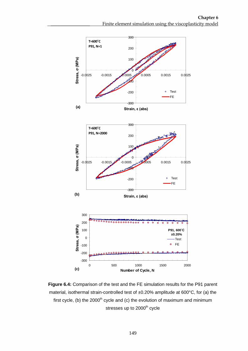
Chapter 6 _________________ Finite element simulation using the viscoplasticity model
149
-300
-200
-100
0
100
200
300
-0.0025 -0.0015 -0.0005 0.0005 0.0015 0.0025
Strain, ε (abs)
Stre
ss, σ
(MPa
)
TestFE
T=600˚CP91, N=1
(a)
-300
-200
-100
0
100
200
300
-0.0025 -0.0015 -0.0005 0.0005 0.0015 0.0025
Strain, ε (abs)
Stre
ss, σ
(MPa
)
TestFE
T=600˚CP91, N=2000
(b)
-300
-200
-100
0
100
200
300
0 500 1000 1500 2000Number of Cycle, N
Stre
ss, σ
(MPa
)
TestFE
P91, 600˚C ±0.20%
(c)
Figure 6.4: Comparison of the test and the FE simulation results for the P91 parent
material, isothermal strain-controlled test of ±0.20% amplitude at 600°C, for (a) the
first cycle, (b) the 2000th cycle and (c) the evolution of maximum and minimum
stresses up to 2000th
cycle
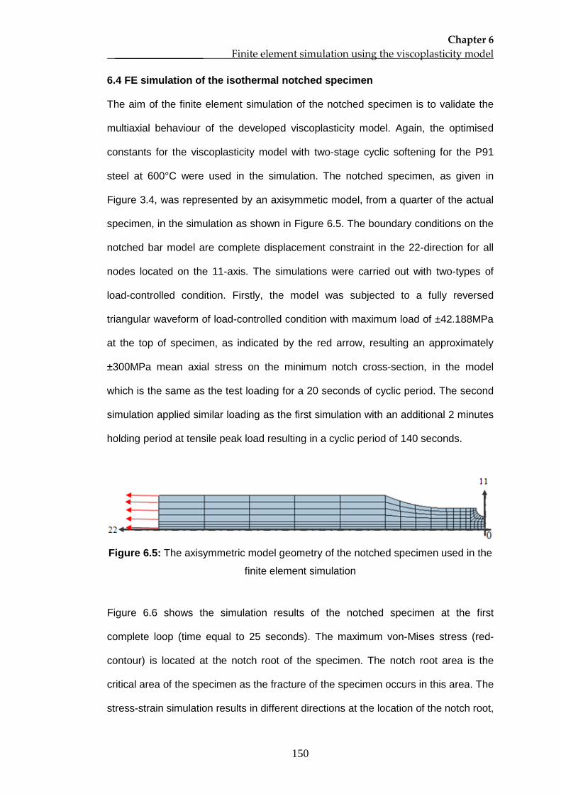
Chapter 6 _________________ Finite element simulation using the viscoplasticity model
150
6.4 FE simulation of the isothermal notched specimen
The aim of the finite element simulation of the notched specimen is to validate the
multiaxial behaviour of the developed viscoplasticity model. Again, the optimised
constants for the viscoplasticity model with two-stage cyclic softening for the P91
steel at 600°C were used in the simulation. The notched specimen, as given in
Figure 3.4, was represented by an axisymmetic model, from a quarter of the actual
specimen, in the simulation as shown in Figure 6.5. The boundary conditions on the
notched bar model are complete displacement constraint in the 22-direction for all
nodes located on the 11-axis. The simulations were carried out with two-types of
load-controlled condition. Firstly, the model was subjected to a fully reversed
triangular waveform of load-controlled condition with maximum load of ±42.188MPa
at the top of specimen, as indicated by the red arrow, resulting an approximately
±300MPa mean axial stress on the minimum notch cross-section, in the model
which is the same as the test loading for a 20 seconds of cyclic period. The second
simulation applied similar loading as the first simulation with an additional 2 minutes
holding period at tensile peak load resulting in a cyclic period of 140 seconds.
Figure 6.5: The axisymmetric model geometry of the notched specimen used in the
finite element simulation
Figure 6.6 shows the simulation results of the notched specimen at the first
complete loop (time equal to 25 seconds). The maximum von-Mises stress (red-
contour) is located at the notch root of the specimen. The notch root area is the
critical area of the specimen as the fracture of the specimen occurs in this area. The
stress-strain simulation results in different directions at the location of the notch root,
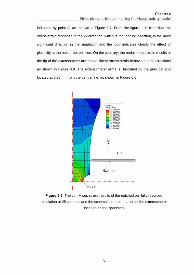
Chapter 6 _________________ Finite element simulation using the viscoplasticity model
151
indicated by point A, are shown in Figure 6.7. From the figure, it is clear that the
stress-strain response in the 22-direction, which is the loading direction, is the most
significant direction in the simulation and the loop indicates clearly the effect of
plasticity at the notch root position. On the contrary, the nodal stress-strain results at
the tip of the extensometer arm reveal linear stress-strain behaviour in all directions
as shown in Figure 6.8. The extensometer arms is illustrated by the grey pin and
located at 6.25mm from the centre line, as shown in Figure 6.6.
Figure 6.6: The von Mises stress results of the notched bar fully reversed
simulation at 25 seconds and the schematic representation of the extensometer
location on the specimen
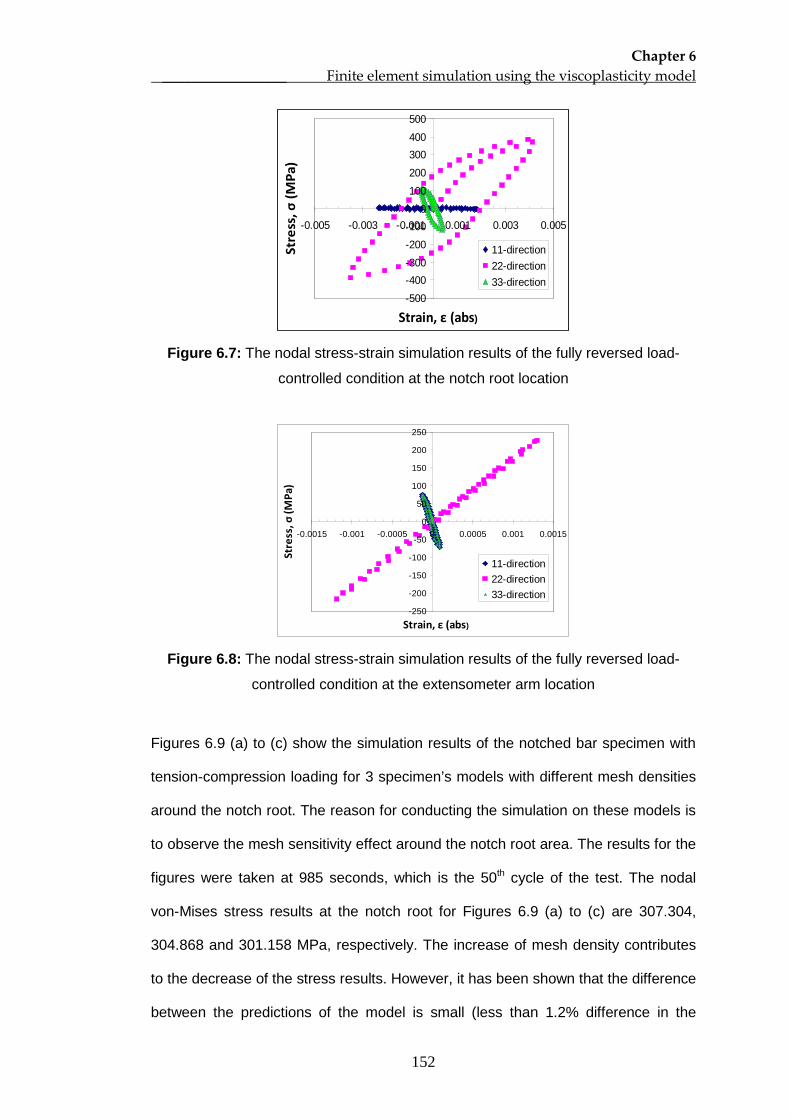
Chapter 6 _________________ Finite element simulation using the viscoplasticity model
152
Figure 6.7: The nodal stress-strain simulation results of the fully reversed load-
controlled condition at the notch root location
Figure 6.8: The nodal stress-strain simulation results of the fully reversed load-
controlled condition at the extensometer arm location
Figures 6.9 (a) to (c) show the simulation results of the notched bar specimen with
tension-compression loading for 3 specimen’s models with different mesh densities
around the notch root. The reason for conducting the simulation on these models is
to observe the mesh sensitivity effect around the notch root area. The results for the
figures were taken at 985 seconds, which is the 50th
-250
-200
-150
-100
-50
0
50
100
150
200
250
-0.0015 -0.001 -0.0005 0 0.0005 0.001 0.0015
Strain, ε (abs)
Stre
ss, σ
(MPa
)
11-direction22-direction33-direction
cycle of the test. The nodal
von-Mises stress results at the notch root for Figures 6.9 (a) to (c) are 307.304,
304.868 and 301.158 MPa, respectively. The increase of mesh density contributes
to the decrease of the stress results. However, it has been shown that the difference
between the predictions of the model is small (less than 1.2% difference in the
-500-400-300-200-100
0100200300400500
-0.005 -0.003 -0.001 0.001 0.003 0.005
Strain, ε (abs)
Stre
ss, σ
(MPa
)
11-direction22-direction33-direction
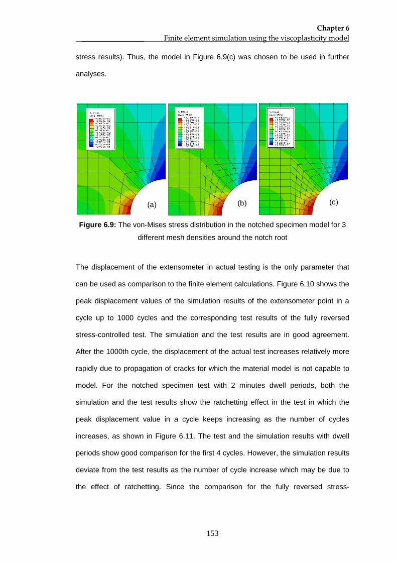
Chapter 6 _________________ Finite element simulation using the viscoplasticity model
153
stress results). Thus, the model in Figure 6.9(c) was chosen to be used in further
analyses.
Figure 6.9: The von-Mises stress distribution in the notched specimen model for 3
different mesh densities around the notch root
The displacement of the extensometer in actual testing is the only parameter that
can be used as comparison to the finite element calculations. Figure 6.10 shows the
peak displacement values of the simulation results of the extensometer point in a
cycle up to 1000 cycles and the corresponding test results of the fully reversed
stress-controlled test. The simulation and the test results are in good agreement.
After the 1000th cycle, the displacement of the actual test increases relatively more
rapidly due to propagation of cracks for which the material model is not capable to
model. For the notched specimen test with 2 minutes dwell periods, both the
simulation and the test results show the ratchetting effect in the test in which the
peak displacement value in a cycle keeps increasing as the number of cycles
increases, as shown in Figure 6.11. The test and the simulation results with dwell
periods show good comparison for the first 4 cycles. However, the simulation results
deviate from the test results as the number of cycle increase which may be due to
the effect of ratchetting. Since the comparison for the fully reversed stress-
(a) (b) (c)
Chapter 6 _________________ Finite element simulation using the viscoplasticity model
154
controlled case has shown a promising result, the simulation results may be further
used to predict the failure life of the notched specimen.
The fatigue life of the notched specimen in the fully reversed stress-controlled test
can be predicted using the energy based fatigue model. In Chapter 4, the fatigue
model is developed using the solid specimen subjected to uniaxial loading as given
in Equation 4.7. The number of cycles to failure, Nf
, in the equation is based on a 5
percent stress drop failure criterion in the strain-controlled test. By using this 5
percent criterion in the stress-controlled test of the notch specimen, during which
the displacement values increase through out the test as the P91 steel shows cyclic
softening behaviour, the number of cycles to failure is 1150 cycle as shown in
Figure 6.12.
In multiaxial cases such as the notched specimen, the plastic strain energy per
cycle can be determined from the sum of the hysteresis loop areas associated with
all components (Charkaluk, 2009). The hysteresis loop areas were determined from
the stress-strain results at the start of the stabilized period where the displacement
range increases steadily as the number of cycles increases as suggested by
Constantinescu et al. (2004). Based on the simulation results, the stabilized stage
started at the 50th cycle. The stress-strain values during the 50th cycle at the notch
root area (point A), which is the critical area for the crack initiation and growth in the
notched specimen, were used to estimate the number of cycles to failure. The
results of the nodal stress-strain at point A can be reasonably used where the
difference of the von-Mises stress results at the 985th seconds between the nodal
point and the integration point is small (less than 5 MPa). The hysteresis loop areas
were determined using the trapezoid method as described in Chapter 4. The sum of
the hysteresis loop areas, based on the nodal stress-strain results of point A, is 2.51
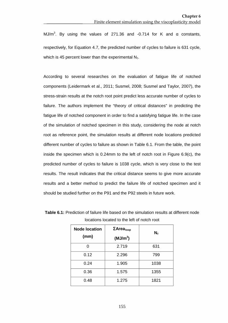
Chapter 6 _________________ Finite element simulation using the viscoplasticity model
155
MJ/m3. By using the values of 271.36 and -0.714 for K and α constants,
respectively, for Equation 4.7, the predicted number of cycles to failure is 631 cycle,
which is 45 percent lower than the experimental Nf
.
According to several researches on the evaluation of fatigue life of notched
components (Leidermark et al., 2011; Susmel, 2008; Susmel and Taylor, 2007), the
stress-strain results at the notch root point predict less accurate number of cycles to
failure. The authors implement the “theory of critical distances” in predicting the
fatigue life of notched component in order to find a satisfying fatigue life. In the case
of the simulation of notched specimen in this study, considering the node at notch
root as reference point, the simulation results at different node locations predicted
different number of cycles to failure as shown in Table 6.1. From the table, the point
inside the specimen which is 0.24mm to the left of notch root in Figure 6.9(c), the
predicted number of cycles to failure is 1038 cycle, which is very close to the test
results. The result indicates that the critical distance seems to give more accurate
results and a better method to predict the failure life of notched specimen and it
should be studied further on the P91 and the P92 steels in future work.
Table 6.1: Prediction of failure life based on the simulation results at different node
locations located to the left of notch root
Node location (mm)
ΣArea
(MJ/m
loop
3N
) f
0 2.719 631
0.12 2.296 799
0.24 1.905 1038
0.36 1.575 1355
0.48 1.275 1821
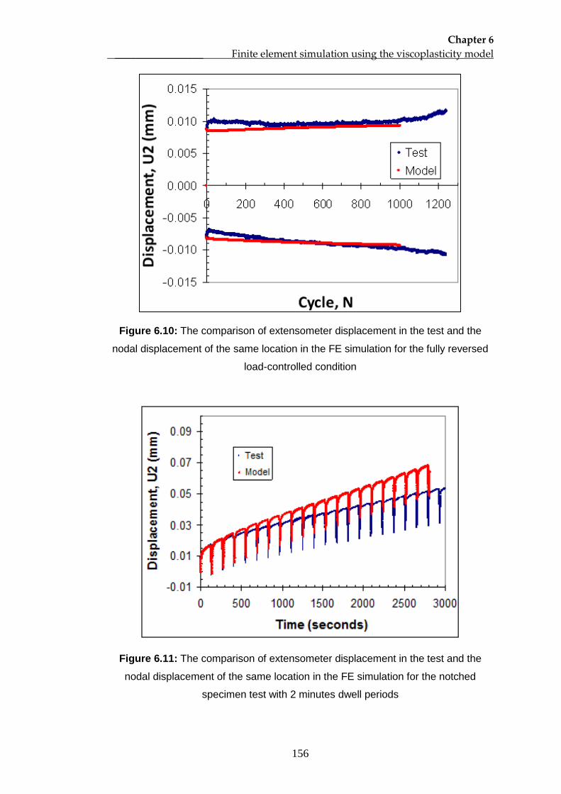
Chapter 6 _________________ Finite element simulation using the viscoplasticity model
156
Figure 6.10: The comparison of extensometer displacement in the test and the
nodal displacement of the same location in the FE simulation for the fully reversed
load-controlled condition
Figure 6.11: The comparison of extensometer displacement in the test and the
nodal displacement of the same location in the FE simulation for the notched
specimen test with 2 minutes dwell periods
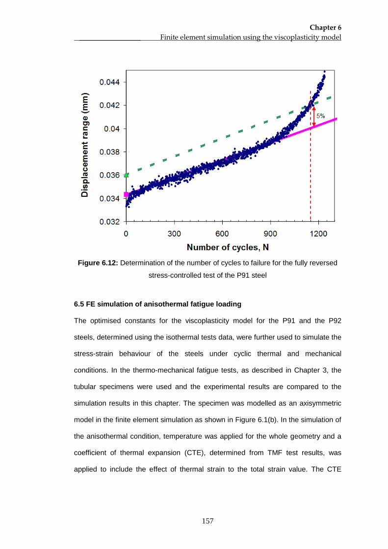
Chapter 6 _________________ Finite element simulation using the viscoplasticity model
157
Figure 6.12: Determination of the number of cycles to failure for the fully reversed
stress-controlled test of the P91 steel
6.5 FE simulation of anisothermal fatigue loading
The optimised constants for the viscoplasticity model for the P91 and the P92
steels, determined using the isothermal tests data, were further used to simulate the
stress-strain behaviour of the steels under cyclic thermal and mechanical
conditions. In the thermo-mechanical fatigue tests, as described in Chapter 3, the
tubular specimens were used and the experimental results are compared to the
simulation results in this chapter. The specimen was modelled as an axisymmetric
model in the finite element simulation as shown in Figure 6.1(b). In the simulation of
the anisothermal condition, temperature was applied for the whole geometry and a
coefficient of thermal expansion (CTE), determined from TMF test results, was
applied to include the effect of thermal strain to the total strain value. The CTE
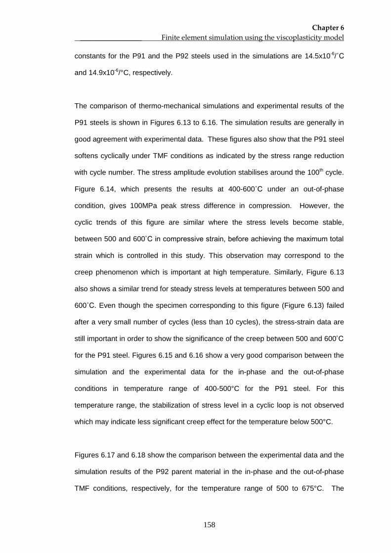
Chapter 6 _________________ Finite element simulation using the viscoplasticity model
158
constants for the P91 and the P92 steels used in the simulations are 14.5x10⁻⁶/˚C
and 14.9x10⁻⁶
/°C, respectively.
The comparison of thermo-mechanical simulations and experimental results of the
P91 steels is shown in Figures 6.13 to 6.16. The simulation results are generally in
good agreement with experimental data. These figures also show that the P91 steel
softens cyclically under TMF conditions as indicated by the stress range reduction
with cycle number. The stress amplitude evolution stabilises around the 100th
cycle.
Figure 6.14, which presents the results at 400-600˚C under an out-of-phase
condition, gives 100MPa peak stress difference in compression. However, the
cyclic trends of this figure are similar where the stress levels become stable,
between 500 and 600˚C in compressive strain, before achieving the maximum total
strain which is controlled in this study. This observation may correspond to the
creep phenomenon which is important at high temperature. Similarly, Figure 6.13
also shows a similar trend for steady stress levels at temperatures between 500 and
600˚C. Even though the specimen corresponding to this figure (Figure 6.13) failed
after a very small number of cycles (less than 10 cycles), the stress-strain data are
still important in order to show the significance of the creep between 500 and 600˚C
for the P91 steel. Figures 6.15 and 6.16 show a very good comparison between the
simulation and the experimental data for the in-phase and the out-of-phase
conditions in temperature range of 400-500°C for the P91 steel. For this
temperature range, the stabilization of stress level in a cyclic loop is not observed
which may indicate less significant creep effect for the temperature below 500°C.
Figures 6.17 and 6.18 show the comparison between the experimental data and the
simulation results of the P92 parent material in the in-phase and the out-of-phase
TMF conditions, respectively, for the temperature range of 500 to 675°C. The
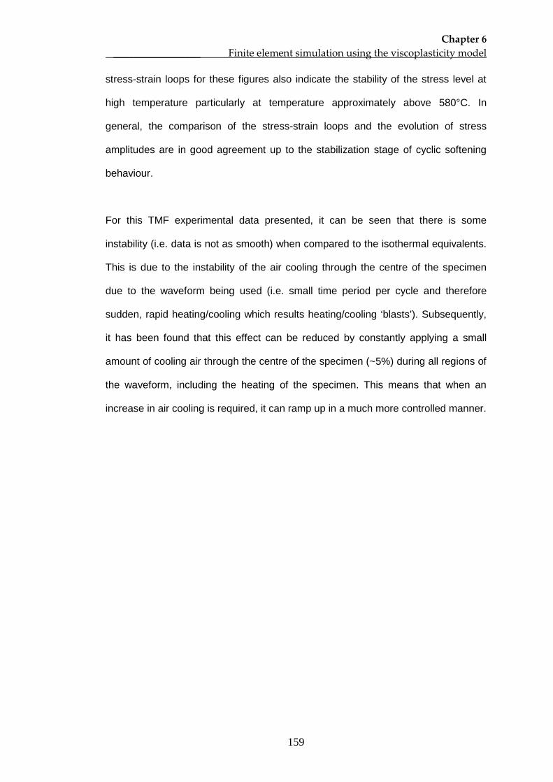
Chapter 6 _________________ Finite element simulation using the viscoplasticity model
159
stress-strain loops for these figures also indicate the stability of the stress level at
high temperature particularly at temperature approximately above 580°C. In
general, the comparison of the stress-strain loops and the evolution of stress
amplitudes are in good agreement up to the stabilization stage of cyclic softening
behaviour.
For this TMF experimental data presented, it can be seen that there is some
instability (i.e. data is not as smooth) when compared to the isothermal equivalents.
This is due to the instability of the air cooling through the centre of the specimen
due to the waveform being used (i.e. small time period per cycle and therefore
sudden, rapid heating/cooling which results heating/cooling ‘blasts’). Subsequently,
it has been found that this effect can be reduced by constantly applying a small
amount of cooling air through the centre of the specimen (~5%) during all regions of
the waveform, including the heating of the specimen. This means that when an
increase in air cooling is required, it can ramp up in a much more controlled manner.
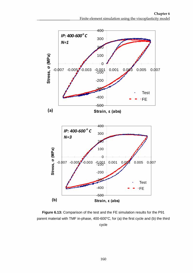
Chapter 6 _________________ Finite element simulation using the viscoplasticity model
160
-500
-400
-300
-200
-100
0
100
200
300
400
-0.007 -0.005 -0.003 -0.001 0.001 0.003 0.005 0.007
Strain, ε (abs)
Stre
ss, σ
(MPa
)
TestFE
IP: 400-600o CN=1
(a)
-500
-400
-300
-200
-100
0
100
200
300
400
-0.007 -0.005 -0.003 -0.001 0.001 0.003 0.005 0.007
Strain, ε (abs)
Stre
ss, σ
(MPa
)
TestFE
IP: 400-600 o CN=3
(b)
Figure 6.13: Comparison of the test and the FE simulation results for the P91
parent material with TMF in-phase, 400-600°C, for (a) the first cycle and (b) the third
cycle
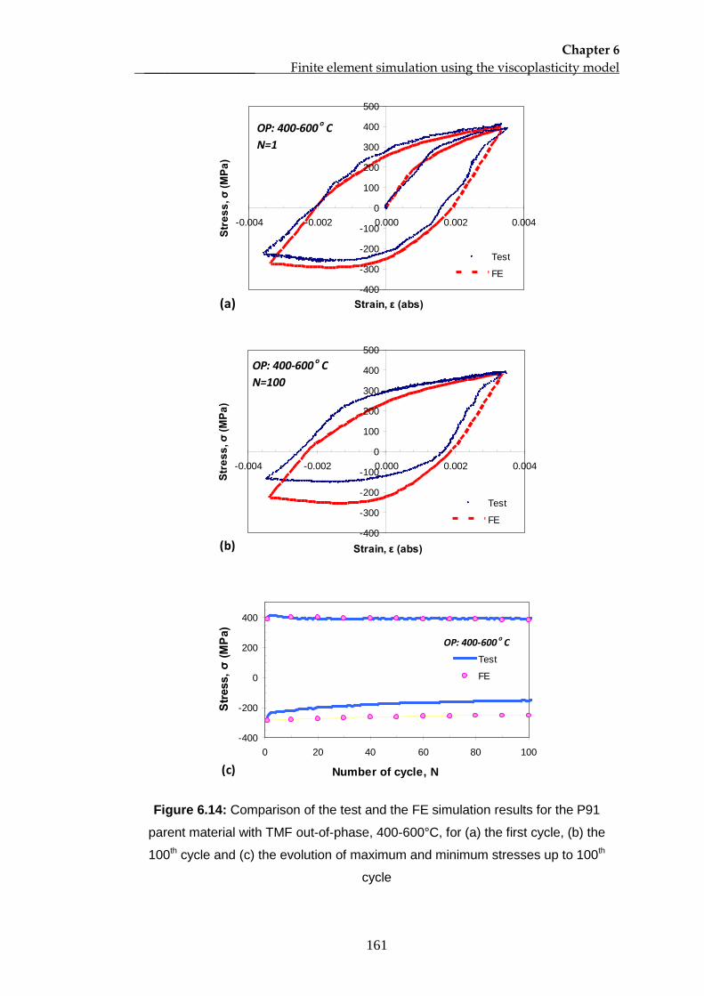
Chapter 6 _________________ Finite element simulation using the viscoplasticity model
161
-400
-300
-200
-100
0
100
200
300
400
500
-0.004 -0.002 0.000 0.002 0.004
Strain, ε (abs)
Stre
ss, σ
(MPa
)
Test
FE
OP: 400-600 o CN=1
(a)
-400
-300
-200
-100
0
100
200
300
400
500
-0.004 -0.002 0.000 0.002 0.004
Strain, ε (abs)
Stre
ss, σ
(MPa
)
Test
FE
OP: 400-600 o CN=100
(b)
-400
-200
0
200
400
0 20 40 60 80 100
Number of cycle, N
Stre
ss, σ
(MPa
)
Test
FE
OP: 400-600 o C
(c)
Figure 6.14: Comparison of the test and the FE simulation results for the P91
parent material with TMF out-of-phase, 400-600°C, for (a) the first cycle, (b) the
100th cycle and (c) the evolution of maximum and minimum stresses up to 100th
cycle
Chapter 6 _________________ Finite element simulation using the viscoplasticity model
162
-500
-400
-300
-200
-100
0
100
200
300
400
500
-0.006 -0.004 -0.002 0 0.002 0.004 0.006
Strain, ε (abs)
Stre
ss, σ
(MPa
)
Test
FE
IP: 400-500 o CN=1
(a)
-500
-400
-300
-200
-100
0
100
200
300
400
500
-0.006 -0.004 -0.002 0.000 0.002 0.004 0.006
Strain, ε (abs)
Stre
ss, σ
(MPa
)
Test
FE
IP: 400-500 o CN=100
(b)
-500
-300
-100
100
300
500
0 20 40 60 80 100
Number of cycle, N
Stre
ss, σ
(MPa
)
Test
FE
IP: 400-500 o C
(c)
Figure 6.15: Comparison of the test and the FE simulation results for the P91
parent material with TMF in-phase, 400-500°C, for (a) the first cycle, (b) the 100th
cycle and (c) the evolution of maximum and minimum stresses up to 100th cycle
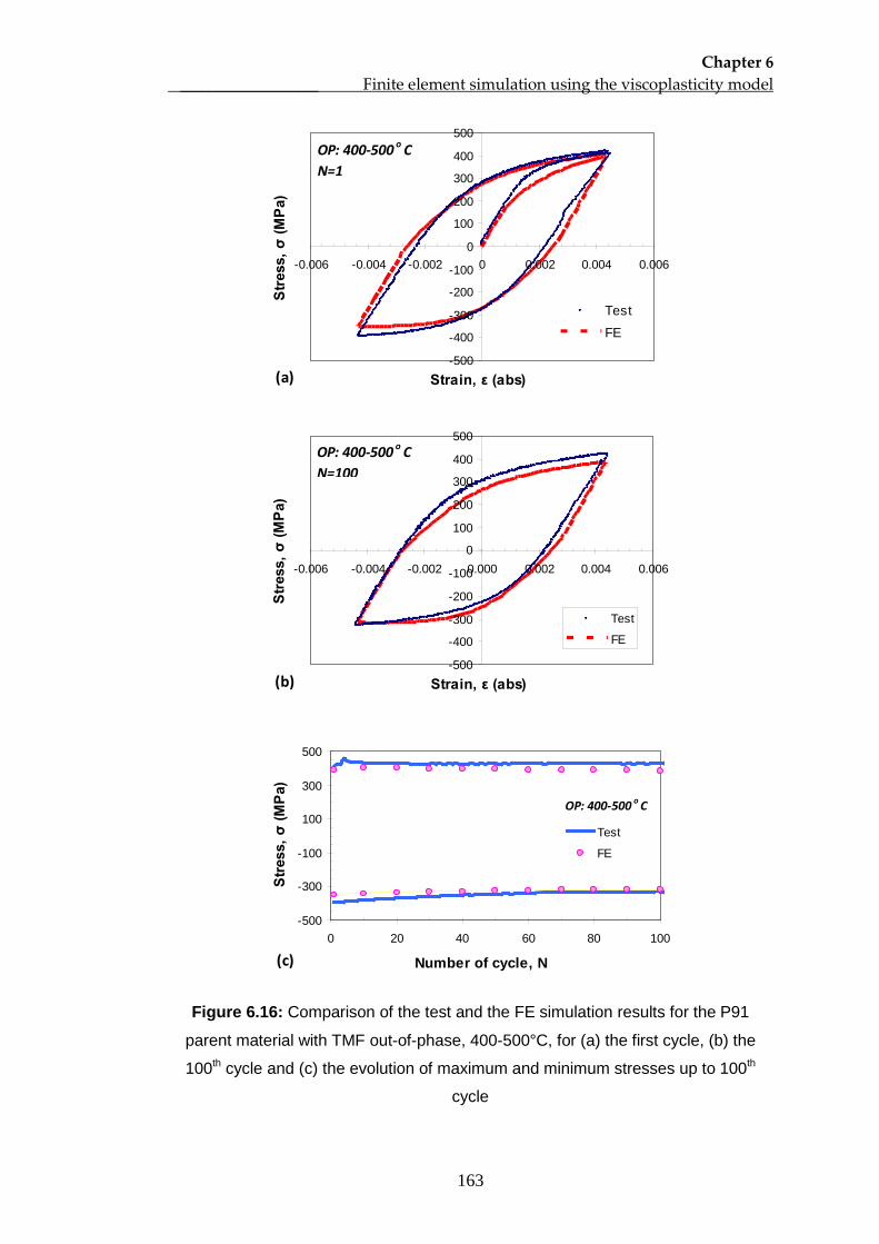
Chapter 6 _________________ Finite element simulation using the viscoplasticity model
163
-500
-400
-300
-200
-100
0
100
200
300
400
500
-0.006 -0.004 -0.002 0 0.002 0.004 0.006
Strain, ε (abs)
Stre
ss, σ
(MPa
)
Test
FE
OP: 400-500 o CN=1
(a)
-500
-400
-300
-200
-100
0
100
200
300
400
500
-0.006 -0.004 -0.002 0.000 0.002 0.004 0.006
Strain, ε (abs)
Stre
ss, σ
(MPa
)
Test
FE
OP: 400-500 o CN=100
(b)
-500
-300
-100
100
300
500
0 20 40 60 80 100
Number of cycle, N
Stre
ss, σ
(MPa
)
Test
FE
OP: 400-500 o C
(c)
Figure 6.16: Comparison of the test and the FE simulation results for the P91
parent material with TMF out-of-phase, 400-500°C, for (a) the first cycle, (b) the
100th cycle and (c) the evolution of maximum and minimum stresses up to 100th
cycle
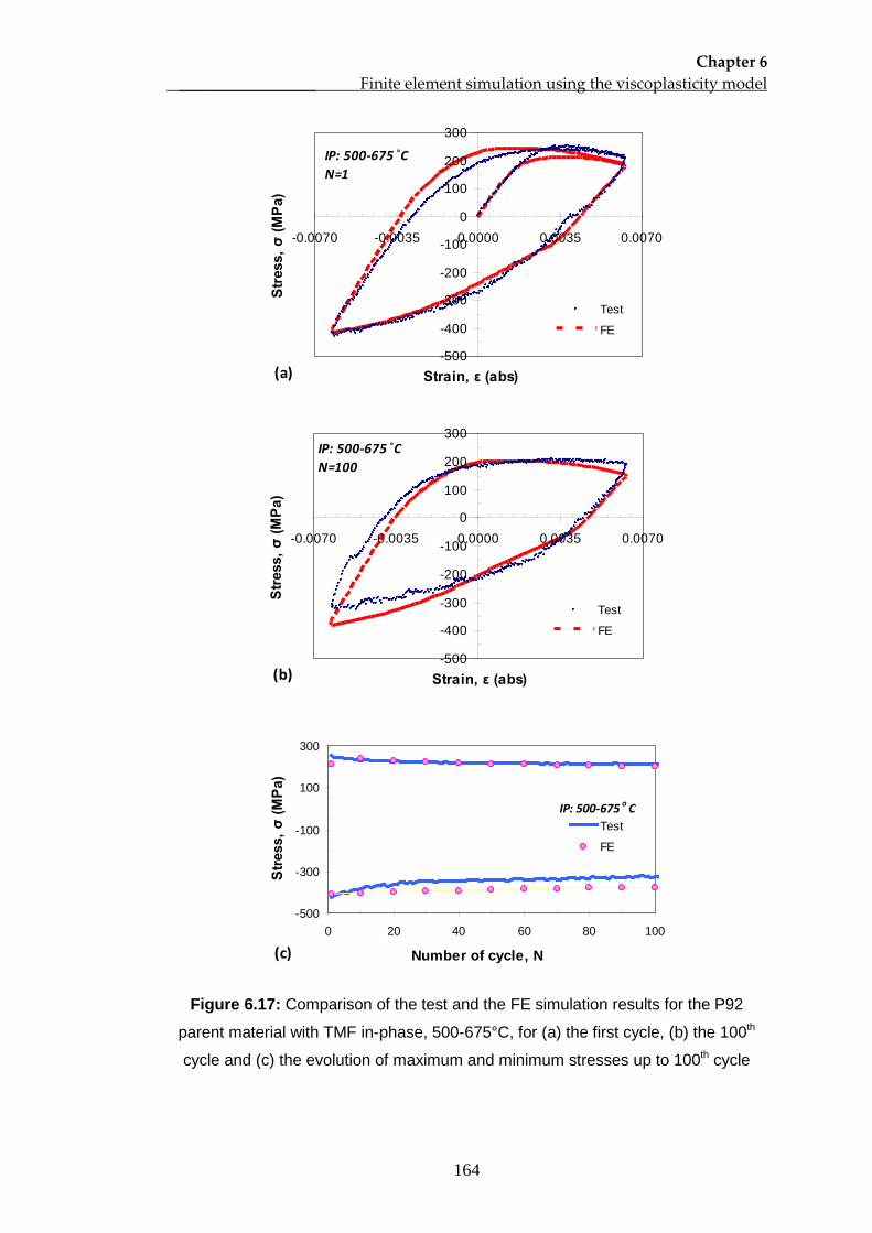
Chapter 6 _________________ Finite element simulation using the viscoplasticity model
164
-500
-400
-300
-200
-100
0
100
200
300
-0.0070 -0.0035 0.0000 0.0035 0.0070
Strain, ε (abs)
Stre
ss, σ
(MPa
)
Test
FE
IP: 500-675 ˚CN=1
(a)
-500
-400
-300
-200
-100
0
100
200
300
-0.0070 -0.0035 0.0000 0.0035 0.0070
Strain, ε (abs)
Stre
ss, σ
(MPa
)
Test
FE
IP: 500-675 ˚CN=100
(b)
-500
-300
-100
100
300
0 20 40 60 80 100
Number of cycle, N
Stre
ss, σ
(MPa
)
Test
FE
IP: 500-675 o C
(c)
Figure 6.17: Comparison of the test and the FE simulation results for the P92
parent material with TMF in-phase, 500-675°C, for (a) the first cycle, (b) the 100th
cycle and (c) the evolution of maximum and minimum stresses up to 100th
cycle
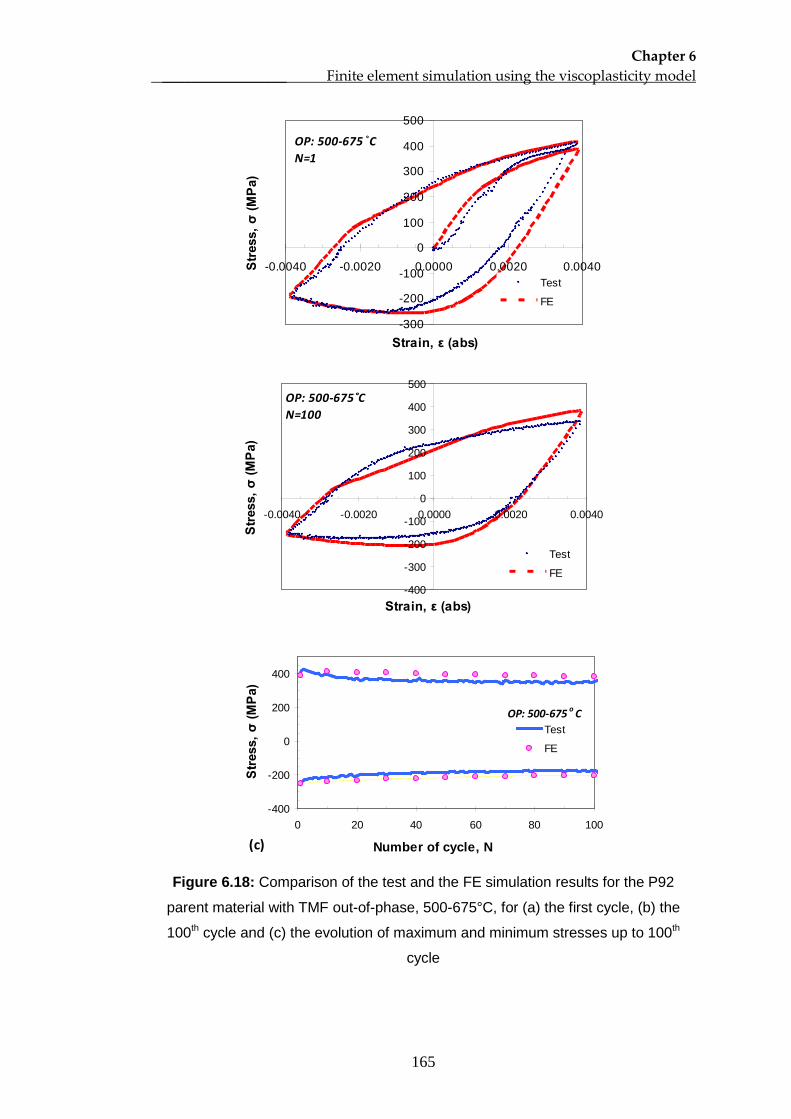
Chapter 6 _________________ Finite element simulation using the viscoplasticity model
165
-300
-200
-100
0
100
200
300
400
500
-0.0040 -0.0020 0.0000 0.0020 0.0040
Strain, ε (abs)
Stre
ss, σ
(MPa
)
Test
FE
OP: 500-675 ˚CN=1
-400
-300
-200
-100
0
100
200
300
400
500
-0.0040 -0.0020 0.0000 0.0020 0.0040
Strain, ε (abs)
Stre
ss, σ
(MPa
)
Test
FE
OP: 500-675˚CN=100
-400
-200
0
200
400
0 20 40 60 80 100
Number of cycle, N
Stre
ss, σ
(MPa
)
Test
FE
OP: 500-675 o C
(c)
Figure 6.18: Comparison of the test and the FE simulation results for the P92
parent material with TMF out-of-phase, 500-675°C, for (a) the first cycle, (b) the
100th cycle and (c) the evolution of maximum and minimum stresses up to 100th
cycle
Chapter 6 _________________ Finite element simulation using the viscoplasticity model
166
6.6 Conclusions
This chapter has presented the simulation results of the P91 and the P92 steel
behaviour using the viscoplasticity model. The following conclusions can be drawn
from this chapter:
• The simulation of the viscoplasticity model, developed by using data from
high strain amplitude tests, gives good stress-strain comparison to the lower
strain amplitudes.
• The simulation results of the notched specimen indicate the capability of the
model to predict the stress-strain behaviour in multiaxial conditions. The
prediction of the notched specimen’s failure life can be further improved by
implementing the critical distance theory.
• Identification of viscoplasticity constants using data from the isothermal tests
gives good comparison to the thermo-mechanical behaviour.
• All the simulation results show cyclic softening behaviour where the stress
amplitude decreases in a strain-controlled test while the strain amplitude
increases in the stress-controlled test. The nonlinear evolution of cyclic
parameters (i.e. stress or strain amplitude) in the initial cyclic period and
then the stabilisation of the parameters have been modelled satisfactorily by
the developed viscoplasticity model.
Chapter 7 ________ ____________________________________ Conclusions and future work
167
Chapter 7 – Conclusions and future work
The research has focussed on the testing and the development of a material
constitutive model of the P91 and the P92 steels under thermo-mechanical fatigue
condition at high temperature. Based on the stress-strain data obtained in the test,
the sets of material constants for the viscoplasticity models of the steels have been
determined and the constants can be used in a commercial finite element software
for further analysis.
7.1 Conclusions
The cyclic loading tests on the P91 and the P92 steels have been performed on
three types of specimens in isothermal and anisothermal conditions using the
Instron 8862 TMF testing system. The temperature gradient along the gauge
section of the specimens was controlled to within ±10°C of the target temperature.
The main thermocouple, which controls the temperature of the test specimen, was
instrumented on the shoulder of specimen initially in order to avoid crack initiation at
the welding point of thermocouple wires. It has been found that in most cases the
instrumentation of the main thermocouple in the middle of gauge section with a low
possible current during spot welding will not initiate cracks at the welding point of
thermocouple wires.
The results of the cyclic loading tests of the steels at high temperature exhibit cyclic
softening behaviour with three distinct stages. The stages of one to three represent
rapid cyclic softening followed by a stabilisation period and finally a crack growth
stage. The mechanical parameters, such as the plastic strain range, the stress
range and the hysteresis loop area, show a stabilised condition in the second stage
of cyclic softening. The softening behaviour is associated with the coarsening of the
Chapter 7 ________ ____________________________________ Conclusions and future work
168
subgrains and it has been observed in the microstructural investigations of the cyclic
loading specimens at different life fractions. The coarsening of the subgrains occurs
rapidly in the first stage of cyclic softening and it slowly continues in the second and
the third stage. The microstructural evolutions during the first two stages of cyclic
softening do not significantly cause damage to the steels as indicated by the plot of
Young’s modulus. The initiation of cracks at the end of the stabilisation stage
indicates the starting point of the significant material’s damage and the load bearing
capacity of the steel decreases as a consequence of macro crack development in
the third stage of softening.
The viscoplasticity models for the P91 and the P92 steels have been developed and
the stress-strain predictions have shown good comparison to experimental data,
particularly in temperature range of 400 to 600°C and 500 to 675°C respectively.
The material constants were initially estimated from the tension-compression test
data. The implementation of the optimisation programme significantly improves the
accuracy of stress-strain predictions of the viscoplasticity model. The constants give
very good predictions of the stress-strain behaviour in cyclic stress-strain conditions
up to about half the number of cycles to failure. The model also gives reasonably
good predictions of stress relaxation behaviour. The stress-strain behaviour
predictions of the stabilisation stage has been further improved by using the
combined linear and nonlinear isotropic hardening model and consequently the
viscoplasticity model is capable of predicting stress-strain softening behaviour up to
the end of stabilisation stage.
The finite element simulation using the viscoplasticity model has been implemented
in ABAQUS software with an external material library software called Zmat. The
simulation results of the behaviour of the steels with various strain ranges, cyclic
Chapter 7 ________ ____________________________________ Conclusions and future work
169
thermo-mechanical conditions and notched geometry show good comparison to the
experimental data. The promising predictive capability indicates that the model can
be used in cyclic thermo-mechanical conditions and under multiaxial stress states at
high temperature. The simulation of notched specimen indicates the requirement to
select the stress-strain data at a point near the notch root in order to predict better
failure lives.
7.2 Future work
Based on the research work presented in this study, some potential work can be
further implemented in order to improve and extend the current work in the future as
follows:
• Repetition of test should be implemented, which depends on the availability
of specimens, in order to check the scatter of the experimental data. The
repetition of test can also increase the level of confidence for the
determination of the number of cycles to failure, particularly for the thermo-
mechanical fatigue tests in which the trend of stress amplitude evolution of
the third stages of cyclic softening seems inconsistent between the TMF
tests.
• The understanding of the steels behaviour and the capability of the
viscoplasticity model can be further improved by conducting the strain rate
effect and ratchetting behaviour in the future research. However, the
consideration of this kind of behaviour will require more specimens in the
testing programme.
• The microstructural investigation of the interrupted cyclic tests specimens
using the transmission electron microscope should be further studied by
focussing on the dislocation density evolution. The statistically
representative data, such as the misorientation angles, should be also
Chapter 7 ________ ____________________________________ Conclusions and future work
170
studied by using the electron microscope with electron backscattered
diffraction (EBSD) capability in order to support the research finding
quantitatively. However, this work is more relevant to specific research on
the metallurgy of the steels.
• The optimisation programme can be further improved by considering more
than one set of test data as the objective functions so that the programme
can produce the optimised constants which give good prediction for different
set of loading types. The current optimisation programme only considers one
set of experimental data in each optimisation process.
• The two-stage isotropic hardening equation can be included in the current
optimisation programme in order to obtain optimised material constants
which can predict good stress-strain behaviour up to the end of stabilised
stage of the cyclic softening of the steels.
• The finite element prediction of welded pipes, which consist of parent
material and weld metal, subjected to realistic thermo-mechanical fatigue
loading can be implemented to observe the stress-strain behaviour in real
components of power plant.
• The experimental works on the determination of critical distance in a notched
specimen should be implemented in order to improve the understanding of
the stress-strain behaviour in the notched specimen and predict better
number of cycles to failure.
171
REFERENCES ABE, F., KERN, T.-U. & VISWANATHAN, R. (2008) Creep resistant steels,
Cambridge, Woodhead Publishing. ARMAS, A. F., PETERSEN, C., SCHMITT, R., AVALOS, M. & ALVAREZ, I. (2004)
Cyclic instability of martensite laths in reduced activation ferritic/martensitic steels. Journal of Nuclear Materials, 329-333, 252-256.
AVANZINI, A. (2008) Mechanical characterization and finite element modelling of
cyclic stress-strain behaviour of ultra high molecular weight polyethylene. Materials & Design, 29, 330-343.
BARI, S. & HASSAN, T. (2000) Anatomy of coupled constitutive models for
ratcheting simulation. International Journal of Plasticity, 16, 381-409. BECK, T. & RAU, K. (2008) Temperature measurement and control methods in
TMF testing – a comparison and evaluation. International Journal of Fatigue, 30, 226-233.
BENDICK, W., CIPOLLA, L., GABREL, J. & HALD, J. (2010) New ECCC
assessment of creep rupture strength for steel grade X10CrMoVNb9-1 (Grade 91). International Journal of Pressure Vessels and Piping, 87, 304-309.
BERNHART, G., MOULINIER, G., BRUCELLE, O. & DELAGNES, D. (1999) High
temperature low cycle fatigue behaviour of a martensitic forging tool steel. International Journal of Fatigue, 21, 179-186.
BHADESHIA, H. K. D. H. (2003) Mechanisms and Models for Creep Deformation
and Rupture. IN MILNE, I., RITCHIE, R. O. & KARIHALOO, B. (Eds.) Comprehensive Structural Integrity. Oxford, Pergamon.
BILLO, E. J. (2007) Excel for scienctists and engineers: numerical methods, New
Jersey, John Wiley & Sons. BRETT, S. J. (2003) Service experience of weld cracking in CrMoV steam pipework
systems. 2nd International Conference on Integrity of High Temperature Welds. London.
BRETT, S. J. (2007) UK experience with modified 9Cr (grade 91) steel. VTT
Symposium (Valtion Teknillinen Tutkimuskeskus), 1, 48-60. CALLISTER, W. D. (2000) Materials science and engineering: an introduction, New
York, John Wiley & Sons. CHABOCHE, J. L. (1986) Time-independent constitutive theories for cyclic
plasticity. International Journal of Plasticity, 2, 149-188. CHABOCHE, J. L. (1989) Constitutive equations for cyclic plasticity and cyclic
viscoplasticity. International Journal of Plasticity, 5, 247-302. CHABOCHE, J. L. (2001) Unified Model of Cyclic Viscoplasticity Based on the
Nonlinear Kinematic Hardening Rule. IN LEMAITRE, J. (Ed.) Handbook of Materials Behavior Models. Burlington, Academic Press.
172
CHABOCHE, J. L. (2008) A review of some plasticity and viscoplasticity constitutive
theories. International Journal of Plasticity, 24, 1642-1693. CHABOCHE, J. L. & ROUSSELIER, G. (1983) On the Plastic and Viscoplastic
Constitutive Equations - Part 1: Rules Developed With Internal Variable Concept. Journal of Pressure Vessel Technology, 105, 153-159.
CHABOCHE, J. L. & GALLERNEAU, F. (2001) An overview of the damage
approach of durability modelling at elevated temperature. Fatigue and Fracture of Engineering Materials and Structures, 24, 405-418.
CHARKALUK, E., BIGNONNET, A., CONSTANTINESCU, A. & DANG VAN, K.
(2002) Fatigue design of structures under thermomechanical loadings. Fatigue and Fracture of Engineering Materials and Structures, 25, 1199-1206.
CHARKALUK, E. (2009) Energy as a damage factor in fatigue: Plenary lecture at
the international conference low cycle fatigue 6. Materialpruefung/Materials Testing, 51, 269-275.
CHARKALUK, E. & CONSTANTINESCU, A. (2000) Energetic approach in
thermomechanical fatigue for silicon molybdenum cast iron. Materials at High Temperatures, 17, 373-380.
CHUN, B. K., JINN, J. T. & LEE, J. K. (2002) Modeling the Bauschinger effect for
sheet metals, part I: theory. International Journal of Plasticity, 18, 571-595. CONSTANTINESCU, A., CHARKALUK, E., LEDERER, G. & VERGER, L. (2004) A
computational approach to thermomechanical fatigue. International Journal of Fatigue, 26, 805-818.
DESHPANDE, A. A., LEEN, S. B. & HYDE, T. H. (2010a) Finite element prediction
of creep-plastic ratchetting and low cycle creep-fatigue for a large SPF tool. Journal of Materials Engineering and Performance, 19, 452-466.
DESHPANDE, A. A., LEEN, S. B., SUN, W. & HYDE, T. H. (2010) Thermo-
mechanical analysis and lifing of Ni-Cr SPF tool. International Journal of Material Forming, 3, 1151-1154.
DESHPANDE, A. A., LEEN, S. B. & HYDE, T. H. (2008) Finite element based
predictions of life limiting behaviour for a large SPF tool. Materialwissenschaft und Werkstofftechnik, 39, 309-316.
DUBEY, J. S., CHILUKURU, H., CHAKRAVARTTY, J. K., SCHWIENHEER, M.,
SCHOLZ, A. & BLUM, W. (2005) Effects of cyclic deformation on subgrain evolution and creep in 9-12% Cr-steels. Materials Science and Engineering: A, 406, 152-159.
DUNNE, F. & PETRINIC, N. (2005) Introduction to computational plasticity, Oxford,
Oxford University Press. DUNNE, F. P. E. & HAYHURST, D. R. (1992a) Continuum damage based
constitutive equations for copper under high temperature creep and cyclic plasticity. Proceedings of the Royal Society: Mathematical and Physical Sciences, 437, 545-566.
173
DUNNE, F. P. E. & HAYHURST, D. R. (1992b) Modelling of combined high-
temperature creep and cyclic plasticity in components using continuum damage mechanics. Proceedings of the Royal Society: Mathematical and Physical Sciences, 437, 567-589.
DUNNE, F. P. E., MAKIN, J. & HAYHURST, D. R. (1992) Automated procedures for
the determination of high temperature viscoplastic damage constitutive equations. Proceedings of the Royal Society: Mathematical and Physical Sciences, 437, 527-544.
EL GHARAD, A., ZEDIRA, H., AZARI, Z. & PLUVINAGE, G. (2006) A synergistic
creep fatigue failure model damage (case of the alloy Z5NCTA at 550 °C). Engineering Fracture Mechanics, 73, 750-770.
ELLYIN, F. & KUJAWSKI, D. (1984) Plastic strain energy in fatigue failure. Journal
of Pressure Vessel Technology, Transactions of the ASME, 106, 342-347. ENNIS, P. J. & CZYRSKA-FILEMONOWICZ, A. (2003) Recent advances in creep-
resistant steels for power plant applications. Sadhana - Academy Proceedings in Engineering Sciences, 28, 709-730.
ESSMANN, U. & MUGHRABI, H. (1979) ANNIHILATION OF DISLOCATIONS
DURING TENSILE AND CYCLIC DEFORMATION AND LIMITS OF DISLOCATION DENSITIES. Philosophical Magazine A: Physics of Condensed Matter, Structure, Defects and Mechanical Properties, 40, 731-756.
EVANS, R. W. & WILSHERE, B. (1985) Creep of metals and alloys, London,
Institute of Metals. FAULKNER, R. G. (2008) Grain boundaries in creep-resistant steels. IN ABE, F.,
KERN, T.-U. & VISWANATHAN, R. (Eds.) Creep-resistant steels. Cambridge, Woodhead Publishing, CRC Press.
FIGIEL, L. & GÜNTHER, B. (2008) Modelling the high-temperature
longitudinal fatigue behaviour of metal matrix composites (SiC/Ti-6242): Nonlinear time-dependent matrix behaviour. International Journal of Fatigue, 30, 268-276.
FOURNIER, B., SAUZAY, M., CAËS, C., NOBLECOURT, M. & MOTTOT, M. (2006)
Analysis of the hysteresis loops of a martensitic steel: Part I: Study of the influence of strain amplitude and temperature under pure fatigue loadings using an enhanced stress partitioning method. Materials Science and Engineering: A, 437, 183-196.
FOURNIER, B., SAUZAY, M., CAËS, C., NOBLECOURT, M., MOTTOT, M.,
ALLAIS, L., TOURNIE, I. & PINEAU, A. (2009a) Creep-Fatigue Interactions in a 9 Pct Cr-1 Pct Mo Martensitic Steel: Part I. Mechanical Test Results. Metallurgical and Materials Transactions A, 40, 321-329.
FOURNIER, B., SAUZAY, M., BARCELO, F., RAUCH, E., RENAULT, A., COZZIKA,
T., DUPUY, L. & PINEAU, A. (2009b) Creep-Fatigue Interactions in a 9 Pct Cr-1 Pct Mo Martensitic Steel: Part II. Microstructural Evolutions. Metallurgical and Materials Transactions A, 40, 330-341.
174
FOURNIER, B., DALLE, F., SAUZAY, M., LONGOUR, J., SALVI, M., CAES, C., TOURNIE, I., GIROUX, P. F. & KIM, S. H. (2011a) Comparison of various 9-12%Cr steels under fatigue and creep-fatigue loadings at high temperature. Materials Science and Engineering A, 528, 6934-6945.
FOURNIER, B., SAUZAY, M. & PINEAU, A. (2011b) Micromechanical model of the
high temperature cyclic behaviour of 9-12%Cr martensitic steels. International Journal of Plasticity, 27, 1803-1816.
FREDERICK, C. O. & ARMSTRONG, P. J. (2007) A mathematical representation of
the multiaxial Bauschinger effect. Materials at High Temperatures, 24, 1-26. GONG, Y. P., HYDE, C. J., SUN, W. & HYDE, T. H. (2010) Determination of
material properties in the Chaboche unified viscoplasticity model Proceedings of the Institution of Mechanical Engineers, Part L: Journal of Materials: Design and Applications, 224, 19-29.
HAARMANN, K., VAILLANT, J. C., VANDENBERGHE, B., BENDICK, W. & ARBAB,
A. (2002) The T91/P91 book, Vallourec & Mannesmann Tubes. HÄHNER, P., RINALDI, C., BICEGO, V., AFFELDT, E., BRENDEL, T.,
ANDERSSON, H., BECK, T., KLINGELHÖFFER, H., KÜHN, H.-J., KÖSTER, A., LOVEDAY, M., MARCHIONNI, M. & RAE, C. (2008) Research and development into a European code-of-practice for strain-controlled thermo-mechanical fatigue testing. International Journal of Fatigue, 30, 372-381.
HALD, J. (2008) Microstructure and long-term creep properties of 9-12% Cr steels.
International Journal of Pressure Vessels and Piping, 85, 30-37. HALES, R., HOLDSWORTH, S. R., O'DONNELL, M. P., PERRIN, I. J. & SKELTON,
R. P. (2002) A code of practice for the determination of cyclic stress-strain data. Materials at High Temperatures, 19, 165-185.
HARTROTT, P. V., HOLMSTROM, S., CAMINADA, S. & PILLOT, S. (2009) Life-
time prediction for advanced low alloy steel P23. Materials Science and Engineering A, 510-511, 175-179.
HAYHURST, R. J., MUSTATA, R. & HAYHURST, D. R. (2005) Creep constitutive
equations for parent, Type IV, R-HAZ, CG-HAZ and weld material in the range 565-640 °C for Cr-Mo-V weldments. International Journal of Pressure Vessels and Piping, 82, 137-144.
HAYHURST, D. R., LIN, J. & HAYHURST, R. J. (2008) Failure in notched tension
bars due to high-temperature creep: Interaction between nucleation controlled cavity growth and continuum cavity growth. International Journal of Solids and Structures, 45, 2233-2250.
HERTZBERG, R. W. (1996) Deformation and fracture mechanics of engineering
materials, New York, John Wiley & Sons. HOLDSWORTH, S. (2010) Creep-fatigue interaction in power plant steels. HIDA-5
International Conference, 23-25 June 2010, Guildford, UK. HYDE, C. J., SUN, W. & LEEN, S. B. (2010) Cyclic thermo-mechanical material
modelling and testing of 316 stainless steel. International Journal of Pressure Vessels and Piping, 87, 365-372.
175
HYDE, C. J. (2010) Thermo-mechanical fatigue and creep of high temperature
materials. University of Nottingham. HYDE, T. H., SUN, W. & WILLIAMS, J. A. (2003) Creep analysis of pressurized
circumferential pipe weldments - A review. Journal of Strain Analysis for Engineering Design, 38, 1-30.
HYDE, T. H., BECKER, A. A., SUN, W. & WILLIAMS, J. A. (2006) Finite-element
creep damage analyses of P91 pipes. International Journal of Pressure Vessels and Piping, 83, 853-863.
IGARASHI, M. (2008) Alloy design philosophy of creep-resistant steel. IN ABE, F.,
KERN, T.-U. & VISWANATHAN, R. (Eds.) Creep-resistant steels. Cambridge, Woodhead Publishing, CRC Press.
JIANG, Y. & KURATH, P. (1996) Characteristics of the Armstrong-Frederick type
plasticity models. International Journal of Plasticity, 12, 387-415. JIANG, Y. & ZHANG, J. (2008) Benchmark experiments and characteristic cyclic
plasticity deformation. International Journal of Plasticity, 24, 1481-1515. KICHENIN, J., VAN, K. D. & BOYTARD, K. (1996) Finite-element simulation of a
new two-dissipative mechanisms model for bulk medium-density polyethylene. Journal of Material Science, 31, 1653-1661.
KIM, T.-W., KANG, D.-H., YEOM, J.-T. & PARK, N.-K. (2007) Continuum damage
mechanics-based creep-fatigue-interacted life prediction of nickel-based superalloy at high temperature. Scripta Materialia, 57, 1149-1152.
KIM, J.-B., LEE, H.-Y., PARK, C.-G. & LEE, J.-H. (2008) Creep-fatigue test of a SA
316SS structure and comparative damage evaluations based upon elastic and inelastic approaches. International Journal of Pressure Vessels and Piping, 85, 550-556.
KIMURA, M., YAMAGUCHI, K., HAYAKAWA, M., KOBAYASHI, K. & KANAZAWA,
K. (2006) Microstructures of creep-fatigued 9-12% Cr ferritic heat-resisting steels. International Journal of Fatigue, 28, 300-308.
KITAHARA, H., UEJI, R., TSUJI, N. & MINAMINO, Y. (2006) Crystallographic
features of lath martensite in low-carbon steel. Acta Materialia, 54, 1279-1288. KOO, G. and LEE, J. (2007) Investigation of ratcheting characteristics of modified
9Cr-1Mo steel by using the Chaboche constitutive model. International Journal of Pressure Vessel, 84, 284-292.
KOSTKA, A., TAK, K. G., HELLMIG, R. J., ESTRIN, Y. & EGGELER, G. (2007) On
the contribution of carbides and micrograin boundaries to the creep strength of tempered martensite ferritic steels. Acta Materialia, 55, 539-550.
KRAUSS, G. (1999) Martensite in steel: strength and structure. Materials Science
and Engineering A, 273-275, 40-57. KREMPL, E. (2000) Viscoplastic models for high temperature applications.
International Journal of Solids and Structures, 37, 279-291.
176
KRUML, T. & POLÁK, J. (2001) Fatigue softening of X10CrAl24 ferritic steel.
Materials Science and Engineering A, 319-321, 564-568. LEEN, S. B., DESHPANDE, A. & HYDE, T. H. (2010) Experimental and numerical
characterization of the cyclic thermomechanical behavior of a high temperature forming tool alloy. Journal of Manufacturing Science and Engineering, Transactions of the ASME, 132.
LEIDERMARK, D., MOVERARE, J., SEGERSALL, M., SIMONSSON, K.,
SJOSTROM, S. & JOHANSSON, S. (2011) Evaluation of fatigue crack initiation in a notched single-crystal superalloy component. Procedia Engineering, 10, 619-624.
LEMAITRE, J. (2001) Handbook of Materials Behavior Models, Burlington,
Academic Press. LEMAITRE, J. & CHABOCHE, J. L. (1994) Mechanics of solid materials,
Cambridge, Cambridge University Press. MANNAN, S. L. & VALSAN, M. (2006) High-temperature low cycle fatigue, creep-
fatigue and thermomechanical fatigue of steels and their welds. International Journal of Mechanical Sciences, 48, 160-175.
MARUYAMA, K., SAWADA, K. & KOIKE, J. I. (2001) Strengthening mechanisms of
creep resistant tempered martensitic steel. ISIJ International, 41, 641-653. MINICHMAYR, R., RIEDLER, M., WINTER, G., LEITNER, H. & EICHLSEDER, W.
(2008) Thermo-mechanical fatigue life assessment of aluminium components using the damage rate model of Sehitoglu. International Journal of Fatigue, 30, 298-304.
MORITO, S., TANAKA, H., KONISHI, R., FURUHARA, T. & MAKI, T. (2003) The
morphology and crystallography of lath martensite in Fe-C alloys. Acta Materialia, 51, 1789-1799.
MRÓZ, Z. (1967) On the description of anisotropic workhardening. Journal of the
Mechanics and Physics of Solids, 15, 163-175. MURAKAMI, S., KAWAI, M., AOKI, K. & OHMI, Y. (1989) Temperature-dependence
of multiaxial non-proportional cyclic behavior of type 316 stainless steel. Journal of Engineering Materials and Technology, 111, 32-39.
NAGESHA, A., VALSAN, M., KANNAN, R., BHANU SANKARA RAO, K. &
MANNAN, S. L. (2002) Influence of temperature on the low cycle fatigue behaviour of a modified 9Cr-1Mo ferritic steel. International Journal of Fatigue, 24, 1285-1293.
OKRAJNI, J., JUNAK, G. & MAREK, A. (2008) Modelling of the deformation process
under thermo-mechanical fatigue conditions. International Journal of Fatigue, 30, 324-329.
OLLER, S., SALOMÓN, O. & OÑATE, E. (2005) A continuum mechanics model for
mechanical fatigue analysis. Computational Materials Science, 32, 175-195.
177
PETRENEC, M., POLÁK, J. & BUCEK, P. (2011) Cyclic plasticity and strain localization in cast [gamma]-TiAl based alloy. Procedia Engineering, 10, 1391-1396.
POLAK, J. (1991) Cyclic plasticity and low cycle fatigue life of metals, Elsevier. PRAGER, W. (1949) Recent developments in the mathematical theory of plasticity.
Journal of Applied Physics, 20, 235-241. RICHARDOT, D., VAILLANT, J. C., ARBAB, A. & BENDICK, W. (2000) The
T92/P92 book, Vallourec & Mannesmann Tubes. SAUZAY, M., BRILLET, H., MONNET, I., MOTTOT, M., BARCELO, F., FOURNIER,
B. & PINEAU, A. (2005) Cyclically induced softening due to low-angle boundary annihilation in a martensitic steel. Materials Science and Engineering A, 400-401, 241-244.
SAUZAY, M., FOURNIER, B., MOTTOT, M., PINEAU, A. & MONNET, I. (2008)
Cyclic softening of martensitic steels at high temperature--Experiments and physically based modelling. Materials Science and Engineering: A, 483-484, 410-414.
SHANG, J., LEEN, S. B. & HYDE, T. H. (2006) Finite-element-based methodology
for predicting the thermo-mechanical behaviour of superplastic forming tools. Proceedings of the Institution of Mechanical Engineers, Part L: Journal of Materials: Design and Applications, 220, 113-123.
SHANG, D.-G. & YAO, W.-X. (1999) A nonlinear damage cumulative model for
uniaxial fatigue. International Journal of Fatigue, 21, 187-194. SHANKAR, V., VALSAN, M., RAO, K. B. S., KANNAN, R., MANNAN, S. L. &
PATHAK, S. D. (2006) Low cycle fatigue behavior and microstructural evolution of modified 9Cr-1Mo ferritic steel. Materials Science and Engineering: A, 437, 413-422.
SHIBLI, A. & STARR, F. (2007) Some aspects of plant and research experience in
the use of new high strength martensitic steel P91. International Journal of Pressure Vessels and Piping, 84, 114-122.
SHIBLI, A. (2008) Performance of modern high strength steels (P91, P92) in high
temperature plant. 2007 Proceedings of the ASME Pressure Vessels and Piping Conference - 8th International Conference on Creep and Fatigue at Elevated Temperatures - CREEP8.
SKELTON, R. P. (1991) Energy criterion for high temperature low cycle fatigue
failure. Materials Science and Technology, 7, 427-439. SOLASI, R., ZOU, Y., HUANG, X. & REIFSNIDER, K. (2008) A time and hydration
dependent viscoplastic model for polyelectrolyte membranes in fuel cells. Mechanics of Time-Dependent Materials, 12, 15-30.
SURESH, S. (1998) Fatigue of materials, Cambridge, Cambridge University Press. SUSMEL, L. (2008) The theory of critical distances: a review of its applications in
fatigue. Engineering Fracture Mechanics, 75, 1706-1724.
178
SUSMEL, L. & TAYLOR, D. (2007) The Theory of Critical Distances to estimate
lifetime of notched components subjected to variable amplitude uniaxial fatigue loading. International Journal of Fatigue, 33, 900-911.
SWINDEMAN, R. W., SANTELLA, M. L., MAZIASZ, P. J., ROBERTS, B. W. &
COLEMAN, K. (2004) Issues in replacing Cr-Mo steels and stainless steels with 9Cr-1Mo-V steel. International Journal of Pressure Vessels and Piping, 81, 507-512.
TIMOSHENKO, S. (1953) History of strength of materials, New York, McGraw-Hill. TONG, J. & VERMEULEN, B. (2003) The description of cyclic plasticity and
viscoplasticity of waspaloy using unified constitutive equations. International Journal of Fatigue, 25, 413-420.
TONG, J., ZHAN, Z. L. & VERMEULEN, B. (2004) Modelling of cyclic plasticity and
viscoplasticity of a nickel-based alloy using Chaboche constitutive equations. International Journal of Fatigue, 26, 829-837.
VAILLANT, J. C., VANDENBERGHE, B., HAHN, B., HEUSER, H. & JOCHUM, C.
(2008) T/P23, 24, 911 and 92: New grades for advanced coal-fired power plants--Properties and experience. International Journal of Pressure Vessels and Piping, 85, 38-46.
YAGHI, A. H., HYDE, T. H., BECKER, A. A. & SUN, W. (2008) Finite element
simulation of welding and residual stresses in a P91 steel pipe incorporating solid-state phase transformation and post-weld heat treatment The Journal of Strain Analysis for Engineering Design, Volume 43, 275-293.
YAGUCHI, M. & TAKAHASHI, Y. (2000) A viscoplastic constitutive model
incorporating dynamic strain aging effect during cyclic deformation conditions. International Journal of Plasticity, 16, 241-262.
YAGUCHI, M. & TAKAHASHI, Y. (2005) Ratchetting of viscoplastic material with
cyclic softening, part 2: application of constitutive models. International Journal of Plasticity, 21, 835-860.
YAGUCHI, M., YAMAMOTO, M. & OGATA, T. (2002) A viscoplastic constitutive
model for nickel-base superalloy, part 2: modeling under anisothermal conditions. International Journal of Plasticity, 18, 1111-1131.
YEOM, J. T., LEE, C. S., KIM, J. H., LEE, D. G. & PARK, N. K. (2007) Continuum
damage model of creep-fatigue interaction in Ni-base superalloy. Key Engineering Materials.
ZHAN, Z. (2004) A study of creep-fatigue interaction in a new nickel-based
superalloy. University of Portsmouth. ZHAN, Z., FERNANDO, U. S. & TONG, J. (2008) Constitutive modelling of
viscoplasticity in a nickel-based superalloy at high temperature. International Journal of Fatigue, 30, 1314-1323.
ZHAN, Z. L. & TONG, J. (2007) A study of cyclic plasticity and viscoplasticity in a
new nickel-based superalloy using unified constitutive equations. Part I:
179
Evaluation and determination of material parameters. Mechanics of Materials, 39, 64-72.
ZHANG, J. & JIANG, Y. (2008) Constitutive modeling of cyclic plasticity deformation
of a pure polycrystalline copper. International Journal of Plasticity, 24, 1890-1915.
ZHAO, L. G., TONG, J., VERMEULEN, B. & BYRNE, J. (2001) On the uniaxial
mechanical behaviour of an advanced nickel base superalloy at high temperature. Mechanics of Materials, 33, 593-600.
British Standard BS7270:2006 Metallic materials – Constant amplitude strain
controlled axial fatigue – Method of test.
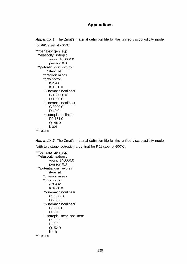
180
Appendices
Appendix 1. The Zmat’s material definition file for the unified viscoplasticity model
for P91 steel at 400˚C.
***behavior gen_evp **elasticity isotropic young 185000.0 poisson 0.3 **potential gen_evp ev *store_all *criterion mises *flow norton n 2.48 K 1250.0 *kinematic nonlinear C 183000.0 D 1000.0 *kinematic nonlinear C 8000.0 D 40.0 *isotropic nonlinear R0 151.0 Q -45.0 b 0.4 ***return Appendix 2. The Zmat’s material definition file for the unified viscoplasticity model
(with two stage isotropic hardening) for P91 steel at 600˚C.
***behavior gen_evp **elasticity isotropic young 140000.0 poisson 0.3 **potential gen_evp ev *store_all *criterion mises *flow norton n 3.482 K 1000.0 *kinematic nonlinear C 63000.0 D 900.0 *kinematic nonlinear C 5000.0 D 50.0 *isotropic linear_nonlinear R0 90.0 H -2.9 Q -52.0 b 1.9 ***return
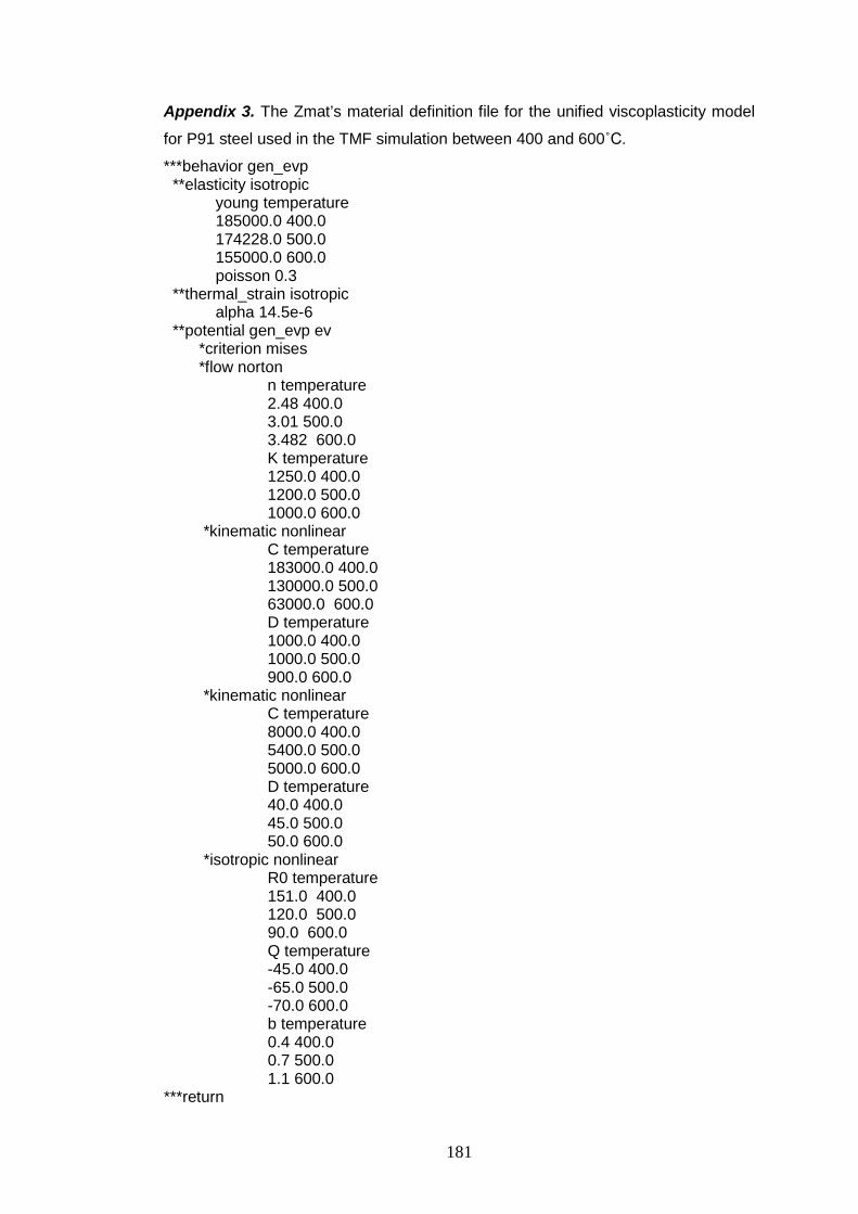
181
Appendix 3. The Zmat’s material definition file for the unified viscoplasticity model
for P91 steel used in the TMF simulation between 400 and 600˚C.
***behavior gen_evp **elasticity isotropic young temperature 185000.0 400.0 174228.0 500.0 155000.0 600.0 poisson 0.3 **thermal_strain isotropic alpha 14.5e-6 **potential gen_evp ev *criterion mises *flow norton n temperature 2.48 400.0 3.01 500.0 3.482 600.0 K temperature 1250.0 400.0 1200.0 500.0 1000.0 600.0 *kinematic nonlinear C temperature 183000.0 400.0 130000.0 500.0 63000.0 600.0 D temperature 1000.0 400.0 1000.0 500.0 900.0 600.0 *kinematic nonlinear C temperature 8000.0 400.0 5400.0 500.0 5000.0 600.0 D temperature 40.0 400.0 45.0 500.0 50.0 600.0 *isotropic nonlinear R0 temperature 151.0 400.0 120.0 500.0 90.0 600.0 Q temperature -45.0 400.0 -65.0 500.0 -70.0 600.0 b temperature 0.4 400.0 0.7 500.0 1.1 600.0 ***return


![Important Fatwas Regarding The Rites of Hajj and Umrah...dictated by Shaykh 'Abdul 'Aziz bin 'Abdullah bin Baz [rahimahullah]](https://img.pdfslide.us/doc/110x75/577d2c3c1a28ab4e1eabae30/important-fatwas-regarding-the-rites-of-hajj-and-umrahdictated-by-shaykh.jpg)