Embed Size (px)
Citation preview

PREPARATION AND OPERATIONS OF THE MISSION PERFORMANCE
CENTRE (MPC) FOR THE COPERNICUS SENTINEL-3 MISSION
S3-A MWR Cyclic Performance Report
Cycle No. 026
Start date: 20/12/2017
End date: 16/01/2018
Ref.: S3MPC.CLS.PR.05-026
Issue: 1.0
Date: 16/02/2018
Contract: 4000111836/14/I-LG

Customer: ESA Document Ref.: S3MPC.CLS.PR.05-026
Contract No.: 4000111836/14/I-LG Date: 16/02/2018
Issue: 1.0
Project: PREPARATION AND OPERATIONS OF THE MISSION PERFORMANCE CENTRE (MPC)
FOR THE COPERNICUS SENTINEL-3 MISSION
Title: S3-A MWR Cyclic Performance Report
Author(s): MWR ESLs
Approved by: G. Quartly, STM ESL
Coordinator
Authorized by Sylvie Labroue, STM Technical
Performance Manager
Distribution: ESA, EUMETSAT, S3MPC consortium
Accepted by ESA P. Féménias, MPC TO
Filename S3MPC.CLS.PR.05-026 - i1r0 - MWR Cyclic Report 026.docx
Disclaimer
The work performed in the frame of this contract is carried out with funding by the European Union. The views expressed herein can in no way be taken to reflect the official opinion of either the European Union or the
European Space Agency.
Sentinel-3 MPC
S3-A MWR Cyclic Performance Report
Cycle No. 026
Ref.: S3MPC.CLS.PR.05-026
Issue: 1.0
Date: 16/02/2018
Page: iii
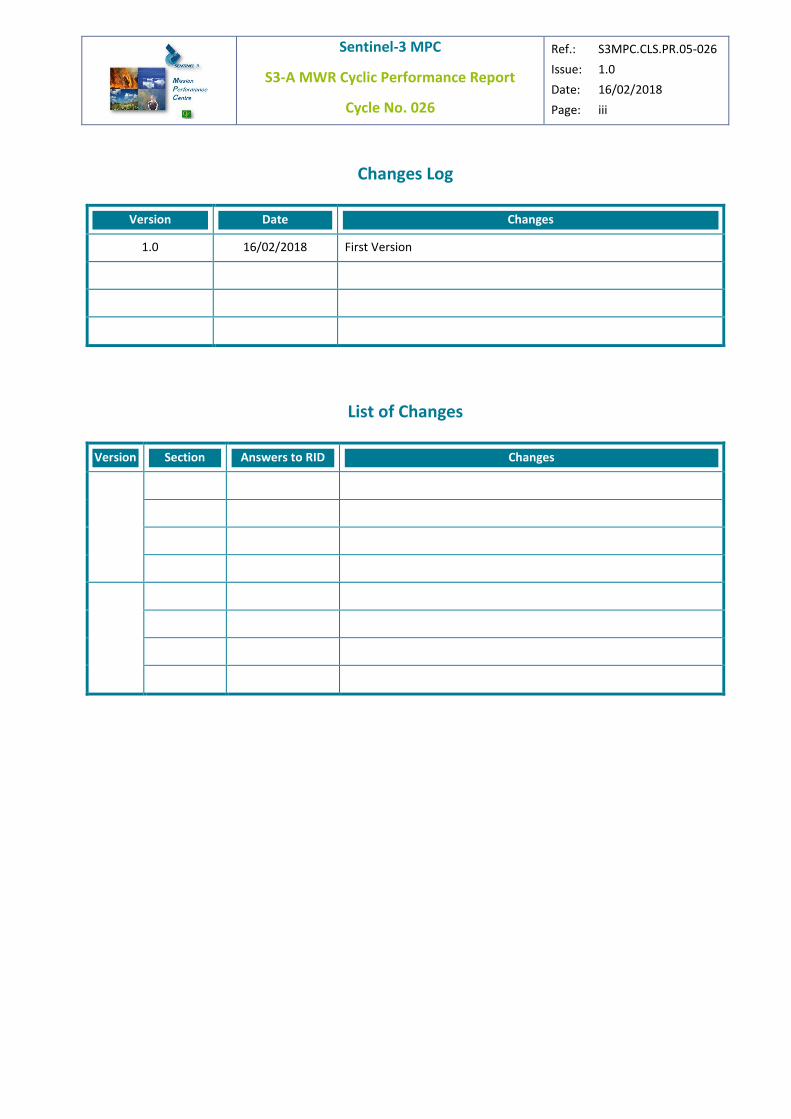
Changes Log
Version Date Changes
1.0 16/02/2018 First Version
List of Changes
Version Section Answers to RID Changes
Sentinel-3 MPC
S3-A MWR Cyclic Performance Report
Cycle No. 026
Ref.: S3MPC.CLS.PR.05-026
Issue: 1.0
Date: 16/02/2018
Page: iv
Table of content
1 INTRODUCTION ............................................................................................................................................ 1
2 OVERVIEW OF CYCLE 026 .............................................................................................................................. 2
2.1 STATUS ........................................................................................................................................................... 2
2.2 IPF PROCESSING CHAIN STATUS ........................................................................................................................... 3
2.2.1 IPF version ............................................................................................................................................... 3
2.2.2 Auxiliary Data files .................................................................................................................................. 4
3 MWR MONITORING OVER CYCLE 026 ........................................................................................................... 5
3.1 OPERATING MODES ........................................................................................................................................... 5
3.2 CALIBRATION PARAMETERS ................................................................................................................................. 6
3.2.1 Gain ......................................................................................................................................................... 6
3.2.2 Noise Injection Temperature ................................................................................................................... 7
3.3 BRIGHTNESS TEMPERATURES .............................................................................................................................. 7
3.4 GEOPHYSICAL PRODUCTS MONITORING ................................................................................................................. 9
3.4.1 Wet Tropospheric Correction .................................................................................................................. 9
3.4.2 Atmospheric Attenuation ...................................................................................................................... 11
4 LONG-TERM MONITORING ..........................................................................................................................12
4.1 INTERNAL CALIBRATION PARAMETERS ................................................................................................................. 12
4.1.1 Gain ....................................................................................................................................................... 12
4.1.2 Noise Injection temperature .................................................................................................................. 13
4.2 VICARIOUS CALIBRATION .................................................................................................................................. 14
4.2.1 Coldest ocean temperatures ................................................................................................................. 14
4.2.2 Amazon forest ....................................................................................................................................... 16
4.2.3 References ............................................................................................................................................. 18
4.3 GEOPHYSICAL PRODUCTS .................................................................................................................................. 18
4.3.1 Monitoring of geophysical products ...................................................................................................... 18
4.3.2 Comparison to in-situ measurements ................................................................................................... 22
5 SPECIFIC INVESTIGATIONS ...........................................................................................................................23

Sentinel-3 MPC
S3-A MWR Cyclic Performance Report
Cycle No. 026
Ref.: S3MPC.CLS.PR.05-026
Issue: 1.0
Date: 16/02/2018
Page: v
6 EVENTS ........................................................................................................................................................24
7 APPENDIX A .................................................................................................................................................25

Sentinel-3 MPC
S3-A MWR Cyclic Performance Report
Cycle No. 026
Ref.: S3MPC.CLS.PR.05-026
Issue: 1.0
Date: 16/02/2018
Page: vi
List of Figures
Figure 1 : Distribution of operating mode ---------------------------------------------------------------------------------- 5
Figure 2 : Map of measurements with DNB processing for 36.5GHz channel (red) and safety mode for
both channels over KREMS (blue) -------------------------------------------------------------------------------------------- 6
Figure 3 : Monitoring of receiver gain for both channels :23.8GHz (left) and 36.5GHz (right) ---------------- 7
Figure 4 : Monitoring of Noise Injection temperature for both channels :23.8GHz (left) and 36.5GHz
(right) -------------------------------------------------------------------------------------------------------------------------------- 7
Figure 5 : Map of Brightness temperatures of channel 23.8GHz for ascending (right) and descending
(left) passes ------------------------------------------------------------------------------------------------------------------------ 8
Figure 6 : Map of Brightness temperatures of channel 36.5GHz for ascending (right) and descending
(left) passes ------------------------------------------------------------------------------------------------------------------------ 8
Figure 7: Histograms of MWR-ECMWF difference of wet tropospheric correction for SARAL/MWR ,
Jason3/AMR and Sentinel-3A/MWR SAR and PLRM (selection of latitude between -60°/60° for all
instruments) ----------------------------------------------------------------------------------------------------------------------10
Figure 8 : MWR-ECMWF difference of wet tropospheric correction : using SAR (left) and PLRM altimeter
backscatter (right) ---------------------------------------------------------------------------------------------------------------10
Figure 9 : Jason3/AMR MWR-ECMWF difference of wet tropospheric correction (IGDR product) ---------10
Figure 10 : Ku band Atmospheric attenuation of the Sigma0 Left : Histograms for Sentinel-3A/MWR,
Jason3/AMR, Model attenuation; Right: Map of difference of MWR-model atmospheric attenuation for
Sentinel-3A ------------------------------------------------------------------------------------------------------------------------11
Figure 11 : Daily mean of the gain for both channels : 23.8GHz (left) and 36.5GHz (right) -------------------12
Figure 12 : Daily statistics of the noise injection temperature for channel 23.8GHz (left) and 36.5GHz
(right): mean (bold line), min/max (thin line), standard deviation (shade) ---------------------------------------13
Figure 13 : Coldest temperature over ocean at 23.8GHz for Sentinel-3A, SARAL/AltiKa, Jason2, Jason3
and Metop-A/AMSU-A ---------------------------------------------------------------------------------------------------------15
Figure 14 : Coldest temperature over ocean for the liquid water channel Sentinel-3A, SARAL/AltiKa,
Jason2, Jason3 and Metop-A/AMSU-A -------------------------------------------------------------------------------------16
Figure 15 : Average temperature over Amazon forest at 23.8GHz channel for Sentinel-3A, SARAL/AltiKa,
Jason2, Jason3, and Metop-A/AMSU-A ------------------------------------------------------------------------------------17
Sentinel-3 MPC
S3-A MWR Cyclic Performance Report
Cycle No. 026
Ref.: S3MPC.CLS.PR.05-026
Issue: 1.0
Date: 16/02/2018
Page: vii
Figure 16 : Average temperature over Amazon forest at 36.5GHz channel for Sentinel-3A, SARAL/AltiKa,
Jason2, Jason3 and Metop-A/AMSU-A -------------------------------------------------------------------------------------17
Figure 17 : Monitoring of difference MWR-model wet tropo. correction: daily average (left) and standard
deviation (right). Selection of points with latitude between -60° and 60° ----------------------------------------19
Figure 18 : Monitoring of difference MWR-model atmospheric attenuation: daily average (left) and
standard deviation (right). Selection of points with latitude between -60° and 60° ----------------------------20
Figure 19 : Monitoring of difference MWR-ECMWF water vapour content: daily average (left) and
standard deviation (right). Selection of points with latitude between -60° and 60° ----------------------------21
Figure 20 : Monitoring of difference MWR-ECMWF cloud liquid water content: daily average (left) and
standard deviation (right). Selection of points with latitude between -60° and 60° ----------------------------21
List of Tables
Table 1 : General overview of the MWR quality assessment ---------------------------------------------------------- 2

Sentinel-3 MPC
S3-A MWR Cyclic Performance Report
Cycle No. 026
Ref.: S3MPC.CLS.PR.05-026
Issue: 1.0
Date: 16/02/2018
Page: 1
1 Introduction
This document aims at providing a synthetic report on the behaviour of the radiometer in terms of
instrumental characteristics and product performances as well as on the main events which occurred
during cycle 26.
This document is split in the following sections:
Section 2 gives an overview on the status of the current cycle
Section 3 addresses the monitoring of the MWR of the current cycle. This section covers the
short term monitoring of internal calibration, brightness temperatures and geophysical
parameters.
Section 4 addresses the long term monitoring from the beginning of the mission. It provides a
view of the internal calibration monitoring as well as two subsections covering the monitoring of
vicarious calibration targets and geophysical parameters.
Sentinel-3 MPC
S3-A MWR Cyclic Performance Report
Cycle No. 026
Ref.: S3MPC.CLS.PR.05-026
Issue: 1.0
Date: 16/02/2018
Page: 2
2 Overview of Cycle 026
2.1 Status
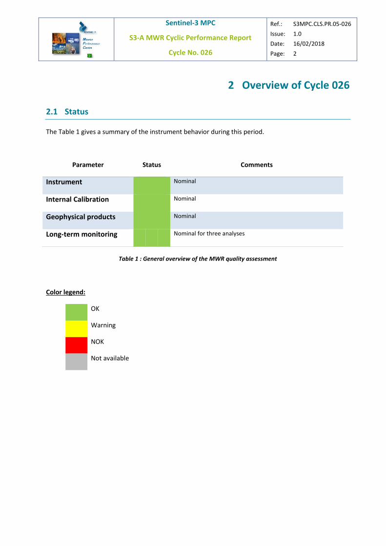
The Table 1 gives a summary of the instrument behavior during this period.
Parameter Status Comments
Instrument Nominal
Internal Calibration Nominal
Geophysical products Nominal
Long-term monitoring Nominal for three analyses
Table 1 : General overview of the MWR quality assessment
Color legend:
OK
Warning
NOK
Not available

Sentinel-3 MPC
S3-A MWR Cyclic Performance Report
Cycle No. 026
Ref.: S3MPC.CLS.PR.05-026
Issue: 1.0
Date: 16/02/2018
Page: 3
2.2 IPF processing chain status
2.2.1 IPF version
This section gives the version of the IPF processing chain used to process the data of the current cycle.
If a change of IPF version occurs during the cycle, the table gives the date of last processing with the first
version and the date of first processing with the second version:
: first date of processing
: last date of processing
MWR L1B CAL
IPF version NRT from Svalbard
06.04
MWR L1B
IPF version NTC ( LN3)
06.04
SRAL/MWR Level 2
IPF version NTC ( LN3)
06.10
Sentinel-3 MPC
S3-A MWR Cyclic Performance Report
Cycle No. 026
Ref.: S3MPC.CLS.PR.05-026
Issue: 1.0
Date: 16/02/2018
Page: 4
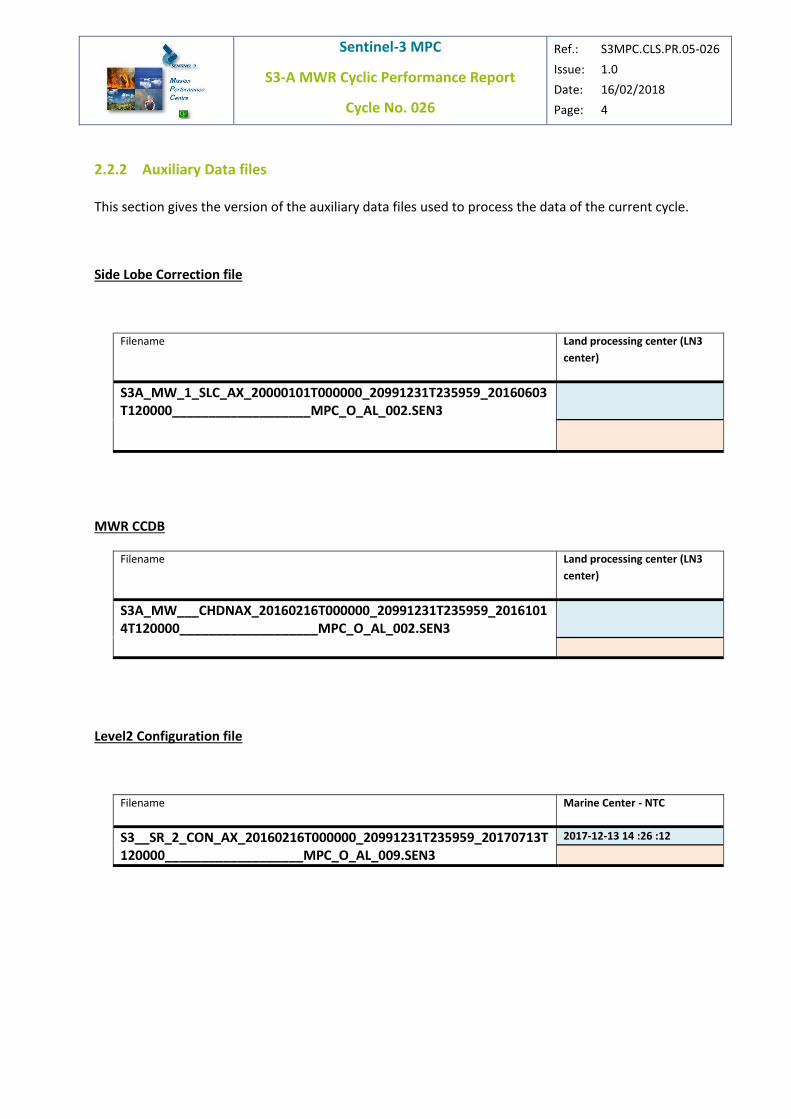
2.2.2 Auxiliary Data files
This section gives the version of the auxiliary data files used to process the data of the current cycle.
Side Lobe Correction file
Filename Land processing center (LN3
center)
S3A_MW_1_SLC_AX_20000101T000000_20991231T235959_20160603T120000___________________MPC_O_AL_002.SEN3
MWR CCDB
Filename Land processing center (LN3
center)
S3A_MW___CHDNAX_20160216T000000_20991231T235959_20161014T120000___________________MPC_O_AL_002.SEN3
Level2 Configuration file
Filename Marine Center - NTC
S3__SR_2_CON_AX_20160216T000000_20991231T235959_20170713T120000___________________MPC_O_AL_009.SEN3
2017-12-13 14 :26 :12

Sentinel-3 MPC
S3-A MWR Cyclic Performance Report
Cycle No. 026
Ref.: S3MPC.CLS.PR.05-026
Issue: 1.0
Date: 16/02/2018
Page: 5
3 MWR Monitoring over Cycle 026
This section is dedicated to the functional verification of the MWR sensor behaviour during cycle 26 (20
December 2017 – 16 January 2018) . The main relevant of the parameters, monitored daily by the MPC
team, are presented here.
3.1 Operating modes
The radiometer has several operating modes listed hereafter:
Mode 0 : Intermonitoring (Earth observation)
Mode 1 : Monitoring
Mode 2 : Noise Injection calibration
Mode 3 : Dicke Non-Balanced calibration (100% injection – hot point)
Mode 4 : Dicke Non-Balanced calibration (50% injection – cold point)
Figure 1 gives the distribution of the different modes in the data.
Figure 1 : Distribution of operating mode
For measurements in the Intermonitoring mode, two kind of processing can be used according to the
measured brightness temperature. If this temperature is smaller than the reference load inside the
instrument, the NIR processing is used; if the temperature is greater, the DNB processing is used. The
transition from one processing to the other will occur more or less close to the coast depending on the
internal temperature of the MWR. The internal temperature of the MWR is such that only a small
percentage of measurements required a DNB processing in this cycle as shown by Figure 2.

Sentinel-3 MPC
S3-A MWR Cyclic Performance Report
Cycle No. 026
Ref.: S3MPC.CLS.PR.05-026
Issue: 1.0
Date: 16/02/2018
Page: 6
This figure shows also the passage over the US KREMS radar facility in the Kwajalein atoll (9°23’47’’ N -
167°28’50’’ E) in the Pacific. For safety reasons, the MWR is switched to a specific mode about 50 km
before the facility location and back to nominal mode 50km after.
Figure 2 : Map of measurements with DNB processing for 36.5GHz channel (red) and safety mode for both
channels over KREMS (blue)
3.2 Calibration parameters
To monitor the instrument behavior during its lifetime, the relevant parameters of the MWR internal in-
flight calibration procedure are presented in the following subsections. These parameters are:
the gain : this parameter is estimated using the two types of Dicke Non-Balanced calibration
measurements (100% and 50% of injection). The DNB processing of the Earth measurements
uses this parameter.
the noise injection temperature: this parameter is measured during the Noise Injection
calibration measurements. The NIR processing of the Earth measurements uses this parameter.
Data used for the diagnosis presented here are data generated by PDGS at Svalbard core ground station.
3.2.1 Gain
Figure 3 shows the monitoring of the receiver gain for the current cycle. The mean value over the cycle
is 4.76mv/K and 4.53mV/K for channel 23.8GHz and 36.5GHz respectively. These values are close to
values estimated on-ground during characterization of the instrument (4.793mV/K and 4.665mV/K for
channels 23.8GHz and 36.5GHz respectively). For channel 23.8GHz, the estimated receiver gain show no
trend during this cycle. For the second channel, a small decrease of about 0.005mV/K is observed over
the cycle. Nominal behavior is observed since only 1 cycle of data is considered in this section.

Sentinel-3 MPC
S3-A MWR Cyclic Performance Report
Cycle No. 026
Ref.: S3MPC.CLS.PR.05-026
Issue: 1.0
Date: 16/02/2018
Page: 7
Figure 3 : Monitoring of receiver gain for both channels :23.8GHz (left) and 36.5GHz (right)
3.2.2 Noise Injection Temperature
Figure 4 shows the monitoring of the noise injection temperature for the current cycle. The noise
injection temperature is constant over the cycle for channel 23.8GHz close to 313.9K. A very small
decrease is observed (less than 0.1K in average) for 36.5GHz channel starting from 288K. Nominal
behavior is observed since only 1 cycle of data is considered in this section.
Figure 4 : Monitoring of Noise Injection temperature for both channels :23.8GHz (left) and 36.5GHz (right)
3.3 Brightness Temperatures
Data used for the diagnosis presented here are data generated at Land Surface Topography Mission
Processing and Archiving Centre [LN3].
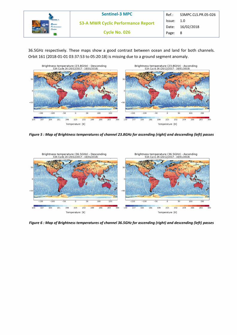
The two following figures show maps of brightness temperatures for both channels split by ascending
(right part) and descending (left part) passes. Figure 5 and Figure 6 concern the channels 23.8GHz and
Sentinel-3 MPC
S3-A MWR Cyclic Performance Report
Cycle No. 026
Ref.: S3MPC.CLS.PR.05-026
Issue: 1.0
Date: 16/02/2018
Page: 8
36.5GHz respectively. These maps show a good contrast between ocean and land for both channels.
Orbit 161 (2018-01-01 03:37:53 to 05:20:18) is missing due to a ground segment anomaly.
Figure 5 : Map of Brightness temperatures of channel 23.8GHz for ascending (right) and descending (left) passes
Figure 6 : Map of Brightness temperatures of channel 36.5GHz for ascending (right) and descending (left) passes

Sentinel-3 MPC
S3-A MWR Cyclic Performance Report
Cycle No. 026
Ref.: S3MPC.CLS.PR.05-026
Issue: 1.0
Date: 16/02/2018
Page: 9
3.4 Geophysical products monitoring
The inversion algorithms allow to retrieve the geophysical products from the measurements of the
radiometer (brightness temperatures measured at two different frequencies) and the altimeter
(backscattering coefficient ie sigma0). Four geophysical products are issued from the retrieval
algorithms: the wet tropospheric correction, the atmospheric attenuation of the Sigma0, the water
vapor content, the cloud liquid water content. This section provides an assessment of two of these
retrievals used by the SRAL/MWR L2 processing: the wet tropospheric correction and the atmospheric
attenuation of the Sigma0. The wet tropospheric correction is analysed through the MWR-ECMWF
difference of this correction.
3.4.1 Wet Tropospheric Correction
Figure 7 presents the histograms of the MWR-ECMWF differences of wet tropospheric correction
(ΔWTC) for cycle 26. In this figure, Sentinel-3A/MWR correction is compared to the correction retrieved
by Jason-3/AMR (IGDR) and SARAL/MWR (IGDR) over the same period.
The standard deviation of the difference MWR-ECMWF corrections for S-3A is around 1.40cm and
1.39cm for SAR and PLRM corrections respectively while it is 1.57cm for SARAL and 1.21cm for Jason-3.
First Jason-3 benefits from its three channels radiometer (18.7GHz, 23.8GHz, 34GHz), providing a
correction with a smaller deviation with respect to the model. SARAL/MWR is closer to S-3A/MWR in
this context with its two channels (23.8GHZ and 37GHz for SARAL, 23.8 and 36.5GHz for S-3A). Then the
standard deviation for SARAL is the closest reference, even though the Sigma0 in Ka band raises some
questions. With the use of STC products for S-3A, the ΔWTC for the three instruments are directly
comparable since all use ECMWF analyses for the computation of the model correction. The standard
deviation of ΔWTC for S-3A is smaller than for SARAL meaning that we have a better estimation of the
correction for S-3A according to these metrics. Jason-3 gives the best performances with the smallest
deviation. Moreover, one can notice that both SAR and PLMR corrections have very similar
performances: mean(std) of ΔWTC being close to 0.15cm(1.40cm) and 0.16cm(1.39cm) for SAR and
PLRM respectively.
Figure 8 presents a map of the ΔWTC for Sentinel-3A only for SAR correction on the left and PLRM
correction on the right. For this cycle, the maps show geographical patterns expected for this
parameter. Note that the color scale is centered to the mean value. The comparison with Jason2 map of
ΔWTC (Figure 9) shows similarities although Sentinel-3A ΔWTC is larger than Jason2 because of their
different instrument configuration.

Sentinel-3 MPC
S3-A MWR Cyclic Performance Report
Cycle No. 026
Ref.: S3MPC.CLS.PR.05-026
Issue: 1.0
Date: 16/02/2018
Page: 10
Figure 7: Histograms of MWR-ECMWF difference of wet tropospheric correction for SARAL/MWR , Jason3/AMR
and Sentinel-3A/MWR SAR and PLRM (selection of latitude between -60°/60° for all instruments)
Figure 8 : MWR-ECMWF difference of wet tropospheric correction : using SAR (left) and PLRM altimeter
backscatter (right)
Figure 9 : Jason3/AMR MWR-ECMWF difference of wet tropospheric correction (IGDR product)

Sentinel-3 MPC
S3-A MWR Cyclic Performance Report
Cycle No. 026
Ref.: S3MPC.CLS.PR.05-026
Issue: 1.0
Date: 16/02/2018
Page: 11
3.4.2 Atmospheric Attenuation
The left part of Figure 10 presents the histograms of the Ku band atmospheric attenuation of the
Sigma0. In this figure, Sentinel-3A attenuation is compared to the model attenuation computed from
ECMWF analyses and Jason3 attenuation from IGDR products. The results for both instruments are very
similar to model results with an average attenuation close to 0.21dB for S-3A , 0.19dB for Jason3 and
0.2dB for model attenuation. Note that the model attenuation shows in that histogram is the
attenuation computed at Sentinel-3A time and geolocation. The right panel of Figure 10 shows a map of
the difference of MWR attenuation and model attenuation computed from ECMWF analyses for
Sentinel-3A. Globally a bias of 0.01 dB between MWR and model attenuation can be estimated from this
plot.
Figure 10 : Ku band Atmospheric attenuation of the Sigma0
Left : Histograms for Sentinel-3A/MWR, Jason3/AMR, Model attenuation; Right: Map of difference of MWR-
model atmospheric attenuation for Sentinel-3A

Sentinel-3 MPC
S3-A MWR Cyclic Performance Report
Cycle No. 026
Ref.: S3MPC.CLS.PR.05-026
Issue: 1.0
Date: 16/02/2018
Page: 12
4 Long-term monitoring
In this section, a long-term monitoring of the MWR behaviour is presented.
4.1 Internal Calibration parameters
This section presents a long-term monitoring of internal calibration parameters. Data used for the
diagnosis presented here are:
Reprocessed data (processing baseline 2.15) from cycle 1 to cycle 16
MWR L1B data generated by PDGS at Svalbard core ground station are used from 26/10/2016
4.1.1 Gain
Figure 11 shows the daily mean of the receiver gain for both channels. This calibration parameter is used
in the DNB processing of the measurements. As seen previously in section 3.1, only a small part of the
measurements are processed in DNB mode. The first part of the monitoring of the calibration
parameters shown here is performed with products generated during the reprocessing of processing
baseline 2.15, the second part using NRT products from the day of the IPF update on the Svalbard
ground station forward.
From the two panels of Figure 11, one can see that the receiver gain has a different evolution for each
channel. The gain for the 23.8GHz channel has slowly increased since the beginning of the mission
showing four slopes and three inflexion points at August 2016, Februray 2017 and June 2017. It seems
to be almost stable since cycle 19 (July 2017). The gain has increased of +0.03mv/K since the beginning
of the mission. For the 36.5GHz channel, the gain is increasing from cycle 1 and then starts to decrease
at the beginning of cycle 4. During cycle 15, it started to increase again until cycle 18 and then starts a
decrease. The gain has decreased of 0.03mV/K since the beginning of the mission. Due to the small
number of data processed using this parameter, it will be difficult to assess if this decrease has an
impact on data quality. The monitoring will be pursued and data checked for any impact.
Figure 11 : Daily mean of the gain for both channels : 23.8GHz (left) and 36.5GHz (right)

Sentinel-3 MPC
S3-A MWR Cyclic Performance Report
Cycle No. 026
Ref.: S3MPC.CLS.PR.05-026
Issue: 1.0
Date: 16/02/2018
Page: 13
4.1.2 Noise Injection temperature
Figure 12 shows the daily mean of the noise injection temperature for both channels. This calibration
parameter is used in the NIR processing of the measurements. As seen previously in section 3.1, the
main part of the measurements are processed in NIR mode. Moreover the first part of the monitoring of
the calibration parameters is performed using products generated during the reprocessing os processing
baseline 2.15, the second part using NRT calibration products from the day of the IPF update on the
ground station.
From the two panels of Figure 12, one can see that the noise injection parameter has a different
evolution for each channel. For the 23.8GHz channel, the noise injection temperature has decreased of
less than 0.5K during the first 2 cycles, after what there has been no significant change of behaviour
until cycle 13. During this cycle, the noise injection temperature seems to start a slow decrease. For the
channel 36.5GHz, one can see that the injection temperature is not stable : it seems to follow some kind
of periodic signal combined with a trend. Since cycle 19, the gain is slowly decreasing as it has done from
July2016 to February 2017. The monitoring will be pursued and data checked for any impact.
Some peak values are noticeable at the end of cycle 4 (mainly channel 23.8GHz), at the end of cycle 6,
during cycle 9, 10, 12 and 16. Some of these peaks concerns both channels at the same time, while a
small part of them only one of them. The investigations performed in the cycle 6 report has shown that
these measurements are localized around a band of latitude that may change along the time series. The
source is not yet clearly identified but a intrusion of the Moon in the sky horn is suspected.
Figure 12 : Daily statistics of the noise injection temperature for channel 23.8GHz (left) and 36.5GHz (right):
mean (bold line), min/max (thin line), standard deviation (shade)

Sentinel-3 MPC
S3-A MWR Cyclic Performance Report
Cycle No. 026
Ref.: S3MPC.CLS.PR.05-026
Issue: 1.0
Date: 16/02/2018
Page: 14
4.2 Vicarious calibration
The assessment of the brightness temperatures quality and stability is performed using vicarious
calibrations. Two specific areas are selected. Sentinel-3A data used in this section are:
Coldest ocean temperature analysis uses Level 2 data
data from processing baseline 2.15 reprocessing from June 2016 to April 2017.
STC Marine data from December 2016 to December 2017
NTC Marine data since cycle 26
Amazon forest analysis uses Level 1B data:
data from processing baseline 2.15 reprocessing from June 2016 to April 2017.
STC Land data from LN3 processing center
NTC Marine data since cycle 26
4.2.1 Coldest ocean temperatures
The first area is the ocean and more precisely the coldest temperature over ocean. Following the
method proposed by Ruf [RD 1], updated by Eymar [RD 3] and implemented in [RD 7], the coldest ocean
temperatures is computed by a statistic selection. Ruf has demonstrated how a statistical selection of
the coldest BT over ocean allows detecting and monitoring drifts. It is also commonly used for long-term
monitoring or cross-calibration [RD 4] [RD 5] [RD 6].
The Figure 13 presents the coldest ocean temperature computed following method previously described
at 23.8GHz channel for Sentinel-3A/WMR and three other microwave radiometers: AltiKa/MWR,
Jason2/Jason3/AMR and Metop-A/AMSU-A. For AMSU-A, the two pixels of smallest incidence (closest to
nadir) are averaged. The Figure 14 presents the same results for the liquid water channel of the same
four instruments: 36.5GHz for Sentinel-3A, 37GHz for AltiKa , 34GHz for Jason2/Jason3 and 31.4GHz for
Metop-A.
Concerning the 23.8GHz channel presented on Figure 12, one can see the impact of the calibration of
the MWR with the increase of the coldest ocean brightness temperature: around 135K before and 140K
after the update of the characterisation file and LTM files for the STC on the fly products (green line).
The temperature of the coldest ocean points is now closer to the other sun-synchroneous missions
(Metop-A, SARAL/AltiKa). The light green line is for the reprocessed data of processing baseline 2.15
that is with the same configuration than the on-the-fly products after January. One can notice the very
good agreement on the overlaping period.

Sentinel-3 MPC
S3-A MWR Cyclic Performance Report
Cycle No. 026
Ref.: S3MPC.CLS.PR.05-026
Issue: 1.0
Date: 16/02/2018
Page: 15
The analysis for the liquid water channel (Figure 14) is more complicated due to the different frequency
used by these instruments for this channel: 36.5GHz for Sentinel-3A, 37GHz for AltiKa, 34GHz for
Jason2/Jason3 and 31.4Ghz for AMSU-A. But the coldest temperature can be used relatively one with
another. For instance, one can see that the difference between AltiKa and Jason-2/Jason3 is about 6K
which is in line with the theoretical value estimated by Brown between the channel 34 GHz of JMR and
the channel 37 GHz of TMR (-5.61 K ± 0.23 K) [RD 8]. Then we can expect that Sentinel3 should be closer
to AltiKa than Jason2 due to the measurement frequency. The STC and NTC products reprocessed using
the new MWR characterisation file (light green curves) show hottest temperatures like AltiKa. For the
on-the-fly STC products, a jump in the temperatures occurs with the update of MWR characterisation
file.
The period is too short to allow a drift analysis but it is reassuring to see that Sentinel-3A/MWR has the
same behaviour than the other radiometer.
Figure 13 : Coldest temperature over ocean at 23.8GHz for Sentinel-3A, SARAL/AltiKa, Jason2, Jason3 and
Metop-A/AMSU-A

Sentinel-3 MPC
S3-A MWR Cyclic Performance Report
Cycle No. 026
Ref.: S3MPC.CLS.PR.05-026
Issue: 1.0
Date: 16/02/2018
Page: 16
Figure 14 : Coldest temperature over ocean for the liquid water channel Sentinel-3A, SARAL/AltiKa, Jason2,
Jason3 and Metop-A/AMSU-A
4.2.2 Amazon forest
The second area is the Amazon forest which is the natural body the closest to a black body for
microwave radiometry. Thus it is commonly used to assess the calibration of microwave radiometers
[RD 2][ RD 3]. The method proposed in these papers have been used as a baseline to propose a new
method implemented in [RD 7]. In this new approach, a mask is derived from the evergreen forest class
of GlobCover classification over Amazon. The average temperature is computed here over a period of
one month for all missions.
The averaged temperature over the Amazon forest is shown on Figure 15 and Figure 16 for water vapor
channel (23.8GHz) and liquid water channel respectively. These two figures show the very good
consistency of Sentinel-3A with the three other radiometers on the hottest temperatures: around 286K
for the first channel, and 284K for the second channel. The mean value as well as the annual cycle is well
respected. These results show the correct calibration for the hottest temperatures and the small impact
of the MWR calibration for the hottest temperatures when comparing the reprocessed data using
processing baseline 2.15 (light green line) and the on-the-fly products, here STC L1B products . As for the
coldest ocean temperatures, the period is too short to allow a drift analysis.

Sentinel-3 MPC
S3-A MWR Cyclic Performance Report
Cycle No. 026
Ref.: S3MPC.CLS.PR.05-026
Issue: 1.0
Date: 16/02/2018
Page: 17
Figure 15 : Average temperature over Amazon forest at 23.8GHz channel for Sentinel-3A, SARAL/AltiKa, Jason2,
Jason3, and Metop-A/AMSU-A
Figure 16 : Average temperature over Amazon forest at 36.5GHz channel for Sentinel-3A, SARAL/AltiKa, Jason2,
Jason3 and Metop-A/AMSU-A
Sentinel-3 MPC
S3-A MWR Cyclic Performance Report
Cycle No. 026
Ref.: S3MPC.CLS.PR.05-026
Issue: 1.0
Date: 16/02/2018
Page: 18
4.2.3 References
RD 1 C. Ruf, 2000: Detection of Calibration Drifts in spaceborne Microwave Radiometers using a Vicarious cold
reference, IEEE Trans. Geosci. Remote Sens., 38, 44-52
RD 2 S. Brown, C. Ruf, 2005: Determination of an Amazon Hot Reference Target for the on-orbit calibration of
Microwave radiometers, Journal of Atmos. Ocean. Techno., 22, 1340-1352
RD 3 L. Eymard, E. Obligis, N. Tran, F. Karbou, M. Dedieu, 2005: Long term stability of ERS-2 and TOPEX microwave
radiometer in-flight calibration, IEEE Trans. Geosci. Remote Sens., 43, 1144-1158
RD 4 C. Ruf, 2002: Characterization and correction of a drift in calibration of the TOPEX microwave radiometer,
IEEE Trans. Geosci. Remote Sens., 40, 509-511
RD 5 R. Scharoo, J. Lillibridge, W. Smith, 2004: Cross-calibration and long-term monitoring of the microwave
radiometers of ERS, TOPEX, GFO, Jason and Envisat, Marine Geodesy, 27, 279-297
RD 6 R. Kroodsma, D. McKague, C. Ruf, 2012: Inter-Calibration of Microwave Radiometers Using the Vicarious Cold
Calibration Double Difference Method, Applied Earth Obs. and Remote Sensing, 5, 1939-1404
RD 7 Estimation des dérives et des incertitudes associées pour les radiomètres micro-ondes. Revue des méthodes
existantes, SALP-NT-MM-EE-22288,
RD 8 Brown, S., C. Ruf, S. Keihm, and A. Kitiyakara, “Jason Microwave Radiometer Performance and On-Orbit
Calibration,” Mar. Geod., vol. 27, no. 1–2, pp. 199–220, 2004.
4.3 Geophysical products
4.3.1 Monitoring of geophysical products
In this section, comparisons of MWR-model fields are performed for several instruments. The selected
instruments are Jason2/Jason3/AMR and SARAL/AltiKa. For a long-term monitoring perspective, GDR
products are used to compute the difference with respect to model values. Model values for each field
are computed using ECMWF analyses data. GDR products for each mission have their own latency due
to cycle curation and mission constraints such as the cold-sky calibration for Jason2 and Jason3 missions.
Indeed, AltiKa GDR is available with delay of 35 days, while for Jason2 or Jason3 this delay is up to 60
days.
4.3.1.1 Wet tropospheric correction
Figure 17 shows the monitoring of the MWR-model differences of wet tropospheric correction (ΔWTC)
using Level2 STC products from the Marine Center. Sentinel-3A correction is compared to Jason2/AMR,
Jason3/AMR and SARAL/MWR corrections. For SARAL (annoted AL in Figure 17) , Jason2 (J2) and Jason3
(J3), GDR products were selected. The daily average of ΔWTC for Sentinel-3A is close to 0cm since 10th of
January while it is around 0.6cm for SARAL and Jason2. This difference is small and results partialy from
the inversion algorithm.

Sentinel-3 MPC
S3-A MWR Cyclic Performance Report
Cycle No. 026
Ref.: S3MPC.CLS.PR.05-026
Issue: 1.0
Date: 16/02/2018
Page: 19
The more relevant parameter to assess the performance of a correction is the standard deviation of
ΔWTC. First Jason-2 and Jason3 benefit from their three channels radiometer (18.7GHz, 23.8GHz,
34GHz), providing a correction with a smaller deviation with respect to the model. SARAL/MWR is closer
to S-3A/MWR in this context with its two channels (23.8GHZ, 37GHz). Then the standard deviation for
SARAL is the closest reference, even though the Sigma0 in Ka band raises some questions. With the use
of STC products for S-3A, the ΔWTC for the three instruments are directly comparable since all missions
use ECMWF analyses for the computation of the model correction. The standard deviation of ΔWTC for
S-3A is smaller than for SARAL meaning that we have a better estimation of the correction for S-3A
according to these metrics. Jason2 and Jason3 give the best performances with the smallest deviation.
Moreover, one can notice that both SAR and PLMR corrections have very similar performances.
A change in the average ΔWTC evolution is observed in october 2017. After a slight increase since May
2017, a sudden decrease is observed in October followed by a sudden increase at the end of the same
month, also observed by AltiKa, while Jason3 data shows a small decrease. There is no software update
in that period that can explain this change of behaviour. From these results, the more relevant
hypothesis is that the change comes from the model. ΔWTC is constant since September 2017 for
Sentinel-3A and AltiKa.
Figure 17 : Monitoring of difference MWR-model wet tropo. correction: daily average (left) and standard
deviation (right). Selection of points with latitude between -60° and 60°
4.3.1.2 Atmospheric attenuation
Figure 18 shows the monitoring of the MWR-model differences of atmospheric attenuation (ΔATM_ATT)
using Level2 STC products from the Marine Center. Sentinel-3A correction in Ku band is compared to
Jason2/AMR andJason3/AMR. SARAL/AltiKa is not shown here because the altimeter uses the Ka band.
Figure 18 shows that the several evolutions affected mainly the average value of ΔATM_ATT: the daily
average show steps when the configuration of the IPF is updated, while the standard deviation remains
stable over the period. The mean of ΔATM_ATT for Jason2 and Jason-3 is 0.004dB and 0.003dB
respectively, a little larger for S-3A with 0.013dB. The evolution is stable for Jason2/3, some jumps are
observable for Sentinel-3A. The steps at the beginning of the period are due to processing configuration
changes (MWR characterisation file, Long Term Monitoring file). During cycle 25, a step is observed over

Sentinel-3 MPC
S3-A MWR Cyclic Performance Report
Cycle No. 026
Ref.: S3MPC.CLS.PR.05-026
Issue: 1.0
Date: 16/02/2018
Page: 20
the mean and standard deviation of the difference. This step corresponds to the IPF update which
corrected the coding of the atmospheric attenuation in the product. The atmospheric attenuation can
now have higher values in case of strong attenuation events. These points have an impact on the mean
and the standard deviation because they are very strong with respect to the average attenuation in Ku
band. A finer tuning of the retrieval algorithm is expected to correct for this small difference.
Figure 18 : Monitoring of difference MWR-model atmospheric attenuation: daily average (left) and standard
deviation (right). Selection of points with latitude between -60° and 60°
4.3.1.3 Water vapor content
Figure 19 shows the monitoring of the MWR-model differences of atmospheric attenuation (ΔWV) using
Level2 ShortTimeCritical (STC) and Non Time Critical (NTC) products from the Marine Center. Sentinel-
3A correction is compared to Jason2/AMR and Jason3/AMR. Figure 19 shows that the several evolutions
affected mainly the average value of ΔWV: the daily average show steps when the configuration of the
IPF is updated, while the standard deviation is stable over the whole period. The mean of ΔWV for
Jason2 is around -0.75kg/m2, very close to AltiKa results of -0.56kg/m2, around -1.08kg/m2 for Jason3,
and a little larger for Sentinel-3A: around 0.25kg/m2 in average. The standard deviation of ΔWV is very
similar between AltiKa (2.51kg/m2) and S-3A (2.25kg/m2 for PLRM), and a little smaller for Jason2 and
Jason3 around 2kg/m2. A finer tuning of the retrieval algorithm is expected to correct for the small
difference of the daily average.
A change in the average ΔWV evolution is observed in october 2017. After a slight decrease since May
2017, a sudden increase is observed in October followed by a sudden decrease at the end of the same
month, evolution also observed by AltiKa. Jason3 data show a small increase at the same period than
S3A and AltiKa but with a smaller amplitude. There is no software update in that period that can explain
this change of behaviour. From these results, it seems that the change comes from the model.

Sentinel-3 MPC
S3-A MWR Cyclic Performance Report
Cycle No. 026
Ref.: S3MPC.CLS.PR.05-026
Issue: 1.0
Date: 16/02/2018
Page: 21
Figure 19 : Monitoring of difference MWR-ECMWF water vapour content: daily average (left) and standard
deviation (right). Selection of points with latitude between -60° and 60°
4.3.1.4 Cloud liquid water content
Figure 20 shows the monitoring of the MWR-model differences of cloud liquid water content (ΔWC)
using Level2 STC products from the Marine Center. Sentinel-3A fields is compared to Jason2/AMR,
Jason3/AMR and SARAL/AltiKa. Figure 20 shows that the several evolutions affected mainly the average
value of ΔWC: the daily average show steps when the configuration of the IPF is updated but with a
smaller effect than for the other geophysical parameters, while the standard deviation is stable over the
whole period. The mean of ΔWC is close to 0.04kg/m2 for AltiKa, Jason2 and S-3A but around 0.02kg/m2
for Jason3. The standard deviation of Sentinel-3A is little higher than for the three other missions:
~0.3kg/m2 for S3-A, 0.2 kg/m2 for the other missions. This point needs to be analyzed.
As for the wet tropospheric correction and the water vapor content, a change in the average ΔWC
evolution is observed in october 2017. From the analysis performed for the other parameters, it seems
that the change comes from the model.
Figure 20 : Monitoring of difference MWR-ECMWF cloud liquid water content: daily average (left) and standard
deviation (right). Selection of points with latitude between -60° and 60°

Sentinel-3 MPC
S3-A MWR Cyclic Performance Report
Cycle No. 026
Ref.: S3MPC.CLS.PR.05-026
Issue: 1.0
Date: 16/02/2018
Page: 22
4.3.2 Comparison to in-situ measurements
The comparison of wet tropospheric correction to Radiosonde measurements will be addressed with 2
years of data.
Sentinel-3 MPC
S3-A MWR Cyclic Performance Report
Cycle No. 026
Ref.: S3MPC.CLS.PR.05-026
Issue: 1.0
Date: 16/02/2018
Page: 23
5 Specific investigations
None.

Sentinel-3 MPC
S3-A MWR Cyclic Performance Report
Cycle No. 026
Ref.: S3MPC.CLS.PR.05-026
Issue: 1.0
Date: 16/02/2018
Page: 24
6 Events
Add here the list of all MWR events happened during the cycle.

Sentinel-3 MPC
S3-A MWR Cyclic Performance Report
Cycle No. 026
Ref.: S3MPC.CLS.PR.05-026
Issue: 1.0
Date: 16/02/2018
Page: 25
7 Appendix A
Other reports related to the STM mission are:
S3-A SRAL Cyclic Performance Report, Cycle No. 026 (ref. S3MPC.ISR.PR.04-026)
S3-A Ocean Validation Cyclic Performance Report, Cycle No. 026 (ref. S3MPC.CLS.PR.06-026)
S3-A Winds and Waves Cyclic Performance Report, Cycle No. 026 (ref. S3MPC.ECM.PR.07-026)
S3-A Land and Sea Ice Cyclic Performance Report, Cycle No. 026 (ref. S3MPC.UCL.PR.08-026)
All Cyclic Performance Reports are available on MPC pages in Sentinel Online website, at:
https://sentinel.esa.int
End of document