Embed Size (px)
Citation preview

W h i t e P a P e r
S T R A T E G I C
A S S E T A L L O C A T I O N
March 2011
Issue #6
Karl EychenneResearch & DevelopmentLyxor Asset Management, [email protected]
Stéphane MartinettiResearch & DevelopmentLyxor Asset Management, [email protected]
Thierry RoncalliResearch & DevelopmentLyxor Asset Management, [email protected]


Q u a n t R e s e a R c h b y Ly x o R 1
s t r at e g i c a s s e t a l l o c at i o nissue # 6
Foreword
The primary goal of a Strategic Asset Allocation (SAA) is to create an asset mix whichwill provide an optimal balance between expected risk and return for a long-term investmenthorizon. SAA is often thought as a reference portfolio which will be tactically adjusted basedon short-term market forecasts, following a process often called Tactical Asset Allocation(TAA). Many empirical studies support that SAA is the most important determinant of thetotal return and risk of a broadly diversified portfolio.
As a matter of fact, long-term allocation needs long-term assumptions on assets risk/re-turn characteristics as a key input. With 30 years in mind as a typical horizon, the issue ofdetermining expected returns, volatilities and correlations for equity, bond, commodity andalternative asset classes is a complex task, faced by most institutions. Two main routes canbe explored to address this issue.
The first one basically consists in stating that past history will repeat itself similarly andhistorical figures can serve as a reliable guide for the future. This method, sometimes referredas unconditional, determines expected returns based on historical returns, disregarding anyworld shocks or structural economic changes that could arise. As a result, this approachappears unsatisfactory and not adapted to the SAA problem.
A second route consists in relating long-run financial expected returns to long-run macro-economic scenarios. The assumption here is that market prices do not differ, on the longterm, from their so called fundamental value which is determined by the returns of physicalassets. Hence, this fair value methodology consists in first, establishing a link betweenfinancial prices and economic fundamentals and second, determining the long-run value ofthose fundamentals.
This sixth white paper explores the second route. First, the long-run short rate is definedbased upon macro-economic quantities such as the long-run inflation and real potentialoutput growth. Using this long-run short rate as a reference numeraire, risk-premium ofbonds, equities and some alternative asset classes are then successively derived. Eventually,using a typical mean-variance framework, numerical results are obtained.
Overall, the approach described herein provides an original line of thought to addressallocation issues in a consistent set-up. The traditional segmentation between SAA andTAA, which could appear artificial, finds a clear justification. In the SAA step, allocation isbuilt to adapt to the expected long-term stationary state of the economy. In turn, the TAAstep allows for local fluctuations (business cycle) around this steady-state to be taken intoaccount. We hope you will find this article both interesting and useful in practice.
Nicolas GausselGlobal Head of Quantitative Asset Management

2

Q u a n t R e s e a R c h b y Ly x o R 3
s t r at e g i c a s s e t a l l o c at i o nissue # 6
Executive Summary
IntroductionStrategic asset allocation is the first and most important choice that a long-term or institu-tional investor must make. It is in fact a key concept for anybody who hopes to receive apension in retirement.
Strategic asset allocation is the choice of equities, bonds,or alternative assets that the investor wishes to hold forthe long-run, usually from 10 to 50 years.
Nowadays, with the growing conviction that future asset returns are unlikely to match thoseof the last 25 years, this decision plays a central role. Indeed, this period has been marked byunprecedented performances of government bonds, while the dot.com and subprime criseshave weighted on equities. Most of all, the world is facing structural changes, with an ageingpopulation, globalization, and ever-increasing demands on natural resources.
To build a consistent strategic allocation, one has to answer the two following questions:
(i) What is the long-run scenario for the next 50 years?
(ii) In what proportions should equities, bonds, and possibly alternative assetsbe chosen to build a long-run portfolio consistent with this scenario?
Our paper addresses these two questions, starting with the paradigm that long-run assetreturns should be consistent with long-run fundamentals.
Misunderstanding. . .A key feature of strategic asset allocation is its long-term horizon. Does this mean that theinvestor should ignore business cycles and financial crises? These questions reveal confusionregarding the nature of the decisions. Strategic asset allocation (SAA) is often defined asthe opposite of tactical asset allocation (TAA).
TAA is a short to medium-termdecision. It is assimilated asmarket timing decisions relatedto business cycles and/or mar-ket sentiment. Typically, the in-vestor modifies the asset mix inthe portfolio conditionally to theeconomic news flow or technicalfactors.
SAA is a long-term decision.Over this horizon, the influenceof financial crisis and business cy-cles is supposed to be less im-portant. Then, long-run expec-tations obey to structural factorslike the population growth (or de-mographic change), governmentpolicies and productivity.
4
The long-run scenario for 2050Long-run asset returns are determined by the long-run fundamentals of the economy. Theeconomic argument is that asset prices vary with business cycles over the medium term, andconverge to a fundamental value over the long run.
The long-run fundamentals of the economyIt is nowadays widely admitted that these fundamentals are two-fold, namely output (alsocalled GDP) and inflation. During business cycles, these two pillars are closely linked, withperiods of faster output growth triggering an acceleration of inflation.
Over the long run, the influence of the business cycle declines. Output should then convergeto so-called potential output, while long-run inflation should be influenced by the ability ofCentral Banks to control the inflation expectations of economic agents.
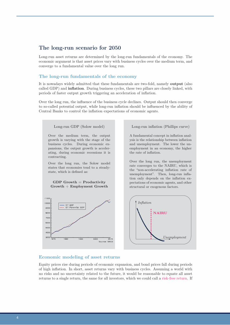
Long-run GDP (Solow model)
Over the medium term, the outputgrowth is varying with the stage of thebusiness cycles. During economic ex-pansions, the output growth is acceler-ating, during economic recessions it iscontracting.
Over the long run, the Solow modelstates that economies tend to a steady-state, which is defined as:
GDP Growth = ProductivityGrowth + Employment Growth
Long-run inflation (Phillips curve)
A fundamental concept in inflation anal-ysis is the relationship between inflationand unemployment. The lower the un-employment in an economy, the higherthe rate of inflation.
Over the long run, the unemploymentrate converges to the NAIRU, which isthe “non-accelerating inflation rate ofunemployment”. Then, long-run infla-tion only depends on the inflation ex-pectations of economic agents, and otherstructural or exogenous factors.
Unemployment
Inflation
NAIRU
Economic modeling of asset returnsEquity prices rise during periods of economic expansion, and bond prices fall during periodsof high inflation. In short, asset returns vary with business cycles. Assuming a world withno risks and no uncertainty related to the future, it would be reasonable to equate all assetreturns to a single return, the same for all investors, which we could call a risk-free return. If

Q u a n t R e s e a R c h b y Ly x o R 5
s t r at e g i c a s s e t a l l o c at i o nissue # 6
however we return to reality and acknowledge the uncertainty of the future world, it wouldalso be reasonable to add an additional term which we call the risk premium, in referenceto the risk aversion of investors. A practical way to understand the mechanism is to breakasset returns down into these two terms:
Asset returns = Risk-Free Rate + Risk Premium
A risk-free return is traditionally described as the guaranteed return obtained over a sethorizon: the short-term rate for a short-term horizon, or the bond yield for a long-termhorizon. During periods of economic expansion, it increases as Central banks hiketheir short rates in order to restrain demand and so limit inflationary pressures. Over thelong run, the risk-free return should equate potential output growth, through the Goldenrule.
The risk premium could be interpreted as the return required by investors in excess ofthe risk-free return, in order to cushion them against uncertainty. During periods ofeconomic expansion, the risk premium decreases, as investors become less risk averseand are willing to accept a lower excess return. Over long-term horizons, risk premiumsshould converge to values that depend solely on the nature of the underlying asset. Standardmodels derived from asset pricing theory then help us identify the specific fundamentaldeterminants tied to a specific asset class.
To determine long-run assumptions, we adopt a “fundamental fair value” approach.
The Two Economic Pillars
Potential Growth
Inflation
⇓
Long-run Returns on Asset Classes
Short Rate =⇒
Government Bonds =⇒
Equities
Corporate Bonds
Commodities
Other Asset Classes
2050: lower bond returns, and a return to standard equity risk pre-miumsAfter the initial step of choosing asset returns models, we use simple statistical tools tocalibrate long-run relationships, and then forecast long-run asset returns in a systematicway. We can then answer the first question: what is the long-run scenario for the next 50years?
Our results highlight a much more favorable outlook for equities than for bonds when com-pared to figures observed over the last 25 years.
6
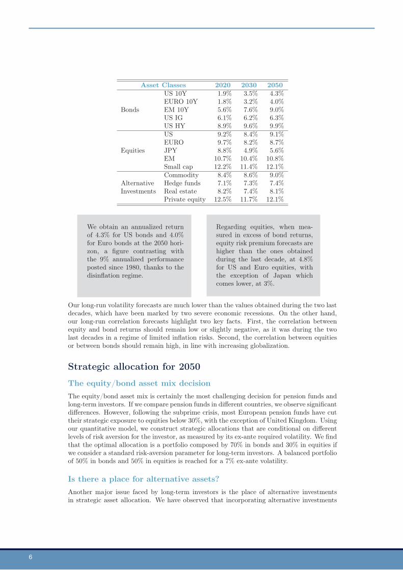
Asset Classes 2020 2030 2050US 10Y 1.9% 3.5% 4.3%EURO 10Y 1.8% 3.2% 4.0%
Bonds EM 10Y 5.6% 7.6% 9.0%US IG 6.1% 6.2% 6.3%US HY 8.9% 9.6% 9.9%US 9.2% 8.4% 9.1%EURO 9.7% 8.2% 8.7%
Equities JPY 8.8% 4.9% 5.6%EM 10.7% 10.4% 10.8%Small cap 12.2% 11.4% 12.1%Commodity 8.4% 8.6% 9.0%
Alternative Hedge funds 7.1% 7.3% 7.4%Investments Real estate 8.2% 7.4% 8.1%
Private equity 12.5% 11.7% 12.1%
We obtain an annualized returnof 4.3% for US bonds and 4.0%for Euro bonds at the 2050 hori-zon, a figure contrasting withthe 9% annualized performanceposted since 1980, thanks to thedisinflation regime.
Regarding equities, when mea-sured in excess of bond returns,equity risk premium forecasts arehigher than the ones obtainedduring the last decade, at 4.8%for US and Euro equities, withthe exception of Japan whichcomes lower, at 3%.
Our long-run volatility forecasts are much lower than the values obtained during the two lastdecades, which have been marked by two severe economic recessions. On the other hand,our long-run correlation forecasts highlight two key facts. First, the correlation betweenequity and bond returns should remain low or slightly negative, as it was during the twolast decades in a regime of limited inflation risks. Second, the correlation between equitiesor between bonds should remain high, in line with increasing globalization.
Strategic allocation for 2050
The equity/bond asset mix decisionThe equity/bond asset mix is certainly the most challenging decision for pension funds andlong-term investors. If we compare pension funds in different countries, we observe significantdifferences. However, following the subprime crisis, most European pension funds have cuttheir strategic exposure to equities below 30%, with the exception of United Kingdom. Usingour quantitative model, we construct strategic allocations that are conditional on differentlevels of risk aversion for the investor, as measured by its ex-ante required volatility. We findthat the optimal allocation is a portfolio composed by 70% in bonds and 30% in equities ifwe consider a standard risk-aversion parameter for long-term investors. A balanced portfolioof 50% in bonds and 50% in equities is reached for a 7% ex-ante volatility.
Is there a place for alternative assets?Another major issue faced by long-term investors is the place of alternative investmentsin strategic asset allocation. We have observed that incorporating alternative investments

Q u a n t R e s e a R c h b y Ly x o R 7
s t r at e g i c a s s e t a l l o c at i o nissue # 6
improves the portfolio return for a given level of risk aversion. We have also noticed thatthe weightings of bonds are fairly similar. Alternative investments are therefore a substitutefor equities.
Interestingly, we find that these optimal weightings of alternative investments are higher thanthe ones implemented in practice. The lack of liquidity of such investments is commonly citedas an explanation. Nevertheless, we can demonstrate that even if we take this drawback intoaccount, the place of alternative investments in strategic asset allocation today is certainlyunder-estimated.
We can now answer the second question about strategic allocation: in whichproportions should equities, bonds, and possibly alternative assets be chosento build a long-term portfolio consistent with this scenario?
• The strategic equity/bond asset mix allocation derived from our long-runassumptions highlights an equity exposure close to 30% for a standardrisk-aversion parameter. This allocation is close to the one exhibited bymost European pension funds, following the subprime crisis.
• There is a place for alternative assets in this strategic allocation. Specif-ically, we find that the weightings of alternative assets could reach 1/3of the overall risky assets, which is higher than the one implemented inpractice. But the lack of liquidity of such investments is a negative factorin implementing tactical asset allocation.
ConclusionThe recent crisis has one great merit. It has reminded us that strategic allocation is akey issue that any institutional investor must address. A long-term strategy needs to beconsistent with a long-run economic scenario. By consistency we mean a strategy thatreflects the world we live in: ageing populations, globalization and ever increasing demandson natural resources. These key themes will have an impact on global output and assetreturns for the years to come. Our quantitative framework accounts for these phenomenonand provides strategic allocations that match a long-run scenario.

8

Q u a n t R e s e a R c h b y Ly x o R 9
s t r at e g i c a s s e t a l l o c at i o nissue # 6
Table of Contents
1 Introduction 11
2 Economic modeling of risk premiums 132.1 The two economic pillars . . . . . . . . . . . . . . . . . . . . . . 152.2 Modeling asset returns . . . . . . . . . . . . . . . . . . . . . . . 172.3 Assessing market risks . . . . . . . . . . . . . . . . . . . . . . . 23
3 Empirical estimation of risk premiums 253.1 Potential output and inflation . . . . . . . . . . . . . . . . . . . 253.2 Asset returns . . . . . . . . . . . . . . . . . . . . . . . . . . . . 263.3 Volatility and correlation . . . . . . . . . . . . . . . . . . . . . . 32
4 Strategic asset allocation in practice 344.1 Building a strategic equity portfolio . . . . . . . . . . . . . . . . 344.2 The equity/bond allocation policy in a strategic asset allocation 364.3 The place of alternative investments in a long-term portfolio . . 38
5 Conclusion 40
A Notations 42
B Macro-economics pillars 43B.1 Modeling economic growth . . . . . . . . . . . . . . . . . . . . . 43B.2 Inflation . . . . . . . . . . . . . . . . . . . . . . . . . . . . . . . 46
C Asset returns models 48C.1 Interest rates . . . . . . . . . . . . . . . . . . . . . . . . . . . . 48C.2 Equities . . . . . . . . . . . . . . . . . . . . . . . . . . . . . . . 49C.3 Currencies . . . . . . . . . . . . . . . . . . . . . . . . . . . . . . 50C.4 Credit . . . . . . . . . . . . . . . . . . . . . . . . . . . . . . . . 51
D Results of regression models 53

10
Q u a n t R e s e a R c h b y Ly x o R 11
s t r at e g i c a s s e t a l l o c at i o nissue # 6
Strategic Asset Allocation∗
Karl EychenneResearch & Development
Lyxor Asset Management, [email protected]
Stéphane MartinettiResearch & Development
Lyxor Asset Management, [email protected]
Thierry RoncalliResearch & Development
Lyxor Asset Management, [email protected]
March 2011
Abstract
To implement strategic asset allocation, we must determine risk and return expec-tations for the various asset classes. Starting from the paradigm that long-run assetreturns are determined by the long-run fundamentals of the economy, a fair valueapproach to building expectations is crucial. This paper proposes to formalize a quan-titative and systematic methodology for optimizing portfolios, from the determinationof long-run fundamental pillars through the modeling of asset returns and the assess-ment of market risks. We apply forecasting models and build in the specific of themain asset classes (equities, bonds and alternative investments) depending on the un-certainties they represent for the risk-averse investor. Our resulting allocations withinthe equity asset class, and with regard to the place of alternative investments, questionthe choices of long-term institutional investors such as pension funds that have shiftedtheir long-run allocations in response to the recent financial crisis.
Keywords: Long-term investment policy, strategic asset allocation, tactical asset alloca-tion, risk premium, long-run economic growth, Solow model, Phillips curve.
JEL classification: E20, E50, G11.
1 Introduction
The recent crisis caused significant damages, with job losses and lower output for the realeconomy, and sell-offs in the equities and credit markets in the financial world. Monetaryand government authorities prevented an outright collapse, by implementing far-reaching,unconventional support policies. Unfortunately, the crisis spread geographically and alsoover time with negative inter-temporal impacts. Pension funds posted major losses whichmay affect pension pay-outs in the future. In particular, their performances was hit as a
∗We are grateful to Jérôme Glachant (University of Évry), Jean-Sébastien Pentecôte (University ofRennes) and Nicolas Rautureau (University of Nantes) for their helpful comments.
12
result of their exposure to underperforming asset classes, such as equities. The roots of thesesignificant losses lie in the investment policies of pension funds.
This issue reveals confusion regarding the nature of investors’ decisions. On the one hand,decisions that are made with respect to structural changes in the economy should relate tothe strategic asset allocation. On the other hand, choices that alter the asset mix in theportfolio to reflect the impact of business cycles over the short to medium term are definedas being part of tactical asset allocation. Logically, changes of strategic allocation should beoccasional, because structural shocks are less frequent than changes in the business cycle.However, a number of events during the past twenty years have defied this logic. Investorsover-weighted equities in the boom years leading up to the dot.com crisis or during the2003-2007 equity bull market, and completely revised their equity/bond asset mix after thetechnological bubble burst, and the subprime financial crisis. Following the financial crisis,most strategic asset allocations have been revised by decreasing equity exposure. Thereis clearly confusion between tactical and strategic allocation, because investors’ long-runassumptions appear to have varied too much during this period.
In recent years, solutions have been developed to limit risks and to guarantee the pensionfunds. Liability-driven investments (LDI) and asset and liability management (ALM) referto those investment policies in which investors focus on monitoring the difference betweentheir assets and their liabilities. By way of illustration, the idea of the LDI solution isto compare the fund’s asset value to the fund’s liabilities and to compare their respectivesensitivities to market factors (Bruder et al., 2010). This leads to the design of portfoliostrategies that will match future pension scheme payments as closely as possible. However,the origin of the problem still remains because the choice of a strategic portfolio is beingderived from long-run assumptions on asset returns.
In academic literature, various approaches have been proposed for forecasting long-runasset returns, including reference to historical values or to economic models. Over the pastdecade, econometric models have been widely used to study the inter-temporal behavior ofasset returns in the presence of macro-economic factors (Campbell and Viciera, 2002). Inthis paper, we propose a comprehensive and systematic approach for determining long-runasset returns. First, we make extensive reference to economic and asset pricing theories forformalizing the long-term behavior of asset returns. In particular, we present the notion offair value of assets, which states that long-run asset returns could be derived from the long-run path of the real economy. Second, we use limited statistical tools to calibrate long-termrelationships between variables, in order to determine long-run asset return forecasts in asystematic manner.
The paper is organized as follows. The second section sets out the theoretical frameworkof our approach for determining long-run asset returns, the role of output and inflation aseconomic fundamentals, and the derivations of risk premiums for key asset classes. In thethird section, we present the empirical results obtained using macro-econometric regressionmodels. These results are presented with respect to regional variations, and feature forecastson asset returns from horizons varying from 2020 to 2050. Section four derives long-termportfolios from our risk and return expectations. In particular, we describe a number ofpossible strategic allocations by considering a pure equity portfolio, then adding bonds, andfinally alternative investments. Section five concludes by opening the door to a comprehen-sive analysis framework that encompasses both strategic and tactical asset allocations.
Q u a n t R e s e a R c h b y Ly x o R 13
s t r at e g i c a s s e t a l l o c at i o nissue # 6
2 Economic modeling of risk premiumsThe decision-making process for a strategic allocation requires long-term expectations ofasset class returns, volatilities, and correlations as inputs. One popular method consists inusing historical figures as a guide for the future. This method is said to be unconditional,meaning that the expected returns are based solely on historical returns, and so do not takeinto account any global shocks or structural economic changes that could arise. Here aresome examples:
• The Bond returns observed during the 80s and 90s may not be repeated in the future,because disinflation is unlikely to re-occur to the same extent;
• The stock/bond correlation depends on the inflation environment;
• The commodity returns depend on population growth and demand from emergingcountries.
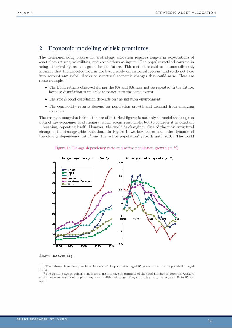
The strong assumption behind the use of historical figures is not only to model the long-runpath of the economies as stationary, which seems reasonable, but to consider it as constant– meaning, repeating itself. However, the world is changing. One of the most structuralchange is the demographic evolution. In Figure 1, we have represented the dynamic ofthe old-age dependency ratio1 and the active population2 growth until 2050. The world
Figure 1: Old-age dependency ratio and active population growth (in %)
Source: data.un.org.
1The old-age dependency ratio is the ratio of the population aged 65 years or over to the population aged15-64.
2The working-age population measure is used to give an estimate of the total number of potential workerswithin an economy. Each region may have a different range of ages, but typically the ages of 20 to 65 areused.
14
population is expected to decelerate across the regions, with particularly a growing share ofold-age people. We note that these trends should be more pronounced in Europe and Japan.These demographic changes should be associated with changes of saving rates, public sectorexpenditures and economic growth.
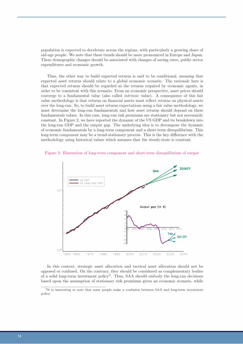
Thus, the other way to build expected returns is said to be conditional, meaning thatexpected asset returns should relate to a global economic scenario. The rationale here isthat expected returns should be regarded as the returns required by economic agents, inorder to be consistent with this scenario. From an economic perspective, asset prices shouldconverge to a fundamental value (also called intrinsic value). A consequence of this fairvalue methodology is that returns on financial assets must reflect returns on physical assetsover the long-run. So, to build asset returns expectations using a fair value methodology, wemust determine the long-run fundamentals and how asset returns should depend on thesefundamentals values. In this case, long-run risk premiums are stationary but not necessarilyconstant. In Figure 2, we have reported the dynamic of the US GDP and its breakdown intothe long-run GDP and the output gap. The underlying idea is to decompose the dynamicof economic fundamentals by a long-term component and a short-term disequilibrium. Thislong-term component may be a trend-stationary process. This is the key difference with themethodology using historical values which assumes that the steady-state is constant.
Figure 2: Illustration of long-term component and short-term disequilibrium of output
In this context, strategic asset allocation and tactical asset allocation should not beopposed or confused. On the contrary, they should be considered as complementary bodiesof a solid long-term investment policy3. Thus, SAA should embody the long-run decisionsbased upon the assumption of stationary risk premiums given an economic scenario, while
3It is interesting to note that some people make a confusion between SAA and long-term investmentpolicy.

Q u a n t R e s e a R c h b y Ly x o R 15
s t r at e g i c a s s e t a l l o c at i o nissue # 6
TAA should allow for adjusting to the business cycle within which risk premiums are time-varying. Lastly, very short-term investment decisions (like for example achieving a volatilitytarget) should be considered as market timing (MT) and are not relied to risk premium (butto the market sentiment).
MT
TAA
SAA
1 Day – 1 Month 3 Months – 3 Years 10 Years – 50 Years
In conclusion, our approach of SAA could be illustrated by the following scheme. First,we identify two representative economic fundamentals (output and inflation) and we build along-run economic scenario for these two variables. Second, we derive long-run asset returnsfrom this economic scenario. The long-run short rate is directly obtained by adding togetheroutput and inflation. To obtain the long-run government bond return, we add a bond riskpremium to the long-run short rate. Finally, the expected returns of the other asset classesare derived from the specific risk premium associated with the nature of the asset class.
The Two Economic Pillars
Potential Growth
Inflation
⇓
Long-run Returns on Asset Classes
Short Rate =⇒
Government Bonds =⇒
Equities
Corporate Bonds
Commodities
Other Asset Classes
2.1 The two economic pillars
The long-term outlook for the economy has been and will continue to be debated extensively.Central banks and governments pay close attention to the economy’s long-term prospects inorder to optimize their monetary and budgetary policies4.
2.1.1 Potential output
Economic output, also known as gross domestic product (or GDP), represents the country’snominal aggregated value of all final goods and services. Typically, output grows stronglyduring periods of economic expansion, and shrinks during a recession. But this cyclical effectvanishes when one look at longer horizons of 20, 30 or 50 years, and we are left with thecomplex task of describing the long-term outlook for the economy. Does output still behavelike a longer cycle, reverting to a somewhat long-term average level? Or does it follow a
4For illustration, the US Central bank operates under a dual mandate to achieve both price stability andsustainable growth.
16
steady path in a given direction with quantifiable intensity? To achieve this, economists gen-erally define so-called potential output as a measure of the economy’s productive capacity5.In practice, the full employment output and the maximum sustainable output consistentwith a stable rate of inflation are suitable measures for estimating this capacity. A broadtheoretical consensus has been obtained, stating that modeling potential output relies onfocusing on the drivers of growth on the supply side of the economy.
Inspired by the neo-classical theory of production, the Solow model presented in Ap-pendix B.1.1 has achieved broad recognition for its ability to formalize the conception of along-term trend followed by the economy. It assumes that output growth is driven by growthin labor input (or demography) and the accumulation of physical capital. The model alsoimplicitly assumes the existence of factor productivity, a residual part of the output growththat cannot be attributed to the two previous production factors6. Basically, Solow (1956)predicts that output growth should converge towards equilibrium7. It states that the econ-omy tends to a steady-state, where output growth is only due to long-run constant andexogenous production factors, namely growth in the labor force and growth in productiv-ity8:
• Growth in the labor forceThe rationale behind the concept of stable long-run employment growth makes refer-ence to a “natural” unemployment rate. Over the medium term, the unemploymentrate could be above or below its natural level. Typically, periods of faster economicgrowth trigger stronger employment growth, and so lower the unemployment rate.This situation occurs when output exceeds its potential level (positive output gap).Indeed, a positive output gap triggers tensions on resources of production, and the sup-ply of workers becomes scarcer, as explained by Okun’s law, as presented in AppendixB.2.3. However, the output gap becomes null over the long term, so the unemploymentrate converges to its natural level.
• Productivity growthProductivity is a measure of output per unit of input (worker, machine, etc.). Econo-mists have attributed productivity growth to many causes besides technological pro-gress, for example changes in the rate at which capital is used, changes in the quality oflabor or the amount of human capital, changes in businesses’ organization or culture,or productivity shocks. Meanwhile, as a residual in Solow model, it remains technicallydifficult to model or predict. Nevertheless, over the long term, it is possible to use avariant of Okun’s law to define a long-run productivity growth rate, meaning cyclicallyadjusted.
5An other common approach consists in estimating a long-run stochastic trend to quantify the steadypath of long-run output (Beveridge and Nelson, 1981).
6The role of productivity has been validated empirically by former academic works that found that asignificant part of output changes are explained by the Solow residual (Kydland and Prescott 1991, King andRebelo 1999, Tang 2002). Today, this assumption is not completely accepted (Francis and Ramey, 2005).
7There also exist statistical approaches that aim at estimating the potential output. For instance,Hodrick-Prescott and Kalman filters are often used to extract directly the trend from the output. Thesemethods do require analysts to make assumptions about how the filters are structured, including the valuesof one or more parameters. However, they could not be used to perform forecast of the output.
8Solow specifically models a closed economy where output growth is attributed to the dynamics of capitalaccumulation and to some effective labor force growth that is assumed to be constant and exogenous. Themain result is that, given an initial amount of capital and fixed exogenous savings rate, a steady-state isreached when investment equals depreciation of capital. Capital growth and therefore potential outputgrowth are then constant and equal to the sum of employment growth and productivity growth, after thestock of capital reached its steady-state level.
Q u a n t R e s e a R c h b y Ly x o R 17
s t r at e g i c a s s e t a l l o c at i o nissue # 6
Remark 1 The macro-economic framework based on the Solow model is particularly rel-evant for strategic asset allocation. The other growth economic models (Ramsey model,endogenous growth models or DSGE) are less suitable because they address both tactical andstrategic asset allocations.
2.1.2 Long-run inflation
Inflation is traditionally defined as the rise in the general level of prices of goods and servicesin an economy. Over the medium term, variations of inflation are usually attributed tobusiness cycles. Typically, inflation accelerates (resp. decelerates) when output exceeds(resp. falls below) its natural level. Indeed, excessive output requires intensive use of inputswhich eventually puts pressure on prices. We generally refer to the well-known Phillipscurve to illustrate these stylized facts (Phillips 1958, Cahuc and Zylberberg 2004). In thistheory, high inflation is associated with low unemployment (Appendix B.2.1). When theunemployment rate falls (resp. rises) below (resp. above) a specific level, then inflationaccelerates (resp. decelerates). The specific unemployment level that remains neutral withrespect to inflation is called the “non-accelerating inflation rate of unemployment” or NAIRU(Appendix B.2.2).
Over the long term, when the economy converges to equilibrium, output and the unem-ployment rate should converge respectively to potential output and to a natural unemploy-ment rate, commonly referred as the NAIRU (Blanchard and Katz, 1997). In other words,output and unemployment reach levels that are defined as sustainable and consistent withstable inflation (Bruno and Easterly, 1998). Is there any truth behind this hypothesis? Letus consider rational economic agents. In order to stabilize their purchasing power, they de-mand higher wages when they expect inflation to rise. This is called the long-run neutralityof inflation: variations of inflation are fully passed on to the nominal value of economicvariables, keeping their real value constant. Therefore, rational expectations imply thatlong-run variations in inflation should have no impact on the equilibrium level of actualoutput.
However, we have still not addressed the crucial question of the choice of a long-runinflation rate. There is broad agreement among economists that long-run inflation is onlya monetary phenomenon, and could be related to monetary policy (quantitative theory ofmoney). Simply stated, the quantity of money in the economy should be conditional on thelevel of inflation that the Central banks assume to be consistent with sustainable output.A consequence is that Central banks must establish their credibility in fighting inflation. Ifnot, agents would bet on the fact that Central banks will expand (resp. decrease) the moneysupply rapidly enough to prevent recessions, even at the expense of exacerbating inflation.In fact, the main Central banks declare an official (medium-term) objective for inflation,also called an inflation target. These targets are therefore reliable candidates for long-runinflation (Bernanke et al. 1999, Friedman 2003, Woodford 2003).
2.2 Modeling asset returns
According to the economic theory, the return on capital is closely tied with potential growth,and capital stock in particular. From a micro-economic point of view, the level of returnon capital should result from the opposing forces of supply and demand for capital. Awell-known optimal condition derived from neo-classical theory is achieved when the realreturn on capital is equal to the marginal productivity of physical capital (Appendix B.1.3).In other words, supply and demand reach equilibrium when adding one dollar of physical

18
capital is equivalent to buying one dollar of the firm’s asset. From a macro-economic pointof view and according to the Solow model, this equality could be derived in a normativerule, also called the Golden rule which states that the real return on capital consistent withthe maximization of output per worker is equal to real potential output growth (Phelps,1961). What then is the relationship between this synthetic real return of capital derivedfrom the economic theory, and the returns obtained from equities, bonds, and other assetclasses? As suggested by Baker et al. (2005), the mapping between the real return of capitaland asset class returns is completely straightforward only under the assumption of constantrisk premiums. According to the asset pricing theory, risk premiums should reflect investors’assessments of the fundamental risks given by the economy and investors’ sensitivity to theseinherent risks, namely their risk aversion. From an investor’s point of view, risk premiumsare interpreted as excess returns required in order to buy riskier assets rather than risk-freeassets. Lucas (1978) shows that, over the medium term, risk premiums and asset returnsvary with the business cycle. More precisely, they are linked through consumption-basedmodels (Campbell, 1999) and production-based models (Cochrane, 1991). Over the longterm, risk premiums should stabilize as the influence of the business cycle disappears. Thechallenge then consists in estimating the long-run values of asset returns.
2.2.1 Short-term interest rates
Short-term interest rates are the principal instrument used by Central banks to implementtheir monetary policies. They use the short rate in order to attain a set of objectivesoriented towards price stability and sustainability of growth. Let us consider a situationwhere inflation increases to a level that is not consistent with a sustainable output growth.Typically, Central banks could react by hiking interest rates in the hope of stifling demand(consumption and investment), and thereby reducing output to a more sustainable level.The Taylor rule formalizes this idea by quantifying the intensity of change in the short ratethat Central banks should apply in response to observed divergences of actual from targetinflation rates and of output from potential output9. One key result of this rule stipulatesthat when inflation exceeds its target, not only should the short rate be increased, but itshould also overreact to inflation so that the real short rate increases.
Over the long term, the Taylor rule simply states that the short rate converges to thesum of long-run inflation and a long-run real short rate, because divergences in outputand inflation from their equilibrium levels vanish over this horizon (Appendix C.1). Onthe one hand, the Fisher parity tells us that these two variables are not related, meaningthat any change in long-run inflation should have no impact on the long-run real shortrate. This is the case if, and only if, the long-run nominal interest rate adjusts in stepwith the rise of inflation. On the other hand, as previously mentioned, the long-run realshort rate is generally viewed as an equilibrium level alongside the steady-state path of theeconomy. According to the Golden rule, it can be set equal to real potential output growth.It is therefore assumed that, at equilibrium, the long-run short rate is the sum of long-runinflation and real potential output growth.
2.2.2 Bond returns
Sovereign bonds The key notion is that bond prices react conversely to shifts in interestrates, and that these shifts typically occur in tandem with business cycles. For example,bonds prices rise as a consequence of falling bond yields, when the economy is slowing
9The Taylor rule does not verify the Tinbergen Rule, which states that with only one policy instrument,policy can only achieve one goal.
Q u a n t R e s e a R c h b y Ly x o R 19
s t r at e g i c a s s e t a l l o c at i o nissue # 6
and/or inflation is decelerating. Typically, during difficult economic times Central bankslower their short-term rates in order to restore the conditions required for an economicexpansion, and this cut partially spreads to long-term rates. Financial theory formalizesthe relation between short-term rates and long-term rates through the rational expectationsmodel of the term structure: if long-term rates are higher than short-term rates, it meansthat investors anticipate higher short rates (Lutz, 1940). A key result is that for an investor,holding a long-term bond would be the same as rolling a short-term rate over the sameperiod (Appendix C.1). However, there is empirical evidence10 that the difference betweenlong-term rates and short-term rates (the term spread) is not only related to future short-term rates expectations, but may also be influenced by other factors. Following the economictheory, long-term rates should be especially sensitive to the government policy, while short-term rates are more sensitive to monetary policy11. From the investor’s point of view, theslope of the yield curve is effectively a bond risk premium required in order to compensatefor higher uncertainty over a longer period. Moreover, following Lucas (1978), this termstructure spread could logically vary alongside business cycles. The intuition is that investorsprefer a smooth consumption stream rather than very high consumption at one stage of thebusiness cycle and very low consumption at another stage. A logical hedging method is tosubstitute bonds of different maturities. A key result of this is that the slope of the yieldcurve should rise (resp. fall) during economic slowdowns (resp. expansions), meaning thatthe bond risk premium required by the investor to buy a long-term bond rather than ashort-term bond should rise (resp. fall).
Over the long term, the bond risk premium is supposed to stabilize because the influenceof business cycles should vanish. However, this bond risk premium should remain positiveas the investor still requires an excess return over the short-term rate to compensate forhigher uncertainty over longer time horizons. How then does this uncertainty embody long-run economic risks that characterize the long-run path of the economy? According to theeconomic theory, these risks could be related to both monetary and government policies.For Central banks, a failure to control inflation would lead to the erosion of the real bondreturn at maturity. In practice, long-run inflation volatility is a measure of this uncertainty.For governments, a failure to control their budget deficits could trigger higher bond yields,undermining the value of previous bond issues. Here again, the uncertainty surroundingthis issue is clearly indicated by the long-run budget balance (or debt) over GDP ratio. Thelong-run bond risk premium can thus be seen as an indicator of the long-term credibility ofmonetary and government policies. It follows that a long-run bond yield should thereforebe linked to a long-run short rate and a bond risk premium that is positively related tolong-run inflation volatility and the equilibrium deficit/GDP ratio. Finally, it is possibleto mechanically derive a long-run bond return from the long-run path of the 10-year bondyield.
Corporate bond returns Corporate bonds provide the same payoff structure as sovereignbonds, but are more risky because a company’s capacity to service its debt is uncertainwhereas sovereign bonds have the status of safe assets12. It is therefore only to be expected
10Note that the hypothesis that long-term yields equal an average of future expected short-term yields isa statement about the unpredictability of bonds’ excess returns. However, Fama and Bliss (1987) find thatthe spread between the m-year forward rate and the 1-year yield predicts the 1-year excess return of them-year bond, with a R2 of about 18%. Campbell and Shiller (1991) find similar results while forecastingyield changes using yield spreads. Cochrane and Piazzesi (2005) extend these results for long-term bonds.
11For example, in the IS-LM model of Clarida and Friedman (1983), long-term rates affect the IS curvewhereas short-term rates influence the LM curve.
12This status of safe assets is especially pronounced during periods of high uncertainty on the economy,with investors fleeing from risky assets to take refuge in government bonds. However, since 2010 this status
20
that corporate bond should offer a higher expected return compared to sovereign bonds, tocompensate for their higher risk. In yield terms, this means that the difference (also calledthe credit spread) between the corporate bond yield and the sovereign bond yield should bepositive. The fundamentals of this theory were formally propounded by Merton (1974), whodemonstrated that the credit spread is closely linked to a company’s leverage and its assetsvolatility, as these two variables provide information on the probability of default (Jones etal., 1984). During economic recessions, this uncertainty regarding a company’s capacity toservice its debt is exacerbated due to the increasing probability of default.
Over the long term, credit risk premiums are not supposed to vary because businesscycles are eliminated. In particular, the default rate should converge towards a long-runlevel, which should be related to long-run output growth, and the volatility on equities shouldalso stabilize close to a long-run average. Long-run corporate bond yields can therefore bebroken down into the long-run sovereign bond yield plus a credit risk premium derived fromthe long-run default rate and volatility. As for sovereign bonds, the long-run corporate bondreturn can be derived from the long-run path of corporate bond yields.
Remark 2 Emerging bonds combine the characteristics of both sovereign and corporatebonds. The difference between emerging bond yields and US government bond yields (alsocalled the emerging bond spread) is commonly regarded as a measure of an emerging econ-omy’s creditworthiness. Typically, a widening of the emerging bond spread is associated withgreater uncertainty regarding a country’s economic and/or political situation. Investors fo-cus in particular on the balance of payments structure13 when assessing a country’s financialhealth. In fact, uncertainty about the capacity of emerging economies to finance their eco-nomic growth is higher when trade balance and/or budget deficits are large. Also, emergingspreads may depend on currency risk as well as liquidity conditions. An emerging economycrisis is generally characterized by large foreign capital outflows and the depreciation of thelocal currency. Using the same methodology as for corporate bonds, we then find that long-run emerging bond yields can be broken down into US government long-run bond yields plusan emerging bond risk premium derived from the long-run current account position and thevolatility of emerging equities. Lastly, long-run emerging bond returns can be derived fromthe long-run path of emerging bond yields.
2.2.3 Equity returns
Equities differ substantially from bonds in that they do not have a defined maturity andtheir future cash flows are unknown. However, as with bonds, the assumption of no arbi-trage requires that equities should be priced at their discounted intrinsic values, meaningthe present value of their expected cash flows. The discount rate is either interpreted asthe cost of capital from the firm’s point of view, or as the expected equity return from theinvestor’s point of view. Considering the firm’s point of view, equity prices are then inverselyrelated to the cost of capital (also positively correlated to the expected cash flows). In par-ticular, a lower (resp. higher) cost of capital should be associated with higher (resp. lower)equity prices (Campbell and Shiller, 1988). But does this means that equities outperform(resp. underperform) sovereign bonds? No, because this cost of capital makes no distinctionbetween the cost related to the level of the risk-free interest rate and the one related to thehas been undermined due to increasing doubts about European countries’ capacity to service their debt.
13In economics, the current account is one of the two primary components of the balance of payments,the other being the capital account. The current account is the sum of the balance of trades (exports minusimports of goods and services), net factor income (such as interest and dividends) and net transfer payments(such as foreign aid). A current account surplus increases a country’s net foreign assets by the correspondingamount, and a current account deficit does the reverse.
Q u a n t R e s e a R c h b y Ly x o R 21
s t r at e g i c a s s e t a l l o c at i o nissue # 6
underlying characteristics of the firm. Considering the investor’s point of view thus helps usto assess the behavior of this equity risk premium. Cochrane (2001) revisits Lucas’ modelin order to demonstrate a formal link between equity risk premiums and business cycles14.Simply stated, he explains that economic recessions trigger higher equity risk premiums,because the investor becomes particularly averse to buying assets that fail to hedge himagainst unwelcome changes in his consumption.
However, knowing that over the long-run, business cycles vanish and no longer influenceexpected returns, where do we stand regarding the behavior of equity risk premium over longhorizons? Equity prices should reflect only the long-run expectations of the rational investor.Any deviation of the market price of equities from their fair value should be interpreted as anevidence of market inefficiency and should disappear. For a long-term analysis, a very wellsuited approach is proposed by Gordon (1959), which assumes that future dividends shouldgrow at a constant rate and that the expected return on equity (cost of capital) requiredremains constant as well (Appendix C.2). In particular, the model proposes a breakdown ofthe equity expected return in the sum of a risk-free return and a pure equity risk premium.It is then possible to resolve the model for the equity risk premium which equals the sum ofthree elements.
• The first is dividend yield (calculated as the dividend over price ratio). This variableis commonly assumed to be constant. Campbell and Shiller (1998) state that over longtime horizons, the dividend yield forms a stationary time-series. Specifically, dividendyields are highly persistent, and any deviation from a long-term average should beregarded as temporary. However, the last decade has produced growing evidenceof slow time-varying dividend yields related to demographic variables (Favero et al.,2009). In brief, these studies show that dividend yield is inversely related to the ratioof middle-aged to young population. A long-run dividend yield should therefore beconsistent with demographic assumptions.
• The second is constant dividend growth rate, which is assumed to be consistent withearnings growth. Dividends represent a share of the company’s earnings which isempirically stable over the long run, despite a long period of structural decline duringthe 90s15. Also, earnings growth is supposed to be consistent with long-run outputgrowth. Indeed, the output produced is the overall income which is distributed betweenwages and earnings. Earnings may therefore grow faster than overall income for a time,but not indefinitely.
• The third is more commonly embodied by long-run government bond yields ratherthan long-run short rates. The equity risk premium is therefore defined by referenceto the yield on a government bond.
Remark 3 An interesting case is that of small caps, which are defined as equities with lowmarket capitalizations. Traditionally, their equity risk premiums are higher than for largecaps, because they present a liquidity risk and greater uncertainty regarding their future cashflows. Small caps usually underperform large caps during a recession. The natural wayof assessing long-run returns on small caps is to sum the long-run equity return and thehistorical excess return of small caps over large caps.
14Bansal and Yaron (2004) find encouraging empirical results, especially by using specific forms of utilityfunctions.
15During this period, we observe a structural decline of the payout ratio (the share of a company’s earningsout in dividends) due to changes in corporate management policies. The low cost of capital promptedcompanies to finance their corporate investments through debt rather than equity.
22
2.2.4 Returns on other asset classes
Commodities Unlike equities and bonds, the existence of a commodity risk premium –excess return of commodities over the risk-free rate – has been the object of much debate16.The risk premium theory advanced by Keynes (1923) relates futures prices to anticipatedfuture spot prices, arguing that speculators bear risks and must be compensated for theirrisk-bearing services in the form of a discount, known as normal backwardation17. On theother hand, the theory of storage as proposed by Kaldor (1939), postulates that the returnfrom purchasing a commodity at time t and selling it forward for delivery at time T , shouldbe equal to a cost of storage minus a convenience yield. The empirical evidences for theexistence of time-varying commodity risk premiums related to business cycles are strong(Deaton and Laroque, 1992). Typically, periods of strong global demand are associatedwith low inventories, implying a surge of commodities prices. However, the evidence fora long-run commodity risk premium is patchy. One could therefore argue that over longtime horizons, commodity returns should be close to a risk-free rate18. However, froman economic point of view, the necessity of leaving a share of natural resources for futuregenerations to use, and the growing role of emerging economies could structurally driveprices higher, justifying a risk premium over the long term. Long-run commodity returnscould thus be defined as the sum of the long-run short-term rate and a risk premium. Thislatter should relate to the long-run balance between resources and consumption, potentiallyproxied by the combination of global output growth and the emerging economies’ share ofglobal output (USDA, 2010).
Other alternative asset classes Since the early 90s, institutional investors’ interest in“alternative” asset classes has grown significantly. Higher volatility in the equity marketsand record low bond yields have led investors to demand alternative sources of return. Themajor categories include real estate, private equity and hedge funds. Over the long term,the empirical evidence for return on alternative assets confirms certain key characteristics(Roxburgh et al. 2009, Fugazza et al. 2007, Phalippou 2007). First of all, there is thepotential for additional diversification. Alternative assets generate different returns charac-teristics than traditional asset classes. Their returns are to a certain degree less correlatedwith traditional equity and fixed income, thereby mitigating portfolio risk. Also, alternativeinvestments are often required to provide superior risk-adjusted performances compared totraditional investment, mainly to offset their higher degree of illiquidity and prevailing sus-picions regarding their transparency. Because of this relative illiquidity, they are thereforebest suited for long-term horizons. Think of institutional investors that are willing to takea longer-term view when investing in these alternatives, which sometimes impose lock-ups.However, unlike equities and bonds, in the absence of a clearly identifiable body of theo-retical work, it is not possible to propose a consistent fair value framework. We therefore
16The return from holding physical commodities derives from both their price appreciation and the eco-nomic benefit of physical commodity storage. In contrast, the return on a commodity futures contract takesinto account the price appreciation of the physical commodity, a collateral yield that is the interest earnedon the US Treasury bills used as collateral for the futures position, and a yield realized based on the futuresterm structure. This last source of return on commodities futures is called the roll yield and represents thedifference between the change in futures prices and the change in the spot price, at any time. These changesare due to the convergence of futures contracts with the spot price as the contracts approach expiry.
17The market is said to be in backwardation when futures prices are lower than spot prices. This situationallows investors to earn money from buying the discounted futures contracts, which continuously roll up tothe higher spot price. In this case investors capture a positive roll yield. When the opposite occurs, themarket is said to be in contango.
18It is worth mentioning that commodities are traditionally considered to be a good hedge against inflationbecause they represent a cost for consumers and producers and are therefore an underlying source of inflation.
Q u a n t R e s e a R c h b y Ly x o R 23
s t r at e g i c a s s e t a l l o c at i o nissue # 6
propose to define the long-run returns on alternative asset classes in terms of their historicalrelative performances with traditional asset classes.
Currencies When assessing the sources of return on foreign currencies, financial theoryemphasizes equilibrium relationships between interest rates differentials across various eco-nomic regions, as well as differences in purchasing power between countries. In particular,uncovered interest rate parity postulates that, for domestic investors, an attractive interestrate differential in favor of a foreign country, should be reflected in the corresponding ex-change rate so that investors willing to trade this spread see their profits offset once theyconvert the invested currency back to the currency of the domestic country (Frenkel andLevich, 1975). However, some empirical evidence effectively contradicts this no-arbitragecondition, which is exploited using the so-called carry trade. From an investor’s point ofview, these facts suggest the existence of a time-varying currency risk premium. Alterna-tively, economic theory introduces the notion of a real exchange rate, defined as the nominalexchange rate adjusted by the differential between the price of goods of two countries. Overthe medium term, real exchange rates vary alongside changes of business conditions. Coun-tries with low real short rates, large trade deficits, and negative output gaps tend to beassociated with lower real exchange rates. But over the long term, the real exchange rateshould stabilize. This theory is expressed through purchasing power parity, which statesthat a basket of goods should have the same price worldwide after nominal exchange ratesare taken into account. This implies that long-run exchange rates should be determined bylong-run inflation differentials between economies. Relative stabilization of long-run infla-tion differentials should generally be consistent with negligible currency returns. It is worthnoting that structurally, these mechanisms should favor emerging currencies over developedones. Indeed, as long as an economy is categorized as emerging, it should exhibit higherinflation as a result of the Balassa-Samuelson effect19, which leads to the appreciation ofits real exchange rate. On the other hand, convergence of long-run inflation differentialsbetween developed countries should be consistent with limited currency returns.
2.3 Assessing market risks
2.3.1 Volatility
In its generic formulation, volatility is traditionally related to the quantity of risk embodiedin the real and financial worlds. Low volatility is usually interpreted as limited uncertaintyregarding the future growth of the economy and/or assets, and therefore as low risk. TheUS stock market exhibits historical volatility of around 15% when calculated over the twolast decades, 14% if we consider long-term data. Bonds exhibit significantly lower risk whenmeasured by their volatility, at 9%. Traditionally, volatility is considered to be station-ary with mean-reverting properties, and can therfore be forecast using econometric tools.Typically, these methods postulate that periods of high (resp. low) volatility are followedby periods of low (resp. high) volatility. However, from an economic point of view, theseperiods of high (resp. low) volatility could be related to fundamental volatility, meaningthe volatility of output or/and inflation (Tang 2002, Diebold and Yilmaz 2010). By wayof illustration, the “Great Moderation” in the volatility of economic activity is often datedto the mid-eighties, and has contributed to a structural decline in equity, credit and bondvolatility. The case of commodities is especially interesting, with the oil price shocks of
19The least developed countries have a manufacturing sector in which productivity gains increase rapidly.The resulting salary increases spread to all other sectors of the economy – notably services where theproductivity gains are weaker – and result in structurally stronger inflation. At a more or less rapid pace,price levels in developing countries converge with those of advanced countries.
24
the seventies showing a positive relationship between financial and fundamental volatilities.Regarding other alternative assets, their volatility is allegedly related less to fundamentalsand more to liquidity risk. However, there are differences between alternative assets. Forexample, hedge funds volatility is historically half that of equities, whereas private equityvolatility is twice as high.
Over the long term, the reference to historical figures is more commonly admitted thanfor returns, due to the statistical properties of volatility. However, a long-run volatilityforecast will have to be consistent with the one of the economic pillars. More specifically, ifone expects deviations between output and its potential levels to be limited in the future,and/or inflation to be kept under control by Central banks, then fundamental volatilitywill be lower, resulting in a low level of volatility in the markets. Bond volatility will beclosely linked to inflation volatility, whereas the volatility of equities and credit markets willbe linked to both output and bond yield volatility. Also, expected stock and bond marketvolatility will depend upon the degree of diversification. For example, it would seem logicalto forecast a decline in emerging market volatility. Volatility on small caps should remainhigher than the one on large caps, as these stocks exhibit a specific liquidity risk and higheruncertainty. Regarding commodities, dwindling resources and the growing role of emergingcountries suggests that volatility should not diminish. For alternative assets, it would makesense to forecast future volatility consistently with past volatility, especially for hedge fundswhereas real estate and private equity may be influenced more by equity volatility.
2.3.2 Correlation
The correlation between stock and bond returns is generally positive over time, meaning thatrising (resp. falling) equity returns are associated with rising (resp. falling) bond returns.An interpretation of this positive correlation is derived from the present value model, whichprices equities using the discounted value of future dividends: falling bond yields (positivebond returns) lift the fair value of equities (positive equity returns). However, this correlationcan be influenced by stock market uncertainty and economic considerations. First, periods of“flight to quality” show a negative stock/bond correlation, with large outflows from equitymarkets that find refuge in “safe” government bonds (Ilmanen, 2003). Second, periodsof low inflation are also associated with negative stock/bond correlation, when investorsbecome much less sensitive to changes in bond yield levels. Credit markets tend to bepositively correlated with equity markets as their risk premiums exhibit the same kind ofcorrelation with business conditions, while their correlation with sovereign bonds is unclear.The correlation of commodities with other asset classes is ambiguous, especially due totheir close relationship with inflation. The case of other alternative asset classes intuitivelysuggests that they should exhibit a low level of correlation with traditional asset classes, asthey are supposed to offer a high degree of diversification.
As for volatility, over the long term, the reference to historical figures is more commonlyadmitted than for returns. However, this long-run forecast of correlation must be consistentwith the long-run outlook on economic pillars, especially inflation (Li, 2002). The correlationbetween traditional asset classes and alternative asset classes should remain constant, andshould therefore be derived from historical value. The correlation between distinct marketswithin a specific asset class should depend on the degree of globalization that is expected overthe long term. The intuition is that globalization should reinforce the correlation betweenequity markets, and also between bond markets20.
20The decline of home bias is well documented by economic studies (see e.g. Sørensen et al., 2007).
Q u a n t R e s e a R c h b y Ly x o R 25
s t r at e g i c a s s e t a l l o c at i o nissue # 6
3 Empirical estimation of risk premiums
The objective of this empirical section is to set out forecasts for different long-term horizons(2020, 2030 and 2050). First we provide forecasts for economic pillars, and then we describeour methodology for determining long-term views on returns from different asset classes.These will be used as inputs for a strategic asset allocation. We distinguish between thefollowing regions: US, Euro, Japan, Pacific ex Japan (Australia) and Emerging countries.We use a large body of annual data from January 1970 to September 2010 provided by theIMF, OECD, the World Bank and Datastream21.
3.1 Potential output and inflation
We use forecasts provided by various organisms as inputs, provided they adopt the sameapproach as we do. More specifically, they must make reference to the theory derived fromthe Solow growth model. They should also use economic tools such as the Phillips curveand the NAIRU for determining long-run inflation. Finally, they should consider the long-run structural changes expected for the coming years, such as demographic changes22 andglobalization. Using forecasts of different organisms, we observe some differences whichmay be explained by different approaches regarding the long-run determinants of economicfundamentals. We build a synthetic forecast by averaging the cited organisms’ forecasts,taking into account differences in terms of horizons.
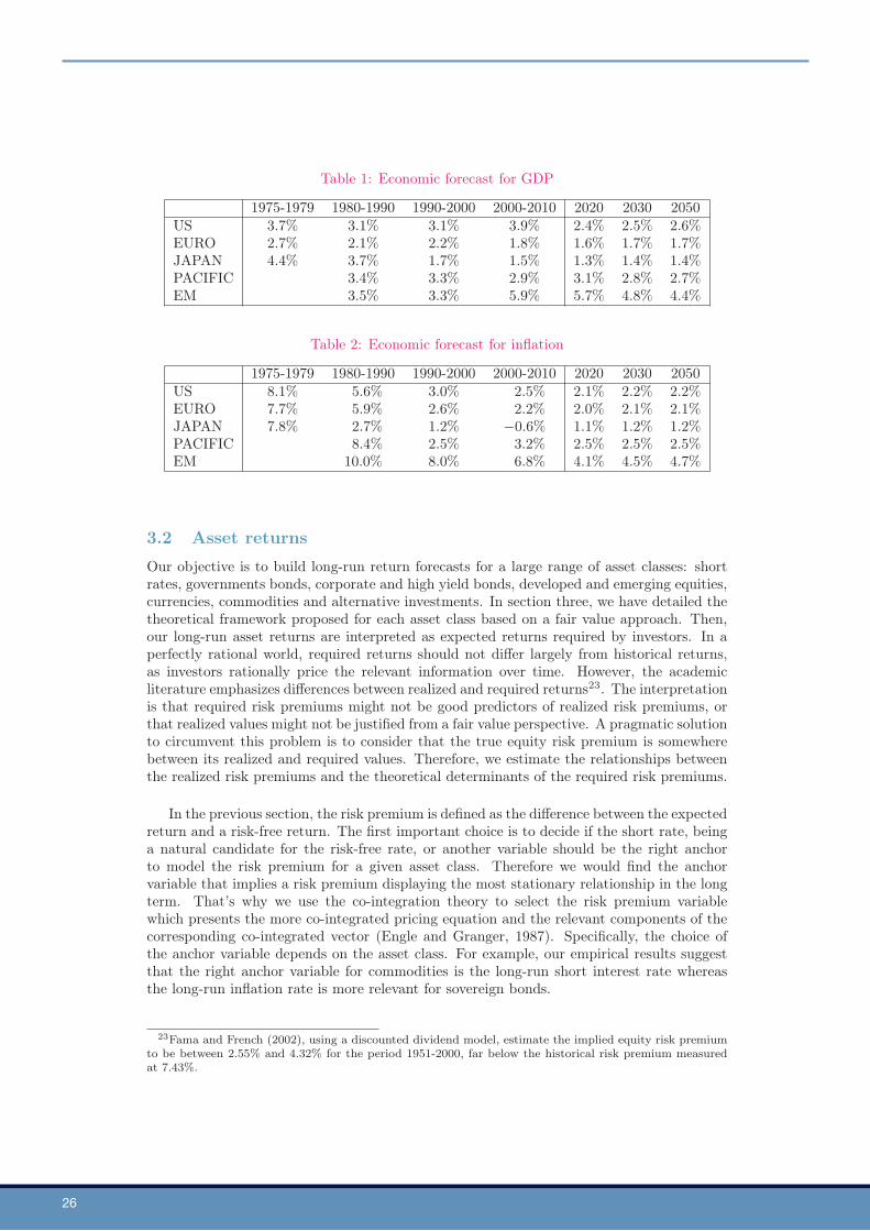
For the 2050 horizon, potential GDP growth is close to 2% for developed countries, buthigher for the US (2.6%) than for the eurozone (1.7%) and Japan (1.4%). These forecastsare lower than values obtained during the past three decades, mainly due to a lower workingpopulation growth forecast. Emerging potential GDP growth converges with that of devel-oped countries, but still remains higher at 4.4%. Inflation stabilizes between 2.1% and 2.2%in the US and the eurozone, at 1.2% in Japan, and at 4.7% in emerging countries. Theselevels are lower than those obtained during the past three decades which were characterizedby structural disinflation. Indeed, inflation figures reached a peak at the end of the 90s,on the back of oil price shocks. Regarding our long-run forecast, the implicit assumption isthat inflation should not be associated with rising inflation risks.
21In particular, we use IMF and OECD sources for historical economic data such as GDP, inflation, budgetbalances, population, productivity and short rates. We use Datastream for historical financial data suchas equity prices, bond yields, and commodity prices. When we have to build long-run forecasts on keyexogenous variables, we take into account a large set of sources. For example, for long-run GDP and long-run inflation, we compare forecasts by the IMF, OECD, World Bank, CEPII, CBO, US Federal Reserve, etc.Our data set ranges from 1970 to 2010, depending on the underlying economy. It is possible to obtain morehistorical data for US, but our objective is to build estimates covering the same historical sample of data.
22The world population is ageing quickly due to declining fertility rates and longer life expectancies. Thisprocess should be associated with lower potential output growth and higher inflation. Indeed, the Solowgrowth model teaches us that lower working active population growth implies lower potential output growth.Also, while the theoretical impact on inflation remains unclear, empirically there is a positive relationshipbetween an ageing population and higher inflation. The intuition is that ageing people decrease their savingsand so increase demand, which then triggers higher inflation. On the other hand, globalization, and notablythe opening up of China and India, modify the long-run outlook of the global share of output and inflation.First, a key prediction of the Solow model is that the income levels of poor countries will tend to convergetowards the income levels of rich countries. Second, the growing role of emerging economies suggests upwardpressures on commodity prices, while the impact on other prices should abate progressively as emergingeconomies converge to the developed economies.
26
Table 1: Economic forecast for GDP
1975-1979 1980-1990 1990-2000 2000-2010 2020 2030 2050US 3.7% 3.1% 3.1% 3.9% 2.4% 2.5% 2.6%EURO 2.7% 2.1% 2.2% 1.8% 1.6% 1.7% 1.7%JAPAN 4.4% 3.7% 1.7% 1.5% 1.3% 1.4% 1.4%PACIFIC 3.4% 3.3% 2.9% 3.1% 2.8% 2.7%EM 3.5% 3.3% 5.9% 5.7% 4.8% 4.4%
Table 2: Economic forecast for inflation
1975-1979 1980-1990 1990-2000 2000-2010 2020 2030 2050US 8.1% 5.6% 3.0% 2.5% 2.1% 2.2% 2.2%EURO 7.7% 5.9% 2.6% 2.2% 2.0% 2.1% 2.1%JAPAN 7.8% 2.7% 1.2% −0.6% 1.1% 1.2% 1.2%PACIFIC 8.4% 2.5% 3.2% 2.5% 2.5% 2.5%EM 10.0% 8.0% 6.8% 4.1% 4.5% 4.7%
3.2 Asset returns
Our objective is to build long-run return forecasts for a large range of asset classes: shortrates, governments bonds, corporate and high yield bonds, developed and emerging equities,currencies, commodities and alternative investments. In section three, we have detailed thetheoretical framework proposed for each asset class based on a fair value approach. Then,our long-run asset returns are interpreted as expected returns required by investors. In aperfectly rational world, required returns should not differ largely from historical returns,as investors rationally price the relevant information over time. However, the academicliterature emphasizes differences between realized and required returns23. The interpretationis that required risk premiums might not be good predictors of realized risk premiums, orthat realized values might not be justified from a fair value perspective. A pragmatic solutionto circumvent this problem is to consider that the true equity risk premium is somewherebetween its realized and required values. Therefore, we estimate the relationships betweenthe realized risk premiums and the theoretical determinants of the required risk premiums.
In the previous section, the risk premium is defined as the difference between the expectedreturn and a risk-free return. The first important choice is to decide if the short rate, beinga natural candidate for the risk-free rate, or another variable should be the right anchorto model the risk premium for a given asset class. Therefore we would find the anchorvariable that implies a risk premium displaying the most stationary relationship in the longterm. That’s why we use the co-integration theory to select the risk premium variablewhich presents the more co-integrated pricing equation and the relevant components of thecorresponding co-integrated vector (Engle and Granger, 1987). Specifically, the choice ofthe anchor variable depends on the asset class. For example, our empirical results suggestthat the right anchor variable for commodities is the long-run short interest rate whereasthe long-run inflation rate is more relevant for sovereign bonds.
23Fama and French (2002), using a discounted dividend model, estimate the implied equity risk premiumto be between 2.55% and 4.32% for the period 1951-2000, far below the historical risk premium measuredat 7.43%.
Q u a n t R e s e a R c h b y Ly x o R 27
s t r at e g i c a s s e t a l l o c at i o nissue # 6
3.2.1 Short rates
We propose to derive long-run short rates r∞ from the lower bound of the normative Goldenrule:
r∞ = g∞ + π∞
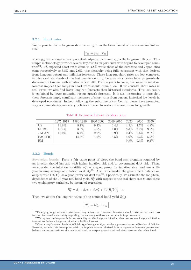
where g∞ is the long-run real potential output growth and π∞ is the long-run inflation. Thissimple methodology provides several key results, in particular with regard to developed coun-tries24. US expected short rates come to 4.8% while those of the eurozone and Japan onescome respectively to 3.8% and 2.6%, this hierarchy being fully consistent with that derivedfrom long-run output and inflation forecasts. These long-run short rates are low comparedto historical standards of the last quarter-century, because short rates have progressivelydecreased in tandem with inflation since 1980. For the years to come, our long-run inflationforecast implies that long-run short rates should remain low. If we consider short rates inreal terms, we also find lower long-run forecasts than historical standards. This last resultis explained by lower potential output growth forecasts. It is also interesting to note thatthese forecasts imply significant increases of short rates from current historical low levels indeveloped economies. Indeed, following the subprime crisis, Central banks have promotedvery accommodating monetary policies in order to restore the conditions for growth.
Table 3: Economic forecast for short rates
1975-1979 1980-1990 1990-2000 2000-2010 2020 2030 2050US 11.8% 8.7% 6.1% 6.4% 4.5% 4.7% 4.8%EURO 10.4% 8.0% 4.8% 4.0% 3.6% 3.7% 3.8%JAPAN 12.2% 6.4% 2.9% 0.9% 2.4% 2.5% 2.6%PACIFIC 14.5% 7.2% 5.5% 5.6% 5.3% 5.2%EM 9.8% 9.3% 9.1%
3.2.2 Bonds
Sovereign bonds From a fair value point of view, the bond risk premium required byan investor should increase with higher inflation risk and/or government debt risk. Then,we consider the inflation volatility σπt as a good proxy for inflation risk, and use a 10-year moving average of inflation volatility25. Also, we consider the government balance onoutput ratio (B/Y )t as a good proxy for debt risk26. Specifically, we estimate the long-termdependence of the 10-year real bond yield Rb
t with respect to the real short rate rt and thesetwo explanatory variables, by means of regression:
Rbt = β0 + β1rt + β2σ
πt + β3 (B/Y )t + εt
Then, we obtain the long-run value of the nominal bond yield Rb∞:
Rb∞ = Rb
∞ + π∞
24Emerging long-run short rates seem very attractive. However, investors should take into account twofactors: increased uncertainty regarding the currency outlook and economic improvements.
25We regress the long-run inflation volatility on the long-run inflation, then we use our long-run inflationforecast to derive a long-run inflation volatility forecast.
26Over a very long-run horizon, official organisms generally consider a progressive normalization of deficits.However, we mix this assumption with the implicit forecast derived from a regression between governmentbalance on output ratio on the one hand, and the output growth and real short rates on the other hand.
28
where the long-run real bond yield Rb∞ is obtained using the estimated regression model:
Rb∞ = β̂0 + β̂1r∞ + β̂2σ
π∞ + β̂3 (B/Y )∞
Remark 4 In order to facilitate the reading of this section, the numerical results of theregression models have been included in Appendix D.
Among the key conclusions derived from regression estimates, we pay attention to theeconomic interpretation of the results. Coefficients of real short rates are consistent with theeconomic intuition: real bond yields underreact to real short rate shifts. For illustration, a100 bps movement in the real short rate is associated with a 50 bps movement in the realbond yield on average, regardless of the geographic zone. Also, lower inflation volatilityand a higher government balance on output ratio are associated with a lower real bondyield. Finally, we find a positive coefficient β0, which is consistent with the existence of aliquidity risk premium. Our long-run forecasts exhibit interesting features. Indeed, we findthat US and eurozone bond yields stabilize between 4.8% and 5.1% at the 2050 horizon,which should be associated with an annualized return of 4.3% for the US and 4% for theeurozone, taking into account the trajectory of bond yields. These figures contrast with the9% annualized average performance posted since 198027, a period which was associated withstructural disinflation and decreasing inflation risk. Regarding contemporaneous low bondyields across the regions, our bond yield forecasts imply mixed performances for the horizon2010-2020.
Investment grade, high yield and emerging bonds We have chosen to regroup thesethree asset classes because their long-run returns are defined as the sum of the governmentbond return and a bond risk premium. As for government bonds, we propose to work witha bond yield, and then derive an expected return. We propose to analyze the differencescrt between the credit bond yield and the government bond yield, and to estimate therelationship with proxies for risk premium. For the investment grade and high yield spreads,we consider the following regression model:
scrt = β0 + β1σet + β2gt + εt
where σet denotes the equity volatility and gt is the output growth. For the emerging bondspread, the regression model becomes:
scrt = β0 + β1σet + β2 (CA/Y )t + εt
where (CA/Y )t is the current account on output ratio. Then again, we deduce the long-runspread scr∞ and the implied long-run bond yield Rcr
∞ using the relationship28:
Rcr∞ = Rb
∞ + scr∞
27Over a very long term, Dimson et al. (2010) find that bond excess returns over cash is about 1%on average, which is higher than our long-run forecasts, but lower than the 2% observed during the lastquarter-century.
28For the current account, we assume a null value at the horizon 2050, knowing that emerging economiestypically exhibit a positive current account as long as they converge to developed economies. For thevolatility, we consider long-run historical values, which are lower than those obtained during the two lastdecades, with the exception of the volatility of the emerging equity markets.
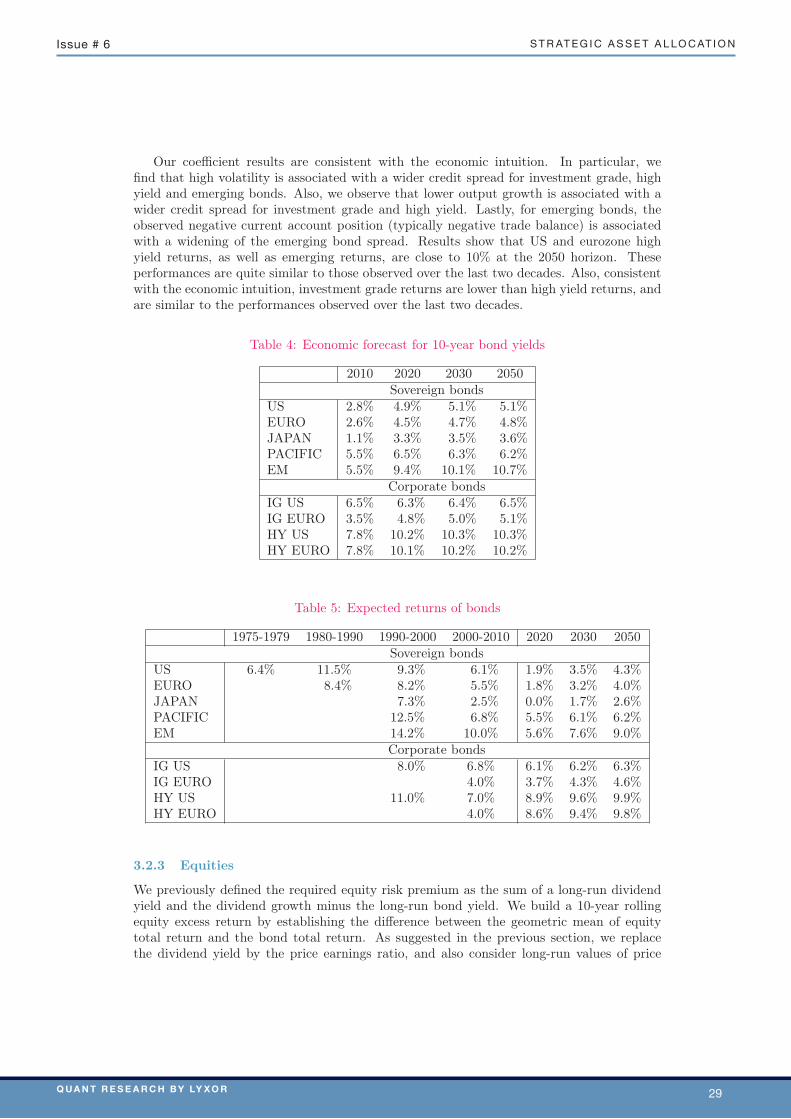
Q u a n t R e s e a R c h b y Ly x o R 29
s t r at e g i c a s s e t a l l o c at i o nissue # 6
Our coefficient results are consistent with the economic intuition. In particular, wefind that high volatility is associated with a wider credit spread for investment grade, highyield and emerging bonds. Also, we observe that lower output growth is associated with awider credit spread for investment grade and high yield. Lastly, for emerging bonds, theobserved negative current account position (typically negative trade balance) is associatedwith a widening of the emerging bond spread. Results show that US and eurozone highyield returns, as well as emerging returns, are close to 10% at the 2050 horizon. Theseperformances are quite similar to those observed over the last two decades. Also, consistentwith the economic intuition, investment grade returns are lower than high yield returns, andare similar to the performances observed over the last two decades.
Table 4: Economic forecast for 10-year bond yields
2010 2020 2030 2050Sovereign bonds
US 2.8% 4.9% 5.1% 5.1%EURO 2.6% 4.5% 4.7% 4.8%JAPAN 1.1% 3.3% 3.5% 3.6%PACIFIC 5.5% 6.5% 6.3% 6.2%EM 5.5% 9.4% 10.1% 10.7%
Corporate bondsIG US 6.5% 6.3% 6.4% 6.5%IG EURO 3.5% 4.8% 5.0% 5.1%HY US 7.8% 10.2% 10.3% 10.3%HY EURO 7.8% 10.1% 10.2% 10.2%
Table 5: Expected returns of bonds
1975-1979 1980-1990 1990-2000 2000-2010 2020 2030 2050Sovereign bonds
US 6.4% 11.5% 9.3% 6.1% 1.9% 3.5% 4.3%EURO 8.4% 8.2% 5.5% 1.8% 3.2% 4.0%JAPAN 7.3% 2.5% 0.0% 1.7% 2.6%PACIFIC 12.5% 6.8% 5.5% 6.1% 6.2%EM 14.2% 10.0% 5.6% 7.6% 9.0%
Corporate bondsIG US 8.0% 6.8% 6.1% 6.2% 6.3%IG EURO 4.0% 3.7% 4.3% 4.6%HY US 11.0% 7.0% 8.9% 9.6% 9.9%HY EURO 4.0% 8.6% 9.4% 9.8%
3.2.3 Equities
We previously defined the required equity risk premium as the sum of a long-run dividendyield and the dividend growth minus the long-run bond yield. We build a 10-year rollingequity excess return by establishing the difference between the geometric mean of equitytotal return and the bond total return. As suggested in the previous section, we replacethe dividend yield by the price earnings ratio, and also consider long-run values of price
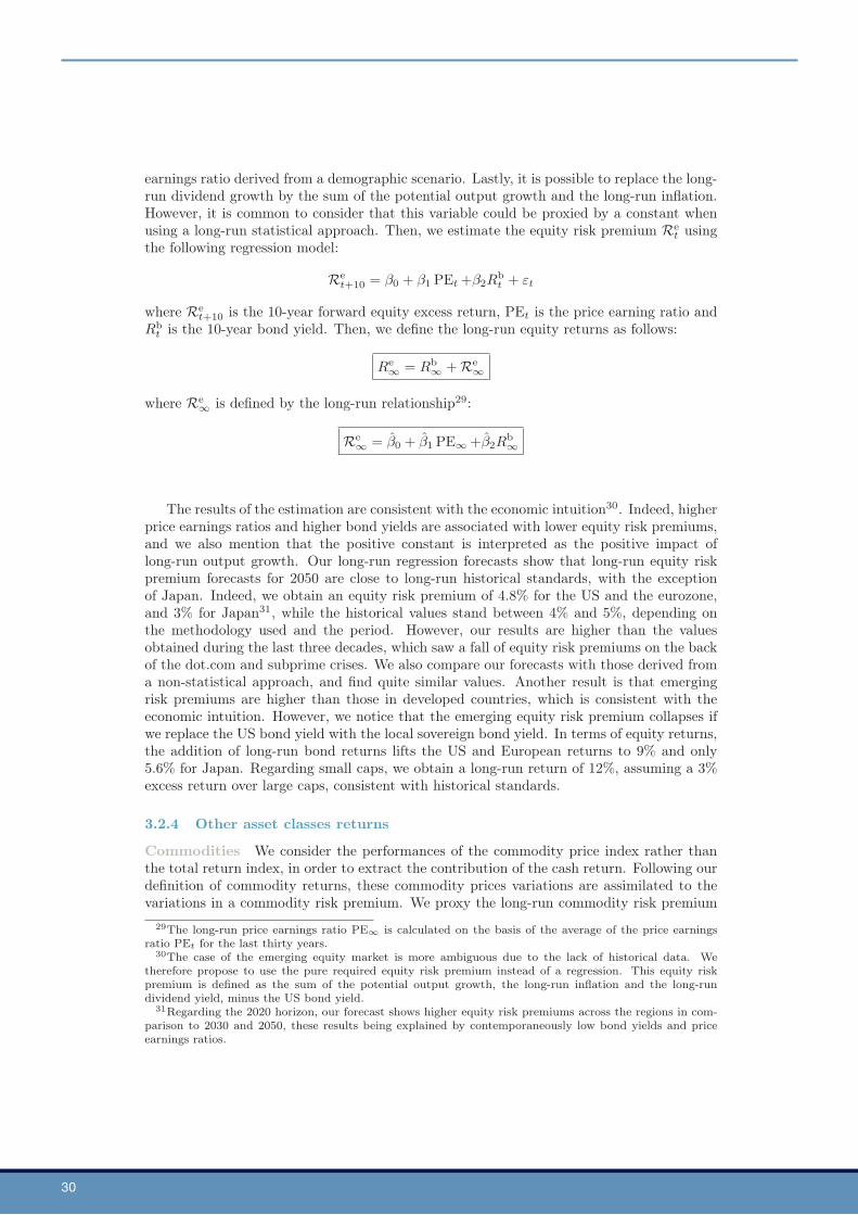
30
earnings ratio derived from a demographic scenario. Lastly, it is possible to replace the long-run dividend growth by the sum of the potential output growth and the long-run inflation.However, it is common to consider that this variable could be proxied by a constant whenusing a long-run statistical approach. Then, we estimate the equity risk premium Re
t usingthe following regression model:
Ret+10 = β0 + β1 PEt +β2R
bt + εt
where Ret+10 is the 10-year forward equity excess return, PEt is the price earning ratio and
Rbt is the 10-year bond yield. Then, we define the long-run equity returns as follows:
Re∞ = Rb
∞ +Re∞
where Re∞ is defined by the long-run relationship29:
Re∞ = β̂0 + β̂1 PE∞+β̂2R
b∞
The results of the estimation are consistent with the economic intuition30. Indeed, higherprice earnings ratios and higher bond yields are associated with lower equity risk premiums,and we also mention that the positive constant is interpreted as the positive impact oflong-run output growth. Our long-run regression forecasts show that long-run equity riskpremium forecasts for 2050 are close to long-run historical standards, with the exceptionof Japan. Indeed, we obtain an equity risk premium of 4.8% for the US and the eurozone,and 3% for Japan31, while the historical values stand between 4% and 5%, depending onthe methodology used and the period. However, our results are higher than the valuesobtained during the last three decades, which saw a fall of equity risk premiums on the backof the dot.com and subprime crises. We also compare our forecasts with those derived froma non-statistical approach, and find quite similar values. Another result is that emergingrisk premiums are higher than those in developed countries, which is consistent with theeconomic intuition. However, we notice that the emerging equity risk premium collapses ifwe replace the US bond yield with the local sovereign bond yield. In terms of equity returns,the addition of long-run bond returns lifts the US and European returns to 9% and only5.6% for Japan. Regarding small caps, we obtain a long-run return of 12%, assuming a 3%excess return over large caps, consistent with historical standards.
3.2.4 Other asset classes returns
Commodities We consider the performances of the commodity price index rather thanthe total return index, in order to extract the contribution of the cash return. Following ourdefinition of commodity returns, these commodity prices variations are assimilated to thevariations in a commodity risk premium. We proxy the long-run commodity risk premium
29The long-run price earnings ratio PE∞ is calculated on the basis of the average of the price earningsratio PEt for the last thirty years.
30The case of the emerging equity market is more ambiguous due to the lack of historical data. Wetherefore propose to use the pure required equity risk premium instead of a regression. This equity riskpremium is defined as the sum of the potential output growth, the long-run inflation and the long-rundividend yield, minus the US bond yield.
31Regarding the 2020 horizon, our forecast shows higher equity risk premiums across the regions in com-parison to 2030 and 2050, these results being explained by contemporaneously low bond yields and priceearnings ratios.
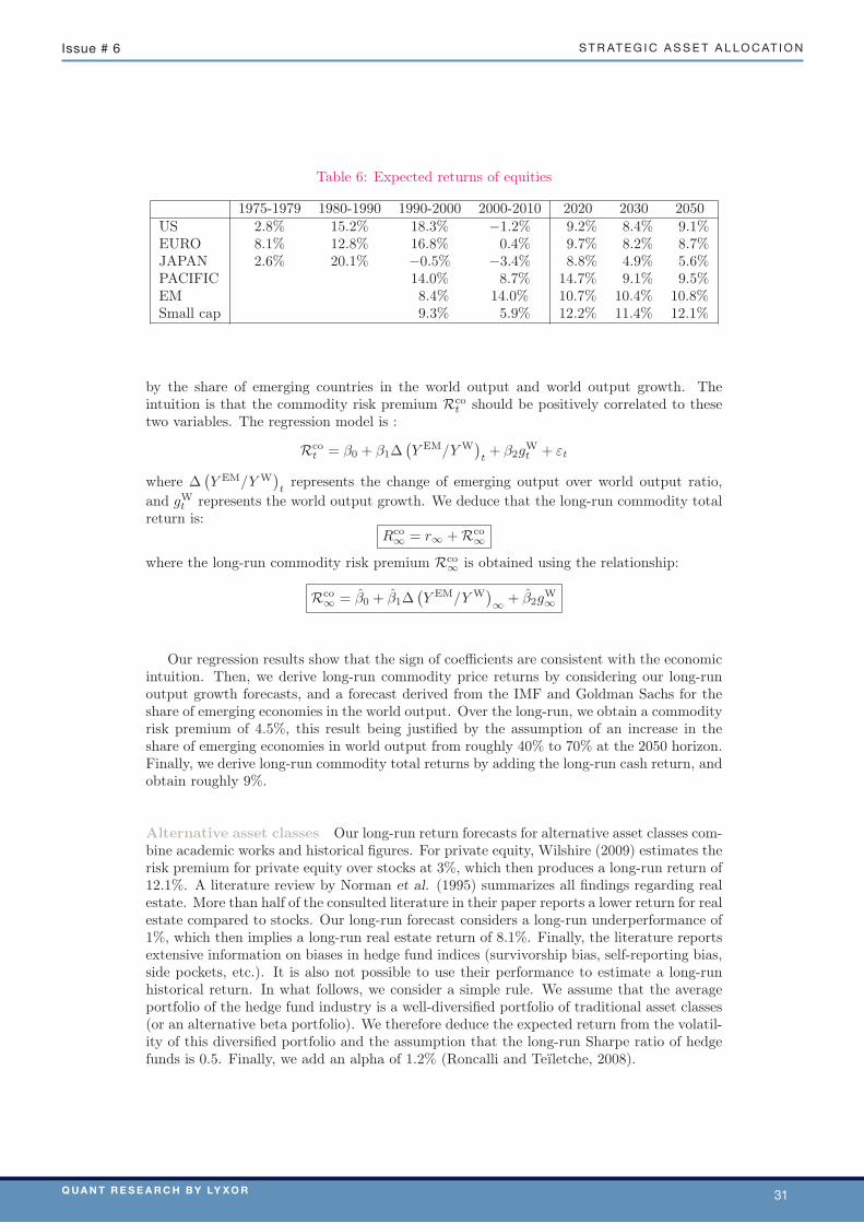
Q u a n t R e s e a R c h b y Ly x o R 31
s t r at e g i c a s s e t a l l o c at i o nissue # 6
Table 6: Expected returns of equities
1975-1979 1980-1990 1990-2000 2000-2010 2020 2030 2050US 2.8% 15.2% 18.3% −1.2% 9.2% 8.4% 9.1%EURO 8.1% 12.8% 16.8% 0.4% 9.7% 8.2% 8.7%JAPAN 2.6% 20.1% −0.5% −3.4% 8.8% 4.9% 5.6%PACIFIC 14.0% 8.7% 14.7% 9.1% 9.5%EM 8.4% 14.0% 10.7% 10.4% 10.8%Small cap 9.3% 5.9% 12.2% 11.4% 12.1%
by the share of emerging countries in the world output and world output growth. Theintuition is that the commodity risk premium Rco
t should be positively correlated to thesetwo variables. The regression model is :
Rcot = β0 + β1∆
Y EM/Y W
t+ β2g
Wt + εt
where ∆Y EM/Y W
t
represents the change of emerging output over world output ratio,and gW
t represents the world output growth. We deduce that the long-run commodity totalreturn is:
Rco∞ = r∞ +Rco
∞
where the long-run commodity risk premium Rco∞ is obtained using the relationship:
Rco∞ = β̂0 + β̂1∆
Y EM/Y W
∞ + β̂2g
W∞
Our regression results show that the sign of coefficients are consistent with the economicintuition. Then, we derive long-run commodity price returns by considering our long-runoutput growth forecasts, and a forecast derived from the IMF and Goldman Sachs for theshare of emerging economies in the world output. Over the long-run, we obtain a commodityrisk premium of 4.5%, this result being justified by the assumption of an increase in theshare of emerging economies in world output from roughly 40% to 70% at the 2050 horizon.Finally, we derive long-run commodity total returns by adding the long-run cash return, andobtain roughly 9%.
Alternative asset classes Our long-run return forecasts for alternative asset classes com-bine academic works and historical figures. For private equity, Wilshire (2009) estimates therisk premium for private equity over stocks at 3%, which then produces a long-run return of12.1%. A literature review by Norman et al. (1995) summarizes all findings regarding realestate. More than half of the consulted literature in their paper reports a lower return for realestate compared to stocks. Our long-run forecast considers a long-run underperformance of1%, which then implies a long-run real estate return of 8.1%. Finally, the literature reportsextensive information on biases in hedge fund indices (survivorship bias, self-reporting bias,side pockets, etc.). It is also not possible to use their performance to estimate a long-runhistorical return. In what follows, we consider a simple rule. We assume that the averageportfolio of the hedge fund industry is a well-diversified portfolio of traditional asset classes(or an alternative beta portfolio). We therefore deduce the expected return from the volatil-ity of this diversified portfolio and the assumption that the long-run Sharpe ratio of hedgefunds is 0.5. Finally, we add an alpha of 1.2% (Roncalli and Teïletche, 2008).
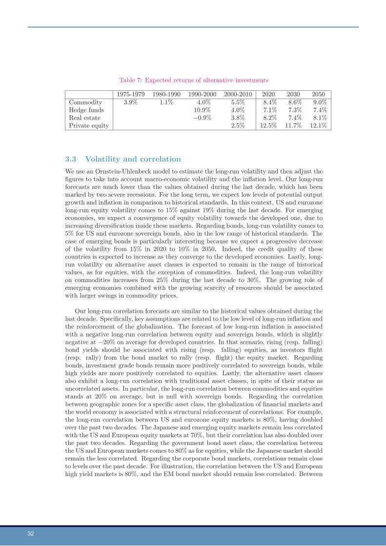
32
Table 7: Expected returns of alternative investments
1975-1979 1980-1990 1990-2000 2000-2010 2020 2030 2050Commodity 3.9% 1.1% 4.0% 5.5% 8.4% 8.6% 9.0%Hedge funds 10.9% 4.0% 7.1% 7.3% 7.4%Real estate −0.9% 3.8% 8.2% 7.4% 8.1%Private equity 2.5% 12.5% 11.7% 12.1%
3.3 Volatility and correlationWe use an Ornstein-Uhlenbeck model to estimate the long-run volatility and then adjust thefigures to take into account macro-economic volatility and the inflation level. Our long-runforecasts are much lower than the values obtained during the last decade, which has beenmarked by two severe recessions. For the long term, we expect low levels of potential outputgrowth and inflation in comparison to historical standards. In this context, US and eurozonelong-run equity volatility comes to 15% against 19% during the last decade. For emergingeconomies, we expect a convergence of equity volatility towards the developed one, due toincreasing diversification inside these markets. Regarding bonds, long-run volatility comes to5% for US and eurozone sovereign bonds, also in the low range of historical standards. Thecase of emerging bonds is particularly interesting because we expect a progressive decreaseof the volatility from 15% in 2020 to 10% in 2050. Indeed, the credit quality of thesecountries is expected to increase as they converge to the developed economies. Lastly, long-run volatility on alternative asset classes is expected to remain in the range of historicalvalues, as for equities, with the exception of commodities. Indeed, the long-run volatilityon commodities increases from 25% during the last decade to 30%. The growing role ofemerging economies combined with the growing scarcity of resources should be associatedwith larger swings in commodity prices.
Our long-run correlation forecasts are similar to the historical values obtained during thelast decade. Specifically, key assumptions are related to the low level of long-run inflation andthe reinforcement of the globalization. The forecast of low long-run inflation is associatedwith a negative long-run correlation between equity and sovereign bonds, which is slightlynegative at −20% on average for developed countries. In that scenario, rising (resp. falling)bond yields should be associated with rising (resp. falling) equities, as investors flight(resp. rally) from the bond market to rally (resp. flight) the equity market. Regardingbonds, investment grade bonds remain more positively correlated to sovereign bonds, whilehigh yields are more positively correlated to equities. Lastly, the alternative asset classesalso exhibit a long-run correlation with traditional asset classes, in spite of their status asuncorrelated assets. In particular, the long-run correlation between commodities and equitiesstands at 20% on average, but is null with sovereign bonds. Regarding the correlationbetween geographic zones for a specific asset class, the globalization of financial markets andthe world economy is associated with a structural reinforcement of correlations. For example,the long-run correlation between US and eurozone equity markets is 80%, having doubledover the past two decades. The Japanese and emerging equity markets remain less correlatedwith the US and European equity markets at 70%, but their correlation has also doubled overthe past two decades. Regarding the government bond asset class, the correlation betweenthe US and European markets comes to 80% as for equities, while the Japanese market shouldremain the less correlated. Regarding the corporate bond markets, correlations remain closeto levels over the past decade. For illustration, the correlation between the US and Europeanhigh yield markets is 80%, and the EM bond market should remain less correlated. Between
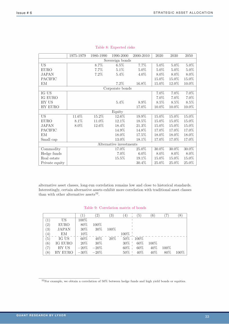
Q u a n t R e s e a R c h b y Ly x o R 33
s t r at e g i c a s s e t a l l o c at i o nissue # 6
Table 8: Expected risks
1975-1979 1980-1990 1990-2000 2000-2010 2020 2030 2050Sovereign bonds
US 8.7% 6.5% 7.7% 5.0% 5.0% 5.0%EURO 7.7% 5.1% 5.0% 5.0% 5.0% 5.0%JAPAN 7.2% 5.4% 4.0% 8.0% 8.0% 8.0%PACIFIC 15.0% 15.0% 15.0%EM 7.2% 16.8% 15.0% 12.0% 10.0%
Corporate bondsIG US 7.0% 7.0% 7.0%IG EURO 7.0% 7.0% 7.0%HY US 5.4% 8.9% 8.5% 8.5% 8.5%HY EURO 17.0% 10.0% 10.0% 10.0%
EquityUS 11.6% 15.2% 12.6% 19.9% 15.0% 15.0% 15.0%EURO 8.1% 11.0% 12.1% 18.5% 15.0% 15.0% 15.0%JAPAN 8.0% 12.6% 18.4% 21.3% 15.0% 15.0% 15.0%PACIFIC 14.9% 14.8% 17.0% 17.0% 17.0%EM 18.0% 17.5% 18.0% 18.0% 18.0%Small cap 13.0% 18.1% 17.0% 17.0% 17.0%
Alternative investmentsCommodity 17.0% 25.0% 30.0% 30.0% 30.0%Hedge funds 7.0% 6.0% 8.0% 8.0% 8.0%Real estate 15.5% 19.1% 15.0% 15.0% 15.0%Private equity 30.4% 25.0% 25.0% 25.0%
alternative asset classes, long-run correlation remains low and close to historical standards.Interestingly, certain alternative assets exhibit more correlation with traditional asset classesthan with other alternative assets32.
Table 9: Correlation matrix of bonds
(1) (2) (3) (4) (5) (6) (7) (8)(1) US 100%(2) EURO 80% 100%(3) JAPAN 30% 30% 100%(4) EM 10% 100%(5) IG US 60% 40% 20% 50% 100%(6) IG EURO 20% 30% 30% 60% 100%(7) HY US −20% −20% 60% 60% 40% 100%(8) HY EURO −30% −20% 50% 40% 40% 80% 100%
32For example, we obtain a correlation of 50% between hedge funds and high yield bonds or equities.
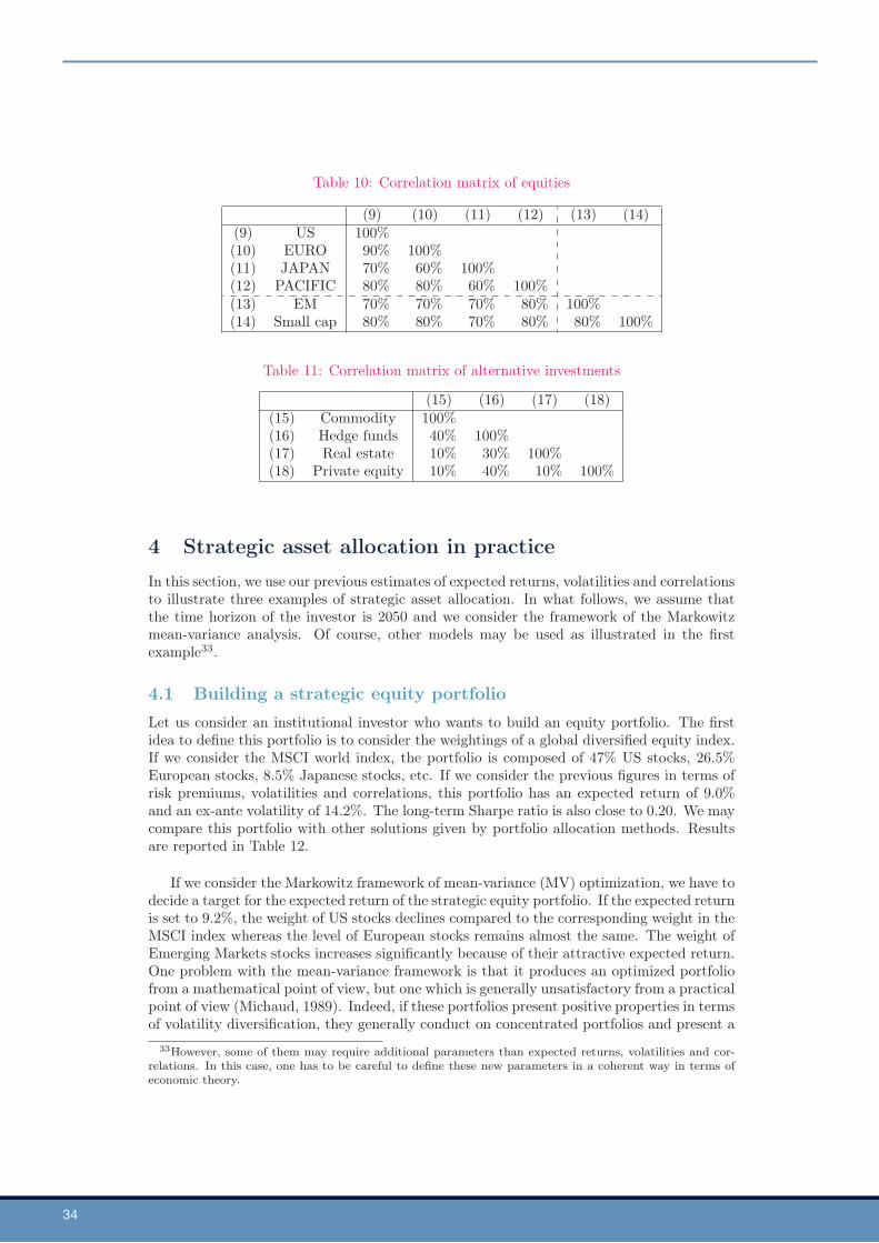
34
Table 10: Correlation matrix of equities
(9) (10) (11) (12) (13) (14)(9) US 100%(10) EURO 90% 100%(11) JAPAN 70% 60% 100%(12) PACIFIC 80% 80% 60% 100%(13) EM 70% 70% 70% 80% 100%(14) Small cap 80% 80% 70% 80% 80% 100%
Table 11: Correlation matrix of alternative investments
(15) (16) (17) (18)(15) Commodity 100%(16) Hedge funds 40% 100%(17) Real estate 10% 30% 100%(18) Private equity 10% 40% 10% 100%
4 Strategic asset allocation in practice
In this section, we use our previous estimates of expected returns, volatilities and correlationsto illustrate three examples of strategic asset allocation. In what follows, we assume thatthe time horizon of the investor is 2050 and we consider the framework of the Markowitzmean-variance analysis. Of course, other models may be used as illustrated in the firstexample33.
4.1 Building a strategic equity portfolio
Let us consider an institutional investor who wants to build an equity portfolio. The firstidea to define this portfolio is to consider the weightings of a global diversified equity index.If we consider the MSCI world index, the portfolio is composed of 47% US stocks, 26.5%European stocks, 8.5% Japanese stocks, etc. If we consider the previous figures in terms ofrisk premiums, volatilities and correlations, this portfolio has an expected return of 9.0%and an ex-ante volatility of 14.2%. The long-term Sharpe ratio is also close to 0.20. We maycompare this portfolio with other solutions given by portfolio allocation methods. Resultsare reported in Table 12.
If we consider the Markowitz framework of mean-variance (MV) optimization, we have todecide a target for the expected return of the strategic equity portfolio. If the expected returnis set to 9.2%, the weight of US stocks declines compared to the corresponding weight in theMSCI index whereas the level of European stocks remains almost the same. The weight ofEmerging Markets stocks increases significantly because of their attractive expected return.One problem with the mean-variance framework is that it produces an optimized portfoliofrom a mathematical point of view, but one which is generally unsatisfactory from a practicalpoint of view (Michaud, 1989). Indeed, if these portfolios present positive properties in termsof volatility diversification, they generally conduct on concentrated portfolios and present a
33However, some of them may require additional parameters than expected returns, volatilities and cor-relations. In this case, one has to be careful to define these new parameters in a coherent way in terms ofeconomic theory.
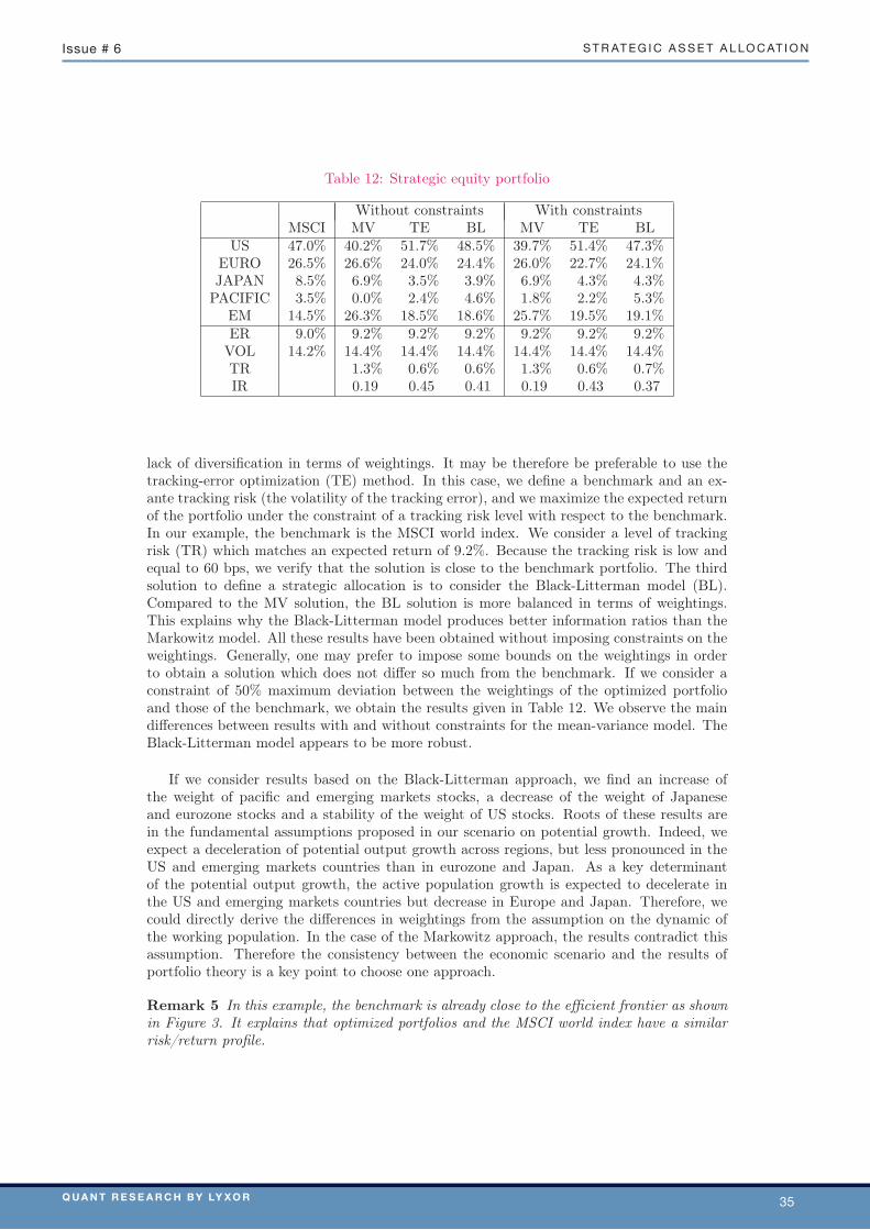
Q u a n t R e s e a R c h b y Ly x o R 35
s t r at e g i c a s s e t a l l o c at i o nissue # 6
Table 12: Strategic equity portfolio
Without constraints With constraintsMSCI MV TE BL MV TE BL
US 47.0% 40.2% 51.7% 48.5% 39.7% 51.4% 47.3%EURO 26.5% 26.6% 24.0% 24.4% 26.0% 22.7% 24.1%JAPAN 8.5% 6.9% 3.5% 3.9% 6.9% 4.3% 4.3%
PACIFIC 3.5% 0.0% 2.4% 4.6% 1.8% 2.2% 5.3%EM 14.5% 26.3% 18.5% 18.6% 25.7% 19.5% 19.1%ER 9.0% 9.2% 9.2% 9.2% 9.2% 9.2% 9.2%
VOL 14.2% 14.4% 14.4% 14.4% 14.4% 14.4% 14.4%TR 1.3% 0.6% 0.6% 1.3% 0.6% 0.7%IR 0.19 0.45 0.41 0.19 0.43 0.37
lack of diversification in terms of weightings. It may be therefore be preferable to use thetracking-error optimization (TE) method. In this case, we define a benchmark and an ex-ante tracking risk (the volatility of the tracking error), and we maximize the expected returnof the portfolio under the constraint of a tracking risk level with respect to the benchmark.In our example, the benchmark is the MSCI world index. We consider a level of trackingrisk (TR) which matches an expected return of 9.2%. Because the tracking risk is low andequal to 60 bps, we verify that the solution is close to the benchmark portfolio. The thirdsolution to define a strategic allocation is to consider the Black-Litterman model (BL).Compared to the MV solution, the BL solution is more balanced in terms of weightings.This explains why the Black-Litterman model produces better information ratios than theMarkowitz model. All these results have been obtained without imposing constraints on theweightings. Generally, one may prefer to impose some bounds on the weightings in orderto obtain a solution which does not differ so much from the benchmark. If we consider aconstraint of 50% maximum deviation between the weightings of the optimized portfolioand those of the benchmark, we obtain the results given in Table 12. We observe the maindifferences between results with and without constraints for the mean-variance model. TheBlack-Litterman model appears to be more robust.
If we consider results based on the Black-Litterman approach, we find an increase ofthe weight of pacific and emerging markets stocks, a decrease of the weight of Japaneseand eurozone stocks and a stability of the weight of US stocks. Roots of these results arein the fundamental assumptions proposed in our scenario on potential growth. Indeed, weexpect a deceleration of potential output growth across regions, but less pronounced in theUS and emerging markets countries than in eurozone and Japan. As a key determinantof the potential output growth, the active population growth is expected to decelerate inthe US and emerging markets countries but decrease in Europe and Japan. Therefore, wecould directly derive the differences in weightings from the assumption on the dynamic ofthe working population. In the case of the Markowitz approach, the results contradict thisassumption. Therefore the consistency between the economic scenario and the results ofportfolio theory is a key point to choose one approach.
Remark 5 In this example, the benchmark is already close to the efficient frontier as shownin Figure 3. It explains that optimized portfolios and the MSCI world index have a similarrisk/return profile.
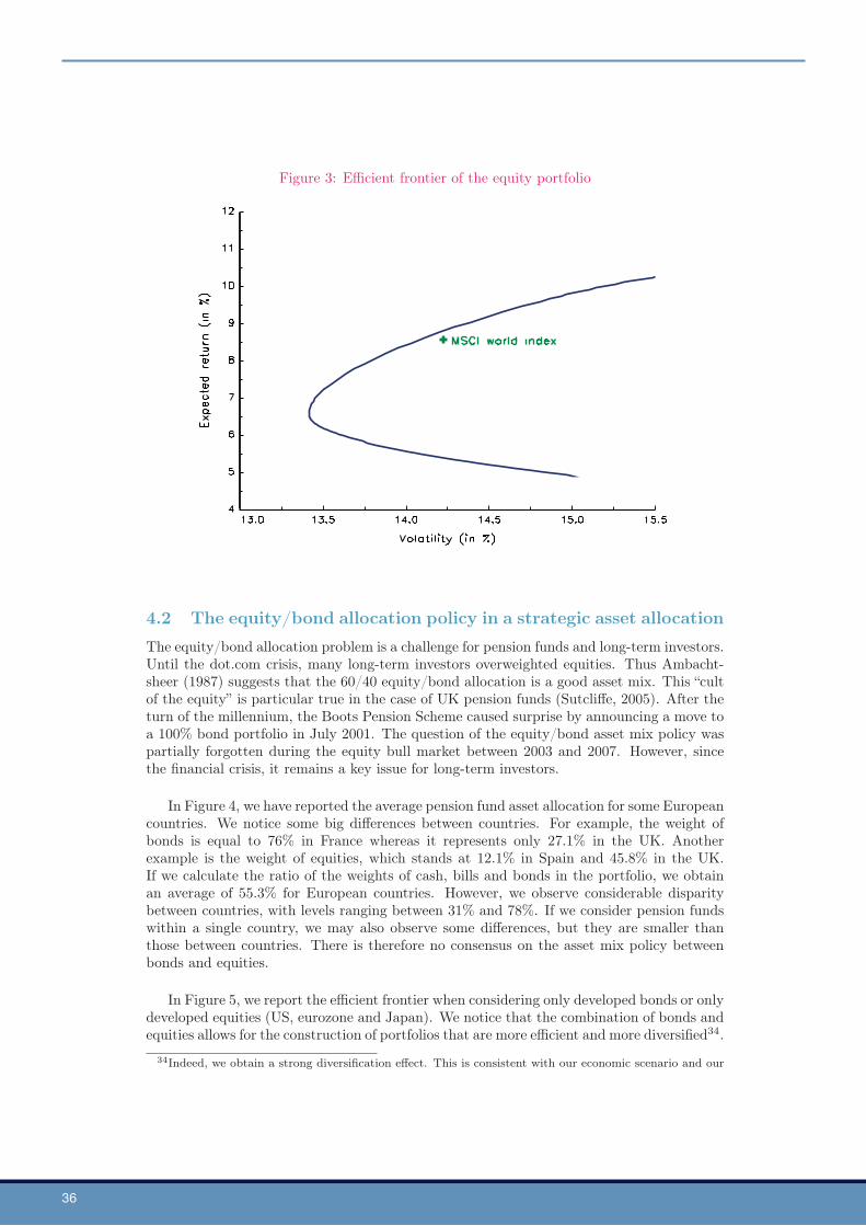
36
Figure 3: Efficient frontier of the equity portfolio
4.2 The equity/bond allocation policy in a strategic asset allocation
The equity/bond allocation problem is a challenge for pension funds and long-term investors.Until the dot.com crisis, many long-term investors overweighted equities. Thus Ambacht-sheer (1987) suggests that the 60/40 equity/bond allocation is a good asset mix. This “cultof the equity” is particular true in the case of UK pension funds (Sutcliffe, 2005). After theturn of the millennium, the Boots Pension Scheme caused surprise by announcing a move toa 100% bond portfolio in July 2001. The question of the equity/bond asset mix policy waspartially forgotten during the equity bull market between 2003 and 2007. However, sincethe financial crisis, it remains a key issue for long-term investors.
In Figure 4, we have reported the average pension fund asset allocation for some Europeancountries. We notice some big differences between countries. For example, the weight ofbonds is equal to 76% in France whereas it represents only 27.1% in the UK. Anotherexample is the weight of equities, which stands at 12.1% in Spain and 45.8% in the UK.If we calculate the ratio of the weights of cash, bills and bonds in the portfolio, we obtainan average of 55.3% for European countries. However, we observe considerable disparitybetween countries, with levels ranging between 31% and 78%. If we consider pension fundswithin a single country, we may also observe some differences, but they are smaller thanthose between countries. There is therefore no consensus on the asset mix policy betweenbonds and equities.
In Figure 5, we report the efficient frontier when considering only developed bonds or onlydeveloped equities (US, eurozone and Japan). We notice that the combination of bonds andequities allows for the construction of portfolios that are more efficient and more diversified34.
34Indeed, we obtain a strong diversification effect. This is consistent with our economic scenario and our
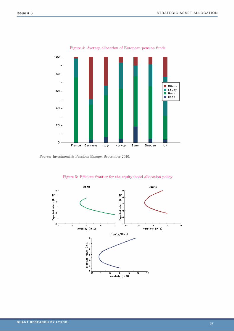
Q u a n t R e s e a R c h b y Ly x o R 37
s t r at e g i c a s s e t a l l o c at i o nissue # 6
Figure 4: Average allocation of European pension funds
Source: Investment & Pensions Europe, September 2010.
Figure 5: Efficient frontier for the equity/bond allocation policy
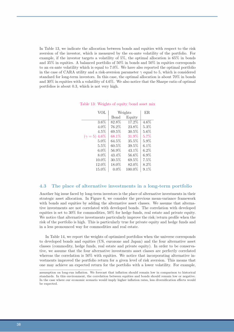
38
In Table 13, we indicate the allocation between bonds and equities with respect to the riskaversion of the investor, which is measured by the ex-ante volatility of the portfolio. Forexample, if the investor targets a volatility of 5%, the optimal allocation is 65% in bondsand 35% in equities. A balanced portfolio of 50% in bonds and 50% in equities correspondsto an ex-ante volatility which is equal to 7.0%. We have also reported the optimal portfolioin the case of CARA utility and a risk-aversion parameter γ equal to 5, which is consideredstandard for long-term investors. In this case, the optimal allocation is about 70% in bondsand 30% in equities with a volatility of 4.6%. We also notice that the Sharpe ratio of optimalportfolios is about 0.3, which is not very high.
Table 13: Weights of equity/bond asset mix
VOL Weights ERBond Equity
3.6% 82.8% 17.2% 4.6%4.0% 76.2% 23.8% 5.3%4.5% 69.5% 30.5% 5.6%
(γ = 5) 4.6% 68.1% 31.9% 5.7%5.0% 64.5% 35.5% 5.9%5.5% 60.5% 39.5% 6.1%6.0% 56.9% 43.1% 6.2%8.0% 43.4% 56.6% 6.9%10.0% 30.5% 69.5% 7.5%12.0% 18.0% 82.0% 8.2%15.0% 0.0% 100.0% 9.1%
4.3 The place of alternative investments in a long-term portfolio
Another big issue faced by long-term investors is the place of alternative investments in theirstrategic asset allocation. In Figure 6, we consider the previous mean-variance frameworkwith bonds and equities by adding the alternative asset classes. We assume that alterna-tive investments are not correlated with developed bonds. The correlation with developedequities is set to 30% for commodities, 50% for hedge funds, real estate and private equity.We notice that alternative investments particularly improve the risk/return profile when therisk of the portfolio is high. This is particularly true for private equity and hedge funds andin a less pronounced way for commodities and real estate.
In Table 14, we report the weights of optimized portfolios when the universe correspondsto developed bonds and equities (US, eurozone and Japan) and the four alternative assetclasses (commodity, hedge funds, real estate and private equity). In order to be conserva-tive, we assume that the four alternative investments asset classes are perfectly correlatedwhereas the correlation is 50% with equities. We notice that incorporating alternative in-vestments improved the portfolio return for a given level of risk aversion. This means thatone may achieve an expected return for the portfolio with a lower volatility. For example,
assumption on long-run inflation. We forecast that inflation should remain low in comparison to historicalstandards. In this environment, the correlation between equities and bonds should remain low or negative.In the case where our economic scenario would imply higher inflation rates, less diversification effects wouldbe expected.
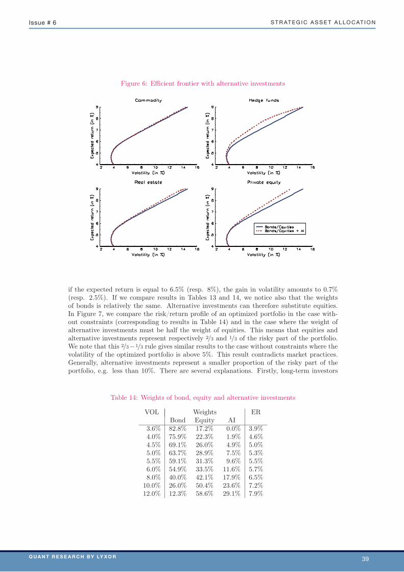
Q u a n t R e s e a R c h b y Ly x o R 39
s t r at e g i c a s s e t a l l o c at i o nissue # 6
Figure 6: Efficient frontier with alternative investments
if the expected return is equal to 6.5% (resp. 8%), the gain in volatility amounts to 0.7%(resp. 2.5%). If we compare results in Tables 13 and 14, we notice also that the weightsof bonds is relatively the same. Alternative investments can therefore substitute equities.In Figure 7, we compare the risk/return profile of an optimized portfolio in the case with-out constraints (corresponding to results in Table 14) and in the case where the weight ofalternative investments must be half the weight of equities. This means that equities andalternative investments represent respectively 2/3 and 1/3 of the risky part of the portfolio.We note that this 2/3−1/3 rule gives similar results to the case without constraints where thevolatility of the optimized portfolio is above 5%. This result contradicts market practices.Generally, alternative investments represent a smaller proportion of the risky part of theportfolio, e.g. less than 10%. There are several explanations. Firstly, long-term investors
Table 14: Weights of bond, equity and alternative investments
VOL Weights ERBond Equity AI
3.6% 82.8% 17.2% 0.0% 3.9%4.0% 75.9% 22.3% 1.9% 4.6%4.5% 69.1% 26.0% 4.9% 5.0%5.0% 63.7% 28.9% 7.5% 5.3%5.5% 59.1% 31.3% 9.6% 5.5%6.0% 54.9% 33.5% 11.6% 5.7%8.0% 40.0% 42.1% 17.9% 6.5%
10.0% 26.0% 50.4% 23.6% 7.2%12.0% 12.3% 58.6% 29.1% 7.9%
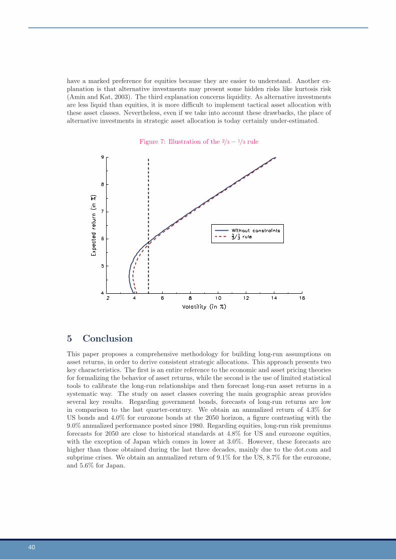
40
have a marked preference for equities because they are easier to understand. Another ex-planation is that alternative investments may present some hidden risks like kurtosis risk(Amin and Kat, 2003). The third explanation concerns liquidity. As alternative investmentsare less liquid than equities, it is more difficult to implement tactical asset allocation withthese asset classes. Nevertheless, even if we take into account these drawbacks, the place ofalternative investments in strategic asset allocation is today certainly under-estimated.
Figure 7: Illustration of the 2/3− 1/3 rule
5 ConclusionThis paper proposes a comprehensive methodology for building long-run assumptions onasset returns, in order to derive consistent strategic allocations. This approach presents twokey characteristics. The first is an entire reference to the economic and asset pricing theoriesfor formalizing the behavior of asset returns, while the second is the use of limited statisticaltools to calibrate the long-run relationships and then forecast long-run asset returns in asystematic way. The study on asset classes covering the main geographic areas providesseveral key results. Regarding government bonds, forecasts of long-run returns are lowin comparison to the last quarter-century. We obtain an annualized return of 4.3% forUS bonds and 4.0% for eurozone bonds at the 2050 horizon, a figure contrasting with the9.0% annualized performance posted since 1980. Regarding equities, long-run risk premiumsforecasts for 2050 are close to historical standards at 4.8% for US and eurozone equities,with the exception of Japan which comes in lower at 3.0%. However, these forecasts arehigher than those obtained during the last three decades, mainly due to the dot.com andsubprime crises. We obtain an annualized return of 9.1% for the US, 8.7% for the eurozone,and 5.6% for Japan.
Q u a n t R e s e a R c h b y Ly x o R 41
s t r at e g i c a s s e t a l l o c at i o nissue # 6
Then, we illustrate strategic allocations derived from our long-run asset returns forecasts,subject to different optimizing methodologies and different risk targets. In particular, webegin by considering the case of a pure equity portfolio, then we work on an equity/bondportfolio, and finally question the place of alternative investments. We conclude from thisanalysis that the equity/bond asset mix in a strategic portfolio is still a widely debatedtopic, with proportions differing greatly between countries, especially in Europe. We showthat institutional investors sometimes appear myopic, forgetting this asset mix questionduring the 2003-2007 equity bull market, and then reconsidering it as a key element afterthe recent financial crisis. Regarding the place of alternative investments, we also find thatallocations probably remain under-estimated, although this can be explained by inherentrisks associated with these investment vehicles.
An important question that arises nowadays is the choice of the relevant horizons for themain investment decisions in a strategic portfolio. Indeed, long-term investors are probablyconfused about the definition of strategic and tactical asset allocations. Most of them,willing to tackle the issue of the large swings on the financial markets during the recentcrisis, decided to reduce the horizon for their strategic allocation revisions and to implementshort-term money management on a small part of their portfolios, which they call tacticalallocations. We think that this framework is not consistent with economic theory. There isstill a need for a strategic portfolio that is designed to be consistent with the long-term pathof the economy. This should not be revised unless major structural breaks in the economyoccur, like productivity shocks or changes in demography or monetary policy. By definition,relevant horizons for such investments are much longer than the business cycle. Nevertheless,there is still room for the implementation of a dynamic asset allocation. Merton (1973) andLucas (1978) paved the way for this by showing that risk premiums vary over time35. Overthe past two decades, Barberis (2000) and Campbell and Viceira (2002) among others,showed in which proportions asset weights should change in accordance with time-varyingrisk premiums. Then, from our point of view, tactical asset allocation is justifiable as long asit is designed to hedge against unwanted variations of the economic cycle. This means thatthe tactical investment horizons range from a few months to two or three years. All othershorter-term bets in the portfolio should be considered as a way to time the market. Then,we could imagine a hybrid investment policy for long-term investors, where the strategicallocation could be obtained as a reference portfolio, while the tactical allocation wouldjustify adjustments of this reference portfolio within the business cycle. In this framework,confusions between market timing and tactical asset allocation are avoided36.
35See Darolles et al. (2010) for a survey on the subject.36This does not exclude market timing from a long-term investment policy. It only means that TAA is
fundamentally an economic asset allocation.

42
A NotationsTable 15 describes the different variables used in this paper. Let Xt be an economic orfinancial variable. The corresponding long-run steady state or value will be denoted by X∞.In order to distinguish nominal and real (or excess) returns, we use a calligraphic symbol forthe real return. Parameters used in the different models are in lowercase whereas coefficientsof regression models are denoted by the Greek letter β and estimates correspond to β̂.
Table 15: Notation and description of the economic and financial variables
Notation Description Formulaπt Inflationgt Output growthσπt Inflation volatilityYt OutputCt ConsumptionIt Investment It = Yt − CtKt CapitalLt Labor force(B/Y )t Ratio of the government balance on output(CA/Y )t Ratio of the current account on outputrt Short-term interest ratert Real interest rate rt = rt − πt
R(m)t Interest rate of maturity m
St Spot exchange rateF
(m)t Forward exchange rate of maturity m
Rbt Nominal sovereign bond yieldRbt Real sovereign bond yield Rb
t = Rbt − πt
Rcrt Nominal credit bond yield
scrt Credit bond spread scrt = Rcrt −Rb
t
Ret Equity returnRet Equity excess return Re
t = Ret −Rb
t
Rcot Commodity total returnRcot Commodity excess return Rco
t = Rcot − rt
σet Volatility of equity returns
Pt PriceDt DividendDYt Dividend yield DYt = Dt+1/PtPEt Price earnings ratio
Q u a n t R e s e a R c h b y Ly x o R 43
s t r at e g i c a s s e t a l l o c at i o nissue # 6
B Macro-economics pillars
B.1 Modeling economic growth
B.1.1 The Solow growth model
In its original form, the Solow model is a pure production model of a closed economy wherethe output Yt is a production function depending on capital, labor and technology. Thisfunction is assumed to exhibit constant returns to scale (CRTS) and decreasing marginalproductivity of capital. The model attempts to capture the dynamics of economic growth,stating that it converges to an equilibrium where the determinants that create additions tocapital and those that make capital decrease exactly offset each other. The only endogenousvariable of the model is the capital Kt. This means that variations of the output are relatedonly to endogenous variations of capital. The working population is represented by the laborforce Lt and productivity gains are due to some technological progress At. Solow (1956)assumes that these two exogenous variables grow at constant rates η and γ. He does notassume any model for the consumer. All the consumers own all the firms, their income isprovided by the output of the firms, and the proportion of output that is not consumed isre-invested in the firms next period.
Thus, we have:Yt = F (Kt, AtLt)
where AtLt represents the effective labor and F is the production function. Given the CRTScondition, we can write:
Yt
AtLt= F
Kt
AtLt, 1
= f
Kt
AtLt
We denote yt = Yt/ (AtLt) and kt = Kt/ (AtLt) respectively the output per effective workerand capital per effective worker. Then, the model relies on the following equations.
1. The production function implies that, at any time, output per effective worker dependsonly on capital per effective worker37:
yt = f (kt)
2. We assume that the investment It which is defined by the difference between the outputYt and the consumptions Ct is a constant proportion of the output Yt:
It = Yt − Ct = sYt
with s denoting the savings rate. The rule of accumulation of capital then drives thedynamics of the capital:
dKt
dt= It − δKt
where δ is the constant rate of capital depreciation.
37It is also assumed that f (0) = 0, f (k) > 0, f (k) < 0. This last condition ensures that the marginalproductivity of capital is decreasing. Finally, the function f is defined so that it verifies Inada conditions,that is limk→0 f (k) = +∞ and limk→+∞ f (k) = 0.
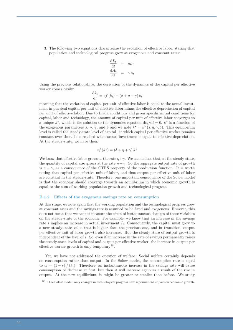
44
3. The following two equations characterize the evolution of effective labor, stating thatpopulation and technological progress grow at exogenous and constant rates:
dLt
dt= ηLt
dAt
dt= γAt
Using the previous relationships, the derivation of the dynamics of the capital per effectiveworker comes easily:
dkt
dt= sf (kt)− (δ + η + γ) kt
meaning that the variation of capital per unit of effective labor is equal to the actual invest-ment in physical capital per unit of effective labor minus the effective depreciation of capitalper unit of effective labor. Due to Inada conditions and given specific initial conditions forcapital, labor and technology, the amount of capital per unit of effective labor converges toa unique k, which is the solution to the dynamics equation dkt/dt = 0. k∗ is a function ofthe exogenous parameters s, η, γ, and δ and we note k = k∗ (s, η, γ, δ). This equilibriumlevel is called the steady-state level of capital, at which capital per effective worker remainsconstant over time. It is reached when actual investment is equal to effective depreciation.At the steady-state, we have then:
sf (k) = (δ + η + γ) k
We know that effective labor grows at the rate η+γ. We can deduce that, at the steady-state,the quantity of capital also grows at the rate η+ γ. So the aggregate output rate of growthis η + γ, as a consequence of the CTRS property of the production function. It is worthnoting that capital per effective unit of labor, and thus output per effective unit of laborare constant in the steady-state. Therefore, one important consequence of the Solow modelis that the economy should converge towards an equilibrium in which economic growth isequal to the sum of working population growth and technological progress.
B.1.2 Effects of the exogenous savings rate on consumption
At this stage, we note again that the working population and the technological progress growat constant rates and the savings rate is assumed to be fixed and exogenous. However, thisdoes not mean that we cannot measure the effect of instantaneous changes of these variableson the steady-state of the economy. For example, we know that an increase in the savingsrate s implies an increase in actual investment It. Consequently, the capital must grow toa new steady-state value that is higher than the previous one, and in transition, outputper effective unit of labor growth also increases. But the steady-state of output growth isindependent of the level of s. So, even if an increase in the rate of savings permanently raisesthe steady-state levels of capital and output per effective worker, the increase in output pereffective worker growth is only temporary38.
Yet, we have not addressed the question of welfare. Social welfare certainly dependson consumption rather than output. In the Solow model, the consumption rate is equalto ct = (1− s) f (kt). Therefore, an instantaneous increase in the savings rate will causeconsumption to decrease at first, but then it will increase again as a result of the rise inoutput. At the new equilibrium, it might be greater or smaller than before. We study
38In the Solow model, only changes in technological progress have a permanent impact on economic growth.

Q u a n t R e s e a R c h b y Ly x o R 45
s t r at e g i c a s s e t a l l o c at i o nissue # 6
the effect of changes in the savings rate on consumption at the steady-state, by derivingconsumption in the steady-state c with respect to s. We have c = f (k)− (δ + η + γ) k
and ∂sc = (f (k)− (δ + η + γ)) · ∂sk
. We know that ∂sk > 0. Also, from Inada
conditions, the quantity f (k)− (δ + η + γ) is positive for small values of k and negativefor large values of k. Thus, everything else being equal, steady-state consumption admitsa maximum with respect to the savings rate, which is the solution to ∂sc
= 0. The highestpossible level of consumption in the steady-state is also attained at f (k)− δ = η + γ. Atequilibrium, consumption per effective unit of labor is at a maximum when the marginalproduct of capital net of depreciation is equal to the growth rate of of the economy.
B.1.3 The Golden Rule of capital accumulation
Historically, the term Golden Rule is an ethical code that is a base concept of human rightsand that can be formulated as follows:
“Treat others according to how you would like others to treat you”.
Applied to our economic context, the terms “you” and “others” refer to the actual andthe next generation respectively. The underlying idea is that if we (more precisely, the“government”) are concerned about social welfare, how should we act so that ours is identicalto the next generations? Probably, by maximizing consumption per capita at the equilibriumof the economy. We introduce the quantity et = ∂kyt/ (yt/kt) which measures the elasticityof the output with respect to the capital. In the steady-state, we have:
e =s
δ + η + γm
where m = f (k) is the marginal product of capital. Thus, the savings rate that thegovernment should try to attain is the one that maximizes consumption in the steady-state,and hence, is equal to e. How does this relate to the financial assets rate of return? Inthe neo-classical theory of production, the level of production depends only on the supply ofgoods in the context of pure and perfect competition. Then the producer tries to maximizehis profit Π = Py−Rk where P and R denote respectively the price of output and the costof capital, under the constraint y = f (k). The first-order condition is ∂kf (k) = R/P , whichmeans that the marginal product of capital is equal to the real cost of capital (denoted r):
m = r
From an investor’s point of view, it is exactly the minimum expected return for an investmentto be worthwhile. As such, it can be thought of as the required risk-free rate for financialassets’ risk premium evaluation. At the steady-state, we have then:
r − e
sδ =
e
s(η + γ)
Finally, applying the Solow model and according to the Golden Rule e = s, the financialmarkets’ risk-free rate net of depreciation of capital r = rc − δ should be equal to the realrate of growth g of the economy at equilibrium:
r = g = η + γ
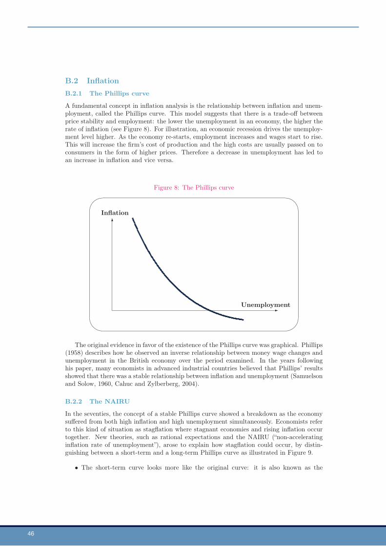
46
B.2 Inflation
B.2.1 The Phillips curve
A fundamental concept in inflation analysis is the relationship between inflation and unem-ployment, called the Phillips curve. This model suggests that there is a trade-off betweenprice stability and employment: the lower the unemployment in an economy, the higher therate of inflation (see Figure 8). For illustration, an economic recession drives the unemploy-ment level higher. As the economy re-starts, employment increases and wages start to rise.This will increase the firm’s cost of production and the high costs are usually passed on toconsumers in the form of higher prices. Therefore a decrease in unemployment has led toan increase in inflation and vice versa.
Figure 8: The Phillips curve
Unemployment
Inflation
The original evidence in favor of the existence of the Phillips curve was graphical. Phillips(1958) describes how he observed an inverse relationship between money wage changes andunemployment in the British economy over the period examined. In the years followinghis paper, many economists in advanced industrial countries believed that Phillips’ resultsshowed that there was a stable relationship between inflation and unemployment (Samuelsonand Solow, 1960, Cahuc and Zylberberg, 2004).
B.2.2 The NAIRU
In the seventies, the concept of a stable Phillips curve showed a breakdown as the economysuffered from both high inflation and high unemployment simultaneously. Economists referto this kind of situation as stagflation where stagnant economies and rising inflation occurtogether. New theories, such as rational expectations and the NAIRU (“non-acceleratinginflation rate of unemployment”), arose to explain how stagflation could occur, by distin-guishing between a short-term and a long-term Phillips curve as illustrated in Figure 9.
• The short-term curve looks more like the original curve: it is also known as the
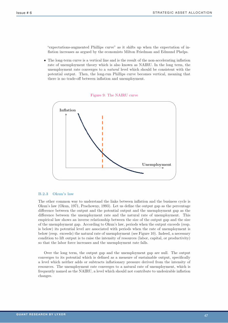
Q u a n t R e s e a R c h b y Ly x o R 47
s t r at e g i c a s s e t a l l o c at i o nissue # 6
“expectations-augmented Phillips curve” as it shifts up when the expectation of in-flation increases as argued by the economists Milton Friedman and Edmund Phelps.
• The long-term curve is a vertical line and is the result of the non-accelerating inflationrate of unemployment theory which is also known as NAIRU. In the long term, theunemployment rate converges to a natural level which should be consistent with thepotential output. Then, the long-run Phillips curve becomes vertical, meaning thatthere is no trade-off between inflation and unemployment.
Figure 9: The NAIRU curve
Unemployment
Inflation
B.2.3 Okun’s law
The other common way to understand the links between inflation and the business cycle isOkun’s law (Okun, 1971, Prachowny, 1993). Let us define the output gap as the percentagedifference between the output and the potential output and the unemployment gap as thedifference between the unemployment rate and the natural rate of unemployment. Thisempirical law shows an inverse relationship between the size of the output gap and the sizeof the unemployment gap. According to Okun’s law, periods when the output exceeds (resp.is below) its potential level are associated with periods when the rate of unemployment isbelow (resp. exceeds) the natural rate of unemployment (see Figure 10). Indeed, a necessarycondition to lift output is to raise the intensity of resources (labor, capital, or productivity)so that the labor force increases and the unemployment rate falls.
Over the long term, the output gap and the unemployment gap are null. The outputconverges to its potential which is defined as a measure of sustainable output, specificallya level which neither adds or subtracts inflationary pressure derived from the intensity ofresources. The unemployment rate converges to a natural rate of unemployment, which isfrequently named as the NAIRU, a level which should not contribute to undesirable inflationchanges.
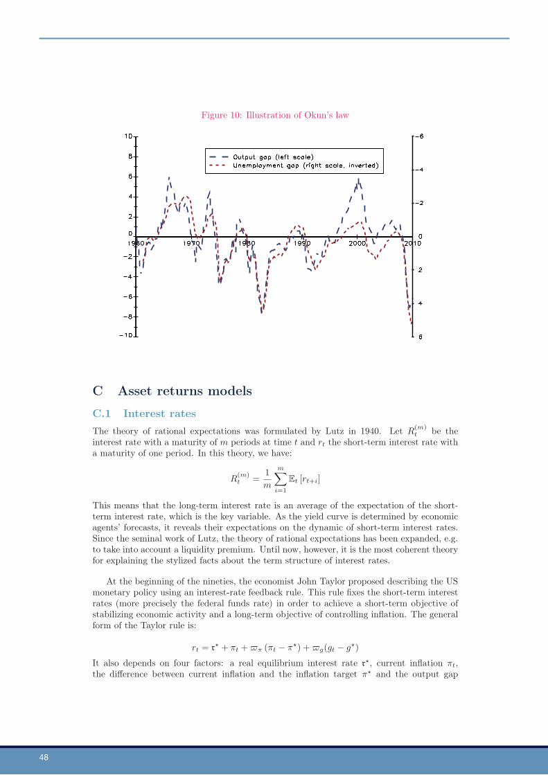
48
Figure 10: Illustration of Okun’s law
C Asset returns models
C.1 Interest ratesThe theory of rational expectations was formulated by Lutz in 1940. Let R
(m)t be the
interest rate with a maturity of m periods at time t and rt the short-term interest rate witha maturity of one period. In this theory, we have:
R(m)t =
1m
m
i=1
Et [rt+i]
This means that the long-term interest rate is an average of the expectation of the short-term interest rate, which is the key variable. As the yield curve is determined by economicagents’ forecasts, it reveals their expectations on the dynamic of short-term interest rates.Since the seminal work of Lutz, the theory of rational expectations has been expanded, e.g.to take into account a liquidity premium. Until now, however, it is the most coherent theoryfor explaining the stylized facts about the term structure of interest rates.
At the beginning of the nineties, the economist John Taylor proposed describing the USmonetary policy using an interest-rate feedback rule. This rule fixes the short-term interestrates (more precisely the federal funds rate) in order to achieve a short-term objective ofstabilizing economic activity and a long-term objective of controlling inflation. The generalform of the Taylor rule is:
rt = r + πt +π (πt − π) +g(gt − g)
It also depends on four factors: a real equilibrium interest rate r, current inflation πt,the difference between current inflation and the inflation target π and the output gap
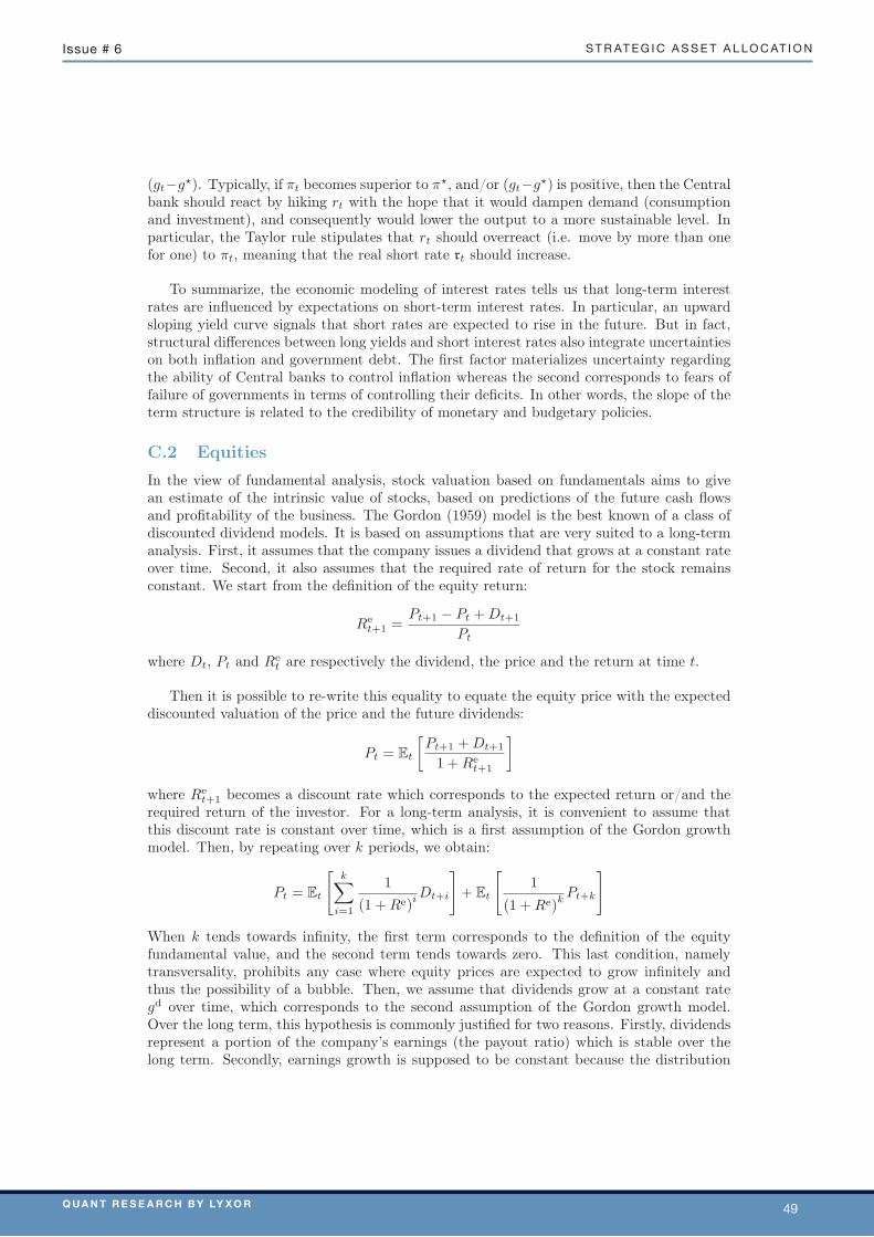
Q u a n t R e s e a R c h b y Ly x o R 49
s t r at e g i c a s s e t a l l o c at i o nissue # 6
(gt−g). Typically, if πt becomes superior to π, and/or (gt−g) is positive, then the Centralbank should react by hiking rt with the hope that it would dampen demand (consumptionand investment), and consequently would lower the output to a more sustainable level. Inparticular, the Taylor rule stipulates that rt should overreact (i.e. move by more than onefor one) to πt, meaning that the real short rate rt should increase.
To summarize, the economic modeling of interest rates tells us that long-term interestrates are influenced by expectations on short-term interest rates. In particular, an upwardsloping yield curve signals that short rates are expected to rise in the future. But in fact,structural differences between long yields and short interest rates also integrate uncertaintieson both inflation and government debt. The first factor materializes uncertainty regardingthe ability of Central banks to control inflation whereas the second corresponds to fears offailure of governments in terms of controlling their deficits. In other words, the slope of theterm structure is related to the credibility of monetary and budgetary policies.
C.2 EquitiesIn the view of fundamental analysis, stock valuation based on fundamentals aims to givean estimate of the intrinsic value of stocks, based on predictions of the future cash flowsand profitability of the business. The Gordon (1959) model is the best known of a class ofdiscounted dividend models. It is based on assumptions that are very suited to a long-termanalysis. First, it assumes that the company issues a dividend that grows at a constant rateover time. Second, it also assumes that the required rate of return for the stock remainsconstant. We start from the definition of the equity return:
Ret+1 =
Pt+1 − Pt +Dt+1
Pt
where Dt, Pt and Ret are respectively the dividend, the price and the return at time t.
Then it is possible to re-write this equality to equate the equity price with the expecteddiscounted valuation of the price and the future dividends:
Pt = Et
Pt+1 +Dt+1
1 +Ret+1
where Ret+1 becomes a discount rate which corresponds to the expected return or/and the
required return of the investor. For a long-term analysis, it is convenient to assume thatthis discount rate is constant over time, which is a first assumption of the Gordon growthmodel. Then, by repeating over k periods, we obtain:
Pt = Et
k
i=1
1
(1 +Re)iDt+i
+ Et
1
(1 +Re)kPt+k
When k tends towards infinity, the first term corresponds to the definition of the equityfundamental value, and the second term tends towards zero. This last condition, namelytransversality, prohibits any case where equity prices are expected to grow infinitely andthus the possibility of a bubble. Then, we assume that dividends grow at a constant rategd over time, which corresponds to the second assumption of the Gordon growth model.Over the long term, this hypothesis is commonly justified for two reasons. Firstly, dividendsrepresent a portion of the company’s earnings (the payout ratio) which is stable over thelong term. Secondly, earnings growth is supposed to be constant because the distribution
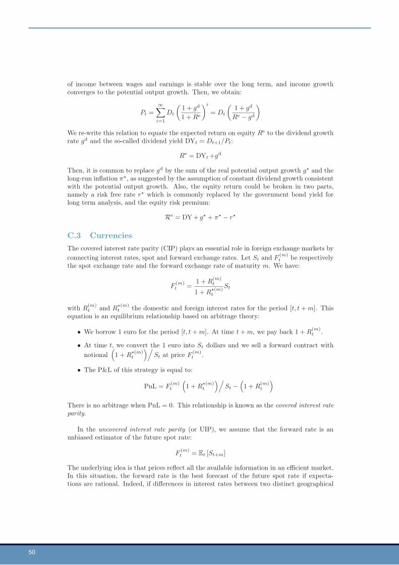
50
of income between wages and earnings is stable over the long term, and income growthconverges to the potential output growth. Then, we obtain:
Pt =∞
i=1
Dt
1 + gd
1 +Re
i
= Dt
1 + gd
Re − gd
We re-write this relation to equate the expected return on equity Re to the dividend growthrate gd and the so-called dividend yield DYt = Dt+1/Pt:
Re = DYt +gd
Then, it is common to replace gd by the sum of the real potential output growth g and thelong-run inflation π, as suggested by the assumption of constant dividend growth consistentwith the potential output growth. Also, the equity return could be broken in two parts,namely a risk free rate r which is commonly replaced by the government bond yield forlong term analysis, and the equity risk premium:
Re = DY+ g + π − r
C.3 CurrenciesThe covered interest rate parity (CIP) plays an essential role in foreign exchange markets byconnecting interest rates, spot and forward exchange rates. Let St and F
(m)t be respectively
the spot exchange rate and the forward exchange rate of maturity m. We have:
F(m)t =
1 +R(m)t
1 +R(m)t
St
with R(m)t and R
(m)t the domestic and foreign interest rates for the period [t, t+m]. This
equation is an equilibrium relationship based on arbitrage theory:
• We borrow 1 euro for the period [t, t+m]. At time t+m, we pay back 1 +R(m)t .
• At time t, we convert the 1 euro into St dollars and we sell a forward contract withnotional
1 +R
(m)t
St at price F
(m)t .
• The P&L of this strategy is equal to:
PnL = F(m)t
1 +R
(m)t
St −
1 +R
(m)t
There is no arbitrage when PnL = 0. This relationship is known as the covered interest rateparity.
In the uncovered interest rate parity (or UIP), we assume that the forward rate is anunbiased estimator of the future spot rate:
F(m)t = Et [St+m]
The underlying idea is that prices reflect all the available information in an efficient market.In this situation, the forward rate is the best forecast of the future spot rate if expecta-tions are rational. Indeed, if differences in interest rates between two distinct geographical
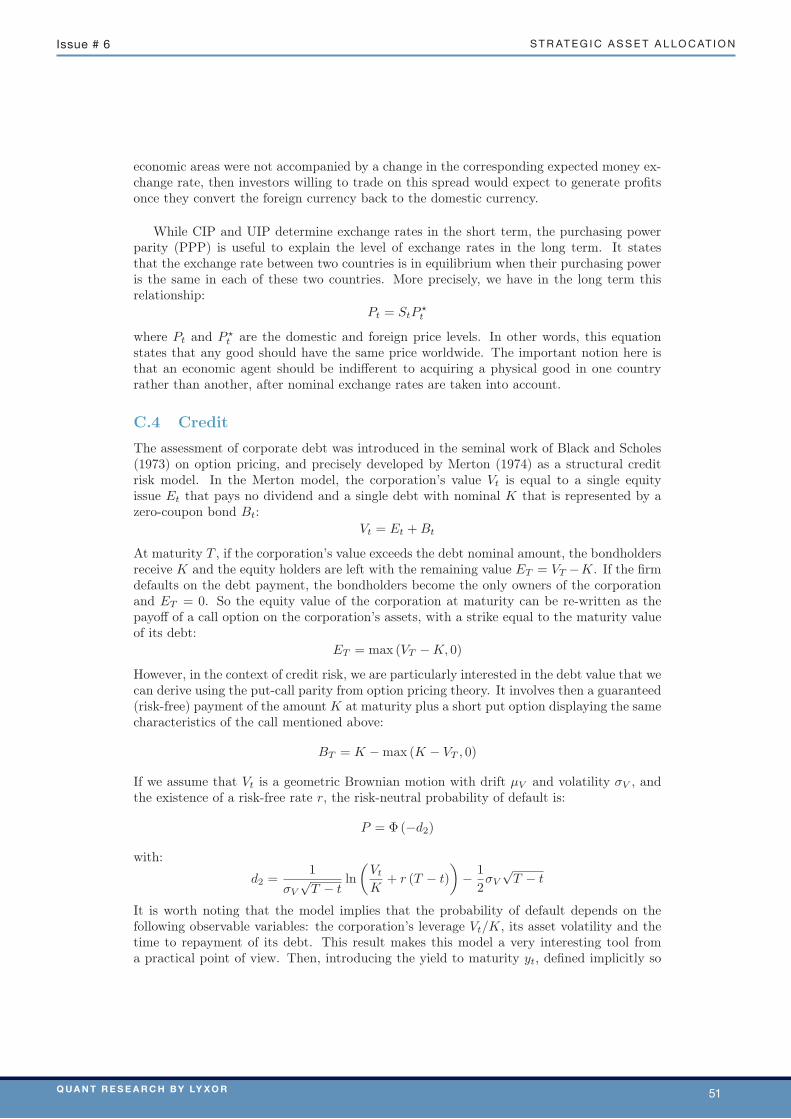
Q u a n t R e s e a R c h b y Ly x o R 51
s t r at e g i c a s s e t a l l o c at i o nissue # 6
economic areas were not accompanied by a change in the corresponding expected money ex-change rate, then investors willing to trade on this spread would expect to generate profitsonce they convert the foreign currency back to the domestic currency.
While CIP and UIP determine exchange rates in the short term, the purchasing powerparity (PPP) is useful to explain the level of exchange rates in the long term. It statesthat the exchange rate between two countries is in equilibrium when their purchasing poweris the same in each of these two countries. More precisely, we have in the long term thisrelationship:
Pt = StPt
where Pt and P t are the domestic and foreign price levels. In other words, this equation
states that any good should have the same price worldwide. The important notion here isthat an economic agent should be indifferent to acquiring a physical good in one countryrather than another, after nominal exchange rates are taken into account.
C.4 Credit
The assessment of corporate debt was introduced in the seminal work of Black and Scholes(1973) on option pricing, and precisely developed by Merton (1974) as a structural creditrisk model. In the Merton model, the corporation’s value Vt is equal to a single equityissue Et that pays no dividend and a single debt with nominal K that is represented by azero-coupon bond Bt:
Vt = Et +Bt
At maturity T , if the corporation’s value exceeds the debt nominal amount, the bondholdersreceive K and the equity holders are left with the remaining value ET = VT −K. If the firmdefaults on the debt payment, the bondholders become the only owners of the corporationand ET = 0. So the equity value of the corporation at maturity can be re-written as thepayoff of a call option on the corporation’s assets, with a strike equal to the maturity valueof its debt:
ET = max (VT −K, 0)
However, in the context of credit risk, we are particularly interested in the debt value that wecan derive using the put-call parity from option pricing theory. It involves then a guaranteed(risk-free) payment of the amount K at maturity plus a short put option displaying the samecharacteristics of the call mentioned above:
BT = K −max (K − VT , 0)
If we assume that Vt is a geometric Brownian motion with drift µV and volatility σV , andthe existence of a risk-free rate r, the risk-neutral probability of default is:
P = Φ(−d2)
with:
d2 =1
σV
√T − t
lnVt
K+ r (T − t)
− 1
2σV
√T − t
It is worth noting that the model implies that the probability of default depends on thefollowing observable variables: the corporation’s leverage Vt/K, its asset volatility and thetime to repayment of its debt. This result makes this model a very interesting tool froma practical point of view. Then, introducing the yield to maturity yt, defined implicitly so

52
that Bt = Ke−yt(T−t), it is possible to obtain the expression for the so-called credit spreadas an increasing function f of the default probability PD:
st = yt − r = f (PD)
The pricing of default probabilities implying credit spreads is consistent with a risk-neutralworld. In practical terms, in a risk averse world, the corporate bond yield is actuallycomprised of a government bond yield (assuming that governments never default), plus acredit risk premium that is positively correlated to the firm’s default probability but thatdepends also on the uncertainty on the default probability (materialized through the firm’sasset volatility).
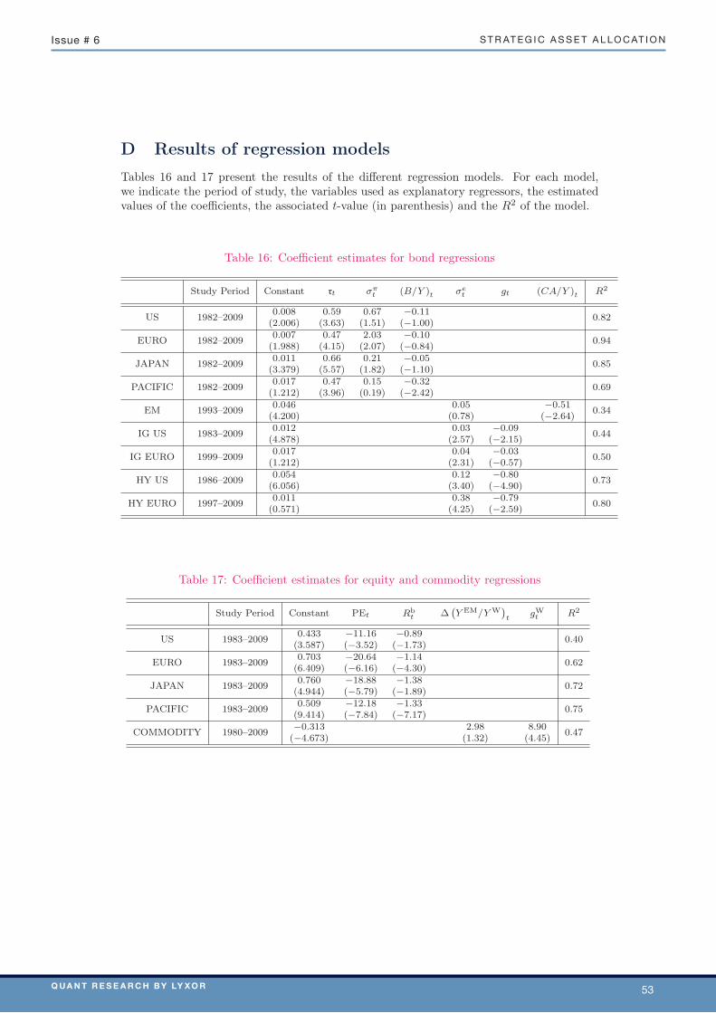
Q u a n t R e s e a R c h b y Ly x o R 53
s t r at e g i c a s s e t a l l o c at i o nissue # 6
D Results of regression modelsTables 16 and 17 present the results of the different regression models. For each model,we indicate the period of study, the variables used as explanatory regressors, the estimatedvalues of the coefficients, the associated t-value (in parenthesis) and the R2 of the model.
Table 16: Coefficient estimates for bond regressions
Study Period Constant rt σπt (B/Y )t σet gt (CA/Y )t R2
US 1982–2009 0.008 0.59 0.67 −0.110.82
(2.006) (3.63) (1.51) (−1.00)EURO 1982–2009 0.007 0.47 2.03 −0.10
0.94(1.988) (4.15) (2.07) (−0.84)
JAPAN 1982–2009 0.011 0.66 0.21 −0.050.85
(3.379) (5.57) (1.82) (−1.10)PACIFIC 1982–2009 0.017 0.47 0.15 −0.32
0.69(1.212) (3.96) (0.19) (−2.42)
EM 1993–2009 0.046 0.05 −0.510.34
(4.200) (0.78) (−2.64)IG US 1983–2009 0.012 0.03 −0.09
0.44(4.878) (2.57) (−2.15)
IG EURO 1999–2009 0.017 0.04 −0.030.50
(1.212) (2.31) (−0.57)HY US 1986–2009 0.054 0.12 −0.80
0.73(6.056) (3.40) (−4.90)
HY EURO 1997–2009 0.011 0.38 −0.790.80
(0.571) (4.25) (−2.59)
Table 17: Coefficient estimates for equity and commodity regressions
Study Period Constant PEt Rbt ∆
`Y EM/Y W
´t
gWt R2
US 1983–2009 0.433 −11.16 −0.890.40
(3.587) (−3.52) (−1.73)EURO 1983–2009 0.703 −20.64 −1.14
0.62(6.409) (−6.16) (−4.30)
JAPAN 1983–2009 0.760 −18.88 −1.380.72
(4.944) (−5.79) (−1.89)PACIFIC 1983–2009 0.509 −12.18 −1.33
0.75(9.414) (−7.84) (−7.17)
COMMODITY 1980–2009 −0.313 2.98 8.900.47
(−4.673) (1.32) (4.45)
54
References
[1] Ambachtsheer K.P. (1987), Pension Fund Asset Allocation: In Defense of a 60/40Equity/Debt Asset Mix, Financial Analysts Journal, 43(5), pp. 14-24.
[2] Amin G.S. and Kat H.M. (2003), Stocks, Bonds, and Hedge Funds, Journal of PortfolioManagement, 29(4), pp. 113-120.
[3] Baker D., DeLong B. and Krugman P. (2005), Asset returns and Economic Growth,Brookings Papers on Economic Activity, 1, pp. 289-315.
[4] Bansal R. and Yaron A. (2004), Risks for the Long Run: A Potential Resolution ofAsset Pricing Puzzles, Journal of Finance, 59(4), pp. 1481-1509.
[5] Bansal R., Kiku D. and Yaron A. (2010), Long Run Risks, the Macroeconomy, andAsset Prices, American Economic Review, 100(2), pp. 542-546.
[6] Ball L. and Mankiw N.G. (2002), The NAIRU in Theory and Practice, Journal ofEconomic Perspectives, 16(4), pp. 115-136.
[7] Barberis N. (2000), Investing for the Long Run when Returns are Predictable, Journalof Finance, 55(1), pp. 225-264.
[8] Barro R.J. and Gordon D.B. (1983), A Positive Theory of Monetary Policy in aNatural Rate Model, Journal of Political Economy, 91(4), pp. 589-610.
[9] Barro R.J., Mankiw N.G. and Sala-I-Martin X. (1995), Capital Mobility in Neo-classical Models of Growth, American Economic Review, 85(1), pp. 103-115.
[10] Barro R.J. and Sala-I-Martin X. (1995), Economic Growth, McGraw-Hill.
[11] Bekkers N., Doeswijk R.Q. and Lam T.W. (2009), Strategic Asset Alloca-tion: Determining the Optimal Portfolio with Ten Asset Classes Working Paper,ssrn.com/abstract=1368689.
[12] Bernanke B.S., Laubach T., Mishkin F.S. and Posen A.S. (1999), Inflation Tar-geting: Lessons from the International Experience, Princeton University Press.
[13] Beveridge S. and Nelson C.R. (1981), A New Approach to the Decomposition ofEconomic Time Series into Permanent and Transitory Components with ParticularAttention to Measurement of the Business Cycle, Journal of Monetary Economics,7(2), pp. 151-174.
[14] Black F. and Litterman R.B., Global Portfolio Optimization, Financial AnalystsJournal, 48(5), 1992, p. 28-43.
[15] Blanchard O. and Katz L.F. (1997), What We Know and Do Not Know About theNatural Rate of Unemployment, Journal of Economic Perspectives, 11(1), pp. 57-72.
[16] Blake D., Lehmann B.N. and Timmermann A. (1999), Asset Allocation Dynamicsand Pension Fund Performance, Journal of Business, 72(4), pp. 429-461.
[17] Bruder B., Jamet G. and Lasserre G. (2010), Beyond Liability-Driven Investment:New Perspectives on Defined Benefit Pension Fund Management, Lyxor White PaperSeries, 2, www.lyxor.com.

Q u a n t R e s e a R c h b y Ly x o R 55
s t r at e g i c a s s e t a l l o c at i o nissue # 6
[18] Bruno M. and Easterly W. (1998), Inflation Crises and Long-Run Growth, Journalof Monetary Economics, 41(1), pp. 3-26.
[19] Cahuc P. and Zylberberg A. (2004), Labor Economics, MIT Press.
[20] Campbell J.Y. (1999), Asset Prices, Consumption and the Business Cycle, in J. Taylorand M. Woodford (eds.), Handbook of Macroeconomics, 1(3), pp. 1231-1303, Elsevier.
[21] Campbell J.Y. and Ammer J. (1993), What Moves the Stock and Bond Markets? AVariance Decomposition for Long-Term Asset Returns, Journal of Finance, 48(1), pp.3-37.
[22] Campbell J.Y. and Cochrane J.H. (1999), By Force of Habit: A Consumption-BasedExplanation of Aggregate Stock Market Behavior, Journal of Political Economy, 107(2),pp. 205-251.
[23] Campbell J.Y. and Shiller R.J. (1988), The Dividend-Price Ratio and Expectationsof Future Dividends and Discount Factors, Review of Financial Studies, 1(3), pp. 195-228.
[24] Campbell J.Y. and Shiller R.J. (1988), Stock Prices, Earnings, and Expected Divi-dends, Journal of Finance, 43(3), pp. 661-676.
[25] Campbell J.Y. and Shiller R.J. (1991), Yield Spreads and Interest Rate Movements:A Bird’s Eye View, Review of Economic Studies, 58(3), pp. 495-514.
[26] Campbell J.Y. and Shiller R.J. (1998), Valuation Ratios and the Long-Run StockMarket Outlook, Journal of Portfolio Management, 24(2), pp. 11-26.
[27] Campbell J.Y. and Viceira L. (2002), Strategic Asset Allocation: Portfolio Choicefor Long Term Investors, Oxford University Press.
[28] Clarida R.H. and Friedman B.M. (1983), Why Have Short-Term Interest Rates BeenSo High?, Brookings Papers on Economic Activity, 2, pp. 553-585.
[29] Cochrane J.H. (1991), Production-Based Asset Pricing and the Link Between StockReturns and Economic Fluctuations, Journal of Finance, 46(1), pp. 209-237.
[30] Cochrane J.H. (2001), Asset Pricing, Princeton University Press.
[31] Cochrane J.H. and Piazzesi M. (2005), Bond Risk Premia, American EconomicReview, 95(1), pp. 138-160.
[32] Darolles S., Eychenne K. and Martinetti S. (2010), Time-varying Risk Premiumsand Business Cycle: A Survey, Lyxor White Paper Series, 4, www.lyxor.com.
[33] Deaton A. and Laroque G. (1992), On the Behaviour of Commodity Prices, Reviewof Economic Studies, 59(1), pp. 1-23.
[34] Diebold F.X. and Yilmaz K. (2010), Macroeconomic Volatility and Stock MarketVolatility, Worldwide, in Russell J. and Watson M. (eds.), Volatility and Time SeriesEconometrics: Essays in Honor of Robert F. Engle, Oxford University Press, pp. 97-116.
[35] Dimson E., Marsh P. and Staunton M. (2010), Global Investment Returns Source-book 2010, Credit Suisse.
56
[36] Erb C.B. and Harvey C.R. (2006), The Tactical and Strategic Value of CommodityFutures, Financial Analysts Journal, 62(2), pp. 69-97.
[37] Engle E.F. and Granger C.W.J. (1987), Co-Integration and Error Correction: Rep-resentation, Estimation, and Testing , Econometrica, 55(2), pp. 251-276.
[38] Fama E.F. and Bliss R. (1987), The Information in Long-Maturity Forward Rates,American Economic Review, 77(4), pp. 680-692.
[39] Fama E. and French K.R. (2002), The Equity Premium, Journal of Finance, 57(2),pp. 637-659.
[40] Favero C., Gozluklu A. and Tamoni A. (2009), Demographic Trends, the Dividend-Price Ratio and the Predictability of Long-Run Stock Market Returns, forthcoming inJournal of Financial and Quantitative Analysis.
[41] Fisher I. (1896), Appreciation and Interest, American Economic Association.
[42] Francis N. and Ramey V.A. (2005), Is the Technology-driven Real Business CycleHypothesis Dead? Shocks and Aggregate Fluctuations Revisited, Journal of MonetaryEconomics, 52(8), pp. 1379-1399.
[43] Friedman B.M. (2003), The Use and Meaning of Words in Central Banking: InflationTargeting, Credibility and Transparency, in Mizen P. (ed.), Central Banking, MonetaryTheory and Practice, Edward Elgar.
[44] Frenkel J.A. and Levich R.M. (1975), Covered Interest Arbitrage: Unexploited Prof-its?, Journal of Political Economy, 83(2), pp. 325-338.
[45] Fugazza C., Guidolin M. and Nicodano G. (2007), Investing for the Long-Run inEuropean Real Estate, Journal of Real Estate Finance and Economics, 34(1), pp. 35-80.
[46] Gordon M.J. (1959), Dividends, Earnings, and Stock Prices, Review of Economicsand Statistics, 41(2), pp 99-105.
[47] Gordon R.J. (1997), The Time-Varying NAIRU and its Implications for EconomicPolicy, Journal of Economic Perspectives, 11(1), pp 11-32.
[48] Hodrick R. and Prescott E. (1997), Post-war US Business Cycles: An EmpiricalInvestigation, Journal of Money, Credit and Banking, 29(1), pp 1-16.
[49] Ibbotson Associates (2009), Market Results for Stocks, Bonds, Bills, and Inflation 1926-2008, Ibbotson SBBI 2009 Classic Yearbook, Morningstar.
[50] Ilmanen A. (2003), Stock-Bond Correlations, Journal of Fixed Income, 13(2), pp. 55-66.
[51] Jones E.P., Mason S.P. and Rosenfeld E. (1984), Contingent Claims Analysis ofCorporate Capital Structure: An Empirical Investigation, Journal of Finance, 39(3),pp. 611-625.
[52] Kaldor N. (1939), Speculation and Economic Stability, Review of Economic Studies,7(1), pp. 1-27.
[53] Keynes J.M. (1923), Some Aspects of Commodity Markets, Manchester Guardian.
Q u a n t R e s e a R c h b y Ly x o R 57
s t r at e g i c a s s e t a l l o c at i o nissue # 6
[54] King R.G. and Rebelo S.T. (1999), Resuscitating Real Business Cycles, in J.B. Taylorand M. Woodford (eds.), Handbook of Macroeconomics, 1(2), pp. 927-1007, Elsevier.
[55] Kydland F.E. and Prescott E.C. (1991), Hours and Employment Variation in Busi-ness Cycle Theory, Economic Theory, 1(1), pp. 63-81.
[56] Li L. (2002), Macroeconomic Factors and the Correlation of Stock and Bond Returns,Yale ICF Working Paper, 02-46, ssrn.com/abstract=363641.
[57] Lucas R. (1978), Asset Prices in an Exchange Economy, Econometrica, 46(6), pp.1429-1445.
[58] Lutz F.A. (1940), The Structure of Interest Rates, Quarterly Journal of Economics,55, pp. 36-63.
[59] Marcussen, M. (2006), Long Term Outlook, Strategy and Economic Research, SociétéGénérale Asset Management.
[60] Merton, R.C. (1971), Optimum Consumption and Portfolio Rules in a Continuous-Time Model, Journal of Economic Theory, 3(4), pp. 373-413.
[61] Merton R.C. (1973), An Intertemporal Capital Asset Pricing Model, Econometrica,41(5), pp. 867-887.
[62] Merton R.C. (1974), On the Pricing of Corporate Debt: The Risk Structure of InterestRates, Journal of Finance, 29, pp. 449-470.
[63] Michaud R.O. (1989), The Markowitz Optimization Enigma: Is “Optimized” Opti-mal?, Financial Analysts Journal, 45(1), pp. 31-42.
[64] Norman E.J., Sirmans S.G. and Benjamin J.D. (1995), The Historical Environmentof Real Estate Returns, Journal of Real Estate Portfolio Management, 1(1), pp. 1-24.
[65] Okun A.M. (1971), The Mirage of Steady Inflation, Brookings Papers on EconomicActivity, 2, pp. 485-498.
[66] Phelps E. (1961), The Golden Rule of Accumulation: A Fable for Growthmen, Amer-ican Economic Review, 51(4), pp. 638-643.
[67] Phalippou L. (2007), Investing in Private Equity Funds: A Survey, CFA InstituteLiterature Survey Series.
[68] Phillips A.W. (1958), The Relation between Unemployment and the Rate of Changeof Money Wage Rates in the United Kingdom, 1861–1957, Economica, 25(100), pp.283-299.
[69] Prachowny M.F.J. (1993), Okun’s Law: Theoretical Foundations and Revised Esti-mates, Review of Economics and Statistics, 75(2), pp. 331-336.
[70] Roncalli T. (2011), Understanding the Impact of Weights Constraints in PortfolioTheory, Working Paper, ssrn.com/abstract=1761625.
[71] Roncalli T. and Teiletche J. (2008), An Alternative Approach to Alternative Beta,Journal of Financial Transformation, 24, pp. 43-52.
[72] Roxburgh C., Lund S., Lippert M., White O.L. and Zhao Y. (2009), The NewPower Brokers: How Oil, Asia, Hedge Funds, and Private Equity are Shaping GlobalCapital Markets, McKinsey Global Institute.
58
[73] Rudebusch G.D. and Wu T. (2008), A Macro-Finance Model of the Term Structure,Monetary Policy and the Economy, Economic Journal, 118(530), pp. 906-926.
[74] Samuelson P. and Solow R. (1960), Analytical Aspects of Anti-Inflation Policy,American Economic Review, 50(2), pp. 177-194.
[75] Shiller R.J (1981), Do Prices Move Too Much to be Justified by Subsequent Changesin Dividends?, American Economic Review, 71(3), pp. 421-436.
[76] Smets F. and Wouters R. (2005), Comparing Shocks and Frictions in US and EuroArea Business Cycles: A Bayesian DSGE Approach, Journal of Applied Econometrics,20(2), pp. 161-183.
[77] Solow R. (1956), A Contribution to the Theory of Economic Growth, Quarterly Jour-nal of Economics, 70(1), pp. 65-94.
[78] Sørensen B.E., Wu Y-T., Yosha O. and Zhu Y. (2007), Home Bias and InternationalRisk Sharing: Twin Puzzles Separated at Birth, Journal of International Money andFinance, 26(4), pp. 587-605.
[79] Sutcliffe C. (2005), The Cult of the Equity for Pension Funds: Should it Get theBoot?, Journal of Pension Economics and Finance, 4(1), pp. 57-85.
[80] Tang S.H.K. (2002), The Link Between Growth Volatility and Technical Progress:Cross-Country Evidence, Economics Letters, 77(3), pp. 335-341.
[81] Taylor J.B. (1993), Discretion Versus Policy Rules in Practice, Carnegie-RochesterConference Series on Public Policy, 39, pp. 195-214.
[82] USDA (2010), Agricultural Projections to 2019, Long-term Projections Report, OCE-2010-1.
[83] Wilshire Consulting (2009), Report on State Retirement Systems: Funding Levels andAsset Allocation.
[84] Woodford M. (2003), Interest and Prices: Foundations of a Theory of MonetaryPolicy, Princeton University Press.

Q u a n t R e s e a R c h b y Ly x o R 59
s t r at e g i c a s s e t a l l o c at i o nissue # 6
Lyxor White Paper Series
List of Issues
• Issue #1 – Risk-Based Indexation.
Paul Demey, Sébastien Maillard and Thierry Roncalli, March 2010.
• Issue #2 – Beyond Liability-Driven Investment: New Perspectives onDefined Benefit Pension Fund Management.
Benjamin Bruder, Guillaume Jamet and Guillaume Lasserre, March 2010.
• Issue #3 – Mutual Fund Ratings and Performance Persistence.
Pierre Hereil, Philippe Mitaine, Nicolas Moussavi and Thierry Roncalli, June 2010.
• Issue #4 – Time Varying Risk Premiums & Business Cycles: A Survey.
Serge Darolles, Karl Eychenne and Stéphane Martinetti, September 2010.
• Issue #5 – Portfolio Allocation of Hedge Funds.
Benjamin Bruder, Serge Darolles, Abdul Koudiraty and Thierry Roncalli, January2010.

60

Q u a n t R e s e a R c h b y Ly x o R 61
s t r at e g i c a s s e t a l l o c at i o nissue # 6
Disclaimer
Each of this material and its content is confidential and may not be reproduced or providedto others without the express written permission of Lyxor Asset Management (“Lyxor AM”).This material has been prepared solely for informational purposes only and it is not intendedto be and should not be considered as an offer, or a solicitation of an offer, or an invitationor a personal recommendation to buy or sell participating shares in any Lyxor Fund, orany security or financial instrument, or to participate in any investment strategy, directlyor indirectly.
It is intended for use only by those recipients to whom it is made directly available by LyxorAM. Lyxor AM will not treat recipients of this material as its clients by virtue of theirreceiving this material.
This material reflects the views and opinions of the individual authors at this date and inno way the official position or advices of any kind of these authors or of Lyxor AM and thusdoes not engage the responsibility of Lyxor AM nor of any of its officers or employees. Allperformance information set forth herein is based on historical data and, in some cases, hy-pothetical data, and may reflect certain assumptions with respect to fees, expenses, taxes,capital charges, allocations and other factors that affect the computation of the returns.Past performance is not necessarily a guide to future performance. While the information(including any historical or hypothetical returns) in this material has been obtained fromexternal sources deemed reliable, neither Société Générale (“SG”), Lyxor AM, nor their af-filiates, officers employees guarantee its accuracy, timeliness or completeness. Any opinionsexpressed herein are statements of our judgment on this date and are subject to change with-out notice. SG, Lyxor AM and their affiliates assume no fiduciary responsibility or liabilityfor any consequences, financial or otherwise, arising from, an investment in any security orfinancial instrument described herein or in any other security, or from the implementationof any investment strategy.
Lyxor AM and its affiliates may from time to time deal in, profit from the trading of, hold,have positions in, or act as market makers, advisers, brokers or otherwise in relation to thesecurities and financial instruments described herein.
Service marks appearing herein are the exclusive property of SG and its affiliates, as thecase may be.
This material is communicated by Lyxor Asset Management, which is authorized and reg-ulated in France by the “Autorité des Marchés Financiers” (French Financial Markets Au-thority).
c 2010 LYXOR ASSET MANAGEMENT ALL RIGHTS RESERVED

Lyxor Asset ManagementTour Société Générale – 17, cours Valmy
92987 Paris – La Défense Cedex – Francewww.lyxor.com
Publishing Directors
alain Dubois, Chairman of the Board
Laurent seyer, Chief Executive Officer
nicolas Gaussel, PhD, Head of Quantitative Asset Management
eDitorial boarD
serge Darolles, PhD, Managing Editor
thierry Roncalli, PhD, Associate Editor
Guillaume Jamet, PhD, Associate Editor
the lyxor White Paper series is a quarterly publication providing our clients access to intellectual capital, risk analytics and quantitative research developed within lyxor asset Management. the series covers in depth studies of investment strategies, asset allocation methodologies and risk management techniques. We hope you will find the Lyxor White Paper Series stimulating and interesting.
Réf
. 71
1267
– S
tudi
o S
ocié
té G
énér
ale
+33
(0)1
42
14 2
7 05
– 0
3/20
11