Embed Size (px)
Citation preview
Helmholtz Wave Equation TE, TM, and TEM Modes – Rect Rectangular Waveguide TE, TM, and TEM Modes – Cyl Cylindrical Waveguide
Waveguides
S. R. [email protected]
Department of Electrical & Electronics EngineeringBITS Pilani, Hyderbad Campus
May 7, 2015
Vector Calculus EE208, School of Electronics Engineering, VIT
Helmholtz Wave Equation TE, TM, and TEM Modes – Rect Rectangular Waveguide TE, TM, and TEM Modes – Cyl Cylindrical Waveguide
Outline
1 Helmholtz Wave Equation
2 TE, TM, and TEM Modes – Rect
3 Rectangular Waveguide
4 TE, TM, and TEM Modes – Cyl
5 Cylindrical Waveguide
Vector Calculus EE208, School of Electronics Engineering, VIT
Helmholtz Wave Equation TE, TM, and TEM Modes – Rect Rectangular Waveguide TE, TM, and TEM Modes – Cyl Cylindrical Waveguide
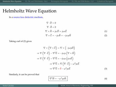
Helmholtz Wave EquationIn a source-less dielectric medium,
∇ · ~D = 0
∇ ·~B = 0
∇× ~H = jω~D = jωε~E (1)
∇×~E = −jω~B = −jωµ~H (2)
Taking curl of (2) gives
∇×(∇×~E
)= ∇×
(−jωµ~H
)⇒ ∇
(∇ ·~E
)−∇2~E = −jωµ
(∇× ~H
)⇒ ∇
(∇ ·~E
)−∇2~E = −jωµ
(jωε~E
)⇒ ∇2~E = ∇
(∇ ·~E
)−ω2µε~E
⇒ ∇2~E =~0−ω2µε~E (3)
Similarly, it can be proved that
∇2~H = −ω2µε~H. (4)
Vector Calculus EE208, School of Electronics Engineering, VIT
Helmholtz Wave Equation TE, TM, and TEM Modes – Rect Rectangular Waveguide TE, TM, and TEM Modes – Cyl Cylindrical Waveguide
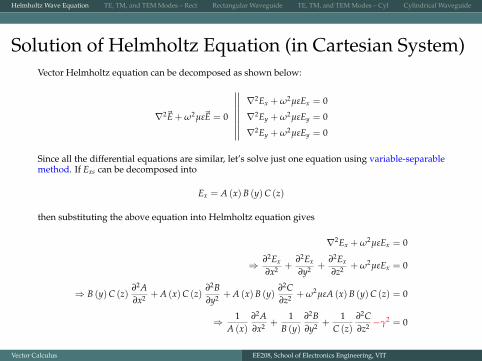
Solution of Helmholtz Equation (in Cartesian System)Vector Helmholtz equation can be decomposed as shown below:
∇2Ex + ω2µεEx = 0
∇2~E + ω2µε~E = 0 ∇2Ey + ω2µεEy = 0
∇2Ey + ω2µεEy = 0
Since all the differential equations are similar, let’s solve just one equation using variable-separablemethod. If Exs can be decomposed into
Ex = A (x)B (y)C (z)
then substituting the above equation into Helmholtz equation gives
∇2Ex + ω2µεEx = 0
⇒ ∂2Ex
∂x2 +∂2Ex
∂y2 +∂2Ex
∂z2 + ω2µεEx = 0
⇒ B (y)C (z)∂2A∂x2 + A (x)C (z)
∂2B∂y2 + A (x)B (y)
∂2C∂z2 + ω2µεA (x)B (y)C (z) = 0
⇒ 1A (x)
∂2A∂x2 +
1B (y)
∂2B∂y2 +
1C (z)
∂2C∂z2 −γ2 = 0
Vector Calculus EE208, School of Electronics Engineering, VIT
Helmholtz Wave Equation TE, TM, and TEM Modes – Rect Rectangular Waveguide TE, TM, and TEM Modes – Cyl Cylindrical Waveguide
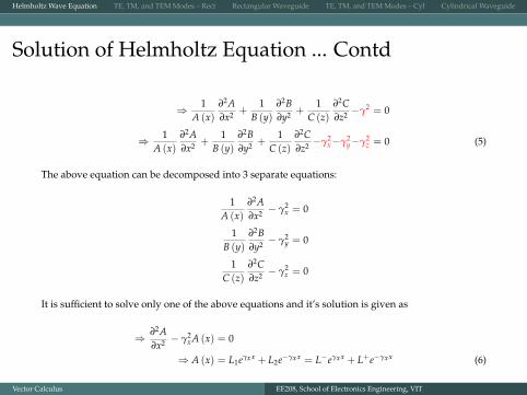
Solution of Helmholtz Equation ... Contd
⇒ 1A (x)
∂2A∂x2 +
1B (y)
∂2B∂y2 +
1C (z)
∂2C∂z2 −γ2 = 0
⇒ 1A (x)
∂2A∂x2 +
1B (y)
∂2B∂y2 +
1C (z)
∂2C∂z2 −γ2
x−γ2y−γ2
z = 0 (5)
The above equation can be decomposed into 3 separate equations:
1A (x)
∂2A∂x2 − γ2
x = 0
1B (y)
∂2B∂y2 − γ2
y = 0
1C (z)
∂2C∂z2 − γ2
z = 0
It is sufficient to solve only one of the above equations and it’s solution is given as
⇒ ∂2A∂x2 − γ2
xA (x) = 0
⇒ A (x) = L1eγxx + L2e−γxx = L−eγxx + L+e−γxx (6)
Vector Calculus EE208, School of Electronics Engineering, VIT
Helmholtz Wave Equation TE, TM, and TEM Modes – Rect Rectangular Waveguide TE, TM, and TEM Modes – Cyl Cylindrical Waveguide
Solution of Helmholtz Equation ... Contd
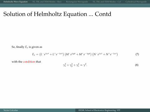
So, finally Ex is given as
Ex =(L−eγxx + L+e−γxx) (M−eγyy + M+e−γyy) (N−eγzz + N+e−γzz) (7)
with the condition thatγ2
x + γ2y + γ2
z = γ2. (8)
Vector Calculus EE208, School of Electronics Engineering, VIT
Helmholtz Wave Equation TE, TM, and TEM Modes – Rect Rectangular Waveguide TE, TM, and TEM Modes – Cyl Cylindrical Waveguide
Outline
1 Helmholtz Wave Equation
2 TE, TM, and TEM Modes – Rect
3 Rectangular Waveguide
4 TE, TM, and TEM Modes – Cyl
5 Cylindrical Waveguide
Vector Calculus EE208, School of Electronics Engineering, VIT
Helmholtz Wave Equation TE, TM, and TEM Modes – Rect Rectangular Waveguide TE, TM, and TEM Modes – Cyl Cylindrical Waveguide
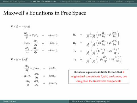
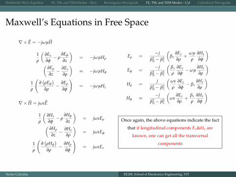
Maxwell’s Equations in Free Space
∇×~E = −jωµ~H
∂Ez
∂y+ jβzEy = −jωµHx
−jβzEx −∂Ez
∂x= −jωµHy
∂Ey
∂x− ∂Ex
∂y= −jωµHz
∇× ~H = jωε~E
∂Hz
∂y+ jβzHy = jωεEx
−jβzHx −∂Hz
∂x= jωεEy
∂Hy
∂x− ∂Hx
∂y= jωµεEz
Hx =j
β20 − β2
z
(ωε
∂Ez
∂y− βz
∂Hz
∂x
)Hy =
−jβ2
0 − β2z
(ωε
∂Ez
∂x+ βz
∂Hz
∂y
)Ex =
−jβ2
0 − β2z
(βz
∂Ez
∂x+ ωµ
∂Hz
∂y
)Ey =
jβ2
0 − β2z
(−βz
∂Ez
∂y+ ωµ
∂Hz
∂x
)
The above equations indicate the fact that if
longitudinal components Ez&Hz are known, one
can get all the transversal components
Vector Calculus EE208, School of Electronics Engineering, VIT
Helmholtz Wave Equation TE, TM, and TEM Modes – Rect Rectangular Waveguide TE, TM, and TEM Modes – Cyl Cylindrical Waveguide
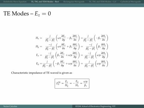
TE Modes – Ez = 0
Hx =j
β20 − β2
z
(ωε
∂Ez
∂y− βz
∂Hz
∂x
)=
jβ2
0 − β2z
(−βz
∂Hz
∂x
)Hy =
−jβ2
0 − β2z
(ωε
∂Ez
∂x+ βz
∂Hz
∂y
)=
−jβ2
0 − β2z
(βz
∂Hz
∂y
)Ex =
−jβ2
0 − β2z
(βz
∂Ez
∂x+ ωµ
∂Hz
∂y
)=
−jβ2
0 − β2z
(ωµ
∂Hz
∂y
)Ey =
jβ2
0 − β2z
(−βz
∂Ez
∂y+ ωµ
∂Hz
∂x
)=
jβ2
0 − β2z
(ωµ
∂Hz
∂x
)
Characteristic impedance of TE waved is given as
ZTE0 =
Ex
Hy= −
Ey
Hx=
ωµ
βz
Vector Calculus EE208, School of Electronics Engineering, VIT
Helmholtz Wave Equation TE, TM, and TEM Modes – Rect Rectangular Waveguide TE, TM, and TEM Modes – Cyl Cylindrical Waveguide
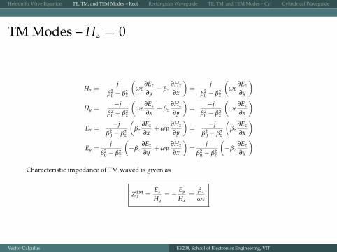
TM Modes – Hz = 0
Hx =j
β20 − β2
z
(ωε
∂Ez
∂y− βz
∂Hz
∂x
)=
jβ2
0 − β2z
(ωε
∂Ez
∂y
)Hy =
−jβ2
0 − β2z
(ωε
∂Ez
∂x+ βz
∂Hz
∂y
)=
−jβ2
0 − β2z
(ωε
∂Ez
∂x
)Ex =
−jβ2
0 − β2z
(βz
∂Ez
∂x+ ωµ
∂Hz
∂y
)=
−jβ2
0 − β2z
(βz
∂Ez
∂x
)Ey =
jβ2
0 − β2z
(−βz
∂Ez
∂y+ ωµ
∂Hz
∂x
)=
jβ2
0 − β2z
(−βz
∂Ez
∂y
)
Characteristic impedance of TM waved is given as
ZTM0 =
Ex
Hy= −
Ey
Hx=
βz
ωε
Vector Calculus EE208, School of Electronics Engineering, VIT
Helmholtz Wave Equation TE, TM, and TEM Modes – Rect Rectangular Waveguide TE, TM, and TEM Modes – Cyl Cylindrical Waveguide
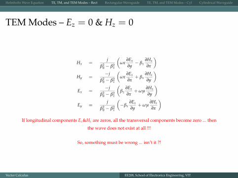
TEM Modes – Ez = 0 & Hz = 0
Hx =j
β20 − β2
z
(ωε
∂Ez
∂y− βz
∂Hz
∂x
)Hy =
−jβ2
0 − β2z
(ωε
∂Ez
∂x+ βz
∂Hz
∂y
)Ex =
−jβ2
0 − β2z
(βz
∂Ez
∂x+ ωµ
∂Hz
∂y
)Ey =
jβ2
0 − β2z
(−βz
∂Ez
∂y+ ωµ
∂Hz
∂x
)
If longitudinal components Ez&Hz are zeros, all the transversal components become zero ... then
the wave does not exist at all !!!
So, something must be wrong ... isn’t it ?!
Vector Calculus EE208, School of Electronics Engineering, VIT
Helmholtz Wave Equation TE, TM, and TEM Modes – Rect Rectangular Waveguide TE, TM, and TEM Modes – Cyl Cylindrical Waveguide
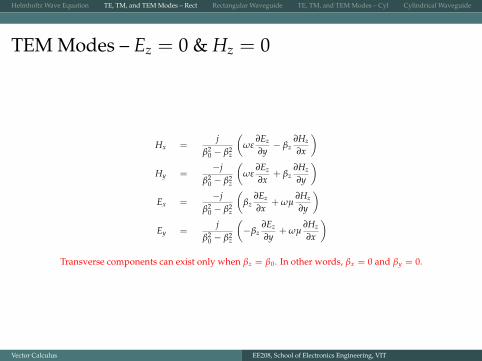
TEM Modes – Ez = 0 & Hz = 0
Hx =j
β20 − β2
z
(ωε
∂Ez
∂y− βz
∂Hz
∂x
)Hy =
−jβ2
0 − β2z
(ωε
∂Ez
∂x+ βz
∂Hz
∂y
)Ex =
−jβ2
0 − β2z
(βz
∂Ez
∂x+ ωµ
∂Hz
∂y
)Ey =
jβ2
0 − β2z
(−βz
∂Ez
∂y+ ωµ
∂Hz
∂x
)
Transverse components can exist only when βz = β0. In other words, βx = 0 and βy = 0.
Vector Calculus EE208, School of Electronics Engineering, VIT
Helmholtz Wave Equation TE, TM, and TEM Modes – Rect Rectangular Waveguide TE, TM, and TEM Modes – Cyl Cylindrical Waveguide
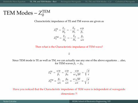
TEM Modes – ZTEM0
Characteristic impedance of TE and TM waves are given as
ZTE0 =
Ex
Hy= −
Ey
Hx=
ωµ
βz
ZTM0 =
Ex
Hy= −
Ey
Hx=
βz
ωε
Then what is the Characteristic impedance of TEM wave?
⇓
Since TEM mode is TE as well as TM, we can actually use any one of the above equations ... also,for TEM waves βz = β0,
ZTE0 =
ωµ
βz=
ωµ
β0=
ωµ
ω√
µε=
õ
ε
ZTM0 =
βz
ωε=
β0
ωε=
ω√
µε
ωε=
õ
ε
Have you noticed that the Characteristic impedance of TEM wave is independent of waveguide
dimensions ?!
Vector Calculus EE208, School of Electronics Engineering, VIT
Helmholtz Wave Equation TE, TM, and TEM Modes – Rect Rectangular Waveguide TE, TM, and TEM Modes – Cyl Cylindrical Waveguide
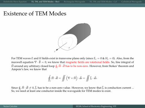
Existence of TEM Modes
For TEM waves E and H fields exist in transverse plane only (since Ez = 0 & Hz = 0). Also, from themaxwell equation ∇ ·~B = 0, we know that magnetic fields are rotational fields. So, line integral of~H around any arbitrary closed loop
¸C~H · ~dl has to be non-zero. However, from Stokes’ theorem and
Ampere’s law, we know that
˛C~H · ~dl =
¨ (∇× ~H
)· ~ds =
¨~Je · ~ds.
Since¸
C~H · ~dl 6= 0,~Je has to be a non-zero value. However, we know that~Je is conduction current ...
So, we need at least one conductor inside the waveguide for TEM modes to exist.
Vector Calculus EE208, School of Electronics Engineering, VIT
Helmholtz Wave Equation TE, TM, and TEM Modes – Rect Rectangular Waveguide TE, TM, and TEM Modes – Cyl Cylindrical Waveguide
Outline
1 Helmholtz Wave Equation
2 TE, TM, and TEM Modes – Rect
3 Rectangular Waveguide
4 TE, TM, and TEM Modes – Cyl
5 Cylindrical Waveguide
Vector Calculus EE208, School of Electronics Engineering, VIT
Helmholtz Wave Equation TE, TM, and TEM Modes – Rect Rectangular Waveguide TE, TM, and TEM Modes – Cyl Cylindrical Waveguide
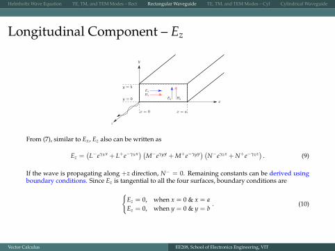
Longitudinal Component – Ez
From (7), similar to Ex, Ez also can be written as
Ez =(L−eγxx + L+e−γxx) (M−eγyy + M+e−γyy) (N−eγzz + N+e−γzz) . (9)
If the wave is propagating along +z direction, N− = 0. Remaining constants can be derived usingboundary conditions. Since Ez is tangential to all the four surfaces, boundary conditions are
{Ez = 0, when x = 0 & x = aEz = 0, when y = 0 & y = b
. (10)
Vector Calculus EE208, School of Electronics Engineering, VIT
Helmholtz Wave Equation TE, TM, and TEM Modes – Rect Rectangular Waveguide TE, TM, and TEM Modes – Cyl Cylindrical Waveguide
Longitudinal Component – Ez
First let us see the boundary conditions imposed by x = 0 and x = a. Since Ez = 0, when x = 0,
L− + L+ = 0⇒ L− = −L+ . (11)
Similarly Ez = 0, when x = a, so using the above equation one gets
L−eγxa + L+e−γxa = 0⇒ L+(e−γxa − eγxa) = 0⇒ sinh γxa = 0.
Hence, from the boundary conditions, we have γxa = sinh−1 (0) = j sin−1 (0) = jmπ, where m =0,±1,±2, . . . So,
γx=jmπ
a= 0 + jβx. (12)
Similarly, from boundary conditions at y = 0 and y = b, we can derive that
M− = −M+ and γy=jnπ
b= 0 + jβy, where n = 0,±1,±2, . . . (13)
Vector Calculus EE208, School of Electronics Engineering, VIT
Helmholtz Wave Equation TE, TM, and TEM Modes – Rect Rectangular Waveguide TE, TM, and TEM Modes – Cyl Cylindrical Waveguide
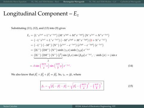
Longitudinal Component – Ez
Substituting (11), (12), and (13) into (9) gives
Ez =(L−eγxx + L+e−γxx) (M−eγyy + M+e−γyy) (N−eγzz + N+e−γzz)
=(−L+eγxx + L+e−γxx) (−M+eγyy + M+e−γyy) (0 + N+e−γzz)
=(−L+
) (−M+
) (N+) (
eγxx − e−γxx) (eγyy − e−γyy) (e−γzz)=(2L+
) (2M+
) (N+)
sinh (γxx) sinh(γyy)
e−γzz
=(2L+
) (2M+
) (N+) (
j2)︸ ︷︷ ︸
A
sin (βxx) sin(
βyy)
e−γzz, ∵ sinh (jx) = j sin x
= A sin(mπ
ax)
sin( nπ
by)
e−γzz. (14)
We also know that β2x + β2
y + β2z = β2
0. So, γz = jβz where
βz =√
β20 − β2
x − β2y =
√β2
0 −(mπ
a
)2−( nπ
b
)2. (15)
Vector Calculus EE208, School of Electronics Engineering, VIT
Helmholtz Wave Equation TE, TM, and TEM Modes – Rect Rectangular Waveguide TE, TM, and TEM Modes – Cyl Cylindrical Waveguide
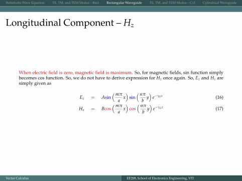
Longitudinal Component – Hz
When electric field is zero, magnetic field is maximum. So, for magnetic fields, sin function simplybecomes cos function. So, we do not have to derive expression for Hz once again. So, Ez and Hz aresimply given as
Ez = Asin(mπ
ax)
sin( nπ
by)
e−γzz (16)
Hz = Bcos(mπ
ax)
cos( nπ
by)
e−γzz (17)
Vector Calculus EE208, School of Electronics Engineering, VIT
Helmholtz Wave Equation TE, TM, and TEM Modes – Rect Rectangular Waveguide TE, TM, and TEM Modes – Cyl Cylindrical Waveguide
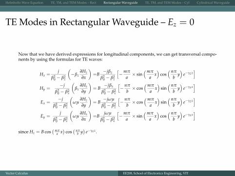
TE Modes in Rectangular Waveguide – Ez = 0
Now that we have derived expressions for longitudinal components, we can get transversal compo-nents by using the formulas for TE waves:
Hx =j
β20 − β2
z
(−βz
∂Hz
∂x
)=B
−jβz
β20 − β2
z
[−mπ
a× sin
(mπ
ax)
cos( nπ
by)
e−γzz]
Hy =−j
β20 − β2
z
(βz
∂Hz
∂y
)= B
−jβz
β20 − β2
z
[− nπ
b× cos
(mπ
ax)
sin( nπ
by)
e−γzz]
Ex =−j
β20 − β2
z
(ωµ
∂Hz
∂y
)= B
−jωµ
β20 − β2
z
[− nπ
b× cos
(mπ
ax)
sin( nπ
by)
e−γzz]
Ey =j
β20 − β2
z
(ωµ
∂Hz
∂x
)=B
jωµ
β20 − β2
z
[−mπ
a× sin
(mπ
ax)
cos( nπ
by)
e−γzz]
since Hz = B cos( mπ
a x)
cos( nπ
b y)
e−γzz.
Vector Calculus EE208, School of Electronics Engineering, VIT
Helmholtz Wave Equation TE, TM, and TEM Modes – Rect Rectangular Waveguide TE, TM, and TEM Modes – Cyl Cylindrical Waveguide
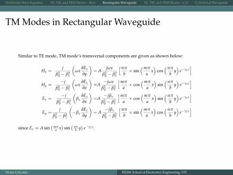
TM Modes in Rectangular Waveguide
Similar to TE mode, TM mode’s transversal components are given as shown below:
Hx =j
β20 − β2
z
(ωε
∂Ez
∂y
)= A
jωε
β20 − β2
z
[ nπ
b× sin
(mπ
ax)
cos( nπ
by)
e−γzz]
Hy =−j
β20 − β2
z
(ωε
∂Ez
∂x
)=A
−jωε
β20 − β2
z
[mπ
a× cos
(mπ
ax)
sin( nπ
by)
e−γzz]
Ex =−j
β20 − β2
z
(βz
∂Ez
∂x
)=A
−jβz
β20 − β2
z
[mπ
a× cos
(mπ
ax)
sin( nπ
by)
e−γzz]
Ey =j
β20 − β2
z
(−βz
∂Ez
∂y
)= A
−jβz
β20 − β2
z
[ nπ
b× sin
(mπ
ax)
cos( nπ
by)
e−γzz]
since Ez = A sin( mπ
a x)
sin( nπ
b y)
e−γzz.
Vector Calculus EE208, School of Electronics Engineering, VIT
Helmholtz Wave Equation TE, TM, and TEM Modes – Rect Rectangular Waveguide TE, TM, and TEM Modes – Cyl Cylindrical Waveguide
Modes in Rectangular Waveguide – IntuitiveExplanation
If you are fed up with the all the equations given in this PDF file, you may feel free to refer to much
simpler qualitative explanation given in another PDF file written on rectangular waveguides.
There, you can also find formulas for λg, ωcutoff, etc.
Vector Calculus EE208, School of Electronics Engineering, VIT
Helmholtz Wave Equation TE, TM, and TEM Modes – Rect Rectangular Waveguide TE, TM, and TEM Modes – Cyl Cylindrical Waveguide
Parallel Plate Waveguide
All the equations derived for rectangular waveguides can also be used for parallel plate
waveguide. After all, parallel plate waveguide is nothing but a rectangular waveguide with a→ ∞.
One major difference though is, in parallel plate waveguide in addition to TE and TM modes, TEM
modes also exist ... do you know why?
Vector Calculus EE208, School of Electronics Engineering, VIT
Helmholtz Wave Equation TE, TM, and TEM Modes – Rect Rectangular Waveguide TE, TM, and TEM Modes – Cyl Cylindrical Waveguide
Free Space Waveguide
Once again, the equations derived for rectangular waveguides can be used for free space too. It is
because, free space waveguide is nothing but a rectangular waveguide with a→ ∞ and b→ ∞ .
One major difference though is, similar to parallel plate waveguide, in free space, TEM modes also
exist ... do you know why?
Vector Calculus EE208, School of Electronics Engineering, VIT
Helmholtz Wave Equation TE, TM, and TEM Modes – Rect Rectangular Waveguide TE, TM, and TEM Modes – Cyl Cylindrical Waveguide
Outline
1 Helmholtz Wave Equation
2 TE, TM, and TEM Modes – Rect
3 Rectangular Waveguide
4 TE, TM, and TEM Modes – Cyl
5 Cylindrical Waveguide
Vector Calculus EE208, School of Electronics Engineering, VIT
Helmholtz Wave Equation TE, TM, and TEM Modes – Rect Rectangular Waveguide TE, TM, and TEM Modes – Cyl Cylindrical Waveguide
Maxwell’s Equations in Free Space
∇×~E = −jωµ~H
1ρ
(∂Ez
∂φ− ρ
∂Eφ
∂z
)= −jωµHρ(
∂Eρ
∂z− ∂Ez
∂ρ
)= −jωµHφ
1ρ
(∂(ρEφ
)∂ρ
−∂Eρ
∂φ
)= −jωµHz
∇× ~H = jωε~E
1ρ
(∂Hz
∂φ− ρ
∂Hφ
∂z
)= jωεEρ(
∂Hρ
∂z− ∂Hz
∂ρ
)= jωεEφ
1ρ
(∂(ρHφ
)∂ρ
−∂Hρ
∂φ
)= jωεEz
Eρ =−j
β20 − β2
z
(βz
∂Ez
∂ρ+
ωµ
ρ
∂Hz
∂φ
)Eφ =
−jβ2
0 − β2z
(βz
ρ
∂Ez
∂φ−ωµ
∂Hz
∂ρ
)Hρ =
jβ2
0 − β2z
(ωε
ρ
∂Ez
∂φ− βz
∂Hz
∂ρ
)Hφ =
−jβ2
0 − β2z
(ωε
∂Ez
∂ρ+
βz
ρ
∂Hz
∂φ
)
Once again, the above equations indicate the fact
that if longitudinal components Ez&Hz are
known, one can get all the transversal
components
Vector Calculus EE208, School of Electronics Engineering, VIT
Helmholtz Wave Equation TE, TM, and TEM Modes – Rect Rectangular Waveguide TE, TM, and TEM Modes – Cyl Cylindrical Waveguide
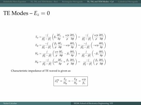
TE Modes – Ez = 0
Eρ =−j
β20 − β2
z
(βz
∂Ez
∂ρ+
ωµ
ρ
∂Hz
∂φ
)=
−jβ2
0 − β2z
(ωµ
ρ
∂Hz
∂φ
)Eφ =
−jβ2
0 − β2z
(βz
ρ
∂Ez
∂φ−ωµ
∂Hz
∂ρ
)=
−jβ2
0 − β2z
(−ωµ
∂Hz
∂ρ
)Hρ =
jβ2
0 − β2z
(ωε
ρ
∂Ez
∂φ− βz
∂Hz
∂ρ
)=
jβ2
0 − β2z
(−βz
∂Hz
∂ρ
)Hφ =
−jβ2
0 − β2z
(ωε
∂Ez
∂ρ+
βz
ρ
∂Hz
∂φ
)=
−jβ2
0 − β2z
(βz
ρ
∂Hz
∂φ
)
Characteristic impedance of TE waved is given as
ZTE0 =
Eρ
Hφ= −
Eφ
Hρ=
ωµ
βz
Vector Calculus EE208, School of Electronics Engineering, VIT
Helmholtz Wave Equation TE, TM, and TEM Modes – Rect Rectangular Waveguide TE, TM, and TEM Modes – Cyl Cylindrical Waveguide
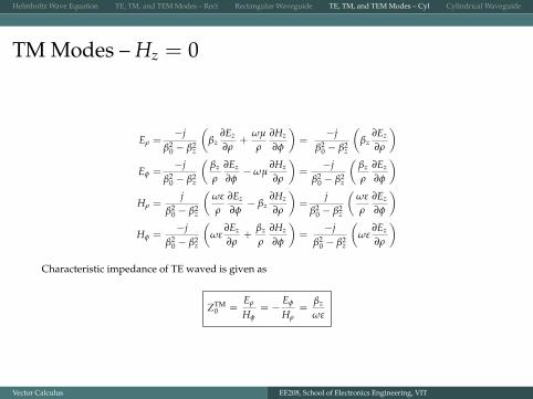
TM Modes – Hz = 0
Eρ =−j
β20 − β2
z
(βz
∂Ez
∂ρ+
ωµ
ρ
∂Hz
∂φ
)=
−jβ2
0 − β2z
(βz
∂Ez
∂ρ
)Eφ =
−jβ2
0 − β2z
(βz
ρ
∂Ez
∂φ−ωµ
∂Hz
∂ρ
)=
−jβ2
0 − β2z
(βz
ρ
∂Ez
∂φ
)Hρ =
jβ2
0 − β2z
(ωε
ρ
∂Ez
∂φ− βz
∂Hz
∂ρ
)=
jβ2
0 − β2z
(ωε
ρ
∂Ez
∂φ
)Hφ =
−jβ2
0 − β2z
(ωε
∂Ez
∂ρ+
βz
ρ
∂Hz
∂φ
)=
−jβ2
0 − β2z
(ωε
∂Ez
∂ρ
)
Characteristic impedance of TE waved is given as
ZTM0 =
Eρ
Hφ= −
Eφ
Hρ=
βz
ωε
Vector Calculus EE208, School of Electronics Engineering, VIT
Helmholtz Wave Equation TE, TM, and TEM Modes – Rect Rectangular Waveguide TE, TM, and TEM Modes – Cyl Cylindrical Waveguide
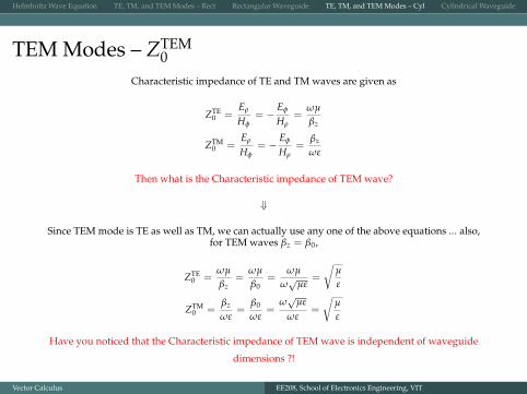
TEM Modes – ZTEM0
Characteristic impedance of TE and TM waves are given as
ZTE0 =
Eρ
Hφ= −
Eφ
Hρ=
ωµ
βz
ZTM0 =
Eρ
Hφ= −
Eφ
Hρ=
βz
ωε
Then what is the Characteristic impedance of TEM wave?
⇓
Since TEM mode is TE as well as TM, we can actually use any one of the above equations ... also,for TEM waves βz = β0,
ZTE0 =
ωµ
βz=
ωµ
β0=
ωµ
ω√
µε=
õ
ε
ZTM0 =
βz
ωε=
β0
ωε=
ω√
µε
ωε=
õ
ε
Have you noticed that the Characteristic impedance of TEM wave is independent of waveguide
dimensions ?!
Vector Calculus EE208, School of Electronics Engineering, VIT
Helmholtz Wave Equation TE, TM, and TEM Modes – Rect Rectangular Waveguide TE, TM, and TEM Modes – Cyl Cylindrical Waveguide
Outline
1 Helmholtz Wave Equation
2 TE, TM, and TEM Modes – Rect
3 Rectangular Waveguide
4 TE, TM, and TEM Modes – Cyl
5 Cylindrical Waveguide
Vector Calculus EE208, School of Electronics Engineering, VIT
Helmholtz Wave Equation TE, TM, and TEM Modes – Rect Rectangular Waveguide TE, TM, and TEM Modes – Cyl Cylindrical Waveguide
Helmholtz Wave Equation - Cylindrical CoordinateSystem
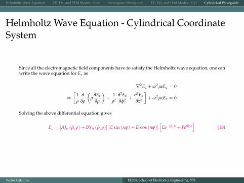
Since all the electromagnetic field components have to satisfy the Helmholtz wave equation, one canwrite the wave equation for Ez as
∇2Ez + ω2µεEz = 0
⇒[
1ρ
∂
∂ρ
(ρ
∂Ez
∂ρ
)+
1ρ2
∂2Ez
∂φ2 +∂2Ez
∂z2
]+ ω2µεEz = 0.
Solving the above differential equation gives
Ez = [AJn (βcρ) + BYn (βcρ)] [C sin (nφ) + D cos (nφ)][Ee−jβzz + Fejβzz
](18)
Vector Calculus EE208, School of Electronics Engineering, VIT
Helmholtz Wave Equation TE, TM, and TEM Modes – Rect Rectangular Waveguide TE, TM, and TEM Modes – Cyl Cylindrical Waveguide
Longitudinal Components – Ez & Hz
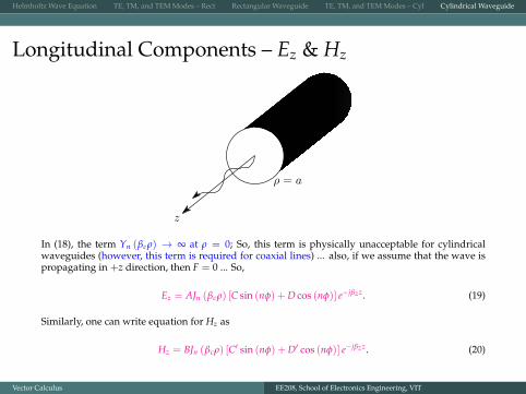
In (18), the term Yn (βcρ) → ∞ at ρ = 0; So, this term is physically unacceptable for cylindricalwaveguides (however, this term is required for coaxial lines) ... also, if we assume that the wave ispropagating in +z direction, then F = 0 ... So,
Ez = AJn (βcρ) [C sin (nφ) + D cos (nφ)] e−jβzz. (19)
Similarly, one can write equation for Hz as
Hz = BJn (βcρ) [C′ sin (nφ) + D′ cos (nφ)] e−jβzz. (20)
Vector Calculus EE208, School of Electronics Engineering, VIT
Helmholtz Wave Equation TE, TM, and TEM Modes – Rect Rectangular Waveguide TE, TM, and TEM Modes – Cyl Cylindrical Waveguide
Cylindrical Waveguide – TE modes
Eρ =−j
β20 − β2
z
(ωµ
ρ
∂Hz
∂φ
)= B
−jβ2
0 − β2z
[ωµ
ρ
[Jn (βcρ) [nC′ cos (nφ)− nD′ sin (nφ)] e−jβzz
]]Eφ =
−jβ2
0 − β2z
(−ωµ
∂Hz
∂ρ
)=B
−jβ2
0 − β2z
[−ωµ
[βcJ′n (βcρ) [C′ sin (nφ) + D′ cos (nφ)] e−jβzz
]]Hρ =
jβ2
0 − β2z
(−βz
∂Hz
∂ρ
)= B
jβ2
0 − β2z
[−βz
[βcJ′n (βcρ) [C′ sin (nφ) + D′ cos (nφ)] e−jβzz
]]Hφ =
−jβ2
0 − β2z
(βz
ρ
∂Hz
∂φ
)= B
−jβ2
0 − β2z
[βz
ρ
[Jn (βcρ) [nC′ cos (nφ)− nD′ sin (nφ)] e−jβzz
]]
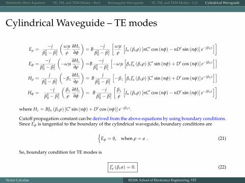
where Hz = BJn (βcρ) [C′ sin (nφ) + D′ cos (nφ)] e−jβzz.
Cutoff propagation constant can be derived from the above equations by using boundary conditions.Since Eφ is tangential to the boundary of the cylindrical waveguide, boundary conditions are
{Eφ = 0, when ρ = a . (21)
So, boundary condition for TE modes is
J′n (βca) = 0. (22)
Vector Calculus EE208, School of Electronics Engineering, VIT
Helmholtz Wave Equation TE, TM, and TEM Modes – Rect Rectangular Waveguide TE, TM, and TEM Modes – Cyl Cylindrical Waveguide
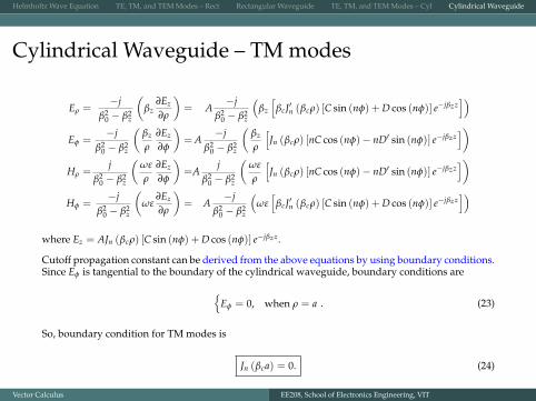
Cylindrical Waveguide – TM modes
Eρ =−j
β20 − β2
z
(βz
∂Ez
∂ρ
)= A
−jβ2
0 − β2z
(βz
[βcJ′n (βcρ) [C sin (nφ) + D cos (nφ)] e−jβzz
])Eφ =
−jβ2
0 − β2z
(βz
ρ
∂Ez
∂φ
)= A
−jβ2
0 − β2z
(βz
ρ
[Jn (βcρ) [nC cos (nφ)− nD′ sin (nφ)] e−jβzz
])Hρ =
jβ2
0 − β2z
(ωε
ρ
∂Ez
∂φ
)=A
jβ2
0 − β2z
(ωε
ρ
[Jn (βcρ) [nC cos (nφ)− nD′ sin (nφ)] e−jβzz
])Hφ =
−jβ2
0 − β2z
(ωε
∂Ez
∂ρ
)= A
−jβ2
0 − β2z
(ωε[
βcJ′n (βcρ) [C sin (nφ) + D cos (nφ)] e−jβzz])
where Ez = AJn (βcρ) [C sin (nφ) + D cos (nφ)] e−jβzz.
Cutoff propagation constant can be derived from the above equations by using boundary conditions.Since Eφ is tangential to the boundary of the cylindrical waveguide, boundary conditions are
{Eφ = 0, when ρ = a . (23)
So, boundary condition for TM modes is
Jn (βca) = 0. (24)
Vector Calculus EE208, School of Electronics Engineering, VIT
![dosya.marmara.edu.trdosya.marmara.edu.tr/tf/tem/staj/EK-6.docx · Web view[ EK-6: ÖRNEK STAJ RAPORU (TEM 300 /TEM3000) ] TEKSTİL MÜHENDİSLİĞİ BÖLÜMÜ TEM 3 00 / TEM 3 000](https://img.pdfslide.us/doc/110x75/5e40cd8392c8432d520232c3/dosya-web-view-ek-6-rnek-staj-raporu-tem-300-tem3000-tekstl-moehendsl.jpg)