Ryozo Himino - 財務省 Himino Vice Commissioner ... ble, ii) added layers of qualitative guidance as the bubble grew, ... Japan’s banking crisis in the 1990s and the Global Finan-

253

Japanese responses to asset price bubbles: comparison with the U.S.＊

Ryozo HiminoVice Commissioner for International Affairs, Financial Services Agency, Japan

AbstractIt is widely believed that the Japanese response to the boom and the bust in the late

1980s and early 1990s was too little and too late, while that of the US in the 2000 was deci-sive and timely. Though such may have been the case with the bailing out of large banks and the recognition and resolution of bad assets, the monetary policy responses in Japan and the U.S. before and after the real estate price peaks closely resemble each other in their i) size and timing of tightening and easing, ii) deviation from the Taylor targets and iii) responses to asset price impulse. Prudential policies in Japan and the US also were common in that they i) started with qualitative guidance on real estate lending in the early phases of the bub-ble, ii) added layers of qualitative guidance as the bubble grew, and iii) stepped into quanti-tative guidance only after the initial signs of peaking-out.

Though the Japanese authorities are believed to have “leaned” to prick the bubble while the U.S. authorities argued against leaning and advocated “cleaning up” the mess after the bust, their behavior did not differ much. Intention, action and effects staggered with each other and both monetary and prudential policies in Japan and in the U.S. lagged behind the real estate price moves and may have deepened the bust. Timeliness of the policy responses may matter more than how they are motivated, explained or labelled: clean or lean, micro- or macro-prudential.

　 Keywords: asset price bubbles, monetary policy, prudential policy, clean, lean　 JEL Classification: N25, E52, G01, G28

I. Objectives

It is often argued that Japan’s policy responses to the asset price bubbles are responsible for the country’s ensuing economic stagnation.

Some maintain that policy actions were ill-timed. Bernanke and Gertler (1999) and Oki-na, Shirakawa and Shiratsuka (2001) argue that the measures to contain the bubbles should have started earlier, while Hamada, Kashyap and Weinstein (2011) claim that the authorities

＊ Parts of this article were presented at the conference “Next Steps for Macroprudential Policy” organized by the School of International and Public Affairs of Columbia University and the IESE Business School of the University of Navarra and held in New York in November 2015 and at the conference “Financial Deregulation in China and Japan: The Risk and the Chances” organized by the Meiji University and the Chinese Academy of Social Sciences and held in Tokyo in November 2014. The au-thor appreciates the comments given at the conferences. He also has benefited from discussions with Messrs. Toshitaka Sekine (Bank of Japan), Hiroshi Tsubouchi (Cabinet Office) and Yoshihiko Uchida (Financial Services Agency). The views expressed in the article are the author’s and are not those of the Financial Services Agency. All the factual descriptions are based on pub-lic information.

Policy Research Institute, Ministry of Finance, Japan, Public Policy Review, Vol.12, No.2, March 2016

were slow to recognize the collapse of the bubbles and to shift from tightening to easing.Some maintain that policy actions were ill-calibrated. Okada and Hamada (2009) accuse

the measures for containing the bubbles of being excessive, while Ahearne et al. (2002) ar-gues that more aggressive easing after the collapse would have saved Japan from deflation.

Others maintain that inappropriate policy tools were deployed. Muramatsu and Okuno (2002) criticize the use of a prudential tool, while Bernanke (Federal Reserve Bank of Kan-sas City, 2003, p. 226) argues that monetary policy should not have been used to prick the bubble.

This article tries to find whether the Japan’s policy responses were ill-timed, ill-calibrat-ed or ill-composed and to draw lessons from Japan’s experience.

The article focuses on the period between 1986, the year asset prices started to hike, and 1992, the year the collapse of the bubble had become evident to anyone’s eyes. It does not deal with the 1986 shift in Japan’s growth strategy from an export driven one to a domestic demand driven one, though it may have contributed to the emergence of the asset price bub-bles. Nor does it deal with the resolution of non-performing loans and insolvent banks after 1992, though it may have affected the depth and the length of the downturn.

Section II is a brief review of the debates since the Great Depression until the Global Fi-nancial Crisis on optimum policy responses to bubbles. Section III provides overviews of the sequences of asset price moves and policy responses in Japan. Section IV reviews mone-tary policy measures taken, and Section V reviews prudential policy ones and compares them with those taken in the U.S. in the 2000s. Section VI reviews tax, land and fiscal poli-cy measures taken in Japan. Section VII tries to find whether Japan’s policy responses were ill-timed, ill-calibrated or ill-composed. Section VIII summarizes the lessons from the expe-rience of Japan and the U.S.

II. “Clean” or “lean”

Bubbles, or unsustainable expansion of financial imbalances accompanied by unsustain-able asset price hikes, have repeatedly plagued mankind. The U.S. Great Depression, the Japanese boom and bust around 1990, and the Global Financial Crisis in the 2000s have all prompted debate on optimum policy responses to bubbles. Almost 100 years of debates, however, have not yet resulted in a consensus.

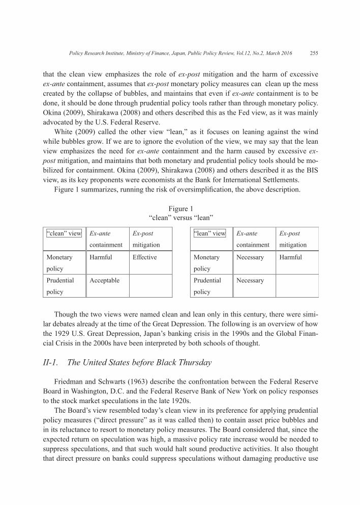
Policy responses to bubbles can be classified by their aims and means. By aim, they can be classified into i) ex-ante measures to contain the boom and ii) ex-post measures to miti-gate the shocks of the bust. With regard to means, two categories of policy tools have main-ly been discussed: i) monetary policy tools (such as changes in policy rates and quantitative easing) and ii) prudential policy tools (such as moral suasion, guidance on risk management, lending limits, bank capital adequacy regulations, and loan-to-value limits).

Two views can be distinguished by their preferred aims and means.White (2009) called one of them “clean,” as it focuses on the cleaning up of the mess

created by the collapse of bubbles. If we are to ignore nuances and variations, we may say

254 R Himino / Public Policy Review

255

that the clean view emphasizes the role of ex-post mitigation and the harm of excessive ex-ante containment, assumes that ex-post monetary policy measures can clean up the mess created by the collapse of bubbles, and maintains that even if ex-ante containment is to be done, it should be done through prudential policy tools rather than through monetary policy. Okina (2009), Shirakawa (2008) and others described this as the Fed view, as it was mainly advocated by the U.S. Federal Reserve.

White (2009) called the other view “lean,” as it focuses on leaning against the wind while bubbles grow. If we are to ignore the evolution of the view, we may say that the lean view emphasizes the need for ex-ante containment and the harm caused by excessive ex-post mitigation, and maintains that both monetary and prudential policy tools should be mo-bilized for containment. Okina (2009), Shirakawa (2008) and others described it as the BIS view, as its key proponents were economists at the Bank for International Settlements.

Figure 1 summarizes, running the risk of oversimplification, the above description.

Figure 1“clean” versus “lean”

Though the two views were named clean and lean only in this century, there were simi-lar debates already at the time of the Great Depression. The following is an overview of how the 1929 U.S. Great Depression, Japan’s banking crisis in the 1990s and the Global Finan-cial Crisis in the 2000s have been interpreted by both schools of thought.

II-1. The United States before Black Thursday

Friedman and Schwarts (1963) describe the confrontation between the Federal Reserve Board in Washington, D.C. and the Federal Reserve Bank of New York on policy responses to the stock market speculations in the late 1920s.

The Board’s view resembled today’s clean view in its preference for applying prudential policy measures (“direct pressure” as it was called then) to contain asset price bubbles and in its reluctance to resort to monetary policy measures. The Board considered that, since the expected return on speculation was high, a massive policy rate increase would be needed to suppress speculations, and that such would halt sound productive activities. It also thought that direct pressure on banks could suppress speculations without damaging productive use


of funds.The New York Fed’s view, on the other hand, resembled today’s “lean” view in that it

allocated monetary policy to ex-ante containment: The bank believed that speculative use of funds could not be distinguished from productive use, that it was not possible to suppress only the former, and that speculation could be contained only by monetary policy. It was re-luctant to use “direct pressure” as it believed that “once member banks got the impression that they could not get money at any price, if needed, it might result in a very critical situa-tion.”

The Board published a statement warning against the growth of speculative security loans and criticized the New York Fed for neglecting the task of exerting direct pressure. On the other hand, since February 1929 the New York Fed requested 10 times that the Board approve a discount rate increase, only to be rejected each time. The request was approved in August but the effect was mitigated by the reduction in bill rates, which was done to meet productive fund demand.

Friedman and Schwartz (1963) disapprove of both the prudential and the monetary poli-cy measures taken. They maintain that the Fed resorted to direct pressure to “demonstrate to itself and others that it was taking some action to meet clear and pressing problems” though it knew or at least strongly suspected that it might be in vain. And for Friedman and Schwartz (1963), the monetary policy measures taken were “restrictions that were clearly too easy to stem the bull market and almost surely too tight to permit the continued expan-sion of business activity without severe downward pressure on prices.”

Then, which way should the Fed have gone, easier or tighter?Galbraith (1954) seems to believe that it should have gone tighter. He explains as fol-

lows why it did not: “A bubble can easily be punctuated. But to incise it with a needle so that it subsides gradually is a task of no small delicacy. . . . The real choice was between an immediate and deliberately engineered collapse and a more serious disaster later on. Some-one would certainly be blamed for the ultimate collapse when it came. There was no ques-tion whatever as to who would be blamed should the boom be deliberately deflated.”

Bernanke (2002), on the other hand, considers that the Fed went too tight: Although “there was not the slightest hint of inflation,” the Federal Reserve made “antispeculative” policy tightening and “the economy responded in the way that the monetary theory of the Great Depression would predict.”

Both learning from the experience of the Great Depression, Galbraith draws lean-style lessons and Bernanke draws clean ones.

II-2. Japan’s “failure”

As was the case with the Great Depression, Japan’s “failure” in the 1990s was interpret-ed in two opposite ways. For example, at the Jackson Hall conference in 2003, where de-bates on Borio and White (2004) were held, proponents of clean and lean both cited Japan as a poster child of their own views. (Federal Reserve Bank of Kansas City, 2003, pp.226–


257

229)Supporting the lean arguments in Borio and White (2004), Michale Mussa commented,

“It seems to me that the poster child for discussing why monetary policy should, in selected instances, pay serious attention to asset-price distortions on the upside is not the United States in the late 1990s. It is Japan at the end of the 1980s. . . . Looking at a CPI inflation rate that remained very low saw an enormous explosion of asset prices, real estate prices, and enormous growth of credit. If that price bubble collapsed, there was going to be serious macroeconomic problems.”

Ben Bernanke did not agree: “I am astonished by Michael Mussa citing Japan as a post-er child for this paper. It is just the opposite. . . . The only place that monetary policy played a role was that in 1989 it intentionally tried to prick the bubble. It raised interest rates sharp-ly in precisely the kind of program that is being suggested here. It did succeed in pricking the bubble. Asset prices collapsed and they had a 14-year depression.”

Bernanke and Gertler (1999) argued that had the Bank of Japan properly focused on the traditional targets of monetary policy (inflation and output), it would have raised the policy rate from around 4% to around 8% in 1988 and would have successfully prevented the asset price bubbles. As shown by Okina and Shiratsuka (2002), this finding was biased by a fail-ure to account for the effect of the VAT introduced in 1989 on CPI, but has strengthened the clean view belief that monetary policy need not make any additional prick-the-bubble reac-tions.

Ahearne et al. (2002) showed a simulation result showing that if the Bank of Japan had lowered short-term interest rates by a further 250 basis points at any time between 1991 and early-1995, deflation could have been avoided. This finding also worked to strengthen the clean view belief that ex-post mitigation can clean-up any mess in the wake of collapses of bubbles.

II-3. The Global Financial Crisis in the 2000s

The Global Financial Crisis in the 2000s resulted in changes in nuances of both schools but has not resolved the dispute yet.

The clean view, which formed the leading policy framework during the period leading up to the Global Financial Crisis but which failed to prevent the crisis by ex-post mitigation, was expressed in a more nuanced manner in the wake of the crisis. As time goes by, howev-er, it seems that the pre-crisis wording is being revived. Mishkin (2011) already declared that “much of the science of monetary policy remains intact.” Yellen (2014) may remind us of the pre-crisis Fed remarks as well as the Board views in 1929: “I will argue that monetary policy faces significant limitations as a tool to promote financial stability: Its effects on fi-nancial vulnerabilities, such as excessive leverage and maturity transformation, are not well understood and are less direct than a regulatory or supervisory approach; in addition, efforts to promote financial stability through adjustments in interest rates would increase the vola-tility of inflation and employment. As a result, I believe a macroprudential approach to su-


pervision and regulation needs to play the primary role.”The post-crisis lean view distinguishes two phases in ex-post mitigation, the crisis man-

agement phase and the recovery phase. The view now admits the role monetary policy can play in the former phase, but emphasizes the risk of relying on monetary policy in the latter. According to Borio (2014), “The priority in crisis management is to shore up confidence. In this phase, it is natural to use monetary policy aggressively. . . . The priority in crisis resolu-tion, by contrast, is to repair the balance sheets of the financial and non-financial sectors. . . . There are grounds to believe that in the crisis resolution phase monetary policy is likely to be less effective than in a normal recession.”

In the following, we will look at Japan’s experience and examine how it compares with the two views.

III. Timeline of asset price moves and policy responses in Japan

This section provides an overview of the developments in Japan around the time of the bubble collapses.

III-1. Bubble collapse sequences in Japan and the U.S.

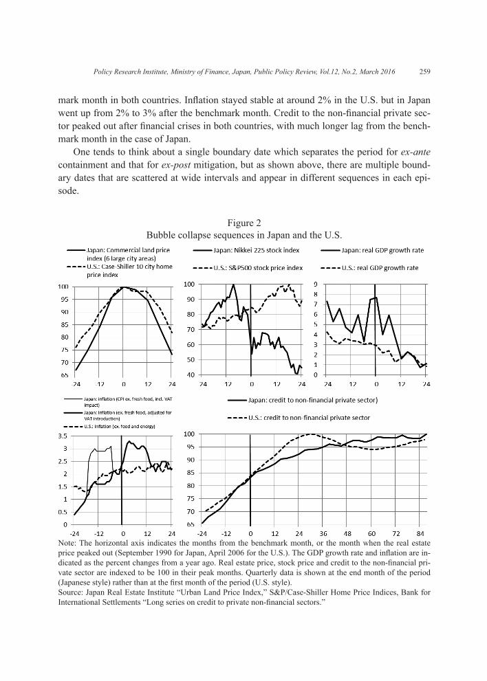
The sequences of the peaks of various asset prices and the macro-economic indicators differed between Japan in the 1990s and the U.S. in the 2000s.

In the case of Japan, the stock price peak preceded the land price peak. The stock price peak came first (December 1989), followed nine months later by the large city land price peak (September 1990), and then further five months later by the business cycle peak (Feb-ruary 1991). The peak in credit in the non-financial private sector came seven years after, in the wake of the systemic banking crisis.

On the other hand, the home price peak preceded the stock price peak in the U.S. The home price indices peaked out in April 2006,1 followed 18 months later by the stock price peak in October 2007, and then further two months later by the business cycle peak in De-cember 2007. Credit to the non-financial private sector peaked out in September 2008 when Lehman Brothers failed.

The timeliness of policy responses looks different depending on whether one uses the stock price moves as a benchmark or those of the real estate price. In this paper we focus on the real estate prices, as they had a much larger impact on the economy and the financial system than the stock prices both in Japan and in the U.S. Figure 2 uses the peak months of the real estate prices as the benchmark months (month zero) and compares the moves of as-set prices and macroeconomic indices. The GDP growth decelerated from around the bench- 1 Seasonally adjusted series of the Case-Shiller 10 city and 20 city home price indices and the First American Core Logic house price index peaked in April 2006; non-seasonally adjusted series of the Case-Shiller 10 city index in June 2006; and, non-seasonally adjusted series of the Case-Shiller 20 city index in July 2006. All of them peaked far in advance of the stock price peak and the business cycle peak.


259

mark month in both countries. Inflation stayed stable at around 2% in the U.S. but in Japan went up from 2% to 3% after the benchmark month. Credit to the non-financial private sec-tor peaked out after financial crises in both countries, with much longer lag from the bench-mark month in the case of Japan.

One tends to think about a single boundary date which separates the period for ex-ante containment and that for ex-post mitigation, but as shown above, there are multiple bound-ary dates that are scattered at wide intervals and appear in different sequences in each epi-sode.

Figure 2Bubble collapse sequences in Japan and the U.S.

Note: The horizontal axis indicates the months from the benchmark month, or the month when the real estate price peaked out (September 1990 for Japan, April 2006 for the U.S.). The GDP growth rate and inflation are in-dicated as the percent changes from a year ago. Real estate price, stock price and credit to the non-financial pri-vate sector are indexed to be 100 in their peak months. Quarterly data is shown at the end month of the period (Japanese style) rather than at the first month of the period (U.S. style).Source: Japan Real Estate Institute “Urban Land Price Index,” S&P/Case-Shiller Home Price Indices, Bank for International Settlements “Long series on credit to private non-financial sectors.”


III-2. Policy response timeline

How then did the Japanese authorities respond to the developments in the asset price and the economy?

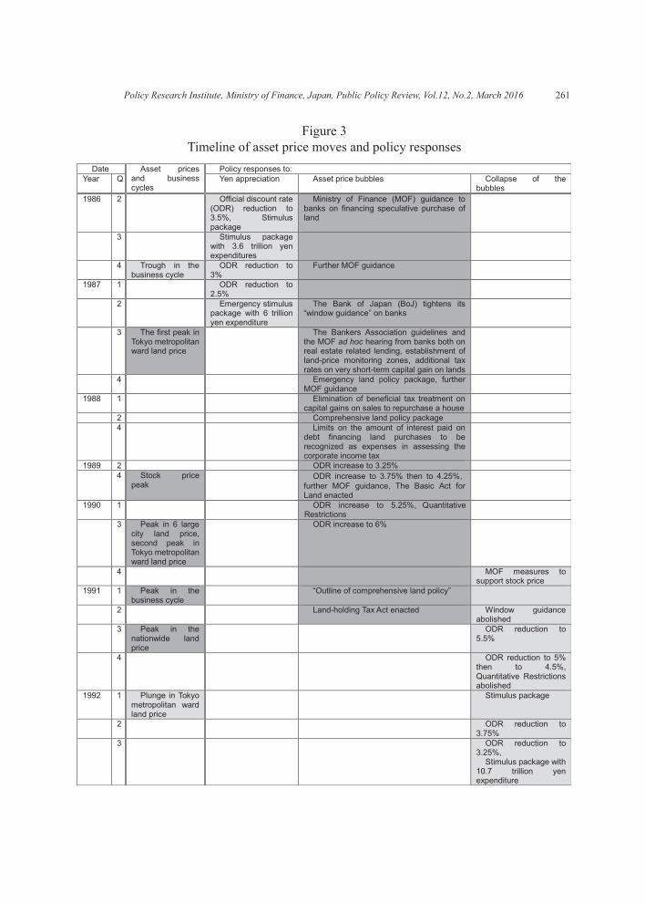
Figure 3 is a chronology of asset price and business cycle developments (the third col-umn) and policy responses to them. The key policy objective shifted from the mitigation of the depressive effects of the appreciation of the yen (the fourth column of Figure 3 lists measures taken in this regard) to the correction of distributional distortions arising from the land price hike (the fifth column) then to the mitigation of the depressive effects of the col-lapse of the bubbles (the sixth column).

The key policy objectives, however, shifted with overlapping periods and the authorities sometimes had to pursue two opposing objectives at the same time.

For example, from 1986 to the first half of 1987, the primary policy objective was to limit the trade surplus to abate the trade war with the U.S., to protect the export industry from the strong yen, and mitigate the depressive effects of the strong yen. But the govern-ment also tried to contain the land price boom, as it was considered to be depriving many from the opportunity to have their own home and causing distributional distortion. Pruden-tial policy measures (administrative guidance against financing real estate speculation) start-ed as early as 1986.

From the latter half of 1987 to 1988, the fear of renewed appreciation of the yen pre-vented the authorities from activating monetary policy to contain the real estate and stock market booms. Only land policy, tax policy, and prudential policy measures were mobilized for the purpose.

In 1989, the appreciation of the yen since 1985 finally reversed and the monetary policy found room for tightening. Land price hikes had spread from the largest cities to all over Ja-pan, turning the matter into a political priority. The policy authorities started to put more weighting on land than on the yen. By that time, three years had passed since the start of the bubble.

In 1990, stock prices plummeted but the land price continued to rise. The authorities got opposing signals from the asset markets but they focused on the signal from the real estate market, mainly due to the political and social anger at what then was called “the crazy land price.” Moreover, the economy was still strong.

The official discount rate cut in July 1991 marked a shift in policy priority from the con-tainment of the land boom to the mitigation of the effects of the bust. The shift was made one and a half years after the stock price plunge, almost one year after the large city land price peak and a half year after the business cycle peak. After that, the official discount rate was reduced and fiscal stimulus was added repeatedly.

As discussed above, monetary, prudential, tax, land and fiscal policy measures were all mobilized during the period of the boom and bust. In the following sections, we will look at how the authorities chose the timing, the calibration, and the tools of policy responses.


261

Figure 3Timeline of asset price moves and policy responses


IV. Monetary policy

IV-1. Japan’s experience

The Bank of Japan kept its official discount rate at a post-war low of 2.5% for two years and three months while the asset price bubbles continued to expand. Then the appreciation of the yen had been reversed and it raised the rate three times in a half year, in May, October and December 1989. The free fall in stock price commenced in January 1990 but the Bank further raised the rate in March and August to 6%. Rate increases were repeated five times and amounted to 350 basis points in a year and three months. The actions were interpreted to show the Bank’s strong resolve to prick the bubbles.

The stock market continued to tumble but the Bank of Japan kept the rate at 6% for al-most a year. It reversed course in July 1997 and made rate cuts six times during the ensuing one year and seven months until February 1993, cutting 350 basis points in aggregate to 2.5%, the level before its prick-the-bubbles operation.

Some argue in hindsight that had the Bank of Japan i) tightened earlier, ii) tightened more moderately, iii) eased earlier, or iv) eased more aggressively, the aftermath of the col-lapse of the bubble would have been less painful. There were, however, reasons that pre-vented the Bank from doing so.

i)　Why was tightening not commenced earlier than May 1989?The yen started to depreciate in early 1989 and plunged in mid-May, and in end-May the

Bank of Japan started to tighten. The sequence implies that it was the strong yen that pre-vented earlier tightening. Satoshi Sumita, the governor of the Bank of Japan from 1984 to 1989, later recounted, “If we had tightened, the yen would have appreciated . . . . The politi-cal sector, the industry, all were unanimous in demanding no stronger yen. Tightening was difficult to do.” (Nikkei, 2000)

The monetary policy dilemma between a strong currency and rising asset prices is not unique to Japan in 1980s. Fisher (2014) reports that house prices in Israel went up signifi-cantly after 2008 but the Bank of Israel refrained from tightening as exports were critical to the country’s growth. Switzerland in the 2010s faced the same dilemma.

ii)　Why was the tightening so aggressive?The national priority had shifted from the yen to land in 1990. Takenaka (2005) argues

that the land price had become a nation-wide political priority in 1990 as the speculation spread from Tokyo to all of Japan. Yasushi Mieno, who succeeded Sumita as Governor in December 1989, stated at his inaugural press conference, “The nation is frustrated with the increasing wealth disparity among them resulting from the land and stock price boom.” Right after his inauguration, the Finance Minister demanded that the Governor cancel the planned rate increase but the Governor did not take heed. A Bank of Japan high official is


263

said to have declared to bankers, “We will tighten more till we kill the bubbles.” (Nikkei, 2000)

The Wall Street Journal (1993) reports Governor Mieno’s remark: “The giddy expansion of the late 1980s ‘undermined the stability and soundness of Japanese society by weakening the ethos of labor, the notion of working by the sweat of your brow.’ The boom, he contends, hastened ‘a decline in morals’ and fostered ‘inequalities in the distribution of wealth.’”

Governor Mieno was seen as a defender of central bank independence and a brave bub-ble buster. The public applauded him comparing him to a champion-of-justice police com-missioner in 18th century Japan, the protagonist of a popular novel series.

iii)　Why was easing not started earlier than July 1991?The sequence of events was as follows: the stock price peak (December 1989), the six

large city land price peak (September 1990), the inflation rate peak (December 1990), the business cycle peak (February 1991), the monetary policy turnaround (July 1991) and the nationwide land price peak (September 1991). The monetary policy turning point was not behind the most lagged indicator but far behind the leading indicators. The Minister for Eco-nomic Planning criticized the Bank’s tight monetary policy already in December 1990, and in retrospect we may say that he knew better.

But public opinion continued to demand that the Bank play the role of bubble buster. As late as autumn 1991, major newspapers advocated, “Let’s exterminate the land price bub-ble” (Asahi), “Bubble land prices shall not stay” (Mainichi), “Don’t loosen land policy” (Yomiuri), “We cannot be relieved by moderated land prices” (Nikkei), and “Why rush to ease monetary policy?” (Tokyo) (quoted in Nishimura, 1999). The six large city land price index had a bigger bearing on the economy, but the nationwide index had a much bigger po-litical implication.

iv)　Why was easing not more aggressive?Ahearne et al. (2002) argued a further 250 basis point cut would have saved Japan from

deflation, but their recommendation only came 10 years after. No one at the time foresaw the ensuing depression, deflation and banking crisis, and the range of views on the appropri-ate speed of easing was rather limited.

The leading contemporaneous advocate of aggressive easing was Vice President Kana-maru of the ruling Liberal Democratic Party, who in February 1991 commented that, “even by chopping off the head of the Bank of Japan governor,” a further 50 basis point cut had to be attained. The strong wording suggests that Kanamaru knew what Japan needed ten years before Ahearne et al. (2002) found it. One month later, the Bank of Japan reduced its policy rate by 75 basis points. It is said that the Bank had been in the process of a rate cut at the time of Kanamaru’s remarks but that it chose to do so at a slightly different timing and size to protect the optics of central bank independence (Kamikawa, 2002).

The monetary policy moved largely in line with the shifts in public priorities from miti-gating the strong yen, to containing the land price boom and then to mitigating the effects of


the bust. Governor Mieno, who took away the punch bowl while the party got going, was applauded as a champion of justice. When the effects of the land price bust manifested itself, however, the public changed their views and started to blame him for bringing in the crisis.

IV-2. Comparison with the U.S. experience

Below we show that the monetary policy responses in Japan and the U.S. before and af-ter the real estate price peaks closely resembled each other in their i) size and timing of tightening and easing, ii) deviation from the Taylor targets and iii) responses to output, asset price and foreign exchange impulses.

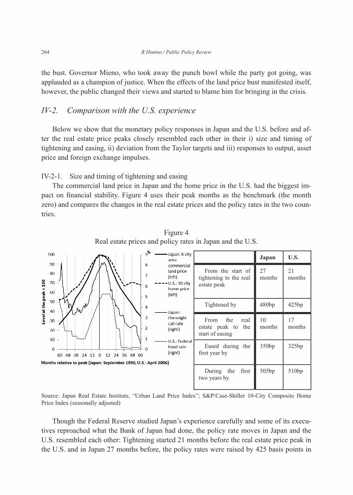
IV-2-1. Size and timing of tightening and easingThe commercial land price in Japan and the home price in the U.S. had the biggest im-

pact on financial stability. Figure 4 uses their peak months as the benchmark (the month zero) and compares the changes in the real estate prices and the policy rates in the two coun-tries.

Source: Japan Real Estate Institute, “Urban Land Price Index”; S&P/Case-Shiller 10-City Composite Home Price Index (seasonally adjusted)

Figure 4Real estate prices and policy rates in Japan and the U.S.

Though the Federal Reserve studied Japan’s experience carefully and some of its execu-tives reproached what the Bank of Japan had done, the policy rate moves in Japan and the U.S. resembled each other: Tightening started 21 months before the real estate price peak in the U.S. and in Japan 27 months before, the policy rates were raised by 425 basis points in


265

the U.S. and 480 basis points in Japan, easing started 17 months after the real estate price peak in the U.S. and 10 months in Japan, and the rates were cut by 325 basis points in the first year in the U.S. and 350 basis points in Japan, and by 510 basis points during the first two years in the U.S. and 505 basis points in Japan. The Bank of Japan started to tighten and ease more promptly, and tightened and eased as aggressively as the Federal Reserve. This defies the view that the Bank of Japan did too little, too late while the Federal Reserve acted decisively and timely.

As the sequence of the stock price peak and the real estate price peak occurred in reverse in the U.S. and Japan, if we use the stock price peak as the benchmark months as Hamada, Kashyap and Weinstein (2011) do, the Bank of Japan would look much slower in tightening and easing than the Federal Reserve. However, it was the real estate price boom, not the stock prime boom, which brought the financial crises to the two countries.

VI-2-2. Deviation from the Taylor targetsThen, were the trajectories of these policy rates consistent with the traditional monetary

policy targets (inflation and output) at the time or were they the result of additional tighten-ing or easement in response to asset price fluctuations? To answer this question, in the fol-lowing we will compare the actual policy rates with what the Taylor rule, or a standard poli-cy rule which refers only to inflation and output gaps, would suggest as the target levels.

Taylor (1993) proposed that the monetary policy under the floating exchange regime should put equal weight on two gaps: i) the gap between the inflation and the inflation target and ii) the GDP gap. He maintained that formula (1) can explain the U.S. federal fund rate moves during the five years preceding the publication of the paper, from 1987 to 1992.

　　i=（π+2）+0.5y+0.5（π－2） (1)

where “i” stands for the policy rate level, π the inflation rate over the last four quarters, and “y” GDP gap—all represented as percentages. The “2” included in the first term (π+2) rep-resents the real equilibrium interest rate, and the term represents the nominal equilibrium in-terest rate. The “2” included in the last term (π－2) represents the inflation target level and the term represents the inflation gap. Taylor (1993) considered equation (1) also as a norma-tive rule in that the policy rate should adjust the nominal equilibrium interest rate (π+2) by giving the same weight 0.5 to both the GDP gap “y” and the inflation gap (π－2).

Figure 5 shows for Japan and the U.S. the actual levels of policy rates and the rates the Taylor rule suggests (the Taylor target). The Taylor rule was proposed based on past U.S. experience, and complying with it would not necessarily be optimum or appropriate in the environment of Japan, but in order to compare the monetary policies in the two countries against the same benchmark, formula (1) is applied without modification.2 Please refer to Annex 1 for data used.

2 The annualized change rates from the previous quarter are used as the inflation rate rather than the change rates from a year ago, which Taylor (2003) used. See Appendix 1.


Figure 5Actual policy rates and Taylor target

Source: see Appendix 1


267

In both countries, in some periods the actual rate moved in line with the Taylor target and in other periods deviated from it.

i) Periods actuals moved in line with Taylor targetsThe monetary policy behaved largely in line with the Taylor rule for more than seven

years from mid-1988 to 1995 in Japan and for five years from 2006 to 2010 in the U.S.3 The period covers the latter half of the bubble expansion in Japan and the last phase of the bub-ble expansion in the U.S., the turning points from tightening to easing, and the bust phase until the policy rates come close to zero in both countries.

ii) Periods with deviation from Taylor targetsIn early phases of bubble expansion the actuals deviated from the Taylor targets in both

countries, but in opposite directions: tighter in Japan and easier in the U.S. Japan’s response to the “strong yen induced recession” in 1986 was much less aggressive than the Taylor tar-get, which suggests a reduction of the policy rate to zero,4 and the actual rate was higher than the target until early 1988. On the other hand, in the U.S., the Taylor target suggests tightening in 2003 but the actual tightening started one year later and the actual stayed lower than the target until 2005.5

In Japan the largest deviation from the target was the “less aggressive easing” in 1986. This contradicts with the belief widely-held in Japan that excessive easing was culpable for the ensuing bubbles. However, Kuroda (2011) agrees with what the Taylor target suggests: “Perhaps the policy rate should have been cut drastically when the Plaza Accord caused ex-cessive appreciation of the yen and the recession, without waiting the Louvre Accord.” In-deed it may be that a more prompt and aggressive reduction in the policy rate in 1986 may have contained the overshoot in the yen and the recession—and thus the strong social aller-gy against the strong yen as well—thereby may have paved the ground for an early tighten-ing.

In the U.S., the largest deviation from the target was the prolonged delay in tightening observed from 2003 to 2005. The clean arguments employed at the time may have been used to justify avoiding the tightening which would have been necessary even disregarding

3 Ueda (2014) uses different assumptions on the real equilibrium interest rates in both countries, on the inflation target in Japan and on the responsiveness to the GDP gap in the U.S. but comes to similar outcomes. Leigh (2010) and Jinushi et al. (2000) find that the Japanese actual call rate during the expansion phase of the bubbles was significantly lower than the target rates they estimate, but their estimations of target rates assume unorthodox response functions: Leigh (2010) assumes that the target inflation rate during the period was slightly above 1 percent, and Jinushi et al. (2000) assumes very weak response to inflation gap (0.27) and very strong response to GDP gap (1.14). Unless we advocate a 1 percent inflation target or we believe that cen-tral banks should focus more on growth than on price, their estimated target rates should not serve as benchmarks. IMF (2011) quotes Leigh (2010)’s figure to show that monetary policy easing may have been excessive, but this is misleading. Leigh ar-gues that there was nothing unorthodox about Japan’s interest-rate policy during the period.4 Bernanke and Gertler (1999) show in their Figure 6.10 an outcome suggesting rate cuts to zero in 1986 and 1987. They use what they estimated as the Bank of Japan’s pre-July 1987 response function, which responds to the inflation gap stronger than does the Taylor rule and weaker to the GDP gap.5 Ueda (2014) shows a similar result. Taylor (2007) indicates that the tightening should have started in 2002, rather than in 2003, but agrees that the gap remained until 2005.


the asset prices.There are divergent views on whether the delay contributed to the ensuing home price

bubbles: Taylor (2007), and Jarocinski and Smets (2008) see the contribution but Kuttner (2012), Glaeser, et al. (2010), and Del Negro and Otrok (2007) deny it.

The following points would suggest, however, that the delay most likely amplified the home price swing. First, as housing investments are financed by mortgage loans, the home price inflation should be more sensitive to interest rate levels than is general inflation. Sec-ond, as shown in Figure 4, what happened in the U.S. in the 2000s closely resembles the typical trajectory of the real estate prices found by Ahearne et al. (2005), who examined 44 episodes of real estate price peak-outs in 18 countries and found that typically the real estate price starts to rise following the decline in nominal interest rates and peaks-out after six to eight quarters after the increase in rates. Third, the vector auto-regression analysis in the fol-lowing paragraphs finds that the response of home price to policy rates was significant (Fig-ure 6-3).

VI-2-3. Responses to inflation, output, asset price and foreign exchange impulsesWhy then can Japan’s policy rate be largely explained by the inflation and output gaps

while the remarks and anecdotes in Section IV-1 imply that the monetary policy authorities seem to have paid much attention to the exchange rate and the asset prices. Did the Bank of Japan in fact focus only on the inflation and output gaps, or did it take into consideration the exchange rates and asset prices, which worked as leading indicators for future inflation and output, and as a result it acted in line with the Taylor rule?

We may also want to know how far the Federal Reserve took asset prices into consider-ation: the clean view does not preclude looking at asset prices so far as they have implica-tions on future inflation and output. The Federal Reserve may have attained consistency with the Taylor rule by using the information included in asset prices.

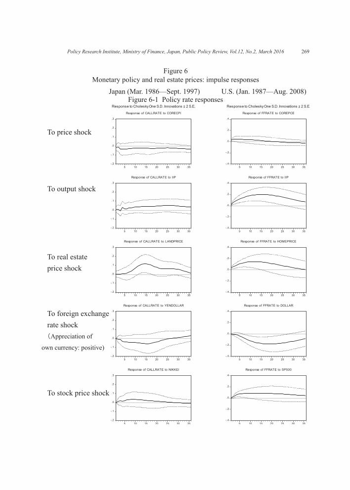
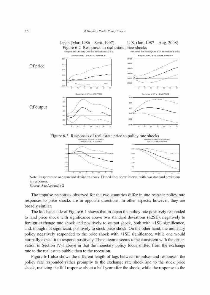
To consider these questions, we estimated vector auto-regression (VAR) models with six variables (general price, industrial production, real estate price, policy rate, exchange rate and stock price) for Japan and the U.S. Figure 6-1 shows policy rate responses to shocks in other variables, Figure 6-2 price and output responses to real estate price shocks, and Figure 6-3 real estate price responses to policy rate shocks. Japanese results are shown on the right-hand side and those of the U.S. on the left. See Appendix 2 for data used.


269

Figure 6Monetary policy and real estate prices: impulse responses

U.S. (Jan. 1987—Aug. 2008)Japan (Mar. 1986—Sept. 1997)Figure 6-1 Policy rate responses


The impulse responses observed for the two countries differ in one respect: policy rate responses to price shocks are in opposite directions. In other aspects, however, they are broadly similar.

The left-hand side of Figure 6-1 shows that in Japan the policy rate positively responded to land price shock with significance above two standard deviations (±2SE), negatively to foreign exchange rate shock and positively to output shock, both with ±1SE significance, and, though not significant, positively to stock price shock. On the other hand, the monetary policy negatively responded to the price shock with ±1SE significance, while one would normally expect it to respond positively. The outcome seems to be consistent with the obser-vation in Section IV-1 above in that the monetary policy focus shifted from the exchange rate to the real estate bubble then to the recession.

Figure 6-1 also shows the different length of lags between impulses and responses: the policy rate responded rather promptly to the exchange rate shock and to the stock price shock, realizing the full response about a half year after the shock, while the response to the

Note: Responses to one standard deviation shock. Dotted lines show interval with two standard deviations in responses.Source: See Appendix 2

Figure 6-3 Responses of real estate price to policy rate shocks

Figure 6-2 Responses to real estate price shocksU.S. (Jan. 1987—Aug. 2008)Japan (Mar. 1986—Sept. 1997)


271

real estate price shock was slower, reaching full response more than a year after the shock. The difference is consistent with the difference in the timely availability of statistical data.

The right-hand side of Figure 6-1, which shows the U.S. results, gives a largely similar picture. In the U.S., the policy rate responded positively to the real estate price shock, nega-tively to the foreign exchange shock and positively to the output shock, all with ±3SE sig-nificance, and positively to the stock price shock with ±2SE significance. Unlike the out-come for Japan, the response to the price shock was consistent with the direction one would expect: the policy rate responded to price shock positively with ±2SE significance.

U.S. monetary policy did respond to price and output, but also to house price, stock price and foreign exchange rate shocks.

The outcome is consistent with some of the remarks of Federal Reserve leadership. In-deed, Greenspan (2007) admits that the Fed intended to respond to stock market and house price shocks. He says that the tightening in 2004 was done “to raise mortgage rates to levels that would defuse the boom in housing, which by then was producing an unwelcome froth.” He also says that in making the March 1997 tightening “the FOMC statements . . . did not say a word about asset values or stocks” since “if we . . . gave as a reason that we wanted to rein in the stock market, it would have provoked a political firestorm,” and the series of rate cuts in 2001 was “to mitigate the impact of the dot-com bust and the general stock-market decline.”

The response to foreign exchange shock is admitted more openly: The Fed Board web-site explains that “movements in the exchange value of the dollar represent an important consideration for monetary policy—such movements exert influence on U.S. economic ac-tivity and prices and constitute one of the ways the effects of monetary policy reach the broader economy.”6

The Figure also indicates that U.S. monetary policy responded fully to stock price and price shocks within a few months but took around one year until it fully responded to the real estate price, output and foreign exchange shocks.

Figure 6-2 shows that in both countries the price responded to the real estate price shock with a two year lag and the output with a one year lag.

Figure 6-3 shows that in both countries the real estate price responded to the policy rate shock with a lag longer than two years.

The Japanese and the U.S. experience may be interpreted as follows:- The Bank of Japan and the Federal Reserve reacted to real estate prices perhaps partly

to contain the bubbles and partly to preempt future impact on output and inflation.- Monetary policy reaction to real estate price move took about a year, but the effects of

real estate price move on price and output fully materialized together one year later.7

- As a result their policy rates moved in timely way with the contemporaneous inflation and output and in line with the Taylor rule.

6 http://www.federalreserve.gov/faqs/economy_12763.htm, accessed in May 2015.7 Increased consumption due to the asset effect, increased borrowing and investment due to collateral value increase and infla-tion due to house rent increase all happen with lags.


- There also was a two-year lag between a policy action and its effects on real estate prices.

The above sequence means that a real estate price peak out in Year 0 results in a mone-tary policy turn-around in Year 1 (as we saw in Figure 4) and its effects on real estate price fully materialize in Year 3. Therefore, timely policy action tuned to inflation and output can exacerbate the collapse of the bubbles and can work to amplify the real estate cycle.

IV-3. Implications on the clean versus lean debate

What does the monetary policy experience in both countries imply with regard to the clean versus lean debate?

First, the characterization of historical episodes in the clean versus lean debate we saw in Section II may not necessarily be consistent with what happened. The clean school criti-cized the Japanese monetary policy in 1989 and 1990 for intentionally trying to prick the bubble, but it was no tighter than the Taylor target. The size of the tightening was similar to that in the U.S. in 2005 and 2006. The Federal Reserve advocated the importance of easing to mitigate the impact of the bubble burst, but its clean-up operation was no more aggressive than the Bank of Japan or than the Taylor target in its timing and depth of cuts.

Second, though both the clean and lean views seem to focus on how far the monetary policy is additionally tightened or eased by taking asset prices and credit expansion into consideration, the real life relationship among asset prices, inflation and output, and policy stance seems to include many complicated interactions, resulting from lags in recognition, action and effect.

Orphanides (2003) shows that a monetary policy following the Taylor rule does not per-form well if data available to policymakers in real time is used instead of the final data, which is not available in real time. The policy authorities in real life, however, do not me-chanically respond to the available inflation and output statistics, which are backward look-ing, but modify them to form a forward looking view by incorporating data on asset prices, foreign exchange rates and commodity prices and qualitative information derived from in-terviews. But even if such modification is successful, the lags between asset price and its ef-fects on inflation and output, and between monetary policy action and its effects on real es-tate price may allow timely policy action to destabilize the system.

V. Prudential policy

V-1. Japan’s experience

The Ministry of Finance, which then was the bank regulator, implemented from 1986 to 1989 a series of qualitative administrative guidances, gradually intensifying the measures taken (Figure 7). In ordinary cases, guidances weaker than these often have significant ef-fects. For example, the Financial Services Agency in December 2006 added in its annual su-


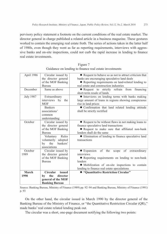
273

pervisory policy statement a footnote on the current conditions of the real estate market. The director general in charge published a related article in a business magazine. These gestures worked to contain the emerging real estate froth. The series of actions taken in the latter half of 1980s, even though they went as far as reporting requirements, interviews with aggres-sive banks and on-site inspections, could not curb the rapid increase in lending to finance real estate investments.

Source: Banking Bureau, Ministry of Finance (1989) pp. 92–94 and Banking Bureau, Ministry of Finance (1991) p. 93

Figure 7Guidance on lending to finance real estate investments

On the other hand, the circular issued in March 1990 by the director general of the Banking Bureau of the Ministry of Finance, or “the Quantitative Restriction Circular (QR),” made banks’ real estate related lending peak out.

The circular was a short, one-page document notifying the following two points:


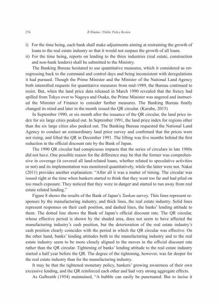
i) For the time being, each bank shall make adjustments aiming at restraining the growth of loans to the real estate industry so that it would not surpass the growth of all loans.

ii) For the time being, reports on lending to the three industries (real estate, construction and non-bank lenders) shall be submitted to the Ministry.The Banking Bureau hesitated to use quantitative measures, which it considered as ret-

rogressing back to the command and control days and being inconsistent with deregulations it had pursued. Though the Prime Minister and the Minister of the National Land Agency both intensified requests for quantitative measures from mid-1989, the Bureau continued to resist. But, when the land price data released in March 1990 revealed that the frenzy had spilled from Tokyo over to Nagoya and Osaka, the Prime Minister was angered and instruct-ed the Minister of Finance to consider further measures. The Banking Bureau finally changed its mind and later in the month issued the QR circular. (Karube, 2015)

In September 1990, or six month after the issuance of the QR circular, the land price in-dex for six large cities peaked out. In September 1991, the land price index for regions other than the six large cities also peaked out. The Banking Bureau requested the National Land Agency to conduct an extraordinary land price survey and confirmed that the prices were not rising, and lifted the QR in December 1991. The lifting was five months behind the first reduction in the official discount rate by the Bank of Japan.

The 1990 QR circular had conspicuous impacts that the series of circulars in late 1980s did not have. One possible reason for the difference may be that the former was comprehen-sive in coverage (it covered all land-related loans, whether related to speculative activities or not) and its implementation was monitored quantitatively, while the latter were not. Nakai (2011) provides another explanation: “After all it was a matter of timing. The circular was issued right at the time when bankers started to think that they went too far and had piled on too much exposure. They noticed that they were in danger and started to run away from real estate related lending.”

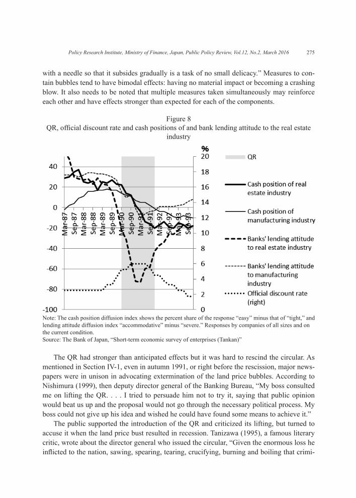
Figure 8 shows the results of the Bank of Japan’s Tankan survey. Thin lines represent re-sponses by the manufacturing industry, and thick lines, the real estate industry. Solid lines represent responses on their cash position, and dashed lines, the banks’ lending attitude to them. The dotted line shows the Bank of Japan’s official discount rate. The QR circular, whose effective period is shown by the shaded area, does not seem to have affected the manufacturing industry’s cash position, but the deterioration of the real estate industry’s cash position clearly coincides with the period in which the QR circular was effective. On the other hand, banks’ lending attitudes both to the manufacturing industry and to the real estate industry seem to be more closely aligned to the moves in the official discount rate rather than the QR circular. Tightening of banks’ lending attitude to the real estate industry started a half year before the QR. The degree of the tightening, however, was far deeper for the real estate industry than for the manufacturing industry.

It may be that the tightened monetary policy, bankers’ growing awareness of their own excessive lending, and the QR reinforced each other and had very strong aggregate effects.

As Galbraith (1954) maintained, “A bubble can easily be punctuated. But to incise it


275

with a needle so that it subsides gradually is a task of no small delicacy.” Measures to con-tain bubbles tend to have bimodal effects: having no material impact or becoming a crashing blow. It also needs to be noted that multiple measures taken simultaneously may reinforce each other and have effects stronger than expected for each of the components.

Note: The cash position diffusion index shows the percent share of the response “easy” minus that of “tight,” and lending attitude diffusion index “accommodative” minus “severe.” Responses by companies of all sizes and on the current condition.Source: The Bank of Japan, “Short-term economic survey of enterprises (Tankan)”

Figure 8QR, official discount rate and cash positions of and bank lending attitude to the real estate

industry

The QR had stronger than anticipated effects but it was hard to rescind the circular. As mentioned in Section IV-1, even in autumn 1991, or right before the rescission, major news-papers were in unison in advocating extermination of the land price bubbles. According to Nishimura (1999), then deputy director general of the Banking Bureau, “My boss consulted me on lifting the QR. . . . I tried to persuade him not to try it, saying that public opinion would beat us up and the proposal would not go through the necessary political process. My boss could not give up his idea and wished he could have found some means to achieve it.”

The public supported the introduction of the QR and criticized its lifting, but turned to accuse it when the land price bust resulted in recession. Tanizawa (1995), a famous literary critic, wrote about the director general who issued the circular, “Given the enormous loss he inflicted to the nation, sawing, spearing, tearing, crucifying, burning and boiling that crimi-


nal would not be enough.” Apparently Tanizawa was not aware that it was the director gen-eral who most strongly resisted the political pressures demanding the QR. A popular science fiction movie “Bubble Fiction: Boom or Bust” released in 2007 depicted a heroine who used a time machine to go back to 1990 and fought with the wicked director general to block the QR. The heroine returned to 2007 Japan and found the country in glittering prosperity after two decades of continued boom.

The experience seems to show that a prudential policy tool can have wide ramifications on the economy. Indeed, Sonoda and Sudo (2015) compare the effects that monetary and prudential policy measures had on macro-economy and asset prices from 1970 to 2000 by constructing a Factor-Augmented VAR model and find that both the QR and the monetary policy had sweeping effects on the output and its components. This finding casts doubt on the clean thesis that prudential policy measures can have focused effects while monetary policy measures are more broad brushed.

It is not simple to find what we should have done, but we may want to think of the fol-lowing three alternatives.

First, it may have been better to start and end the QR earlier. Earlier, Japan had another QR episode, in which QR was introduced in an earlier phase of the bubble, lasted for a shorter period, and seems to have been more successful than the 1990 one. In January 1973, the Ministry of Finance issued a circular to contain lending related to the acquisition of land, which resembled the 1990–1991 QR,8 and kept it for a year until December. (Banking Bu-reau, Ministry of Finance, 1973)

The 1970 QR also had a strong impact. The quarter-on-quarter growth rate of loans to the real estate industry dropped from 15.5% in 4Q 1972 to 4.7% in 2Q 1973. The growth rate of the land price index for the six large city areas over the previous half-year period also dropped from 15.4% in the half year ending March 1993 to －7.8% in the half year ending March 1975. Nevertheless, the nominal real estate price turned stable in the half year ending September 1975 and no protracted decline ensued. The impact on the financial system was also limited.

The hyper-inflation in the wake of the 1973 oil crisis contributed to mask the real estate shock as it supported the nominal land price. The timing, however, may have also mattered. The 1972 QR was introduced promptly, or less than a year after the start of the land boom, while the 1990 QR was introduced four years after the start of the boom. In addition, the 1973 QR lasted only for a year, while the one in 1990 lasted for two years. The prompt in-troduction may have limited the total size of the bubble and thus that of the burst, and the shorter duration may have limited the impact of the regulation.

Second, it may have been better to find measures more articulate than moral suasions but less brutal than the QR. However, compared to those dealing with housing booms, mac-ro-prudential tools on commercial real estate (CRE) booms are less well explored and ex-

8 The circular imposed the target of “limiting the growth of land-acquisition related lending to the growth of total lending” and requested that banks submit quarterly plans and results to the Ministry of Finance.


277

perimented on. In its macro-prudential policy toolkit, IMF (2014) lists, in addition to caps on CRE exposures, measures such as higher Basel III risk weights on total or new CRE loans, loan-to-value (LTV) ratio limits, debt-service-coverage (DSC) ratio limits and combi-nations thereof (for example, higher risk weights on high loan-to-value loans). But measures on banks tend to be circumvented and boost shadow banking particularly when applied to corporate loans, whose large lots can justify the cost needed to craft circumvention schemes. Japan’s QR is said to have helped Jusen non-bank lenders to swell in the early 1990s and complicated clean-up operations afterwards. In addition, when real estate value is rising, loan-to-value ratio tends to decline and limits on them may become less binding. Ono et. al. (2014), using a dataset compiled from Japan’s official real estate registry from 1975 to 2009, find that LTV ratios were at their lowest during the real estate booms in the late 1980s and early 1990s. One promising candidate may be the use of stress tests focusing on real estate prices.

Third, what lacked then may have been not macro-prudential measures to cap aggregate lending but micro-prudential measures to make bankers assess the viability of borrowers’ projects more accurately and prudently. Yoshikawa (1999) argues that the biggest problem of the policy taken during the boom was that it aimed at the containment of the land price boom and not the soundness of bank lending or banks’ risk management practices. Sound banking, or skills to tell good projects from bad ones and a discipline to lend only for the former, indeed is the strongest bulwark against an irrational exuberance.

The two illusions which fueled the bubble, or the belief that Tokyo was becoming a global financial center ranking with New York and London and that the Japanese people, with more money and holidays than before, would need more luxurious resorts across the country, were widely shared among the government, bankers and borrowers. The illusion would have biased the assessments of the viability of projects anyway. But a more rigorous assessment of future cash flow should have weeded at least the most speculative of the proj-ects at the time, which later turned pure bad loans.

IV-2. Comparison with the U.S. experience

Just like their Japanese counterparts, the US authorities started to issue qualitative guid-ance from a very early stage in the real estate price bubble and continued to add new mea-sures for several years. Though the Japanese ones were mainly preaching of business ethics and the U.S. ones were micro-prudential, both were qualitative and were not effective enough to contain imprudent lending. Only after the initial signs of the busts (the stock price peak-out in the case of Japan, and the house price peak-out in the case of the US), both im-posed quantitative guidance with specific numerical criteria, terminating the booms and deepening the busts.

The US agencies (the Federal Reserve, the OCC and the FDIC) jointly issued a series of guidance on real estate related loans from 1999, as listed in Figure 9. Most of them were qualitative, but the Interagency Guidance on Concentration in Commercial Real Estate


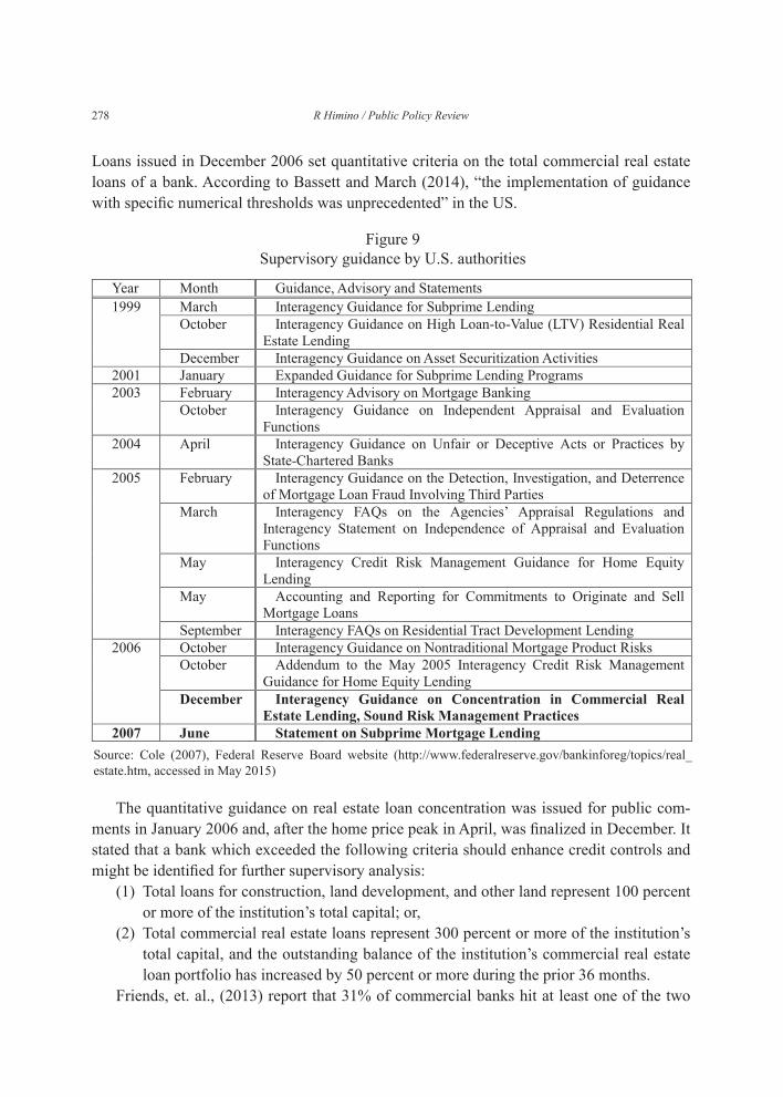
Loans issued in December 2006 set quantitative criteria on the total commercial real estate loans of a bank. According to Bassett and March (2014), “the implementation of guidance with specific numerical thresholds was unprecedented” in the US.

Source: Cole (2007), Federal Reserve Board website (http://www.federalreserve.gov/bankinforeg/topics/real_ estate.htm, accessed in May 2015)

Figure 9Supervisory guidance by U.S. authorities

The quantitative guidance on real estate loan concentration was issued for public com-ments in January 2006 and, after the home price peak in April, was finalized in December. It stated that a bank which exceeded the following criteria should enhance credit controls and might be identified for further supervisory analysis:

(1) Total loans for construction, land development, and other land represent 100 percent or more of the institution’s total capital; or,

(2) Total commercial real estate loans represent 300 percent or more of the institution’s total capital, and the outstanding balance of the institution’s commercial real estate loan portfolio has increased by 50 percent or more during the prior 36 months.

Friends, et. al., (2013) report that 31% of commercial banks hit at least one of the two


279

thresholds and they held almost 40% of all outstanding commercial real estate loans. Though the guidance stated that the criteria did not constitute limits on lending activities, bankers feared that individual examiners would enforce it as limits (Bassett and March, 2014). The guidance was clearly effective: Construction and development loans, which grew at an annualized rate of around 30% before the issuance for public comments, increased only at around 10% after the finalization of the guidance, and started to decline one year af-ter (ibid). About a half year after the finalization, commercial real estate prices peaked out.9 It may be recalled that in Japan, as well, the six large city land price index peaked out a half year after the issuance of the QR guidance.

Bassett and March (2014) say, “[T]he implementation of the guidance coincided with the early stages of the economic downturn that culminated with the financial crisis. As such, the intended effect of the guidance—preventing further buildups of concentrated real estate exposures—may have helped some banks avoid even worse outcomes in the subsequent real estate crash. However . . . the guidance may have had the unintended effect of exacerbating the downturn, particularly in some local markets served by banks that had chosen to special-ize in commercial real estate loans.” The comments remind us of the role the QR circular played in Japan. In the previous section we saw some similarities between the conduct of monetary policy in Japan and the US, but it seems that the conduct of prudential policy in the two countries also resembled each other.

With regard to subprime mortgage lending, which was the chief cause of the US boom and bust, five federal agencies (the OCC, the FRB, the FDIC, the OTS and the NCUA) is-sued a statement for public comments in March 2007 and finalized it in June. Though it was one year after the home price peak and the mortgage delinquency and foreclosure rates were already on the rise, it just confirmed the principle, which might go without saying and had already been confirmed by the October 2006 guidance, that a banker should evaluate the borrower’s ability to repay the debt at the fully indexed rate (i.e., not at the low “teaser” rate for the first two or three years but at the rate effective for the remaining 28 or 27 years) and assuming a fully amortizing repayment schedule (even in the case of the “negative amorti-zation” products, which allow shortfall on the interest payment to be added to the principle).

Nevertheless, soon after the issuance of the draft statement for public comments, repre-sentatives of the OCC, the FRB, the FDIC, the OTS and the Conference of State Bank Su-pervisors10 were requested to testify at a congressional hearing and had no choice other than to unanimously vow never to limit the availability of credit. It seems that the political diffi-culty in dealing with residential mortgage was by far greater than the one related to com-mercial mortgages.

9 The Costar Commercial Repeat Sales Indices (U.S. Composite) peaked in August 2007 (Equal Weighted series) or in Sep-tember 2007 (Value Weighted series). The Green Street Commercial Property Price Index peaked in August 2007. Moody’s/RCA US Indices peaked either in the third or fourth quarter of the year.10 The Conference of State Bank Supervisors earlier had issued a press release indicating their intent to develop a statement parallel to the federal one.


VI. Tax, land and fiscal policies

In addition to monetary and prudential policies, tax and land policies were mobilized to contain the real estate boom in Japan. Fiscal policy was deployed to mitigate the depression in the wake of the collapse of the bubble.

Starting with the tax law amendments in September 1987, a series of measures were tak-en to tighten taxation on land capital gains and on the holding of land. Some of the measures were implemented with significant delay and should have worked to accelerate the land price declines. For example, the Land-Holding Tax was implemented with the rate of 0.2% from January 1992, when the land prices were declining nationwide, and 0.3% from 1993. It was maintained throughout the land price free fall until 1997, when the six-city area land price went down as far as to one quarter of the peak level. Another example was the ap-praised land prices for local tax on real estate holding, which was raised dramatically in fis-cal year 1993.

With regard to the land policy, the National Land Utilization Law was amended in June 1987 to introduce a system of land price monitoring zones. Local governments were given the power to designate monitoring zones, advise suspension or alteration of particularly in-appropriate transactions, and publish the names of those who did not abide by the advice. The power, however, was rarely activated, as it was difficult to determine that a specific transaction was inappropriate.

The land policy’s new objective, namely “crash the land myth” (which meant ending the widely-held belief that land prices never fall), was announced as late as in January 1991, when land prices for the six large city areas had already peaked out, and was maintained all through the land price free-falls, with various new measures added to increase the supply of land. For example, in 1992, when land prices were falling across the country, it was made easier to transfer land from agricultural use to residential use. In the same year, new forms of land lease contracts were introduced to provide more flexibility in the land-supply modal-ity. The “crash the land myth” banner was replaced with “enhance liquidity in the real estate market” only in 1997.

Fiscal policy was mobilized to mitigate the recession in the wake of the collapse of the bubble. In March 1992, the government published a stimulus package and announced that the implementation of the public works budgeted for fiscal year 1992 would be front loaded. In August 1992, an additional stimulation package with a total expenditure amounting to 10.7 trillion yen was announced. Further stimulation packages ensued.

VII. Assessing Japan’s responses

Earlier in Section I we asked the question whether the timing, calibration, and choice of tools were appropriate or not. Even in hindsight, the review above could not conclude on the choice of tools: we could not be confident whether monetary policy or prudential policy


281

would have been better suited to the need. With regard to calibration, the 1986 easing may have been less aggressive than ideal and the 1990 combination of the monetary policy tight-ening and the QR may have been too aggressive in aggregate.

We had somewhat clearer conclusions on timing: there seem to have been several key delays. For example, monetary easing and major fiscal stimulus were added in 1987, when the economy was recovering and the rapid land price hike started. Monetary tightening start-ed only in 1989. The QR were introduced and the official discount rate was raised to 6% in 1990, when the stock price was plummeting and the six large city area land price peaked out. The QR was rescinded and the official discount rate was reduced only in late 1991.

The policy responses in Japan were broadly synchronized with the shifts in national pri-ority from yen to land and from land to recession, and were delayed one to two years from the developments in bubbles and busts.

The following three reasons may explain the delay.First, other policy priorities may have prevented timely responses.The measures to contain bubbles were delayed as they were thought to be in conflict

with the need to address the strong yen. The change in policy direction from containment of bubbles to the mitigation of their collapse was delayed as it was thought to go against the aim of containing land price bubbles and of restoring fair distribution of wealth. On the oth-er hand, no one had foreseen the deep impact of the collapse of the bubbles, and the minimi-zation of the impact could not have been a policy priority of the time.

When discussing responses to bubbles, one tends to focus on the period around the bub-ble peak, but during that period, policy latitude may be significantly constrained due to other policy priorities. Extreme swings can trigger an allergy in public opinion (e.g., on yen or on land price) and constrain timely policy change in the ensuing periods. To be effective, we need to moderate the swing throughout the credit cycle: a 1986 easing may have been more important than a 1987 tightening.

Second, recognition lag may explain part of the delay.The land price indices during the period under study were published infrequently and

with significant delays. Significant time was needed to confirm that the land prices had peaked out. The Urban Land Price Index by the Japan Real Estate Institute has been pub-lished semiannually and with a two-month lag. One could have noticed the start of a slight decline in six city area land price only eight months after the peak and could have confirmed a clear sign of decline only one year and two months after. If one used the Land Price Public Notice (January price with two month delay) and the Market Values of Standard Sites (July price with two month delay) both published by the National Land Agency, a similar recogni-tion should have required four to six more months.

On the other hand, the recognition lag should have been much shorter in the U.S. in the 2000s. The Case-Shiller home price index and the Office of Federal Housing Enterprise Oversight home price index were published monthly with a two month delay, and the First American Core Logic house price index monthly with a five week delay. In making timely policy decisions, the Japanese authorities in the 1990s were far more disadvantaged than


their U.S. counterparts in the 2000s.Today, more timely information is available in Japan than in the 1990s, including the

Recruit Residential Price Index (monthly with one month delay), the Tokyo Stock Exchange Home Price Index (monthly with two month delay), the Japan Residential Property Price In-dex (monthly with four month delay) and the Trend Report of the Values of Intensively Used Land in Major Cities (quarterly).

The recognition lag is also significant with regard to the peaks and troughs in business cycles. Seven months after the February 1991 peak, the government’s monthly economic re-port modified its view from “in an expansion trend” to “still expanding with gradual decel-eration” and after 11 months to “in an adjustment process”. There are often several percent-age points of difference among the first quick estimate of the GDP growth rate, the second quick estimate and the final estimate. The final estimate is published nine to 18 months after the end of the estimated quarter.

One cannot shorten the lag between actions and effects but can shorten the recognition and reaction lags. Improvements in frequency, promptness and accuracy of statistical publi-cations will help reduce recognition lags and may make policy responses timelier.

Third, the tax and land policy measures to reduce land prices were kept long after the collapse of the bubbles, perhaps because their objectives differ from those of macro-eco-nomic or prudential policies.

The changes in land prices matter more than the level for financial stability, but the lev-els matter more for taxation purposes, since declining but high land prices still indicate land holders’ capability to bear the tax burden. The levels matter also for land policy, which aims to make it possible for people to use land at reasonable prices.

VIII. Conclusion

Assertions made in the clean versus lean debate have not necessarily been consistent with what we found in the two episodes reviewed in this paper. The U.S. Federal Reserve denounced what the Bank of Japan did in the 1990s, but U.S. policy rates moved almost in parallel with the Japanese ones during the six year window around the real estate price peak. Though the Bank of Japan is believed to have intentionally pricked the bubble, their tighten-ing did not exceed the Taylor target. The easing by the Federal Reserve, in spite of its advo-cacy of ex-post clean-up operation, did not exceed the Taylor target either.

In addition, the behavior of the prudential authorities of the two countries resembled each other in that they implemented qualitative measures from the very early stages of the bubbles, continued to add layers of qualitative measures over several years and finally took the step of implementing quantitative measures at the last stage of the bubble, ending the boom and exacerbating the bust.

In reality, intention, action and effects were staggered with each other. Monetary policy which may have been “clean” in its intention worked as a belated “lean.” The U.S. quantita-tive guidance on commercial real estate lending in 2006 listed micro-prudential purposes


283

(sound risk management practices and proper evaluation of capital adequacy), but had a macro-prudential effect of killing the boom and deepening the bust.

The review, by focusing on the real estate price moves as a benchmark, found several delays in the timing of policy changes both in Japan and in the U.S. It seems that the timing of policy measures matters more than how they are motivated, explained, or labelled; clean or lean, micro- or macro-prudential.

The following points may be useful in trying to improve the timeliness of policy re-sponses.i) Prices of different asset classes peak out not simultaneously but in intervals, and the se-

quences may differ among episodes. Thus, we should not presume specific sequences and predetermine which index is a leading indicator. Ascertaining a turning point is not easy, but more frequent publication of more accurate economic statistics with smaller delay would help enable timely policy actions.

ii) Optimum policy to minimize the impacts of bubbles can conflict with other high priority policy objectives at the time. To secure necessary wriggle room in critical phases, policy authorities should try to limit the swing throughout a credit cycle. Earlier stages do mat-ter.

iii) Policy choices have to be made under pressure from public opinion and the political sector. Japan’s experience shows that pressure can be in both directions, tightening and easing, and that experts made better judgments in some cases but, in other cases, those who exerted pressure on experts had better insights. Policy authorities therefore should try to engage constructively with political and public pressures, not taking the matter as a game of giving-in or not. Wide consensus on the dynamics of bubbles and on the ef-fects of policy measures would help attain constructive engagements.

Appendix 1: Data used for Figure 5: Actual policy rates and Taylor target

Actual policy rates

The Bank of Japan’s target rate has been the uncollateralized overnight call rate (shown by the thick solid black line in the figure) since 1998. The official discount rate (thick solid grey line) represented the monetary policy stance until 1998. The figure shows both rates. For the U.S., the Federal Fund rate is shown (thick solid line).

Inputs used to calculate the Taylor targets

In calculating the Taylor targets, we used the price level indices on which the central bank in question is said to focus. For Japan, we used the Consumer Price Index excluding fresh food and adjusted it for the effects of the changes in VAT. As the Ministry of Internal Affairs and Communication publishes the seasonally adjusted series only for the period starting in 2000, we made seasonal adjustment to the original series from 1980 to 1Q 2014


using the Census X-13. For the U.S., we used the seasonally adjusted series of the personal consumption expenditure deflator excluding food and energy.

Bernanke and Gertler (1999) use the inflation-expectation targeting rule, which assumes that the central bank foresees the inflation rate of one year ahead, while Judd and Rudebusch (1998) use the inertial interest-rate dynamics, which assumes that the central bank responds gradually to changes in the environment. We used the contemporaneous response rule which Taylor (1993) adopted, as our purpose is to compare the timeliness of central banks’ re-sponses.

Though Taylor (1993) used the change rate of price index over a year ago as the inflation rate, we used annualized change rate over the previous quarter, as the former’s move tends to lag behind the latter’s and the latter would form a more demanding benchmark in measur-ing the timeliness in the response. The result seems to imply that the actual policy rate moved in line with the contemporaneous response using the annualized change rate over the previous quarter.

The GDP gap is the ratio of the difference between the actual GDP level and the poten-tial GDP level relative to the potential GDP level. There are various ways to estimate the potential GDP level. Though Taylor (1993) assumed that the potential growth rate was 2.2% for the five year period he studied, a single potential growth rate over a 10 year window we examine would be less plausible.

We used the approach for Japan and the U.S. of applying the Hodrick–Prescott filter with a smoothing factor of 1600 to the quarterly seasonally adjusted real GDP level data from 1Q 1980 to 1Q 2014 (the Taylor target derived by this approach is indicated by thin dashed line).

We also used the GDP gap estimated by the Cabinet Office (thin solid line) and the Bank of Japan (thin chain line) for Japan and the one by the Congressional Budget Office (thin solid line) for the U.S.

There is a large gap between the HP filter estimates and the CBO estimates for the peri-od after 2009 in the U.S., but the difference due to GDP gap estimation approaches is not significant for the rest.

Response coefficients

Whereas Figure 5 uses 0.5 as the response coefficient to the GDP gap as proposed by Taylor (1993), Taylor (1999) proposes an alternate coefficient of 1, doubling monetary poli-cy response to the GDP gap. The following figures show the target rates derived by applying the Taylor (1999) proposal. The overall findings from Figure 5 seem to apply to the Taylor (1999) based figures, but the following difference may be noticed: a) The gap between the actuals and the targets are bigger both for Japan and the U.S., particularly during the period after the policy rates hit the zero lower bound; b) the Taylor (1999) target suggests more ag-gressive tightening and easing for Japan; and, c) the U.S. delay in tightening starts from the latter half of 2003, rather than in the first half of the year.


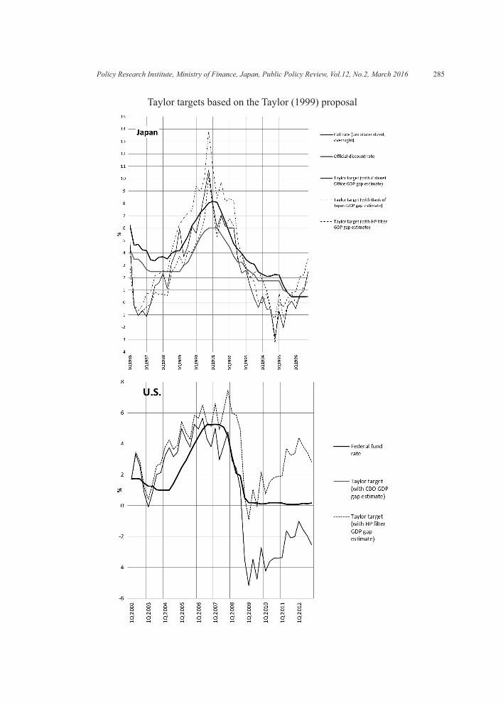
285

Taylor targets based on the Taylor (1999) proposal


Appendix 2: The VAR model used for Figure 6

Japan

The sample period is set between March 1986, when the land price bubble started to emerge, and October 1997, one month before the outbreak of the systemic banking crisis.

Three non-financial variables (consumer price index excluding fresh food, industrial production index and commercial land price index for the six large city area), one policy variable (uncollateralized overnight call rate) and two financial variables (yen-dollar ex-change rate and Nikkei 225 stock price index) are included as they play key roles in the de-scription of the developments in Japan in Sections III.

We interpolated the land price index, which is available only semiannually, by cubic spline. We applied Census X13 seasonal adjustment to the CPI series after adjusting for the impact of the changes in VAT. Other variables are not seasonally adjusted.

We used a logarithm of level variables. The variables are likely to have unit roots but we used levels rather than differences following Sims, Stock and Watson (1990). Guided by Christiano, Eichenbaum and Evans (1999), we put non-financial variables first followed by a policy variable and then by financial variables in making the Cholesky decomposition.

We set the lag order at four using the Akaike Information Criterion (AIC).The outcome was broadly similar when we used official discount rate instead of call rate

or the effective real exchange rate instead of the yen-dollar exchange rate. Alternative order of variables in the Cholesky decomposition (making the land price first, call rate first, or ex-change rate first) did not alter the outcome significantly.

Earlier start of the sample period (adding the period from December 1980, when the control on foreign exchange transaction was lifted) made the response of policy rate to land price shock smaller and that to foreign exchange rate shock larger. On the other hand, the later end of the sample period (adding the period until March 2001, when the quantitative easing policy was adopted) made the response of policy rate to land price shock larger and that to foreign exchange rate shock smaller.

The VAR model does not consider the effects of tax policy, land policy, fiscal policy, foreign exchange intervention, quantitative restrictions, or the Bank of Japan’s window guidance. Not enough land-price samples were used as we interpolated semiannual data. In-terest rate deregulation, which was started in 1985 and completed in 1994, should have changed the model structure but we assumed constant parameters for the entire sample peri-od. These points constrain the robustness of the outcome.

U.S.

The sample period is set between January 1987, when the Case-Shiller 10 city home price index becomes available and August 2008, one month before the collapse of Lehman


287

Brothers. The policy rate hit the zero lower bound four months after the end of the sample period.

Three non-financial variables (personal consumption expenditure deflator excluding food and energy, industrial production index and Case-Shiller 10 city home price index), one policy variable (Federal Fund rate) and two financial variables (trade weighted real ex-change rate and S&P 500 stock price index) are included. We used a seasonally adjusted se-ries for the PCE deflator, industrial production index and home price index. We used a loga-rithm of level variables. We used levels rather than differences. We ordered variables as shown above in making the Cholesky decomposition.

We set the lag order at three using the AIC.Changing the lag order from three to four did not significantly alter the outcome. An al-

ternative order of variables in the Cholesky decomposition (making the home price first, policy rate first, or exchange rate first) did not alter the outcome significantly, either.

References

Ahearne, A., J. Gagnon, J. Haltmaier and S. Kamin (2002), “Preventing Deflation: Lessons from Japan’s Experience in the 1990s”, International Finance Discussion Papers, Number 729, Board of Governors of the Federal Reserve System

Banking Bureau, Ministry of Finance (1973), The 22nd Annual Report of the Banking Bu-reau, 1973 edition (Dai 22-kai Ginkou-kyoku Kinyuu Nenpou, Shouwa 48-nen ban), Kinzai Institute for Financial Affairs, Inc.

_____ (1989), The 37th Annual Report of the Banking Bureau, 1988 edition (Dai 37-kai Ginkou-kyoku Kinyuu Nenpou, Shouwa 63-nen ban), Kinzai Institute for Financial Af-fairs, Inc.

_____ (1989), The 39th Annual Report of the Banking Bureau, 1990 edition (Dai 39-kai Ginkou-kyoku Kinyuu Nenpou, Heisei 2-nen ban), Kinzai Institute for Financial Af-fairs, Inc.

Bernanke, B. (2002), “On Milton Friedman’s Ninetieth Birthday”, Remarks at the Confer-ence to Honor Milton Friedman, University of Chicago, Chicago, Illinois, Board of Governors of Federal Reserve System

Bernanke, B. and M. Gertler (1999), “Monetary Policy and Asset Price Volatility”, in Feder-al Reserve Bank of Kansas City, New Challenges for Monetary Policy

Borio, C. (2014), “Monetary policy and financial stability: what role in prevention and re-covery?”, BIS Working Papers, No.440, Bank for International Settlements

Borio, C. and W. White (2004), “Whither monetary and financial stability? The implications of evolving policy regimes”, BIS Working Papers No 147, Monetary and Economic Department, Bank for International Settlements

Christiano, L., M. Eichenbaum and L. Evans (1999), “Monetary Policy Shocks: What Have We Learned and to What End?” in J. Taylor and M. Woodford, eds., Handbook of Mac-roeconomics 3A, Elsevier Science B.V., pp. 65–148


Del Negro, M. and C. Otrok (2007), “99 Luftballons: Monetary policy and the house price boom across U.S. states”, Journal of Monetary Economics, 54 (7). pp. 1962–1985

Federal Reserve Bank of Kansas City (2003), Monetary Policy and Uncertainty: Adapting to a Changing Economy

Fisher, S. (2014), “Macroprudential Policy in Action”, in G. Akerlof, O. Blanchard, D. Romer and J. Stiglitz eds., What Have We Learned? Macroeconomic Policy after the Crisis, The MIT Press

Friedman, M. and A. Schwartz (1963), A Monetary History of the United States, 1867–1960, NBER and Princeton University Press

Galbraith, J. (1954), The Great Crash 1929, Penguin BooksGlaeser, E., J. Gottlieb and J. Gyouriko (2010), “Can cheap credit explain the housing

boom?”, NBER working paper series 16230, National Bureau of Economic ResearchGreenspan, A. (2007), The Age of Turbulence, Adventures in a New World, The Penguin

PressHamada, K., A. Kashyap and D. Weinstein (2011), “Introduction”, in K. Hamada, A. Kashy-

ap and D. Weinstein, eds., Japan’s Bubble, Deflation, and Long-term Stagnation, The MIT Press

IMF (2011), “Box 1.4. Did the Plaza Accord Cause Japan’s Lost Decades?”, in World Eco-nomic Outlook, April, International Monetary Fund

_____ (2014), “Staff guidance note on macroprudential policy: Detailed guidance on instru-ments”, International Monetary Fund

Jarocinski, M. and F. Smets (2008), “House Prices and the Stance of Monetary Policy”, Federal Reserve Bank of St. Louis Review, 90, pp. 339–365

Jinushi, Y, Y. Kuroki and R. Miyao (2000), “Monetary Policy in Japan since the late 1980s: Delayed policy Actions and Some Explanations”, in R. Mikitani and A. Posen ed. Ja-pan’ s Financial Crisis and Its Parallels to U.S. Experience, Institute of International Economics, Special Report 13

Judd, J. and G. Rudebusch (1998), “Taylor’s Rule and the Fed: 1970–1997”, FRBSF Eco-nomic Review, Number 3

Kamikawa, R. (2002), “The bubble economy and the Bank of Japan independence (Baburu keizai to nihon ginkou no dokuritsusei)”, in M. Muramatsu and M. Okuno (eds.), Stud-ies on Heisei bubbles, book 1, formulation (Heisei baburu no kenkyu, Jou, Keisei hen), Toyo Keizai Inc.

Karube, K. (2015), Examination of the policy failures in dealing with the bubbles (Kenshou baburu shissei), Iwanami

Kuroda, H. (2011), “Mr. Haruhiko Kuroda, 10th interview, part 2, oral history (Dai 2 bu ooraru hisutori 10 kuroda haruhiko shi)”, in S. Matsushima and H. Takenaka (eds.) Oral history, Book 3, records on the Japanese economy (Nihon keizai no kiroku 3 jidai shougen shu ooraru hisutori), Economic and Social Research Institute, Cabinet Office

Kuttner, K. (2014), “Low Interest Rates and Housing Bubbles: Still No Smoking Gun” in D. Evanoff, C. Holthausen, G. Kaufman and M. Kremer (ed), The Role of Central Banks


289

in Financial Stability: Has It Changed?, World ScientificLeigh, D. (2010), “Monetary Policy and the Lost Decade: Lessons from Japan”, Journal of

Money, Credit and Banking, 42 (5), pp. 833–857Mishkin, F. (2011), “Monetary Policy Strategy: Lessons from the Crisis”, in Approaches to

Monetary Policy Revisited—Lessons from the Crisis, European Central BankMuramatsu, M. and M. Okuno (2002), “In search of lessons and 14 proposals (Kyokun no

mosaku to 14 no teigen)”, in M. Muramatsu and M. Okuno (eds.), Studies on Heisei bubbles, book 2, collapse (Heisei baburu no kenkyu, Ge, Houkai hen), Toyo Keizai Inc.

Nakai, S. (2011), “Mr. Sei Nakai, 2nd interview, part 2, oral history (Dai 2 bu ooraru hisuto-ri 2 nakai sei shi)”, in S. Matsushima and H. Takenaka (eds.) Oral history, Book 3, re-cords on the Japanese economy (Nihon keizai no kiroku, 3, Jidai shougen shu, Oraru hisutori), Economic and Social Research Institute, Cabinet Office

Nikkei (Nihon keizai shinbun sha) (eds.) (2000), Reviewing the bubbles, errors without in-tention (Kensho baburu han’i naki ayamachi), Nikkei Bijinesujin Bunko

Nishimura, Y. (1999), Why did the financial regulators fail? (Kinyu gyosei no haiin), Bun-shun Shinsho

Okada, Y. and K. Hamada (2009), “The Japanese monetary policy during the period of bub-bles and deflation (Baburu defure ki no nihon no kinyuu seisaku)”, in H. Yoshikawa (eds), Economy with deflation and monetary policy, Part 2, The Japanese economy and policy during the period of bubbles and deflation (Defure keizai to kinyuu seisaku, Ba-buru defure ki no nihon keizai to keizai seisaku, 2), Economic and Social Research In-stitute, Cabinet Office

Okina, K. (2009), “Monetary policy framework in view of the experience of the growth and collapse of bubbles (Baburu no seisei houkai no keiken ni terashita kinyuu seisaku no wakugumi)”, in H. Yoshikawa (eds), Economy with deflation and monetary policy, Part 2, The Japanese economy and policy during the period of bubbles and deflation (Defure keizai to kinyuu seisaku, Baburu defure ki no nihon keizai to keizai seisaku, 2), Eco-nomic and Social Research Institute, Cabinet Office

Okina, K., M. Shirakawa and S. Shiratsuka (2001), “The Asset Price Bubble and Monetary Policy: Japan’s Experience in the Late 1980s and the Lessons: Background Paper,” Monetary and Economic Studies, Institute for Monetary and Economic Studies, Bank of Japan, vol. 19(S1), pp. 395–450, February

Okina, K. and S. Shiratsuka (2002), “Asset Price Bubbles, Price Stability, and Monetary Policy: Japan’s Experience”, Monetary and Economic Studies, Institute for Monetary and Economic Studies, Bank of Japan, vol. 20 (3), pp. 35–76, October

Ono, A., H. Uchida, G. Udell and I. Uesugi (2014), “Lending Pro-Cyclicality and Mac-ro-Prudential Policy: Evidence from Japanese LTV Ratios”, TCER Working Paper Se-ries E-70, Tokyo Center for Economic Research

Orphanides, A. (2003), “The quest for prosperity without inflation”, Journal of Monetary Economics, Volume 50, Issue 3, pp. 633–663

Shirakawa, M. (2008), Modern monetary policy in theory and practice (Gendai no kinyuu


seisaku), Nihon Keizai Shinbun ShaSims, C., J. Stock and M. Watson (1990), “Inference in linear time series models with some

unit roots”, Econometrica, 58 (1), pp. 113–144Sonoda, K., and N. Sudo (2015), “Is macroprudential policy instrument blunt?”, Bank of Ja-

pan Working Paper Series, No.15-E-11, Bank of JapanTakenaka, H. (2005), “Why were the responses to land price bubbles delayed? (Chika babu-

ru he no taiou ha naze okuretaka?)”, in M. Muramatsu (eds.) The Collapse of the 1990s Bubble: Research on the Non-Performing Loan Problem (Heisei baburu sakiokuri no kenkyu), Research Institute of Economy, Trade and Industry

Tanizawa, E. (1995), Wisdom on men (Ningen tsuu), Shincho-shaTaylor, J. (1993), “Discretion versus policy rules in practice”, Carnegie-Rochester Confer-

ence Series on Public Policy 39. pp. 195–214_____ (1999), “A historical analysis of monetary policy rules”, in J. Taylor (ed), Monetary

Policy Rules, University of Chicago Press, pp. 319–341_____ (2007), “Housing and Monetary Policy.” SIEPR Discussion Paper No. 07-03. Stan-

ford Institute for Economic Policy ResearchUeda, K. (2014), “Reviewing the Forward Guidance, Part I (Keizai kyoshitsu, Kenshou for-

ward guidance, Jou)”, Nikkei, morning edition, April 28Wall Street Journal (1993), “Yen Master: Japan’s Central Banker Begins to Win Praise For

Saving Its ‘Soul’”, June 15White, W. (2009), “Should Monetary Policy ‘lean or clean’?”, Working Paper No. 34, Glo-

balization and Monetary Policy Institute, Federal Reserve Bank of DallasYellen, J. (2014), “Monetary Policy and Financial Stability”, Speech at the 2014 Michel

Camdessus Central Banking Lecture, International Monetary Fund, Washington, D.C., Board of Governors of the Federal Reserve System

Yoshikawa, H. (1999), The Japanese Economy in Transition (Tenkanki no Nihon Keizai), Iwanami Shoten


Documents

Ryozo Himino - 財務省 Himino Vice Commissioner ... ble, ii) added layers of qualitative guidance as the bubble grew, ... Japan’s banking crisis in the 1990s and the Global Finan-