Embed Size (px)
Citation preview
Rurality in Brazilian Northeast: spatial distribution and
cluster identification
Fábio Freire Ribeiro do Vale Rua Joaquim Alves, n◦ 1839, Lagoa Nova
Universidade Federal do Rio Grande do Norte – UFRN
Campus Universitário Lagoa Nova
Natal, Brasil
Jorge Luiz Mariano da Silva Universidade Federal do Rio Grande do Norte – UFRN
Campus Universitário Lagoa Nova
Natal, Brasil
ABSTRACT
Analyzing the configuration of rurality in Northeast Brazil and correlation structures
between the counties of this region enables identification of more or less rural clusters. To
that end, multivariate statistics using factorial analysis of principal components was used to
obtain the suggested rurality variable proposed by Ocaña-Riola and Sánchez-Cantalejo
(2005). Moreover, the local and global Moran indexes were used to determine correlation
structures throughout the northeast and between counties, allowing identification of
clusters and outliers. Statistical computations are based on a demographic census and
agriculture census, both conducted by the Brazilian Institute of Geography and Statistics
(IBGE). Results show a tendency to form clusters in the Northeast, the most consolidated
located in the less rural regions, demonstrating isolation and low dynamics in more rural
areas, as well as intensification of the link between rural and urban areas. However, some
clusters covering large areas and many counties in more rural areas also deserve attention.
There is also a tendency to proximity between counties with similar characteristics, in
relation to rurality. For methodological purposes, the tools used were appropriate for the
type of analysis, given the comparison between results and expectations, interpretation
based on statistical results, and results of suitability tests and validity of the model used.
Keywords: Rurality; Clusters; Spatial correlation.
2
1. Introduction
Recent decades have seen a shift in the rural setting in Brazil. It is no longer an
environment synonymous with agriculture; rather it exhibits much more complex
characteristics, unlike its former one-dimensional nature. Rural areas now encompass not
only farmland, but also small and medium-size cities that interrelate with it, whether
through the market, and demand and supply of products, or by providing more qualified
labor, essential to the social capital formation1 needed for rural development.
The Fordist accumulation regime, which occurred between the Second World War
and the 1970s, brought industrialization which, along with urbanization, left the rural
environment impoverished, with agriculture supplying urban markets. However, with post-
Fordism, which occurred after the recession of the 1960s, new forms of production, labor,
technology and organization have enabled rural environments to finally develop,
dissociating themselves from their backward image and promoting reoccupation (INEA,
2000).
This paradigm shift involves not only analyzing the rural environment, but also the
life of the population living there. One of the main changes involves pluriativity, a trait
constantly present in the life of farmers, becoming an important source of income,
primarily in the context of agricultural modernization, which provokes reduced
employment.
This view of the rural world requires studies to adopt an approach that takes into
account the influences it exerts and those it undergoes, such as the role of the urban
environment on its development. Given the intensified link between rural and urban
environments, an attempt is made to emphasize the bonds between them and seek an
association with dynamic markets (BELMAR AND LOGUERCIO, 2006). These
influences, which encompass not only rural-urban, but also inter-rural relationships,
generate dynamics, allowing the formation of clusters that must be present for both
intergovernmental and government-society actions, and not composed solely of
homogeneous areas.
However, criteria for identifying rural spaces are quite controversial, which could
lead to serious problems in the form of inadequate public policies.
Thus, due to the discrepancy of opinions on what is considered rural space, this study
aimed at identifying these spaces using the multivariate statistical method, and the
dependency relationships between them. Correct identification of rural spaces results in
better public policies, directly benefitting more needy regions.
The present study sought to identify rural clusters in Northeast Brazil. To achieve
this aim, the rurality index proposed by Ocaña-Riola and Sánchez-Cantalejo (2005) will be
used. Multivariate statistics using factorial analysis of principal components is initially
applied in order to obtain the rurality factor. Once this is selected, the global and local
Moran indices, Local Indicators of Spatial Association (LISA), are used to identify rural
clusters.
In addition to this introduction, the paper contains the following sections: the second
discusses the concept of rurality and the notion of isolation as a determinant for the
formation of rural spaces; the third section focuses on the spatial element as being
necessary to understanding the formation of areas of influence, clusters or territories; the
1 Social capital, according to Abramovay (2000), can be understood as the acquired capacity of individuals
acting in conjunction with development of the affected area. Social capital efficiency can be observed more
directly in the performance of institutions, such as municipal councils.
3
fourth describes the methodology used; the fifth section presents data analysis; and the
study ends with a summary of conclusions and final considerations.
2. Rurality
There is ample discussion about ideas and conceptions on what is rural.
Transformation of an environment composed of rural and urban settings contributes to
hindering even further the conception of the former, given the intensification of
relationships with the latter and the consequent structural transformation of production and
even worker profile.
Veiga (2001) criticizes the Brazilian methodology used to differentiate urban from
rural areas, in which the entire county or district is considered urban, irrespective of
population size and economic activity that sustains it, resulting in a serious distortion of
reality. Furthermore, delimitation of the urban perimeter for each county is determined by
local politicians, and this is influenced by tax collection. Rural (rural territorial tax) and
urban (urban property and territorial tax) taxes are collected by the federal and municipal
governments, respectively, and there is an interest in increasing the urban perimeter in
order to raise municipal revenues.
However, there is a certain convergence between the different conceptions in a
number of fundamental points for characterizing rural environments, such as transport
costs, population density and economic activities. According to Kageyama (2008), rural
can be understood from the notion of distance, a concept defended by Von Thünen. In this
viewpoint, distance causes a differentiation in transport costs (the greater the distance, the
higher the cost). The author states that in the initial conception of rural, basic
characteristics were low demographic density, few social and commercial relationships,
relative abundance of land and natural resources, large distances between cities, and
poverty for many of its inhabitants.
According to Wiggins and Proctor (2001), although there is no exact definition of
rural, it can be clearly identified. Rural regions are areas where human establishments and
infrastructure occupy small portions of land, and natural resources, farms, pastures, forests,
water, mountains and deserts predominate.
Gordillo de Anda (1997) reports that rural spaces are zones composed of rural
populations located outside metropolitan areas, including intermediate-sized cities whose
development was propelled by these rural populations. The emergence of these mid-size
cities as a consequence of the life and dynamics of rural environments was also observed
by Abramovay (1999), who affirms this as a boon for rural development.
According to the Istituto Nazionale di Economia Agraria – INEA – (2000), rural is
identified as a natural environment where there is a predominance of “green areas” as
opposed to those built up by man. The author sustains that this definition goes beyond
identification of rural areas by socioeconomic indicators, but rather is concentrated in
natural aspects. However, some demographic variables may be “clues” to the spatial
composition of a certain area, such as demographic density, since a more dispersed
population tends to lead to less construction and therefore, fewer natural areas, and vice
versa.
The Istituto Nazionale di Sociologia Rurale (INSOR) highlights four significant
approaches to define rural: (a) as micro-collectivity; (b) as synonymous with agriculture;
(c) as synonymous with backwardness; and (d) as interstitial space.
a) Rural as micro-collectivity:
4
The criterion of demographic range to identify rural areas professes that rural areas
are a residual part of the urban landscape. This begins with the assumption that urban areas
are characterized by elevated demographic densities, whereas, for an area considered rural,
in addition to having low demographic density, its population size must be below a certain
limit. However, this criterion is not always efficient in identifying rural areas, although
they are generally characterized by wide population dispersion, with cases of agricultural
regions having relatively large populations (INEA, 2000).
b) Rural as synonymous with agricultural production:
Rural areas are characterized by significant participation on the part of the
agricultural sector, mainly with respect to the work force. According to the INEA (2000),
this is particularly true for a specific time in history, such as the industrial revolution,
where locational tendency in the late 1950s caused industry to link itself to the urban
context, whereas agricultural activities were centered in the rural environment. However,
the weight of the agricultural sector, in relation to both income and number of workers, has
been declining in rural areas. These are increasingly diversified, as a result of urban
influence. Despite this transformation process, rural environments are still characterized by
substantial agricultural participation.
The change in the meaning of “rural” can also be applied to Brazil as a whole,
where isolation is no longer a trademark and occupation is not restricted to agricultural
activities. According to Kageyama (2008):
[…] nowadays, in the rural setting of practically every country,
there is a wide range of occupations, services and productive
activities, new functions that are not exclusively productive
(residences, landscaping, sports and leisure), greater interaction
with urban areas and a revaluation of rural environments (by
tourism, handcrafts, etc) […] (KAGEYAMA, 2008, p.20)
Graziano da Silva (1997) shows how the structure of the economically active
population (EAP) has been changing since the 1980s, exhibiting a much higher rural than
agricultural growth rate. According to the author, “[…] in 1990, rural EAP already
surpassed their agricultural counterparts by more than 2.3 million people […]”, the former
representing a total of approximately sixteen million individuals.
Despite the increase in economic diversity in rural environments, Veiga
(2001/2003) reports that agricultural production employs about 80% of active rural
workers. This demonstrates that, although the rural setting is increasingly represented by
secondary and tertiary sector activities, agriculture is still the most representative in
occupational terms. This causes an erroneous definition of “rural”, given that income
generated by agricultural activities is much lower than that generated by secondary and
tertiary sectors, in accordance with Veiga (2001):
[…] research indicates that agricultural activities are the source of
only 32% of employed rural family income and 45% of that earned
by the self-employed and employers. This shows that the
agricultural economy accounts for at most one-third of the rural
economy. […] (VEIGA, 2001, p.102)
c) Rural as a synonym of backwardness:
5
Rurality is identified with socioeconomic backwardness. The method used by this
conception generally classifies counties based on their degree of rurality and urbanity,
considering variables indicative of backwardness. However, the current rural reality is
more complex than that associated to backwardness.
The crisis experienced by the Fordist model of production during the recession in
the 1960s gave rise to a new production mode, based on flexible technology, specialized
work and a new form of industrial organization: post-Fordism. The post-Fordist model
promoted the development of diverse areas due to innovation, which culminated in the
technical-economic paradigm, thanks to sectorial and functional integration. Thus, rural
development could occur while preserving local characteristics, thereby dissociating this
environment from socioeconomic backwardness. There was therefore, a tendency to
population and productive reoccupation of the area, known as “counterurbanization”. Rural
areas began to be viewed not only as an environment for agricultural production destined
for urban industries, but also as sites for habitation and rest, through rediscovery of natural
and cultural values (INEA, 2000).
According to Graziano da Silva (1997), the association of rural with “antiquated”
and “poor” was always present in early studies, such as those by Marx and Weber, while
urban was synonymous with “new”, “rich” and “innovative”. These ideas persist to this
day and even though they are part of rural development, are almost always associated to
the urban setting. In the case of Brazil, rural development is directly related to the
“urbanization” process initiated in the 1980s, by both agriculture industrialization and
urban encroachment into the rural environment (GRAZIANO DA SILVA, 1997).
However, in relation to infrastructure differences, urban areas are undeniably
superior to rural areas, in terms of availability of equipment and services that facilitate the
life of individuals and companies. These include transport, telecommunications, trash
collection and water supply services, sanitation, energy, among others. According to
Wiggins and Proctor (2001), rural areas are poorer than cities due to restricted access to
capital (financial, physical, human and social), making work less productive and their
economies less dynamic.
d) Rural as an interstitial space:
Functional regions are identified from the socioeconomic viewpoint, and defined
from interactions among the individuals occupying them.
The Istituto Nazionale di Statistica (ISTAT) identified these regions, in the case of
Italy, by geographic configuration of daily trips to work. This methodology does not seek
to identify rural areas, but rather the interaction spaces between workplace and home.
Well-defined sites are normally composed of interdependent urban and rural areas and
therefore represent an adequate unit of reference for analysis of interactions between rural
and urban territories in a local labor market. According to the INEA (2000), this type of
territorial division does not recognize rural regions as autonomous spaces, but as residual
spaces dependent on the rural environment. Moreover, there is both a significant
disadvantage as well as an advantage in applying this method: the advantage being that
treating spaces as territory is very important for the connection between civil society and
the State, subregions and regions; the disadvantage is that in many cases, there is large
heterogeneity among these subregions, making territorial analysis inadequate.
In the case of Brazil, Veiga (2003) describes the greater importance of small and
medium-size relatively rural cities located in the vicinity of urban cities. This
approximation increases rural-urban interactions, where the population increasingly seeks
6
to enjoy infrastructure advantages linked to urban areas, taking advantage of the natural
resources offered by rural environments. This helps create conditions for the emergence of
“industrial clusters”, “local productive systems” or “productive arrangements”. According
to the author, farmers in these areas are more prosperous due to opportunities for engaging
in more than one activity. Quoting the author,
[…] every rural region has one or more urban centers that serve as
focal points. Thus, the importance of understanding that local
economies result from synergic relationships between urban and
rural activities […] (VEIGA, 2003, p.62)
Wiggins and Proctor (2001) state that cities have the power to concentrate most
activities, and the larger the city the more intense is this concentration. According to
Kageyama (2008), the urban environment is an important actor, responsible for the
dynamics of the rural sector and essential for its development. This is due to several
factors, such as demand for food and other merchandise linked to the rural environment,
supplier of physical and human capital, and even the interest of its inhabitants in
capitalizing its natural resources through tourism and a quieter way of life. According to
Veiga (2003), migration to rural areas has been growing in recent years, primarily among
the elderly and retired seeking a quieter life, free from urban problems. This increased
proximity between rural and urban, along with modernization of agriculture and
penetration of industry into rural spaces, hinders any attempt to differentiate them.
The doubt that arises from the new characterization of a rural environment, a
reflection of its narrower relationship with the urban setting, is therefore how to know
whether an area is rural or urban if characteristics of both are present. In order to address
this problem, the term “rurality” is used here as a way to measure rural characteristics
present in a determinate space, that is, a relative approach, where a space is more or less
rural than another. There are several approaches and nomenclatures to classify spaces in
terms of their rurality: INSOR classifies regions into very rural (ruralissimi), rural (rural),
dense rural (rural addensati), green urban (urbani verdi), or urban (urbani); OCDE
categorizes regions into predominantly rural, significantly rural and predominantly
urbanized; and Wiggins and Proctor (2001) proposed a classification for rural areas into
periurban zones, intermediate rural areas rich in natural resources, intermediate rural areas
poor in natural resources, remote rural areas rich in natural resources, or remote rural areas
poor in natural areas; among others, each one with its own classification criteria.
3. Spatial approach in understanding cluster formation
According to Cazella et al. (2009), the spatial aspect considers individuals as the
primary formation agents of the environment in which they live in, constructing and
planning it.
[…] To understand social relationships and population
distribution, as well as their commercial exchanges, it is important
to know essential elements such as location of activities, flow of
people and goods between areas, effects of distance and
accessibility, homogeneity or heterogeneity of space […]
(CAZELLA et al., 2009, p. 62)
7
This classification reveals a number of characteristic features in a determinate
economic space, broached by Perroux (1967), such as the possibility of being seen as the
content of a plan, a “force field” and a homogeneous set. The “plan” is the set of
relationships established between local suppliers and buyers of merchandise. The “force
field” refers to the attraction and repulsion exercised by “centers”, whether relative to
things or even individuals, determining the so-called “zones of economic influence”.
The spatial dimension proposed here follows principles initially raised by Marx,
according to Harvey (2005), where dynamics tend to be at the center of things. Kageyama
(2008) discusses the importance of cities in the development of rural economies, widening
the market for rural products. The author refers to studies conducted by Gordillo de Anda,
Paniagua and Figueroa, investigating the integration of urban and rural spaces, as a center-
periphery relationship shaping regional economies.
Harvey (2005) raises the question of time and space, in which the former can be
relatively reduced, reflected in conditions that reduce merchandise circulation time. Given
this attempt at reducing space by time, primarily through lower transportation costs, great
importance must be given to transport and communication industries. Since companies
seek to reduce their costs, the location of a county in a determinate space is a preponderant
factor in the development and strength of its economy, inasmuch as facilitating conditions
(transport and communication) also has a direct impact on the dynamicity of this space and
the formation of territories or clusters.
In order to be exerted, all influence therefore requires infrastructure. Thus, the
existence of roads allows products to move from their origins to their destinations, from
their polarized areas to the pole (ANDRADE, p.61, 1987). Based on influences that some
places have on others, the OCDE proposes a territorial classification of rural zones,
consisting of economically integrated zones, intermediary rural zones and isolated rural
zones that take into account the specific characteristics of each one in search of regional
development.
According to Gordillo de Anda (1997), in developing countries, the rapid growth of
rural regions and intermediate-size cities is due primarily to development of commercial
agriculture and emergence of highways and railways. Transportation and capital
infrastructure provided by urban centers is therefore important for the development of rural
areas. Thus, the closer a rural area is to an urban one (in terms of relationships), the less
rural and less isolated it becomes, causing spatial disposition of these areas to exert a
strong influence.
4. Methodology
The methodology of this study is divided into two parts: factorial multivariate
analysis was initially used to obtain the rurality factor; next, the Moran index was applied
to identify spatial dependence between counties with respect to rurality. Units of analysis
are the counties of Northeast Brazil and information used to extract the following
platforms: Demographic Census of 2000, Agriculture Census of 2006, and geodesic data,
all from the Brazilian Institute of Geography and Statistics (IBGE).
4.1. Factorial Analysis: obtaining the rurality index
Factorial analysis applied in this study is in accordance with the model proposed by
Ocaña-Riola and Sánchez-Cantalejo (2005) to calculate the rurality factor in Spain (Rural
Index for Small Areas - IRAP). It allows identification of more than one factor; however,
only one factor representing a county’s rurality needs to be used.
8
Six variables were selected to apply IRAP in the Northeast region (Chart 1).
Chart 1: Variables used for factorial analysis
Variables
Population density
Population 65 years of age or older per 100 inhabitants
Population between 5 and 14 years of age per 100 inhabitants
Population not economically active (PNEA) per 100 inhabitants in the economically
active age group
Number of farm workers per 100 inhabitants
Households in poor conditions per 100 households2
Source: the authors
Some tests must be performed for factorial analysis to be adequate. According to
Hair et al. (1998), normality of data distribution is the most fundamental supposition of
multivariate analysis, in order to validate the remaining statistical tests. Thus, data
normality for each variable is determined by individual analysis of histograms and
descriptive statistics, followed by the Kolmogorov-Smirnov test. Another test to be
conducted seeks to assess the model’s level of fit to the data. In this case, the Kaiser-
Meyer-Olkin (KMO) and Bartlett’s spherical tests were carried out.
Obtaining principal components depends on decomposition of the covariance matrix.
Once the covariance matrix is determined, eigenvalues are calculated, indicating the degree
of total variance explanation, represented by each component. From this result, the
principal component with the highest eigenvalue is expected to be more representative than
the others, as well as preferentially represented by all the aforementioned variables.
Next, eigenvalues and loadings are calculated. The latter represent the load of each
variable, that is, how much each represents in determining the factor.
Once scores were obtained, they are transformed into indices that are defined by:
10
mM
mxI (1)
In which:
x = score of the municipality observed;
m = lower score;
M = higher score.
Thus, the index, which must represent rurality, is calculated for all counties in the
Northeast and can range between zero and ten. In other words, the closer to zero the less
rural the county and the closer to 1 the more rural it is.
4.2. Moran’s index: obtaining the correlation structure between Northeast counties
2 Considered the mean number of households without internal plumbing systems, trash is not collected, and
there is no sanitary sewage system, septic tank, or electrical illumination.

9
Moran’s Global Index and Moran’s Local Index were used for spatial analysis. The
former consists of a single spatial correction value for the entire Northeast region, while in
the latter each county has a spatial dependence level in relation to neighboring counties.
These indices are calculated for a certain attribute or variable. Moran’s indices in the
present study consider the rurality factor, calculated through factorial analysis. The aim is
to identify spatial dependence clusters between counties in the state.
The use of Moran’s index was also used for spatial analysis of socioeconomic data in
the city of São Paulo in a study conducted by Neves et al. (2000), and of sustainable
development indicators carried out by Gama and Strauch (2009).
TerraView software is employed to calculate the indices, using geodesic data of the
Brazilian Institute of Geography and Statistics (IBGE), by mapping territorial units.
4.2.1. Moran’s Global Index
Moran’s global index for a determinate value is calculated according to equation (2).
2
1
11
i
n
i
jiij
n
j
n
i
z
zzw
I
(2)
In which
yyZ i
i
n = number of counties in the Northeast;
iy = value of a determinate variable for county i;
y = mean of the variable in the Northeast;
ijw = weight attributed according to distance between county i and county j;
iz = deviation;
= Standard deviation.
Moran’s global index included a value ranging from -1 to +1. The former
corresponds to the negative correlation between counties, and the latter to the positive
correlation. A value of 0 indicates the non-correlation between counties, or spatial
independence. The principle of contiguity is adopted to obtain the value of ijw .
4.2.2. Moran’s local index
Moran’s local index consists of a local indicator of spatial association (LISA) and is
calculated from a decomposition of the global index. It is attributed to each county, in
which spatial correlation with surrounding counties is revealed. Moran’s local index allows
two types of interpretation: identification of significant clusters formed by counties and
their surroundings. In this case, it uses the principle of contiguity, as explained in the
previous section, and outlier identification, consisting of cases that deviate from the mean
pattern found (ANSELIN, 1995).
Moran’s local index is calculated according to equation (3) or (4).
10
n
yy
yywyy
I
i
n
i
jij
n
ji
i2
1
1
(3) or jij
n
jii zwzI
1
(4)
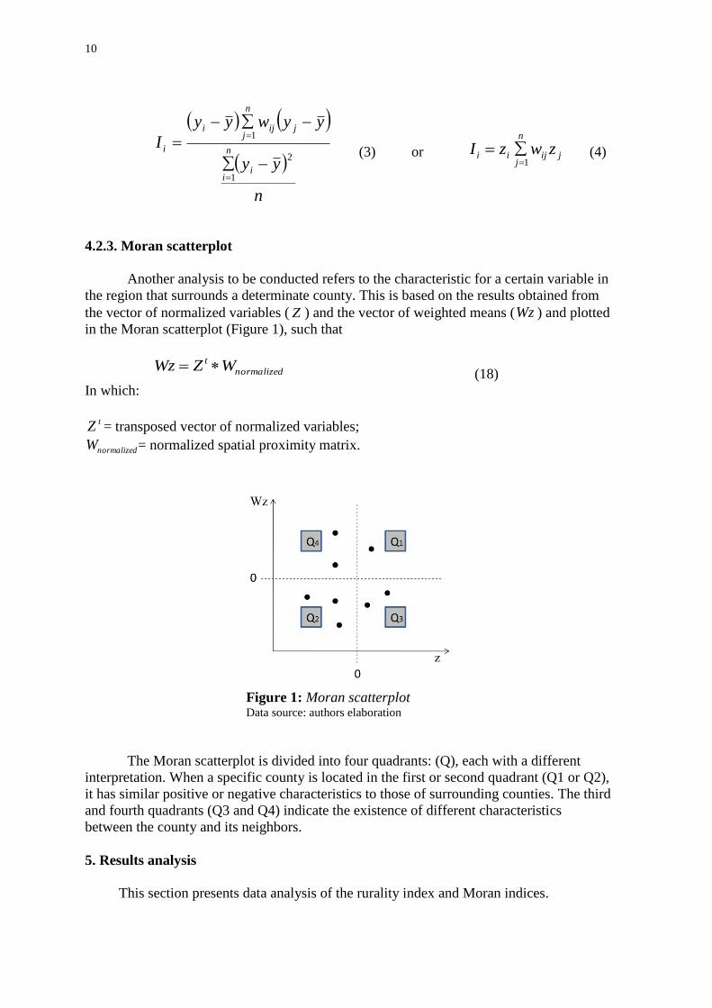
4.2.3. Moran scatterplot
Another analysis to be conducted refers to the characteristic for a certain variable in
the region that surrounds a determinate county. This is based on the results obtained from
the vector of normalized variables ( Z ) and the vector of weighted means (Wz ) and plotted
in the Moran scatterplot (Figure 1), such that
normalized
t WZWz (18)
In which:
tZ = transposed vector of normalized variables;
normalizedW = normalized spatial proximity matrix.
Figure 1: Moran scatterplot Data source: authors elaboration
The Moran scatterplot is divided into four quadrants: (Q), each with a different
interpretation. When a specific county is located in the first or second quadrant (Q1 or Q2),
it has similar positive or negative characteristics to those of surrounding counties. The third
and fourth quadrants (Q3 and Q4) indicate the existence of different characteristics
between the county and its neighbors.
5. Results analysis
This section presents data analysis of the rurality index and Moran indices.
11
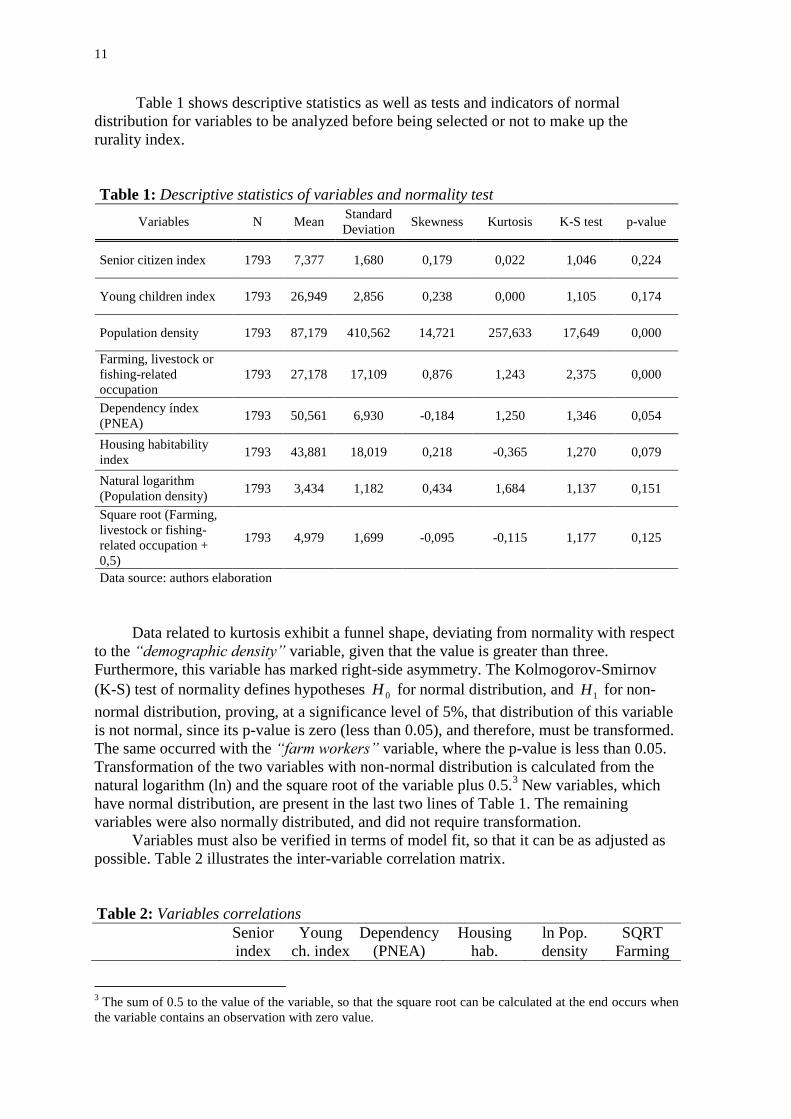
Table 1 shows descriptive statistics as well as tests and indicators of normal
distribution for variables to be analyzed before being selected or not to make up the
rurality index.
Table 1: Descriptive statistics of variables and normality test
Variables N Mean Standard
Deviation Skewness Kurtosis K-S test p-value
Senior citizen index 1793 7,377 1,680 0,179 0,022 1,046 0,224
Young children index 1793 26,949 2,856 0,238 0,000 1,105 0,174
Population density 1793 87,179 410,562 14,721 257,633 17,649 0,000
Farming, livestock or
fishing-related
occupation
1793 27,178 17,109 0,876 1,243 2,375 0,000
Dependency índex
(PNEA) 1793 50,561 6,930 -0,184 1,250 1,346 0,054
Housing habitability
index 1793 43,881 18,019 0,218 -0,365 1,270 0,079
Natural logarithm
(Population density) 1793 3,434 1,182 0,434 1,684 1,137 0,151
Square root (Farming,
livestock or fishing-
related occupation +
0,5)
1793 4,979 1,699 -0,095 -0,115 1,177 0,125
Data source: authors elaboration
Data related to kurtosis exhibit a funnel shape, deviating from normality with respect
to the “demographic density” variable, given that the value is greater than three.
Furthermore, this variable has marked right-side asymmetry. The Kolmogorov-Smirnov
(K-S) test of normality defines hypotheses 0H for normal distribution, and 1H for non-
normal distribution, proving, at a significance level of 5%, that distribution of this variable
is not normal, since its p-value is zero (less than 0.05), and therefore, must be transformed.
The same occurred with the “farm workers” variable, where the p-value is less than 0.05.
Transformation of the two variables with non-normal distribution is calculated from the
natural logarithm (ln) and the square root of the variable plus 0.5.3 New variables, which
have normal distribution, are present in the last two lines of Table 1. The remaining
variables were also normally distributed, and did not require transformation.
Variables must also be verified in terms of model fit, so that it can be as adjusted as
possible. Table 2 illustrates the inter-variable correlation matrix.
Table 2: Variables correlations
Senior
index
Young
ch. index
Dependency
(PNEA)
Housing
hab.
ln Pop.
density
SQRT
Farming
3 The sum of 0.5 to the value of the variable, so that the square root can be calculated at the end occurs when
the variable contains an observation with zero value.
12
Senior index 1,00 -0,47 0,04 -0,10 -0,01 0,16
Young ch. index -0,47 1,00 0,02 0,53 -0,30 0,23
Depend. (PNEA) 0,04 0,02 1,00 -0,03 -0,09 -0,12
Housing hab. -0,10 0,53 -0,03 1,00 -0,60 0,69
ln Pop. density -0,01 -0,30 -0,09 -0,60 1,00 -0,54
SQRT Farming 0,16 0,23 -0,12 0,69 -0,54 1,00 Data source: authors elaboration
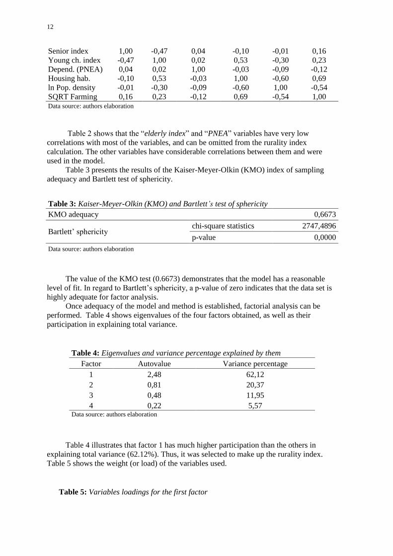
Table 2 shows that the “elderly index” and “PNEA” variables have very low
correlations with most of the variables, and can be omitted from the rurality index
calculation. The other variables have considerable correlations between them and were
used in the model.
Table 3 presents the results of the Kaiser-Meyer-Olkin (KMO) index of sampling
adequacy and Bartlett test of sphericity.
Table 3: Kaiser-Meyer-Olkin (KMO) and Bartlett’s test of sphericity
KMO adequacy 0,6673
Bartlett’ sphericity chi-square statistics 2747,4896
p-value 0,0000
Data source: authors elaboration
The value of the KMO test (0.6673) demonstrates that the model has a reasonable
level of fit. In regard to Bartlett’s sphericity, a p-value of zero indicates that the data set is
highly adequate for factor analysis.
Once adequacy of the model and method is established, factorial analysis can be
performed. Table 4 shows eigenvalues of the four factors obtained, as well as their
participation in explaining total variance.
Table 4: Eigenvalues and variance percentage explained by them
Factor Autovalue Variance percentage
1 2,48 62,12
2 0,81 20,37
3 0,48 11,95
4 0,22 5,57 Data source: authors elaboration
Table 4 illustrates that factor 1 has much higher participation than the others in
explaining total variance (62.12%). Thus, it was selected to make up the rurality index.
Table 5 shows the weight (or load) of the variables used.
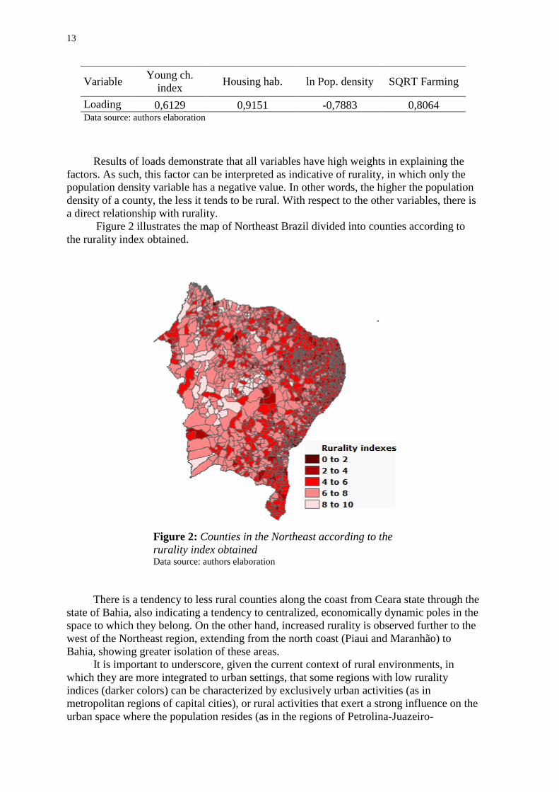
Table 5: Variables loadings for the first factor
13
Variable Young ch.
index Housing hab. ln Pop. density SQRT Farming
Loading 0,6129 0,9151 -0,7883 0,8064 Data source: authors elaboration
Results of loads demonstrate that all variables have high weights in explaining the
factors. As such, this factor can be interpreted as indicative of rurality, in which only the
population density variable has a negative value. In other words, the higher the population
density of a county, the less it tends to be rural. With respect to the other variables, there is
a direct relationship with rurality.
Figure 2 illustrates the map of Northeast Brazil divided into counties according to
the rurality index obtained.
Figure 2: Counties in the Northeast according to the
rurality index obtained Data source: authors elaboration
There is a tendency to less rural counties along the coast from Ceara state through the
state of Bahia, also indicating a tendency to centralized, economically dynamic poles in the
space to which they belong. On the other hand, increased rurality is observed further to the
west of the Northeast region, extending from the north coast (Piaui and Maranhão) to
Bahia, showing greater isolation of these areas.
It is important to underscore, given the current context of rural environments, in
which they are more integrated to urban settings, that some regions with low rurality
indices (darker colors) can be characterized by exclusively urban activities (as in
metropolitan regions of capital cities), or rural activities that exert a strong influence on the
urban space where the population resides (as in the regions of Petrolina-Juazeiro-
14
Sobradinho, in Pernambuco and Bahia; Açu-Mossoro, in Rio Grande do Norte; Campina
Grande, in Paraiba; Sobral, in Ceara; among others), as well as greater economic
dynamism.
Table 6 gives the ranking of the ten most rural and ten least rural counties in the
Northeast region.
Table 6: Ranking of the ten most rural and ten least rural counties in the Northeast
Ranking More rural Less rural
Municipality State Municipality State
1st Guaribas Piauí
Campina Grande Paraíba
2nd Betânia do Piauí Piauí
Toritama Pernambuco
3rd Curral Novo do Piauí Piauí
Itabuna Bahia
4th Morro Cabeça no Tempo Piauí
Carpina Pernambuco
5th Nova Santa Rita Piauí
Juazeiro do Norte Ceará
6th Capitão Gervásio Oliveira Piauí
Patos Paraíba
7th Brejo de Areia Maranhão
Caruaru Pernambuco
8th Caraúbas do Piauí Piauí
Feira de Santana Bahia
9th Fernando Falcão Maranhão
Nazaré da Mata Pernambuco
10th Formosa da Serra Negra Maranhão
Guarabira Paraíba
Data source: authors elaboration
Obs.: counties in the metropolitan regions of capital cities and Fernando de Noronha were not
considered.
Table 6 shows a predominance of counties from Piaui and Maranhão as the most
rural, signaling greater lack of infrastructure and isolation than other northeastern states.
On the other hand, less rural counties (excluding those with predominantly urban
characteristics, belonging to the metropolitan regions of capital cities) are located mostly in
the states of Pernambuco, Paraiba and Bahia, possibly demonstrating the existence of more
poles centralizing regional activities, which are essential to promoting greater dynamism.
The global Moran index obtained is considerable (0.57) and the p-value is less than
0.01. Thus, the null hypothesis is rejected, that is, there is a strong indication of spatial
correlation between counties in Northeast Brazil, with respect to rurality (or lack of
rurality), at a significance level of 5%. This correlation is also positive, indicating a
tendency to the formation of clusters composed of counties with similar characteristics
(very rural counties with very rural counties, or less rural with less rural). On the other
hand, there is no tendency to dependency relationships between counties with different
characteristics (very rural counties with less rural ones). In figure 1, this positive spatial
correlation can be identified by the fact that more rural counties are closer to one another
and to their less rural counterparts.
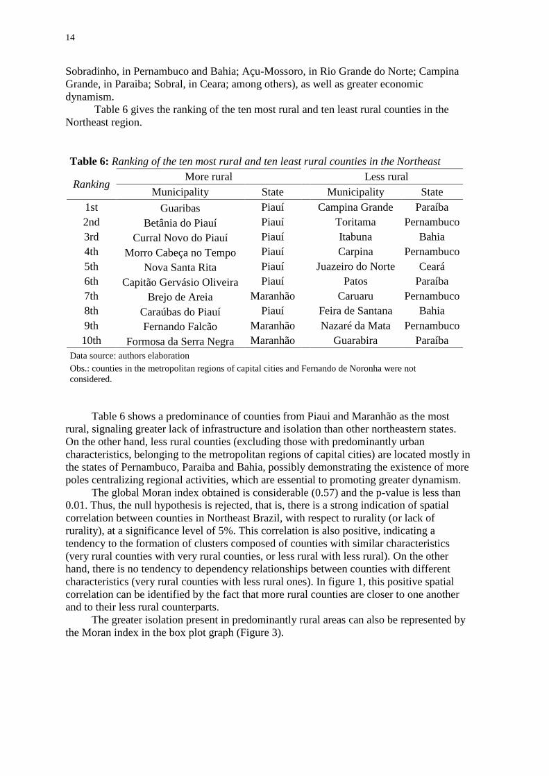
The greater isolation present in predominantly rural areas can also be represented by
the Moran index in the box plot graph (Figure 3).
15
Figure 3: Box plot graph of local Moran indices in counties of the Northeast Data source: authors elaboration
Outliers are composed almost entirely of counties belonging to the metropolitan
regions of capital cities, exhibiting very high spatial correlations. On the other hand, the
more rural counties, which make up the greater part of the Northeast, are present in the box
plot, at correlations close to zero, showing more isolation. This can also be demonstrated in
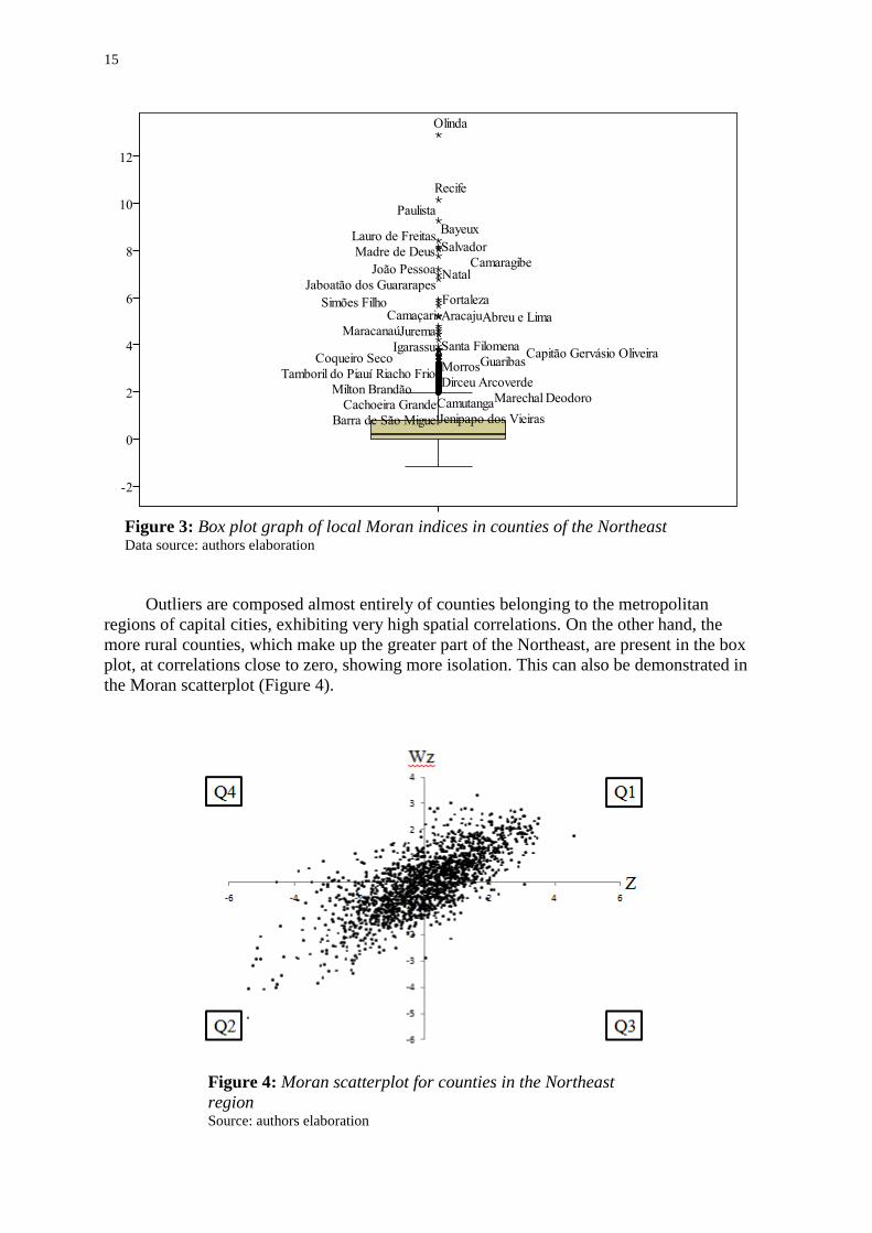
the Moran scatterplot (Figure 4).
Figure 4: Moran scatterplot for counties in the Northeast
region Source: authors elaboration
16
In this case, points that are more distant from the origin represent counties with
greater correlation with their neighbors. The second quadrant (Q2) contains counties
farthest from the origin. These exhibit predominantly urban traits and are surrounded by
counties with similar characteristics, as seen primarily in metropolitan regions of state
capitals. In the first quadrant (Q1) predominantly rural counties are found, surrounded by
others with similar characteristics. Counties are not as far from the origin, since their
spatial correlations are lower. The third and fourth quadrant (Q3 and Q4, respectively)
contain counties with different characteristics from their neighbors, that is, predominantly
rural surrounded by predominantly urban and vice versa. In this case, there are fewer
counties, with generally very low correlations.
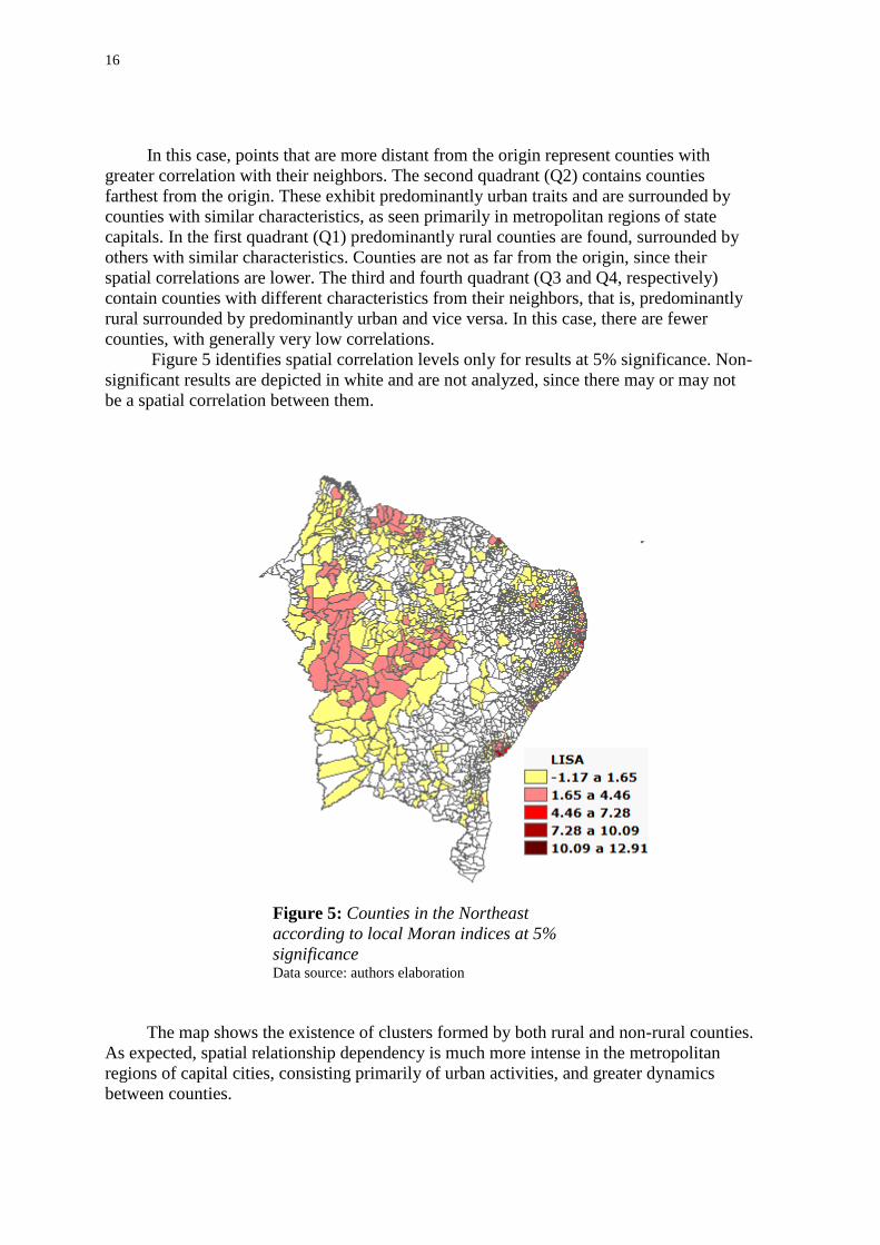
Figure 5 identifies spatial correlation levels only for results at 5% significance. Non-
significant results are depicted in white and are not analyzed, since there may or may not
be a spatial correlation between them.
Figure 5: Counties in the Northeast
according to local Moran indices at 5%
significance Data source: authors elaboration
The map shows the existence of clusters formed by both rural and non-rural counties.
As expected, spatial relationship dependency is much more intense in the metropolitan
regions of capital cities, consisting primarily of urban activities, and greater dynamics
between counties.
17
The yellow counties have low correlations with those surrounding them. With
respect to more rural counties, there is a large cluster in the midwest part of the region,
encompassing several counties in Maranhão, Piauí and Bahia, such as Mirador-MA,
Gilbués-PI, Monte Alegre do Piauí-PI, Pilão Arcado-BA, and Campo Alegre de Lourdes-
BA, among others. Just above is another cluster, in the state of Maranhão, formed by
counties such as Arame and Itaipava do Grajaú. On the coast of this state is another group,
composed of counties such as Barreirinhas and Humberto de Campos. There are other
smaller clusters, such as near Caruaru-PE, Caicó-RN, and Itabuna-BA, among others.
6. Final considerations
This study discussed current tendencies of rural environments, not only in Brazil, but
throughout the world, as well as their importance in forming territories. In light of the
predominantly insufficient economic reproduction in rural areas, through only agriculture,
greater interaction has increasingly been sought with urban regions at sufficient levels to
retain workers in rural regions. This “deruralization” of rural areas has increasingly
allowed inhabitants to take greater advantage of available urban structure including access
to education, better living and transport conditions, greater social and commercial
interaction, among others, without losing their rural identity. New activities also emerge
and intensify, such as those related to tourism, crafts and others. This reveals other
previously hidden qualities of rural environments, opening new possibilities and allowing
greater economic reproduction.
The growing dynamic observed in rural-urban and rural-rural relationships creates
conditions for the emergence of domains or clusters, which this study sought to elucidate
by analyzing counties in Northeastern Brazil.
First, we obtained a variable representing the rurality of counties through principal
component analysis, which demonstrated the rurality and isolation of cities in the entire
Northeast. The most significant portion of rural and isolated counties was found in Piauí
state, followed by Maranhão. On the other hand, the states of Pernambuco, Paraíba and
Bahia exhibited a greater number of less rural cities, which, although not characteristically
urban, may represent potential focal points for activities essential to regional development.
The Moran indices revealed a dependent structure between neighboring cities and,
consequently, of clusters. Purely urban clusters were identified in metropolitan regions,
which were more cohesive owing to their more consolidated dynamics and recognized as
outliers. In addition, less consolidated rural clusters were also observed at some sites in the
region.
In summary, the present study sought to identify, rural counties and the formation of
rural clusters in the Northeast, based on statistical multivariate analysis techniques and
spatial analysis. Such investigations are important in identifying dynamic and non-dynamic
rural areas essential in directing public policies aimed at rural development.
Nevertheless, our research contains a number of important limitations: first, the
generality of local problems are not analyzed in depth; second, variables used may not be
sufficient to clearly explain a phenomenon as complex as rurality; however, in order to
better fit tests performed in factorial analysis, it would be difficult to increase their number
without test results preventing the use of this method; finally, identification of clusters
through spatial correlation is limited for an in-depth understanding of spatial relationships
between counties.
18
References
Abramovay, R. (1999) Agricultura familiar e desenvolvimento territorial, Reforma Agrária
– Revista da Associação Brasileira da Reforma Agrária, v. 28. n. 1.
______ (2000), O capital social dos territórios: repensando o desenvolvimento rural,
Economia Aplicada, v. IV, p. 379-397, São Paulo.
Andrade, M. C. de (1987), Espaço, Polarização e Desenvolvimento – uma introdução à
economia regional, Editora Atlas S.A., São Paulo.
Anselin, L. (1995), Local Indicators of Spatial Association – LISA, Geographical
Analysis, v. 27, n. 2, p. 93-115.
Belmar, E., Loguercio, N. (2006), Ordenamiento Territorial: Una Herramienta para el
Desarrollo Rural Sostenible, FAO.
Cazella, A. A., Bonnal, P., Maluf, R. S. (2009), Multifuncionalidade da Agricultura
Familiar no Brasil e o Enfoque da Pesquisa, em Cazella, A. A., Bonnal, P. e Maluf, R.
S. (coord.), Agricultura Familiar: multifuncionalidade e desenvolvimento territorial no
Brasil, Mauad X, v. 1, pp. 47-70, Rio de Janeiro.
Gama, R. G., Strauch, J. C. M. (2009), Análise espacial de indicadores de
Desenvolvimento Sustentável: Aplicação do índice de Moran, Proceedings os 12
Congresso de Geógrafos de America Latina, Montevidéu.
Gordillo de Anda, G. (1997) Restructuración institucional y revalorización de los vínculos
rural-urbanos, Seminario Internacional Interrelación Rural-Urbana Y Desarrollo
Descentralizado, FAO/ONU, Taxco, México.
Graziano da Silva, J. (1997), O Novo Rural Brasileiro. Nova Economia, v.7, n. 1, p. 43-81.
Graziano da Silva, J., del Grossi, M. E. (2001), O Novo Rural Brasileiro, em Graziano da
Silva, J. (coord.), Ocupações rurais não-agrícolas: Oficina de atualização temática,
Londrina, Brasil.
Hair, J. F., Anderson, R. E., Tatham, R. L. E., Black, W. C. (1998), Multivariate data
analysis, New York: Prentice Hall.
Harvey, D. (2005), A produção capitalista do espaço. São Paulo: Anna Blume.
INEA – Istituto Nazionale di Economia Agraria, Tipologie di aree rurali in Italia, Studi &
Ricerche, INEA, Roma.
Kageyama, A. A. (2008), Desenvolvimento rural: conceitos e aplicação ao caso brasileiro,
UFRGS, v.1, Porto Alegre.
Kinsella, J., Wilson, S., de Jong, F., Renting, H. (2000), Pluriactivity as a Livelihood
Strategy in Irish Farm Households and its Role in Rural Development, Sociologia
Ruralis, v. 40, n. 4, pp. 481-496.
19
Ministério do Desenvolvimento Agrário – MDA. <http://www.mda.gov.br>, Acesso em
2011.
Neves, M. C., Ramos, F. R., Câmara, G., Monteiro, A. M. V., Camargo, E. C. G. (2000),
Análise exploratória espacial de dados socioeconômicos de São Paulo, em Gisbrasil
2000, Salvador.
Ocaña-Riola, R., Sánchez-Cantalejo, C. (2005), Rurality Index for small areas in Spain,
Social Indicators Research, n. 73, pp. 247-266.
Perroux, F. (1967), A economia do século XX, Herber, Lisboa.
Van der Ploeg, J. D., Renting, H., Brunori, G., Knickel, K., Mannion, J., Marsden, T., de
Roest, K., Sevilla-Guzmán, E., Ventura, F. (2000), Rural Development: From Practices
and Policies towards Theory, Sociologia Ruralis, v. 40, n. 4, pp. 391-408.
Veiga, J. E. da (2003), Cidades Imaginárias – O Brasil é menos urbano do que se calcula,
Editora Autores Associados, Campinas, Brasil.
______ (2001), O Brasil rural ainda não encontrou seu eixo de desenvolvimento, Estudos
Avançados, v. 15, n. 43, pp. 101-119.
Wiggins, S., Proctor, S. (2001), How special are rural areas? The economic implications of
locations for rural development, Development Policy Review, v. 19, n. 4, pp. 427-436.