Embed Size (px)
Citation preview
Rural, remote and regional differences in women’s health: Findings from the Australian Longitudinal Study on Women’s Health
Final report prepared for the Australian Government Department of Health and AgeingJune 2011
Authors:Annette Dobson, Julie Byles, Xenia Dolja-Gore, David Fitzgerald, Richard Hockey, Deborah Loxton, Deirdre McLaughlin, Nancy Pachana, Jenny Powers, Jane Rich, David Sibbritt and Leigh Tooth
Major Report F
Rural, remote and regional differences in women’s health: Findings from the Australian
Longitudinal Study on Women’s Health
The research on which this report is based was conducted as part of the Australian Longitudinal Study on
Women‘s Health by the University of Newcastle and the University of Queensland. We are grateful to the
Australian Government Department of Health and Ageing for funding and to the women who provided the
survey data. We acknowledge Medicare Australia for providing any Pharmaceutical Benefits Scheme
and Medicare Benefits Scheme data.
- ii -
Table of Contents
1. Executive summary....................................................................................................................................... 1
2. Introduction ................................................................................................................................................. 5
2.1. Introduction to ALSWH ............................................................................................................................... 5 2.2. Area of residence in the ALSWH ................................................................................................................. 7
2.2.1. Measure of Remoteness: ARIA+ ............................................................................................................. 7 2.2.2. Location of ALSWH participants........................................................................................................... 10
2.3. References ................................................................................................................................................ 14
3. Differences in health status by geographic location .................................................................................... 15
3.1. Mortality ................................................................................................................................................... 15 3.2. Risk factors ............................................................................................................................................... 17
3.2.1. Introduction ......................................................................................................................................... 17 3.2.2. Chronic conditions ................................................................................................................................ 23 3.2.3. SF36 scores ........................................................................................................................................... 29
3.3. Summary ................................................................................................................................................... 29 3.4. References ................................................................................................................................................ 32
4. Access to, use of, and satisfaction with health services by geographic location .......................................... 33
4.1. Selected usage, access, satisfaction- health services. .............................................................................. 33 4.1.1. Visits to GPs ......................................................................................................................................... 33 4.1.2. Satisfaction with access to GP services ................................................................................................ 36 4.1.3. Visits to Medical Specialists ................................................................................................................. 40 4.1.4. Satisfaction with access to medical specialists .................................................................................... 42 4.1.5. Hospital Admissions ............................................................................................................................. 44 4.1.6. Self-reported procedures ..................................................................................................................... 46
4.2. The management of heart conditions in older rural and urban Australian women................................. 49 4.2.1. Health Service Use ............................................................................................................................... 49 4.2.2. Medication Use .................................................................................................................................... 54 4.2.3. Self-management advice ..................................................................................................................... 55 4.2.4. References ............................................................................................................................................ 57
4.3. Use of dental services ............................................................................................................................... 58 4.3.1. Discussion ............................................................................................................................................ 64 4.3.2. References ............................................................................................................................................ 65
4.4. Complementary and alternative medicine (CAM) .................................................................................... 66 4.4.1. Introduction ......................................................................................................................................... 66 4.4.2. Consultations with conventional health care providers by CAM use ................................................... 66 4.4.3. Rating of conventional health care providers by CAM use .................................................................. 67 4.4.4. Symptoms and diagnoses by CAM use ................................................................................................. 68 4.4.5. Diseases and consultations with a CAM practitioner ........................................................................... 69 4.4.6. Summary .............................................................................................................................................. 70 4.4.7. References ............................................................................................................................................ 71
4.5. The use of CAM in the 1921-26 birth cohort: Rural women speak out .................................................... 72 4.6. Screening services .................................................................................................................................... 74
4.6.1. Pap tests .............................................................................................................................................. 74 4.6.2. Mammograms ..................................................................................................................................... 81 4.6.3. Discussion ............................................................................................................................................ 85
- iii -
5. Out of pocket costs for medical services by geographic location ................................................................ 86
5.1. Introduction .............................................................................................................................................. 86 5.2. Discussion ................................................................................................................................................. 92 5.3. Conclusion ................................................................................................................................................ 93 5.4. References: ............................................................................................................................................... 93
6. Differences in birth interventions by geographic location........................................................................... 94
6.1. Introduction .............................................................................................................................................. 94 6.2. Birth interventions by area of residence .................................................................................................. 94 6.3. Risk factors for having an epidural or spinal block ................................................................................... 96 6.4. Risk factors for having a caesarean .......................................................................................................... 98 6.5. Key issues: ................................................................................................................................................ 99
7. Climate events and women’s health ......................................................................................................... 100
7.1. Exceptional circumstances and mental health ....................................................................................... 100 7.2. Precipitation and self rated health ......................................................................................................... 102 7.3. Soil salinity .............................................................................................................................................. 105 7.4. Qualitative experience of drought ......................................................................................................... 107
7.4.1. Drought as a burden .......................................................................................................................... 108 7.4.2. Ageing in drought .............................................................................................................................. 108 7.4.3. Resilience during drought .................................................................................................................. 109 7.4.4. Conclusion .......................................................................................................................................... 109
7.5. References .............................................................................................................................................. 110
8. Social cohesion ......................................................................................................................................... 111
8.1. Neighbourhood....................................................................................................................................... 111 8.1.1. Neighbourhood connection................................................................................................................ 111 8.1.2. Neighbourhood safety ....................................................................................................................... 112 8.1.3. Neighbourhood attachment and trust ............................................................................................... 113 8.1.4. Social support..................................................................................................................................... 114 8.1.5. Life satisfaction .................................................................................................................................. 115 8.1.6. Stress .................................................................................................................................................. 116 8.1.7. Perceived control ............................................................................................................................... 117 8.1.8. Optimism............................................................................................................................................ 118 8.1.9. References .......................................................................................................................................... 118
8.2. Cohesion/satisfaction ............................................................................................................................. 119 8.2.1. Introduction ....................................................................................................................................... 119 8.2.2. References .......................................................................................................................................... 121
8.3. Driving..................................................................................................................................................... 122 8.3.1. Introduction ....................................................................................................................................... 122 8.3.2. Main means of transport ................................................................................................................... 122 8.3.3. Factors associated with continuing to drive ...................................................................................... 123 8.3.4. Discussion .......................................................................................................................................... 124 8.3.5. References .......................................................................................................................................... 125
- iv -
List of Tables
Table 2-1 Schedule of surveys for the ALSWH, ......................................................................................................... 6 Table 2-2 Survey 1 Unweighted Frequencies by ARIA+ Categories ......................................................................... 10 Table 2-3 Survey 1 Weighted Frequencies by ARIA+ Categories ............................................................................. 11 Table 2-4 Area distribution of women in the Australian population and the ALSWH sample in 1996. ................... 11 Table 2-5 ALSWH Sample Weights ........................................................................................................................... 11 Table 2-6 RRMA ARIA+ Classes, weighted Frequencies and Row Percents ............................................................. 12 Table 2-7 Attrition at Survey 5 by Area of Residence, Frequencies and Row Percents ........................................... 13 Table 3-1 Numbers (and column percentages) of women categorised by area of residence, survival
or cause of death. .................................................................................................................................... 15 Table 3-2 Hazard ratios (adjusted for age) of deaths from all causes and selected causes. .................................... 16 Table 4-1 Medication usage recorded by women reporting doctor diagnosed ischaemic heart
disease, heart failure or atrial fibrillation. ............................................................................................... 55 Table 4-2 Self management advice received by women reporting doctor diagnosed ischaemic heart
disease, heart failure or atrial fibrillation. ............................................................................................... 56 Table 4-3 Adjusted† odds ratios and associated 95% confidence intervals (C.I.) .................................................... 61 Table 4-4 Factors associated with dentist consultations by older Australian women, derived from a
longitudinal analysis using multivariable generalized estimation equation(GEE) modelling with backward stepwise elimination (n=9,387) ....................................................................................... 63
Table 4-5 Consultations with conventional health care providers by CAM use (consulted with a CAM practitioner or not) ......................................................................................................................... 67
Table 4-6 Rating of conventional health care providers by CAM use (consulted with a CAM practitioner or not) Level of Satisfaction (1=excellent … 5=poor). .......................................................... 68
Table 4-7 Sought help for symptoms by CAM use (consulted with a CAM practitioner or not) .............................. 69 Table 4-8 Diagnoses by CAM user status (consulted with a CAM practitioner or not) ............................................ 70 Table 4-9 Factors associated with having a Pap test in the past 2 years. 1973-78 and 1946-51
cohorts. .................................................................................................................................................... 80 Table 4-10 Factors associated with having a mammogram in the past 2 years. 1946-51 cohort. ............................ 84 Table 5-1 Proportions of women with zero out of pocket costs for general practitioner services in
2008 ......................................................................................................................................................... 92 Table 7-1 Regression models for mental health component scores in the 1973-1978 cohort:
coefficients with confidence intervals that do not include zero are statistically significant. ................ 106 Table 7-2 Regression models for mental health component scores in the 1946-1951 cohort:
coefficients with confidence intervals that do not include zero are statistically significant. ................ 106 Table 7-3 Regression models for mental health component scores in the 1921-1926 cohort:
coefficients with confidence intervals that do not include zero are statistically significant. ................ 107 Table 8-1 Factors affecting odds of driving, over time and across areas ............................................................... 124
- v -
List of Figures
Figure 2-1 Map of Australia showing the 2006 ARIA+ categories ............................................................................ 9 Figure 2-2 Map of Australia showing locations of the ALSWH participants (2006) ................................................. 9 Figure 3-1 Current smoking in the 1973-78 cohort and the 1946-51 cohort. ........................................................ 18 Figure 3-2 Smoking in the 1921-26 cohort. ............................................................................................................ 19 Figure 3-3 Obesity in all cohorts. ............................................................................................................................ 21 Figure 3-4 Non/low physical activity in all ALSWH cohorts. ................................................................................... 22 Figure 3-5 Prevalence and incidence of diabetes by area of residence. ................................................................ 24 Figure 3-6 Prevalence and incidence of hypertension by area of residence.......................................................... 25 Figure 3-7 Prevalence and incidence of asthma by area of residence. .................................................................. 26 Figure 3-8 Prevalence and incidence of chronic obstructive pulmonary disease by area of
residence in the 1921-26 cohort. .......................................................................................................... 27 Figure 3-9 Prevalence and incidence of osteoporosis by area of residence, 1921-26 cohort and
1946-51 cohort. ..................................................................................................................................... 28 Figure 3-10 Physical Component Score by area of residence. .................................................................................. 30 Figure 3-11 Mental Component Score by area of residence. ................................................................................... 31 Figure 4-1 Proportions of women making 7 or more visits to a GP – 1973-78 cohort ........................................... 33 Figure 4-2 Proportions of women making 7 or more visits to a GP – 1946-51 cohort ........................................... 34 Figure 4-3 Proportions of women making 7 or more visits to a GP – 1921-26 cohort ........................................... 35 Figure 4-4 Satisfaction with access to GP services – 1973-78 cohort at Survey 5. ................................................. 37 Figure 4-5 Satisfaction with access to GP services for 1945-51 cohort at Survey 5. ............................................... 38 Figure 4-6 Satisfaction with GP Services for 1921-26 cohort at Survey 3. .............................................................. 39 Figure 4-7 Proportion of women who had visited a specialist in the past year – 1973-78 cohort ......................... 40 Figure 4-8 Proportion of women who had visited a specialist in the past year – 1946-51 cohort. ........................ 41 Figure 4-9 Proportion of women who had visited a specialist in the past year – 1921-26 cohort. ........................ 41 Figure 4-10 Satisfaction with access to medical specialists at Survey 5 – 1973-78 cohort. ...................................... 42 Figure 4-11 Satisfaction with access to medical specialists/hospital at Survey 5 - 1946-51 cohort. ........................ 43 Figure 4-12 Satisfaction with access to medical specialist/hospital at Survey 3 – 1921-26 cohort. ........................ 43 Figure 4-13 Self-reported admissions to hospitals – 1921-26 cohort. ...................................................................... 44 Figure 4-14 Satisfaction with access to hospitals for the ALSWH 1921-26 cohort, by area of
residence. .............................................................................................................................................. 45 Figure 4-15 Satisfaction with access to hospitals for the ALSWH 1946-51 cohort, by area of
residence. .............................................................................................................................................. 45 Figure 4-16 Satisfaction with access to hospitals for the ALSWH 1973-78 cohort, by area of
residence. .............................................................................................................................................. 46 Figure 4-17 Self report of hysterectomy, by area of residence – 1946-51 cohort. ................................................... 47 Figure 4-18 Self report of cholecystectomy, by area of residence – 1946-51 cohort. .............................................. 47 Figure 4-19 Self report of hip surgery by area of residence – 1921-26 cohort. ........................................................ 48 Figure 4-20 Health Service Use for women with Ischaemic Heart Disease according to area of
residence. .............................................................................................................................................. 50 Figure 4-21 Health Service Use for women with Heart Failure according to area of residence. .............................. 52 Figure 4-22. Health Service Use for women with Atrial Fibrillation according to area of residence. ........................ 53 Figure 4-23 1973-78 cohort Surveys 4 and 5, visited a dentist. ................................................................................ 58 Figure 4-24 1946-51 cohort, visited a dentist Surveys 2-5. ...................................................................................... 59 Figure 4-25 1921-26 cohort, visited a dentist, Surveys 2-4. ..................................................................................... 59 Figure 4-26 Self report of time since last Pap test by women in 1973-78 cohort at Surveys 1-5 ............................. 75 Figure 4-27 Proportions of women in the 1946-51 cohort who report having a hysterectomy by
each survey and by area of residence. .................................................................................................. 76 Figure 4-28 Self report of time since last Pap test by women in the 1946-51 cohort. ............................................. 77 Figure 4-29 Ease of obtaining a Pap test. 1973-78 cohort Survey 5 ......................................................................... 78 Figure 4-30 Ease of obtaining a Pap test. 1946-51 cohort Survey 5 ......................................................................... 78 Figure 4-31 Self report of time since last Mammogram by women in 1946-51 cohort. .......................................... 82
- vi -
Figure 4-32 Ease of obtaining a Mammogram. 1946-51 cohort Survey 5 ................................................................. 83 Figure 5-1 Out of pocket costs for GP services since 1995-2001. ............................................................................. 87 Figure 5-2 Mean out-of pocket cost per general practice consultation per woman per year, 2002-
2008, for women born in 1921-26 by area of residence, adjusted to 2008 dollar values. ...................... 89 Figure 5-3 Mean out-of pocket cost per general practice consultation per woman per year, 2002-
2008, for women born in 1946-51 by area of residence, adjusted to 2008 dollar values. ...................... 90 Figure 5-4 Mean out-of pocket cost per general practice consultation per woman per year, 2002-
2008, for women born in 1973-78 by area of residence, adjusted to 2008 dollar values. ...................... 91 Figure 6-1 Prolonged labour by area of residence. .................................................................................................... 94 Figure 6-2 Emotional distress by area of residence ................................................................................................... 95 Figure 6-3 Type of pain relief by area of residence ................................................................................................... 95 Figure 6-4 Type of delivery by area of residence ....................................................................................................... 95 Figure 6-5 Episiotomy or vaginal tear requiring stitches by area of residence .......................................................... 96 Figure 6-6 Epidural or spinal block by age of first-time mother ................................................................................ 97 Figure 6-7 Epidural or spinal block by private health insurance ................................................................................ 97 Figure 6-8 Epidural or spinal block by body mass index group .................................................................................. 97 Figure 6-9 Epidural or spinal block by height ............................................................................................................. 98 Figure 7-1 Distribution of women living in Exceptional Circumstances declared areas by ARIA+ ........................... 100 Figure 7-2 Ability to manage on available income by Exceptional Circumstances .................................................. 101 Figure 7-3 Level of optimism for women living in Exceptional Circumstances and non-Exceptional
Circumstances area ................................................................................................................................ 101 Figure 7-4 Distribution of dryness and drought across Australia by Survey year for the 1946-51
cohort. .................................................................................................................................................... 102 Figure 7-5 Ability to manage on available income by dryness and drought in 2007 for ALSWH
participants in the 1946-51 cohort. ....................................................................................................... 103 Figure 7-6 Level of social support by dryness and drought in 2007 for ALSWH participants in the
1946-51 cohort. ..................................................................................................................................... 103 Figure 7-7 Level of optimism by dryness and drought in 2007 for ALSWH participants in the 1946-51
cohort. .................................................................................................................................................... 104 Figure 7-8 Changes in General Health over time by dryness and drought for ALSWH participants in
the 1946-51 cohort. ............................................................................................................................... 104 Figure 7-9 Changes in Mental Health over time by dryness and drought for ALSWH participants in
the 1946-51 cohort. ............................................................................................................................... 105 Figure 8-1 Mean neighbourhood connection scores and 95% confidence intervals in each
geographic location ............................................................................................................................... 111 Figure 8-2 Mean neighbourhood safety scores and 95% confidence intervals in each geographic
location .................................................................................................................................................. 112 Figure 8-3 Mean neighbourhood attachment & trust scores and 95% confidence intervals location .................... 113 Figure 8-4 Proportion of women reporting level of social support in each geographic location ............................ 114 Figure 8-5 Mean life satisfaction scores and 95% confidence intervals in each geographic location ..................... 115 Figure 8-6 Proportion of women reporting levels of stress in each geographic location ........................................ 116 Figure 8-7 Mean perceived life control scores and 95% confidence intervals in each geographic
location .................................................................................................................................................. 117 Figure 8-8 Mean optimism scores and 95% confidence intervals in each geographic location .............................. 118 Figure 8-9 Main means of transport for women in major cities, regional, and remote areas at Survey
3 (N= 7966), Survey 4 (N=6197) and Survey 5 (N=4772) ....................................................................... 123
1
1. Executive summary
Introduction
Much has been published about rural health disadvantage in Australia, including a series of reports by the
Australian Institute of Health and Welfare (AIHW). The AIHW concludes: ―... it is not currently possible to
apportion the generally poorer health outcomes outside major cities to access, environment or risk factor
issues. It is likely that each of these three play a part.‖ (AIHW, 2011)
The Australian Longitudinal Study on Women‘s Health (ALSWH) is well-placed to elucidate these reasons
using detailed data provided by women from across Australia. ALSWH is funded by the Australian
Government Department of Health and Ageing and conducted by the University of Newcastle and the
University of Queensland. ALSWH participants have taken part in five surveys over 15 years and many
have consented to use of linked data from Medicare Australia.
The findings reported here can be summarised in three broad themes:
Generally poorer health of women living in regional and remote areas;
Differences in access to and use of a wide range of health services;
The resilience of rural women and characteristics of life in rural communities which ameliorate
sometimes difficult conditions.
It is important to note that within each of these themes there are contradictions and inconsistencies in the
findings, and these emphasise the need for further research to allow deeper understanding and more
nuanced responses. The study findings also show clear examples where government policies have been
effective in reducing health inequities, as well as highlighting situations in which changes in policies and
practices could lead to further improvements.
This summary is structured around these three themes, drawing on findings from throughout the report.
Poorer health of rural women
Among ALSWH participants born in 1921-26, 23% died between 1996 and 2006. Consistent with the
findings of others, death rates for these women were higher in regional and remote areas than in major
cities. The regional and remote death rates for women in the 1921-26 cohort were particularly higher for
lung cancer, chronic obstructive pulmonary disease and ischaemic heart disease, which are often
associated with tobacco smoking (section 3.1). (There were too few deaths in the other cohorts to
provide reliable estimates).
When we examined the main risk factors for major diseases for women from all cohorts we found that
current smoking prevalence was not markedly different across areas defined by distance from major
centres. In all areas and age groups smoking decreased over time, although the change was slower
among young women in remote areas. The explanation for the higher death rates from apparently
smoking-related causes among older rural women may therefore lie in higher levels of smoking in the
past (possibly decades ago), exposure to smoking by others, or greater exposure to other hazards
(section 3.2.1).
For women of all ages, one health risk factor that was consistently higher with increasing distance from
major cities was obesity. Prevalence and incidence of diabetes and hypertension, conditions which are
associated with obesity, were also consistently higher. When we analysed the rates of these conditions
- 2 -
by area, body mass index (BMI), and various demographic factors, the area differences in disease could
be almost entirely explained by the higher levels of obesity.
The ALSWH data strongly suggest that higher levels of BMI (and prevalence of obesity) in regional and
remote areas account for the higher rates of diabetes and other risk factors for cardiovascular disease.
This is an area where effective health promotion targeted to rural women could reduce health inequality.
For various other health-related conditions there were few differences in prevalence or trends in incidence
across areas; these included asthma (section 3.2.2), and prolonged labour or emotional distress among
first-time mothers (section 6).
Access to and use of health services
Use of most health services was higher in major cities than in regional and remote areas. However the
pattern of GP use among the 1973-78 and 1946-51 cohorts varied over time. For the period 1996 - 2002
the level of bulk billing decreased and out-of-pocket costs increased for all age cohorts, especially for
women in rural areas (section 5). In 2004, there were changes to Medicare reimbursements to GPs for
services to patients from rural and remote areas, selected eligible metropolitan areas, or anywhere in
Tasmania, and for services provided to older people (section 5). When we analysed bulk-billing rates and
out-of-pocket costs for 2002-2008 we found an overall improvement in access to bulk-billing. We also
found continuing relative disadvantage for women living in inner regional areas not covered by the 2004
Medicare change. These results suggest that the incentives should be further evaluated to assess the
potential for reducing inequity for inner regional areas while maintaining the improved access for people
in more remote areas.
Numbers of visits to specialists decreased with increasing distance from major cities for all age cohorts at
all surveys (section 4.1.3). However there was little difference in hospital admissions between areas
(section 4.1.5). A detailed analysis of medical care for women with heart disease showed lower levels of
recent cardiological review, echocardiograms and stress tests for rural women. Medications consistent
with recommended guidelines and advice for self-management of their conditions was generally poor but
consistent across areas (section 4.2).
Among the 1946-51 cohort rates of hysterectomy increased with distance from major cities (section
4.1.6). This pattern persisted over time and seems likely to reflect less access to or less interest in trying
alternative treatments by women in country areas.
In contrast to the pattern for hysterectomies in the 1946-51 cohort, rates of other procedures generally
decreased with distance from major centres. This was the pattern for hip surgery in the 1921-26 cohort at
Survey 2, although the inequality for hip surgery was reduced over time (section 4.1.6). For both the
1946-51 cohort and the 1921-26 cohorts, osteoporosis was more commonly reported in major cities, as
the diagnosis depends on tests more easily available there (section 3.2.2). In the 1973-78 cohort, there
was consistently greater use of obstetric interventions in major cities than in regional and remote areas;
these included use of epidural injections, forceps or ventous suction, and emergency and elective
caesarean section (section 6).
Visits to dentists for women in all cohorts were much more common in major cities (section 4.3). Detailed
analyses – both cross-sectional and longitudinal, with adjustments for socio-economic and demographic
factors and health status – showed almost 50% higher use of dentists by women in cities compared to
rural areas. However, overall, only 35% of women in the 1921-26 cohort had visited a dentist in a 12
month period; women cited access difficulties, including travel and costs, as reasons for not visiting a
dentist even when they needed to do so. The cost of private dental care, compared with Medicare
subsidised medical treatment, is a barrier to appropriate oral health care and this has recently been
- 3 -
identified as a top priority by the Health and Hospital Reform Commission (National Health and Hospitals
Reform Commission, 2009).
In contrast to other health services, Pap tests and mammography were more uniformly used across areas
with breast screening rates highest in remote areas and Pap test rates highest in regional areas (section
4.6).
At each survey women are asked to rate their access to and their satisfaction with services. The results
were consistent across all cohorts, over time and for all services. Women in remote areas experienced
the greatest difficulty accessing services (even when their use is relatively high, as for screening tests).
Women in regional areas experienced more difficulties accessing services than women in major cities.
This pattern was true for access to GPs (GPs who bulk-bill, female GPs, after hours service, hours when
GPs are available, waiting times for appointments, and choice of GPs – section 4.1.2); access to
specialists (section 4.1.4); hospitals (section4.1.5); and screening tests (section 4.6).
In summary, for most medical and other health services, use is much lower in remote and regional areas
and women experience considerably more difficulties with access than in major cities. Country women
whose health is generally poorer than city women‘s also have less health care. The exceptions to this
pattern – publically funded screening services and changes in bulk-billing policy – show that government
subsidies for health services can be very effective ways of reducing inequities in health services.
Resilience and life in rural communities
Despite the well-documented differences in objective measures of health across areas, physical and
mental health scores based on self-reported data differed little, even though the expected differences
between age cohorts and over time were apparent (section 3.2.3). This may reflect differences in views,
values and expectations related to health among rural women compared to women living in major cities.
Use of complementary and alternative medicines (CAM) is higher in regional and remote areas (section
4.4). CAM use does not appear to be related to health status (sections 4.4.4 and 4.4.5) and there is
conflicting evidence about whether it is related to dissatisfaction with conventional health services
(sections 4.4.2, 4.4.3 and 4.5). Interviews with a small sample of rural women revealed some scepticism
about conventional practitioners and belief in traditional practises and CAM, reinforced by the social
networks in rural areas.
We examined several markers of climate change and their potential impact on health in rural areas.
These were: the declaration of areas as experiencing exceptional circumstances (e.g., drought, flood and
fire) that result in severe downturn in farm and farm-related income and entitle some people in these
areas to income support from governments (section 7.1); long-term changes in rainfall resulting in
prolonged periods of dryness and drought (section 7.2); and soil salinity, and markers of temperature and
vegetation in south-western Western Australia (section 7.3). In all cases we found no evidence of adverse
effects on mental or physical health. Analysis of comments written by women on the surveys pointed to
the resilience and adaptability of country women to dealing with adversity (perhaps strengthened by
government support) as the possible explanation (section 7.4).
ALSWH has included several measures of neighbourhood satisfaction, social support, life satisfaction
optimism and stress (section 8.1). These showed considerable differences between regional, remote and
urban areas. Scores for neighbourhood connectedness, feeling safe and life satisfaction were highest in
remote areas and decreased with increasing nearness to major cities. Neighbourhood attachment and
trust were highest in outer and inner regional areas and lowest in major cities. Scores for perceived
control and optimism were highest in remote areas and lowest in outer regional areas. Interviews with
older women emphasised the importance of support from neighbours and social networks for women
- 4 -
living in rural areas, and on driving as the main means of transport which is essential to maintain these
connections (section 8.2).
Women in regional and remote areas have few transport options other than driving and they continue to
drive as long as their health and vision permit (section 8.3). Services to help rural people maintain good
vision are especially important for their independence and community connectedness. The importance of
driving for rural people to access health care and other services for themselves and the people they
provide care for, and to maintain social their networks poses a policy challenge. Stopping older people
from driving because of health issues which affect their ability to drive, while potentially reducing road
crashes, impacts adversely on many aspects of their lives, especially in rural and remote areas. This is a
complex issue. Consideration should be given to vehicle and road design that is safer for older people;
alternative transport options and supportive infrastructures; effective licensing systems for older drivers;
and driver education tools.
Overall, the report shows a number of differences in health and health-care use for women in regional
and remote areas compared to urban-dwelling women. The findings point to the need to address specific
risk factors such as obesity, and to continue, strengthen and broaden existing effective policies for better
access to services. It is also important to consider the contexts in which women live, and how these
impact on women‘s mental and social well-being.
References
Australian Institute of Health and Welfare. Impact of rurality on health status,
http://www.aihw.gov.au/rural-health-impact-of-rurality/ (accessed 16 March, 2011).
National Health and Hospitals Reform Commission. 2009. A Healthier Future for all Australians – Final
Report of the National Health and Hospitals Reform Commission. Commonwealth Government of
Australia. ISBN: 1-74186-940-4
- 5 -
2. Introduction
In 2007-2008 the Australian Institute of Health and Welfare (AIHW) published a series of reports
documenting differences in health status and health systems performance (AIHW 2007; 2008a; 2008b).
AIHW found death rates are lower and other measures of health status are better for people living in
major cities in Australia than for those living in regional or remote areas, and concluded ―it is not currently
possible to apportion the generally poorer health outcomes outside major cities to access, environment or
risk factor issues. It is likely that each of these three play a part.‖ Other researchers have also found that
differences in health between people living in regional and rural areas compared to urban areas in
Australia are complicated, with different patterns for different health conditions (Smith et al., 2008;
Vagenas et al., 2009; Jong et al., 2004). Comparisons with other countries are complicated because
patterns vary depending on the extent of geographic isolation, access to services (including health
insurance coverage), and occupational hazards (Smith et al., 2008; Judd et al., 2002).
Most commonly cited reasons for poorer health in rural and regional areas of Australia include:
lower socio-economic level (e.g., less education, lower income);
higher proportions of people of Aboriginal and Torres Strait Islander background:
different attitudes to health and health services (e.g., greater resilience or stoicism);
less healthy lifestyle (e.g., higher prevalence of smoking and overweight);
environmental and occupational exposures (e.g., dust, drought, sun exposure);
poorer access to health services (e.g., distance to services, greater out-of-pocket costs);
less effective health services (e.g., hospital with poorer facilities, less experienced doctors).
The challenge is to disentangle these factors. To meet this challenge we need:
data on health outcomes for each individual (to avoid the ‗ecological fallacy‘ of making inferences about individuals based on evidence from aggregate data);
data on each of the relevant factors (‗exposures‘) for the same individual (in order to estimate the joint effects of exposures);
longitudinal data in order to identify ‗causes‘ that occur before the ‗effects‘ (to avoid ‗reverse causation‘ interpretation);
knowledge of risk factors and management of the selected conditions in order to identify points along the disease pathway which are potentially amenable to changes;
understanding of the extent to which interventions could reduce the urban-rural differences.
In this report, we use accumulated data from ALSWH participants to examine some of these issues.
2.1. Introduction to ALSWH
The ALSWH is a longitudinal population-based survey funded by the Australian Government Department
of Health and Ageing. The project began in 1996 and involves three large, nationally representative,
cohorts of Australian women representing three generations:
the 1973-1978 cohort, aged 18 to 23 years when first recruited in 1996 (N=14 247) and now aged 33 to 38 years in 2011
- 6 -
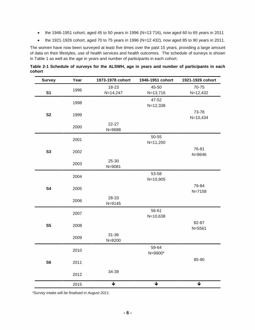
the 1946-1951 cohort, aged 45 to 50 years in 1996 (N=13 716), now aged 60 to 65 years in 2011
the 1921-1926 cohort, aged 70 to 75 years in 1996 (N=12 432), now aged 85 to 90 years in 2011.
The women have now been surveyed at least five times over the past 15 years, providing a large amount
of data on their lifestyles, use of health services and health outcomes. The schedule of surveys is shown
in Table 1 as well as the age in years and number of participants in each cohort.
Table 2-1 Schedule of surveys for the ALSWH, age in years and number of participants in each cohort
Survey Year 1973-1978 cohort 1946-1951 cohort 1921-1926 cohort
S1 1996
18-23
N=14,247
45-50
N=13,716
70-75
N=12,432
1998 47-52
N=12,338
S2 1999 73-78
N=10,434
2000 22-27
N=9688
2001 50-55
N=11,200
S3 2002 76-81
N=8646
2003 25-30
N=9081
2004 53-58
N=10,905
S4 2005 79-84
N=7158
2006 28-33
N=9145
2007 56-61
N=10,638
S5 2008 82-87
N=5561
2009 31-36
N=8200
2010 59-64
N=9900*
S6 2011 85-90
2012 34-39
2015
*Survey intake will be finalised in August 2011.
- 7 -
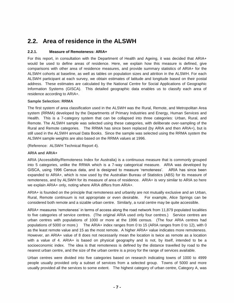
2.2. Area of residence in the ALSWH
2.2.1. Measure of Remoteness: ARIA+
For this report, in consultation with the Department of Health and Ageing, it was decided that ARIA+
would be used to define areas of residence. Here, we explain how this measure is defined, give
comparisons with other area of residence measures, and provide summary statistics of ARIA+ for the
ALSWH cohorts at baseline, as well as tables on population sizes and attrition in the ALSWH. For each
ALSWH participant at each survey, we obtain estimates of latitude and longitude based on their postal
address. These estimates are calculated by the National Centre for Social Applications of Geographic
Information Systems (GISCA). This detailed geographic data enables us to classify each area of
residence according to ARIA+.
Sample Selection: RRMA
The first system of area classification used in the ALSWH was the Rural, Remote, and Metropolitan Area
system (RRMA) developed by the Departments of Primary Industries and Energy, Human Services and
Health. This is a 7-category system that can be collapsed into three categories: Urban, Rural, and
Remote. The ALSWH sample was selected using these categories, with deliberate over-sampling of the
Rural and Remote categories. The RRMA has since been replaced (by ARIA and then ARIA+), but is
still used in the ALSWH annual Data Books. Since the sample was selected using the RRMA system the
ALSWH sample weights are also based on the RRMA values at 1996.
(Reference: ALSWH Technical Report 4).
ARIA and ARIA+
ARIA (Accessibility/Remoteness Index for Australia) is a continuous measure that is commonly grouped
into 5 categories, unlike the RRMA which is a 7-way categorical measure. ARIA was developed by
GISCA, using 1996 Census data, and is designed to measure ‗remoteness‘. ARIA has since been
expanded to ARIA+, which is now used by the Australian Bureau of Statistics (ABS) for its measure of
remoteness, and by ALSWH for its measure of area of residence. ARIA+ is very similar to ARIA so here
we explain ARIA+ only, noting where ARIA differs from ARIA+.
ARIA+ is founded on the principle that remoteness and urbanity are not mutually exclusive and an Urban,
Rural, Remote continuum is not appropriate or even desirable. For example, Alice Springs can be
considered both remote and a sizable urban centre. Similarly, a rural centre may be quite accessible.
ARIA+ measures ‗remoteness‘ in terms of access along the road network from 11,879 populated localities
to five categories of service centres. (The original ARIA used only four centres.) Service centres are
urban centres with populations of 1000 or more at the 1996 census. (The four ARIA centres had
populations of 5000 or more.) The ARIA+ index ranges from 0 to 15 (ARIA ranges from 0 to 12), with 0
as the least remote value and 15 as the most remote. A higher ARIA+ value indicates more remoteness.
However, an ARIA+ value of 8 does not necessarily mean the location is twice as remote as a location
with a value of 4. ARIA+ is based on physical geography and is not, by itself, intended to be a
socioeconomic index. The idea is that remoteness is defined by the distance travelled by road to the
nearest urban centre, and the size of the urban centre is a proxy for the range of services available.
Urban centres were divided into five categories based on research indicating towns of 1000 to 4999
people usually provided only a subset of services from a selected group. Towns of 5000 and more
usually provided all the services to some extent. The highest category of urban centre, Category A, was
- 8 -
a centre where all services are fully available. There are 738 service centres used in the ARIA+
methodology.
The ARIA+ score for a particular locality is calculated by first measuring the shortest road distance from a
populated locality to each of the nearest five categories of service centre. Towns within a service centre
are given a distance of zero. Also, the Australian average (mean) of these road distances, for each
category, is calculated. For each locality the ratio of the shortest distance to the national average
shortest distance, for each category of service centre, is calculated. This gives five ratios for each
category of service centre. The maximum values for these ratios are capped at three. The five individual
values are then summed to arrive at a single ARIA+ score for the populated locality. This is necessarily
from 0 to 15 inclusive.
Localities on islands had their distances adjusted. Anyone living within one of the 11,879 localities can
be assigned an ARIA+ score from this method. For those living outside the localities, a 1 km by 1 km grid
method is used. Each such grid in Australia is given an ARIA+ value based on the scores from the six
closest localities. The grid‘s ARIA+ value is given to anyone living within the grid.
(Reference: http://gisca.adelaide.edu.au/projects/category/about_aria.html)
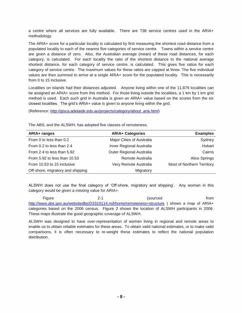
The ABS, and the ALSWH, has adopted five classes of remoteness.
ARIA+ ranges ARIA+ Categories Examples
From 0 to less than 0.2 Major Cities of Australia Sydney
From 0.2 to less than 2.4 Inner Regional Australia Hobart
From 2.4 to less than 5.92 Outer Regional Australia Cairns
From 5.92 to less than 10.53 Remote Australia Alice Springs
From 10.53 to 15 inclusive Very Remote Australia Most of Northern Territory
Off-shore, migratory and shipping Migratory
ALSWH does not use the final category of ‗Off-shore, migratory and shipping‘. Any woman in this
category would be given a missing value for ARIA+.
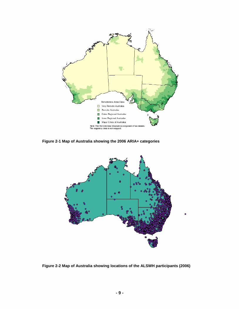
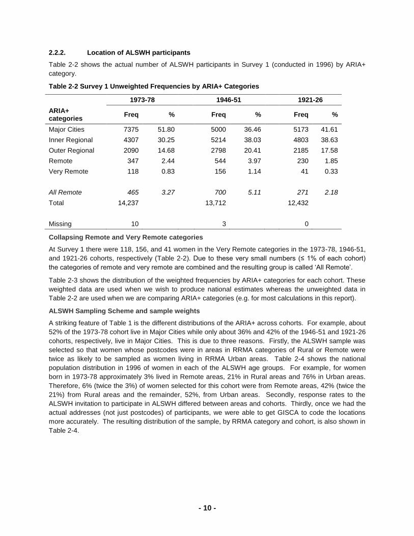
Figure 2-1 (sourced from
http://www.abs.gov.au/websitedbs/D3310114.nsf/home/remoteness+structure ) shows a map of ARIA+
categories based on the 2006 census. Figure 2 shows the location of ALSWH participants in 2006.
These maps illustrate the good geographic coverage of ALSWH.
ALSWH was designed to have over-representation of women living in regional and remote areas to
enable us to obtain reliable estimates for these areas. To obtain valid national estimates, or to make valid
comparisons, it is often necessary to re-weight these estimates to reflect the national population
distribution.
- 9 -
Figure 2-1 Map of Australia showing the 2006 ARIA+ categories
Figure 2-2 Map of Australia showing locations of the ALSWH participants (2006)
- 10 -
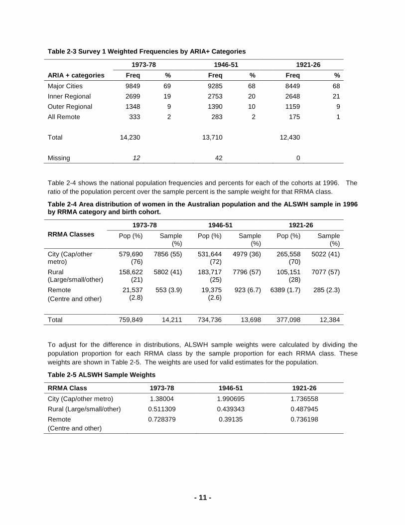
2.2.2. Location of ALSWH participants
Table 2-2 shows the actual number of ALSWH participants in Survey 1 (conducted in 1996) by ARIA+
category.
Table 2-2 Survey 1 Unweighted Frequencies by ARIA+ Categories
1973-78 1946-51 1921-26
ARIA+ categories
Freq %
Freq %
Freq %
Major Cities 7375 51.80 5000 36.46 5173 41.61
Inner Regional 4307 30.25 5214 38.03 4803 38.63
Outer Regional 2090 14.68 2798 20.41 2185 17.58
Remote 347 2.44 544 3.97 230 1.85
Very Remote 118 0.83 156 1.14 41 0.33
All Remote 465 3.27 700 5.11 271 2.18
Total 14,237 13,712 12,432
Missing 10 3 0
Collapsing Remote and Very Remote categories
At Survey 1 there were 118, 156, and 41 women in the Very Remote categories in the 1973-78, 1946-51,
and 1921-26 cohorts, respectively (Table 2-2). Due to these very small numbers (≤ 1% of each cohort)
the categories of remote and very remote are combined and the resulting group is called ‗All Remote‘.
Table 2-3 shows the distribution of the weighted frequencies by ARIA+ categories for each cohort. These
weighted data are used when we wish to produce national estimates whereas the unweighted data in
Table 2-2 are used when we are comparing ARIA+ categories (e.g. for most calculations in this report).
ALSWH Sampling Scheme and sample weights
A striking feature of Table 1 is the different distributions of the ARIA+ across cohorts. For example, about
52% of the 1973-78 cohort live in Major Cities while only about 36% and 42% of the 1946-51 and 1921-26
cohorts, respectively, live in Major Cities. This is due to three reasons. Firstly, the ALSWH sample was
selected so that women whose postcodes were in areas in RRMA categories of Rural or Remote were
twice as likely to be sampled as women living in RRMA Urban areas. Table 2-4 shows the national
population distribution in 1996 of women in each of the ALSWH age groups. For example, for women
born in 1973-78 approximately 3% lived in Remote areas, 21% in Rural areas and 76% in Urban areas.
Therefore, 6% (twice the 3%) of women selected for this cohort were from Remote areas, 42% (twice the
21%) from Rural areas and the remainder, 52%, from Urban areas. Secondly, response rates to the
ALSWH invitation to participate in ALSWH differed between areas and cohorts. Thirdly, once we had the
actual addresses (not just postcodes) of participants, we were able to get GISCA to code the locations
more accurately. The resulting distribution of the sample, by RRMA category and cohort, is also shown in
Table 2-4.
- 11 -
Table 2-3 Survey 1 Weighted Frequencies by ARIA+ Categories
1973-78 1946-51 1921-26
ARIA + categories Freq % Freq % Freq %
Major Cities 9849 69 9285 68 8449 68
Inner Regional 2699 19 2753 20 2648 21
Outer Regional 1348 9 1390 10 1159 9
All Remote 333 2 283 2 175 1
Total 14,230 13,710 12,430
Missing 12 42 0
Table 2-4 shows the national population frequencies and percents for each of the cohorts at 1996. The
ratio of the population percent over the sample percent is the sample weight for that RRMA class.
Table 2-4 Area distribution of women in the Australian population and the ALSWH sample in 1996 by RRMA category and birth cohort.
RRMA Classes
1973-78 1946-51 1921-26
Pop (%) Sample (%)
Pop (%) Sample (%)
Pop (%) Sample (%)
City (Cap/other metro)
579,690 (76)
7856 (55) 531,644 (72)
4979 (36) 265,558 (70)
5022 (41)
Rural (Large/small/other)
158,622 (21)
5802 (41) 183,717 (25)
7796 (57) 105,151 (28)
7077 (57)
Remote
(Centre and other)
21,537 (2.8)
553 (3.9) 19,375 (2.6)
923 (6.7) 6389 (1.7) 285 (2.3)
Total 759,849 14,211 734,736 13,698 377,098 12,384
To adjust for the difference in distributions, ALSWH sample weights were calculated by dividing the
population proportion for each RRMA class by the sample proportion for each RRMA class. These
weights are shown in Table 2-5. The weights are used for valid estimates for the population.
Table 2-5 ALSWH Sample Weights
RRMA Class 1973-78 1946-51 1921-26
City (Cap/other metro) 1.38004 1.990695 1.736558
Rural (Large/small/other) 0.511309 0.439343 0.487945
Remote
(Centre and other)
0.728379 0.39135 0.736198
- 12 -
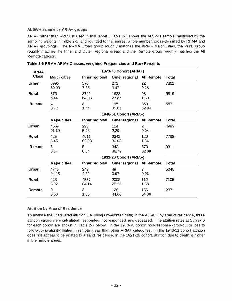
ALSWH sample by ARIA+ groups
ARIA+ rather than RRMA is used in this report. Table 2-6 shows the ALSWH sample, multiplied by the
sampling weights in Table 2-5 and rounded to the nearest whole number, cross-classified by RRMA and
ARIA+ groupings. The RRMA Urban group roughly matches the ARIA+ Major Cities, the Rural group
roughly matches the Inner and Outer Regional areas, and the Remote group roughly matches the All
Remote category.
Table 2-6 RRMA ARIA+ Classes, weighted Frequencies and Row Percents
RRMA Class
1973-78 Cohort (ARIA+)
Major cities Inner regional Outer regional All Remote Total
Urban 6996 89.00
570 7.25
273 3.47
22 0.28
7861
Rural 375 6.44
3729 64.08
1622 27.87
93 1.60
5819
Remote 4 0.72
8 1.44
195 35.01
350 62.84
557
1946-51 Cohort (ARIA+)
Major cities Inner regional Outer regional All Remote Total
Urban 4569 91.69
298 5.98
114 2.29
2 0.04
4983
Rural 425 5.45
4911 62.98
2342 30.03
120 1.54
7798
Remote 6 0.64
5 0.54
342 36.73
578 62.08
931
1921-26 Cohort (ARIA+)
Major cities Inner regional Outer regional All Remote Total
Urban 4745 94.15
243 4.82
49 0.97
3 0.06
5040
Rural 428 6.02
4557 64.14
2008 28.26
112 1.58
7105
Remote 0 0.00
3 1.05
128 44.60
156 54.36
287
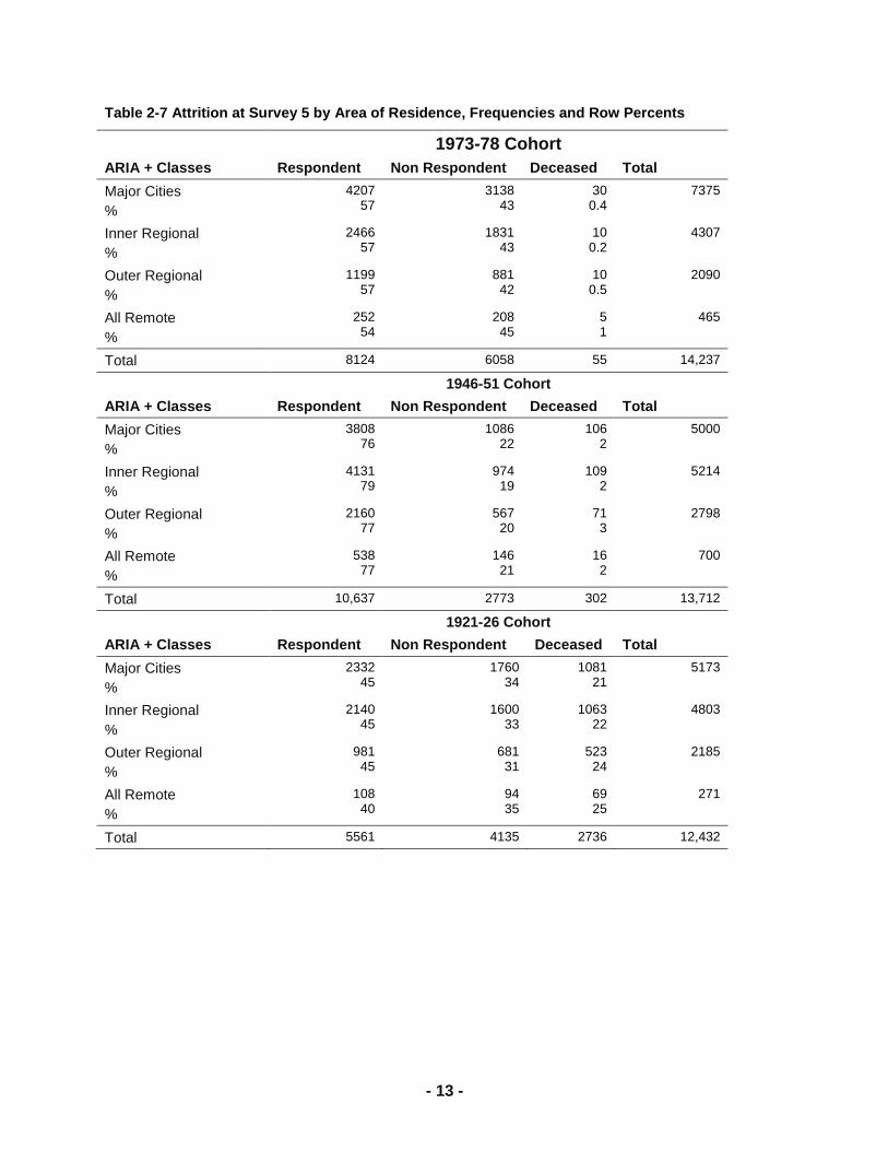
Attrition by Area of Residence
To analyse the unadjusted attrition (i.e. using unweighted data) in the ALSWH by area of residence, three
attrition values were calculated: responded, not responded, and deceased. The attrition rates at Survey 5
for each cohort are shown in Table 2-7 below. In the 1973-78 cohort non-response (drop-out or loss to
follow-up) is slightly higher in remote areas than other ARIA+ categories. In the 1946-51 cohort attrition
does not appear to be related to area of residence. In the 1921-26 cohort, attrition due to death is higher
in the remote areas.
- 13 -
Table 2-7 Attrition at Survey 5 by Area of Residence, Frequencies and Row Percents
1973-78 Cohort
ARIA + Classes Respondent Non Respondent Deceased Total
Major Cities
%
4207 57
3138 43
30 0.4
7375
Inner Regional
%
2466 57
1831 43
10 0.2
4307
Outer Regional
%
1199 57
881 42
10 0.5
2090
All Remote
%
252 54
208 45
5 1
465
Total 8124 6058 55 14,237
1946-51 Cohort
ARIA + Classes Respondent Non Respondent Deceased Total
Major Cities
%
3808 76
1086 22
106 2
5000
Inner Regional
%
4131 79
974 19
109 2
5214
Outer Regional
%
2160 77
567 20
71 3
2798
All Remote
%
538 77
146 21
16 2
700
Total 10,637 2773 302 13,712
1921-26 Cohort
ARIA + Classes Respondent Non Respondent Deceased Total
Major Cities
%
2332 45
1760 34
1081 21
5173
Inner Regional
%
2140 45
1600 33
1063 22
4803
Outer Regional
%
981 45
681 31
523 24
2185
All Remote
%
108 40
94 35
69 25
271
Total 5561 4135 2736 12,432
- 14 -
2.3. References
Australian Institute of Health and Welfare. (2007). Rural, regional and remote health: A study on mortality
(2nd edition). Rural Health Series (Australian Institute of Health and Welfare, Canberra).
Australian Institute of Health and Welfare. (2008a). Rural, regional and remote health: Indicators of health
status and determinants of health. Rural Health Series (Australian Institute of Health and Welfare,
Canberra).
Australian Institute of Health and Welfare. (2008b). Rural, regional and remote health: Indicators of health
system performance. Rural Health Series (Australian Institute of Health and Welfare Canberra).
Smith, K.B., Humphreys, J.S. & Wilson, M.G.A. (2008). Addressing the health disadvantage of rural
populations: How does epidemiological evidence inform rural health policies and research?
Australian Journal of Rural Health 16, 56-66.
Vagenas, D., McLaughlin, D. & Dobson, A. (2009). Regional variation in the health of older Australian
women: Grey canaries? Australian and New Zealand Journal of Public Health 33, 119-125.
Jong, K.E., Smith, D.P., Yu, X.Q., O'Connell, D.L., Goldstein, D. & Armstrong, B.K. (2004). Remoteness
of residence and survival from cancer in New South Wales. Medical Journal of Australia 180, 618-
622.
Judd, F.K., Jackson, H.J., Komiti, A., Murray, G., Hodgins, G. & Fraser, C. (2002). High prevalence
disorders in urban and rural communities. Australian and New Zealand Journal of Psychiatry 36,
104-113.
- 15 -
3. Differences in health status by
geographic location
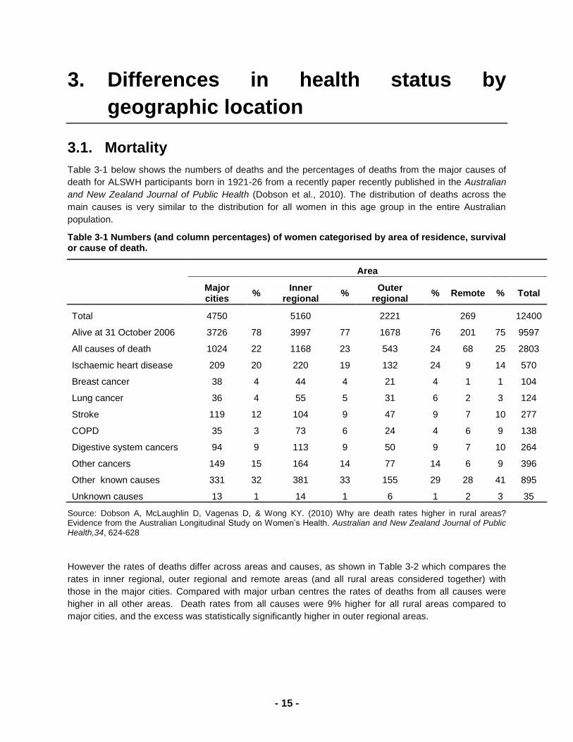
3.1. Mortality
Table 3-1 below shows the numbers of deaths and the percentages of deaths from the major causes of
death for ALSWH participants born in 1921-26 from a recently paper recently published in the Australian
and New Zealand Journal of Public Health (Dobson et al., 2010). The distribution of deaths across the
main causes is very similar to the distribution for all women in this age group in the entire Australian
population.
Table 3-1 Numbers (and column percentages) of women categorised by area of residence, survival or cause of death.
Area
Major cities
% Inner
regional %
Outer regional
% Remote % Total
Total 4750
5160
2221
269
12400
Alive at 31 October 2006 3726 78 3997 77 1678 76 201 75 9597
All causes of death 1024 22 1168 23 543 24 68 25 2803
Ischaemic heart disease 209 20 220 19 132 24 9 14 570
Breast cancer 38 4 44 4 21 4 1 1 104
Lung cancer 36 4 55 5 31 6 2 3 124
Stroke 119 12 104 9 47 9 7 10 277
COPD 35 3 73 6 24 4 6 9 138
Digestive system cancers 94 9 113 9 50 9 7 10 264
Other cancers 149 15 164 14 77 14 6 9 396
Other known causes 331 32 381 33 155 29 28 41 895
Unknown causes 13 1 14 1 6 1 2 3 35
Source: Dobson A, McLaughlin D, Vagenas D, & Wong KY. (2010) Why are death rates higher in rural areas? Evidence from the Australian Longitudinal Study on Women‘s Health. Australian and New Zealand Journal of Public Health,34, 624-628
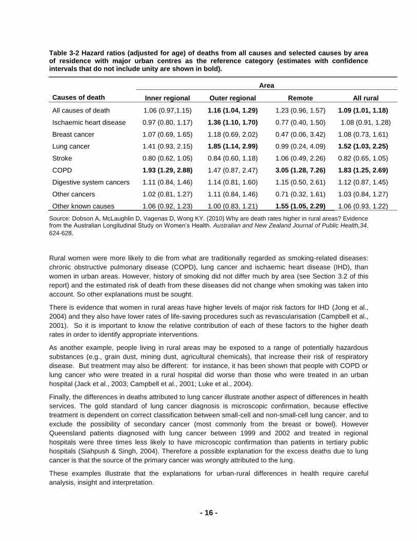
However the rates of deaths differ across areas and causes, as shown in Table 3-2 which compares the
rates in inner regional, outer regional and remote areas (and all rural areas considered together) with
those in the major cities. Compared with major urban centres the rates of deaths from all causes were
higher in all other areas. Death rates from all causes were 9% higher for all rural areas compared to
major cities, and the excess was statistically significantly higher in outer regional areas.
- 16 -
Table 3-2 Hazard ratios (adjusted for age) of deaths from all causes and selected causes by area of residence with major urban centres as the reference category (estimates with confidence intervals that do not include unity are shown in bold).
Causes of death
Area
Inner regional Outer regional Remote All rural
All causes of death 1.06 (0.97,1.15) 1.16 (1.04, 1.29) 1.23 (0.96, 1.57) 1.09 (1.01, 1.18)
Ischaemic heart disease 0.97 (0.80, 1.17) 1.36 (1.10, 1.70) 0.77 (0.40, 1.50) 1.08 (0.91, 1.28)
Breast cancer 1.07 (0.69, 1.65) 1.18 (0.69, 2.02) 0.47 (0.06, 3.42) 1.08 (0.73, 1.61)
Lung cancer 1.41 (0.93, 2.15) 1.85 (1.14, 2.99) 0.99 (0.24, 4.09) 1.52 (1.03, 2.25)
Stroke 0.80 (0.62, 1.05) 0.84 (0.60, 1.18) 1.06 (0.49, 2.26) 0.82 (0.65, 1.05)
COPD 1.93 (1.29, 2.88) 1.47 (0.87, 2.47) 3.05 (1.28, 7.26) 1.83 (1.25, 2.69)
Digestive system cancers 1.11 (0.84, 1.46) 1.14 (0.81, 1.60) 1.15 (0.50, 2.61) 1.12 (0.87, 1.45)
Other cancers 1.02 (0.81, 1.27) 1.11 (0.84, 1.46) 0.71 (0.32, 1.61) 1.03 (0.84, 1.27)
Other known causes 1.06 (0.92, 1.23) 1.00 (0.83, 1.21) 1.55 (1.05, 2.29) 1.06 (0.93, 1.22)
Source: Dobson A, McLaughlin D, Vagenas D, Wong KY. (2010) Why are death rates higher in rural areas? Evidence from the Australian Longitudinal Study on Women‘s Health. Australian and New Zealand Journal of Public Health,34,
624-628.
Rural women were more likely to die from what are traditionally regarded as smoking-related diseases:
chronic obstructive pulmonary disease (COPD), lung cancer and ischaemic heart disease (IHD), than
women in urban areas. However, history of smoking did not differ much by area (see Section 3.2 of this
report) and the estimated risk of death from these diseases did not change when smoking was taken into
account. So other explanations must be sought.
There is evidence that women in rural areas have higher levels of major risk factors for IHD (Jong et al.,
2004) and they also have lower rates of life-saving procedures such as revascularisation (Campbell et al.,
2001). So it is important to know the relative contribution of each of these factors to the higher death
rates in order to identify appropriate interventions.
As another example, people living in rural areas may be exposed to a range of potentially hazardous
substances (e.g., grain dust, mining dust, agricultural chemicals), that increase their risk of respiratory
disease. But treatment may also be different: for instance, it has been shown that people with COPD or
lung cancer who were treated in a rural hospital did worse than those who were treated in an urban
hospital (Jack et al., 2003; Campbell et al., 2001; Luke et al., 2004).
Finally, the differences in deaths attributed to lung cancer illustrate another aspect of differences in health
services. The gold standard of lung cancer diagnosis is microscopic confirmation, because effective
treatment is dependent on correct classification between small-cell and non-small-cell lung cancer, and to
exclude the possibility of secondary cancer (most commonly from the breast or bowel). However
Queensland patients diagnosed with lung cancer between 1999 and 2002 and treated in regional
hospitals were three times less likely to have microscopic confirmation than patients in tertiary public
hospitals (Siahpush & Singh, 2004). Therefore a possible explanation for the excess deaths due to lung
cancer is that the source of the primary cancer was wrongly attributed to the lung.
These examples illustrate that the explanations for urban-rural differences in health require careful
analysis, insight and interpretation.
- 17 -
3.2. Risk factors
3.2.1. Introduction
In this section we present the prevalence of selected risk factors at every survey for each of the five
ARIA+ categories and each cohort. For some risk factors questions were not asked at every survey (e.g.
smoking was only included in Surveys 1 and 2 for the 1921-26 cohort) or questions were asked differently
(eg. alcohol consumption in several surveys and/or cohorts and physical activity at Survey 1 for all
cohorts). The data are shown for least favourable levels of each risk factor: current smoking, obesity,
non/low physical activity.
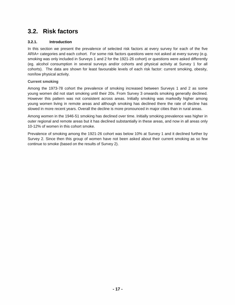
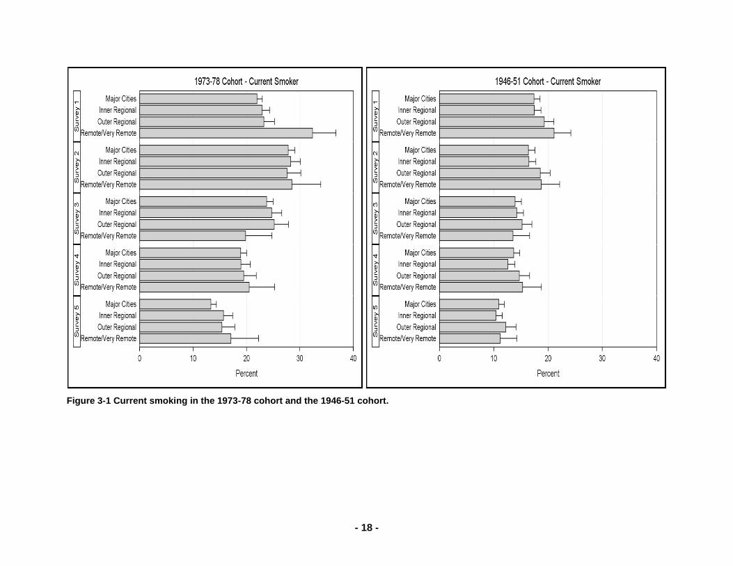
Current smoking
Among the 1973-78 cohort the prevalence of smoking increased between Surveys 1 and 2 as some
young women did not start smoking until their 20s. From Survey 3 onwards smoking generally declined.
However this pattern was not consistent across areas. Initially smoking was markedly higher among
young women living in remote areas and although smoking has declined there the rate of decline has
slowed in more recent years. Overall the decline is more pronounced in major cities than in rural areas.
Among women in the 1946-51 smoking has declined over time. Initially smoking prevalence was higher in
outer regional and remote areas but it has declined substantially in these areas, and now in all areas only
10-12% of women in this cohort smoke.
Prevalence of smoking among the 1921-26 cohort was below 10% at Survey 1 and it declined further by
Survey 2. Since then this group of women have not been asked about their current smoking as so few
continue to smoke (based on the results of Survey 2).
- 18 -
Figure 3-1 Current smoking in the 1973-78 cohort and the 1946-51 cohort.
- 19 -
Figure 3-2 Smoking in the 1921-26 cohort.
- 20 -
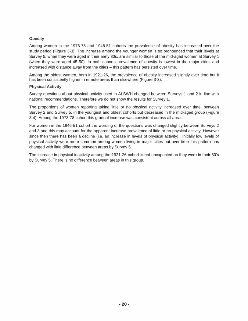
Obesity
Among women in the 1973-78 and 1946-51 cohorts the prevalence of obesity has increased over the
study period (Figure 3-3). The increase among the younger women is so pronounced that their levels at
Survey 5, when they were aged in their early 30s, are similar to those of the mid-aged women at Survey 1
(when they were aged 45-50). In both cohorts prevalence of obesity is lowest in the major cities and
increased with distance away from the cities – this pattern has persisted over time.
Among the oldest women, born in 1921-26, the prevalence of obesity increased slightly over time but it has been consistently higher in remote areas than elsewhere (Figure 3-3).
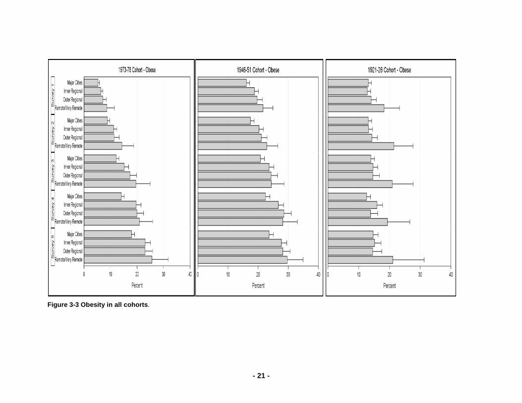
Physical Activity
Survey questions about physical activity used in ALSWH changed between Surveys 1 and 2 in line with
national recommendations. Therefore we do not show the results for Survey 1.
The proportions of women reporting taking little or no physical activity increased over time, between
Survey 2 and Survey 5, in the youngest and oldest cohorts but decreased in the mid-aged group (Figure
3-4). Among the 1973-78 cohort this gradual increase was consistent across all areas.
For women in the 1946-51 cohort the wording of the questions was changed slightly between Surveys 2
and 3 and this may account for the apparent increase prevalence of little or no physical activity. However
since then there has been a decline (i.e. an increase in levels of physical activity). Initially low levels of
physical activity were more common among women living in major cities but over time this pattern has
changed with little difference between areas by Survey 5.
The increase in physical inactivity among the 1921-26 cohort is not unexpected as they were in their 80‘s
by Survey 5. There is no difference between areas in this group.
- 21 -
Figure 3-3 Obesity in all cohorts.
- 22 -
Figure 3-4 Non/low physical activity in all ALSWH cohorts.
- 23 -
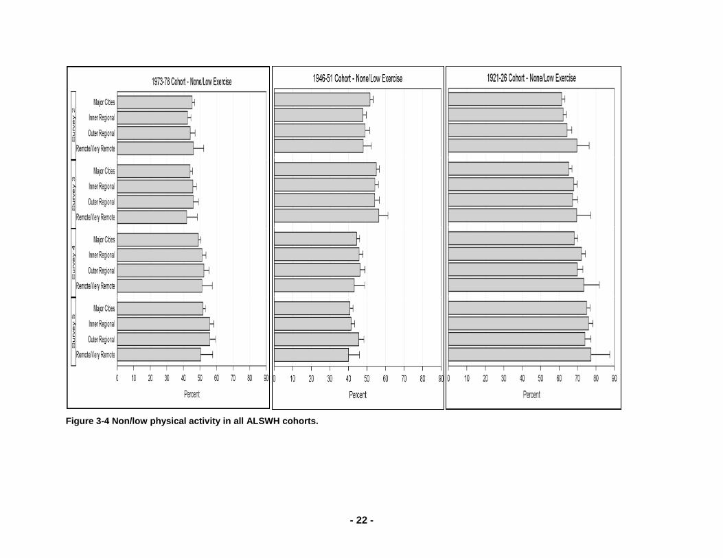
3.2.2. Chronic conditions
To illustrate the area differences and changes in chronic conditions over time, we present the data as bar
graphs showing the percentages of women in each area and cohort who reported that they had the
condition at Survey 1 (prevalent cases), the percentage of women who first reported the condition at
Surveys 2-5 (incident cases occurring between Surveys 1-5) and the percentage who never reported the
condition.
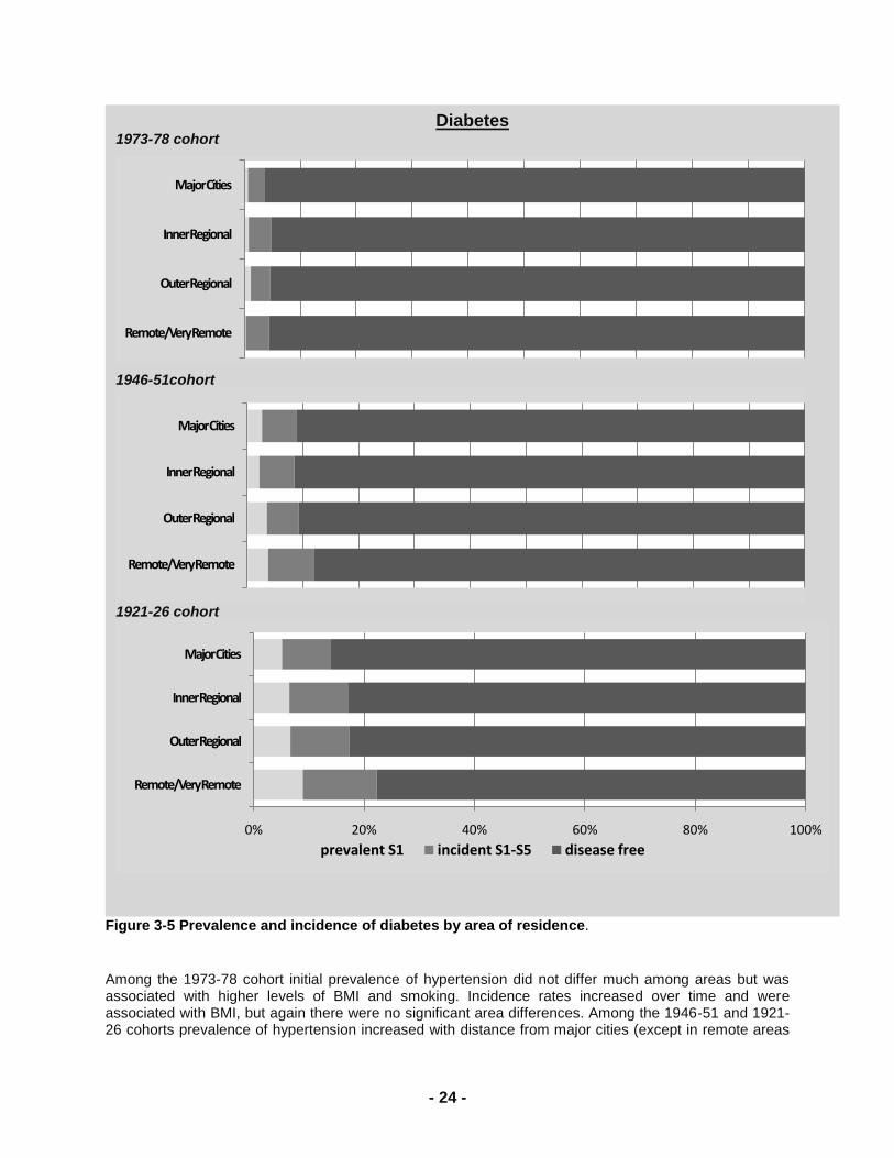
For diabetes, both prevalence and incidence were low for the 1973-78 cohort with little difference across
areas. Incidence increased across surveys and both prevalence and incidence were associated with
higher BMI.
For the 1946-51 and 1921-26 cohorts, prevalence and incidence of diabetes increased with distance from
major cities. For the mid-aged cohort prevalence and incidence were associated with higher BMI (and
with being born in Asia), and incidence increased over time. Differences in prevalence and incidence
across areas could be accounted for by differences in BMI. For the older women prevalence of diabetes
was strongly associated with BMI and being born in Asia; incidence rates increased over time but
differences among areas could be largely explained by BMI and differing levels of physical activity.
- 24 -
Figure 3-5 Prevalence and incidence of diabetes by area of residence.
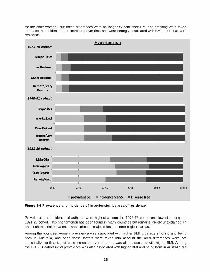
Among the 1973-78 cohort initial prevalence of hypertension did not differ much among areas but was associated with higher levels of BMI and smoking. Incidence rates increased over time and were associated with BMI, but again there were no significant area differences. Among the 1946-51 and 1921-26 cohorts prevalence of hypertension increased with distance from major cities (except in remote areas
Diabetes 1973-78 cohort
1946-51cohort
1921-26 cohort
Remote/Very Remote
Outer Regional
Inner Regional
Major Cities
Remote/Very Remote
Outer Regional
Inner Regional
Major Cities
0% 20% 40% 60% 80% 100%
Remote/Very Remote
Outer Regional
Inner Regional
Major Cities
prevalent S1 incident S1-S5 disease free
- 25 -
for the older women), but these differences were no longer evident once BMI and smoking were taken into account. Incidence rates increased over time and were strongly associated with BMI, but not area of residence.
Figure 3-6 Prevalence and incidence of hypertension by area of residence.
Prevalence and incidence of asthmas were highest among the 1973-78 cohort and lowest among the
1921-26 cohort. This phenomenon has been found in many countries but remains largely unexplained. In
each cohort initial prevalence was highest in major cities and inner regional areas.
Among the youngest women, prevalence was associated with higher BMI, cigarette smoking and being
born in Australia, and once these factors were taken into account the area differences were not
statistically significant. Incidence increased over time and was also associated with higher BMI. Among
the 1946-51 cohort initial prevalence was also associated with higher BMI and being born in Australia but
Hypertension 1973-78 cohort
1946-51 cohort
1921-26 cohort
Remote/Very Remote
Outer Regional
Inner Regional
Major Cities
Remote/Very Remote
Outer Regional
Inner Regional
Major Cities
0% 20% 40% 60% 80% 100%
Remote/Very …
Outer Regional
Inner Regional
Major Cities
prevalent S1 incidence S1-S5 Disease free
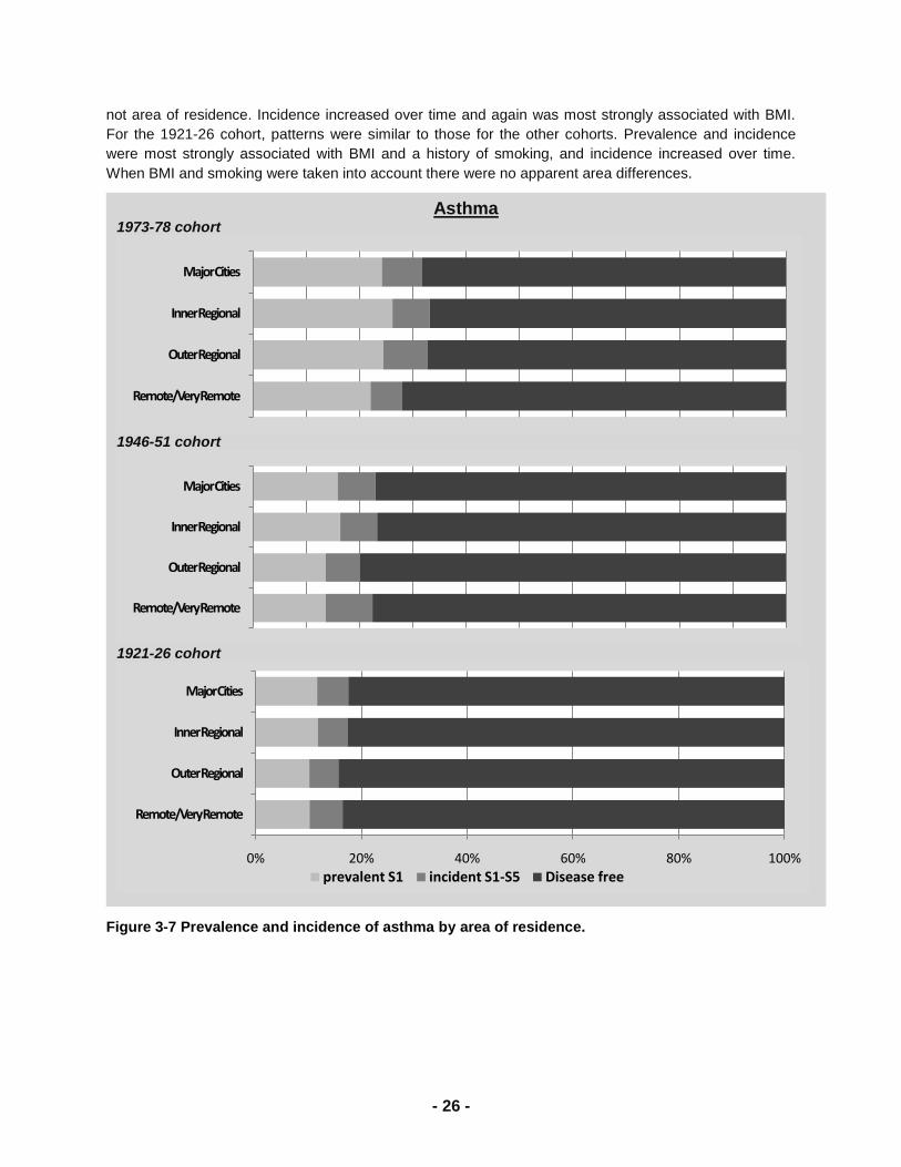
- 26 -
not area of residence. Incidence increased over time and again was most strongly associated with BMI.
For the 1921-26 cohort, patterns were similar to those for the other cohorts. Prevalence and incidence
were most strongly associated with BMI and a history of smoking, and incidence increased over time.
When BMI and smoking were taken into account there were no apparent area differences.
Figure 3-7 Prevalence and incidence of asthma by area of residence.
Asthma 1973-78 cohort
1946-51 cohort
1921-26 cohort
Remote/Very Remote
Outer Regional
Inner Regional
Major Cities
Remote/Very Remote
Outer Regional
Inner Regional
Major Cities
0% 20% 40% 60% 80% 100%
Remote/Very Remote
Outer Regional
Inner Regional
Major Cities
prevalent S1 incident S1-S5 Disease free
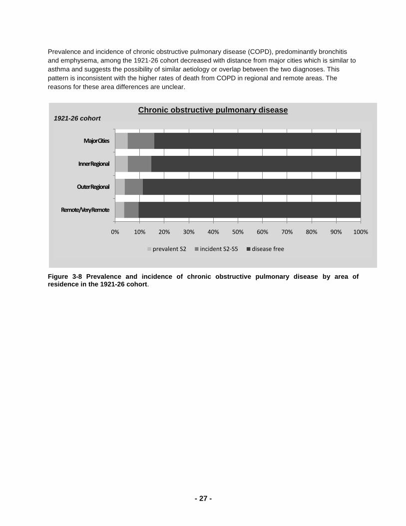
- 27 -
Prevalence and incidence of chronic obstructive pulmonary disease (COPD), predominantly bronchitis
and emphysema, among the 1921-26 cohort decreased with distance from major cities which is similar to
asthma and suggests the possibility of similar aetiology or overlap between the two diagnoses. This
pattern is inconsistent with the higher rates of death from COPD in regional and remote areas. The
reasons for these area differences are unclear.
Figure 3-8 Prevalence and incidence of chronic obstructive pulmonary disease by area of residence in the 1921-26 cohort.
Chronic obstructive pulmonary disease 1921-26 cohort
0% 10% 20% 30% 40% 50% 60% 70% 80% 90% 100%
Remote/Very Remote
Outer Regional
Inner Regional
Major Cities
prevalent S2 incident S2-S5 disease free
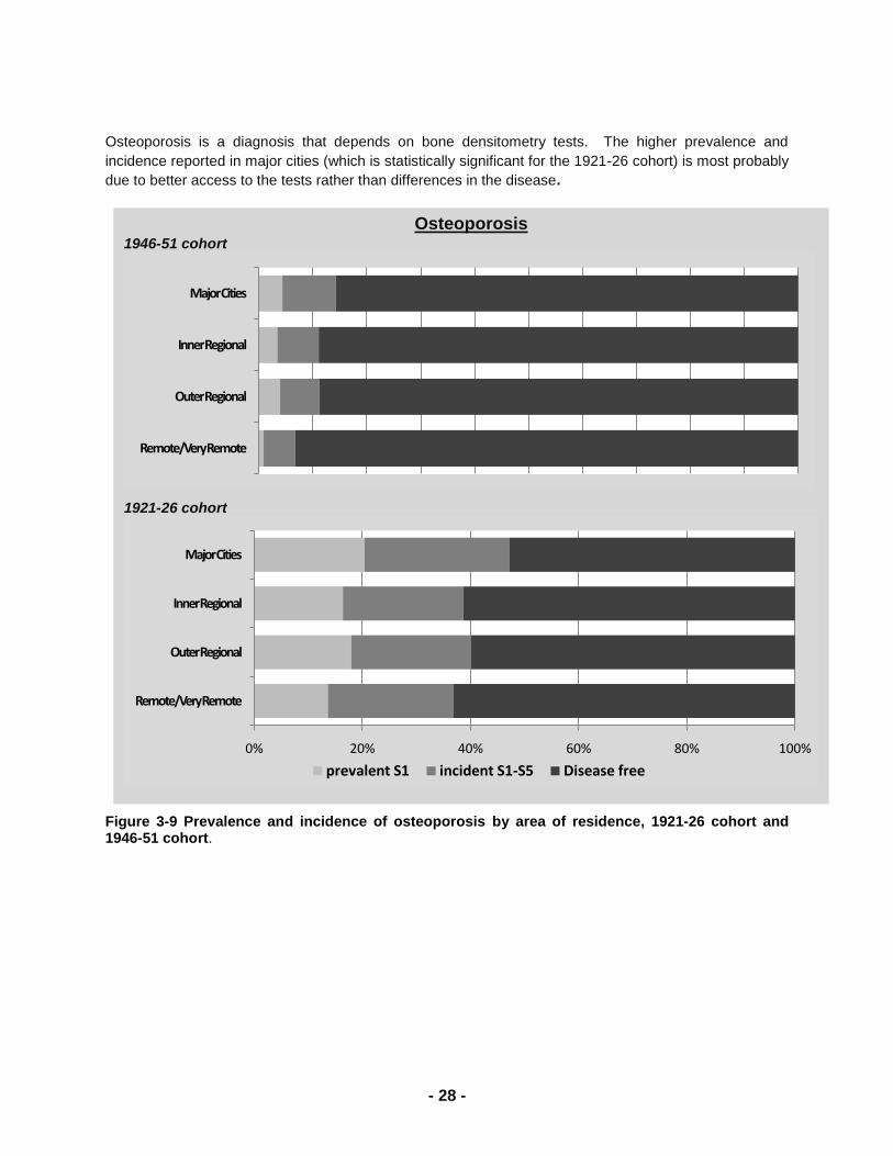
- 28 -
Osteoporosis is a diagnosis that depends on bone densitometry tests. The higher prevalence and
incidence reported in major cities (which is statistically significant for the 1921-26 cohort) is most probably
due to better access to the tests rather than differences in the disease.
Figure 3-9 Prevalence and incidence of osteoporosis by area of residence, 1921-26 cohort and 1946-51 cohort.
Osteoporosis 1946-51 cohort
1921-26 cohort
Remote/Very Remote
Outer Regional
Inner Regional
Major Cities
0% 20% 40% 60% 80% 100%
Remote/Very Remote
Outer Regional
Inner Regional
Major Cities
prevalent S1 incident S1-S5 Disease free
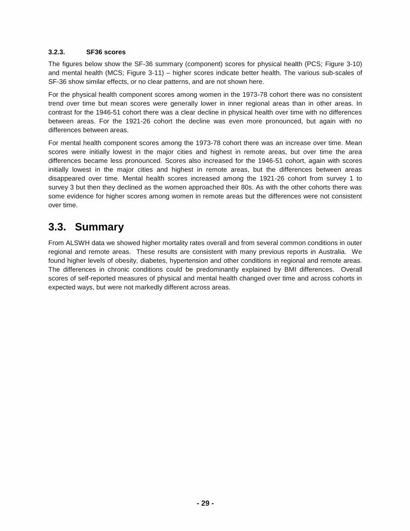
- 29 -
3.2.3. SF36 scores
The figures below show the SF-36 summary (component) scores for physical health (PCS; Figure 3-10)
and mental health (MCS; Figure 3-11) – higher scores indicate better health. The various sub-scales of
SF-36 show similar effects, or no clear patterns, and are not shown here.
For the physical health component scores among women in the 1973-78 cohort there was no consistent
trend over time but mean scores were generally lower in inner regional areas than in other areas. In
contrast for the 1946-51 cohort there was a clear decline in physical health over time with no differences
between areas. For the 1921-26 cohort the decline was even more pronounced, but again with no
differences between areas.
For mental health component scores among the 1973-78 cohort there was an increase over time. Mean
scores were initially lowest in the major cities and highest in remote areas, but over time the area
differences became less pronounced. Scores also increased for the 1946-51 cohort, again with scores
initially lowest in the major cities and highest in remote areas, but the differences between areas
disappeared over time. Mental health scores increased among the 1921-26 cohort from survey 1 to
survey 3 but then they declined as the women approached their 80s. As with the other cohorts there was
some evidence for higher scores among women in remote areas but the differences were not consistent
over time.
3.3. Summary
From ALSWH data we showed higher mortality rates overall and from several common conditions in outer
regional and remote areas. These results are consistent with many previous reports in Australia. We
found higher levels of obesity, diabetes, hypertension and other conditions in regional and remote areas.
The differences in chronic conditions could be predominantly explained by BMI differences. Overall
scores of self-reported measures of physical and mental health changed over time and across cohorts in
expected ways, but were not markedly different across areas.
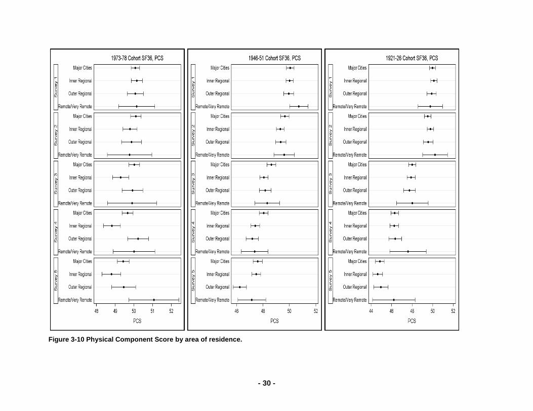
- 30 -
Figure 3-10 Physical Component Score by area of residence.
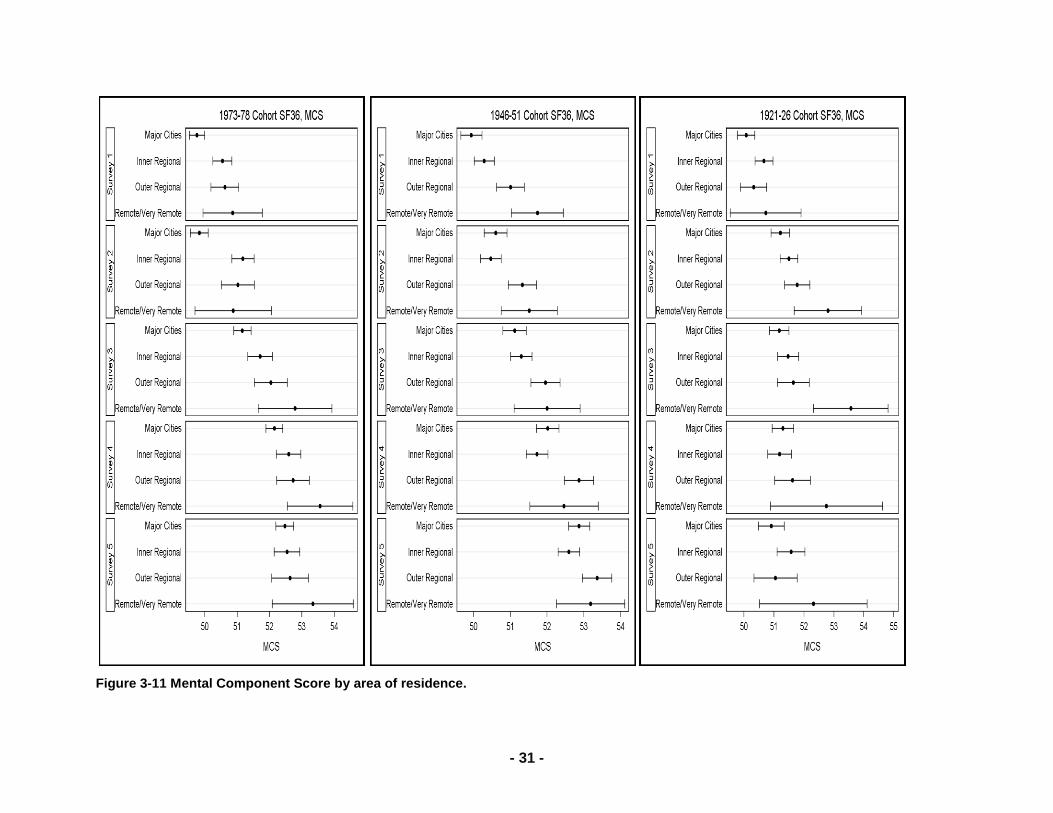
- 31 -
Figure 3-11 Mental Component Score by area of residence.
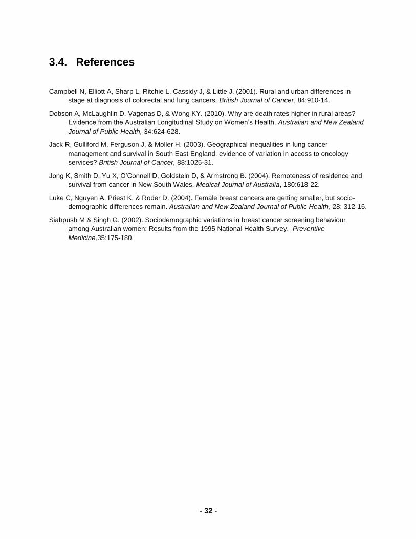
- 32 -
3.4. References
Campbell N, Elliott A, Sharp L, Ritchie L, Cassidy J, & Little J. (2001). Rural and urban differences in
stage at diagnosis of colorectal and lung cancers. British Journal of Cancer, 84:910-14.
Dobson A, McLaughlin D, Vagenas D, & Wong KY. (2010). Why are death rates higher in rural areas?
Evidence from the Australian Longitudinal Study on Women‘s Health. Australian and New Zealand
Journal of Public Health, 34:624-628.
Jack R, Gulliford M, Ferguson J, & Moller H. (2003). Geographical inequalities in lung cancer
management and survival in South East England: evidence of variation in access to oncology
services? British Journal of Cancer, 88:1025-31.
Jong K, Smith D, Yu X, O‘Connell D, Goldstein D, & Armstrong B. (2004). Remoteness of residence and
survival from cancer in New South Wales. Medical Journal of Australia, 180:618-22.
Luke C, Nguyen A, Priest K, & Roder D. (2004). Female breast cancers are getting smaller, but socio-
demographic differences remain. Australian and New Zealand Journal of Public Health, 28: 312-16.
Siahpush M & Singh G. (2002). Sociodemographic variations in breast cancer screening behaviour
among Australian women: Results from the 1995 National Health Survey. Preventive
Medicine,35:175-180.
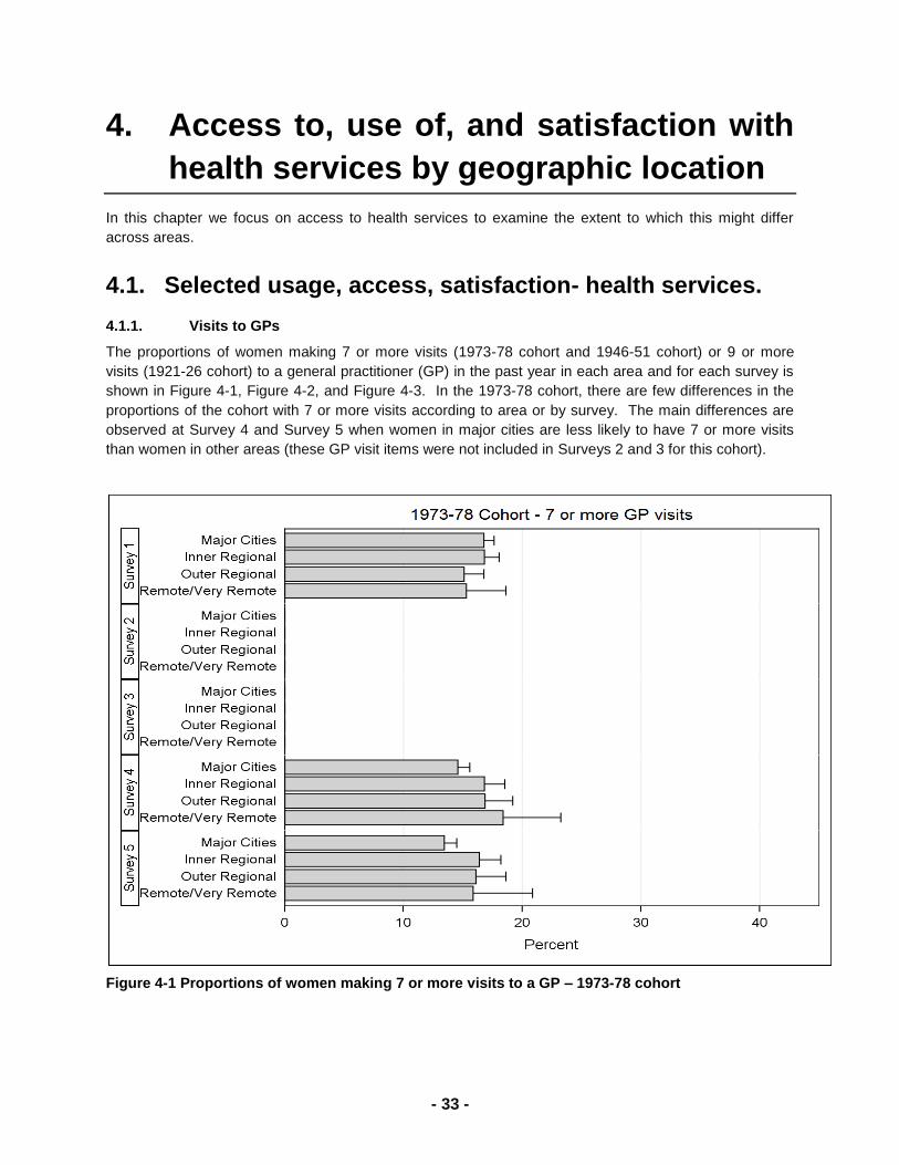
- 33 -
4. Access to, use of, and satisfaction with
health services by geographic location
In this chapter we focus on access to health services to examine the extent to which this might differ
across areas.
4.1. Selected usage, access, satisfaction- health services.
4.1.1. Visits to GPs
The proportions of women making 7 or more visits (1973-78 cohort and 1946-51 cohort) or 9 or more
visits (1921-26 cohort) to a general practitioner (GP) in the past year in each area and for each survey is
shown in Figure 4-1, Figure 4-2, and Figure 4-3. In the 1973-78 cohort, there are few differences in the
proportions of the cohort with 7 or more visits according to area or by survey. The main differences are
observed at Survey 4 and Survey 5 when women in major cities are less likely to have 7 or more visits
than women in other areas (these GP visit items were not included in Surveys 2 and 3 for this cohort).
Figure 4-1 Proportions of women making 7 or more visits to a GP – 1973-78 cohort
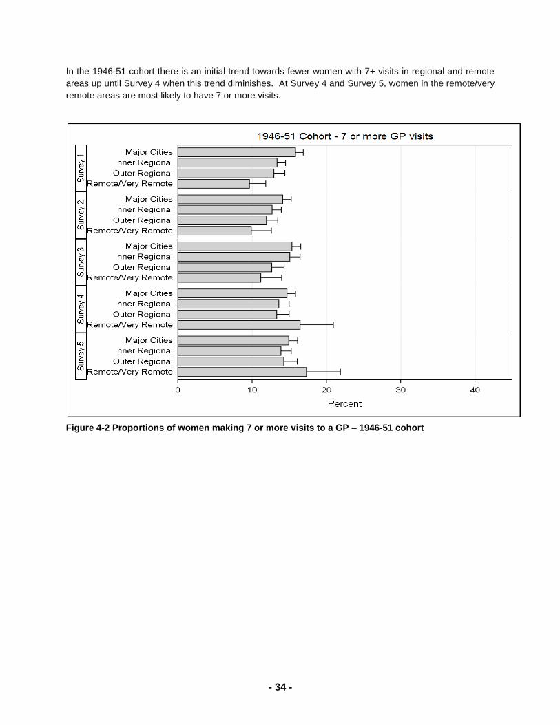
- 34 -
In the 1946-51 cohort there is an initial trend towards fewer women with 7+ visits in regional and remote
areas up until Survey 4 when this trend diminishes. At Survey 4 and Survey 5, women in the remote/very
remote areas are most likely to have 7 or more visits.
Figure 4-2 Proportions of women making 7 or more visits to a GP – 1946-51 cohort
- 35 -
The cut-point of 9 or more GP visits was applied for older women in recognition of the higher overall rate
of GP use among this age group. In this cohort, there is a clear difference between major cities and other
areas, with women in major cities being much more likely to have had nine or more visits per year.
Figure 4-3 Proportions of women making 7 or more visits to a GP – 1921-26 cohort
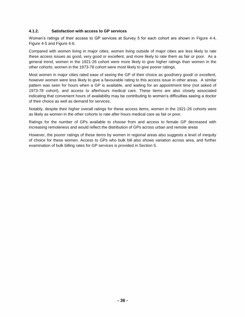
- 36 -
4.1.2. Satisfaction with access to GP services
Women‘s ratings of their access to GP services at Survey 5 for each cohort are shown in Figure 4-4,
Figure 4-5 and Figure 4-6.
Compared with women living in major cities, women living outside of major cities are less likely to rate
these access issues as good, very good or excellent, and more likely to rate them as fair or poor. As a
general trend, women in the 1921-26 cohort were more likely to give higher ratings than women in the
other cohorts; women in the 1973-78 cohort were most likely to give poorer ratings.
Most women in major cities rated ease of seeing the GP of their choice as good/very good/ or excellent,
however women were less likely to give a favourable rating to this access issue in other areas. A similar
pattern was seen for hours when a GP is available, and waiting for an appointment time (not asked of
1973-78 cohort), and access to afterhours medical care. These items are also closely associated
indicating that convenient hours of availability may be contributing to women‘s difficulties seeing a doctor
of their choice as well as demand for services.
Notably, despite their higher overall ratings for these access items, women in the 1921-26 cohorts were
as likely as women in the other cohorts to rate after hours medical care as fair or poor.
Ratings for the number of GPs available to choose from and access to female GP decreased with
increasing remoteness and would reflect the distribution of GPs across urban and remote areas
However, the poorer ratings of these items by women in regional areas also suggests a level of inequity
of choice for these women. Access to GPs who bulk bill also shows variation across area, and further
examination of bulk billing rates for GP services is provided in Section 5.
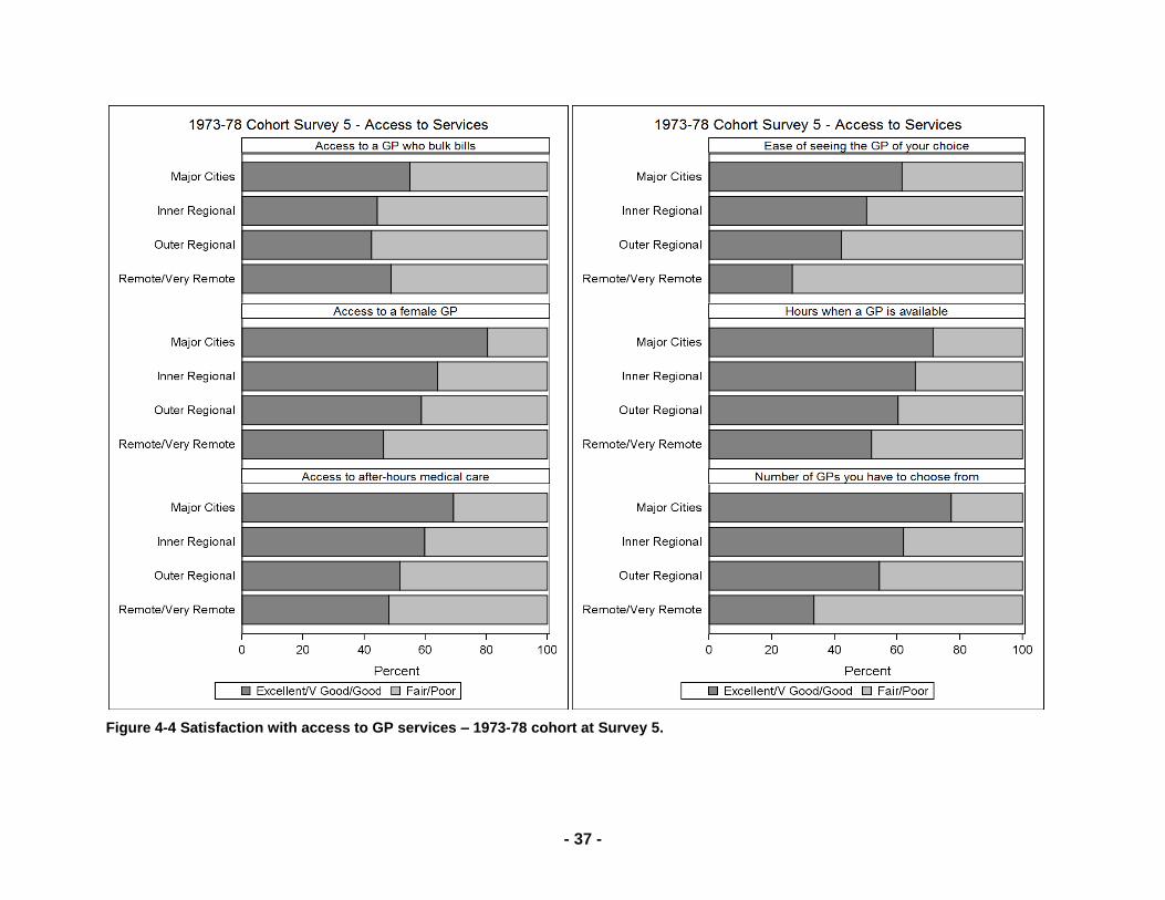
- 37 -
Figure 4-4 Satisfaction with access to GP services – 1973-78 cohort at Survey 5.
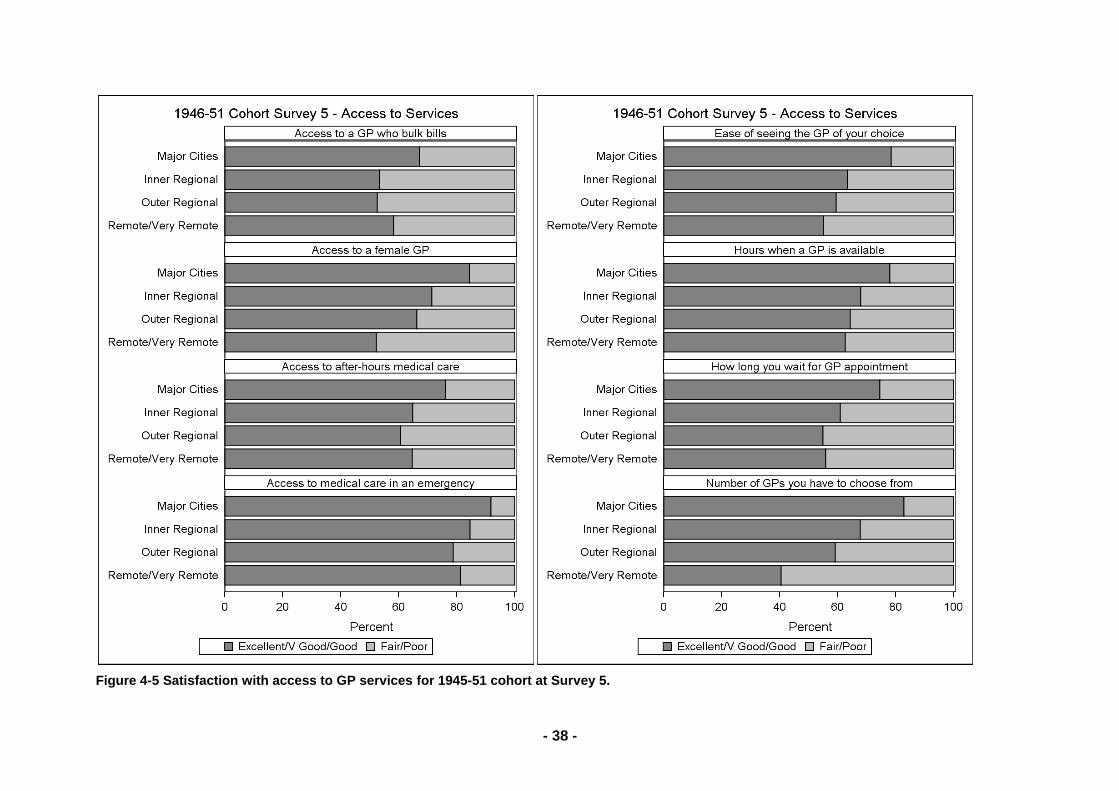
- 38 -
Figure 4-5 Satisfaction with access to GP services for 1945-51 cohort at Survey 5.
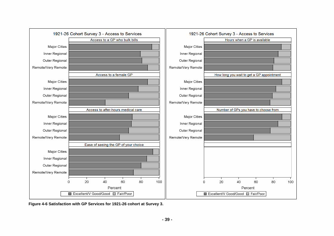
- 39 -
Figure 4-6 Satisfaction with GP Services for 1921-26 cohort at Survey 3.
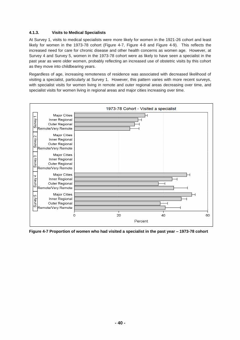
- 40 -
4.1.3. Visits to Medical Specialists
At Survey 1, visits to medical specialists were more likely for women in the 1921-26 cohort and least
likely for women in the 1973-78 cohort (Figure 4-7, Figure 4-8 and Figure 4-9). This reflects the
increased need for care for chronic disease and other health concerns as women age. However, at
Survey 4 and Survey 5, women in the 1973-78 cohort were as likely to have seen a specialist in the
past year as were older women, probably reflecting an increased use of obstetric visits by this cohort
as they move into childbearing years.
Regardless of age, increasing remoteness of residence was associated with decreased likelihood of
visiting a specialist, particularly at Survey 1. However, this pattern varies with more recent surveys,
with specialist visits for women living in remote and outer regional areas decreasing over time, and
specialist visits for women living in regional areas and major cities increasing over time.
Figure 4-7 Proportion of women who had visited a specialist in the past year – 1973-78 cohort
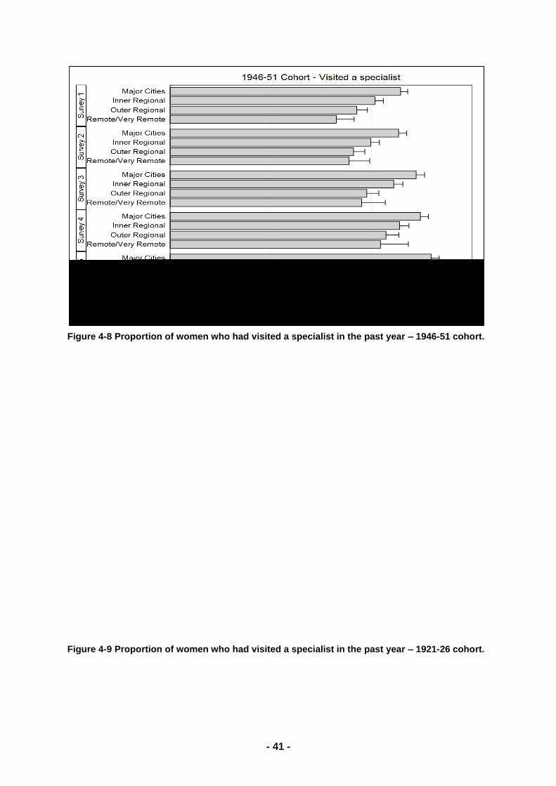
- 41 -
Figure 4-8 Proportion of women who had visited a specialist in the past year – 1946-51 cohort.
Figure 4-9 Proportion of women who had visited a specialist in the past year – 1921-26 cohort.

- 60 -
Poor oral health carries a high burden of illness, particularly among older people, but preventative and
treatment dentistry can significantly reduce this burden (Chalmers, 2003). However, access to dental
care may present a barrier for non-urban residents in obtaining dental care (Slack-Smith & Hyndman,
2004). A study of older Western Australians identified that visits to a dentist are lower for those
residing in non-urban areas (44%) compared to urban areas (65%) (Adams et al., 2004). Other
factors influencing higher levels of dental service utilisation among older adults are higher levels of
income (Osterberg et al., 1998) and education (Slack-Smith & Hyndman, 2004; Osterberg et al.,
1998), being female (Adams et al., 2004), married or defacto (Osterberg et al., 1998), having private
health insurance (Slack-Smith & Hyndman, 2004), non-smokers and those with higher levels of
physical activity (Slack-Smith & Hyndman, 2004; Osterberg et al., 1998).
Detailed analysis of data from the second survey of ALSWH, involving 10,433 women aged 73-78
years in 1999, show that 35% of these women had consulted a dentist at least once in the previous
12 months (after correcting for over-sampling in rural and remote areas) (Cockerell et al., 2007).
Women were less likely to visit a dentist if they live in a non-urban area, were born in Australia, had
less education, and were separated, widowed or divorced (Figure 4-3). Women were more likely to
visit a dentist if they had private ancillary insurance. Women who had at least one chronic illness were
less likely to visit a dentist, but women who had more symptoms and those who reported that they
take medications for a long-term illness, HRT and/or non-prescription medications were more likely to
visit a dentist. Visits to dentists were also positively associated with eating fruits/vegetables most
days, and with higher scores on the Physical Functioning sub-scale.

- 61 -
Table 4-3 Adjusted† odds ratios and associated 95% confidence intervals (C.I.) for factors associated with visits to a dentist by older women
Characteristic Odds Ratio 95% C.I.
Area urban 1.00 —
non-urban 0.77 (0.67, 0.88)
Education no formal 1.00 —
high school 2.16 (1.82, 2.57)
trade/certif./dip. 2.66 (2.12, 3.34)
university 4.12 (2.98, 5.79)
Marital status married/defacto 1.00 —
sep./div./widow. 0.79 (0.68, 0.90)
single 1.03 (0.71, 1.50)
Country of birth Australia 1.00 —
Other ESB 1.40 (1.15, 1.70)
Europe 1.37 (1.05, 1.80)
Asia 2.04 (1.06, 3.92)
other 1.60 (0.73, 3.51)
Insurance no 1.00 —
yes 2.59 (2.25, 2.97)
Chronic illness no 1.00 —
yes 0.74 (0.62, 0.88)
Medications for no 1.00 —
long-term illness yes 1.28 (1.08, 1.51)
Medications for no 1.00 —
Hormone Replacement Therapy (HRT)
yes 1.40 (1.14, 1.72)
Non-prescription no 1.00 —
medications yes 1.33 (1.14, 1.54)
Eat fruit or false 1.00 —
vegetables true 2.81 (1.38, 5.68)
SF-36 physical functioning
(5pt increase)
1.05 (1.03, 1.07)
No. of symptoms 1.04 (1.02, 1.07)
† The multivariate logistic regression model was obtained using a backward stepwise approach.

- 62 -
Further analysis using longitudinal data from Surveys 2, 3 and 4 shows the percentages of women
who consulted a dentist in the years 1999, 2002 and 2005 were 35%, 36% and 37% respectively
(Sibbritt et al., 2010). There were 6,170 women who answered the question related to consultation
with a dentist at all three survey points. Of these women: 22% reported consulting a dentist on all 3
surveys; 15% reported consulting a dentist on 2 of the surveys; and 19% reported consulting a dentist
on only 1 of the surveys.
In Survey 4, there were 325 (5%) women who needed to see a dentist but did not consult one. The
reasons given for not consulting a dentist by these women were (they could indicate more than one
reason): there was no dentist available locally (n=58); travel difficulties, I could not get there (n=81);
long waiting period for an appointment (n=158); I could not afford to see a dentist (n=156).
Longitudinal analysis of factors associated with consulting a dentist shows that women who live in
urban areas were 1.47 (95% CI: 1.36, 1.58) times more likely to consult with a dentist than women
who live in rural areas. In comparison to women who were married or in a de facto relationship,
women who were separated, divorced or widowed were 0.87 (95% CI: 0.81, 0.93) times less likely to
consult with a dentist. Non-smoking women were 1.61 (95% CI: 1.34, 1.94) times more likely to
consult with a dentist. In comparison to women who find it easy to live on their income, women who
find it difficult to live on their income some of the time were 0.83 (95% CI: 075, 0.91) times less likely
to consult with a dentist (see Table 4-4). Women who find it impossible or difficult to live on their
income all of the time were also less likely to consult with a dentist (OR= 0.90; 95% CI: 078, 1.03), but
this was not statistically significant, possible because of the small number of women who are in this
category. In comparison to women with a university education, women with a trade, certificate or
diploma (OR=0.60; 95% CI: 0.49, 0.74), high school education (OR=0.43; 95% CI: 0.36, 0.52), or no
formal education (OR=0.25; 95% CI: 0.21, 0.31) were all less likely to consult with a dentist. Women
who do not have diabetes were 1.25 (95% CI: 1.12, 1.40) times more likely to consult with a dentist,
as were women who do not have heart disease who are 1.13 (95% CI: 1.04, 1.24) times more likely to
consult with a dentist. Women who did not require home maintenance service were 0.81 (95% CI:
0.76, 0.86) times less likely to consult with a dentist. In terms of the SF-36 physical functioning score,
for every 5 point increase, women were 1.02 (95% CI: 1.01, 1.03) times more likely to consult with a
dentist.

- 63 -
Table 4-4 Factors associated with dentist consultations by older Australian women, derived from a longitudinal analysis using multivariable generalized estimation equation(GEE) modelling with backward stepwise elimination (n=9,387)
Factors OR 95% C.I. p-value
Area of residence urban 1.467 1.362, 1.579 <0.0001
(reference) rural 1 ―
Marital status never married 1.333 1.060, 1.677 0.0140
separated, divorced, widowed 0.865 0.806, 0.929 <0.0001
(reference) married, defacto 1 ―
Smoking status non-smoker 1.611 1.337, 1.941 <0.0001
(reference) smoker 1 ―
Ability to manage on impossible/difficult all the time 0.896 0.778, 1.033 0.1315
Income difficult some of the time 0.828 0.753, 0.911 <0.0001
it is not too bad 0.918 0.856, 0.985 0.017
(reference) it is easy 1 ―
Education level no formal 0.252 0.207, 0.305 <0.0001
High school 0.430 0.357, 0.519 <0.0001
trade, certificate, diploma 0.597 0.486, 0.735 <0.0001
(reference) university 1 ―
Diabetes status no 1.253 1.123, 1.399 <0.0001
(reference) yes 1 ―
Heart disease no 1.134 1.037, 1.240 0.0061
Status (reference) yes 1 ―
Required home no 0.809 0.759, 0.862 <0.0001
maintenance services (reference) yes 1 ―
SF36-physical functioning
(5 point increase) 1.022 1.014, 1.028 <0.0001

- 64 -
4.3.1. Discussion
Oral health is fundamental to overall health and quality of life, at all ages. Data from ALSWH identify a
large unmet need for dental care and a significant opportunity for public health intervention. Access
to dental care, in terms of location of dentists and affordability, contribute significantly to visits to a
dentist. In addition, having good nutrition, being married, and having a number of symptoms were also
associated with increased likelihood of visits to a dentist.
Oral health problems are of particular importance for older people and are among the most common
problems affecting their health (Chalmers, 2003). These problems can lead to impaired nutrition,
systemic disease, speech problems, and social withdrawal (Chalmers, 2003; Slack-Smith &
Hyndman, 2004). However many oral health problems can be prevented or treated by dental care.
This study has identified the under-use of dental services by certain socioeconomic groups that may
highlight a major source of health inequity in the community.
There has been a separation of dentistry away from medicine, with the Australian Government
providing substantial funding for services provided by doctors and hospitals, but not for dental
services (Lewis, 2008). Recent work by the Australian Institute of Health and Welfare reports that the
total contribution of all levels of government to medical and hospital expenditure was 78% and 81%
respectively, compared with 21% for dental services (AIHW, 2006). Under this system many
Australians are faced with paying substantial out-of-pocket costs for private care, or waiting up to two
years to access care through the public dental system (NHHRC, 2009). More recently, oral health
care has been identified as one of the top priorities by the Health and Hospitals Reform Commission
(NHHRC, 2009).
The implications of the poor utilisation of oral health care by older women are substantial. Good oral
health is an integral component of good general health (Williams et al., 2008; Kandelman, Peterson &
Ueda, 2008) at all ages. Clearly, there are physical health benefits to good oral health where losing
dental health affects one‘s food preference, resulting in poor nutrition and an associated increased
risk of disease (Arai et al., 2003). There are also mental health benefits to good oral health. If a
person‘s food choices are restricted then it takes away their enjoyment of eating (Arai et al., 2003).
Further, in a social context, the condition of a person‘s mouth and teeth can have a significant affect
on their self-esteem (McKenzie-Green et al., 2009).

- 65 -
4.3.2. References
Adams C, Slack-Smith L, Larson A, O'Grady M. Dentist visits in older Western Australians: A
comparison of urban, rural and remote residents. Australian Journal of Rural Health
2004;12:143-149.
Australian Institute of Health and Welfare (AIHW). Australia’s Health 2006, Australian Institute of
Health and Welfare, Canberra, 2006.
Arai K, Sumi Y, Uematsu H, Miura H. Association between dental health behaviours, mental/physical
function and self-feeding ability among the elderly: a cross-sectional survey. Gerontology 2003;
20(2):78-83.
Chalmers JM. Oral Health Promotion for our ageing Australian population. Australian Dental Journal
2003;48(1):2-9.
Cockrell D, Sibbritt D, Byles J. The prevalence and characteristics of older Australian women who
consult dentists. Australian Journal of Rural Health, 2007:15(6):387-388
Kandelman D, Petersen PE, Ueda H. Oral health, general health, and quality of life in older people.
Special Care in Dentistry 2008; 28(6): 224-236.
Lewis JM. The road to oral health policy innovation in Australia. Australian Review of Public Affairs,
2007. Electronic resource: http://www.australianreview.net/digest/2007/election/lewis.html
(access 25 October 2008).
National Health and Hospitals Reform Commission. 2009. A Healthier Future for all Australians –
Final Report of the National Health and Hospitals Reform Commission.
CommonwealthGovernment of Australia. ISBN: 1-74186-940-4
http://www.health.gov.au/internet/nhhrc/publishing.nsf/Content/nhhrc-report
Osterberg T, Lundgren M, Emilson CG, Sundh V, & Birkhed D, B S. Utilization of dental services in
relation to socioeconomic and health factors in the middle-aged and elderly Swedish
population. Acta Odontologica Scandinavica 1998;56(1):41-7.
Slack-Smith L, & Hyndman J. The relationship between demographic and health-related factors on
dental service attendance by older Australians. British Dental Journal 2004;197(4):193-199.
Sibbritt DW, Byles JE, & Tavener M. Older Australian women‘s use of dentists: a longitudinal analysis
over 6 years. Australasian Journal of Ageing 2010;29(1):14-20.
Williams RC, Barnett AH, Claffey N, Davis M, Gadsby R, Kellet M, Lip GYH, & Thackray S. The
potential impact of periodontal disease on general health: a consensus view. Current Medical
Research and Opinions 2008; 24(6): 1635-1643.

- 66 -
4.4. Complementary and alternative medicine (CAM)
Note that the source for the first part of this section is from published work:
Source: Jon Adams, David Sibbritt, Chi-Wai Lui. The Urban-Rural Divide in Complementary and
Alternative Medicine Use: A Longitudinal Study of 10,638 Women. BMC Complementary & Alternative Medicine (accepted November, 2010)
4.4.1. Introduction
Complementary and alternative medicine (CAM) refers to those practices, technologies and
medications not traditionally part of conventional care and includes acupuncture, aromatherapy,
chiropractic, homeopathy, reflexology, massage therapy and osteopathy, among others. The use of
CAM has achieved mainstream status in Western countries over past decades (Barnes et al., 2008;
Hanssen et al., 2005) and surveys on patterns of CAM use reveal that such health seeking behaviour
is not confined to metropolitan settings. There is evidence that residents in rural and remote regions
also employ a variety of treatments to complement their conventional care and to manage chronic
health problems like diabetes and arthritis (Kirkpatrick et al., 2006; Wilkinson & Jelinek, 2009;
Shreffler-Grant et al., 2005). Previous surveys of patients from rural community centers or health
clinics suggest prevalence rates for CAM use ranging from between 39% and 87% (Kirkpatrick et al.,
2006; Wilkinson & Jelinek, 2009). CAM is also found to be used by older rural adults as a common
strategy for maintaining health and wellbeing (as distinct from treating specific health problems and
conditions) (Wilkinson & Jelinek, 2009; Shreffler-Grant et al., 2007). A longitudinal analysis of ALSWH
data collected from the 1946-51 cohort also suggested that CAM consumption is higher in non-urban
regions than in urban areas (Adams et al., 2003; Sibbritt et al., 2004).
Of the 10,638 women who completed the 1946-51 cohort Survey 5, 40% were living in urban areas,
56% in rural areas and 4% in remote areas. Among these women, 30% had consulted a CAM
practitioner in the previous 12 months. The percentage of women who consulted a CAM practitioner
varied by place of residence: 28%, 32% and 30% for urban, rural and remote areas respectively.
4.4.2. Consultations with conventional health care providers by CAM use
Table 4-5 shows that overall, CAM users tend to consult with a GP more frequently than CAM non-
users. This pattern can be seen separately for the three areas of residence, although the association
is only statistically significant for urban and rural areas. Similarly, CAM users tend to consult with a
specialist doctor more frequently than CAM non-users within the three areas of residence and overall.
There is no statistically significant association between CAM user status and consultation with a
hospital doctor overall or within the three areas of residence.

- 67 -
Table 4-5 Consultations with conventional health care providers by CAM use (consulted with a CAM practitioner or not)
Urban Rural Remote
CAM
non-user CAM user CAM non-
user CAM user CAM non-
user CAM user
Consultations
(n = 2960)
%
(n = 1157)
%
(n = 4011)
%
(n = 1866)
%
(n = 308)
%
(n = 131)
%
GP ■ 1 2
0 6 5 7 5 9 8
1-2 34 27 36 32 36 31
3-4 31 32 29 28 28 32
5-6 16 17 15 18 14 16
7-12 9 13 9 11 9 10
13+ 4 6 4 6 4 3
Hospital Doctor
0 83 80 82 80 80 76
1-2 13 15 15 16 14 19
3+ 4 5 3 4 6 5
Specialist Doctor
■ 1 2 3
0 51 44 57 52 63 48
1-2 32 34 30 32 25 39
3-4 11 13 8 10 8 8
5-6 3 5 3 3 1 1
7+ 3 4 2 3 3 4
Note: chi-square tests used to test for statistically significant associations. ■ Statistically significant association for CAM user status (i.e. ignoring place of residence) (P < .005)
1 Statistically significant association for urban residents (P < .005)
2 Statistically significant association for rural residents (P < .005)
3 Statistically significant association for remote residents (P < .05)
Source: Jon Adams, David Sibbritt, Chi-Wai Lui. The Urban-Rural Divide in Complementary and Alternative
Medicine Use: A Longitudinal Study of 10,638 Women. BMC Complementary & Alternative Medicine (accepted
November, 2010)
4.4.3. Rating of conventional health care providers by CAM use
The relationship between the ratings of various aspects of conventional health care provision and
CAM user status is shown in Table 4-6. In general, CAM users were more dissatisfied with the
outcomes of their medical care than CAM non-users. This was a consistent pattern across the three
areas of residence, although it was not statistically significant for women from remote areas.
Furthermore, CAM users were more dissatisfied with the hours when a GP was available, the ease of
seeing a GP of their choice, and the waiting time to get a GP appointment than CAM non-users.
There were consistent patterns across the three areas of residence for all of these aspects, although
they were only statistically significant for women from urban areas. CAM users in urban areas only
were also more dissatisfied with access to a medical specialist if needed compared to CAM non-
users. There were no statistically significant associations, either overall or separate areas of
residence, between CAM user status and access to a female GP.

- 68 -
Table 4-6 Rating of conventional health care providers by CAM use (consulted with a CAM practitioner or not) Level of Satisfaction (1=excellent … 5=poor).
Urban Rural Remote
CAM
non-user
CAM
user
CAM
non-user
CAM
user
CAM
non-user
CAM
user
(n = 2960)
(n = 1157)
(n = 4011)
(n = 1866)
(n = 308) (n = 131)
mean mean mean mean mean mean
Access to a medical specialist if needed
1
1.93 2.02 2.50 2.48 3.11 3.14
Access to a female GP 2.24 2.30 2.76 2.74 3.39 3.44
Hours when a GP is available
■ 1
2.65 2.80 2.90 2.97 3.22 3.34
Number of GPs you have to choose from
■ 1
2.50 2.62 2.94 2.97 3.67 3.67
Ease of seeing GP of your choice
■ 1
2.58 2.75 2.97 3.04 3.32 3.50
How long you wait to get a GP appointment
■
1
2.74 2.87 3.12 3.18 3.35 3.54
The outcomes of your medical care
■ 1 2
(how much you are helped)
2.27 2.41 2.45 2.54 2.67 2.81
Note: Student t-tests used to test for statistically significant differences. ■ Statistically significant association for CAM user status (i.e. ignoring place of residence) (P < .005)
1 Statistically significant association for urban residents (P < .005)
2 Statistically significant association for rural residents (P < .005)
3 Statistically significant association for remote residents (P < .05)
Source: Jon Adams, David Sibbritt, Chi-Wai Lui. The Urban-Rural Divide in Complementary and Alternative
Medicine Use: A Longitudinal Study of 10,638 Women. BMC Complementary & Alternative Medicine (accepted
November, 2010)
4.4.4. Symptoms and diagnoses by CAM use
Table 4-7 shows the association between the symptoms that women sought help for and
consultations with a CAM practitioner. Overall, CAM users were significantly more likely than non-
CAM users to seek help for severe tiredness. This was a consistent pattern across all the three areas
of residence, although it was only statistically significant for women from rural and remote areas. CAM
users were also significantly more likely than non-users to seek help for night sweats and anxiety.
There were consistent patterns across the three areas of residence for these two aspects, although
they were only statistically significant for women from rural areas. A greater percentage of CAM users
sought help for depression across the three areas of residence, but this was only statistically
significant for women from remote areas. The analysis also demonstrates that CAM users were
significantly more likely to seek help for back pain. This was a consistent and statistically significant
pattern across the three areas of residence. In addition, CAM users were significantly more likely to
seek help for indigestion or heartburn, headaches or migraines, stiff or painful joints, urine that burns
or stings, hot flushes. There were consistent patterns across the three areas of residence for all of
these aspects, although they were only statistically significant for women from urban and rural areas.
Finally, CAM users were significantly more likely than non-CAM users to seek help for allergies or
hayfever or sinusitis. This was a consistent and statistically significant pattern across the three areas

- 69 -
of residence, although it was only statistically significant for women from urban areas. There were no
statistically significant associations between CAM user status and breathing difficulties or chest pain.
Table 4-7 Sought help for symptoms by CAM use (consulted with a CAM practitioner or not)
Urban Rural Remote
Sought help for the following symptoms:
CAM
non-user
CAM
user
CAM
non-user
CAM
user
CAM
non-user
CAM
user
(n = 2960) (n = 1157) (n = 4011) (n = 1866) (n = 308) (n = 131)
Allergies, hayfever, sinusitis
■ 1
% yes 13 19 13 16 13 16
Breathing difficulties
% yes 7 9 8 9 7 6
Indigestion or heartburn
■ 1 2
% yes 9 13 9 13 10 11
Chest pain % yes 6 7 6 6 6 8
Headaches or migraines
■ 1 2
% yes 6 9 7 10 6 9
Severe tiredness
■ 2 3
% yes 6 8 6 9 5 10
Stiff or painful joints
■ 1 2
% yes 15 26 18 25 15 18
Back pain ■ 1 2 3
% yes 12 31 12 29 11 29
Urine that burns or stings ■ 1 2
% yes 4 7 4 7 6 3
Hot flushes ■ 1 2
% yes 6 10 6 10 5 5
Night sweats ■ 2
% yes 5 7 4 7 4 5
Depression 3 % yes 8 9 8 9 4 9
Anxiety ■ 2
% yes 7 9 6 9 4 6
Note: chi-square tests used to test for statistically significant associations. ■ Statistically significant association for CAM user status (i.e. ignoring place of residence) (P < .005)
1 Statistically significant association for urban residents (P < .005)
2 Statistically significant association for rural residents (P < .005)
3 Statistically significant association for remote residents (P < .05)
Source: Jon Adams, David Sibbritt, Chi-Wai Lui. The Urban-Rural Divide in Complementary and
Alternative Medicine Use: A Longitudinal Study of 10,638 Women. BMC Complementary & Alternative
Medicine (accepted November, 2010)
4.4.5. Diseases and consultations with a CAM practitioner
Table 4-8 shows the association between the diseases that women have been diagnosed with and
consultations with a CAM practitioner. Overall, CAM users were more likely than non-CAM users to
report osteoporosis. This was a consistent, statistically significant pattern across the three areas of
residence. CAM users are also more likely to have asthma and bronchitis/emphysema. There were
consistent patterns across the three areas of residence for these two diagnoses, although they were
not statistically significant for the separate areas of residence. The analysis shows that CAM users
are more likely to report arthritis. This was a consistent pattern across the three areas of residence,
although it was only statistically significant for women from urban and rural areas. CAM users are also

- 70 -
more likely to report low iron levels. This was a consistent pattern across the three areas of residence,
although it was only statistically significant for women from urban areas. In addition, CAM users are
more likely to report hypertension. This was a consistent pattern across the three areas of residence,
although it was only statistically significant for women from rural areas. Finally, CAM users are more
likely to report skin cancer. This was a consistent pattern across the three areas of residence,
although it was only statistically significant for women from remote areas. For all other cancers and for
diabetes and heart disease there were no statistically significant associations with CAM user status.
Table 4-8 Diagnoses by CAM user status (consulted with a CAM practitioner or not)
Urban Rural Remote
Diagnoses
CAM
non-user
CAM
user
CAM
non-user
CAM
user
CAM
non-user
CAM
user
(n = 2960) (n = 1157) (n = 4011) (n = 1866) (n = 308) (n = 131)
Diabetes % yes 26 26 27 26 31 24
Arthritis ■ 1 2
% yes 34 40 35 41 33 36
Heart Disease
% yes 6 6 7 7 8 7
Hypertension
■ 2
% yes 32 32 38 33 41 32
Low iron level
■ 1
% yes 30 36 28 32 26 34
Asthma ■ % yes 19 21 19 21 18 20
Bronchitis/emphysema
■
% yes 18 20 17 19 13 18
Osteoporosis
■ 1 2 3
% yes 11 15 9 11 5 11
Breast cancer
% yes 5 6 5 5 3 4
Cervical cancer
% yes 3 3 3 3 2 2
Skin cancer ■ 3
% yes 20 21 21 24 19 33
Other cancer % yes 4 5 5 5 4 3
Note: chi-square tests used to test for statistically significant associations. ■ Statistically significant association for CAM user status (i.e. ignoring place of residence) (P < .005)
1 Statistically significant association for urban residents (P < .005)
2 Statistically significant association for rural residents (P < .005)
3 Statistically significant association for remote residents (P < .05)
Source: Jon Adams, David Sibbritt, Chi-Wai Lui. The Urban-Rural Divide in Complementary and Alternative
Medicine Use: A Longitudinal Study of 10,638 Women. BMC Complementary & Alternative Medicine (accepted
November, 2010)
4.4.6. Summary
Our study shows that, among the 1946-51 birth cohort, a significantly higher percentage of women
from rural (32%) and remote (30%) areas consulted with a CAM practitioner compared with women
from urban areas (28%). This indicates the use of CAM may play a distinctive role in the health
management of women in remote or geographically isolated locations.The levels of consumption
identified across the longitudinal analysis also highlight the importance for rural GPs to enquire about
the use of complementary and alternative therapies or modalities with the people in their care.
Findings from this study also suggest that the lack of access to and/or patient dissatisfaction with
conventional health practitioners may not play an important role in explaining the higher use of CAM

- 71 -
in non-urban regions compared to metropolitan areas. In addition, although our study shows women
who use CAM report a higher percentage of health symptoms/diagnoses of chronic illnesses than
non-CAM users, such differences were largely consistent across urban and rural/remote areas. This
suggests health status may not be an important contributing factor to differences in CAM practitioner
use across the urban/non-urban divide.
Given the evidence supporting an urban/rural difference in women‘s CAM use, it is important that we
further investigate and understand the reasons for such geographical differences in CAM
consumption. Future research is required to examine wider social and interpersonal factors as well as
characteristics of CAM providers in an attempt to help explain the high use of CAM in non-urban
areas.
4.4.7. References
Adams J, Sibbritt D, Easthope G, & Young A. (2003). The profile of women who consult alternative
health practitioners in Australia. Medical Journal of Australia, 179:297-300.
Barnes PM, Bloom B, & Nahin RL. (2008). Complementary and Alternative Medicine use among
adults and children: United States, 2007. In Hyattsville: U.S. Department of Health and Human
Services, Division of Health Interview Statistics, Centers for Disease Control and Prevention,
National Center for Health Statistics..
Hanssen B, Grimsgaard S, Launsoslash L, Foslashnneboslash V, Falkenberg T, & Rasmussen NK.
(2005). Use of complementary and alternative medicine in the Scandinavian countries.
Scandinavian Journal of Primary Health Care, 23:57-62.
Kirkpatrick C, Page R, & Hayward K. (2006). Nonvitamin, nonmineral supplement use and beliefs
about safety and efficacy among rural adults in southeast and south central Idaho. Journal of
Nutrition for the Elderly, 26(1-2):59-82.
Shreffler-Grant J, Weinert C, Nichols E, & Ide B. (2005). Complementary therapy use among older
rural adults. Public Health Nursing, 22(4):323-331.
Shreffler-Grant J, Hill W, Weinert C, Nichols E, & Ide B. (2007). Complementary therapy and older
rural women: Who uses it and who does not? Nursing Research, 56(1):28-33.
Sibbritt DW, Adams J, & Young AF. (2004). A longitudinal analysis of mid-age women's use of
complementary and alternative medicine (CAM) in Australia, 1996-1998. Women & Health,
40(4):41-56.
Wilkinson JM, & Jelinek H. (2009). Complementary medicine use among attendees at a rural health
screening clinic. Complementary Therapies in Clinical Practice, 15(2):80-84.

- 72 -
4.5. The use of CAM in the 1921-26 birth cohort: Rural
women speak out
A previous study of CAM users in the ALSWH (Adams et al., 2003) suggested that 15% of the 1921-
26 cohort used CAM treatments, with the majority of these older women residing in non-urban areas.
This is consistent with earlier research on CAM use in Australia which observed that people living in
country areas were more likely to visit alternative practitioners than people in metropolitan areas
(McLennan, 2006).
In order to better understand why older women in rural and regional areas of Australia are more likely
than their urban counterparts to use CAM we undertook a series of face to face interviews with 13
rural and 9 urban members of the 1921-26 ALSWH cohort. The following comments are drawn from
the rural interviews and describe the participant‘s reasons for using, and experiences with, CAM.
Why use CAM?
Many of the women had tried conventional therapies:
I was sort of bent over and I was in so much pain and I thought what am I going to do. I
wasn’t keen to go to have physio because I knew what they were going to do and I had heard
about this Bowen treatment.
I know there are advantages of going to chiropractors. They have helped me considerably.
Especially after I had shingles ... I think they helped me more than a physiotherapist would.
What types of CAM do rural women use?
I go to a chiropractor and I have a great belief, you get a good chiropractor. I’ve gone to him
for many years. I give him some of the credit, a lot of the credit for keeping me healthy.
I take fish oil. This is for my arthritis. I can control it, I feel, with this, except if I go a bit mad
and get out and start digging in the garden then I pay for it.
I boil up garlic and ginger and put in lemon juice and honey.
Some rural women described a range of CAM which included remedies handed down across
generations:
There is a plant they call cunjevoi, for his arthritis he’d get the big leaves off that and wrap it
around his knees.
You see we should not discard old fashioned things...general health is breaking down
because we discard all these old fashioned things.
CAM and conventional health services
Access to conventional health care services in non-urban areas has been identified as poorer than in
metropolitan areas. While this did not appear to be a factor influencing the use of CAM in the 1946-
1951, cohort a number of the older women in the 1921-26 cohort commented on problems they had
accessing health services:
The doctor system in this place is just unbelievable. Unbelievable. We’ve got one main doctor
for the whole of this shire.
...his waiting room wouldn’t be as big as this kitchen area, and standing room only.
You had to wait and wait and wait, you know.

- 73 -
Many older rural women commented on the importance of having a doctor with whom they could
develop a relationship:
I think it’s just that they’ve cut back and you see there is no resident doctor and... it’s a bit
difficult to have a doctor that really knows your problems....like our original doctors who lived
here for ages and were what I would call a real family doctor.
There was a wonderful man up here but he decided to go because his wife had been bitten by
so many ticks.
Transport could also be an issue when the women were accessing health services:
They’ll take you down by ambulance but you can make your own way home.
I mean everyone hasn’t got someone who will take them or pick them up, you’re out on your
own, and you’ve just got to find your way home and you’re not feeling very good.
Stronger informal networks in rural areas
For older women, the most commonly reported source of information and introduction to CAM is word
of mouth and information provided by relatives, friends, acquaintances and colleagues. The use of
informal communications and networks may be particularly strong in regional communities and this
may explain higher CAM use in these settings.
How did we find out? It was someone in [small rural town], and the naturopath was there, she
had a meeting one afternoon and invited different ones and if anyone wished to go and meet
her and she discussed it
...the lady next door, she said have you ever tried olive leaf extract? I said no, so I’m on that
now.
...going to women’s groups, they often have a speaker from some aspect of health or
something and you learn there.
My new neighbour came across the other day, to introduce herself and gave me her card,
she’s a faith healer.
Psychosocial and cultural factors
Psychosocial and cultural differences may also exist which encourage greater use of CAM among
rural residents. Several researchers have suggested that traditional rural values such as self-reliance,
individualism and a reluctance to seek medical care unless seriously impaired by health problems
may make rural residents hesitant to seek care from conventional health care services. These quotes
illustrate the rural women‘s self-reliance:
I’m a bushman. I don’t need all this city stuff.
She said, you can’t stop here on your own, and (name) sitting there and he says I’ll look after
her, he said. It’ll be right, he says.
.... she had chooks, she loved her chooks.... She wasn’t looking after herself but we couldn’t
get her to move. I wanted her to come in (to town).
References
Adams J, Sibbritt D, Easthope G, & Young A. (2003). The profile of women who consult alternative
health practitioners in Australia. Medical Journal of Australia, 179:297-300.
McLennan, AH, Myers SP, & Taylor AW. (2006). The continuing use of complementary and
alternative medicine in South Australia: Costs and beliefs in 2004. Medical Journal of Australia,
184 (1); 27-31.

- 74 -
4.6. Screening services
4.6.1. Pap tests
Introduction
At each survey, women in the 1973-78 and 1946-51 cohorts are asked ―When did you have your last
Pap test?‖. For the frequency of Pap tests we focus on the recommended period of 2 years.
The major issue for the 1946-51 cohort women is that many of the women have had a hysterectomy,
and most women who have had a hysterectomy do not need to continue to be screened. Because
the ALSWH asks about hysterectomies it is possible to include this information, so that Pap testing
results can give an accurate picture of screening among eligible women in a way that is not possible
from most other data sources.
Due to question differences, data from the second survey are not comparable with other surveys so
they have been omitted from the results shown here.
Time trends in Pap testing
Figure 4-26 show the trends in self report of Pap tests by women in the 1973-78 cohort. Only women
who remained in the study at all surveys were included. At Survey 1, a large proportion of women
had never had a Pap test, perhaps reflecting that many of them were not sexually active at the start of
the study when they were aged 18-23 years. Over subsequent surveys, the number of women who
have never had a Pap test diminishes dramatically.
The majority of women had their last Pap test within the recommended timeframe (last 2 years), with
little difference by area of residence. There was a tendency for women in regional areas, particularly
in inner regional areas, to be more likely to have had a Pap test within the past 2 to 5 years,
compared to women in major cities.

- 75 -
*Age 18-23 at Survey 1, 25-30 at Survey 3, 28-33 at Survey 4, and 31-36 at Survey 5.
Figure 4-26 Self report of time since last Pap test by women in 1973-78 cohort at Surveys 1-5
For women in the 1946-51 cohort there was a steady increase in the percentage who had had a
hysterectomy (see Figure 4-27). Compared to women in major cities, women were more likely to
have had a hysterectomy in remote areas, and by Survey 5, 40% of women in remote areas had had
a hysterectomy.
0% 10% 20% 30% 40% 50% 60% 70% 80% 90% 100%
Remote/Very Remote
Outer Regional
Inner Regional
S5Major Cities
Remote/Very Remote
Outer Regional
Inner Regional
S4Major Cities
Remote/Very Remote
Outer Regional
Inner Regional
S3Major Cities
Remote/Very Remote
Outer Regional
Inner Regional
S1Major Cities
< 2 years ago 2-5 years ago >5yrs/don'tknow/never

- 76 -
Figure 4-27 Proportions of women in the 1946-51 cohort who report having a hysterectomy by each survey and by area of residence.
Considering only those women who had not had a hysterectomy, most women in the 1946-51 cohort
had had a Pap test within the last 2 years but over time the proportion who had not had a Pap test in
the last 5 years increased across all areas of residence (Figure 4-28).

- 77 -
*Age 45-50 at Survey 1, 50-55 at Survey 3, 53-58 at Survey 4, and 56-61 at Survey 5.
Figure 4-28 Self report of time since last Pap test by women in the 1946-51 cohort.
0% 10% 20% 30% 40% 50% 60% 70% 80% 90% 100%
Remote/Very Remote
Outer Regional
Inner Regional
S5Major Cities
Remote/Very Remote
Outer Regional
Inner Regional
S4Major Cities
Remote/Very Remote
Outer Regional
Inner Regional
S3Major Cities
Remote/Very Remote
Outer Regional
Inner Regional
S1Major Cities
< 2 years ago 2-5 years ago >5 yrs/don't know/never
- 78 -
Ease of access to Pap tests
Figure 4-29 and Figure 4-30 show women‘s ratings at Survey 5 of the ease of obtaining a Pap test.
Women in the 1946-51 cohort were more likely to give a good, very good, or excellent rating to this
item than were younger women. The proportion of women giving a fair or poor rating to this item was
higher across regional and remote areas, particularly among women in the 1973-78 cohort.
Figure 4-29 Ease of obtaining a Pap test. 1973-78 cohort Survey 5
Figure 4-30 Ease of obtaining a Pap test. 1946-51 cohort Survey 5
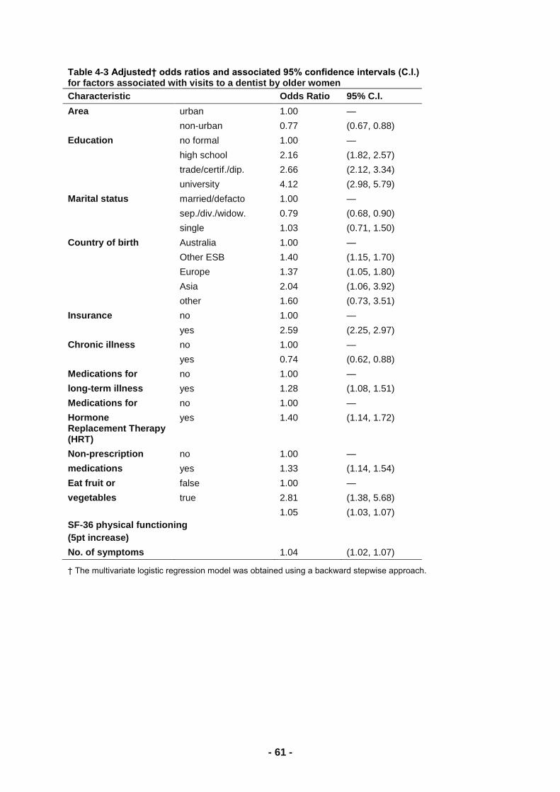
- 79 -
Factors associated with having a Pap test
Further analyses have been undertaken to assess the effect of area of residence on the probability
that women have had a Pap test within the past 2 years, after accounting for other socio-demographic
factors. For women in the 1973-78 cohort, the probability of having a Pap test in the past 2 years was
higher at Surveys 2, 3, 4 and 5 than at Survey 1, with the greatest difference being between Survey 1
and Survey 2. In contrast, the probability of having a Pap test decreased with each survey for women
in the 1946-51 cohort.
Area of residence was a significant factor for women in the 1973-78 cohort, but not for women in the
1946-51 cohort. Women in the 1973-78 cohort who lived in inner and outer regional areas were
around 10% more likely to have had a Pap test within the two year time frame than women living in
major cities.
Other factors affecting the probability of having a Pap test in the last two years for this cohort were
marital status, education, employment, health insurance and parity. Compared to married women,
widowed/separated/divorced women were around 21% less likely to have a Pap test, and single
women were around 56% less likely. Compared to women with no formal educational qualifications
or with a school certificate only, women were less likely to have a Pap test in the last two years if they
had achieved the higher school certificate, and more likely to have a Pap test if they had university or
higher education. Women working less than full time were less likely to have a Pap test than women
working full time. Women with private hospital insurance were more likely to have a Pap test than
those who did not have this cover, and women were more likely to have a Pap test if they had 1-3
children (compared to no children), but not if they had more than 3 children.
Fewer factors were associated with Pap tests among women in the 1946-51 cohort. Compared to
married women, women were less likely to have a Pap test if they were separated, divorced or
widowed, and much less likely to have a Pap test if they had remained single. Hospital insurance was
associated with increased probability of having a Pap test, and women with children (1 or more births)
were also more likely to have a Pap test than nulliparous women (no births).
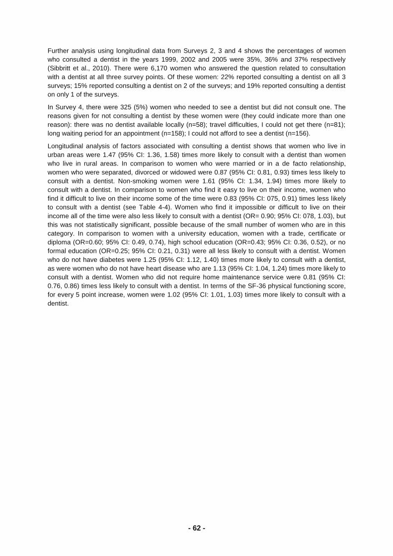
- 80 -
Table 4-9 Factors associated with having a Pap test in the past 2 years. 1973-78 and 1946-51 cohorts.
1973-78 cohort
Pap test
1946-51 cohort
Pap test
Variable OR (95% CI) OR (95% CI)
Survey 1 1
Survey 1 (ref) 1 1
Survey 2 1.70 (1.58, 1.83)* 1.01 (0.95,1.08)
Survey 3 1.78 (1.64, 1.93)* 0.99 (0.93,1.06)
Survey 4 1.49 (1.36, 1.62)* 0.87 (0.81,0.93) *
Survey 5 1.44 (1.31, 1.58)* 0.87 (0.81,0.93) *
Area of residence (ARIA)**
Major city 1 (reference)
Inner regional 1.24 (1.14, 1.33)*
Outer regional 1.34 (1.21, 1.49)*
Remote/v. Remote 1.21 (0.98, 1.50)
Marital status
Married/de facto 1 (reference) 1
Sep/div/widow 0.79 (0.70, 0.90)* 0.82 (0.75,0.89) *
Single 0.45 (0.42, 0.47)* 0.50 (0.42,0.60) *
Education
No formal qualification/sc 1 (reference)
HSC 0.81 (0.75, 0.88)*
Trade/diploma 1.02 (0.94, 1.11)
Higher educ. 1.10 (1.01, 1.20)*
Work
Full time 1 (reference)
Part-time 0.83 (0.79, 0.88)*
Other 0.73 (0.69, 0.77)*
Health insurance
No private insurance 1 (reference) 1
Private hospital insurance 1.14 (1.09, 1.20)* 1.38 (1.29,1.47) *
Parity
0 births 1 (reference) 1
1-3 births 1.545 (1.45, 1.66)* 1.52 (1.33,1.73) *
>3 births 1.22 (1.00, 1.48) 1.21 (1.04,1.42) *
*statistically significant p<0.05
**interaction between ARIA and survey was significant (p < 0.001) and adjusted for in the younger cohort, but not
displayed in table. It was not included in the 1946-51 cohort model as neither ARIA alone or as an interaction was significant.
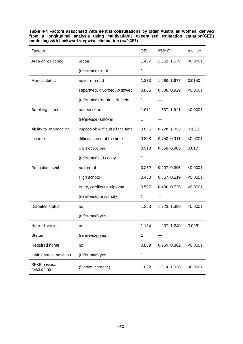
- 81 -
Discussion of trends in Pap testing
The collection of data on hysterectomies allows the ALSWH to provide valuable information on Pap
testing in the population at risk in a way that is not possible from most other data sources. The data
indicate that around 25-30% of women in the 1973-78 cohort and 20% in the 1946-51 cohort are not
having Pap tests within the recommended two-year screening interval (according to the women‘s self-
report). Allowing for some inaccuracy in self-report this percentage may be an underestimate or an
overestimate. As more opportunities for data linkage to screening registers become available, it will
be possible to extend these analyses and overcome some of these types of limitations.
4.6.2. Mammograms
Trends in self-reported time since last mammogram for the 1946-51 cohort are shown in Figure 4-31.
The proportion of women who had a mammogram within the last two years increased with each
survey and as the women aged. Note that at Survey 1, most women were younger than 50 years and
outside the age range of 50-69 years that is targeted for commencing routine screening
(http://www.cancerscreening.gov.au/internet/screening/publishing.nsf/Content/faqs#policy). By Survey
5, when women were aged 56-61 years, most had had a mammogram, but some women were
overdue for screening. By 2007 and depending on area, 25-30% of women in the 1946-51 cohort
could be considered ―overdue‖ for their next mammogram.
- 82 -
*Age 45-50 at Survey 1, 50-55 at Survey 3, 53-58 at Survey 4, and 56-61 at Survey 5
Figure 4-31 Self report of time since last Mammogram by women in 1946-51 cohort.
0% 10% 20% 30% 40% 50% 60% 70% 80% 90% 100%
Remote/Very Remote
Outer Regional
Inner Regional
S5Major Cities
Remote/Very Remote
Outer Regional
Inner Regional
S4Major Cities
Remote/Very Remote
Outer Regional
Inner Regional
S3Major Cities
Remote/Very Remote
Outer Regional
Inner Regional
S1Major Cities
< 2 years ago 2-5 years ago >5 yrs/don'tknow/never
- 83 -
Ease of obtaining a mammogram.
Most women in the 1946-51 cohort rated the ease of obtaining a mammogram as good, very good or
excellent. However, women in remote areas were less likely to give a favourable rating to this item
than women in major cities.
.
Figure 4-32 Ease of obtaining a Mammogram. 1946-51 cohort Survey 5
Factors associated with mammograms
Further analyses were undertaken to assess the effect of area of residence on the probability that
women have had a mammogram within the past 2 years, after accounting for other socio-
demographic factors (see Table 4-10). Women in this cohort were more likely to have a mammogram
over time, and as they aged, with women being around 4 times as likely to report a mammogram at
Survey 5 as at Survey 1. Women in remote areas were more likely to have a mammogram in the last
2 years than women in major cities, an interesting finding in light of the finding that they were the most
likely to report fair or poor access to this type of service.
Other factors associated with having a mammogram in the past 2 years included education (women
with tertiary or higher education were less likely to have had a mammogram) and marital status
(widowed, divorced, separated and single women were less likely to have had a mammogram).
Women with private hospital insurance were more likely to have had a mammogram, and women
were less likely to have had a mammogram if they had 3 or more children.
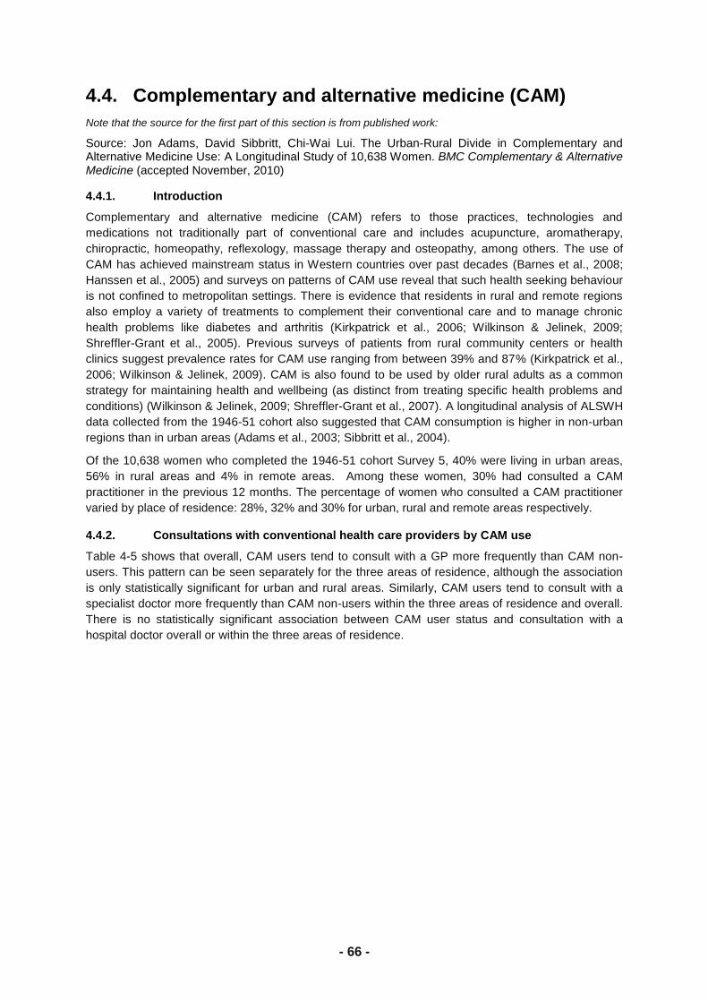
- 84 -
Table 4-10 Factors associated with having a mammogram in the past 2 years. 1946-51 cohort.
1946-51 cohort Mammogram
Variable OR (95% CI)
Survey
Survey 1 1 (reference)
Survey 2 1.44 (1.35, 1.54)*
Survey 3 2.69 (2.48, 2.93)*
Survey 4 3.38 (3.10, 3.69)*
Survey 5 3.77 (3.44, 4.13)*
Area of residence (ARIA+)**
Major city 1 (reference)
Inner regional 0.92 (0.85, 0.99)*
Outer regional 1.04 (0.94, 1.14)
Remote/v. Remote 1.43 (1.19, 1.71)*
Marital status
Married/de facto (ref) 1 (reference)
Sep/div/widow 0.80 (0.75, 0.85)*
Single 0.73 (0.63, 0.85)*
Education
None/sc 1 (reference)
HSC 0.95 (0.88, 1.02)
Trade/diploma 0.95 (0.88, 1.02)
Higher educ. 0.81 (0.74, 0.87)*
Health insurance
No private insurance 1 (reference)
Private hospital insurance 1.36 (1.30, 1.43)*
Parity
0 births 1 (reference)
1-3 births 1.01 (0.91, 1.12)
>3 births 0.83 (0.74, 0.94)*
*statistically significant p<0.05
**Interaction between Aria and survey was significant (p = 4.6%) and included in the model, but not reported here.
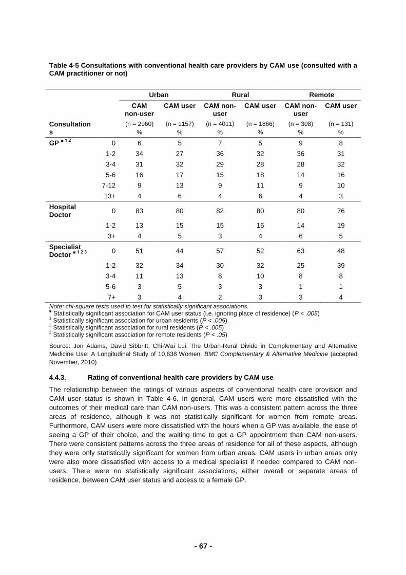
- 85 -
4.6.3. Discussion
The collection of data on hysterectomies allows the ALSWH to provide valuable information on Pap
testing in the population at risk in a way that is not possible from other data sources. The data
indicate that, depending on area, around 25-30% of women in the 1973-78 cohort and 20% in the
1946-51 cohort did not have Pap tests within the recommended two-year screening interval
(according to the women‘s self-report). Allowing for some inaccuracy in self-report, mainly due to
women under-estimating the time since their last Pap test, this percentage may be an underestimate.
There is a trend for women in the 1973-78 cohort to be less likely to be overdue for a Pap test as they
move through their 20s (the 1973-78 cohort) and for women in the 1946-51 cohort to become more
likely to be overdue for a Pap test after their 50s. Other socio-demographic factors also affect the
probability women will be screened, with lower rates of screening among unmarried women, those
with high school education only, less than full-time employment, no private health insurance and
those who have not had children. Women in the 1973-78 cohort living in regional areas were less
likely to be screened than women in urban or remote areas. There were no area differences for the
1946-51 cohort.
The probability that women in the 1946-51 cohort had a mammogram within two years increased with
each survey and as more women reached 50 years, the age promoted as when screening should
start. There were few differences in screening by area, except women in remote areas were the most
likely to be screened. Other sociodemographic factors associated with higher probability of having a
mammogram included being married and having private insurance. Women with three or more
children and those with higher education were less likely to be screened.
Younger women and women in remote areas reported more difficulty accessing screening tests.
However self-reported screening rates which suggest that women in remote areas are more likely to
be screened in-spite of these access difficulties.
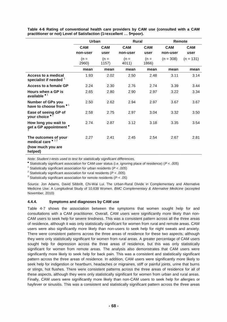
- 86 -
5. Out of pocket costs for medical
services by geographic location
5.1. Introduction
Access to bulk billed medical services has been an important mechanism for improving equity in
access to health care for people in Australia. In 2003, Young and Dobson (2003) published data that
demonstrated a steady decline in bulk-billing for general practice consultations for ALSWH
participants living in rural areas between 1995 and 2001, and that use of bulk billing was substantially
lower in rural areas than in urban areas. After adjusting for age, health and socioeconomic factors,
women living in urban areas were more than twice as likely to have all their consultations bulk-billed
as women living in rural areas (see Figure 5-1).
Since that time, there have been substantial changes to Medicare to encourage bulk billing,
particularly in remote areas.
During 2004 Medicare introduced new item numbers which allowed medical practitioners (mainly
GPs) to claim an additional Medicare rebate for bulk billed services provided to Commonwealth
concession card holders or children aged under 16 years. Under these arrangements, practitioners
could claim an extra $5.00 (now $5.75, effective January 2011) for concession card holders and
children, and $7.50 (now $8.75, effective January 2011) for services provided to eligible patients in
areas 3-7 in the Rural Remote Metropolitan Areas (RRMA) classification, in any one of 29 eligible
metropolitan areas where there is a shortage of GPs, or where bulk billing rates were below the
national average, or anywhere in Tasmania (Medicare Australia 2005a; Medicare Australia 2005b).
In this section of the report, we explore whether these new Medicare incentives have had an impact
on bulk billing over recent years, and particularly whether they have reduced the inequity in access to
bulk billing in regional and remote areas. To do this, we analysed Medicare data on out-of-pocket
costs for GP services for the years 2002-2008 for women in the three ALSWH cohorts who consented
to access to Medicare data and who responded to Survey 5 (conducted in 2007 for the 1946-51
cohort then aged 56-61 years, in 2008 for the 1921-26 cohort, then aged 82-87, and in 2009 for the
1973-78 cohort, then aged 31-36).
All claims for services (including GP consultations) that were processed by Medicare Australia for
consenting women for the period 2002-2008 were extracted by Medicare and forwarded to us for
analysis. The unit records included the woman's identification number for the study, postcode, date of
service, type of billing, charge and Medicare rebate for each service provided. GP consultations were
defined as services with item numbers 1-98, 601, 602, 697 or 698 in the Medicare Benefits Schedule.
For these analyses, Medicare data were available for 4329 women in the 1973-78 cohort, 7095
women in the 1946-51 cohort and 4120 women in the 1921-26 cohort who had consented to the
release of Medicare data and responded to Survey 5.
For bulk-billed GP consultations, the out-of-pocket cost was defined as zero. For all other
consultations, the cost was calculated as the difference between the amount charged by the provider
and the Medicare rebate for the service (which includes the "safety net" payment, where applicable).
The mean out-of-pocket cost for each woman for each calendar year was calculated, provided that
she had had at least one consultation in that year (women with no claims were not included in these
data as they had no visits to the GP subsidised under Medicare and therefore no opportunity to be
bulk billed). The mean out-of-pocket cost was categorised as $0, >$0 to ≤ $5, > $5 to ≤ $10, or > $10
per consultation. To allow for the effects of inflation, costs for all years were adjusted to 2008 dollar
values using the consumer price index published by the Australian Bureau of Statistics (ABS) for the
June quarter of each year (ABS, 2008).
- 87 -
For each year in the period 2002-2008, the mean out-of-pocket cost per consultation for each woman
was summarised by cohort and ARIA+ category
Figure 5-1 Out of pocket costs for GP services since 1995-2001.
Source: Young AF, Dobson AJ. The decline in bulk billing and increase in out-of-pocket costs in general practice consultations in rural Australia, 1995-2001. Medical Journal of Australia 2003; 178: 122-126
Out-of-pocket costs for GP services since 2002 are shown in Figure 5-2, Figure 5-3 and Figure 5-4.
In 2002, 61% of women in the 1921-26 cohort in city areas had a mean cost of $0 per consultation,
and in 2003 this proportion fell to 55% in city areas and was lower for women in regional and remote
areas. From 2005 onwards and across all areas, there was a marked increase in the proportion of
women in this cohort with no out of pocket costs for GP consultations. The greatest increases were
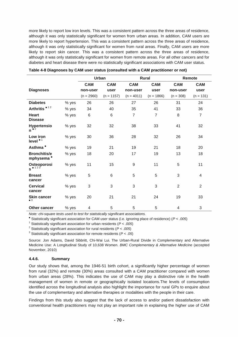
- 88 -
observed in remote and very remote areas. The inner regional areas were most disadvantaged in
terms of bulk billing, even after the introduction of the bulk billing incentives.
Compared to the 1921-26 cohort, women in the 1973-78 and 1946-51 cohorts, were less likely to
have no out-of-pocket costs across all years and all areas and showed less dramatic increases in bulk
billing following the introduction of incentives (supplementary figures available). As for older women,
1973-78 and 1946-51 cohort women in inner regional areas were less likely to be bulk billed.
- 89 -
Figure 5-2 Mean out-of pocket cost per general practice consultation per woman per year, 2002-2008, for women born in 1921-26 by area of residence, adjusted to 2008 dollar values.
** Note: General practice consultations were defined as services with item numbers 1-98, 601, 602, 697 or 698 in the Medicare Benefits Schedule
Major City Inner Regional
Outer Regional Remote/Very Remote
0%
20%
40%
60%
80%
100%
2002 2003 2004 2005 2006 2007 2008
>$10 >$5 to <=$10 >$0 to <=$5 $0
0%
20%
40%
60%
80%
100%
2002 2003 2004 2005 2006 2007 2008
>$10 >$5 to <=$10 >$0 to <=$5 $0
0%
20%
40%
60%
80%
100%
2002 2003 2004 2005 2006 2007 2008
>$10 >$5 to <=$10 >$0 to <=$5 $0
0%
20%
40%
60%
80%
100%
2002 2003 2004 2005 2006 2007 2008
>$10 >$5 to <=$10 >$0 to <=$5 $0
- 90 -
Figure 5-3 Mean out-of pocket cost per general practice consultation per woman per year, 2002-2008, for women born in 1946-51 by area of residence, adjusted to 2008 dollar values.
Major City Inner Regional
Outer Regional Remote/Very Remote
0%
20%
40%
60%
80%
100%
2002 2003 2004 2005 2006 2007 2008
>$10 >$5 to <=$10 >$0 to <=$5 $0
0%
20%
40%
60%
80%
100%
2002 2003 2004 2005 2006 2007 2008
>$10 >$5 to <=$10 >$0 to <=$5 $0
0%
20%
40%
60%
80%
100%
2002 2003 2004 2005 2006 2007 2008
>$10 >$5 to <=$10 >$0 to <=$5 $0
0%
20%
40%
60%
80%
100%
2002 2003 2004 2005 2006 2007 2008
>$10 >$5 to <=$10 >$0 to <=$5 $0
- 91 -
Figure 5-4 Mean out-of pocket cost per general practice consultation per woman per year, 2002-2008, for women born in 1973-78 by area of residence, adjusted to 2008 dollar values.
Major City Inner Regional
Outer Regional Remote/Very Remote
0%
20%
40%
60%
80%
100%
2002 2003 2004 2005 2006 2007 2008
>$10 >$5 to <=$10 >$0 to <=$5 $0
0%
20%
40%
60%
80%
100%
2002 2003 2004 2005 2006 2007 2008
>$10 >$5 to <=$10 >$0 to <=$5 $0
0%
20%
40%
60%
80%
100%
2002 2003 2004 2005 2006 2007 2008
>$10 >$5 to <=$10 >$0 to <=$5 $0
0%
20%
40%
60%
80%
100%
2002 2003 2004 2005 2006 2007 2008
>$10 >$5 to <=$10 >$0 to <=$5 $0
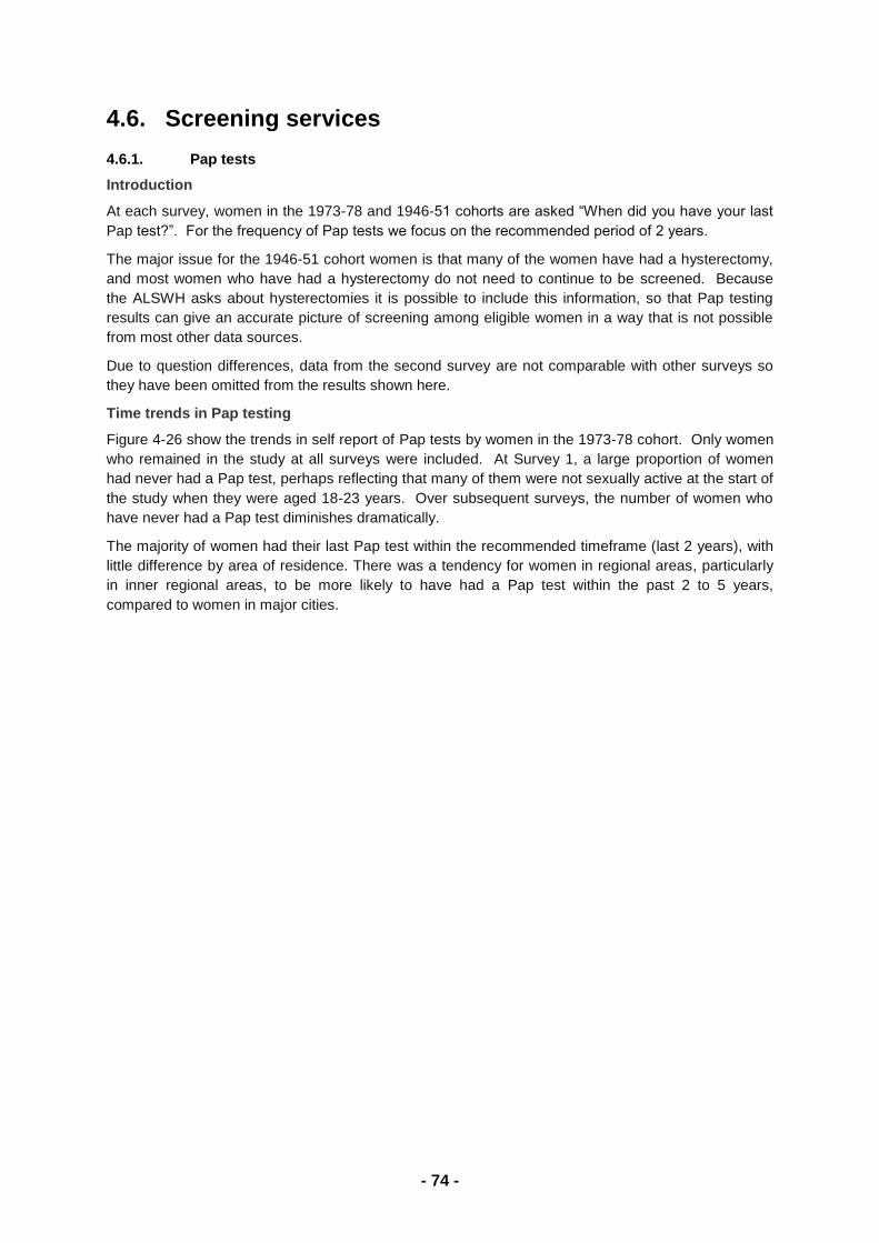
- 92 -
Comparisons of the proportions of women with zero out-of-pocket costs in 2008 show that women in
the 1921-26 cohort and those in remote areas are most likely to have zero out of pocket costs. For
instance, among women in the 1921-26 cohort, 87% of women in remote/very remote areas had no
out-of-pocket costs for GP services in 2008, compared with 75% of women in city areas
Table 5-1 Proportions of women with zero out of pocket costs for general practitioner services in 2008
1973-78 cohort
N= 3129
1946-51 cohort
N=6227
1921-26 cohort
N=4077
City 30% 34% 75%
Inner regional 23% 29% 68%
Outer regional 26% 37% 75%
Remote/very remote 38% 44% 87%
5.2. Discussion
Results for recent years demonstrate an overall improvement in access to bulk-billing following
introduction of incentives in 2004, although some geographical inequity remains particularly for
women in inner regional areas. The results contrast with earlier findings reported by Young and
Dobson (2003) showing declining rates of bulk-billing and increasing out-of-pocket costs, particularly
in rural areas. The authors expressed concern about the increasing costs for women in the 1921-26
cohort and called for policy changes to enable women in rural and remote areas to have better access
to affordable healthcare services. The dramatic increases in bulk billing and reduction in out-of-
pocket costs, particularly for older women in remote areas show a reversal of this earlier trend
following the policy change.
A strength of this study is that the results are based on a national random sample of women rather
than a sample of people attending particular general practices, and so the findings can be more
readily generalised to the population. A limitation is that women who consented to record linkage had
a higher level of education than women who did not consent to linkage (Young et al., 2001). This
socioeconomic bias between consenters and non-consenters may result in an under-estimate of the
proportions of women who have all their consultations bulk-billed. However, trends over time showing
the increasing use of bulk-billing and decreasing out-of-pocket costs would be unaffected by any
socioeconomic bias in the sample of consenters. There were also small differences between
consenters and non-consenters to release of Medicare data according to area of residence, but these
are not likely to affect the geographical differences demonstrated in our study.
Another limitation is that women were classified according to their residence at Survey 5, which may
not reflect their area of residence classification across the entire observation period. However
women‘s residential classifications tend to be quite stable over time, particularly for the older cohort.
While the bulk billing incentives are aimed at areas defined under the RRMA classification, we have
analysed our data according to ARIA+ which is now the standard classification of accessibility and
remoteness and which is stable over time. Our analysis shows a relative disadvantage for women in
inner regional areas (under the ARIA+ classification) which are not necessarily covered under the
RRMA-based incentives scheme. The results suggest that the incentives could be further evaluated
to assess the potential for reducing inequity for inner regional areas, as well as more remote areas.
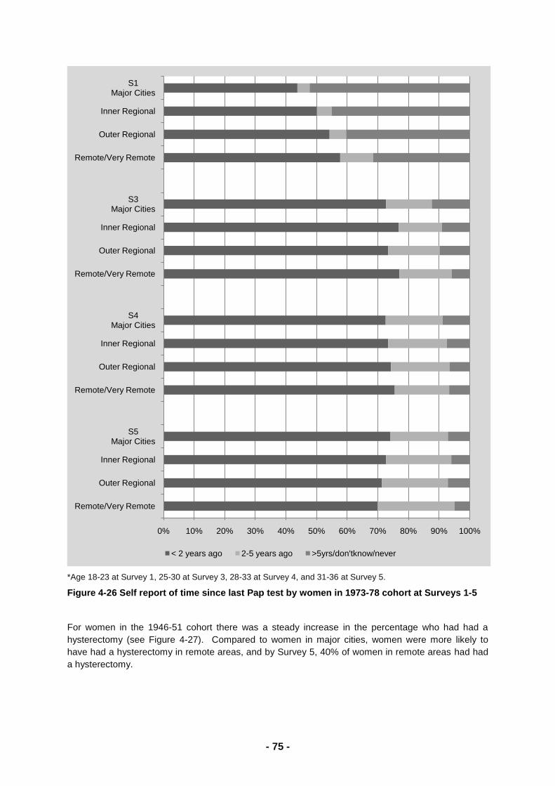
- 93 -
5.3. Conclusion
Access to bulk billing has improved in the years following the introduction of Medicare incentives for
bulk billing, particularly in remote areas and for older women. Some inequity remains for women in
inner regional areas and further evaluation of the scheme is required to reduce this inequity while
maintaining the improved access for people in remote areas.
5.4. References:
Young A, & Dobson A. (2003). The decline in bulk billing and increase in out-of-pocket costs for
general practice consultations in rural areas of Australia, 1995-2001. Medical Journal of
Australia, 178: 122-126.
Medicare Australia (2005a). Incentive payments to GPs who bulk bill concessional patients and
children aged under 16
years.http://www.medicareaustralia.gov.au/provider/incentives/files/incentive_payments_to_GP
s_who_bulk_bill_concessional_patients_under_16.pdf (last accessed 25 September 2010)
Medicare Australia (2005b). Annual Report 2004-2005.
http://www.medicareaustralia.gov.au/about/governance/reports/04-05/index.jsp (last accessed
25 September 2010)
Young AF, Dobson AJ, & Byles JE. (2001). Health services research using linked records: Who
consents and what is the gain? Australian and New Zealand Journal of Public Health, 25: 417-
420.
Australian Bureau of Statistics. (2008). 6401.0 - Consumer Price Index, Australia, Dec 2008
http://www.ausstats.abs.gov.au/Ausstats/subscriber.nsf/0/E770454272374338CA25754B0014
CD2C/$File/64010_dec%202008.pdf (last accessed 25 September 2010).
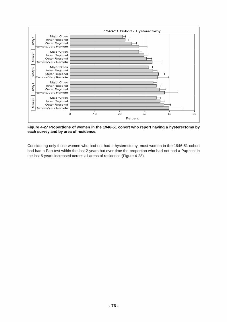
- 94 -
6. Differences in birth interventions by
geographic location
6.1. Introduction
The aims of this study were to investigate differences in birth interventions by geographic location and
to determine whether these differences could be explained by other characteristics of the mothers
rather than where they live. For example, women living in regional and remote areas tend to have
their babies earlier, are less educated and less likely to have private health insurance than women
living in major cities.
This analysis includes women in the 1973-78 cohort who had given birth to their first child between
1994 and 2010 and had provided details for those births. Half the births were to women living in major
cities and more than half of the women had private health insurance.
6.2. Birth interventions by area of residence
The distribution of birth interventions are shown by area of residence in the following Figures.
Figure 6-1 shows that the percentage of first-time mothers who had experienced prolonged labour
was the same across area of residence.
Figure 6-1 Prolonged labour by area of residence.
Figure 6-2 shows the percentage of first-time mothers who had experienced emotional distress was
also the same across area of residence.
0% 20% 40% 60% 80% 100%
Remote/Very Remote
Outer Regional
Inner Regional
Major Cities
Prolonged labour Labour less than 36 hours
- 95 -
Figure 6-2 Emotional distress by area of residence
Although length of labour and emotional distress were the same across areas, women living in major
cities were more likely to have pain relief than women living in regional and remote areas (Figure 6-3).
In addition women living in major cities were more likely to have an epidural injection than other
women.
Figure 6-3 Type of pain relief by area of residence
More than half the women living in major cities had an instrumental delivery, with almost 30% having an elective or emergency caesarean (Figure 6-4). In comparison, 21% to 25% of women living outside major cities had a caesarean.
Figure 6-4 Type of delivery by area of residence
0% 20% 40% 60% 80% 100%
Remote/Very Remote
Outer Regional
Inner Regional
Major Cities
Emotional distress No emotional distress
0% 20% 40% 60% 80% 100%
Remote/Very Remote
Outer Regional
Inner Regional
Major Cities
No pain relief Epidural Gas/injection Epidural and gas
0% 20% 40% 60% 80% 100%
Remote/Very Remote
Outer Regional
Inner Regional
Major Cities
Non-instrumental delivery Forceps or Ventous suction
Elective caesarean Emergency caesarean
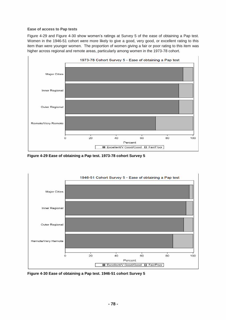
- 96 -
Figure 6-5 shows the percentage of first-time mothers who had an episiotomy or a vaginal tear
requiring stitches by area of residence. There were no significant differences between these
interventions across area.
Figure 6-5 Episiotomy or vaginal tear requiring stitches by area of residence
After adjusting for differences in age, education level and private health insurance, women living
outside major cities had lower odds of having an epidural injection. This was statistically significant for
women living in remote or very remote areas and women living in inner regional areas. Women living
in remote or very remote areas had lower odds of having other pain relief than women living in major
cities. Women with private health insurance had 2.5 times the odds of having an epidural than women
without private health insurance.
Age was the major explanatory variable for the differences in type of delivery seen across area.
Compared with women in their early twenties, women in their late twenties had two to three times the
odds of having an instrumental delivery and women in their thirties had two times the odds of having a
forceps or suction delivery and three to four times the odds of having a caesarean.
The same pattern of birth interventions was seen across area of residence for the birth of the second
child (data not shown), but interventions were less common for all interventions other than elective
caesareans. Prolonged labour was experienced by less than 2% of women and emotional distress by
14% to 16%. Almost 30% of women living in major cities had an epidural compared with 20% of
women living outside major cities. Non-instrumental deliveries occurred in 68% to 69% of women
living in major cities and inner regional areas, and 75% to 77% of women living in outer regional and
remote or very remote areas.
6.3. Risk factors for having an epidural or spinal block
Clearly women living in major cities were more likely to have an epidural or spinal block. More
detailed analysis of risk factors for having an epidural or spinal block for the birth of the first baby was
conducted. Risk factors included sociodemographic factors (age, area of residence, marital status,
educational qualifications, employment, hours worked, feeling stressed about money and private
health insurance), health behaviours (prior smoking, alcohol consumption and exercise), and other
health-related factors (body mass index, height, stress about own health and diagnosis with diabetes,
hypertension, depression and anxiety). In unadjusted models, sociodemographic factors that were
significantly related to having an epidural were age, area of residence, marital status, educational
qualifications, employment, hours worked and private health insurance. Health-related factors
included prior alcohol consumption, body mass index, height, diagnosed anxiety and depression.
In adjusted models, age, area of residence, private health insurance, body mass index and height
remained significant. Figure 6-6 shows the percentage of first-time mothers who had an epidural or
0% 20% 40% 60% 80% 100%
Remote/Very Remote
Outer Regional
Inner Regional
Major Cities
No episiotomy or tear Episiotomy Vaginal tear Episiotomy or tear
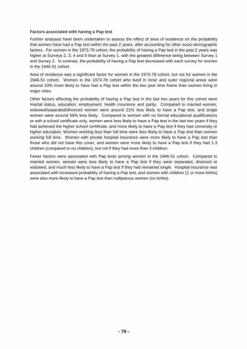
- 97 -
spinal block by age of the mothers. Almost 60% of first-time mothers aged over 30 had an epidural or
spinal block, compared with 37% of first-time mothers aged 15 to 24 years.
Figure 6-6 Epidural or spinal block by age of first-time mother
The percentage of first-time mothers who had an epidural or spinal block is shown by private health
insurance in Figure 6-7. Almost 60% of women with private health insurance had an epidural or spinal
block compared with 44% of women without private health insurance.
Figure 6-7 Epidural or spinal block by private health insurance
In Figure 6-8, the percentage of women who had an epidural or spinal block is shown by body mass
index group. The risk of an epidural increased with increasing body mass index, with two thirds of
obese women having an epidural compared with half the women with acceptable weight.
Figure 6-8 Epidural or spinal block by body mass index group
0% 20% 40% 60% 80% 100%
30-36 years
25-29 years
15-24 years
Epidural No Epidural
0% 20% 40% 60% 80% 100%
No private health insurance
Private health insurance
Epidural No Epidural
0% 20% 40% 60% 80% 100%
Underweight
Acceptable weight
Overweight
Obese
Epidural No Epidural
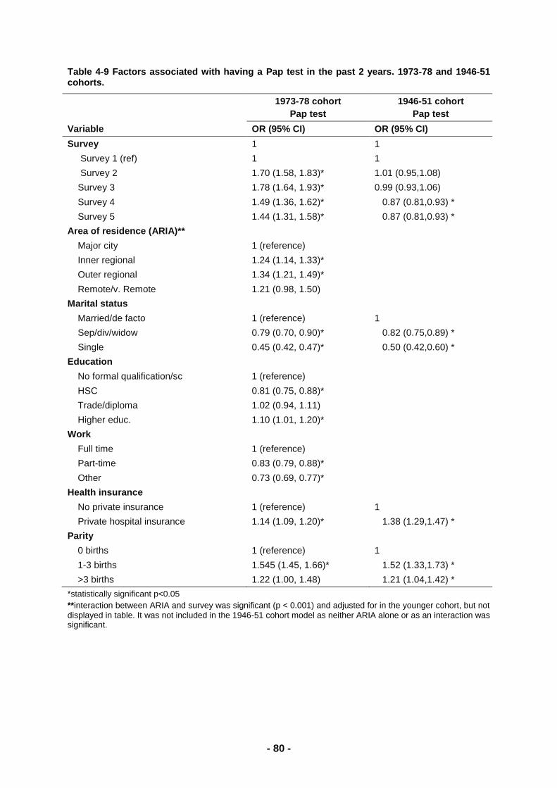
- 98 -
Figure 6-9 shows the percentage of women who had an epidural or spinal block by height. Shorter
women were more likely to have an epidural than taller women.
Figure 6-9 Epidural or spinal block by height
In the final adjusted model, the odds of first-time mothers having an epidural or spinal block were
higher among women aged 25 or more, those with private health insurance, short women and women
who were overweight or obese. The odds of women having an epidural or spinal block were lower
outside major cities, and significantly lower for women living in inner and outer regional areas.
6.4. Risk factors for having a caesarean
More first-time mothers living in major cities had emergency or elective caesarean section. Logistic
regression models were used to compare risk factors for an emergency caesarean to a vaginal
delivery and elective caesarean to a vaginal delivery. The models included the same risk factors used
in the epidural models: sociodemographic factors (age, area of residence, marital status, educational
qualifications, employment, hours worked, feeling stressed about money and private health
insurance), health behaviours (smoking, alcohol consumption and exercise), and other health-related
factors (body mass index, height, stress about own health and diagnosis with diabetes, hypertension,
depression and anxiety). Two models were fitted for each type of caesarean section; one included
having an epidural or spinal block, the other did not.
In unadjusted models for an emergency caesarean, maternal age, hours worked, private health
insurance, body mass index, height, diagnosis of diabetes and having an epidural or spinal block
were all significant. In both adjusted models, the odds of an emergency caesarean were one and a
half to two times higher among first-time mothers who were older, had higher body mass index and
shorter height. However the odds of an emergency caesarean were more than 16 times higher among
women who had had an epidural or spinal block than those who had not.
Maternal age, area of residence, private health insurance, prior alcohol consumption, body mass
index, short stature, diagnosis of diabetes, diagnosis of hypertension, diagnosed depression,
diagnosed anxiety and having an epidural or spinal block were all significant in unadjusted models for
elective caesarean. In the adjusted models, the odds of an elective caesarean were twice as high in
women aged over thirty and in obese women and one and a half times higher in women with
diagnosed anxiety. In the adjusted model excluding having an epidural, the odds of an elective
caesarean were 1.6 times as high among women with private health insurance, however this was no
longer significant once having an epidural was included in the model. The odds of an elective
caesarean were more than 12 times higher among women who had had an epidural or spinal block
than those who had not.
0% 20% 40% 60% 80% 100%
Taller height
Short height
Epidural No Epidural
- 99 -
6.5. Key issues:
Prolonged labour and emotional distress do not differ across area or residence, but use of
pain relief is higher in major cities.
Pain relief is more commonly administered in the form of an epidural or spinal block in major
cities, whereas gas or an injection is more common in inner and outer regional areas.
Elective and emergency caesareans are more common in major cities. However, once age
and private health insurance are taken into account, differences across area are no longer
significant.
Odds of elective caesareans among first-time mothers in their thirties are four times the odds
among first-time mothers in their early twenties. If the age of first-time mothers continues to
rise, more specialists and hospital beds will be required to cope with the increased rate of
elective caesarean operations for the first birth. In addition, having a prior caesarean
increases the risk of subsequent caesareans.
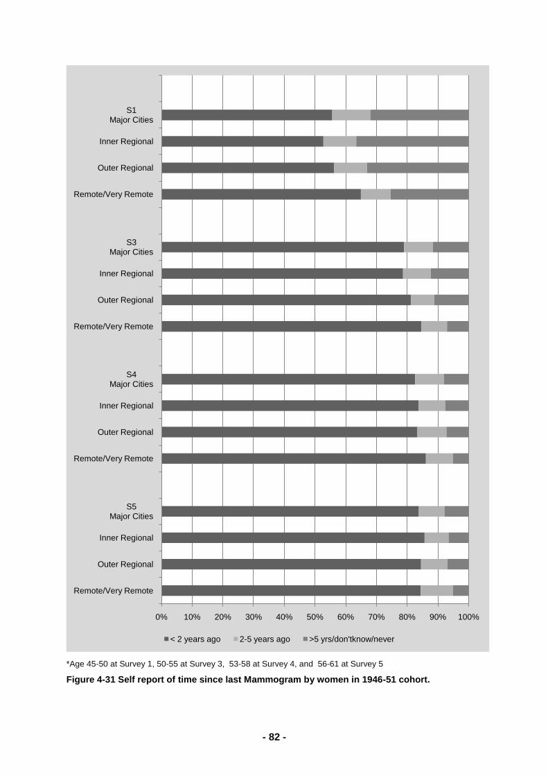
- 100 -
7. Climate events and women’s health
7.1. Exceptional circumstances and mental health
Much has been written about the potential effects of climate change on health, however empirical
evidence on the impact of climate change on health is scarce. One reason for the scarcity of evidence
is the difficulty in measuring climate change. It is generally accepted that climate change will result in
a worse climate and more prolonged adverse climate conditions. Hence this project used a
declaration of Exceptional Circumstances (EC) as a proxy indicator of climate change. The Australian
Government may declare an EC area if there is a one in 20-25 year event such as drought, flood or
fire that results in a severe downturn in farm or farm-related income. People living in EC areas may
apply for financial support and interest rate subsidies.
The aim of this project was to compare the health and well-being of ALSWH participants living in EC
and non-EC areas. Based on where women were living at the time of the fourth survey (2004/5) of the
1946-51 cohort, women were classified as living in an EC or non-EC area. This analysis includes
6584 women who were living outside major cities.
Selected characteristics of women living in EC areas are shown in the Figures below. Women living in
EC areas were more likely to live in inner regional areas (Figure 7-1).
Figure 7-1 Distribution of women living in Exceptional Circumstances declared areas by ARIA+
Women living in EC areas had slightly more difficulty managing on available income (Figure 7-2).
0% 20% 40% 60% 80% 100%
Remote/Very Remote
Outer Regional
Inner Regional
Exceptional Circumstances No Exceptional Circumstances
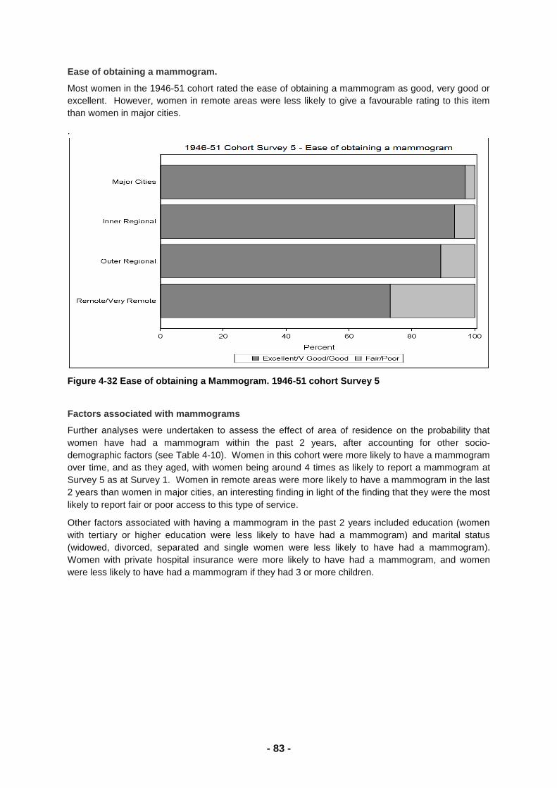
- 101 -
Figure 7-2 Ability to manage on available income by Exceptional Circumstances
Women living in EC areas had the same levels of social support and perceived control as women
living in non-EC areas. Women living in EC areas were less optimistic than their counterparts in non-
EC areas (Figure 7-3).
Figure 7-3 Level of optimism for women living in Exceptional Circumstances and non-Exceptional Circumstances area
Women living in EC areas were just as likely to have five or more general practitioner visits in the last
year, to report doctor diagnosed physical conditions and to report doctor diagnosed depression or
anxiety. Less than one percent of women in EC and non-EC areas had deliberately self-harmed
themselves in the past six months.
The self-rated quality of life subscales of the SF-36 (General Health and Mental Health) did not differ
for women living in EC and non-EC areas in 2004. Nor were there differences in these scores for the
same women in 1996 or for the change in scores between 1996 and 2004. There was a small
difference in perceived stress scores in 2004, with women in EC areas showing slightly more stress.
The difference in perceived stress disappeared when statistical models were adjusted for
demographic factors.
This project found no health deficit associated with living in an EC area. Some limitations of the study
may explain these negative findings. Firstly, EC is a coarse measure of adverse climate conditions
and may not differentiate very severe climactic events that would be associated with climate change.
Secondly, the analysis only included women aged 53 to 58 years and women in this age group may
0% 20% 40% 60% 80% 100%
Difficult
Not too bad
Easy
Exceptional Circumstances No Exceptional Circumstances
0% 20% 40% 60% 80% 100%
Low
Moderate
High
Exceptional Circumstances No Exceptional Circumstances
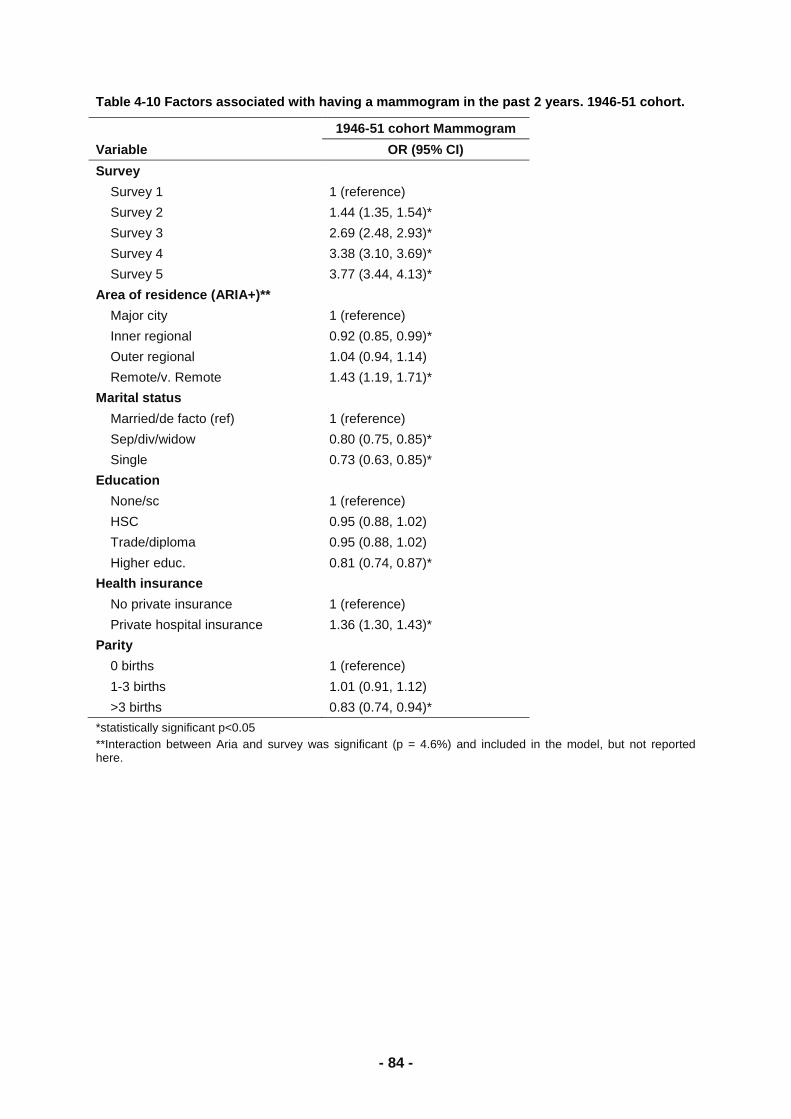
- 102 -
not only be more resilient than women in other age groups, but also may be more able to cope than
men.
Although there was no information about whether women were actually receiving EC assistance, it is
possible that the recognition that assistance would be available to people in need may be sufficient to
bolster women‘s health.
7.2. Precipitation and self rated health
This section builds on Section 7.1 by examining changes in the health and well-being of women in
relation to long term variations in rainfall. Based on where women lived, data from the first five
surveys of the 1946-51 cohort were linked to the Bureau of Meteorology (BOM) monthly climate data.
An indicator of dry conditions was calculated for each month based on rainfall in the six months up to
and including the current month. The indicator was 1 if rainfall was below a threshold level relative to
rainfall over the same six months between 1890 and 2008 (Smith et al., 1992). The indicator was 0 if
rainfall was at or above threshold and indicated that dry conditions were not present for the six
months culminating in that month. The indicator was used to define dryness, when between one and
four consecutive months had an indicator of 1, and drought when five or more consecutive months
had an indicator of 1.
The aim of this project was to determine whether drought or dryness resulted in poorer health and
well-being. This analysis includes 8609 women who were living outside major cities in 1996.
The presence of drought or dryness across Australia, excluding the Northern Territory and offshore
islands, is shown by Survey year in Figure 7-4. There have been considerable fluctuations in dryness
and drought over the 12 years, with the worst drought conditions occurring in 1998 and 2007 and
extensive dry conditions occurring in 2004. Over half the women were affected by dryness or drought
in 1998, 2004 and 2007, whereas in 1996, a quarter of the women were affected by dryness or
drought.
Figure 7-4 Distribution of dryness and drought across Australia by Survey year for the 1946-51 cohort.
0% 20% 40% 60% 80% 100%
2007
2004
2001
1998
1996
No drought or dryness Dryness Drought
- 103 -
Selected characteristics of women living in areas affected by dryness or drought in 2007 are shown in
the Figures below. Women living in drought areas had no more difficulty managing on available
income than women living in areas not affected by drought or dryness (Figure 7-5).
Figure 7-5 Ability to manage on available income by dryness and drought in 2007 for ALSWH participants in the 1946-51 cohort.
Women living in drought areas had the slightly higher levels of social support than women living in
areas not affected by dryness or drought (Figure 7-6).
Figure 7-6 Level of social support by dryness and drought in 2007 for ALSWH participants in the 1946-51 cohort.
Women living in dry and drought areas had the slightly higher levels of perceived control than women
living in areas not affected by dryness or drought (Figure 7-7).
Figure 7-7. Level of perceived control by dryness and drought in 2007 for ALSWH participants in the 1946-51 cohort.
0% 20% 40% 60% 80% 100%
Drought
Dryness
No drought or dryness
Not too bad Difficult
0% 20% 40% 60% 80% 100%
Drought
Dryness
No drought or dryness
High Moderate Low
0% 20% 40% 60% 80% 100%
Drought
Dryness
No drought or dryness
High Moderate Low
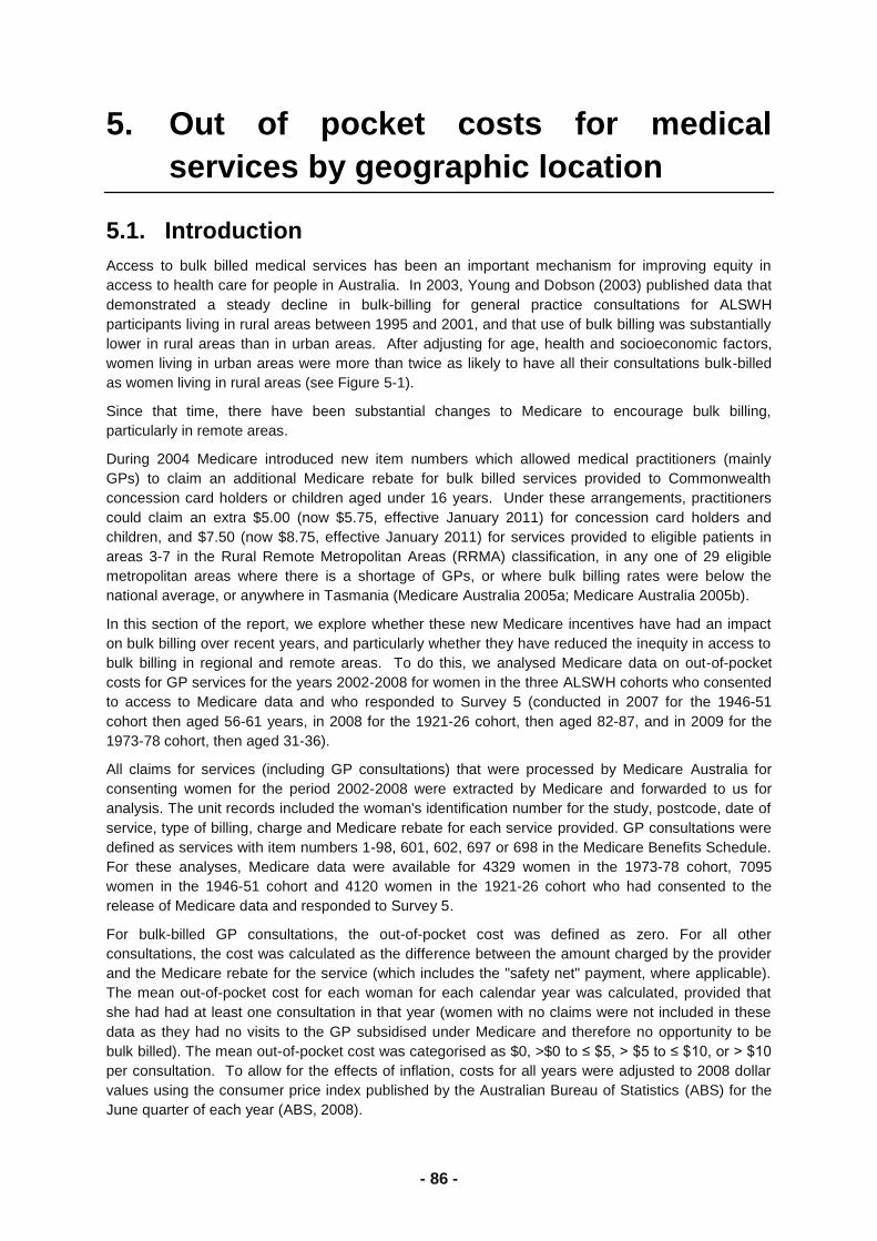
- 104 -
Levels of optimism were similar for women living in dry and drought areas and women living in areas
not affected by dryness or drought (Figure 7-8)
Figure 7-8 Level of optimism by dryness and drought in 2007 for ALSWH participants in the 1946-51 cohort.
Regardless of conditions, around 6% of women felt that life was not worth living and less than 1% of
women had deliberately harmed themselves.
The self-rated quality of life subscales of the SF-36 (General Health and Mental Health) did not differ
for women living in areas affected by dryness and drought between 1996 and 2007 (Figure 7-9 and
Figure 7-10). Nor were there differences in perceived stress scores over the same time.
Figure 7-9 Changes in General Health over time by dryness and drought for ALSWH participants in the 1946-51 cohort.
0% 20% 40% 60% 80% 100%
Drought
Dryness
No drought or dryness
High Moderate Low
68
70
72
74
1996 1998 2001 2004 2007
No drought or dryness Dryness Drought
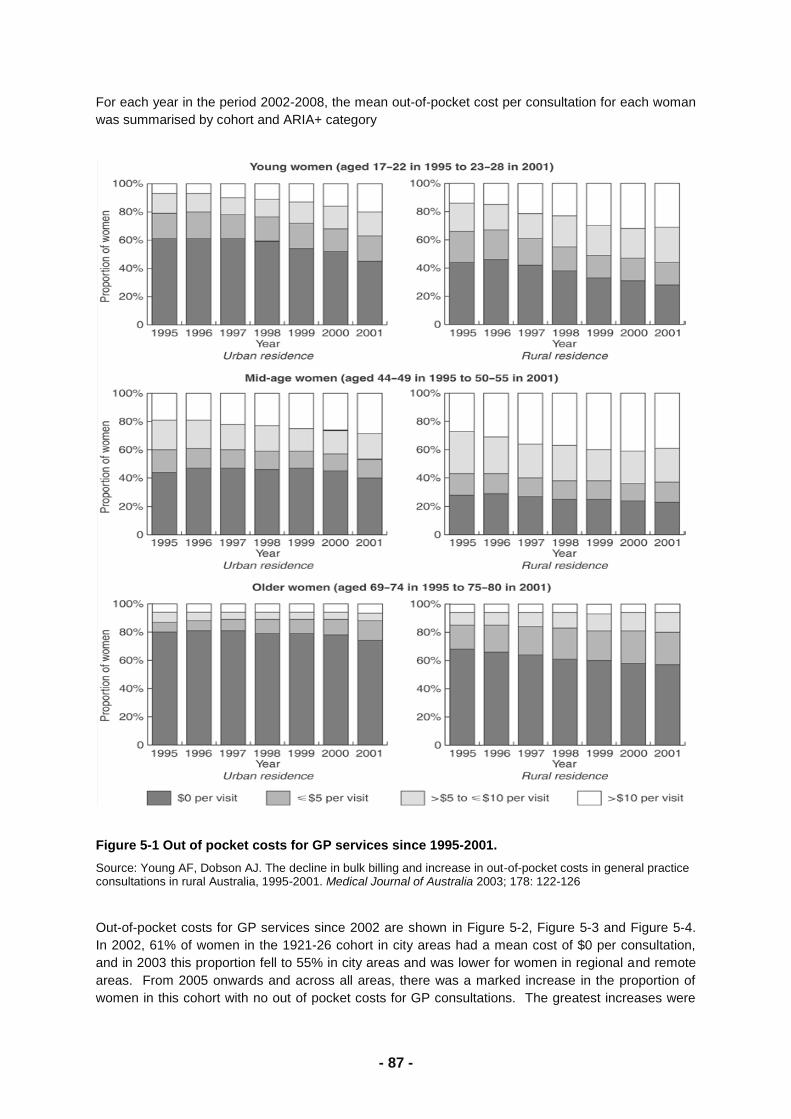
- 105 -
Figure 7-10 Changes in Mental Health over time by dryness and drought for ALSWH participants in the 1946-51 cohort.
Despite considerable fluctuations in dryness and drought between 1996 and 2007, this project found
no effect of dryness or drought on the health of women in the 1946-51 cohort. The measures of
General Health and Mental Health are recognised and sensitive measures of health and well-being. It
is possible that women in these age groups are sufficiently resilient that they can cope with dryness
and drought.
7.3. Soil salinity
Mental health of women in salinity affected areas in south west Western Australia.
Many areas of Australia are currently experiencing environmental degradation and adverse climatic
conditions which could be harmful to human health. One particular form of such environmental
degradation is soil salinisation (dryland salinity) which is a relatively a slow change caused by the
removal of deep rooted perennial native vegetation and its replacement with shallow rooted annual
crops. The change results in the rise of the water table which mobilises salt in the soil profile and
brings it to the surface. Several regions within Australia currently have substantial areas of land
affected by dryland salinity, the largest of which are in the south-west agricultural region of Western
Australia (WA).
We conducted a detailed analysis of the quantitative relationship between women‘s mental health and
salinity, as well as two other indicators of environmental degradation and change: land surface
temperature (LST) and normalised difference vegetation index (NDVI), a proxy for rainfall. We used
data from all three ALSWH cohorts for women living in the affected areas in south-west WA. Location
specific environmental measurements were linked to a mental health measure (MCS from the SF-36
health-related quality of life questionnaire) using the latitude and longitude calculated from the
women‘s addresses.
Bayesian linear regression models were developed to assess associations between environmental
exposures and mental health scores of women, with education level and ability to manage on income
included in models as socioeconomic measurements. To account for spatial autocorrelation in mental
health scores, geostatistical random effects were added to multivariable models using a Bayesian
framework.
For the 1973-1978 cohort, the only individual-level variable significantly associated with mental health
score was ability to manage on income in all models (Table 7-1). Women who reported that it was
difficult to manage on their income had poorer mental health (lower MCS) than women who could
72
74
76
1996 1998 2001 2004 2007
No drought or dryness Dryness Drought

- 106 -
manage ‗easily‘ or replied ‗not too bad‘. None of the environmental variables, soil salinity, LST and
NDVI, were significantly associated with MCS.
Table 7-1 Regression models for mental health component scores in the 1973-1978 cohort: coefficients with confidence intervals that do not include zero are statistically significant.
Variable
1973-1978 cohort: Mental Health Component Score, n=289
SALINITY
Coefficient (95% CI)
LST
Coefficient (95% CI)
NDVI
Coefficient (95% CI)
Environmental Variable -0.02 (-0.10, 0.05) -1.09 (-2.41, 0.22) 1.22 (-0.11, 2.56)
Income Management
(reference is ‗Difficult‘)
Not too bad
Easy
4.34 (1.57, 7.10)*
4.33 (0.91, 7.70)*
4.32 (1.55, 7.10)*
4.33 (1.00, 7.67)*
4.50 (1.74, 7.25)*
4.39 (1.09, 7.80)*
Education
(reference is ‗University‘)
Year 10
Year 12
Trade/Diploma
-2.33 (-6.42, 1.79)
1.09 (-2.21, 4.50)
-1.90 (-4.90, 1.09)
-2.49 (-6.53, 1.72)
1.13 (-2.29, 4.48)
-1.84 (-4.92, 1.21)
-2.66 (-6.86, 1.45)
0.92 (-2.52, 4.37)
-1.82 (-4.87, 1.24)
*statistically significant at p<0.05.
The results of the models for the 1946-1951 cohort are summarised in Table 7-2. They are similar to
those for the younger cohort: the environmental variables were not significantly associated with
mental health scores, women who found it difficult to manage on their income had significantly poorer
mental health (lower MCS) compared to women reporting their income management as ‗easy‘ or ‗not
too bad‘.
Table 7-2 Regression models for mental health component scores in the 1946-1951 cohort: coefficients with confidence intervals that do not include zero are statistically significant.
1946-1951 Cohort : Mental Health Component Score, n=433
SALINITY
Coefficient(95% CI)
LST
Coefficient (95% CI)
NDVI
Coefficient (95% CI)
Environmental Variable 0.03 (-0.03, 0.08) -0.51 (-1.42, 0.40) 0.50 (-0.46, 1.43)
Income Management
(reference is ‗Difficult‘)
Not too bad
Easy
2.55 (0.51, 4.63)*
3.94 (1.50, 6.40)*
2.34 (0.27, 4.43)*
3.72 (1.26, 6.17)*
2.35 (0.30, 4.45) *
3.77 (1.34, 6.20)*
Education
(reference is ‗Yr 10 or less‘)
Year 12
Trade
University
0.20 (-2.37, 2.81)
0.93 (-1.32, 3.10)
-0.05 (-3.21, 3.10)
0.17 (-2.39, 2.79)
0.88 (-1.37, 3.12)
-0.26 (-3.37, 2.88)
0.15 (-2.49, 2.73)
0.81 (-1.44, 3.02)
-0.26 (-3.40, 2.90)
*statistically significant at p<0.05.
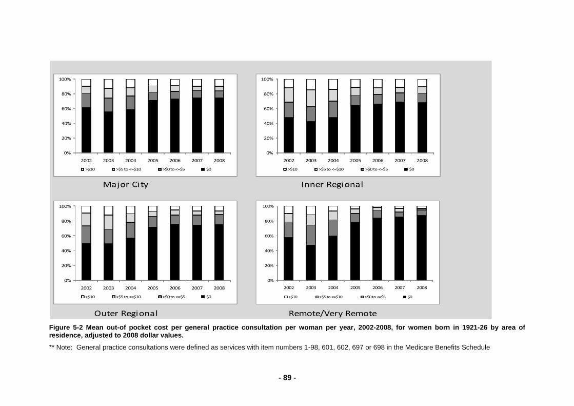
- 107 -
The mental health of the 1921-1926 cohort was also not significantly associated with any of the
environmental variables (Table 7-3). Similarly to the models for the other two cohorts, individual level
income management was the only statistically significant factor, where women who found it difficult to
manage on their income had poorer mental health outcomes.
Table 7-3 Regression models for mental health component scores in the 1921-1926 cohort: coefficients with confidence intervals that do not include zero are statistically significant.
1921-1926 Cohort : Mental Health Component Score, n=157
SALINITY
Coefficient (95% CI)
LST
Coefficient (95% CI)
NDVI
Coefficient (95% CI)
Environmental Variable -0.03 (-0.12, 0.06) -0.14 (-1.81, 1.44) 0.02 (-1.58, 1.68)
Income Management
(reference is ‗Difficult‘)
Not too bad
Easy
4.37 (0.53, 8.22)*
6.56 (2.63, 10.49)*
4.26 (0.39, 8.08)*
6.48 (2.53, 10.51)*
4.41 (0.46, 8.27)*
6.65 (2.59, 10.70)*
Education
(reference is ‗Yr 10 or less‘)
Year 12
Trade
University
-0.97 (-5.36, 3.51)
-0.30 (-4.88, 4.37)
3.58 (-2.53, 9.62)
-0.93 (-5.45, 3.58)
-0.46 (-5.10, 4.13)
3.66 (-2.57, 9.86)
-0.97 (-5.36, 3.53)
-0.60 (-5.22, 4.14)
3.72 (-2.25, 9.68)
*statistically significant at p<0.05.
In summary we did not find any association between dryland salinity, land surface temperature (LST),
normalised difference vegetation index (NDVI), a proxy for rainfall, and mental health scores of
women in south-west Western Australia. Area level measurements of dryland salinity may be poorly
estimated and therefore not as useful for individual health outcome analyses, however the more
readily available and variable environmental measures such as LST and NDVI should be investigated
further. Any effect of soil salinisation on human health may be difficult to determine independently of
socioeconomic factors. An alternative interpretation is that this study provides evidence that
economic assistance and other adaptation responses to adverse environmental conditions, may
mitigate the impacts of environmental degradation and climate change on human health in Australia.
7.4. Qualitative experience of drought
The deleterious impacts of drought can be seen in farming and rural communities, where life and the
health of the land are highly interconnected. For example, income, career, family and social aspects
of rural life are clearly tied to agricultural productivity, which is adversely affected by drought. Past
research suggests that financial hardship, changes in family responsibility, and physical stress all
occur in the context of drought (Anderson, 2007; Sartore, 2007; Bryant & Pini, 2009; McMichael,
2009). However, the results reported in Section 7.1 - Section 7.3 suggest that health might not be
associated with living in areas affected by drought and drying.
The current investigation aimed to examine the lived experience of drought for Australian women over
time by analysing qualitative data provided by the ALSWH 1946-51 and 1921-26 cohorts. The
ALSWH 1946-51 cohort qualitative data set includes over 13 700 comments spanning the last fifteen
years and the 1921-26 cohort includes over 18,400 comments. These texts are unstructured
responses to the final survey question, which asks, ―Have we missed anything?‖
- 108 -
The comments of 78 women in the 1946-51 cohort and 20 women in the 1921-26 cohort who wrote
about drought were included in this narrative analysis. The main themes that arose from the data are
described below.
7.4.1. Drought as a burden
Many of the women in this study wrote clearly about their struggle with the drought and the impact it
was having on their family and community.
“We’re in the drought area. My husband missed out and we didn’t get any assistance
[drought assistance from government], because I am working, if I will not work I can’t help my
kids at uni…that’s the main reason for my depression alone” (1946-51 cohort participant).
“We are a farming family so things change from day to day. So we have many ups and
downs. Drought has been our biggest burden and will take a lot of years to get on top of
again” (1946-51 cohort participant).
“This area has been severely drought affected for some years. There is considerable worry in
most people in the district” (1921-269 cohort participant).
“The current drought is affecting all farming families. So far we are coping well, but if it doesn’t
rain soon the effects on the whole family will be severe. I don’t think anyone understands
what’s happening out here” (1946-51 cohort participant).
The drought was viewed as an external force to be reckoned with and one that required hard work.
The women often wrote about their stresses resulting from over work or increased responsibility.
“I still work on our farm as husband and son have paid work off farm because of the five year
drought in this area, no water, rain, work, no crops, no income and more money goes out, you
can have what’s left – the debt!” (1946-51 cohort participant).
“…only see my house to fall into bed at night after long days mustering or feeding drought
stock” (1946-51 cohort participant).
“We are in drought therefore the load is far greater physically” (1946-51 cohort participant).
Living with drought was found to place great financial pressure on women and their families. Many
women began employment off-farm to supplement farm income; often this meant travelling kilometres
from the family home. The impact of the drought on finances is a complicated situation.
“Endured a debilitating drought which has almost ruined me financially” (1946-51 cohort
participant).
“The long drought has caused a decrease in income” (1921-26 cohort participant).
“We have had 3 years of drought and have had no income this year” (1946-51 cohort
participant).
“I still have to shoulder a lot of responsibility to keep giving us a living after struggling through
eight years of drought” (1921-269 cohort participant).
“Drought has almost crippled us, this is why I have gone back to some part time work, as a
matter of fact, I had to” (1946-51 cohort participant).
7.4.2. Ageing in drought
The long lasting nature of drought, apparent from the above comments, led to the observation by
many women that they experienced the effects of ageing (eg menopause) in the context of drought.
Drought was found to impact on women‘s ability to plan for the impacts of ageing, retirement,
employment, or their physical and mental health needs. The women wrote about how living in drought
had impacted their ability to age and retire in the ways they once thought they would. For some
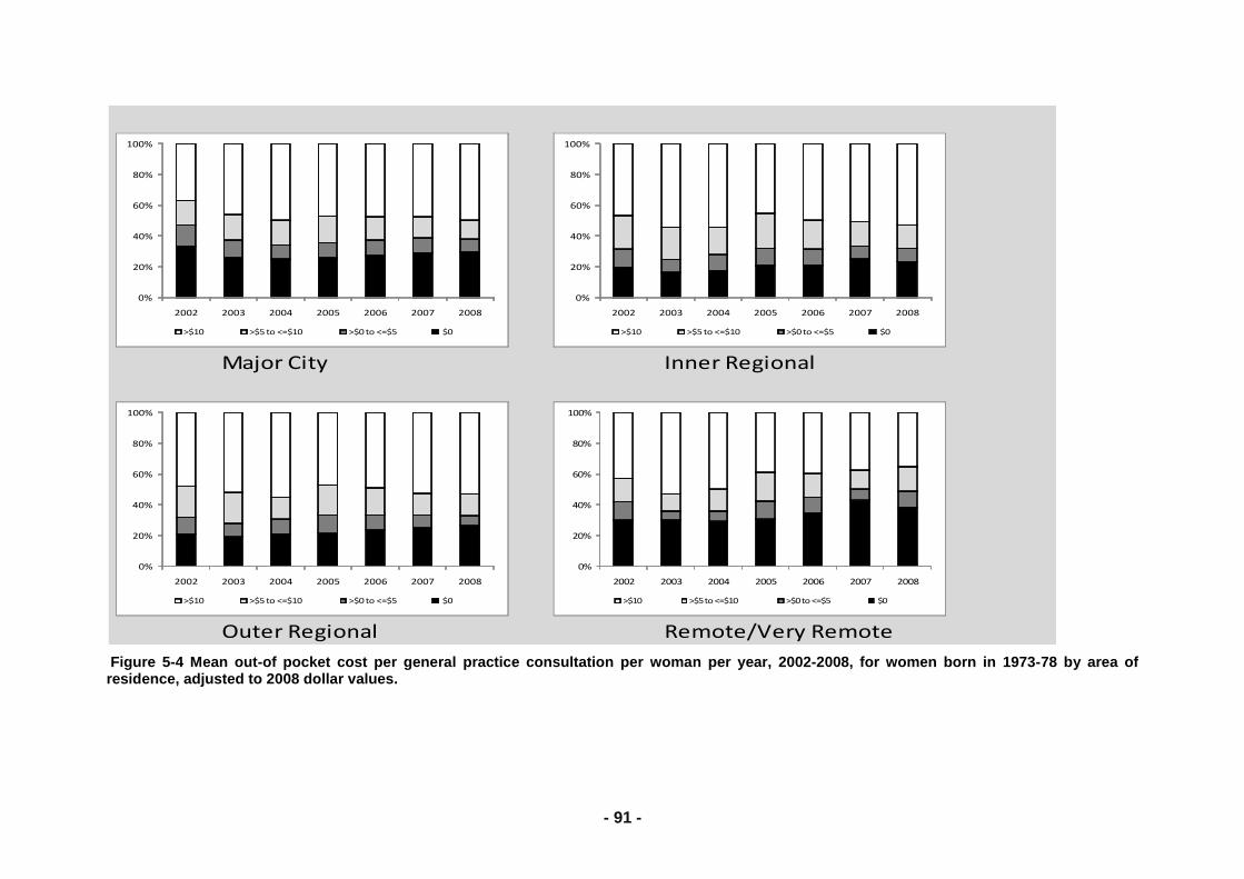
- 109 -
women, the drought has meant selling the farm. Drought was found to curtail women‘s freedom to
make financial decisions for the future. These narratives are significant in respect to healthy ageing.
“…when the drought breaks, then I will retire” (1921-26 cohort participant).
“Sometimes I feel trapped by this situation and know I must keep working” (1946-51 cohort participant).
“Own our own farm and with the drought lasting so long, retirement is looking a long way down the track” (1946-51 cohort participant).
“The last 3 years have been the most trying times I can remember in 51 years, drought and poor prices…too old to have paid employment” (1921-26 cohort participant).
“It is depressing to be sinking into debt at this age and see my husband work to no avail” (1946-51 cohort participant).
7.4.3. Resilience during drought
In the face of this adversity and uncertainty, however, women also reported undertaking proactive
and inventive approaches to enable them to manage their health, wellbeing, families and other
responsibilities. These adaptive strategies constitute the theme of resilience. Many women may have
wished for times when life on the farm was easier; however, their continued attempts to ease their
situation were overtly clear.
“Thinking positive…to not let the drought situation take over” (1946-51 cohort participant).
“I must stay well to cope [with drought]” (1946-51 cohort participant).
“Worst drought and times are very very bad- but so far so good. Hoping for rain very soon. My
motto is when times are tough the tough keep going (I hope and pray)” (1946-51 cohort
participant).
“The drought is a worry, but is out of man’s control, so have a good laugh” (1946-51 cohort
participant).
“5 years of drought and still not out of the woods yet, and now a collapse of the cattle market;
but we are still here” (1921-26 cohort participant).
7.4.4. Conclusion
The qualitative comments presented here highlight the varied experiences of drought. Despite the
obvious adverse impacts of drought on income, future planning, and wellbeing the women in this
investigation also demonstrated adaptive capacities that helped them to cope with drought. It is
possible that this type of resilience and adaptability assists in buffering adverse impacts of drought on
physical or mental health. Future research is needed to investigate these factors further, at the
population level. In particular, it will be important to identify those aspects of government policy, such
as exceptional circumstances assistance, that might build resilience at the personal and community
levels to offset the stress of climate events.
Those that are most affected by drought are those who also contribute to Australia‘s food production.
Providing the appropriate services and support mechanisms for people living with drought is an
essential element of responses to drought and climate change. Examining those strategies that have
already worked for people, as demonstrated in the current research, can help to inform service
development.
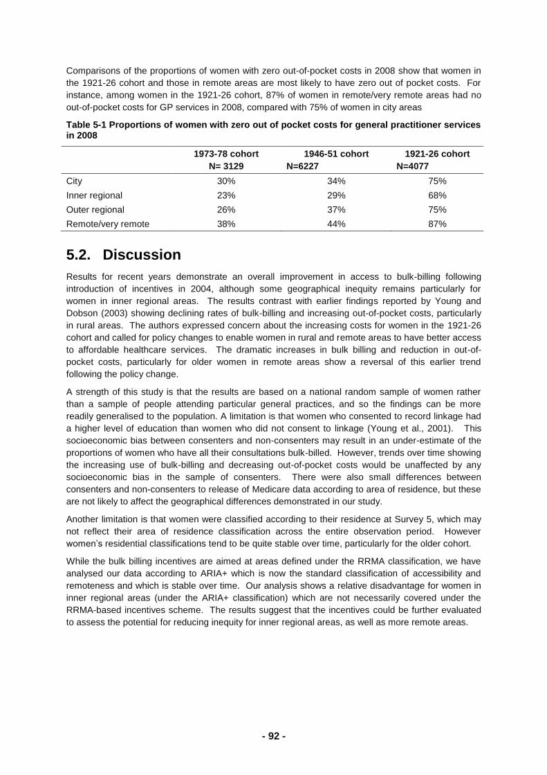
- 110 -
7.5. References
Anderson, D. (2007). Drought, Endurance and 'The way things were‘: The lived experience of climate
and climate change in the Mallee. Australian Humanities Review (45):67-81.
Bryant, L. & Pini, B. (2009). Gender, Class and Rurality: Australian Case Studies. Journal of Rural
Studies, 25: 48-57.
McMichael, A. (2009). Climate Change in Australia: Risk to Human Wellbeing and Health, Nautilus
Institute Australia (in partnership with RMIT University).
Sartore (2007). Drought and its effect on mental health. Australian Family Physician 36(12): 990-993.
Smith D, Hutchinson M, McArthur R. Climatic and Agricultural Drought: Payments and Policy.
Canberra, ACT: Centre for Resource and Environmental Studies, Australian National
University. 1992
- 111 -
8. Social cohesion
8.1. Neighbourhood
There is an extensive literature that ascribes protective benefits for both morbidity and mortality to the
presence of strong social support. Both the empirical literature and anecdotal evidence suggest that
rural communities are more socially cohesive than metropolitan communities, with rural communities
providing strong social support networks that are protective for their members‘ physical and
psychological well-being. Social support can be provided and received at both an individual and a
community level and community physical or social characteristics may exert their own effects on
individual health and behaviour in the same way that individual level characteristics of social support
can exert powerful effects on health and well being. Feeling part of a neighbourhood and being safe
within that neighbourhood both contribute to social engagement and enhanced well-being. Because
women from the 1946-51 birth cohort are the least likely to have changed residence in the previous
three years (Australian Bureau of Statistics, 2008), data from this cohort were used to explore
perceptions of neighbourhood, an important aspect of social cohesion. Questions about
neighbourhood were asked at Survey 3, when women were aged 47 to 52 years. Neighbourhood
data were available for 11,221 women.
8.1.1. Neighbourhood connection
Figure 8-1 shows the differences in neighbourhood connection scores of women in each geographic
location. A higher neighbourhood connection score reflects greater levels of interaction with
neighbours, involvement in local issues, perceptions of commonality with neighbours, and helpfulness
of people in the neighbourhood. There was a downward trend in neighbourhood connection scores
from remote/very remote areas, outer regional areas, inner regional areas, with women living in major
cities having the lowest neighbourhood connection scores. Women living in remote/very remote areas
had significantly higher neighbourhood connection scores than did women living in major cities.
Figure 8-1 Mean neighbourhood connection scores and 95% confidence intervals in each geographic location
18.40
18.60
18.80
19.00
19.20
19.40
19.60
19.80
20.00
20.20
20.40
20.60
20.80
Remote/very remote Outer regional Inner regional Major city
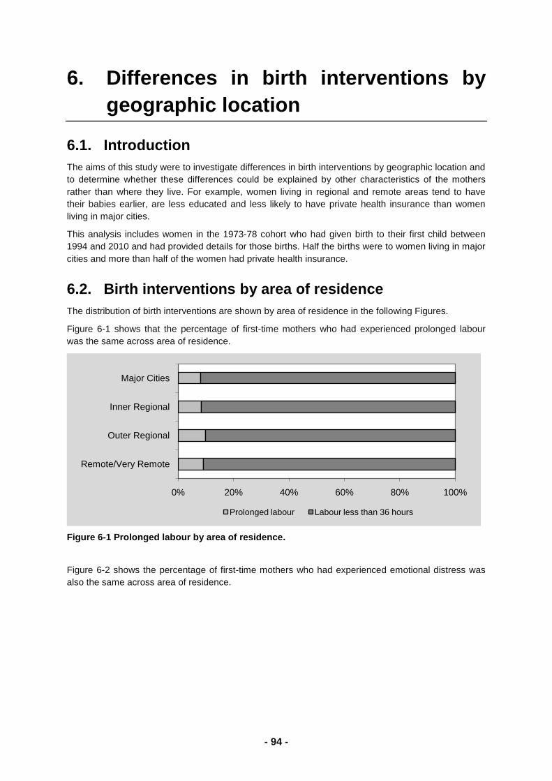
- 112 -
8.1.2. Neighbourhood safety
Neighbourhood safety was measured by asking the women if they believed that it was safe for
children to walk around the neighbourhood during the day, and if it was generally safe to walk at night
in the neighbourhood. Figure 8-2 shows the differences in neighbourhood safety scores of women in
each geographic location. Women living in remote/very remote areas had significantly higher
neighbourhood safety scores than did women living in major cities. There was a downward trend in
neighbourhood safety scores from remote/very remote areas, outer regional areas, inner regional
areas, with women living in major cities having the lowest neighbourhood safety scores.
Figure 8-2 Mean neighbourhood safety scores and 95% confidence intervals in each geographic location
7.00
7.20
7.40
7.60
7.80
8.00
Remote/very remote Outer regional Inner regional Major city
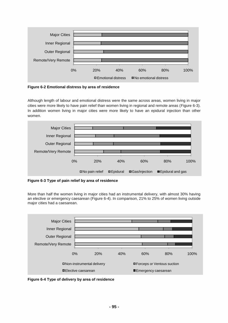
- 113 -
8.1.3. Neighbourhood attachment and trust
Figure 8-3 describes the differences in neighbourhood attachment and trust scores of women in each
geographic location. A higher neighbourhood attachment and trust score reflects liking and wanting
to stay in the neighbourhood, feeling respected, and trusting neighbours to look out for property.
Women living in inner regional areas had significantly higher neighbourhood attachment and trust
scores than did women living in major cities.
Figure 8-3 Mean neighbourhood attachment & trust scores and 95% confidence intervals location
18.80
19.00
19.20
19.40
19.60
19.80
Remote/very remote Outer regional Inner regional Major city
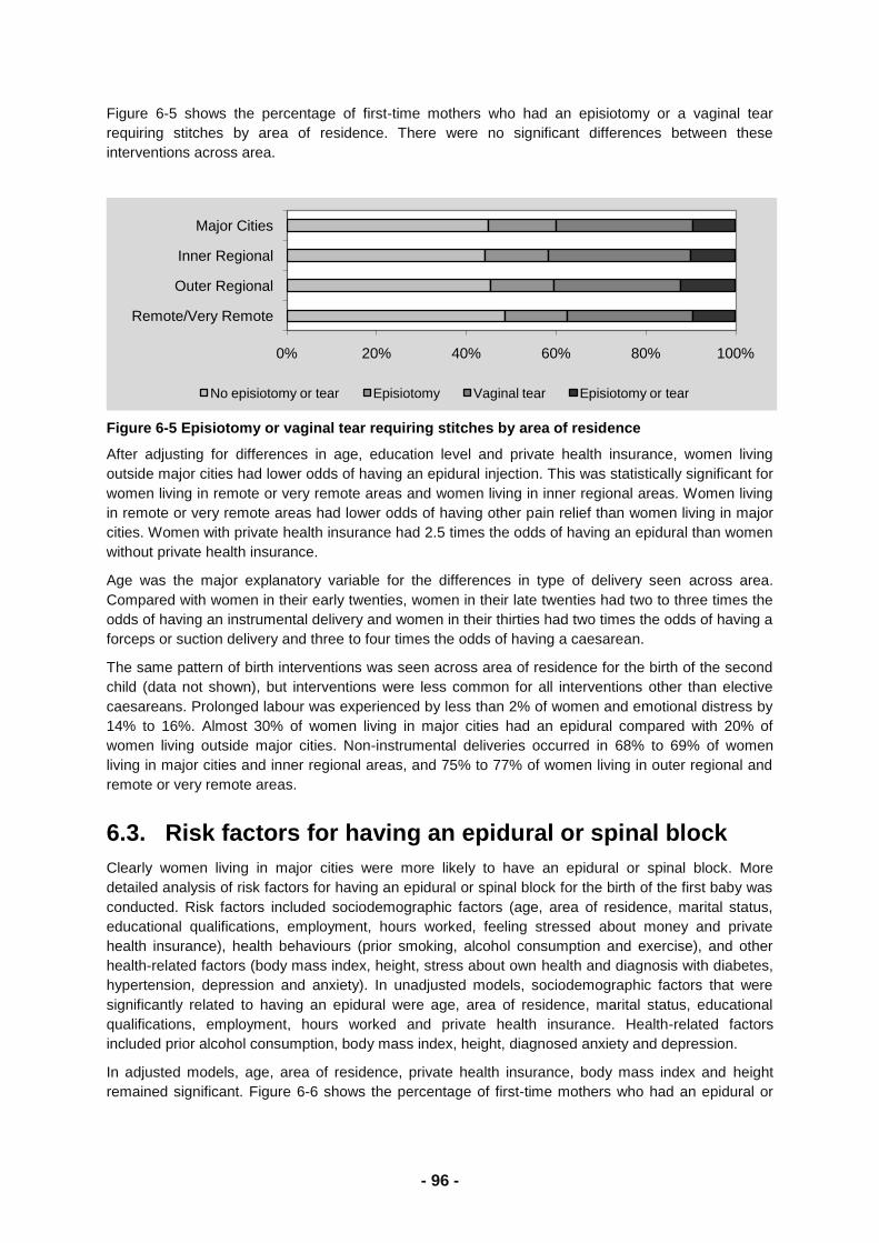
- 114 -
8.1.4. Social support
In addition to the community level support that was measured with perceptions of neighbourhood, we
also asked the women about personal social support, that is the availability of someone to offer
companionship and emotional and instrumental support. Figure 8-4 shows levels of social support
among women in each geographic location. Most women reported having access to social support
―all of the time‖. The patterns of access to social support were similar in each geographic area.
Figure 8-4 Proportion of women reporting level of social support in each geographic location
0 20 40 60 80 100
Remote/v remote
Outer regional
Inner regional
Major city
None, or a little of the time Some of the time Most of the time All of the time
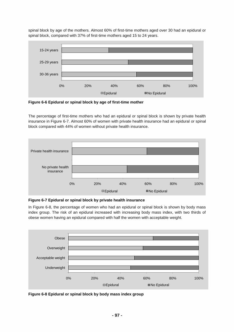
- 115 -
8.1.5. Life satisfaction
Figure 8-5 shows the differences in life satisfaction of women in each geographic location. The score
reflects how satisfied women are in relation to work, career, family relationships, study, friendships,
partner/closest personal relationship, and social activities. Higher scores indicate greater satisfaction
in life. Women living in remote/very remote areas had significantly higher life satisfaction scores than
women living in major cities.
Figure 8-5 Mean life satisfaction scores and 95% confidence intervals in each geographic location
3.00
3.02
3.04
3.06
3.08
3.10
3.12
3.14
3.16
3.18
Remote/very remote Outer regional Inner regional Major city
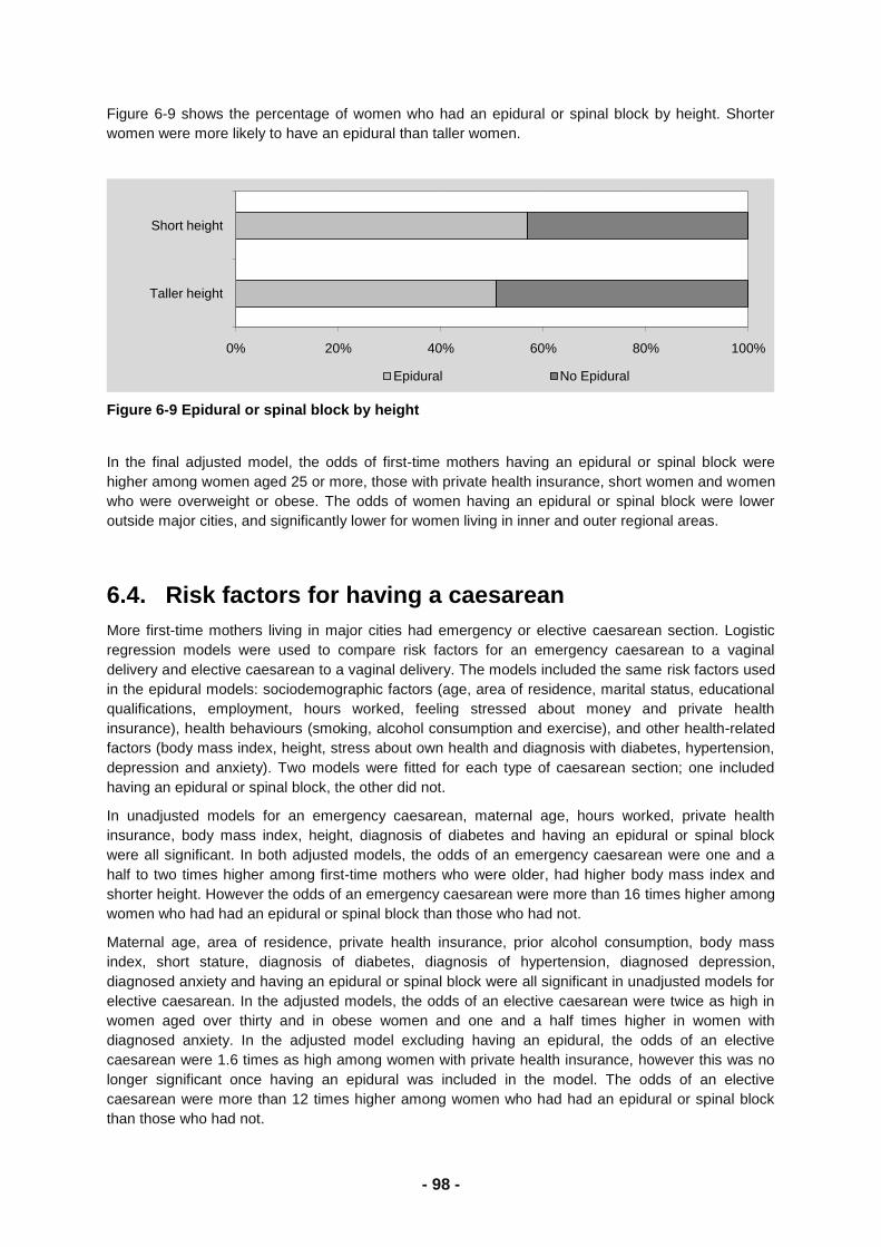
- 116 -
8.1.6. Stress
Figure 8-6 shows the perceived stress levels of women in each geographic location. Stress levels
relate to how stressed women reported being in relation to their own and family member health, work,
living arrangements, money, and relationships. Most women reported being ―somewhat stressed‖,
with significantly fewer women reporting being ―very stressed‖ and small numbers of women reporting
being ―not at all stressed‖. This pattern was similar in each geographic area.
Figure 8-6 Proportion of women reporting levels of stress in each geographic location
75 80 85 90 95 100
Remote/v remote
Outer regional
Inner regional
Major city
Not at all stressed Somewhat stressed Very stressed
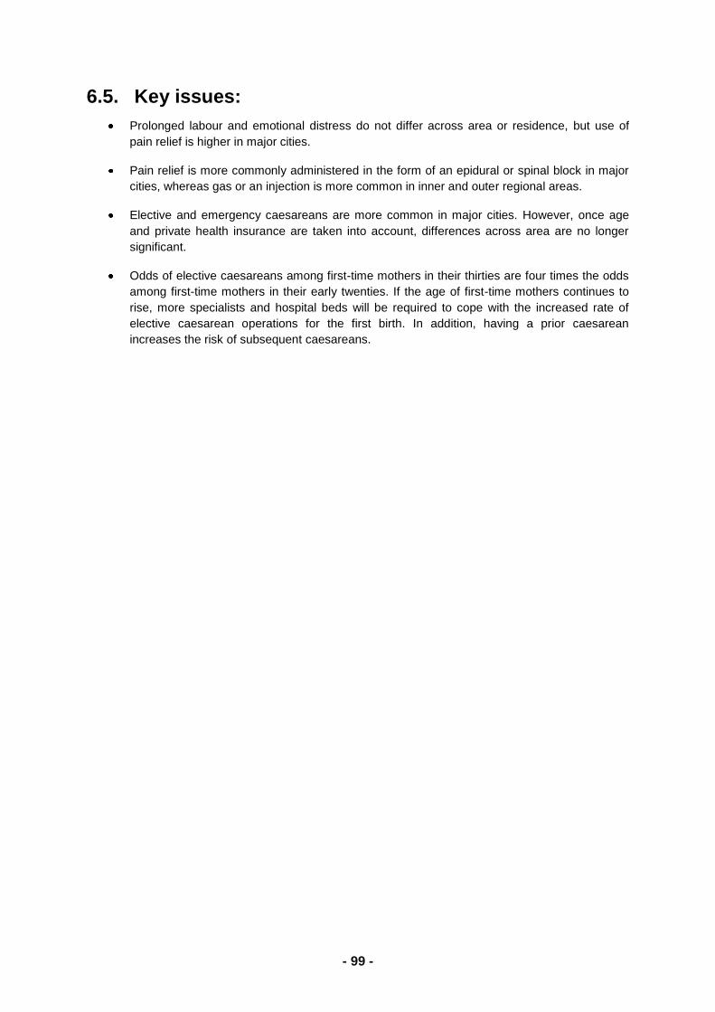
- 117 -
8.1.7. Perceived control
Figure 8-7 shows differences in the amount of control women perceive they generally have (eg. what
happens in most situations), and the extent to which they feel they are able to effect change. Higher
scores indicate perceptions of greater control.
Figure 8-7 Mean perceived life control scores and 95% confidence intervals in each geographic location
18.80
19.00
19.20
19.40
19.60
19.80
20.00
20.20
20.40
Remote/very remote Outer regional Inner regional Major city
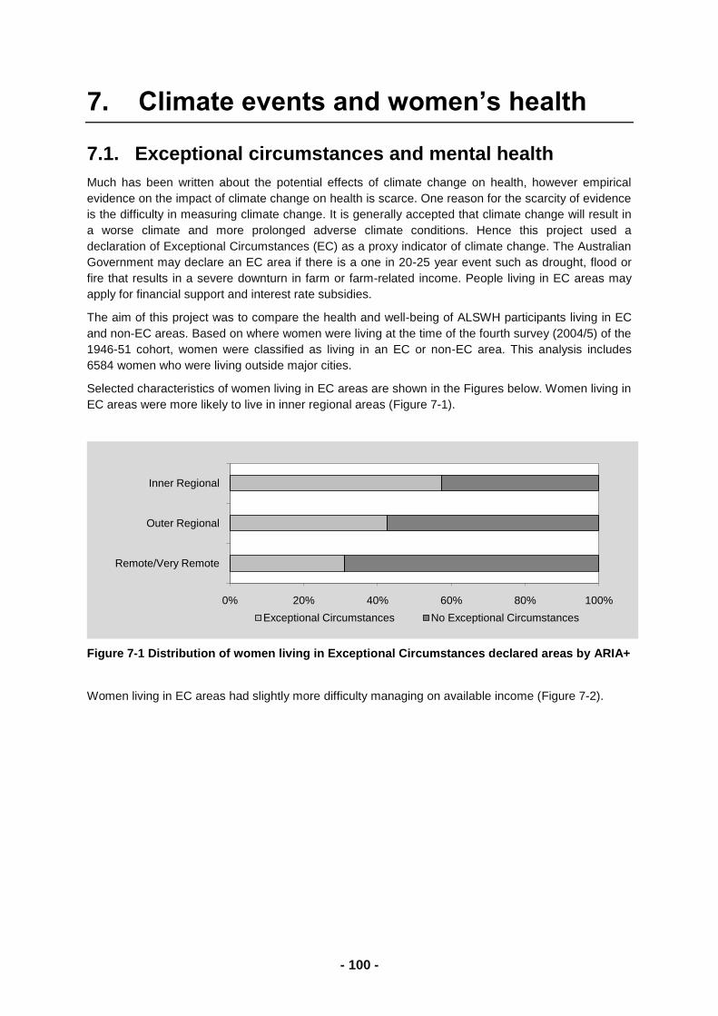
- 118 -
8.1.8. Optimism
Figure 8-8 shows differences in optimism scores of women across geographic areas. The optimism score reflects general expectations of positive or negative things happening to them.
Figure 8-8 Mean optimism scores and 95% confidence intervals in each geographic location
8.1.9. References
Australian Bureau of Statistics (2008) Residential and Workplace Mobility, and Implications for Travel:
NSW and Victoria, Canberra.
15
15.2
15.4
15.6
15.8
16
16.2
Remote/very remote Outer regional Inner regional Major city
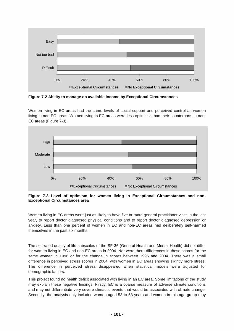
- 119 -
8.2. Cohesion/satisfaction
8.2.1. Introduction
It has been argued that rural residency may be a proxy indicator of a variety of health determinants
including socio-economic disadvantage, high-risk occupation, poor service access and exposure to
unfavourable environmental events (Smith, Humphreys & Wilson, 2008). For these reasons the health
of rural residents should be poorer than residents in metropolitan communities. It may be that social
support lessens or mediates the effects of rurality-based socio-economic disadvantage on health,
however, research on rural populations is sparse, and the direction of these relationships is currently
unclear.
We undertook a series of face to face interviews in 2010 with 13 rural women participants and 10
urban participants in the 1921-26 cohort and explored the role of social support on their well-being. An
analysis of the women‘s comments revealed seven major areas or themes describing the role of
social support in their lives. These themes are described below and illustrated with comments from
the women.
The first theme concerned access to social networks and how this can be difficult for older women,
especially because of driving and mobility limitations imposed by increasing age or the distances
involved in rural areas. Interview comments reflecting this included:
...the lady in the other unit, she said she’d take me. She’s been pretty good to me, that other lady over there. Then the dog had bitten her and she was in hospital, and I used to ride the scooter up to hospital every day.
She had someone that comes once a month that takes her out for three hours... I said look come over here next time. I said I’ll give you a cup of tea and something to eat or we can go to the pub and have lunch or whatever.
But at the same time I have been isolated,.... well if can’t drive that’s a problem.
The next theme reflected how life on a country property can be difficult for women, particularly during
the years they are raising their children. Many of the women in our study commented on the
loneliness that they experienced when they were younger, as these woman describe:
After we lost (our baby) I just went to pieces for a while. The doctor was really good, and again mum and dad were living just down the road. I always said I don’t know how I would have ever pulled through except for them.
I used to sit on the verandah at 6 o’clock at night and see the tractor going around and round, and think, what am I doing here?
It was lonely because see I only had brothers and we were out in the prickly pear country. I think there might have been one woman about 20 miles away somewhere.
Another theme focussed on the changes that occur as the women‘s children became older, and the
women were free to take up off-farm pursuits, such as joining country women‘s groups. The following
quotations describe how some women enjoyed these activities
I tell you, I really enjoyed those 10 years (as a group member) because on the farm you’d be by yourself all day.
We were in the CWA choir. And we had a ton of fun.
- 120 -
In another theme, a number of women commented that establishing and maintaining social networks
was easier for women than for men:
My opinion about life is that women can go out and get a lot of interesting things to do where a lot of men can’t.
He didn’t enjoy that either because he couldn’t assimilate with people a lot. ... all he knew was farming. He’d have to be talking to another farmer to understand it all.
....he wouldn’t join a club, the seniors’ club.
The next theme identified how in rural areas, neighbours are often the most frequently utilised
sources of social support:
My advice to my daughter when she got married, I said, go to your next door neighbour and say can you tell me how to do this? People like to tell you things. They’ll be a friend for life.
Our neighbours at the farm, well, we’ve been neighbours for 60-odd years, and we’re still in contact with each other.
I’ve got friends here. People who are friendly to me, will help me if I need help. Friends and neighbours around the same age.
A further theme highlighted the particular demands of rural life and how they interfere with the ability
to socialise. For many women, younger as well as older, off-farm income is necessary for survival, as
these quotes illustrate:
Say a nurse might work five days a week – she might work more – but when she comes home, she’s got to catch up. I know women out there that have subsidised the farm for years.
.....they subsidise the financial part of the farm. And I know some that have worked for years.
Finally, the women identified the issue of increasing age and how it may limit the ability of older
women to stay in their homes. They highlighted the relatively frequent occurrence for rural women to
have to relocate to a town or even to a larger city where they could be closer to family members.
What I notice, I go to the shopping centre and I know nobody. And you walk along the street and there’s nobody who says, G’day.
Nobody wants to leave. Now these friends that I’ve known ever since I’ve been here they’re getting to the stage where they shouldn’t be living here anymore.
We’re all getting into the same situation health wise. I’ve got a couple of younger ones (friends) who I’m sure would help out in emergencies. I mean I’ve lost my very best friend from over the road, she died of cancer. It’s nearly three years ago but it feels like yesterday because we were friends for 20 odd years.
The findings from this study emphasise the strength and importance of social support in rural areas
and provide context for the quantitative data in Section 8.1. The following section describes a
particular aspect, driving, that can affect social isolation in rural areas.
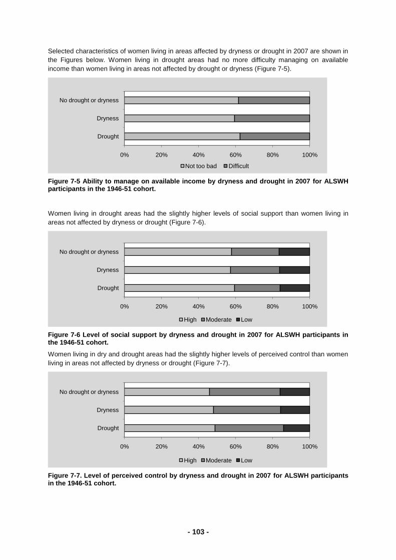
- 121 -
8.2.2. References
Letvak, S. (2002). The importance of social support for rural mental health. Issues in Mental Health
Nursing, 23, 249-261.
Smith, K.B., Humphreys, J.S. & Wilson, M.G. (2008). Addressing the health disadvantage of rural
populations: How does epidemiological evidence inform rural health policies and research?
Australian Journal of Rural Health, 16, 56-66.
Adams, M.H., Bowden, A.G., Humphrey, D.S. & McAdams, L.B. (2000). Social support and health
promotion lifestyles of rural women. Online Journal of Rural Nursing and Health Care 1,
Accessed at: http//www.rno.org/journals.
Gamarra, C.J., Paz, E.P. & Griep, R.H. (2009). Social support and cervical and breast cancer
screening in Argentinean women from a rural population. Public Health Nursing, 26, 269-276.
Baxter, J., Shetterly, S.M., Eby, C., Mason, L., Cortese, C.F. & Hamman, R.F. (1998). Social network
factors associated with perceived quality of life: The San Luis Valley health and aging study.
Journal of Aging and Health, 10, 287-310.
Chiu. H., Chen, C., Huang, C. & Mau, L. (2005). Depressive symptoms, chronic medical conditions
and functional status: A comparison of urban and rural elders in Taiwan. Journal of Geriatric
Psychiatry, 20, 635-644.
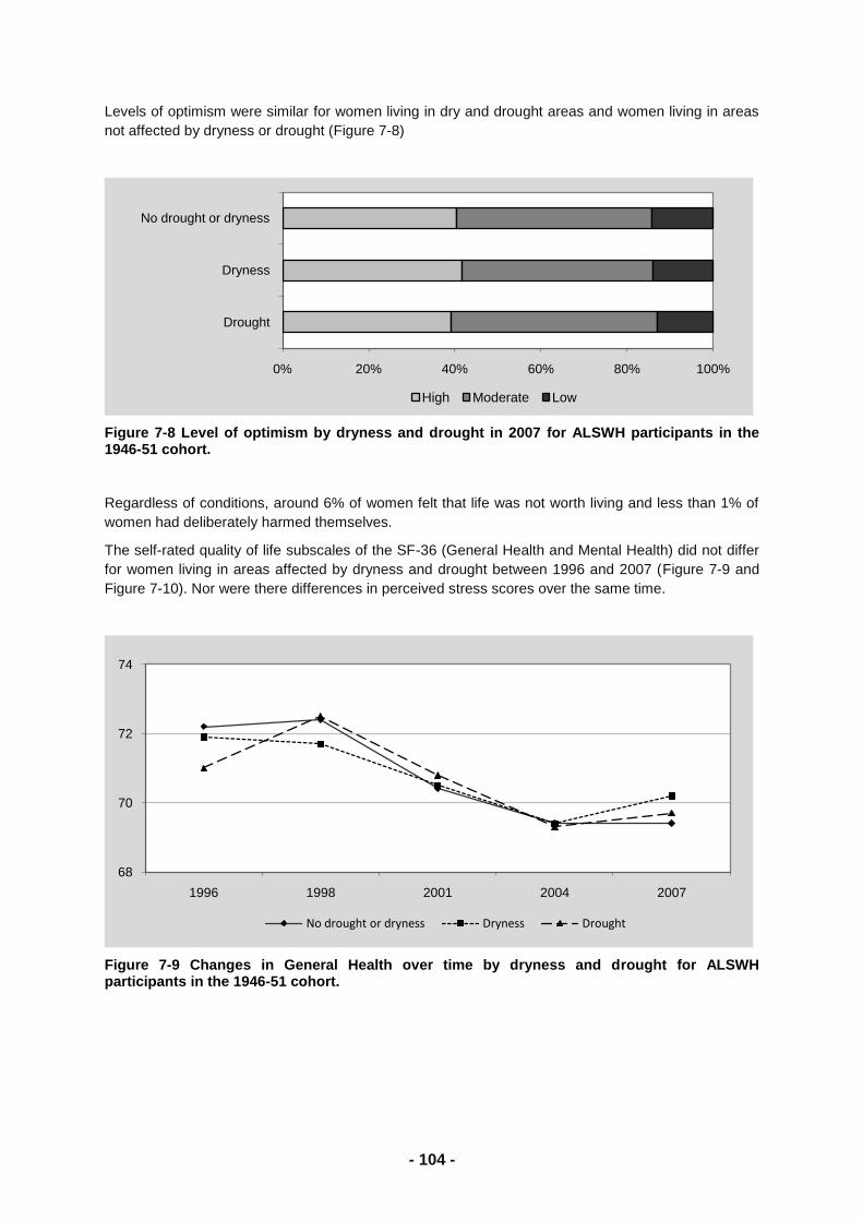
- 122 -
8.3. Driving
8.3.1. Introduction
The ability to drive is important for older peoples‘ mobility and social participation and may be the only
available means of transport and autonomy, especially for older people in rural areas (Murray, 1997).
Driving may also have another important social role for older women in allowing them to provide care
for others. However there are also many concerns with people‘s capacity and safety to keep driving
in old age (Dickerson, 2007). Older drivers have been shown to have high prevalence of conditions
such as vision and hearing impairment and musculoskeletal problems that can hinder driving abilities
(Anstey et al., 2006). Other chronic health conditions such as heart disease, diabetes and stroke
have also been associated with reduced driving ability (Dobbs & Carr, 2005) and drivers who have
cognitive impairment or dementia have been shown to have an increased risk of car accidents
(Anstey et al., 2006). Further, many drugs that are commonly used by older people (including
antihypertensives, ophthalmic agents, and analgesics) can have adverse effects on driving skills and
responses (Dobbs & Carr, 2005). Older drivers also have a proportionally higher risk of accidents per
kilometer driven when compared with younger age groups, although overall they account for a small
proportion of motor vehicle accidents (Tefft, 2008).
Many older drivers voluntarily reduce their driving, avoid driving at night or in rain, or cease driving
altogether (D‘Onorfio et al., 2008), or they may be forced to give up their driving licence following an
assessment of their fitness to drive. However, many older adults are very unwilling to make the
decision to stop driving, and regret the decision once it is made (Johnson, 2008).
Among the older ALWH cohort, driving is the main form of transport, especially for women in rural and
remote areas (Byles et al., 2007). In this section of the report we describe trends in the proportion of
older women who drive themselves as their main means of transport, and factors associated with
giving up driving – particularly for women in regional and remote areas who may have fewer transport
options, and for women who have a caregiving responsibility.
8.3.2. Main means of transport
We first asked about main means of transport at Survey 3 when the women were aged 76-81 years.
At that time, 55% of the women were driving themselves as their main means of transport. Three
years later, at Survey 4, 86% of these women were still driving themselves, and 73% were still driving
themselves at Survey 5 (when they were aged 82-87 years). After accounting for other factors that
affect driving (see below), women were 20% less likely to be driving at Survey 4 compared to Survey
3 and 38% less likely to be driving at Survey 5. The majority of women who did not drive themselves
relied on another driver for their main means of transport with very few women using taxis or other
public transport.
There was a strong and statistically significant association between main means of transport and area
of residence at all surveys. At each survey there was a decline in the proportions of women who were
driving themselves as the main means of transport in all areas, an increase in the proportion driven by
someone else, a slight increase in the use of taxis, and a reduction in the use of other forms of
transport (see Figure 8-9).
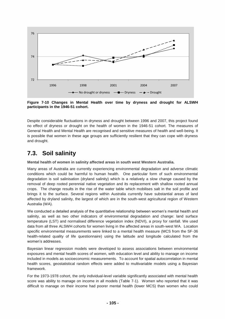
- 123 -
Figure 8-9 Main means of transport for women in major cities, regional, and remote areas at Survey 3 (N= 7966), Survey 4 (N=6197) and Survey 5 (N=4772)
8.3.3. Factors associated with continuing to drive
On longitudinal analyses a number of factors were associated with driving.
The effect of area was such that, after accounting for time and compared to major cities, the odds of
driving were 52% higher in inner regional areas, 110% higher in outer regional, and 117% higher in
remote areas. Women were less likely to continue driving if they reported diabetes, stroke, vision
problems, and need for help with daily tasks. Higher SF-36 Physical Function scores were associated
with continuing to drive.
Compared to women with no caring role, women who cared for someone who lived with them were
32% more likely to drive, and women who cared for someone who lived elsewhere were 69% more
likely to drive. Likewise, women who were single, divorced or widowed were 38% more likely to drive
than married women, and women with higher levels of education were more likely to drive than those
who did not complete school.
0%
10%
20%
30%
40%
50%
60%
70%
80%
90%
100%
Car (you drive) Car (someone else drives) Taxi Bus Tram or train
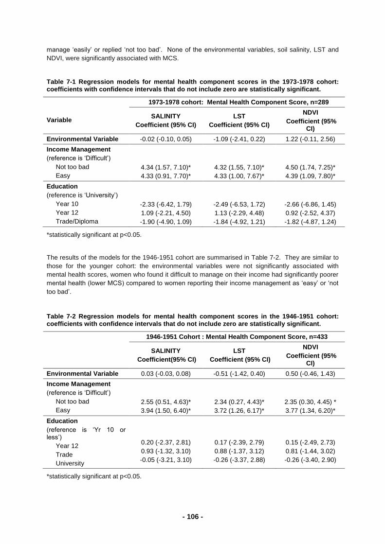
- 124 -
Table 8-1 Factors affecting odds of driving, over time and across areas
Factor Odds Ratios (95% Confidence Intervals)
Intercept 0.31 (0.27-0.36)
Time
Survey 3 (ref) 1
Survey 4 0.81 (0.78-0.84)
Survey 5 0.66 (0.63-0.70)
ARIA classification
Major City (ref) 1
Inner regional 1.59 (1.45-1.75)
Outer regional 2.26 (2.00-2.55)
Remote 2.17 (1.57-2.99)
Health conditions*
Hypertension NS
Diabetes 0.80 (0.72-0.89)
Stroke 0.66 (0.56-0.78)
Vision problems* 0.72 (0.67-0.78)
SF-36 Physical Function** 1.01 (1.01-1.01)
Need for help with daily tasks* 0.50 (0.45-0.55)
Caregiving for someone who:*
lives elsewhere 1.73 (1.61-1.85)
lives with you 1.47 (1.35-1.59)
Marital Status Married/Defacto (ref) 1
Single 1.40 (1.30-1.51)
Education
No Qualifications (ref) 1
School/intermediate certificate 1.50 (1.35-1.67)
Higher school/leaving certificate 1.74 (1.51-2.01)
Trade 1.33 (1.04-1.69)
College or University 2.56 (2.22-2.95)
*Reference level is not having condition
** Continuous variable
8.3.4. Discussion
This study provides a significant amount of information about older women drivers across urban
regional and remote areas. The majority of women aged 76-81 years (at Survey 3) who reported
driving as their main means of transport were still driving themselves when re-surveyed three and six
years later. The study suggests that a majority of older women will maintain driving while ever their
health will allow it, and particularly if they are living in regional or remote areas, not married, or if they
have caring responsibilities. Women were less likely to drive if they reported conditions such as
diabetes and stroke and if they had physical limitations or poor vision. This association with vision
has been reported in other research (eg. Anstey et al., 2006; Ross et al., 2009) and it is estimated
that vision accounts for 95% of driving capability (Laux & Brelsford, 1990). Women themselves also
highlight the importance of good vision for maintaining driving (Byles et al., 2007; Ragland et al.,
2004).
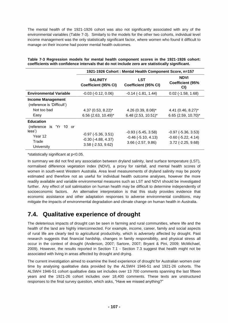
- 125 -
In general, women are less likely to drive at older ages than men are. In one study of people aged 65
and over, men were 5.7 times more likely to drive than women and were more likely to drive with
significant physical, sensory or cognitive disability (Ross et al., 2009). However, despite their lower
probability of driving and therefore their lower overall crash rate (Bayam et al., 2005), older women
have been found to be disproportionately represented in fatal accidents occurring in low traffic and
low risk conditions (Baker et al., 2003). These findings suggest that even though women are more
likely to drive in regional and remote areas than in urban areas, the quieter traffic conditions may not
protect them from risk or hazard. Indeed in one study, rural older drivers were less likely to adhere to
stop signs than urban drivers (Keay et al., 2009) suggesting rural drivers may take more risks
(Rakauskas et al., 2009).
However, women in regional and remote areas may have few alternatives to driving. In this study,
women were unlikely to use public transport alternatives, even in urban areas. For these older
women, driving is essential to their social participation, and to access health care and other services,
particularly if they do not have a husband or someone else who can drive for them (Johnson, 2008;
Byles et al., 2009). Women who had caring responsibilities were particularly likely to be driving at
older ages. The ability of these women to drive to get around is important therefore, not only for their
own sakes, but in allowing them to contribute to the care of other possibly frail older people.
The issue of older women drivers is therefore a complex consideration of not only fitness to drive but
also the social needs and benefits of their driving, and the availability of acceptable alternatives
(Dickerson et al., 2007). As Oxley et al., (2010) note, ―responses to the older driver problem should
be multi-scalar‖, and should include vehicle and road design, alternative transport options and
supportive infrastructures, effective licensing systems, and driver education/training tools.
This study is limited in that it relies on self-reported driving and does not have data on licensing,
driving behaviour or accident history. It is probable that the women who continued driving had altered
their driving behaviour as they aged in terms of the distances travelled and the conditions they drive
under. The study is also unable to report on the driving status of those women who failed to respond
to the surveys and who may have been more frail.
These analyses show that older women in more rural and remote areas, women who are no longer
married, and women who have caring responsibilities are more likely to drive than urban women. For
these women, driving remains an important factor for their ongoing participation and contribution to
society. There is a need for greater understanding of how we can respond to the changing needs of
older women who need to continue to drive despite age and physical limitations, as well as
considering the implications for road safety.
8.3.5. References
Anstey KJ, Windsor TD, Luszcz MA & Andrews GR. (2006). Predicting driving cessation over 5 years
in older adults: psychological well-being and cognitive competence are stronger predictors than
physical health. Journal of the American Geriatric Society, 54(1):121-6.
Baker TK, Falb T, Voas R, Lacey S. (2003). Older women drivers: fatal crashes in good conditions.
Journal of Safety Research, 34(4):399-406.
Bayam E, Liebowotz J, & Agresti W. (2005). Older drivers and accidents: A meta-analysis and data
mining application on traffic accident data. Expert Systems and Applications, 29(3):598-629.
Byles J, Gibson R, Parkinson L, & Dobson A. ( 2009). Driving myself: Main forms of transport among
older women in rural and remote Australia. Intouch, Outback
Byles J, Gibson R, Parkinson L, & Dobson A. (2007). Driving myself: Main forms of transport among
older women in rural and remote Australia.
http://9thnrhc.ruralhealth.org.au/program/docs/papers/byles_A5.pdf
- 126 -
Dickerson AE, Molnar LJ, Eby DW, Adler G, Bedard M, Berg-Weger M, Classen S, Foley D, Horowitz
A, Kerschner H, Page O, Silverstein NM, Staplin L, & Trujilllo L. (2007). Transportation and
Ageing: A research agenda for advancing safe mobility. The Gerontologist, 47(5):578-590
Dobbs BM & Carr D.(2005). Screening and assessment of medically at-risk drivers. Public Policy and
Ageing Report, 15:6-12.
Donorfio LKM, D'Ambrosio LA, Coughlin JF, & Mohyde M. (2008). Health, safety, self-regulation and
the older driver: It‘s not just a matter of age. Journal of Safety Research, 39: 555-561.
Johnson JE. (2008). Informal Social Support Networks and the Maintenance of Voluntary Driving
Cessation By Older Rural Women. Journal of Community Health Nursing, 25:65–72.
Keay L, Jasti S, Munoz B, Turano KA, Munro CA, Duncan DD, Baldwin K, Bandeen-Roche KJ, Gower
EW, & West SK. (2009). Urban and rural differences in older driver‘s failure to stop at stop
signs. Accident Analysis and Prevention, 41:995-1000.
Laux LF & Brelsford J. (1990). Age-related changes in sensory, cognitive, psychomotor and physical
functioning and driving performance in drivers aged 40 to 92. Washington, D. C.: AAA
Foundation for Traffic Safety.
Murray SL. (1997). What's happening: Driving and the elderly. Journal of the American Academy of
Nurse Practitioners, 9(3), 133–136.
Ragland DR, Satariano WA &MacLeod KE. (2004). Reasons given by older people for limitation or
avoidance of driving. The Gerontologist, 44 (2): 237-244.
Rakauskas ME, Ward NJ, & Gerberich SG. (2009). Identification of differences between rural and
urban safety cultures. Accident Analysis and Prevention, 41: 931–937
Ross LA, Anstey KJ, Kiely K, Windsor TD, Byles JE, Luszcz MA, & Mitchell P. (2009). Older drivers in
Australia: Trends in Driving status and cognitive and visual impairment. Journal of the
American Geriatrics Society,57(10); 1868-1873.
Tefft BC. (2008). Risks older drivers pose to themselves and to other road users. Journal of Safety
Research, 39:577-582
www.alswh.org.au