Rural Labour Market Developments, Agricultural ... Labour Market Developments, Agricultural Productivity, and Real Wages in Bangladesh, 1950–2006 ... The focus of this paper is developments

The Pakistan Development Review 47 : 1 (Spring 2008) pp. 89–114

Rural Labour Market Developments, Agricultural Productivity, and Real Wages in Bangladesh,

1950–2006

AKHAND AKHTAR HOSSAIN*

This paper provides an overview of recent developments in rural labour markets in

Bangladesh and also examines the trends and movements of agricultural productivity and real wages with annual data for the period 1950–2006. The paper links the movements of agricultural real wages to macroeconomic developments in general and agricultural development in particular. As part of empirical investigation, the paper develops a simple model of agricultural real wages that depend on agricultural productivity. In order to examine the long-run relationship between agricultural productivity and real wages, the paper applies the Autoregressive Distributed Lag Bounds testing approach. Empirical results suggest that there exists a long-run relationship between agricultural productivity and real wages, and that agricultural productivity can be treated as a ‘long-run forcing variable’ in explaining agricultural real wages. In the dynamic specification of real wages, the coefficient on one-period lagged error-correction term bears the expected negative sign and is significant. The forecasting ability of the error correction model is satisfactory with respect to the level or the percentage change of real wages. The overall results are consistent with the findings of earlier studies that agricultural productivity is a key determinant of real wages in Bangladesh.

JEL classification: C32, J43, O13 Keywords: Rural Labour Markets, Agricultural Wages, Agricultural Productivity,

ARDL Bounds Testing Approach, Bangladesh

I. INTRODUCTION

After remaining relatively stagnant over the 1950s through the 1970s, the Bangladesh economy has been growing steadily since the 1980s at a rate of about 5 percent per annum. Foreign capital flows in the form of workers’ remittances, foreign aid and loans, and foreign investment have contributed to modern economic growth, which in turn caused a structural transformation of the economy in favour of the non-farm and services sectors [Hossain (2006)]. Consequently, labour markets have undergone a structural change in terms of employment and work patterns.1 Therefore the structural change in the labour markets represents a structural transformation of the economy especially since the 1980s. This did not however lead to the expected rush of workers to the urban areas. The significant improvement in the agricultural terms of trade since the beginning of economic deregulation in the mid-1980s, inherent rigidities in urban

Akhand Akhtar Hossain <[email protected]> is Associate Professor of Economics and Head of Economics Discipline, School of Economics, Politics and Tourism, Faculty of Business and Law, University of Newcastle, Australia.

Author’s Note: The author acknowledges the comments and suggestions received from two anonymous referees of this journal on an earlier draft. Any remaining shortcomings of this paper are the author’s responsibility.

1The distribution of employment indicates that agriculture employed about 80 percent of the total labour force in the 1950s and 1960s [Hossain (1995)]. Since the early-1980s the share of agriculture in employment has declined steadily. Agriculture’s share in employment in recent years was about 58 percent [Hossain (2007)].

Akhand Akhtar Hossain 90

(formal) labour markets and the increasing urban pollution and environmental problems appear to have slowed the shift of labour from agriculture to manufacturing and services. Nevertheless the structural change in labour and work patterns has been reflected in a number of ways. These include the associated labour mobility from the rural to the urban areas, between the farm and non-farm activities2 within the rural areas, between the formal and informal activities within the urban areas and from both the rural and urban areas to overseas destinations for employment and migration. Additional changes in the labour markets have included the rise in the participation of women and the productivity and wage differentials across sectors [Hossain (2007)]. With such developments, the economy has lately moved to a higher growth path exhibiting considerable dynamism, although the Lewisian3 turning point in the rural labour market (which may lead to a sharp rise in real wages) is yet to be witnessed. The focus of this paper is developments in the rural labour markets and the trends and movements of agricultural productivity and real wages4 since the 1950s given that they provide information on poverty, welfare and market forces in the rural labour markets within a deregulated, open economy setup.

The remainder of this paper is organised as follows. Section II reviews the changing rural employment and work patterns and discusses the movements of agricultural productivity and real wages since the early 1950s. Section III provides economic explanations for the movements of agricultural real wages since the 1950s by linking them to macroeconomic developments in general and agricultural development in particular. Section IV develops a simple model of agricultural real wages that depend on agricultural productivity. Section V examines the long-run relationship between

2For lack of consensus on various terminologies used to define employment and economic activity in

poor countries, this paper uses the convention of including in the non-farm category those activities that are not directly related to the production, distribution and marketing of agricultural products. Therefore, in addition to rural off-farm activities, non-farm activity includes the urban informal sector activity such as street selling and petty retailing, repair and other personal services, crafts and other manufacturing, construction work and non-mechanised form of transport, such as rickshaws. In the rural areas, non-farm (off-farm) activities include construction work, wood and bamboo crafts, fishing, rural transport, small-scale manufacturing, petty trading and personal services [Amin (1981); Hossain (1996)]. The wage rates for farm and non-farm activities may differ but are generally interdependent.

3According to the Lewis model, the real wage rate in the labour surplus rural sector remains constant and well below (say, about 30 percent) the industrial sector real wage rate. The industrial sector can therefore increase employment by drawing workers from the rural sector without raising the rural wage rate. It is only when the surplus labour in the rural sector is eliminated through industrialisation that there could be a rise in rural real wages. The main criticism of this approach to development is that if the size of surplus labour in the rural sector remains large and the industrial sector does not grow rapidly and raise the demand for labour (given the capital-intensive nature of its production), rural real wages may not rise much unless there is an increase in agricultural productivity that would determine the supply price of labour for the rest of the economy [ADB (2005); Todaro and Smith (2003)].

4Given the availability of data, this paper defines agricultural productivity as agricultural output at constant prices per cropped acreage, expressed in an index. Agricultural productivity is therefore equivalent to land productivity (or yield) and also represents total factor productivity given that land, labour and capital have a stable relationship, especially in traditional agriculture [Sen (1960)]. Agricultural real wages are defined as the average of the daily wage rates in Rupee/Taka (without food or payments in kind) over 12 months across regions of Bangladesh, expressed in an index and deflated by the cost of living index for rural households. In general, agricultural wages represent the wage rates for rural workers engaged in farm activities. Given the aggregation of data over time and regions, they do not capture the regional and seasonal variations of wages but represent the general trends over time for the country as a whole. The data appendix reports the data sources and the estimation methods of agricultural productivity and real wages.

Rural Labour Market and Real Wages 91

agricultural productivity and real wages by the Autoregressive Distributed Lag bounds testing approach. An associated short-run error-correction model is also estimated and used for forecasting both the level and the percentage change of real wages. Section VI summarises the results and draws conclusion. The paper has an appendix, which reports the data sources and the unit root tests results of variables deployed for the regression analysis.

II. CHANGES IN RURAL EMPLOYMENT AND WORK PATTERNS

Until the mid-1980s most rural workers in Bangladesh worked in the farm sector, especially in the crop sector. There were only limited non-farm activities available as a source of gainful employment. The situation has changed significantly since the mid-1980s. The agricultural sector has become diversified and workers remain engaged in both farm and non-farm activities. Similar changes have taken place in the urban areas. Traditionally the urban labour market was male-dominated and not many women were in the labour force. The scope of employment in the informal sector was limited. This has changed significantly, especially since opening up the economy in the early-1980s. An increasing number of female workers now work in the newly emerging industries in the private sector, such as the garment industry and various construction and retail trade activities. Many rural workers are therefore able to divide their time between the rural and urban activities, which include construction, petty trade and services. Such switch from rural to urban activities remains conditional on the relative availability of work in the rural and urban areas given that there are seasonalities in both the rural and urban activities. For example, rural farm activities are heavily concentrated during the plantation and harvesting seasons, while the urban construction activities increase sharply during the dry seasons. The entry of rural workers into urban sector activities is relatively easy given the informal nature of job contracts and the availability of replacement with a short notice. The remainder of this section provides an overview of changes in work patterns in the rural labour markets.

Farm Mechanisation and Employment: Agriculture in Bangladesh remains a small-scale family-based farming operation. The agricultural technology is traditional and only since the mid-1970s the agricultural sector has undergone change by adopting the seed-fertiliser-irrigation technology. Since the late-1970s farmers have started small-scale mechanisation of activities in the areas of cultivation, plantation, processing and distribution [Hossain (1988)]. The process has accelerated since the mid-1990s. For most farm activities, small-scale mechanised tools and implements are now widely used. There are a number of interrelated factors behind the increasing demand for mechanised farm tools and implements, including the shortages of draught power, the availability of imported cheap tools, the availability of electricity in villages, the consideration of low time-requirement for cultivation and the utilisation of mechanised tools for alternative income-generating activities [Alam, Rahman, and Mandal (2004)]. Farmers who need credits for the purchase of farm machineries are able to borrow subsidised loans from publicly owned agricultural banks. A large number of non-government organisations also provide small-scale loans to rural borrowers for investment purposes. Contrary to expectations, the increased farm mechanisation (along with infrastructural and technological developments) has created employment opportunities for otherwise low-skilled workers while the most enterprising and skilled farm workers have opted for more


remunerating non-farm activities in both the rural and urban areas. With increasing farm mechanisation the women labourers’ involvement in both farm and non-farm activities has increased significantly.

Expansion of Non-farm Activities: According to a study by Hossain, Bose, Chowdhury and Meimzen-Dick (2002), the relative importance of agriculture as a source of employment for the rural workforce has decreased significantly over the past two decades. For example, only 14 percent of the rural land-poor households depended on agriculture for their employment in 2000 while this rate was 31 percent in 1988. Income from rural non-farm activities has also grown at a significantly faster rate than agricultural income during 1987–2000. About 40 percent of the rural labour force is presently engaged in rural non-farm activities. These include construction, retail trade and business, transportation and professional services [Ahmed and Sattar (2004)]. The increasing importance and potential for rapid growth of the rural non-farm sector has lately been recognised by the World Bank (2003).

Livestock and Poultry Rearing: As indicated earlier, until the 1970s the crop sector dominated agriculture. It is only since the early 1990s the livestock sector has become important in terms of its contribution to output and employment. Presently this sector contributes about 10 percent of the value added in agriculture and about 3 percent of GDP. Leather and leather products also contribute significantly to exports. This sub-sector remains labour-intensive and provides employment for about 20 percent of the population.

Export-Oriented Shrimp Sector: Since the economy opened up in the early-1980s, Bangladesh has developed an export-oriented fishing industry. This activity grew at a record pace in the 1990s, driven by the export-oriented shrimp production. Fisheries doubled its share in agriculture value added during the 1990s and accounted for nearly a quarter of total value added in agriculture in 2001 [World Bank (2003)]. The favourable exchange rates, trade incentives and the liberalisation of imports (that allowed duty-free inputs for commercial fish farming) helped the rapid growth of this sector. In the coastal areas, shrimp farming has become the most profitable economic activity. In fact in the mid-1990s Bangladesh accounted for about 4.4 percent of the global production of commercial shrimps. After garments, the shrimp sector has lately become the second largest export industry in the country. As shrimp-farming remains labour-intensive, this sector employs over half a million rural poor in various stages of processing and shrimp culture. This sector also employs a large number of female workers in both upstream and downstream activities, such as services, transport, catching of shrimp fries, and shrimp processing [Ahmed and Sattar (2004)].

Summing Up: The rural economy of Bangladesh has diversified over the past two decades and this has created considerable employment opportunities for both skilled and unskilled workers in farming and non-farming activities. Given the informal nature of employment contracts, the switch from farm to non-farm activities remains relatively easy and this has helped rural workers who lately devote a considerable amount of time to gainful non-farm activities. The increase of employment opportunities in non-farm activities explains why there has been absorption of the incremental labour force in the rural economy. Given few wage-rigidities, employment has increased at a steady pace while real wages have increased at a relatively slow pace. This fits well with the


Lewisian model [Lewis (1954); Todaro and Smith (2003)] of unlimited supply of labour in the rural sector. However it was not the industrial sector but the non-farm activities in both the rural and urban areas that provided most employment for the incremental labour force. The industrial sector did not exhibit expected dynamism. Likewise, the agricultural sector faces a number of growth-inhibiting constraints such as controls over output pricing and marketing, less export orientation and the slowdown of demand for agricultural products, especially food crops that have a lower than one income elasticity of demand [Ahmed and Sattar (2004); Abdullah and Shahabuddin (1997)].

III. REAL WAGES IN BANGLADESH’S AGRICULTURE: TRENDS AND MOVEMENTS

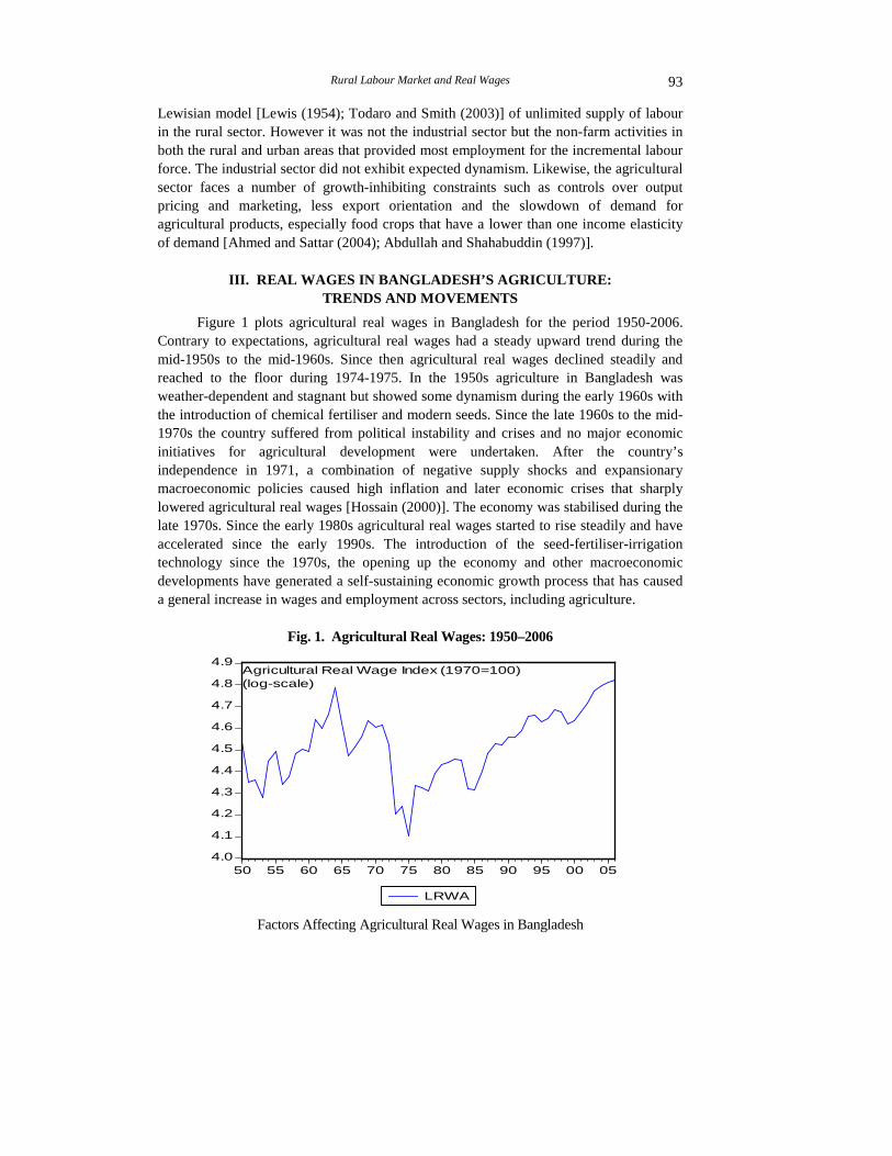
Figure 1 plots agricultural real wages in Bangladesh for the period 1950-2006. Contrary to expectations, agricultural real wages had a steady upward trend during the mid-1950s to the mid-1960s. Since then agricultural real wages declined steadily and reached to the floor during 1974-1975. In the 1950s agriculture in Bangladesh was weather-dependent and stagnant but showed some dynamism during the early 1960s with the introduction of chemical fertiliser and modern seeds. Since the late 1960s to the mid-1970s the country suffered from political instability and crises and no major economic initiatives for agricultural development were undertaken. After the country’s independence in 1971, a combination of negative supply shocks and expansionary macroeconomic policies caused high inflation and later economic crises that sharply lowered agricultural real wages [Hossain (2000)]. The economy was stabilised during the late 1970s. Since the early 1980s agricultural real wages started to rise steadily and have accelerated since the early 1990s. The introduction of the seed-fertiliser-irrigation technology since the 1970s, the opening up the economy and other macroeconomic developments have generated a self-sustaining economic growth process that has caused a general increase in wages and employment across sectors, including agriculture.

Fig. 1. Agricultural Real Wages: 1950–2006

4.0

4.1

4.2

4.3

4.4

4.5

4.6

4.7

4.8

4.9

50 55 60 65 70 75 80 85 90 95 00 05

LRWA

Agricultural Real Wage Index (1970=100)(log-scale)

Factors Affecting Agricultural Real Wages in Bangladesh


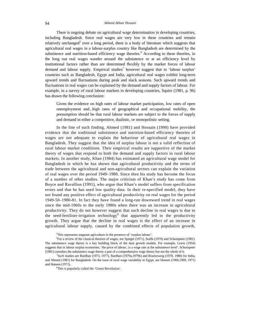
There is ongoing debate on agricultural wage determination in developing countries, including Bangladesh. Since real wages are very low in these countries and remain relatively unchanged5 over a long period, there is a body of literature which suggests that agricultural real wages in a labour-surplus country like Bangladesh are determined by the subsistence and nutrition-based efficiency wage theories.6 According to these theories, in the long run real wages wander around the subsistence or at an efficiency level by institutional factors rather than are determined flexibly by the market forces of labour demand and labour supply. Empirical studies7 however suggest that in ‘labour surplus’ countries such as Bangladesh, Egypt and India, agricultural real wages exhibit long-term upward trends and fluctuations during peak and slack seasons. Such upward trends and fluctuations in real wages can be explained by the demand and supply factors of labour. For example, in a survey of rural labour markets in developing countries, Squire (1981, p. 96) has drawn the following conclusion:

Given the evidence on high rates of labour market participation, low rates of open unemployment and...high rates of geographical and occupational mobility, the presumption should be that rural labour markets are subject to the forces of supply and demand in either a competitive, dualistic, or monopolistic setting.

In the line of such finding, Ahmed (1981) and Hossain (1990) have provided evidence that the traditional subsistence and nutrition-based efficiency theories of wages are not adequate to explain the behaviour of agricultural real wages in Bangladesh. They suggest that the idea of surplus labour is not a valid reflection of rural labour market conditions. Their empirical results are supportive of the market theory of wages that respond to both the demand and supply factors in rural labour markets. In another study, Khan (1984) has estimated an agricultural wage model for Bangladesh in which he has shown that agricultural productivity and the terms of trade between the agricultural and non-agricultural sectors can explain the variation of real wages over the period 1949–1980. Since then his study has become the focus of a number of other studies. The major criticism of Khan’s study has come from Boyce and Ravallion (1991), who argue that Khan’s model suffers from specification errors and that he has used low quality data. In their re-specified model, they have not found any positive effect of agricultural productivity on real wages for the period 1949-50–1980-81. In fact they have found a long-run downward trend in real wages since the mid-1960s to the early 1980s when there was an increase in agricultural productivity. They do not however suggest that such decline in real wages is due to the seed-fertiliser-irrigation technology8 that apparently led to the productivity growth. They argue that the decline in real wages is the effect of an increase in agricultural labour supply, caused by the combined effects of population growth,

5This represents stagnant agriculture in the presence of ‘surplus labour’. 6For a review of the classical theories of wages, see Spiegel (1971), Sraffa (1970) and Schumpeter (1981).

The subsistence wage theory is a key building block of the dual growth models. For example, Lewis (1954) suggests that in labour surplus economies, ‘the price of labour...is a wage rate at the subsistence level’. Schumpeter (1981) considers the subsistence wage theory a part of a comprehensive wage theory but not the whole of it.

7Such studies are Bardhan (1973, 1977), Bardhan (1979a,1979b) and Rosenzweig (1978, 1980) for India, and Ahmed (1981) for Bangladesh. On the issue of rural wage variability in Egypt, see Hansen (1966,1969, 1971) and Hanson (1971).

8This is popularly called the ‘Green Revolution’.


rising landlessness and insufficient economic growth in non-farm sectors. Palmer-Jones (1993) has criticised the Boyce-Ravallion study. He has shown that their model fails the prediction and stability tests when it is estimated with an expanded data set up to 1989. By including a dummy for 1972–1974 and a discontinuous time trend with a value one for the period 1949–1964 and zero afterward, he has come to the conclusion against the Boyce-Ravallion finding. In a rebuttal, Ravallion (1994) has acknowledged the prediction failure of their model but criticised Palmer-Jones’s use of dummies and the time trend. He stands by the view that agricultural real wages in Bangladesh were declining much of the 1960s and 1970s. Palmer-Jones (2004) has not conceded but maintains his view against any declining trend in real wages in Bangladesh.

While the above studies have kept the issue in agricultural wage determination alive, they remain exposed to criticisms. First, all these studies probably use non-stationary data and therefore the regression results reported may not be robust, if not spurious. Provided that the variables of interest have a unit root, the cointegration-error correction approach may provide better results. An error-correction model is also useful to investigate the dynamic behaviour of real wages. Secondly, some of the earlier studies focused on responses of agricultural nominal wages to commodity prices, although in a theoretically consistent, parsimonious wage model the focus should be real wages. Theoretically, a wage determination model does not make much sense when agricultural nominal wages are linked to the prices of rice, jute and cloth because all these prices move together and are determined simultaneously by say an exogenously determined policy variable—the money supply. In a long-run wage model, real wages should be determined by real factors such as agricultural (or labour) productivity. Rashid (2002) has updated earlier studies and used the cointegration approach to determine the relationships among agricultural wages, rice prices, urban wages and so on. Although he has adopted a sound statistical approach, he has fallen in the same trap of examining the responses of nominal wages to a set of commodity prices. He did not examine the linkage between agricultural real wages, productivity and other variables of interest that may explain the growth of agricultural real wages.

As pointed out earlier, there have been major changes in Bangladesh’s agriculture since the 1950s. Agricultural real wages have exhibited upward trends and sharp fluctuations over time. Rather than determined institutionally, there are reasons to believe that the long-term real wages in Bangladesh agriculture remain linked to agricultural productivity.9 This proposition can be established analytically in a broader context of agricultural wage determination in developing countries.

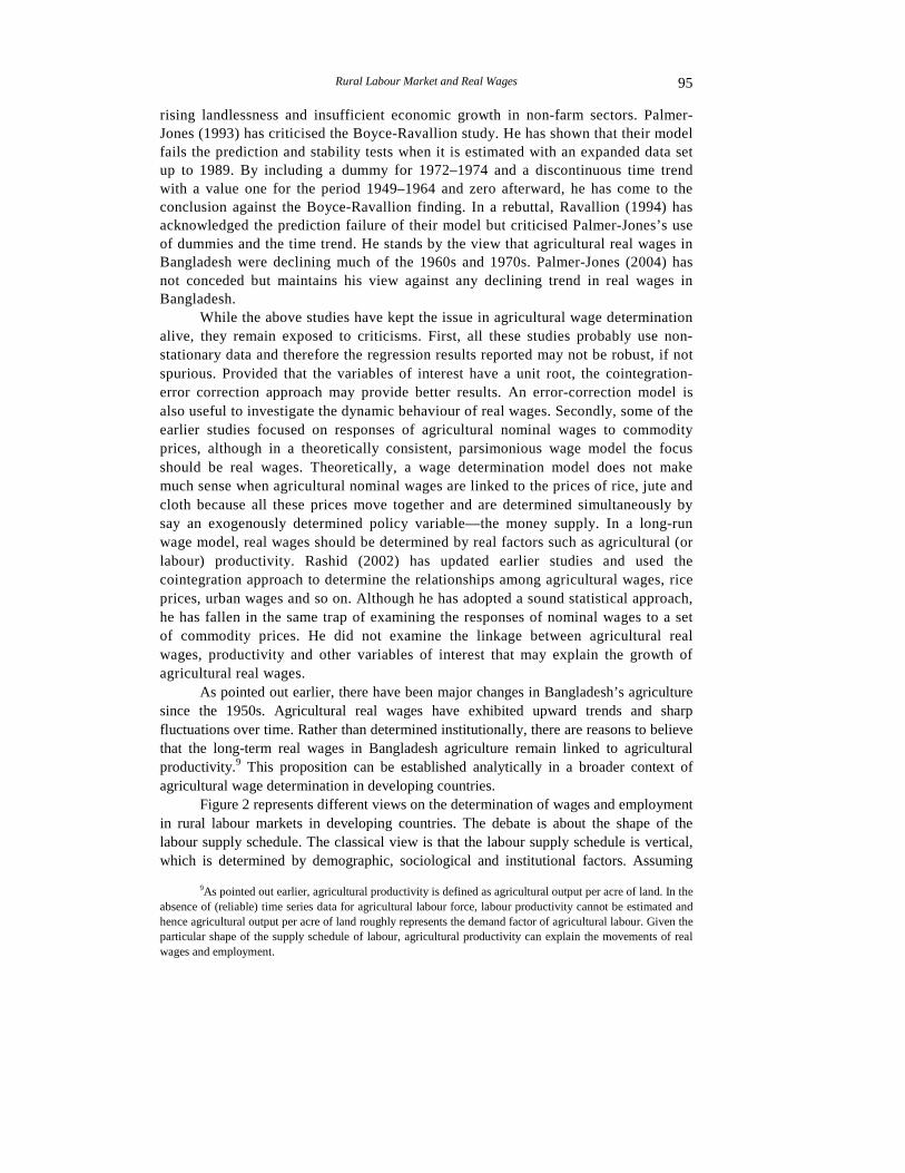
Figure 2 represents different views on the determination of wages and employment in rural labour markets in developing countries. The debate is about the shape of the labour supply schedule. The classical view is that the labour supply schedule is vertical, which is determined by demographic, sociological and institutional factors. Assuming

9As pointed out earlier, agricultural productivity is defined as agricultural output per acre of land. In the absence of (reliable) time series data for agricultural labour force, labour productivity cannot be estimated and hence agricultural output per acre of land roughly represents the demand factor of agricultural labour. Given the particular shape of the supply schedule of labour, agricultural productivity can explain the movements of real wages and employment.


that the supply schedule of labour is vertical,10 real wages fluctuate between w2 and w1 in response to a shift in demand for labour and thereby full-employment is maintained. In contrast, the Keynesian/structuralist supply curve of labour is horizontal say at the subsistence wage level (ws) and a shift in the demand for labour changes the level of employment between E2 and E1. Unlike the classical case of full-employment, the Keynesian/structuralist horizontal supply curve of labour predicts unemployment when there is a downward shift in the demand for labour because real wages remain inflexible downwards on subsistence and efficiency grounds. The standard Lewisian rural labour market with surplus labour [Lewis (1954)] also assumes a horizontal supply curve of labour at the subsistence wage rate ws until the level of employment reaches the Lewisian turning point (E2) when a further increase in the demand for labour raises real wages given the upward sloping segment of the labour supply schedule. Thus, in short, the different models of rural labour markets provide different implications for changes in real wages and employment from any shift in the demand for labour. The classical/neoclassical model predicts fluctuations of real wages in response to any shift in demand or supply schedule of labour or both while full-employment is maintained. The Keynesian/structuralist model predicts fluctuations of employment in response to a shift in the demand for labour while real wages remain stable at the subsistence level. In the Lewis model, real wages remain stable until the surplus labour is exhausted. Although the neoclassical model predicts fluctuations of wages and employment, it can explain a relatively stable real wages over time when a rightward shift in the demand for labour schedule matches a rightward shift in the supply schedule of labour.

Fig. 2. Agricultural Real Wages and Employment

10Empirical studies suggest that the agricultural labour supply schedule in a developing country like Bangladesh is positively sloped rather than perfectly elastic. For example, based on a large-scale employment and unemployment survey of households in West Bengal, Bardhan (1979a, p.73) has concluded: ‘my evidence seems to be against the standard horizontal supply curve of labour assumed in a large part of the development literature’. His estimated wage elasticity of the supply of labour is roughly between 0.2 and 0.3 for casual farm workers and small farmers, which is certainly very low compared with the infinite elasticity presumed in the horizontal supply curve of agricultural labour.

SL (classical)

SL (neoclassical)

SL (Keynesian/ Structuralist)

Real Wage (w)

D0 D1

w2

Ws

D2

w1

SL (Lewisian)

Employment Ef E1 E2


One stylised fact of the rural labour markets in Bangladesh is the very low rate of (open) unemployment, say, about 3 percent of the labour force. Given that the rural workers are very poor11 and there are no well-developed social-security arrangements, the poor workers simply cannot afford to remain unemployed. Those who remain unemployed may not be actively in the labour force or may prefer to remain unemployed because most of them come from relatively rich households and keep themselves occupied with non-farm activities.

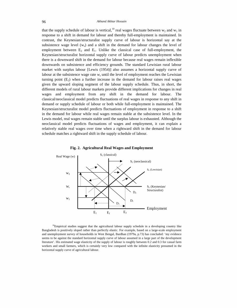
This paper maintains that agricultural real wages in Bangladesh are flexible and can be explained within the classical/neoclassical labour market paradigm. Although the agricultural sector was relatively stagnant during the 1950s and early 1960s, the introduction of the seed-fertiliser-irrigation technology since the late 1960s has raised agricultural productivity.12 Various income generating activities in the non-farm sectors have also affected the supply of labour in farm activities. However the sharp fluctuations of real wages reflect various shocks to the economy, especially in the 1960s and 1970s. Figure 3 plots agricultural productivity over the period 1950–2006. It reveals that agricultural productivity has increased steadily since the mid-1950s and that there is a distinct upward trend since the late 1980s.

Fig. 3. Agricultural Output Per Cropped Acreage: 1950–2006

4.2

4.4

4.6

4.8

5.0

5.2

5.4

50 55 60 65 70 75 80 85 90 95 00 05

LAQ

Agricultural Output Per Cropped Acreage Index(1970=100) (log-scale)

11Most rural workers come from landless households and they hold only limited productive assets. 12This paper does not investigate the factors that affect agricultural productivity. However the view that

the seed-fertiliser-irrigation technology is linked to agricultural productivity is well-established [Hossain (1996)].

LAQ


IV. AGRICULTURAL WAGE DETERMINATION MODEL

This section specifies a simple model of agricultural real wages. The model is specified in accordance with the market theory of the demand for and supply of labour. Assume that agricultural production in Bangladesh takes a Cobb-Douglas13 form:

Q = Q(L; A) … … … … … … … (1)

where Q is agricultural output per acre of land, L is the variable input labour per acre of land and A is the technological parameter. In this production function, capital is not included on the assumption that it bears a fixed relationship with land, especially in traditional agriculture [Sen (1960)]. A shift in technology represents the introduction of say modern technology and/or opening up the economy for foreign trade and investment.

Let w be the real wage rate in agriculture. Assuming that agricultural output is exogenously determined, the restricted cost function is given by

C = C(w; Q) … … … … … … … (2)

For a given Cobb-Douglas production function (1), the restricted cost function can be expressed, following Varian (1984), as:

C = Q wα … … … … … … … … (3)

where α ≤1. This cost function is popularly called the Cobb-Douglas cost function [McFadden

(1978)]. The partial derivative of the restricted cost function with respect to the wage rate yields the labour demand function. From Equation (3) the derived demand for labour Ld is given by:

Ld = δC/δw = Q α wα –1 … … … … … … (4)

In a logarithm form, the labour demand equation can be expressed as:14

ln Ldt = ln α + ln Qt + (α–1) ln wt … … … … … (5)

where t is the time subscript. Equation (5) suggests that the demand for labour is a decreasing function of the real wage rate unless α takes the value one.

Assume that the supply of labour Ls is an increasing function of the real wage rate. On the assumption of a constant elasticity, the log-linear labour supply schedule can be expressed as:

ln Lst = ln β0 + β1 ln wt … … … … … … (6)

13Shahabuddin (1985), using farm level data, has found that the Cobb-Douglas restrictions are validated

against both transcendental and translog functions for aman rice, pulses, wheat, oilseeds and boro rice, but not in case of aus rice and jute. For aus rice, the translog function gives a better fit, but for jute, the test results are inconclusive. In an aggregative production function (and in the yield equation), the Cobb-Douglas functional form seems a reasonable approximation.

14It is expected that the labour demand and labour supply relations are inherently non-linear. A log-linear form is postulated because such a transformation facilitates estimation and the estimated coefficients can be interpreted as elasticities. Moreover, logarithmic forms are almost exclusively employed in the literature on labour market analysis [Rosen and Quandt (1978)].


The equilibrium real wage rate we is assumed to be determined by the demand for and supply of labour. Equating the demand and supply equations for labour, the following reduced form wage equation is obtained as:

ln wet = δ0 + δ1 ln Qt … … … … … … (7)

where δ0 = ln α–ln β0/β1–(α–1) and δ1 = 1/β1–(α–1). Given that the values of β1 and α are positive, the term δ1 = β1–(α–1) is positive. This suggests that, given a negatively sloped demand for labour schedule, agricultural real wages respond to productivity depending on the slope of the supply curve. If β1 ≅ ∝ (the horizontal labour supply schedule), an increase in productivity (Q) (say because of the adoption of the new seed-fertiliser-irrigation technology and/or opening up the economy) would not increase real wages but only employment. On the other hand, if β1 is positive (the neoclassical labour supply schedule), an increase in productivity would increase both real wages and employment. In case β1 = 0 (the classical vertical labour supply schedule), an increase in productivity would increase only real wages but no employment. In short, the model developed above suggests that agricultural real wages are determined by the demand and supply functions of labour, which, in the absence of any institutional constraints, would yield a perfectly competitive market outcome. When there are institutional wage fixing arrangements, the equilibrium real wages may however not coincide with a perfectly competitive market outcome [Lewis and Kirby (1987)]. It is possible that there may also be a lag in the adjustment of the actual wage rate to the equilibrium wage rate. If there is any discrepancy between the equilibrium wage rate and the actual wage rate due to shocks, the actual wage rate may move towards the equilibrium wage rate through say a partial adjustment mechanism, such that

ln wt – ln wt–1 = γ (ln wet – ln wt–1) + ut … … … … (8)

where γ is the coefficient of adjustment, whose value is expected to lie between zero and one. When γ equals 1, the labour market is in full equilibrium, adjusting instantly to exogenous changes in the demand for and supply of labour. When γ = 0, real wages are independent of the demand and supply factors of labour. If the actual real wage rate adjusts only partially towards its equilibrium value, the model can be classified as a disequilibrium model [Lewis and Makepeace (1984)]. The error term (u) takes into account any random factors that may affect real wages.

Substitution of Equation (7) into Equation (8), and rearrangement of terms, yields the following partial-adjustment model:

ln wt = γ δ0 + γδ1 Qt + (1–γ) ln wt–1 + ut … … … … (9)

The above dynamic model of the agricultural wage rate is in full agreement with the laws of demand and supply. While excess demand in the labour market acts as a trigger for a wage increase, the model shows that the actual magnitude of wage increase depends on such parameters as the wage elasticities of the demand for and supply of labour and the speed of wage adjustment. At equilibrium, wt = wt–1 = we

t. In short, the competitive model of wage adjustment predicts wage changes by combining three factors: the extent of stock disequilibrium in the labour market, the elasticities of the demand for and supply of labour, and the speed of wage adjustment in response to disequilibrium in the labour market.


V. AGRICULTURAL PRODUCTIVITY AND REAL WAGES: AN EMPIRICAL INVESTIGATION

Estimation of a long-run relationship between agricultural productivity and real wages involves testing for the presence of a cointegral relationship between them. As part of empirical investigation, the time series properties of these variables are investigated by both the ADF and the KPSS tests over the sample period 1950-2006. The data appendix reports the results. They suggest that both these series have a unit root. However the Perron test, which takes into account the structural break in 1972,15 suggests that these series do not have a unit root. Such conflicting results are common in applied work given the low power of unit root tests. For the present purposes, there is a choice with respect to the appropriate procedure for estimation of a long-run relationship between agricultural productivity and real wages. In the literature, the two most commonly used approaches to testing for the long-run relationships between variables in levels are the Engle-Granger two-step residual based procedure [Engle and Granger (1987)] and the Johansen’s system-based reduced rank regression approach [Johansen (1988); Johansen and Juselius (1990)]. These approaches involve the cases where all the underlying variables are integrated of order one. As most applied researchers face the problem of not knowing with certainty that the variables in the relationship under investigation have a unit root, there is a growing literature that uses the autoregressive distributed lag (ARDL) cointegration approach. The ARDL cointegration approach has been developed in a series of papers by Pesaran and Shin (1996), Pesaran and Pesaran (1997), Pesaran and Smith (1998) and Pesaran, Shin and Smith (2001), which remains valid irrespective of whether the regressors are purely I(0), purely I(1) or mutually cointegrated. Although this approach does not require pre-testing for unit root in the series before testing for the long-run relationship, any information gained from testing for a unit root in the series may become useful for making inference when the calculated F-statistic falls inside the critical value bounds. In addition to the conflicting unit root test results, there are practical advantages of the bounds test. First, the ARDL approach is statistically superior to the Johansen approach when the sample size is small. The Johansen approach in particular is highly sensitive to choices made with respect to the intercepts and trends and the lag length in the variables. Secondly, the ARDL approach allows for distinguishing between jointly determined and ‘long-run forcing variables’, which may become useful for the interpretation of results based on theoretical insights.

Having considered these factors, this paper applies the ARDL bounds testing approach to determine the relationship between agricultural productivity and real wages in Bangladesh. The testing procedure is described first, which is followed by the empirical results. The ARDL Modeling Approach

Following Pesaran and Pesaran (1997), an error-correction version of the ARDL model in the generic variables y and x is given by

∆yt = α0 + α1Trend + Σβi ∆yt–i + Σφi ∆xt–i + δ1 yt–1 + δ2 x t–1 (i = 1, 2, 3….p) … (10)

15The country became independent in December 1971. The Perron test takes this exogenous event into

account while examining the time series properties. The data appendix reports the procedure and the results obtained by the Perron test.


where the coefficients βi and φi represent the short-run dynamics of the underlying variables in the ARDL model and the coefficients δs represent the long-run relationship. The underlying null hypothesis that there is no long-run relationship (implying no cointegration) between y and x is an F-test for the restriction that H0: δ1 = δ2 = 0 against the alternative that H1: δ1 ≠ 0, δ2 ≠ 0. The model is estimated first in a restricted form by excluding the level form lag variables and then test for the significance of the lagged level variables through variable addition test.

Accordingly, the error-correction form of the ARDL model in the variables RWA (real wages in agriculture) and AQ (agricultural productivity) is specified and estimated with the order of maximum lag 5 (i = 1,2,…,5):

∆ln RWAt = α0 + α1 Trend + Σβi ∆ln RWAt–i + Σφi ∆ln AQt–i + D72t

+ δ1 ln RWAt–1 + δt ln AQt–1 + ut … … … … (11)

This specification is based on the maintained hypothesis that the time series properties in the relationship between agricultural productivity and real wages can be well-approximated by a log-linear VAR(p) model, augmented with deterministic intercepts and (probably) trends. Also, in the specification, an intercept shift dummy D72t

is included to account for any shift in the intercept in 1972. The dummy variable D72t = 1 if t >1972 and 0 otherwise.

Testing for the Hypothesis that δ1 = δ2 = 0

As suggested above, the model is estimated first in a restricted form by excluding the level form lag variables and then is tested for the significance of the lagged level variables through variable addition test. The estimated F-statistic for the restriction that δ1

= δ2 = 0 in the specification with agricultural real wages as dependent variable is denoted by F(ln RWA|ln AQ). This process is repeated for specification with agricultural productivity as dependent variable. The estimated F-statistic for the restriction that δ1 = δ2

= 0 in this specification is denoted by F(ln AQ|ln RWA). The estimated F-statistics are compared with the critical values in order to determine the long-run relationship between agricultural productivity and real wages. In addition, the F-statistics provide information on whether one of these variables can be considered a long-run forcing variable in determining the other.

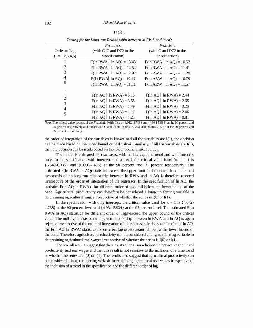
Table 1 reports the F-statistics with different lags in the specification and the critical values at the 90 percent and 95 percent levels. The asymptotic distribution of the F-statistic is non-standard under the null hypothesis that there exists no level relationship irrespective of whether the regressors are I(0) or I(1). Two sets of critical values are provided: one when all regressors are purely I(0) and the other if they are all purely I(1). These two sets of critical values provide a band covering all the possible classifications of the regressors into purely I(0), purely I(1) or mutually cointegrated. If the test statistic exceeds the upper critical value, the null hypothesis of no long-run relationship can be rejected regardless of whether the underlying orders of integration of the variables are zero or one. Similarly, if the test statistic falls below the lower critical value, the null hypothesis is not rejected. If the test statistic falls between the two critical bounds, the result is inconclusive and information on the time series properties of the variables is required. When


Table 1

Testing for the Long-run Relationship between ln RWA and ln AQ

Order of Lag (l = 1,2,3,4,5)

F-statistic (with C, T and D72 in the

Specification)

F-statistic (with C and D72 in the

Specification) 1 2 3 4 5 1 2 3 4 5

F(ln RWA ln AQ) = 18.43 F(ln RWA ln AQ) = 14.54 F(ln RWA ln AQ) = 12.92 F(ln RWA ln AQ) = 10.49 F(ln RWA ln AQ) = 11.11

F(ln AQ ln RWA) = 5.15 F(ln AQ ln RWA) = 3.55 F(ln AQ ln RWA) = 1.49 F(ln AQ ln RWA) = 1.17 F(ln AQ ln RWA) = 1.23

F(ln RWA ln AQ) = 10.52 F(ln RWA ln AQ) = 11.41 F(ln RWA ln AQ) = 11.29 F(ln ARW ln AQ) = 10.79 F(ln ARW ln AQ) = 11.57

F(ln AQ ln RWA) = 2.44 F(ln AQ ln RWA) = 2.65 F(ln AQ ln RWA) = 3.25 F(ln AQ ln RWA) = 2.46 F(ln AQ ln RWA) = 0.81

Note: The critical value bounds of the F-statistic (with C) are {4.042–4.788} and {4.934-5.934} at the 90 percent and 95 percent respectively and those (with C and T) are {5.649–6.335} and {6.606–7.423} at the 90 percent and 95 percent respectively.

the order of integration of the variables is known and all the variables are I(1), the decision can be made based on the upper bound critical values. Similarly, if all the variables are I(0), then the decision can be made based on the lower bound critical values.

The model is estimated for two cases: with an intercept and trend and with intercept only. In the specification with intercept and a trend, the critical value band for k = 1 is {5.649-6.335} and {6.606-7.423} at the 90 percent and 95 percent respectively. The estimated F(ln RWAln AQ) statistics exceed the upper limit of the critical band. The null hypothesis of no long-run relationship between ln RWA and ln AQ is therefore rejected irrespective of the order of integration of the regressor. In the specification of ln AQ, the statistics F(ln AQln RWA) for different order of lags fall below the lower bound of the band. Agricultural productivity can therefore be considered a long-run forcing variable in determining agricultural wages irrespective of whether the series is I(0) or I(1).

In the specification with only intercept, the critical value band for k = 1 is {4.042-4.788} at the 90 percent level and {4.934-5.934} at the 95 percent level. The estimated F(ln RWAln AQ) statistics for different order of lags exceed the upper bound of the critical value. The null hypothesis of no long-run relationship between ln RWA and ln AQ is again rejected irrespective of the order of integration of the regressor. In the specification of ln AQ, the F(ln AQln RWA) statistics for different lag orders again fall below the lower bound of the band. Therefore agricultural productivity can be considered a long-run forcing variable in determining agricultural real wages irrespective of whether the series is I(0) or I(1).

The overall results suggest that there exists a long-run relationship between agricultural productivity and real wages and that this result is not sensitive to the inclusion of a time trend or whether the series are I(0) or I(1). The results also suggest that agricultural productivity can be considered a long-run forcing variable in explaining agricultural real wages irrespective of the inclusion of a trend in the specification and the different order of lag.


Estimating the Coefficients of the Long-run Relationship

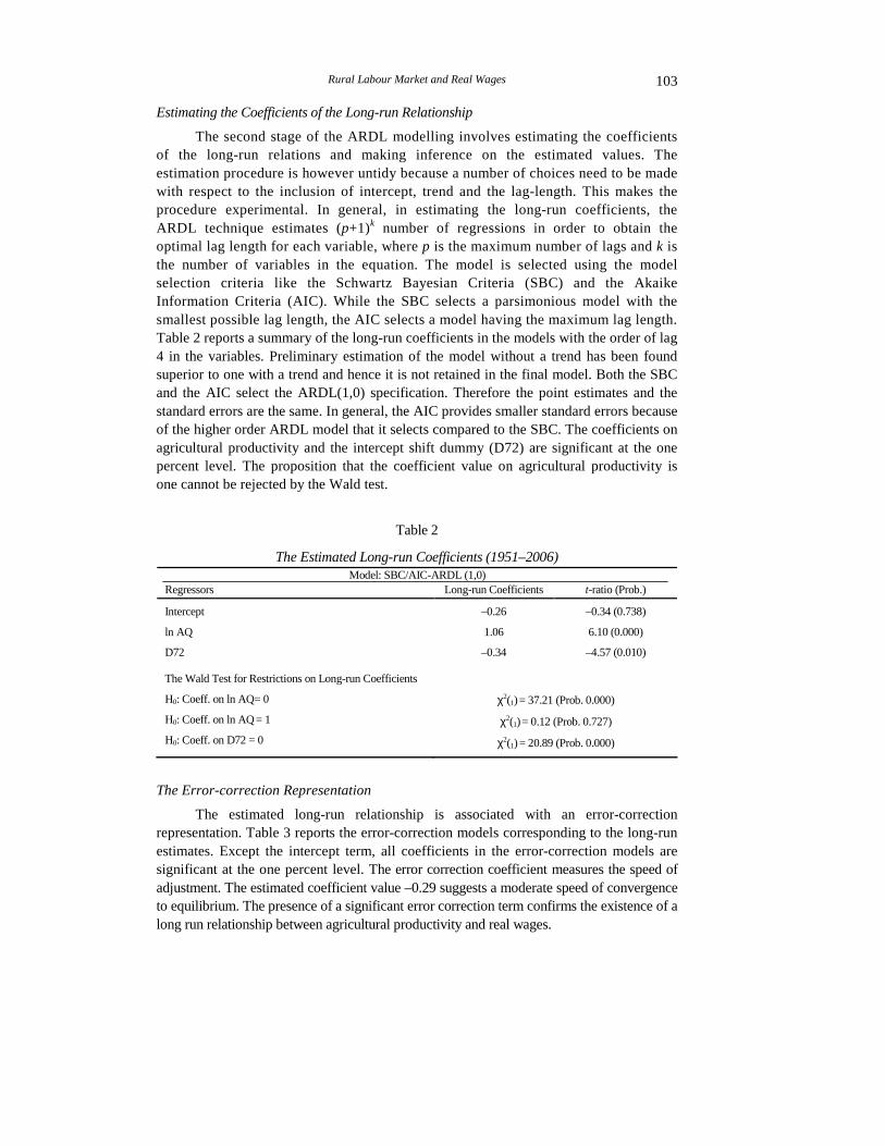
The second stage of the ARDL modelling involves estimating the coefficients of the long-run relations and making inference on the estimated values. The estimation procedure is however untidy because a number of choices need to be made with respect to the inclusion of intercept, trend and the lag-length. This makes the procedure experimental. In general, in estimating the long-run coefficients, the ARDL technique estimates (p+1)k number of regressions in order to obtain the optimal lag length for each variable, where p is the maximum number of lags and k is the number of variables in the equation. The model is selected using the model selection criteria like the Schwartz Bayesian Criteria (SBC) and the Akaike Information Criteria (AIC). While the SBC selects a parsimonious model with the smallest possible lag length, the AIC selects a model having the maximum lag length. Table 2 reports a summary of the long-run coefficients in the models with the order of lag 4 in the variables. Preliminary estimation of the model without a trend has been found superior to one with a trend and hence it is not retained in the final model. Both the SBC and the AIC select the ARDL(1,0) specification. Therefore the point estimates and the standard errors are the same. In general, the AIC provides smaller standard errors because of the higher order ARDL model that it selects compared to the SBC. The coefficients on agricultural productivity and the intercept shift dummy (D72) are significant at the one percent level. The proposition that the coefficient value on agricultural productivity is one cannot be rejected by the Wald test.

Table 2

The Estimated Long-run Coefficients (1951–2006) Model: SBC/AIC-ARDL (1,0)

Regressors Long-run Coefficients t-ratio (Prob.)

Intercept

ln AQ

D72

–0.26

1.06

–0.34

–0.34 (0.738)

6.10 (0.000)

–4.57 (0.010)

The Wald Test for Restrictions on Long-run Coefficients

H0: Coeff. on ln AQ= 0

H0: Coeff. on ln AQ = 1

H0: Coeff. on D72 = 0

χ2(1) = 37.21 (Prob. 0.000)

χ2(1) = 0.12 (Prob. 0.727)

χ2(1) = 20.89 (Prob. 0.000)

The Error-correction Representation

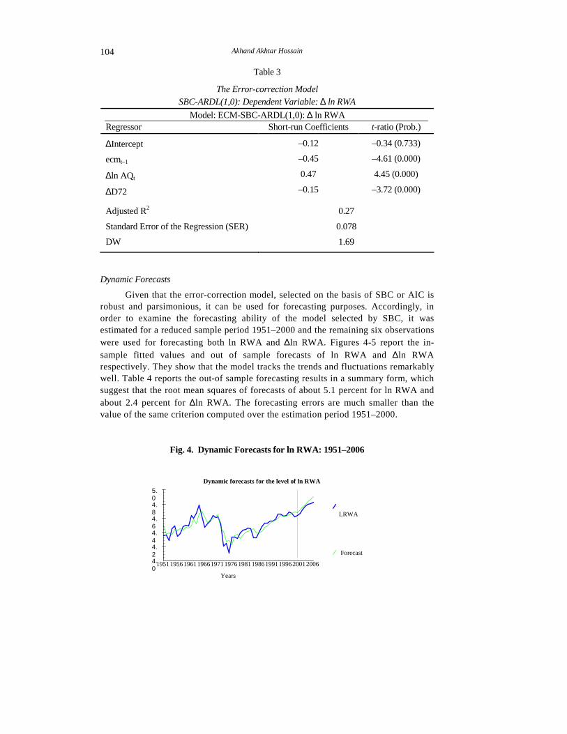
The estimated long-run relationship is associated with an error-correction representation. Table 3 reports the error-correction models corresponding to the long-run estimates. Except the intercept term, all coefficients in the error-correction models are significant at the one percent level. The error correction coefficient measures the speed of adjustment. The estimated coefficient value –0.29 suggests a moderate speed of convergence to equilibrium. The presence of a significant error correction term confirms the existence of a long run relationship between agricultural productivity and real wages.


Table 3

The Error-correction Model SBC-ARDL(1,0): Dependent Variable: ∆ ln RWA

Model: ECM-SBC-ARDL(1,0): ∆ ln RWA

Regressor Short-run Coefficients t-ratio (Prob.)

∆Intercept

ecmt–1

∆ln AQt

∆D72

–0.12

–0.45

0.47

–0.15

–0.34 (0.733)

–4.61 (0.000)

4.45 (0.000)

–3.72 (0.000)

Adjusted R2

Standard Error of the Regression (SER)

DW

0.27

0.078

1.69

Dynamic Forecasts

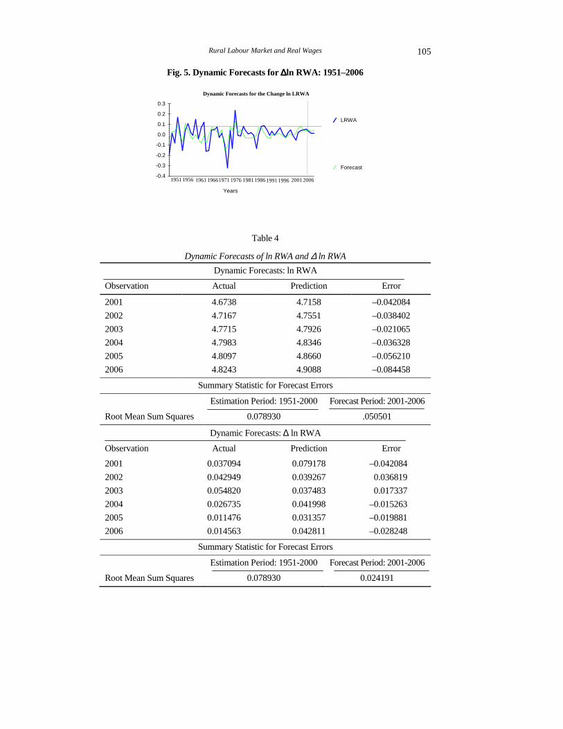
Given that the error-correction model, selected on the basis of SBC or AIC is robust and parsimonious, it can be used for forecasting purposes. Accordingly, in order to examine the forecasting ability of the model selected by SBC, it was estimated for a reduced sample period 1951–2000 and the remaining six observations were used for forecasting both ln RWA and ∆ln RWA. Figures 4-5 report the in-sample fitted values and out of sample forecasts of ln RWA and ∆ln RWA respectively. They show that the model tracks the trends and fluctuations remarkably well. Table 4 reports the out-of sample forecasting results in a summary form, which suggest that the root mean squares of forecasts of about 5.1 percent for ln RWA and about 2.4 percent for ∆ln RWA. The forecasting errors are much smaller than the value of the same criterion computed over the estimation period 1951–2000.

Fig. 4. Dynamic Forecasts for ln RWA: 1951–2006

Dynamic forecasts for the level of ln RWA

LRWA

Forecast

Years 4.0

4.2

4.4

4.6

4.8

5.0

1951 1956 1961 1966 1971 1976 1981 1986 1991 1996 2001 2006


Fig. 5. Dynamic Forecasts for ∆∆∆∆ln RWA: 1951–2006

Table 4

Dynamic Forecasts of ln RWA and ∆ ln RWA

Dynamic Forecasts: ln RWA

Observation Actual Prediction Error

2001

2002

2003

2004

2005

2006

4.6738

4.7167

4.7715

4.7983

4.8097

4.8243

4.7158

4.7551

4.7926

4.8346

4.8660

4.9088

–0.042084

–0.038402

–0.021065

–0.036328

–0.056210

–0.084458

Summary Statistic for Forecast Errors

Estimation Period: 1951-2000 Forecast Period: 2001-2006

Root Mean Sum Squares 0.078930 .050501

Dynamic Forecasts: ∆ ln RWA

Observation Actual Prediction Error

2001

2002

2003

2004

2005

2006

0.037094

0.042949

0.054820

0.026735

0.011476

0.014563

0.079178

0.039267

0.037483

0.041998

0.031357

0.042811

–0.042084

0.036819

0.017337

–0.015263

–0.019881

–0.028248

Summary Statistic for Forecast Errors

Estimation Period: 1951-2000 Forecast Period: 2001-2006

Root Mean Sum Squares 0.078930 0.024191

Dynamic Forecasts for the Change ln LRWA

LRWA

Forecast

Years

-0.1 -0.2 -0.3 -0.4

0.0 0.1 0.2 0.3

1951 1956 1961 1966 1971 1976 1981 1986 1991 1996 2001 2006


VI. SUMMARY AND CONCLUSION

This paper has provided an overview of recent developments in rural labour markets in Bangladesh and also examined the trends and movements of agricultural productivity and real wages with annual data for the period 1950-2006. As part of empirical investigation, the paper has developed a simple model of agricultural real wages that depend on agricultural productivity. In order to examine the long-run relationship between agricultural productivity and real wages, the paper has applied the Autoregressive Distributed Lag bounds testing approach. Empirical results suggest that there exists a long-run relationship between agricultural productivity and real wages and that agricultural productivity can be treated as a ‘long-run forcing variable’ in explaining agricultural real wages. In the short-run dynamic specification of real wages, the coefficient on one-period lagged error-correction term bears the expected negative sign and is highly significant. The forecasting ability of the error correction model is satisfactory with respect to the level or the percentage change of real wages. The overall results are consistent with the findings of earlier studies that agricultural productivity is a key determinant of real wages in Bangladesh.

Empirical results obtained in the paper have some policy implications. Despite Bangladesh being considered a labour surplus country, agricultural real wages have been found to respond to productivity and probably other factors that affect the demand for and supply of labour. An implication is that productivity enhancing technological adoption and other measures, such as opening up the economy that creates external demand for agricultural products, would raise real wages. Given the ongoing integration of the economy, any shift in labour from farm to non-farm activities would also affect agricultural real wages. Although agriculture remains vulnerable to supply shocks that affect the demand for labour, the structural change that has taken place in the economy since the late 1980s appear to have lowered the sensitivity of agricultural real wages to supply shocks because of the increasing non-farm employment opportunities in both the rural and urban areas that has significantly increased the intersectoral labour mobility.

Appendix A

DATA SOURCES AND THE UNIT ROOT TEST RESULTS Real Wages in Agriculture (RWA)

Agricultural nominal wage rate represents the daily wage rate in agriculture in Rupee/Taka per person without food or payments in kind. The annual wage rate is the unweighted average of the average daily wage rates over 12-months. The wage data for the period 1949-69 are for the calendar year and thereafter the wage rates are for the fiscal year that begins in July and ends in June of the following year. The nominal wages for the period 1949-69 are taken from Bose (1974) and thereafter the wages data are taken from various issues of the Statistical Yearbook of Bangladesh and the Yearbook of Agricultural Statistics of Bangladesh. For missing data in 1954, interpolation is made. Data for the cost of living for rural households for the period 1949-69 and 1970-1978 are taken from Bose (1974) and Khan (1984) respectively. The remaining data are taken from


various issues of the Statistical Yearbook of Bangladesh, the Yearbook of Agricultural Statistics of Bangladesh, the Bangladesh Economic Review and the Economic Trends. The Bangladesh Bureau of Statistics, the Ministry of Finance of the Government of Bangladesh and the Bangladesh Bank publish these statistical publications. The real wage rate is calculated as the nominal wage rate index deflated by the cost of living index for rural households with a common base (1969 = 100). Agricultural Output per Gross Cropped Acreage (AQ)

Data for the index of agricultural output per-gross cropped acreage for the period 1950-1981 are taken from Boyce and Ravallion (1987) and thereafter the data are generated from output and acreage statistics published in various issues of the Statistical Yearbook of Bangladesh. The data series have been transformed into a common base 1950=100.

Tables A1-A2 report the two widely used unit root test results. They are the augmented Dickey-Fuller (ADF) and the Kwiatkowski, Phillips, Schmidt and Shin (KPSS) tests. The first test treats the series under consideration non-stationary as a null hypothesis while the second test treats the series under consideration stationary as a null hypothesis. It is better when these tests results are consistent or confirmatory because most unit root tests have low power, especially when the sample size is small [Maddala (2001)]. For testing purposes, both the series have been transformed into natural logarithmic forms. The tests have been conducted for the sample period 1950–2006. The adjusted sample size is however smaller depending on the number of lag terms used in the specification. As the tests results are sensitive to lag length, the test statistics have been generated for up to 5 lags of the first-difference of the variable in the logarithmic form and then the Schwartz Bayesian Criterion has been used to select the optimal lag length under the restriction that the maximum lag length is 5. Because the data are annual, five lag terms have been found more than adequate to make the residuals in the regression a white noise. Both the ADF and the KPSS tests results suggest that agricultural real wages and agricultural productivity have a unit root. Although this finding may be considered adequate, to confirm this finding the Perron test is conducted where allowance is made for any structural break in the data series in 1972. The Perron Test for Unit Root with a Structural Break in 1972

Perron (1989, 1990) has demonstrated that the standard Dickey-Fuller tests for unit roots could be biased toward accepting the null hypothesis of a unit root against trend-stationary alternatives if the true data generating mechanism is that of stationary around a trend with a one-time structural break. This implies that if an allowance is made for the once and for all change in the level and/or in the slope of the trend function because of a structural break, the time series of a macroeconomic variable may reject the null hypothesis of a unit root. Perron (1989) has devised tests that can be conducted for unit roots in the time series of variables by making allowance of a structural break in the series. The essence of his methodology is to detrend the original series with an allowance for a structural break and to conduct tests for unit roots in the detrended series. As a follow up of Perron’s (1989) methodology, Perron (1997), Perron and Vogelsang (1992) and Zviot and Andrews (1992) have developed testing procedures that can be used to determine the structural break as an unknown parameter. In this paper, Perron’s (1989)

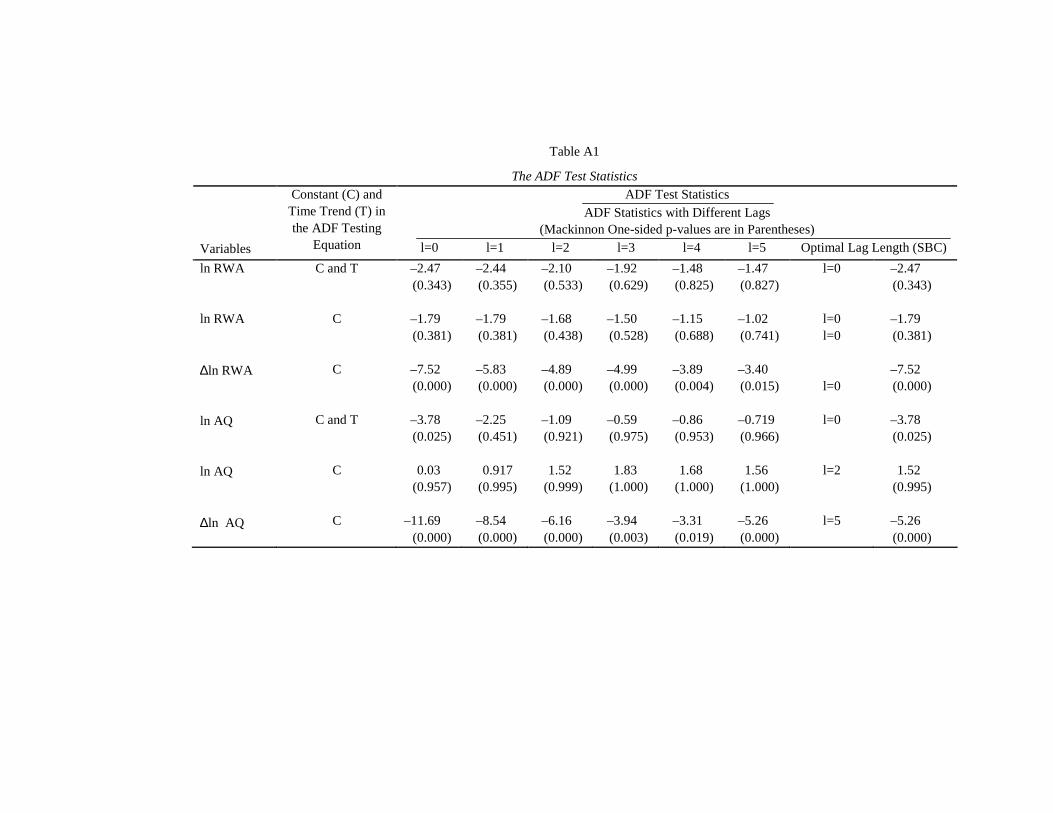
Table A1

The ADF Test Statistics ADF Test Statistics

ADF Statistics with Different Lags (Mackinnon One-sided p-values are in Parentheses)

Variables

Constant (C) and Time Trend (T) in the ADF Testing

Equation l=0 l=1 l=2 l=3 l=4 l=5 Optimal Lag Length (SBC)

ln RWA

ln RWA ∆ln RWA

ln AQ

ln AQ ∆ln AQ

C and T

C

C

C and T

C

C

–2.47 (0.343)

–1.79 (0.381)

–7.52 (0.000)

–3.78 (0.025)

0.03

(0.957)

–11.69 (0.000)

–2.44 (0.355)

–1.79 (0.381)

–5.83 (0.000)

–2.25 (0.451)

0.917

(0.995)

–8.54 (0.000)

–2.10 (0.533)

–1.68 (0.438)

–4.89 (0.000)

–1.09 (0.921)

1.52

(0.999)

–6.16 (0.000)

–1.92 (0.629)

–1.50 (0.528)

–4.99 (0.000)

–0.59 (0.975)

1.83

(1.000)

–3.94 (0.003)

–1.48 (0.825)

–1.15 (0.688)

–3.89 (0.004)

–0.86 (0.953)

1.68

(1.000)

–3.31 (0.019)

–1.47 (0.827)

–1.02 (0.741)

–3.40 (0.015)

–0.719 (0.966)

1.56

(1.000)

–5.26 (0.000)

l=0

l=0 l=0

l=0

l=0

l=2

l=5

–2.47 (0.343)

–1.79 (0.381)

–7.52 (0.000)

–3.78 (0.025)

1.52

(0.995)

–5.26 (0.000)

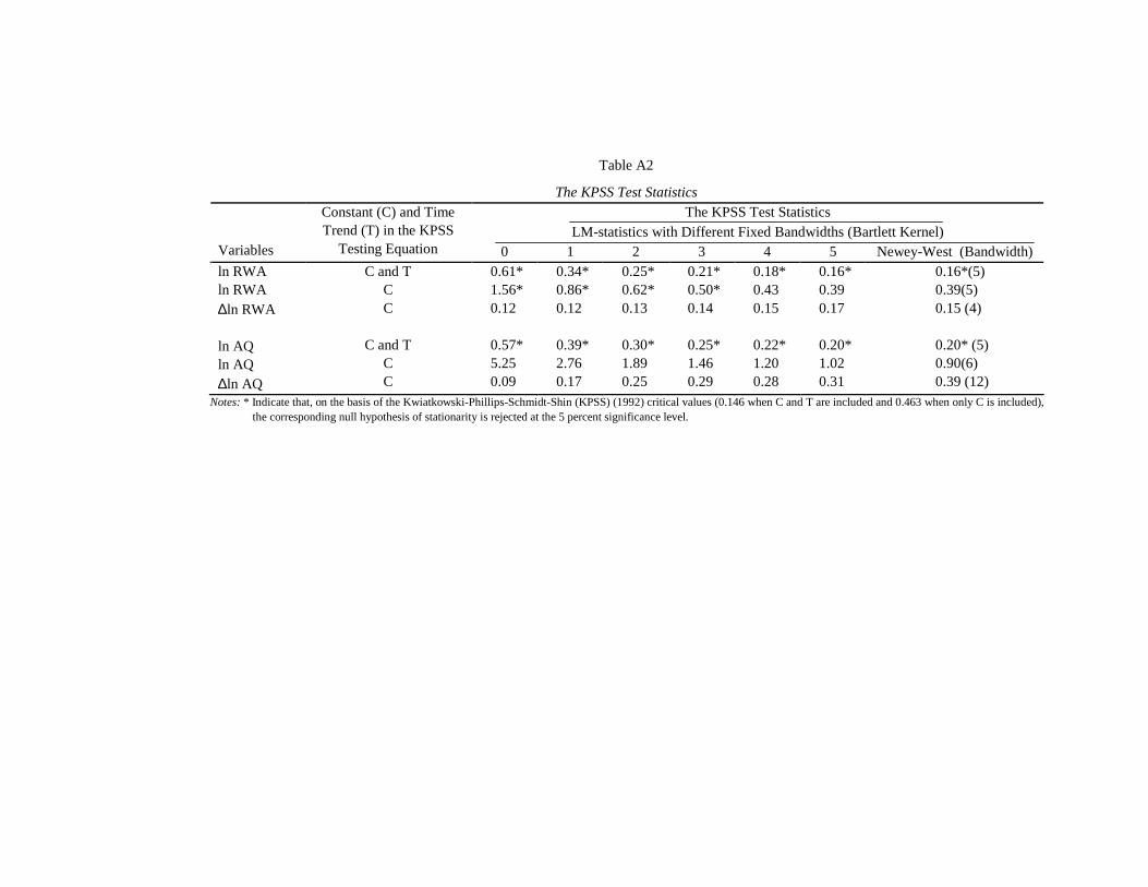
Table A2

The KPSS Test Statistics The KPSS Test Statistics

LM-statistics with Different Fixed Bandwidths (Bartlett Kernel) Variables

Constant (C) and Time Trend (T) in the KPSS

Testing Equation 0 1 2 3 4 5 Newey-West (Bandwidth) ln RWA ln RWA ∆ln RWA

ln AQ ln AQ

∆ln AQ

C and T C C

C and T C C

0.61* 1.56* 0.12

0.57* 5.25 0.09

0.34* 0.86* 0.12

0.39* 2.76 0.17

0.25* 0.62* 0.13

0.30* 1.89 0.25

0.21* 0.50* 0.14

0.25* 1.46 0.29

0.18* 0.43 0.15

0.22* 1.20 0.28

0.16* 0.39 0.17

0.20* 1.02 0.31

0.16*(5) 0.39(5) 0.15 (4)

0.20* (5) 0.90(6) 0.39 (12)

Notes: * Indicate that, on the basis of the Kwiatkowski-Phillips-Schmidt-Shin (KPSS) (1992) critical values (0.146 when C and T are included and 0.463 when only C is included), the corresponding null hypothesis of stationarity is rejected at the 5 percent significance level.


test is chosen because Bangladesh’s independence in 1971 can be considered a well-defined exogenous event. Assuming that this might have caused a structural break in the data series, the Perron test is conducted to confirm the results reported above.

The two-step procedure of the Perron test is as follows:

xt = µ1 + β1 t + (µ1–µ2) D72t + (β1–β2) DT72t + z t … … … (1)

zt = ρ zt–1 + Σγi∆zt–i + ut (i = 1,2,3,…) … … … … (2)

where xt is the generic variable whose time series is subjected to unit root testing, t is a linear time trend (t =1,2,…T), D72 = 1 if t>TB (TB refers to the structural break or event at which changes have occurred in the parameters of the trend function) and zero otherwise, DT 72 = t if t>TB and zero otherwise, z is the residual or detrended structural-break adjusted value for xt and u is a random error term.

Equation (2) is estimated in the following form:

∆zt = (ρ–1) zt–1+ Σγi∆zt–i + u t (i = 0,1,2,3,4,5) … … … … (3)

The test for the random walk hypothesis is a test for the zero restriction on

θ (=ρ–1). It shows that the Perron test is essentially the Dickey-Fuller test on the detrended series zt. The critical values for the Perron test are however different from those required for the Dickey-Fuller test. In the Perron test, the critical values depend on

λ, which is calculated as the observation number at which the break is suspected to have

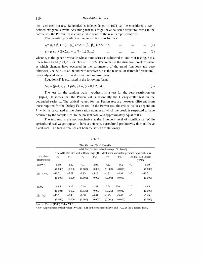
occurred by the sample size. In the present case, λ is approximately equal to 0.4. The test results are not conclusive at the 5 percent level of significance. While

agricultural real wages appear to have a unit root, agricultural productivity does not have a unit root. The first differences of both the series are stationary.

Table A3

The Perron Test Results ADF Test Statistics (No Intercept, No Trend)

The ADF statistics with different lags (The Mackinnon one-sided p-values in parentheses) Variables

(Detrended) l=0 l=1 l=2 l=3 l=4 l=5 Optimal Lag Length

(SBC)

ln RWA

∆ln RWA

ln AQ

∆ln AQ

–5.99

(0.000)

–10.31

(0.000)

–4.85

(0.001)

–11.91

(0.000)

–4.82

(0.000)

–7.09

(0.000)

–3.17

(0.002)

–8.48

(0.000)

–4.71

(0.000)

–6.93

(0.000)

–2.18

(0.030)

–6.30

(0.000)

–3.96

(0.000)

–5.13

(0.000)

–1.81

(0.067)

–4.01

(0.000)

–4.13

(0.000)

–4.21

(0.000)

–2.24

(0.025)

–3.45

(0.001)

–4.66

(0.000)

–4.99

(0.000)

–230

(0.022)

–5.45

(0.000)

l=0

l=0

l=0

l=5

–5.99

(0.000)

–10.31

(0.000)

–4.85

(0.000)

–5.45

(0.000)

Source: Perron (1989): Table VI.B. Note: Approximate critical values (λ≈0.4): –4.81 at the one percent level and –4.22 at the 5 percent level.


REFERENCES

Abdullah, A. A., and Q. Shahabuddin (1997) Critical Issues in Agriculture: Policy Response and Unfinished Agenda. In M.G. Quibria (ed.) The Bangladesh Economy in Transition. Dhaka: University Press Limited.

Ahmed, I. (1981) Wage Determination in Bangladesh Agriculture. Oxford Economic Papers 33, 298–322.

Ahmed, S. and Z. Sattar (2004) Trade Liberalisation, Growth and Poverty Reduction: The Case of Bangladesh. South Asia Region of the World Bank, Washington, DC. (Processed.)

Alam, G. M. M., M. S. Rahman, and M. A. S. Mandal (2004) Backward and Forward Linkages of Power Tiller Technology: Some Empirical Insights from an Area of Bangladesh. Bangladesh Journal of Political Economy 20:1, 139–152.

Alamgir, M., and L. J. J. B. Berlage (1974) Bangladesh: National Income and Expenditure 1949-50–1969-70. Bangladesh Institute of Development Studies, Dhaka. (Research Monograph No.1.)

Amin, A. T. M. N. (1981) Marginalisation vs. Dynamism: A Study of the Informal Sector in Dacca City. Bangladesh Development Studies 9:4, 77–112.

Asian Development Bank (ADB) (2005) Labour Markets in Asia: Promoting Full, Productive, and Decent Employment. Special Chapter of Key Indicators of Developing Asian and Pacific Countries. Manila: Asian Development Bank.

Bangladesh Bank (Various Issues) Economic Trends. Dhaka: Bangladesh Bank. Bangladesh Bureau of Statistics (2003) Twenty Years of National Accounting. Dhaka:

Bangladesh Bureau of Statistics. Bangladesh Bureau of Statistics (Various Issues) Economic Indicators of Bangladesh.

Dhaka: Bangladesh Bureau of Statistics. Bangladesh Bureau of Statistics (Various Years) Statistical Yearbook of Bangladesh. Dhaka:

Bangladesh Bureau of Statistics. Bangladesh Bureau of Statistics (Various Years) The Agricultural Statistical Yearbook of

Bangladesh. Dhaka: Bangladesh Bureau of Statistics. Bangladesh, Government of (Various Issues) Bangladesh Economic Review. Dhaka:

Ministry of Finance. Bardhan, K. (1973) Factors Affecting Wage Rates for Agricultural Labour. Economic and

Political Weekly 8, A56–A63. Bardhan, K. (1977) Rural Employment, Wages and Labour Markets in India: A Survey of

Research, Part I, Part II, and Part III. Economic and Political Weekly 12, A34–A48; 1062–1074; 1108–1118.

Bardhan, P. (1973) Size, Productivity and Returns to Scale: An Analysis of Farm Level Data in Indian Agriculture. Journal of Political Economy 81, 1370–1386.

Bardhan, P. (1977) Determinants of Supply and Demand for Labour in a Poor Agrarian Economy: An Analysis of Household Data in Rural West Bengal. (Mimeographed.)

Bardhan, P. (1979a) Labour Supply Functions in a Poor Agrarian Economy. American Economic Review 69, 73–83.

Bardhan, P. (1979b) Wages and Unemployment in a Poor Agrarian Economy: A Theoretical and Empirical Analysis. Journal of Political Economy 87, 479–500.


Bose, S. R. (1974) Movement of Agricultural Wages in Bangladesh 1949-73. In A. Mitra (ed.) Economic Theory and Planning. Calcutta: Oxford University Press.

Boyce, J., and M. Ravallion (1987) Intersectoral Terms of Trade and the Dynamics of Wage Determination in Bangladesh. Canberra; Australian National University. (Unpublished Manuscript.)

Boyce, J., and M. Ravallion (1991) A Dynamic Econometric Model of Agricultural Wage Determination in Bangladesh. Oxford Bulletin of Economics and Statistics 53:4, 361–376.

Engle, R., and C. Granger (1987) Cointegration and Error Correction: Representation, Estimation and Testing. Econometrica 55, 251–276.

Hansen, B. (1966) Marginal Productivity Wage Theory and Subsistence Wage Theory in Egyptian Agriculture. Journal of Development Studies 2, 367–407.

Hansen, B. (1969) Employment and Wages in Rural Egypt. American Economic Review 59, 298–313.

Hansen, B. (1971) Employment and Rural Wages in Egypt: Reply. American Economic Review 61, 500–508.

Hanson, J. (1971) Employment and Rural Wages in Egypt: A Reinterpretation. American Economic Review 61, 492–499.

Hossain, A. (1990) Real Wage Determination in Bangladesh Agriculture. Applied Economics 22, 1549–1565.

Hossain, A. (1995) Inflation, Economic Growth and the Balance of Payments in Bangladesh: A Macroeconomic Study. Delhi: Oxford University Press.

Hossain, A. (1996) Macroeconomic Issues and Policies: The Case of Bangladesh. New Delhi: Sage Publications.

Hossain, A. (2000) Exchange Rates, Capital Flows and International Trade: The Case of Bangladesh. Dhaka: The University Press Limited.

Hossain, A. (2006) Overview of the Bangladesh Economy, In A. Hossain, F. Khan and T. Akram (eds.) Economic Analyses of Contemporary Issues in Bangladesh. Dhaka: The University Press.

Hossain, A. (2007) Labour Market Developments in Bangladesh since the Mid-1980s. In J. Burgess and J. Connell (eds.) Globalisation and Work in Asia. 93–127. Oxford: Chandos Publishing.

Hossain, M. (1988) Nature and Impact of the Green Revolution in Bangladesh. Washington, DC: International Food Policy Research Institute. (Research Paper 67.)

Hossain, M., M. L. Bose, A. Chowdhury, and R. Meimzen-Dick (2002) Changes in Agrarian Relations and Livelihoods in Rural Bangladesh: Insights from Repeat Village Studies. In V.K. Ramachandran and M. Swaminathan (eds.) Agrarian Studies: Essays on Agrarian Relations in Less Developed Countries. Proceedings of the International Conference on Agrarian Relations and Rural Development in Less Developed Countries, New Delhi.

Johansen, S. (1988) Statistical Analysis of Cointegration Vectors. Journal of Economic Dynamics and Control 12, 231–254.

Johansen, S., and K. Juselius (1990) Maximum Likelihood Estimation and Inference on Cointegration with Applications to the Demand for Money. Oxford Bulletin of Economics and Statistics 52, 169–210.


Khan, A. R. (1984) Real Wages of Agricultural Workers in Bangladesh. In A. R. Khan and E. Lee (eds.) Poverty in Rural Asia. Bangkok: ILO-ARTEP.

Kwiatkowski, D., P. C. B. Phillips, P. Schmidt, and Y. Shin (1992) Testing the Null Hypothesis of Stationarity Against the Alternative of a Unit Root: How Sure are We that Economic Time Series Have a Unit Root? Journal of Econometrics 54, 159–178.

Lewis, P. and G. Makepeace (1984) The Estimation of a Disequilibrium Real Wage Equation for Britain. Journal of Macroeconomics 6, 399–410.

Lewis, P. and M. Kirby (1987) The Impact of Incomes Policy on Aggregate Wage Determination in Australia. Economic Record 63, 156–161.

Lewis, W. A. (1954) Economic Development with Unlimited Supplies of Labour. Manchester School 22, 139–191.

Maddala, G. S. (2001) Introduction to Econometrics, (3rd Edition). New York: John Wiley and Sons.

McFadden, D. (1978) Cost, Revenue, and Profit Functions. In M. Fuss and D. McFadden (eds.) Production Economics: A Dual Approach to Theory and Applications 1, 3–109. Amsterdam: North-Holland Publishing Company.

Palmer-Jones, R. W. (1993) Agricultural Wages in Bangladesh: What the Figures Really Show? Journal of Development Studies 29, 277–300.

Palmer-Jones, R. W. (1994) An Error-Corrected? And What the Figures Really Show? Journal of Development Studies 31:2, 346–351.

Perron, P. (1989) The Great Crash, the Oil Price Shock, and the Unit Root Hypothesis. Econometrica 57:6, 1361–1401.

Perron, P. (1990) Testing for a Unit Root in a Time Series with a Changing Mean. Journal of Business and Economic Statistics 8, 153–162.

Perron, P. (1997) Further Evidence on Breaking Trend Functions in Macroeconomic Variables. Journal of Econometrics 80:2, 355–85.

Perron, P., and T. J. Vogelsang (1992) Nonstationarity and Level Shifts with an Application to Purchasing Power Parity. Journal of Business and Economic Statistics 10, 301–320.

Pesaran, M. H. and R. Smith (1998) Structural Analysis of Cointegration VARs. Journal of Economic Surveys 12, 471–505.

Pesaran, M. H., and B. Pesaran (1997) Working with Microfit 4.0: Interactive Econometric Analysis. Oxford: Oxford University Press.

Pesaran, M. H., and Y. Shin (1996) Cointegration and Speed of Convergence to Equilibrium. Journal of Econometrics 71, 117–43.

Pesaran, M. H., Y. Shin, and R. Smith (2001) Bounds Testing Approaches to the Analysis of Level Relationships. Journal of Applied Econometrics 16:3, 289–326.

Rashid, S. (2002) Dynamics of Agricultural Wage and Rice Price in Bangladesh: A Re-Examination. Washington, DC: International Food Policy Research Institute. (Markets and Structural Studies Division Discussion Paper No. 44.)

Ravallion, M. (1994) Agricultural Wages in Bangladesh: What Do the Figures Really Show? Journal of Development Studies 31:2, 334–345.

Rosen, H., and R. Quandt (1978) Estimation of a Disequilibrium Aggregate Labour Market. Review of Economics and Statistics 60, 371–379.


Rosenzweig, M. (1978) Rural Wages, Labor Supply and Land Reform: A Theoretical and Empirical Analysis. American Economic Review 68, 847–861.

Rosenzweig, M. (1980) Neoclassical Theory and the Optimising Peasant: An Econometric Analysis of Market Family Labour Supply in a Developing Country. Quarterly Journal of Economics 94, 31–55.

Schumpeter, J. (1981) History of Economic Analysis. Sydney: George Allen and Unwin. Sen, A. K. (1960) Choice of Techniques. Oxford: Basil Blackwell. Shahabuddin, Q. (1985) Testing of Cobb-Douglas Myths: An Analysis with

Disaggregated Production Functions in Bangladesh Agriculture. Bangladesh Development Studies 13, 87–98.

Spiegel, H. (1971) The Growth of Economic Thought. New Jersey: Prentice-Hall. Squire, L. (1981) Employment Policy in Developing Countries: A Survey of Issues and

Evidence. World Bank Research Publication. New York: Oxford University Press. Sraffa, P. (ed.) (1970) The Works and Correspondence of David Ricardo. Cambridge:

Cambridge University Press. Todaro, M. P., and S. C. Smith (2003) Economic Development. New York: Addison-Wesley. Varian, H. (1984) Microeconomic Analysis. New York: Norton and Company. World Bank (2003) Bangladesh: Development Policy Review. Poverty Reduction and

Economic Management Sector Unit, South Asia Region, World Bank. (Report No.26154-BD.)

Zivot, E., and D. W. K. Andrews (1992) Further Evidence on the Great Crash, the Oil Price Shock, and the Unit Root Hypothesis. Journal of Business and Economic Statistics 10:3, 251–270.

Documents

Rural Labour Market Developments, Agricultural ... Labour Market Developments, Agricultural Productivity, and Real Wages in Bangladesh, 1950–2006 ... The focus of this paper is developments