Rules of Origin as Export Subsidies ¤

Olivier Cadot y

Antoni Estevadeordal z

Akiko Suwa-Eisenmann x

February 2004

AbstractThe paper estimates the e¤ect of NAFTA’s rules of origin (ROO)

on Mexican access to the US market treating explicitly the endoge-nous determination of ROOs. The …rst equation determines Mexico’sNAFTA (preferential) exports to the US as a function of tari¤ prefer-ence and Estevadeordal’s qualitative ROO index. The second equationdetermines ROOstrictness on the basis of a Grossman-Helpman modelidentifying channels through which lobbying by US intermediate-goodproducers leads to deep preferences and sti¤ rules of origin in down-stream sectors. The estimates suggest that the creation of a captivemarket for upstream intermediate-good producers is indeed one oftheir political determinants.

JEL classi…cation numbers: F10, F13, F15¤This research was produced as part of an IADB research program. We are thankful to

Celine Carrere, Jon Haveman, Jim de Melo, Marcelo Olarreaga, Pablo Sanguinetti, Mau-rice Schi¤, and participants at the IIIrd Workshop of the Regional Integration Network,Punta Del Este, December 2003 and the joint IADB/CEPR workshop, Paris, April 2003for useful comments and suggestions. All errors remain ours, and the views expressed inthis paper do not necessarily re‡ect those of the institutions to which authors are a¢liated.Special thanks to Kati Suominen and to David Colin for superb research assistance.

yHEC Lausanne, CERDI and CEPR.zIADBxDELTA and INRA

Keywords: NAFTA, Rules of Origin, Regional Integration.

2

1 IntroductionWith the proliferation of preferential trading agreements over the last twodecades, considerable attention has been devoted to assessing their e¤ect onmarket access. Notwithstanding the fact that GATT Article XXIV, para.8(b) requires the removal of trade barriers on “substantially all trade” inFree-Trade Agreements (FTAs), in reality numerous barriers to intra-bloctrade are often left intact or even erected as part of the agreements.1 Rulesof Origin (ROOs) feature prominently among those barriers.

In principle, ROOs are meant to prevent the trans-shipment of goodsimported from the rest of the world, via member states with low externaltari¤s, into those with higher ones. In practice, these rules often have thee¤ect of “exporting protection” from high-tari¤ members to low-tari¤ ones,as pointed out by Krishna and Krueger (1995) and Krueger (1997).

In North-South FTAs, in particular, the combination of tari¤ preferencesand ROOs can a¤ect trade ‡ows in ways that are not conducive to economice¢ciency. Suppose that the production of …nal goods involves two stages: thecapital-intensive production of components, and labor-intensive assembly. Ifgoods are entirely produced in the North early on in their product cycle, pref-erential tari¤ reductions may accelerate the process of assembly relocation inthe South, leading to what Hanson (1996) called “regional production net-works”.2 Suppose, however, that component manufacturing could pro…tablybe relocated to another Northern country outside of the preferential tradingbloc. Rules of origin, by forcing Southern assemblers to source a minimumfraction of their components in the area, prevent the ultimate relocation ofthe whole value chain in the world’s most e¢cient location. In other words,ROOs, when they bind, organize trade diversion by creating captive marketsfor relatively ine¢cient Northern intermediate-good producers.

While the potentially trade-diverting e¤ect of ROOs has been widelyrecognized in the literature (see for instance Falvey and Reed, 2000), the re-cent political-economy literature has also highlighted the fact that ROOs cansometimes make preferential agreements politically feasible in circumstanceswhere they wouldn’t be otherwise (Duttagupta, 2000; Duttagupta and Pana-garyia, 2002). As Grossman and Helpman (1995) showed that trade-diverting

1See Serra et al. (1996) for a review of shortcomings in the application of Article XXIV.2However, Hanson also shows that the emergence of vertical trade between Mexico and

the United States largely predates the formation of NAFTA, as assembly plants alreadyaccounted for 53% of Mexico’s manufactured exports in 1992.

FTAs are, ceteris paribus, more likely than others to be politically acceptable,Duttagupta and Panagariya’s result is quite consistent with ROOs acting as“trade diverters”.

While the theoretical analysis of ROOs has made considerable stridessince Krueger’s pioneering work, their empirical analysis is still in its infancy,partly because their complex legal nature makes measurement di¢cult. Es-tevadeordal (2000) recently proposed a way to overcome this di¢culty bydevising a qualitative index of ROO strictness. Using the fact that mostROOs are —at least in recent agreements— expressed as a required changein tari¤ heading at various levels of aggregation, Estevadeordal’s index takesvalues that increase in the level of aggregation of the required change, theidea being that a change at a more aggregate level is “wider” and hence amore stringent transformation requirement. On the basis of his index, heidenti…ed a strong negative e¤ect of NAFTA’s ROOs on Mexican marketaccess. Using the same index, Anson et al. (2003) showed that the e¤ect ofNAFTA’s tari¤ preferences is systematically reduced by ROOs.

Although Anson et al’s results are qualitatively unambiguous, they su¤erfrom the fact that the potential endogeneity of ROOs is not treated. If thereis little doubt that, as pointed out by Estevadeordal (2000) and Sanguinetti(2003), ROOs are the result of a political bargaining process that is itselflikely to be a¤ected by trade patterns, it is not entirely clear, short of afull political-economy model, what exactly they are endogenous to. If theyare endogenous to Mexican …nal-good exports, clearly there is a simultaneityproblem. If, however, ROOs are endogenous to trade ‡ows that are relatedto Mexican exports only through an indirect, nonlinear relationship, for es-timation purposes the relevant system may be recursive rather than trulysimultaneous.

In this paper, we take the endogeneity problem as a starting point for anexploration of the political-economy forces that are likely to shape ROOs.Although many assumptions must be made along the way, we show that ina model of endogenous ROO determination à la Grossman-Helpman (1994),the key determinant of ROOs in terms of trade ‡ows is a product of USintermediate-good exports to Mexico and input-output coe¢cients. Themodel generates results both in terms of interpretation of what ROOs doand in terms of what the estimation strategy should be.

As for interpretative results, the key one is that whereas ROOs create cap-tive markets for US intermediate goods, tari¤ preferences needed to makethem acceptable to Mexican exporters along their participation constraint

2

constitute a transfer —albeit a modest one— from US taxpayers.3 The com-bination of ROOs and tari¤ preference is then equivalent to an export subsidyon US intermediate goods. The model thus proposes a tentative answer, inthis particular context, to a question arising frequently in trade policy—namely, why ine¢cient indirect instruments are used to redistribute incomewhen more direct instruments would achieve the same results at lesser wel-fare costs. Here, ROOs substitute for a prohibited instrument, as exportsubsidies would be in violation of the US’s obligations under the GATT.

Our analysis of rules of origin requires a model with multiple stages ofproduction. In contrast to Lloyd (1993), Rodriguez (2001) and Carrère andde Melo (2004) who use a multi-stage production model due to Dixit andGrossman (1982), our analysis requires only a two-stage Leontie¤ productiontechnology whose analytics are very simple.

As for the estimation, the model suggests, as the key determinant ofNAFTA’s ROOs, a vector product of input-output coe¢cients multiplied byUS intermediate-good exports upstream of the good to which ROOs apply.Our estimation strategy thus consists of regressing ROOs on steady-statetari¤ preferences (equal, at the end of the phase-out period, to the US MFNtari¤ adjusted for exceptions) and the upstream variable just described, thefunctional form being the political-economy model’s …rst-order condition.This generates a vector of predicted ROOs which are then used in the market-access equation. As for tari¤ preferences, we do not model their endogeneitydirectly as intra-NAFTA tari¤s smoothly converge to zero over a …xed phase-out period. A fuller model would recognize, as Estevadeordal (2000) did, thatthe length of the phase-out may itself be endogenous, but the model we usedoes not lend itself easily to taking this into account.

We chose NAFTA as a testing ground because it provides a laboratoryexperiment to test the e¤ect of ROOs. It is the quintessential example of theNorth-South agreement due to the comprehensive tari¤ liberalization built inthe agreement and the fact that member countries share borders, eliminatingthe need to account for distance as in traditional gravity exercises. We con-struct a panel dataset with information dating back to 1989 on commodityexports from Mexico to the United States under di¤erent preferential pro-grams. The data was compiled mostly from USITC sources at the 6-digit HS

3By participation constraint, we mean that the rate of e¤ective protection granted toMexican …nal-good producers by the combination of tari¤ preferences and rules of originis just zero.

3

disaggregation level and contains information on tari¤ preferences (GSP andNAFTA rates) granted by the United States to Mexico. From 1989 to 1994,Mexico’s exports to the United Stated bene…ted from the Generalized Systemof Preferences (GSP), after which this regime was overhauled by NAFTA.The data on rules of origin comes from Estevadeordal (2000).

The results are in conformity with the model’s predictions. All variablesare signi…cant —most of them at the 1% level— and have the expected signs.Tari¤ preferences and ROOs exert positive and negative in‡uences respec-tively on Mexican exports, and the key variable in‡uencing endogenously-determined ROOs —a product of input-output coe¢cients and US interme-diate exports to Mexico— has the predicted sign and is signi…cant at the 1%level.

The paper is organized as follows. Section 2 sets out the political-economymodel and characterizes its equilibrium. Section 3 presents the empiricalmethodology and results, and section 4 concludes.

2 Politically-determined ROOsThis section uses a simple, stripped-down political-economy model to illus-trate the simultaneous determination of tari¤ preferences and ROOs. Al-though the model borrows from Grossman and Helpman (1994) the ap-pearance of a general-equilibrium model, it is best thought of as a partial-equilibrium one as interindustry linkages are nonexistent except for the ver-tical linkages around which the discussion is centered.

2.1 The economyConsider a PTA formed by two small economies, North (N) and South (S).The North produces, under increasing cost, an intermediate good denotedby the subscript I and exports it to the South which uses it to assemble a…nal good denoted by the subscript F . Southern supply of the …nal good isnot enough to cover the North’s consumption at its tari¤-ridden price, so theNorth also imports from the rest of the world. The South imports all its ownconsumption of the …nal good from the rest of the world and exports all itsproduction to the North.4

4This is shown to arise endogenously in Cadot, de Melo and Olarreaga (2001).

4

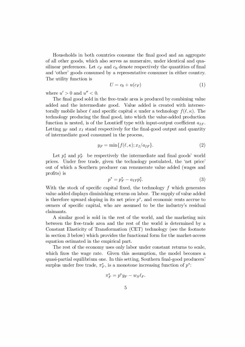
Households in both countries consume the …nal good and an aggregateof all other goods, which also serves as numeraire, under identical and qua-silinear preferences. Let cF and c0 denote respectively the quantities of …naland ‘other’ goods consumed by a representative consumer in either country.The utility function is

U = c0 + u(cF) (1)

where u0 > 0 and u00 < 0.The …nal good sold in the free-trade area is produced by combining value

added and the intermediate good. Value added is created with intersec-torally mobile labor ` and speci…c capital · under a technology f(`; ·). Thetechnology producing the …nal good, into which the value-added productionfunction is nested, is of the Leontie¤ type with input-output coe¢cient aIF .Letting yF and xI stand respectively for the …nal-good output and quantityof intermediate good consumed in the process,

yF = minff(`; ·);xI=aIFg: (2)

Let p¤I and p¤F be respectively the intermediate and …nal goods’ worldprices. Under free trade, given the technology postulated, the ‘net price’out of which a Southern producer can remunerate value added (wages andpro…ts) is

p¤ = p¤F ¡ aIFp¤I: (3)

With the stock of speci…c capital …xed, the technology f which generatesvalue added displays diminishing returns on labor. The supply of value addedis therefore upward sloping in its net price p¤, and economic rents accrue toowners of speci…c capital, who are assumed to be the industry’s residualclaimants.

A similar good is sold in the rest of the world, and the marketing mixbetween the free-trade area and the rest of the world is determined by aConstant Elasticity of Transformation (CET) technology (see the footnotein section 3 below) which provides the functional form for the market-accessequation estimated in the empirical part.

The rest of the economy uses only labor under constant returns to scale,which …xes the wage rate. Given this assumption, the model becomes aquasi-partial equilibrium one. In this setting, Southern …nal-good producers’surplus under free trade, ¼¤F , is a monotone increasing function of p¤:

¼¤F = p¤yF ¡ wS`F :

5

Letting p be the domestic net price, (p¡ p¤)=p is the e¤ective rate of protec-tion granted to Southern producers when selling on the Northern market.5

The intermediate good is produced in the North with value-added onlyunder a technology similar to f (i.e. a CRS combination of labor and speci…ccapital). Letting yI be its output, producer surplus is

¼I = pIyI ¡ wN`I : (4)

Finally, we will measure the intermediate good in units that make its worldprice p¤I equal to one, and we will treat its supply elasticity in the North,"I ´ pIy0I=yI , as a constant.

2.2 The preferential regimeIn order to keep things simple, we will treat MFN (external) tari¤s on the …naland intermediate goods as predetermined to the PTA and hence parametric.Northern tari¤s are respectively tNF and tNI and Southern ones tSF and tSI . Inorder to focus on the e¤ects of Northern tari¤s and ROOs, we will set tSF =tSI = 0. Extensions to other cases are straightforward but add little to theanalysis.6

The model’s endogenous political-economy variables are the preferentialtari¤ applied, as part of the PTA, on Southern exports of the …nal good,¿, and the regional value content of the ROO, r. Let xNI be the amount ofintermediate good sourced in the North (as opposed to imported from the restof the world), and let ± = tNF ¡ ¿ be the rate of preference (in speci…c form).

5To see this, it su¢ces to observe that p is unit value added.6First, note that endogenous determination of MFN tari¤s would yield tSI = tN

F = 0given that the South does not produce the intermediate good and the North does notproduce the …nal one. However if specialization is a result of the PTA and MFN tar-i¤s are predetermined to it (say, because they are negotiated in multilateral rounds andthus constitute valuable bargaining chips), they will not be eliminated after the PTA’sformation.

Second, even if tSF > 0, its level its inconsequential. To see this, observe that if tS

F < tNF ,

the South’s entire output is sold in the North and the analysis is as if tSF was zero. If

tSF > tN

F , the South’s output is sold in priority on the Southern market. But if some of it isalso exported to the Northern market (which is of course necessary for ROOs to have anye¤ect at all) then the South’s output being larger than its consumption, the Southern priceis ‘competed down’ to the the level of the Northern tari¤-ridden price, and the analysisproceeds as before.

6

The price at which Southern …nal-good producers —we will henceforth usethe term “assemblers” for brevity— can sell in the North is

pF =(p¤F + ± if xNI ¸ rxIp¤F otherwise. (5)

That is, Southern producers can sell under the PTA’s preferential regimeif they satisfy the ROO. If not, they sell under the MFN regime, i.e. at theworld price.

Given the ROO, Southern producers selling under the preferential regimesource a proportion r of their intermediate good in the North. The price ofthe ‘composite’ intermediate good is thus rpI + (1 ¡ r)p¤I , and the net pricefaced by Southern assemblers is

p = p¤F + ± ¡ aIF [rpI + (1 ¡ r)p¤I] : (6)

2.3 The politicsThe action is in the North, where the politics is described by a Grosssman-Helpman game in which the intermediate producers lobby faces the govern-ment with a contribution schedule Ci(±; r), i = I; F , conditioned on the pol-icy variables of interest to it, ± and r. The function C has the ‘truthfulness’property that

@Ci@r

¯̄¯̄¯re;±e

= @¼i@r

¯̄¯̄¯re ;±e

and @Ci@±

¯̄¯̄¯re;±e

= @¼i@±

¯̄¯̄¯re ;±e

where the superscript e designates equilibrium values. With only one lobby,the common agency degenerates into a simple principal-agent relationship.7

7The model ignores lobbying by Northern …nal-good producers, if any. There are severalreasons for this. First, in terms of modeling issues, competitive …nal-good producers wouldbe concerned about prices only, not market shares. As the Northern MFN tari¤ on the …nalgood is unchanged, their pro…ts would be unchanged as long as the area is not self-su¢cientat the Northern tari¤-ridden price. Second, even if the market is not competitive, as longas the South is on its participation constraint (more on this below) Southern exports tothe North are unchanged.

In terms of empirical issues, as far as NAFTA is concerned, a substantial proportionof the companies doing assembly work in Mexico for re-export into the US are eithersubsidiaries of US companies or non-competing subcontractors. Cases in which Mexicancompanies compete head on with US assemblers (either independent or vertically inte-grated) are, arguably, su¢ciently marginal to assume that reducing such competition wasnot a key consideration for US negotiators.

7

Without hidden action, the principal (the lobby) is then able to appropriatethe entire protection rents, and any equilibrium will have the property thatthe government is just indi¤erent between implementing the lobby’s preferredpolicy and the default one (free trade).8 Put di¤erently, the lobby’s contri-bution just compensates the government for the e¢ciency loss generated bytrade protection. The government determines ± and r to maximize a linearcombination of welfare (with weight a) and the lobby’s contribution:

GN ´ CI(±; r) + aW (±; r):

The pair (±,r) is set to leave the FTA’s Southern partner on its ‘participationconstraint’. Given that the South’s consumption of the …nal good is alwayspriced at p¤F , consumer surplus is una¤ected by changes in either ¿ or r. Thus,the only change in Southern welfare —or any political objective functioncombining welfare and producer surplus— is in assemblers’ pro…ts, and theSouth’s participation constraint is completely characterized by p = p¤:

2.4 EquilibriumROOs have the e¤ect of segmenting the intermediate good’s market in thetrading bloc. Southern assemblers selling on the Northern market must com-ply with the ROO if they are to bene…t from the preferential regime. Themarket on which they buy the intermediate good is then a closed-economymarket where Northern supply must match the ROO-induced Southern de-mand. We now determine the price prevailing on that market.

Price determination With their home market unprotected, Southern as-semblers sell all their output on the protected Northern market where theyenjoy preferential access. Suppose that pI is greater than p¤I. In equilib-rium, it will be. The ROO’s domestic content is then binding, which meansthat a proportion r of the South’s intermediate-good demand will be sourced‘locally’ (in the North). The market-clearing condition determining the in-termediate good’s domestic price is thus that the local demand induced bythe ROO, raIFyF(p), be equal to its supply, i.e.

raIFyF(p) = yI(pI) (7)8This assumption about rent sharing is in conformity with the empirical observation

that small contributions seem to buy ‘large’ policies in terms of redistributive e¤ects(Ansolobehere et al., 2002). Any alternative assumption would imply larger contributions,which would go against the evidence.

8

where, as before, yF is the South’s …nal-good production and yI is the North’sintermediate-good production.

Let pI satisfy (7). If pI · p¤I + tNI , the ROO is not binding, which meansthat the North’s supply of the intermediate good is su¢cient to satisfy theSouth’s needs and more. We will henceforth disregard this case and supposethat the intermediate good’s price determined by (7) is larger than its tari¤-ridden price in the North.9

Using (3) and (6) and recalling that p¤I = 1 by choice of units, the South’sparticipation constraint can be written as

pF ¡ aIF (rpI + 1¡ r) = p¤F ¡ aIF

or, using (5) and simplifying,

± = raIF¢pI (8)

where¢pI = pI¡1. Expression (8) says that the degree of e¤ective protectiongiven to Southern assemblers by the combination of r and ± is zero.

The Northern government’s maximization problem under the South’s par-ticipation constraint and the intermediate-good market-clearing condition is

max±;rGN ´ CI(±; r) + aWN(±; r)

s.t. (9)± = raIF¢pIraIFyF(p) = yI(pI )0 · r · 1; 0 · ± · tNF :

As an intermediate step before solving problem (9), we now calculate twouseful derivatives treating r as predetermined: dpI=dr and d±=dr. The …rstmeasures the marginal e¤ect of the ROO, expressed as a regional value con-tent (RVC) r, on the intermediate good’s internal price. The second measuresthe substitutability between the ROO’s RVC rate r and the tari¤ preferencerate ± along the South’s participation constraint. Both apply only to interiorsolutions, i.e. when the inequality constraints (9) are not binding.

9 In other words, using Grossman and Helpman’s terminology, we assume ‘enhancedprotection’ on the …nal- and intermediate-good markets.

9

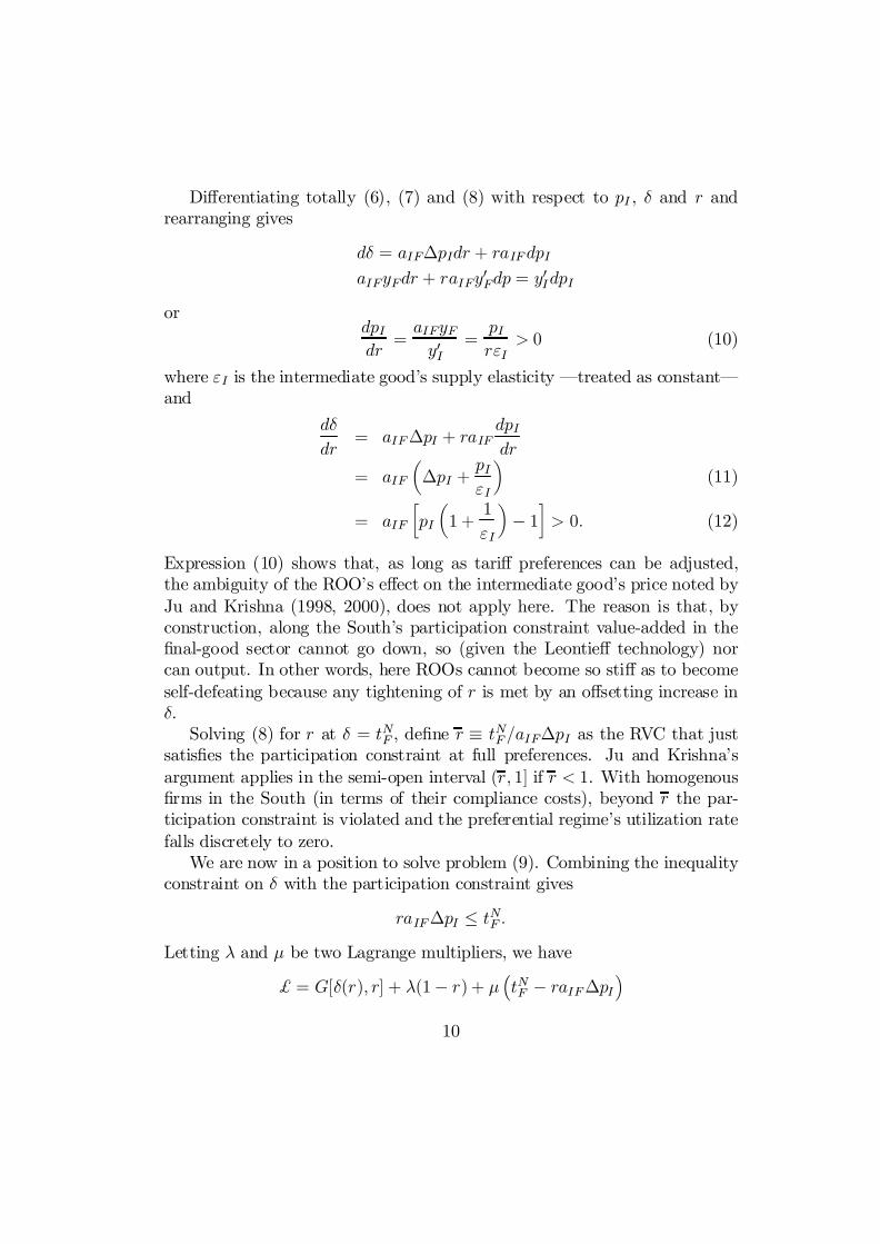
Di¤erentiating totally (6), (7) and (8) with respect to pI , ± and r andrearranging gives

d± = aIF¢pIdr + raIF dpIaIFyFdr + raIFy0Fdp = y0IdpI

ordpIdr =

aIFyFy0I

=pIr"I> 0 (10)

where "I is the intermediate good’s supply elasticity —treated as constant—and

d±dr

= aIF¢pI + raIFdpIdr

= aIFµ¢pI +

pI"I

¶(11)

= aIF·pI

µ1 +

1"I

¶¡ 1

¸> 0: (12)

Expression (10) shows that, as long as tari¤ preferences can be adjusted,the ambiguity of the ROO’s e¤ect on the intermediate good’s price noted byJu and Krishna (1998, 2000), does not apply here. The reason is that, byconstruction, along the South’s participation constraint value-added in the…nal-good sector cannot go down, so (given the Leontie¤ technology) norcan output. In other words, here ROOs cannot become so sti¤ as to becomeself-defeating because any tightening of r is met by an o¤setting increase in±.

Solving (8) for r at ± = tNF , de…ne r ´ tNF =aIF¢pI as the RVC that justsatis…es the participation constraint at full preferences. Ju and Krishna’sargument applies in the semi-open interval (r; 1] if r < 1. With homogenous…rms in the South (in terms of their compliance costs), beyond r the par-ticipation constraint is violated and the preferential regime’s utilization ratefalls discretely to zero.

We are now in a position to solve problem (9). Combining the inequalityconstraint on ± with the participation constraint gives

raIF¢pI · tNF :Letting ¸ and ¹ be two Lagrange multipliers, we have

$ = G[±(r); r] + ¸(1¡ r) + ¹³tNF ¡ raIF¢pI

´

10

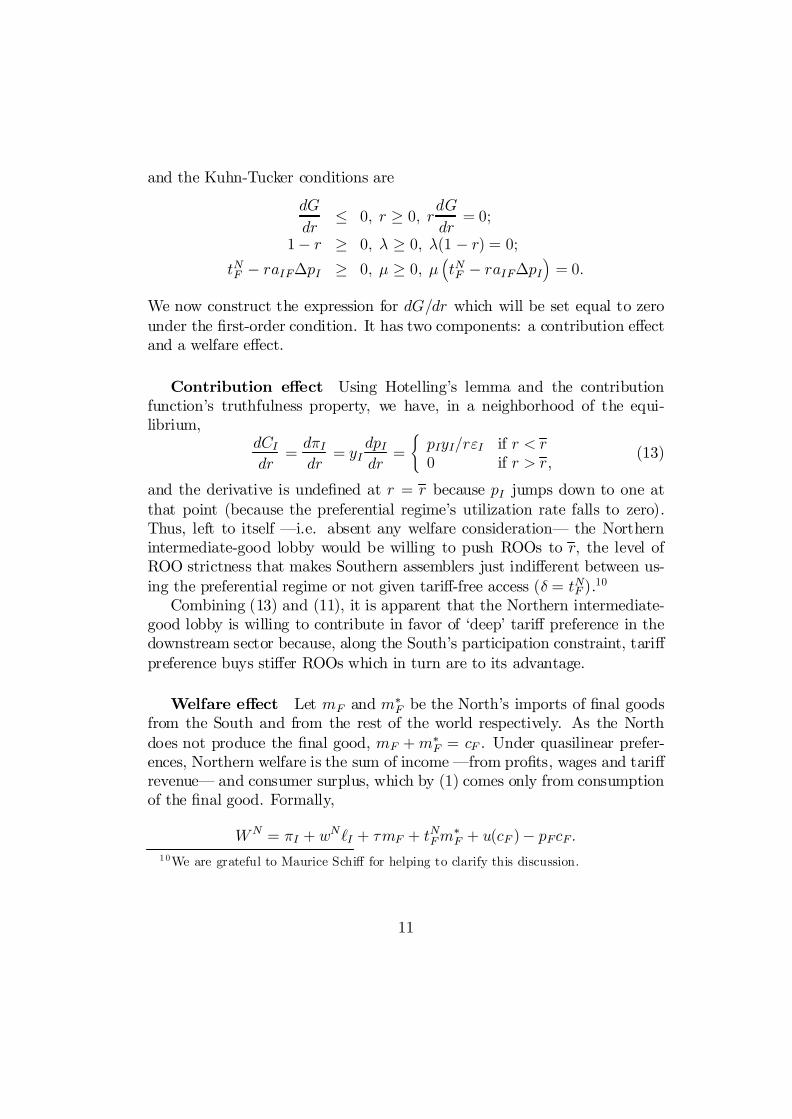
and the Kuhn-Tucker conditions are

dGdr

· 0; r ¸ 0; rdGdr

= 0;

1¡ r ¸ 0; ¸ ¸ 0; ¸(1 ¡ r) = 0;tNF ¡ raIF¢pI ¸ 0; ¹ ¸ 0; ¹

³tNF ¡ raIF¢pI

´= 0:

We now construct the expression for dG=dr which will be set equal to zerounder the …rst-order condition. It has two components: a contribution e¤ectand a welfare e¤ect.

Contribution e¤ect Using Hotelling’s lemma and the contributionfunction’s truthfulness property, we have, in a neighborhood of the equi-librium,

dCIdr

= d¼Idr

= yIdpIdr

=(pIyI=r"I if r < r0 if r > r; (13)

and the derivative is unde…ned at r = r because pI jumps down to one atthat point (because the preferential regime’s utilization rate falls to zero).Thus, left to itself —i.e. absent any welfare consideration— the Northernintermediate-good lobby would be willing to push ROOs to r; the level ofROO strictness that makes Southern assemblers just indi¤erent between us-ing the preferential regime or not given tari¤-free access (± = tNF ).10

Combining (13) and (11), it is apparent that the Northern intermediate-good lobby is willing to contribute in favor of ‘deep’ tari¤ preference in thedownstream sector because, along the South’s participation constraint, tari¤preference buys sti¤er ROOs which in turn are to its advantage.

Welfare e¤ect Let mF and m¤F be the North’s imports of …nal goods

from the South and from the rest of the world respectively. As the Northdoes not produce the …nal good, mF +m¤

F = cF . Under quasilinear prefer-ences, Northern welfare is the sum of income —from pro…ts, wages and tari¤revenue— and consumer surplus, which by (1) comes only from consumptionof the …nal good. Formally,

WN = ¼I + wN`I + ¿mF + tNFm¤F + u(cF )¡ pFcF :

1 0We are grateful to Maurice Schi¤ for helping to clarify this discussion.

11

As mF = yF (the South exports its entire …nal-good output to the North),m¤F = cF ¡mF = cF ¡ yF , so

WN = ¼I +wN`I + tNF cF ¡ ±yF + u(cF )¡ pFcF : (14)

Along the South’s participation constraint, p is constant and hence so isyF . Thus, treating pI and ± as endogenous variables along the problem’sconstraints,

dWN

dr = yIdpIdr ¡ yF

d±dr

=pIyIr"I

¡ aIF yF·pI

µ1 +

1"I

¶¡ 1

¸:

Using the fact that, by (7), aIFyF = yI=r, this becomes

dWN

dr=yIr

½pI"I

¡·pI

µ1 +

1"I

¶¡ 1

¸¾

= ¡yIr¢pI < 0: (15)

Combining the contribution and welfare e¤ects gives

dGN

dr= dCI

dr+ adW

N

dr= pIyIr"I

¡ ayIr¢pI

=pIyIr

Ã1"I

¡ a¢pIpI

!:

Under the …rst-order condition, this expression is set equal to zero, so

pI¢pI

= a"I: (16)

The second-order condition requires a"I > 1, which we assume to hold.11

1 1This assumption is not innocuous. The parameter a is, in our setting, the dollaramount that the intermediate-good lobby must contribute per equivalent-dollar of welfarereduction. As contributions are typically small relative to the distortionary costs of tradepolicies, a is likely to be smaller than one. Then "I , the elasticity of supply of intermediategoods, must be larger than one. When this assumption is violated, a corner solution occursat either r = 0 (no ROO) or r = r .

12

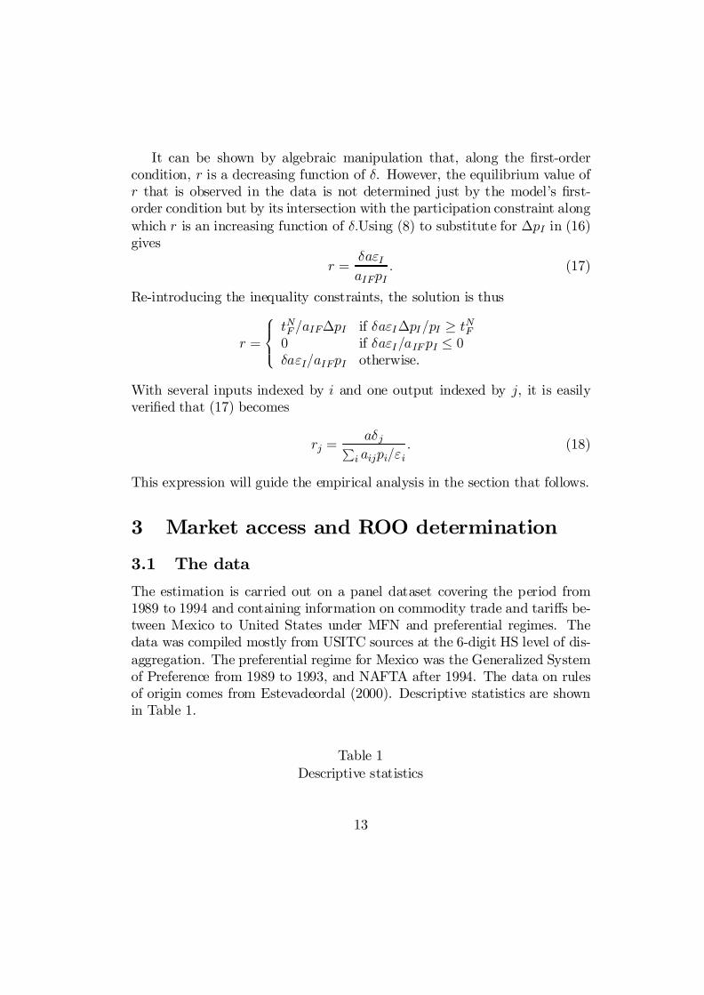
It can be shown by algebraic manipulation that, along the …rst-ordercondition, r is a decreasing function of ±. However, the equilibrium value ofr that is observed in the data is not determined just by the model’s …rst-order condition but by its intersection with the participation constraint alongwhich r is an increasing function of ±:Using (8) to substitute for ¢pI in (16)gives

r =±a"IaIFpI

: (17)

Re-introducing the inequality constraints, the solution is thus

r =

8><>:

tNF =aIF¢pI if ±a"I¢pI=pI ¸ tNF0 if ±a"I=aIF pI · 0±a"I=aIFpI otherwise.

With several inputs indexed by i and one output indexed by j, it is easilyveri…ed that (17) becomes

rj =a±jPi aijpi="i

: (18)

This expression will guide the empirical analysis in the section that follows.

3 Market access and ROO determination

3.1 The dataThe estimation is carried out on a panel dataset covering the period from1989 to 1994 and containing information on commodity trade and tari¤s be-tween Mexico to United States under MFN and preferential regimes. Thedata was compiled mostly from USITC sources at the 6-digit HS level of dis-aggregation. The preferential regime for Mexico was the Generalized Systemof Preference from 1989 to 1993, and NAFTA after 1994. The data on rulesof origin comes from Estevadeordal (2000). Descriptive statistics are shownin Table 1.

Table 1Descriptive statistics

13

3.2 Empirical estimationWe estimate two equations: a market-access one and a political one. Let jstand for a tari¤ line (at the HS6 level) and t for time measured in years. Theestimated system has a peculiar structure in the time dimension. Mexicanexports to the US ( yjt) and to the world (xjt) vary over time. So doesthe rate of preference (±jt), as NAFTA’s tari¤ reductions were phased inprogressively over a transition period (on this, see Estevadeordal 2000). Bycontrast, rules of origin (rj) were negotiated once and for all in the early1990s. Thus, the market-access equation must be estimated on panel datawhereas the political determination of ROOs must be estimated on a crosssection of tari¤ lines with the variables suggested by the model as likelydeterminants of ROOs, as of the 1990s.

We measure ROOs in two alternative ways. First, we use a vector ofbinary variables, each marking the presence of a speci…c ROO instrument(change of tari¤ heading, technical requirement etc.). Second, we use Es-tevadeordal’s synthetic index. Using both proxies provides a check on theconstruction of Estevadeordal’s index, as estimated coe¢cients should belarger in absolute value for instruments assigned a higher value in his index.

Thus, the market-access equations to be estimated is either

ln yjt = ®0t + ®1 ln xjt + ®2 ln ±jt + ®3rj + ujt (19)

where xjt stands for Mexican exports of good j to the rest of the world, ±jtis the rate of preference granted to good j in year t under NAFTA, rj isEstevadeordal’s (2000) index of ROO strictness, and ujt is an error term.Alternatively,

ln yjt = ®0t + ®1 lnxjt + ®2 ln ±jt +nX

k=1

e®krkj + ujt (20)

with a vector of n binary variables for the n legal forms of ROOs.We control for serial correlation in the time dimension by time e¤ects and

for unobserved industry characteristics by …xed e¤ects at the section level.As the estimation is carried out at the hs6 level of aggregation, we control forheteroskedasticity by using weighted least squares, the weight being Mexico’stotal exports. Expected signs and magnitudes in (19) are ®1 = 1; ®2 > 0;®3 < 0, and, in (20), e®k+1 < e®k < 0 if ROO type k + 1 is assigned a higher

14

value than ROO type k in Estevadeordal’s index.12

The political equation is based on (18) in log form. As values of ± duringthe phase-out period were determined simultaneously with rules of origin,we instrument for ± using its steady-state value ±j, the US MFN tari¤ (thelatest available value is for 2001).13 Thus,

ln rj = ¯0+ ¯1 lnÃ

X

iaijpi="i

!+ ¯2 ln ±j: (21)

1 2This equation can be justi…ed as follows. Consider a Mexican …nal-good exportermaximizing pro…ts by choice of a mixture of export destinations. Let y stand for thevalue added of exports to the US, x for the value added of exports to the rest of theworld, and let p be the relative net price in the US. Assume that the …rm produces outof a …xed pool of ressources R under a Constant Elasticity of Transformation technology(Powell and Gruen, 1962), i.e. x® + y® = R where ® is the inverse of the elasticity oftransformation. The value of R is itself determined in the previous stage of a two-stageoptimization problem. The second-stage problem is thus

maxx;y

x + py s.t. x® + y® = R:

The FOC yield y=x = p1=(®¡1) or

lny =1

® ¡ 1lnp + lnx;

a functional form close to (19). If this equation is roughly invariant across tari¤ lines,the elasticity of transformation between the US and the ROW can be retrieved fromthe parameter estimate on the tari¤ preference term, whereas the parameter estimate onexports to the ROW should be insigi…cantly di¤erent from one.

The interest of this formulation is that because of the curvature of the transformationsurface, the export mixture is an interior solution even when the participation constraintis binding (i.e. when p = 1), an observation that is largely true at the tari¤ line (althoughnot necessarily true at the …rm level). This framework can be easily extended to a three-dimensional choice in which exports to the US can be made under either the preferentialregime or the MFN one. If the choice between legal regimes for exports to the US involvesno e¢ciency consideration, the transformation surface can be represented as

x® + (yN AFTA + yMFN )® = R:

1 3We also tested an alternative formulation, namely e±j =P1

t=0 ¯ t±jt with ¯ = 0:9.Results were similar.

15

Alternatively, noting that, by (10)

pi"i

=raijyjy0i

=yiy 0i;

it follows that X

i

aijpi"i

=X

i

aijyiy0i;

so letting zj =Pi aijyi=y 0i, the equation to be estimated becomes

ln rj = ¯0 + ¯1 ln zj + ¯2 ln ±j + vj: (22)

where ¯0 = lna < 0 (if a < 1), ¯1 < 0; ¯2 = 1; vj is an error term, andzj =

Pi aijyi=y 0i is proxied (with measurement errors since y0i is unobserved)

byPi aijyi, the sum, over all goods i upstream of j, of the product of US

exports of good i to Mexico, yi, times the share aij of good i in good j’soutput.

Note that there is no endogeneity bias from the fact that zj is a linearcombination of intermediate-good exports from the US to Mexico that may bea¤ected by …nal-good exports from Mexico to the US because zj is calculatedas an average for three years before NAFTA’s entry into force, so the linkbetween the two types of trade ‡ows is tenuous at best. Thus, the system isrecursive and estimated as such.

As estevadeordal’s ROO index is a categorical variable which takes oninteger values between one and seven, the political equation is estimated asan ordered probit. As a result, direct quantitative interpretation of parameterestimates in terms of (22) is not possible. As the model assumes that ROOstake the form of a continuous RVC whereas actual ones are combinations ofdiscrete instruments, there is no way around this di¢culty.

As a robustness check, we split the sample of Mexican exports to theUS into …nal vs. intermediate and capital goods. As the logic of our modelapplies essentially to …nal goods exported by Mexico with intermediates im-ported from the US, the e¤ect of ROOs should be stronger for the sub-samplerestricted to …nal goods.

3.3 ResultsEstimation results are shown in Tables 2 and 3.

16

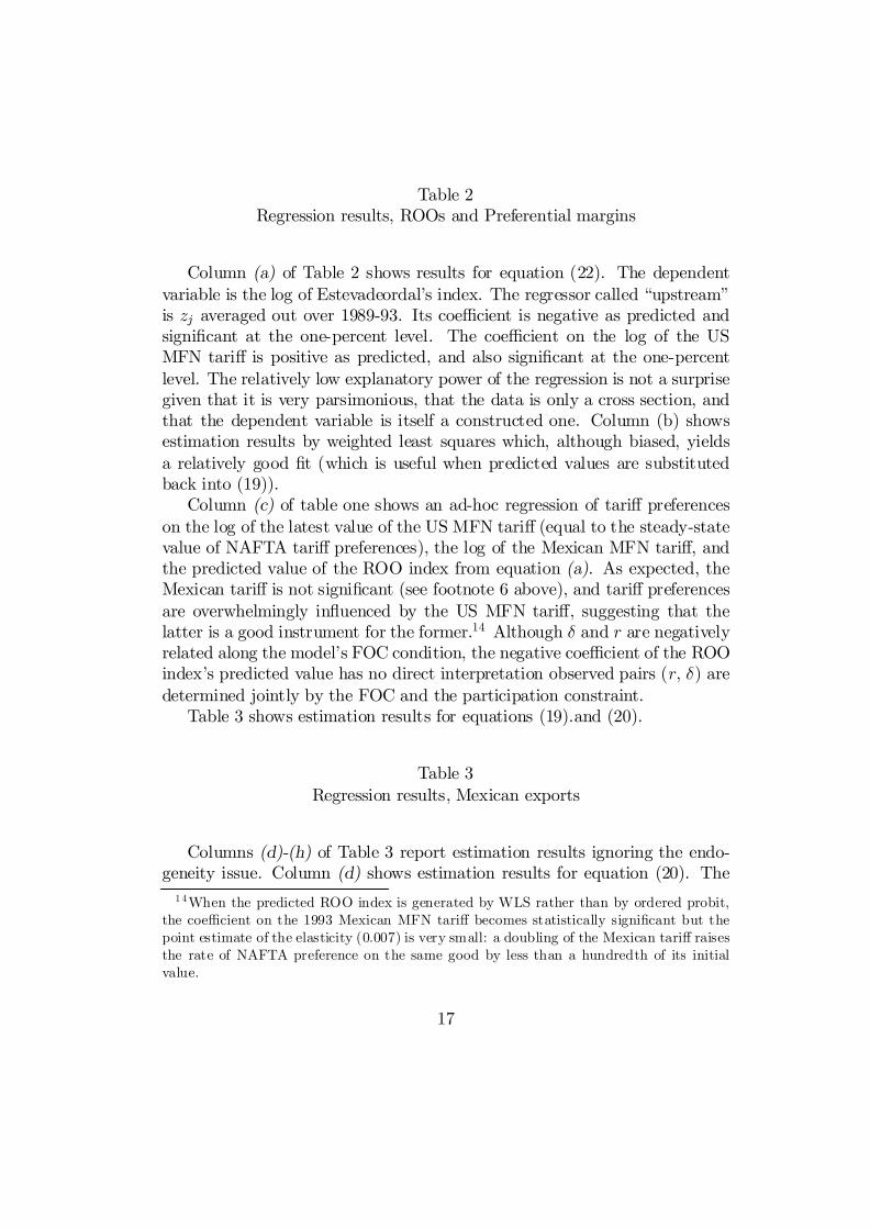
Table 2Regression results, ROOs and Preferential margins

Column (a) of Table 2 shows results for equation (22). The dependentvariable is the log of Estevadeordal’s index. The regressor called “upstream”is zj averaged out over 1989-93. Its coe¢cient is negative as predicted andsigni…cant at the one-percent level. The coe¢cient on the log of the USMFN tari¤ is positive as predicted, and also signi…cant at the one-percentlevel. The relatively low explanatory power of the regression is not a surprisegiven that it is very parsimonious, that the data is only a cross section, andthat the dependent variable is itself a constructed one. Column (b) showsestimation results by weighted least squares which, although biased, yieldsa relatively good …t (which is useful when predicted values are substitutedback into (19)).

Column (c) of table one shows an ad-hoc regression of tari¤ preferenceson the log of the latest value of the US MFN tari¤ (equal to the steady-statevalue of NAFTA tari¤ preferences), the log of the Mexican MFN tari¤, andthe predicted value of the ROO index from equation (a). As expected, theMexican tari¤ is not signi…cant (see footnote 6 above), and tari¤ preferencesare overwhelmingly in‡uenced by the US MFN tari¤, suggesting that thelatter is a good instrument for the former.14 Although ± and r are negativelyrelated along the model’s FOC condition, the negative coe¢cient of the ROOindex’s predicted value has no direct interpretation observed pairs (r, ±) aredetermined jointly by the FOC and the participation constraint.

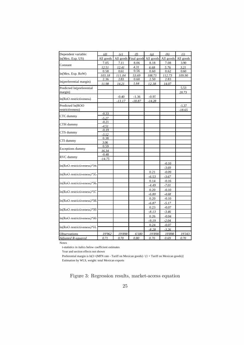
Table 3 shows estimation results for equations (19).and (20).

Table 3Regression results, Mexican exports

Columns (d)-(h) of Table 3 report estimation results ignoring the endo-geneity issue. Column (d) shows estimation results for equation (20). The

1 4When the predicted ROO index is generated by WLS rather than by ordered probit,the coe¢cient on the 1993 Mexican MFN tari¤ becomes statistically signi…cant but thepoint estimate of the elasticity (0.007) is very small: a doubling of the Mexican tari¤ raisesthe rate of NAFTA preference on the same good by less than a hundredth of its initialvalue.

17

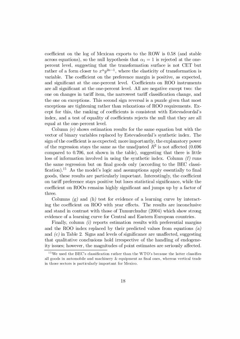
coe¢cient on the log of Mexican exports to the ROW is 0.58 (and stableacross equations), so the null hypothesis that ®1 = 1 is rejected at the one-percent level, suggesting that the transformation surface is not CET butrather of a form closer to x®y2®¡1; where the elasticity of transformation isvariable. The coe¢cient on the preference margin is positive, as expected,and signi…cant at the one-percent level. Coe¢cients on ROO instrumentsare all signi…cant at the one-percent level. All are negative except two: theone on changes in tari¤ item, the narrowest tari¤ classi…cation change, andthe one on exceptions. This second sign reversal is a puzzle given that mostexceptions are tightening rather than relaxations of ROO requirements. Ex-cept for this, the ranking of coe¢cients is consistent with Estevadeordal’sindex, and a test of equality of coe¢cients rejects the null that they are allequal at the one-percent level.

Column (e) shows estimation results for the same equation but with thevector of binary variables replaced by Estevadeordal’s synthetic index. Thesign of the coe¢cient is as expected; more importantly, the explanatory powerof the regression stays the same as the unadjusted R2 is not a¤ected (0.696compared to 0.706, not shown in the table), suggesting that there is littleloss of information involved in using the synthetic index. Column (f) runsthe same regression but on …nal goods only (according to the BEC classi-…cation).15 As the model’s logic and assumptions apply essentially to …nalgoods, these results are particularly important. Interestingly, the coe¢cienton tari¤ preference stays positive but loses statistical signi…cance, while thecoe¢cient on ROOs remains highly signi…cant and jumps up by a factor ofthree.

Columns (g) and (h) test for evidence of a learning curve by interact-ing the coe¢cient on ROO with year e¤ects. The results are inconclusiveand stand in contrast with those of Tumurchudur (2004) which show strongevidence of a learning curve for Central and Eastern European countries.

Finally, column (i) reports estimation results with preferential marginsand the ROO index replaced by their predicted values from equations (a)and (c) in Table 2. Signs and levels of signi…cance are una¤ected, suggestingthat qualitative conclusions hold irrespective of the handling of endogene-ity issues; however, the magnitudes of point estimates are seriously a¤ected.

1 5We used the BEC’s classi…cation rather than the WTO’s because the latter classi…esall goods in automobile and machinery & equipment as …nal ones, whereas vertical tradein those sectors is particularly important for Mexico.

18

suggesting that quantitative conclusions must be drawn carefully. Interest-ingly, the point estimates of the coe¢cients on preferences and ROOs bothgo up, suggesting that the e¤ect of both trade-policy instruments are under-estimated when endogeneity issues are ignored.

4 Concluding remarksTwo messages come out of our results. One is empirical, the other concep-tual. First, at the empirical level, NAFTA’s rules of origin seem to dilutethe bene…ts generated by preferential trade liberalization, in terms of marketaccess, for Mexico. This result, which is in conformity with the …ndings ofthe recent literature, suggests that ROOs should indeed be viewed as an eco-nomically sensitive item rather than a technical one in the agenda of bilateraltrade negotiations. Moreover, the e¤ect seems to be stronger for …nal goodsthan for intermediate ones, in conformity with what one would expect in amulti-stage production model where each stage is located according to theproduction stage’s factor intensity and the host country’ factor abundance.This result begs the question, why do Northern partners create policy instru-ments that put hurdles in a process that is economically e¢cient? One reasonmight be that ROOs are the price to pay for the acquiescence of Northern…nal-good producers threatened by Southern competition. However, many ofthe …nal-good assemblage activities undertaken by Southern ‘maquiladoras’are non-competing, making this explanation less than satisfactory.

The second point of our paper is about this issue. We use a standardmodel of endogenous trade policy —Grossman and Helpman’s common-agency model— to explore an alternative logic, namely that ROOs re‡ectpolitical pressure by Northern intermediate-good producers interested in cre-ating captive markets for their goods in the South. The logic is as follows.On the assumption that the Mexican side is on its “participation constraint”,i.e. that the rate of e¤ective protection conferred to Mexican …nal-good pro-ducers by the simultaneous use of tari¤ preferences and ROOs is just aboutzero, tari¤ preferences are the price to be paid for Mexican assemblers’ ac-quiescence to a system which forces them to buy US intermediate goods.Seen this way, as the model shows, preferences-cum-ROOs amount to a puretransfer from US taxpayers to intermediate-good producers, i.e. to a hiddenexport subsidy. Because export subsidies are in violation of any country’sobligations under the GATT, recourse to an indirect and ine¢cient substitute

19

instrument —ROOs— makes sense.Empirically, the model suggests the inclusion, among the right-hand side

variables of the second equation (ROO determination), of the product ofinput-output coe¢cients by US intermediate sales to Mexico. This somewhatunintuitive prediction provides a test of the approach’s validity, since it isdi¢cult to think of an alternative theoretical approach that would lead to theinclusion of that particular algebraic term. Empirical results are in strikingconformity with the model’s predictions. In sum, they suggest that the useof NAFTA to create a captive market for US intermediates was indeed oneof the forces shaping the agreement’s rules of origin.

References[1] Ansolobehere, Stephen; J. de Figuereido and James Snyder (2002),

“Why is There So Little Money in U.S. Politics?”; NBER working paper#9409.

[2] Anson, Jose, O. Cadot, A. Estevadeordal, J. de Melo, A. Suwa-Eisenmann and B. Tumurchudur (2003), “Rules of Origin in North-South Preferential Trading Arrangements with an Application toNAFTA”, mimeo, University of Lausanne.

[3] Cadot, Olivier, A. Estevadeordal, J. de Melo, A. Suwa-Eisenmann andB. Tumurchudur (2001), “Assessing the e¤ect of NAFTA’s rules of ori-gin”, mimeo, The World Bank.

[4] Carrère, Céline, and J. de Melo: “A Free-Trade Area of the Americas:Any Gains for the South?”; mimeo, University of Geneva.

[5] Dixit, Avinash, and G. Grossman (1982), “Trade and Protection withMultistage Production”; Review of Economic Studies 49, 583-594.

[6] Duttagupta, Rupa (2000), Intermediate Inputs and Rules of Origin–Implications for Welfare and Viability of Free Trade Agreements, Ph.Ddissertation, University of Maryland.

[7] — and A. Panagariya, (2002), “Free Trade Areas and Rules of Origin:Economics and Politics”, mimeo, University of Maryland.

20

[8] Estevadeordal, Antoni (2000), “Negotiating Preferential Market Access:The Case of the North American Free Trade Agreement”, Journal ofWorld Trade 34, 141-66.

[9] — and K. Suominen (2003), “Rules of Origin: A World Map and TradeE¤ects”, mimeo, IADB.

[10] Falvey, Rod. and G. Reed, (2000), Economic E¤ects of Rules of Origin,Weltwirtcha‡iches Archiv 143, 209-29.

[11] Grossman, Gene, and E. Helpman (1995), “The Politics of Free-TradeAgreements”; American Economic Review 85, 667-690.

[12] Hanson, Gordon (1996), “Localization Economies, Vertical Integration,and Trade” American Economic Review 86, 1266-1278.

[13] Ju, Jiandong and Kala Krishna (1998), “Firm Behaviour and MarketAccess in a Free Trade Area With Rules of Origin”, NBER WorkingPaper 6857.

[14] — (2002), “Regulation, Regime Switches and Non-Monotonicity whenNon-Compliance is an option: An Application to Content protectionand Preference”, forthcoming, Economics Letters.

[15] Krishna, Kala (2002), “Understanding Rules of Origin”, mimeo, 2002.

[16] — and A. Krueger (1995), “Implementing Free Trade Areas: Rules ofOrigin as Hidden Protection”, in A. Deardor¤, J. Levinsohn and R.Stern eds. New Directions in Trade Theory, 149-87.

[17] Krueger, Anne. (1997), “Free Trade Areas versus Customs Union”, Jour-nal of Development Economics 54, 169-97.

[18] Powell, Alan A. and F.H.G. Gruen (1962), “The Constant Elasticity ofTransformation Production Frontier and Linear Supply System”, Inter-national Economic Review 9, 315-328.

[19] Lloyd, Peter (1993), “A tari¤ Substitute for Rules of Origin in Free-Trade Areas”; World Economy 16, 699-712.

[20] Rodriguez, Peter (2001), “Rules of Origin with Multistage Production”;World Economy 24, 201-220.

21

[21] Sanguinetti, Pablo (2003) “Implementing rules of origin in the southerncone PTAS in Latin America”, paper presented at the IADB/CEPRworkshop on Rules of Origin, Paris, April 2003.

[22] Serra, Jaime, G. Aguilar and C. Hills, eds. (1996), Re‡ections on Region-alism: Report of the Study Group on International Trade; Washington,D.C.: Carnegie Endowment for International Peace press.

[23] Tumurchudur, Bolormaa (2004), “Rules of origin and market access inthe EU’s agreements with the CEECs”, mimeo, University of Lausanne(Ph.D dissertation work in progress).

[24] Yeats, Alexander J. (1998), “Does Mercosur’s Trade Performance RaiseConcerns about the E¤ects of Regional Trade Arrangements?” WorldBank Economic Review. 12,.1-28.

22

Figure 1: Descriptive StatisticsVariable Observations Mean Std. Dev. Min Max

Log Mex. pref. exports to US 21056 13.091 3.090 5.533 23.003Log Mex. exports to ROW 33943 11.817 2.963 -0.024 21.556RoO restr. index 42457 5.056 1.298 0.000 7.000Predicted Value RoO rest. ind. 39936 0.139 0.121 0.009 2.271Log Roo restr. index 43639 1.538 0.406 0.000 1.946Log pred. value of RoO rest. ind 39936 -2.373 0.955 -4.673 0.820Log (Pref. Margin + 1) 42062 0.025 0.050 -0.150 1.504Log (Pred. value of Pref. margin + 1) 38672 0.029 0.051 -0.047 1.180US MFN tariff 2001 42443 0.031 0.083 0.000 3.046Mex. MFN tariff 93 40804 0.153 0.158 0.000 2.820Log US MFN Tariff 2001 + 1 42443 0.028 0.058 0.000 1.398Log Mex. MFN tariff 1993 + 1 40804 0.137 0.085 0.000 1.340Chapter Dummy 43639 0.503 0.500 0 1Heading Dummy 43639 0.375 0.484 0 1Sub-Heading Dummy 43639 0.040 0.196 0 1Item Dummy 43639 0.000 0.019 0 1Exception Dummy 42822 0.266 0.442 0 1RVC Dummy 43639 0.434 0.496 0 1Pref. margin*94 4991 0.021 0.037 -0.118 0.747Pref. margin*95 4979 0.023 0.038 -0.041 0.972Pref. margin*96 5360 0.025 0.062 -0.139 1.831Pref. margin*97 5363 0.029 0.072 -0.080 2.777Pref. margin*98 5370 0.030 0.082 -0.001 3.244Pref. margin*99 5386 0.030 0.086 -0.001 3.500Pref. margin*00 5470 0.029 0.072 -0.014 2.828Pref. margin*01 5143 0.031 0.084 0.000 2.970

23

Figure 2: Regression results, ROO index and pref. margins

(a) (b) (c)Dep. var. (in log): ROO index ROO index Pref. marg.Estimation Ord. prob. WLS WLS

2.0634.02

-0.17 -0.30-11.11 -11.32

1.87 0.18 0.866.18 3.21 302.76

0.000.38-0.01-9.06

Observations 4'991 4'992 33'940Pseudo R-square 0.22R-square adj. 0.38 0.85Notes:

z-statistics (a) or t-statistics (b) in italics under coefficient estimateSection/time effects not shown (time effects only in (b))Preferential margin is ln[1+(MFN rate - Tariff on Mexican goods) / (1 + Tariff on Mexican goods)]

Constant

Predicted Value of ROO

Upstream

ln(1+US MFN tariff 2001)ln(Mexico MFN tariff 1992/1993)

24

(d) (e) (f) (g) (h) (i)All goods All goods Final goods All goods All goods All goods

7.05 7.11 8.06 8.18 7.08 3.9012.51 12.41 4.31 6.68 5.76 3.210.58 0.61 0.56 0.60 0.62 0.60

103.18 111.04 53.69 108.73 112.73 109.902.36 2.83 0.60 2.50 2.83

11.98 14.21 1.64 12.38 14.075.53

20.73-0.40 -1.36 -0.95

-13.17 -18.87 -14.28-1.37

-18.65-0.33-5.27-0.21-4.51-0.19-3.120.383.060.59

16.34-0.48

-14.75-0.10-3.69

0.21 -0.09-6.53 -3.670.14 -0.16

-4.49 -7.010.20 -0.10

-6.80 -4.680.20 -0.10

-6.87 -5.170.23 -0.07

-8.13 -3.460.26 -0.04

-9.19 -2.040.24 -0.07

-8.28 -3.26Observations 19'962 19'898 6'180 19'898 19'898 19'343 Adjusted R-squared 0.71 0.70 0.80 0.70 0.69 0.70Notes

t-statistics in italics below coefficient estimates Year and section effects not shown

Preferential margin is ln[1+(MFN rate - Tariff on Mexican goods) / (1 + Tariff on Mexican goods)]Estimation by WLS, weight: total Mexican exports

Exceptions dummy

RVC dummy

ln(Mex. Exp. RoW)

ln(preferential margin)

CTC dummy

CTH dummy

ln(RoO restrictiveness)*01

ln(RoO restrictiveness)*94

ln(RoO restrictiveness)*95

ln(RoO restrictiveness)*96

ln(RoO restrictiveness)*97

Dependent variable: ln(Mex. Exp. US)

ln(RoO restrictiveness)*98

ln(RoO restrictiveness)*99

ln(RoO restrictiveness)*00

Constant

ln(RoO restrictiveness)

Predicted ln(preferential margin)

Predicted ln(ROO restrictiveness)

CTS dummy

CTI dummy

Figure 3: Regression results, market-access equation

25