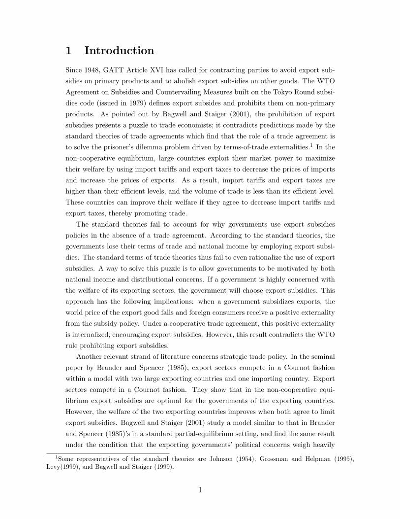
Import Tariffs and Export Subsidies in the WTO:

A Small-Country Approach

Tanapong Potipiti ∗

Chulalongkorn University

email: Tanapong.P@chula.ac.th

April 2006

Abstract

This paper develops a simple small-country model to explain why the WTO pro-

hibits export subsidies but allows import tariffs. Governments choose protection rates

(import tariffs/export subsidies) to maximize a weighted sum of social welfare and

lobbying contributions. While transportation costs decrease due to the progress of

trade liberalization and lower transportation costs, import-competing sectors decline

but export industries grow. In the growing export industries, the surplus generated by

protection is eroded by new entrants. Therefore, the rent that the governments gain

from protecting the export sectors by using export subsidies is small. On the other

hand, in the import-competing sectors, capital is sunk and no new entrants erode the

protection rent. Therefore, the governments can get large political contributions from

protecting these import-competing sectors. We show that under fast capital mobility,

the governments with a high bargaining power are better off from a trade agreement

that allows import tariffs but prohibits export subsidies.

∗I am grateful to Robert Staiger, Yeon-Cho Che, John Kennan, Bijit Bora, Kiriya Kulkolkarn and partic-ipants at the seminar in the WTO for helpful comments. I thank the WTO for financial support.

1 Introduction

Since 1948, GATT Article XVI has called for contracting parties to avoid export sub-

sidies on primary products and to abolish export subsidies on other goods. The WTO

Agreement on Subsidies and Countervailing Measures built on the Tokyo Round subsi-

dies code (issued in 1979) defines export subsides and prohibits them on non-primary

products. As pointed out by Bagwell and Staiger (2001), the prohibition of export

subsidies presents a puzzle to trade economists; it contradicts predictions made by the

standard theories of trade agreements which find that the role of a trade agreement is

to solve the prisoner’s dilemma problem driven by terms-of-trade externalities.1 In the

non-cooperative equilibrium, large countries exploit their market power to maximize

their welfare by using import tariffs and export taxes to decrease the prices of imports

and increase the prices of exports. As a result, import tariffs and export taxes are

higher than their efficient levels, and the volume of trade is less than its efficient level.

These countries can improve their welfare if they agree to decrease import tariffs and

export taxes, thereby promoting trade.

The standard theories fail to account for why governments use export subsidies

policies in the absence of a trade agreement. According to the standard theories, the

governments lose their terms of trade and national income by employing export subsi-

dies. The standard terms-of-trade theories thus fail to even rationalize the use of export

subsidies. A way to solve this puzzle is to allow governments to be motivated by both

national income and distributional concerns. If a government is highly concerned with

the welfare of its exporting sectors, the government will choose export subsidies. This

approach has the following implications: when a government subsidizes exports, the

world price of the export good falls and foreign consumers receive a positive externality

from the subsidy policy. Under a cooperative trade agreement, this positive externality

is internalized, encouraging export subsidies. However, this result contradicts the WTO

rule prohibiting export subsidies.

Another relevant strand of literature concerns strategic trade policy. In the seminal

paper by Brander and Spencer (1985), export sectors compete in a Cournot fashion

within a model with two large exporting countries and one importing country. Export

sectors compete in a Cournot fashion. They show that in the non-cooperative equi-

librium export subsidies are optimal for the governments of the exporting countries.

However, the welfare of the two exporting countries improves when both agree to limit

export subsidies. Bagwell and Staiger (2001) study a model similar to that in Brander

and Spencer (1985)’s in a standard partial-equilibrium setting, and find the same result

under the condition that the exporting governments’ political concerns weigh heavily

1Some representatives of the standard theories are Johnson (1954), Grossman and Helpman (1995),Levy(1999), and Bagwell and Staiger (1999).

1

on producer surplus. Furthermore, they show that although the exporting government

gains when limiting export subsidies, the outcome is inefficient from a global perspec-

tive. In the efficient outcome, export subsidies should be promoted, and the importing

country should transfer income to the exporting countries.

The studies discussed above are based on large-country models. Trade agreements

are instruments to solve externality problems among the governments of large coun-

tries. Another strand of literature argues that trade agreements can be used as a

commitment device to help a government enhance its credibility and solve domestic

time-inconsistency problems (see, for example, Staiger and Tabellini (1987), Tornell

(1991), Maggi and Rodriguiez-Clare (1998) and Mitra (2002)). These models provide

a rationale for the government of a small country to commit to a free trade agreement

and eliminate both tariffs and export subsidies.

Maggi and Rodriguiez-Clare (2005a and 2005b) have developed a model in which

trade agreements are motivated by both terms-of-trade and domestic commitment prob-

lems. Their model is novel in the following aspects: (i) they allow the agreement to

be incomplete and may specify only tariff and export subsidy ceilings rather than the

exact levels of tariffs and export subsidies2 and (ii) lobbying occurs in two stages – when

the agreement is designed3 (ex-ante lobbying) and when tariff and export subsidy rates

are selected by each government subject to the restrictions imposed by the agreement

(ex-post lobbying). In this model, they show that if the ex-post lobbying is stronger

than the ex-ante lobbying, the optimal trade agreement is incomplete, and it limits

both import tariffs and export subsidies.

The existing models have succeeded in explaining various aspects of trade agree-

ments. However they fail to account for the following asymmetric treatment of import

tariffs and export subsidies in the WTO. In the WTO, a country may choose their

own tariff binding level in exchange for concessions. On the contrary, export subsidies

are completely prohibited with few exceptions. In this paper, we propose a simple

small-country model using the commitment approach to explain this asymmetry.

The paper is organized as follows. Sections 2 and 3 describe the basic story and

the basic model, respectively. In section 4, we study how a government values a tariff

prohibition agreement and an export subsidy prohibition agreement differently, and

under what conditions it is optimal for the government to join an agreement that

prohibits only export subsidies. The last section concludes.

2An agreement is considered complete if it specifies the exact levels of tariffs and export subsidies.3For example, if the agreement is incomplete, in this stage, special interest groups might lobby for the

values of the tariff and export subsidy ceilings.

2

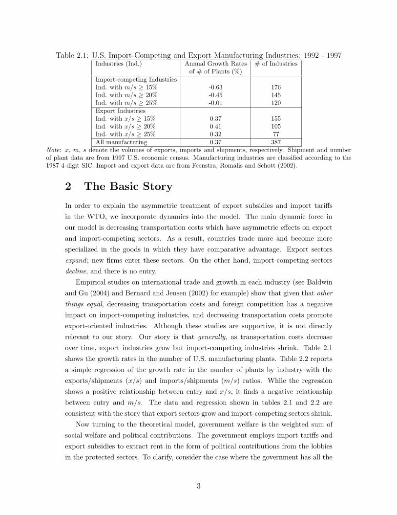
Table 2.1: U.S. Import-Competing and Export Manufacturing Industries: 1992 - 1997Industries (Ind.) Annual Growth Rates # of Industries

of # of Plants (%)Import-competing IndustriesInd. with m/s ≥ 15% -0.63 176Ind. with m/s ≥ 20% -0.45 145Ind. with m/s ≥ 25% -0.01 120Export IndustriesInd. with x/s ≥ 15% 0.37 155Ind. with x/s ≥ 20% 0.41 105Ind. with x/s ≥ 25% 0.32 77All manufacturing 0.37 387

Note: x, m, s denote the volumes of exports, imports and shipments, respectively. Shipment and numberof plant data are from 1997 U.S. economic census. Manufacturing industries are classified according to the1987 4-digit SIC. Import and export data are from Feenstra, Romalis and Schott (2002).

2 The Basic Story

In order to explain the asymmetric treatment of export subsidies and import tariffs

in the WTO, we incorporate dynamics into the model. The main dynamic force in

our model is decreasing transportation costs which have asymmetric effects on export

and import-competing sectors. As a result, countries trade more and become more

specialized in the goods in which they have comparative advantage. Export sectors

expand ; new firms enter these sectors. On the other hand, import-competing sectors

decline, and there is no entry.

Empirical studies on international trade and growth in each industry (see Baldwin

and Gu (2004) and Bernard and Jensen (2002) for example) show that given that other

things equal, decreasing transportation costs and foreign competition has a negative

impact on import-competing industries, and decreasing transportation costs promote

export-oriented industries. Although these studies are supportive, it is not directly

relevant to our story. Our story is that generally, as transportation costs decrease

over time, export industries grow but import-competing industries shrink. Table 2.1

shows the growth rates in the number of U.S. manufacturing plants. Table 2.2 reports

a simple regression of the growth rate in the number of plants by industry with the

exports/shipments (x/s) and imports/shipments (m/s) ratios. While the regression

shows a positive relationship between entry and x/s, it finds a negative relationship

between entry and m/s. The data and regression shown in tables 2.1 and 2.2 are

consistent with the story that export sectors grow and import-competing sectors shrink.

Now turning to the theoretical model, government welfare is the weighted sum of

social welfare and political contributions. The government employs import tariffs and

export subsidies to extract rent in the form of political contributions from the lobbies

in the protected sectors. To clarify, consider the case where the government has all the

3

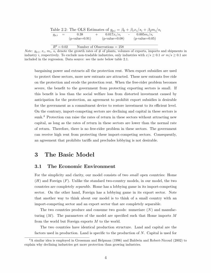
Table 2.2: The OLS Estimates of gp,i = β0 + β1xi/si + β2mi/si

gp,i = 0.38 + 0.017xi/si - 0.005mi/si

(p-value=0.91) (p-value=0.08) (p-value=0.05)

R2 = 0.02 Number of Observations = 258Note: gp,i, xi, mi, si denote the growth rates of # of plants, volumes of exports, imports and shipments inindustry i, respectively. To exclude non-tradable industries, only industries with x/s ≥ 0.1 or m/s ≥ 0.1 areincluded in the regression. Data source: see the note below table 2.1.

bargaining power and extracts all the protection rent. When export subsidies are used

to protect these sectors, more new entrants are attracted. These new entrants free ride

on the protection and erode the protection rent. When the free-rider problem becomes

severe, the benefit to the government from protecting exporting sectors is small. If

this benefit is less than the social welfare loss from distorted investment caused by

anticipation for the protection, an agreement to prohibit export subsidies is desirable

for the government as a commitment device to restore investment to its efficient level.

On the contrary, import-competing sectors are declining and capital in these sectors is

sunk.4 Protection can raise the rates of return in these sectors without attracting new

capital, as long as the rates of return in these sectors are lower than the normal rate

of return. Therefore, there is no free-rider problem in these sectors. The government

can receive high rent from protecting these import-competing sectors. Consequently,

an agreement that prohibits tariffs and precludes lobbying is not desirable.

3 The Basic Model

3.1 The Economic Environment

For the simplicity and clarity, our model consists of two small open countries: Home

(H) and Foreign (F ). Unlike the standard two-country models, in our model, the two

countries are completely separable. Home has a lobbying game in its import-competing

sector. On the other hand, Foreign has a lobbying game in its export sector. Note

that another way to think about our model is to think of a small country with an

import-competing sector and an export sector that are completely separable.

The two countries produce and consume two goods: numeriare (N) and manufac-

turing (M). The parameters of the model are specified such that Home imports M

from the world but Foreign exports M to the world.

The two countries have identical production structure. Land and capital are the

factors used in production. Land is specific to the production of N . Capital is used for

4A similar idea is employed in Grossman and Helpman (1996) and Baldwin and Robert-Nicoud (2002) toexplain why declining industries get more protection than growing industries.

4

both the production of N and M . Each country is endowed with k units of capital and

l units of land. The marginal product of capital in the production of N is:

f(kN ; lN = l) ≡ α− γkN

where kN and lN are, respectively, the levels of capital and land employed in the

production of N . The term γ is the slope of the demand for capital in sector N . The

total rent on land is:

Rl ≡kN∫0

f(t)dt− f(kN )kN =γk2

N

2.

Manufacturing production uses only capital. One unit of capital is required to produce

one unit of M .

The demand for M (di) and the consumer surplus (csi) of country i ∈ H,F from

consuming M are:

di(pi) = νi − pi and csi(pi) =(νi − pi)2

2

where pi is the local price of M in country i. We assume that νH is sufficiently high

and νF is sufficiently low that Home imports M and Foreign exports M . The local

price pi is defined as

pH ≡ pH + τH = (p + ζ) + τH (3.1)

pF ≡ pF + τF = (p− ζ) + τF (3.2)

where pi is the price of M in country i under free trade, τH and τF are, respectively, the

import tariff in Home and export subsidy in Foreign, p is the price of M in the world

market, and ζ is the cost of transporting M between the world market and the two

countries. As in standard economic geography models, we assume that the numeriare

is traded freely and is transported costlessly. The role of the transportation cost ζ is

crucial in our model and will be discussed in section 3.3. The amount of M imported

by country i is the difference between its domestic demand and supply:

imi(pi) = di(pi)− xi

where xi is the amount of capital employed in sector M in country i.

The social welfare of country i (ωi) is defined as:

ωi ≡ Ril + ki

Nf(kiN ) + pixi + csi(pi) + imi(pi)τ i (3.3)

where yi is the value of y in country i. The RHS of (3.3) is the sum of the return

5

on land, the producer surplus, the consumer surplus and the tariff revenue. Using the

capital market clearing condition: xi + kiN = k, (3.1) and (3.2), we can express ωi as a

function of xi and pi; ωi = ωi(xi, pi; νi, p, ζ).

3.2 The Lobbying Game

3.2.1 The Structure of the Game

In each country i ∈ H,F, a lobbying game is played by the government, the capitalists

and the lobbies formed by capitalists in sector M . The structure of the games in the

two countries is identical.

As a normalization, the length of the game is 1. Let t ∈ [0, 1] be the time index of

the game. For simplicity, we assume no payoff discounting overtime. The world price

p is constant for the whole game. However, the local price under free trade (pi) may

change due to the change in the transportation cost ζ, as shown in (3.1) and (3.2).

At time t = 0, each capitalist allocates all his capital in a sector. After capital is

allocated, a lobby is formed in sector M . No lobby is formed in sector N . In country i,

the lobby and the government negotiate for protection rate τ i and political contribution

ci. The protection rate τ i is set and unchanged for the whole game. Then, the lobby

pays the political contribution and no more contributions will be paid in the game.

In period t ∈ (0, 1− θ), goods are produced and traded. At time t = 1− θ, capital

can be moved from sector N to sector M in order to seek a higher rate of return. On

the other hand, once capital is employed in sector M , it is sunk and stays there, forever.

Therefore, capital cannot move from sector M to sector N . The term θ ∈ (0, 1] can

be interpreted as the speed of capital movement; it is negatively related to adjustment

costs of capital. This capital movement is the main difference between our model and

Maggi and Rodriguiez-Clare (1998)’s. In Maggi and Rodriguiez-Clare (1998), capital

cannot move across sectors after the protection rate is announced. Several empirical

studies show that there exists a strong relationship between the dynamic of an sector

and its protection level.5

In period t ∈ (1−θ, 1], goods are produced and traded. There is no capital movement

in this period. The game ends at t = 1.

For notational convenience, we define period 0 as the period where t = 0, period 1

as the period where t ∈ (0, 1− θ) and period 2 as the period where t ∈ [1− θ, 1].6 With

this notation, the game can be summarized as:

5Hufbauer and Rosen (1986), Hufbauer, Berliner and Elliot (1986), and Ray (1991) document that de-clining US industries receive more protections than the other industries. Glismann and Weiss (1980) findthat the growth rates of industry income are negatively correlated with the level of protection in Germanybetween 1880 and 1978.

6As θ → 0,period 2 disappears and our model becomes a special case of Maggi and Rodriguiez-Clare(1998).

6

• Timing

- In period 0, capital is allocated in each sector.

- In period 1, a lobby is formed in sector M of each country. The government

and the lobby bargain over the protection rate and political contributions.

The protection rate is set and unchanged until the end of the game. The

lobby pays the political contribution. Trade and production start.

- In period 2, capital may move from sector N to sector M to seek a higher

rate of return.

• Other assumptions

- The lengths of periods 0, 1 and 2 are 0, θ and 1− θ, respectively.

- Capital in sector M is sunk: xi1 ≥ xi

2. Note that a subscript denotes a time

period.

3.2.2 Payoffs

In this section, we define the payoff of each player. We begin with the capitalists. The

capitalists are highly concentrated and account for a negligible in the population. Each

capitalist can allocate his capital in one sector. Because each capitalist is so rich, his

utility from consuming non-numeriare goods and the government transfer is negligible.

A capitalist, therefore, maximizes his utility by allocating all his capital in the sector

with the highest rate of return.

The payoff of the lobby in country i, formed by the capitalists in sector M in period

1, is its net return on its sunk capital (Λi):

Λi ≡ (1− θ)pi1x

i1 + θpi

2xi1 − cixi

1. (3.4)

The government of country i maximizes the weighted sum of social welfare and

political contributions; its payoff is

Ωi ≡ (1− θ)ωi(xi1, p

i1) + acixi

1 + θωi(xi2, p

i2). (3.5)

The first and the last terms on the RHS are the social welfare in periods 1 and period 2,

respectively. The term ci is the political contribution per unit of capital and the term

cixi1 is the total contribution that the government gets from the lobby in sector M .

The term a ≥ 0 is the weight that the government puts on the political contribution

relative to the social welfare.7

7For simplicity, we assume that the two governments put the same weight on political contributions.

7

3.3 Transportation Costs, Growth of Import-competing

and Export Sectors, and Free Riders

In this section, we discuss the crucial role of the transportation cost ζ. As mentioned

above, the main difference between the export sector (in F ) and the import-competing

sector (in H) is that the export sector is expanding but the import-competing sector is

not. To have such an outcome, we assume a drop in the transportation cost in period

2: ζ2 < ζ1. The drop in transportation cost has asymmetric effects on the growth rates

of the import-competing and export sectors.8

The change in the transportation cost affects the rate of return of capital in the

manufacturing according to the following equations:

rH1 = p + ζ1 + τH(.)− cH(.) and rF

1 = p− ζ1 + τF (.)− cF (.)

rH2 = p + ζ2 + τH(.) and rF

2 = p− ζ2 + τF (.).

where rit is the rate of return of capital in sector M , in country i and in period t. The

terms p and ζt are exogenous. The political contribution ci and the protection rate τ i

are determined endogenously. In period 1, the rate of return of capital is the local price

(p+ ζ1 + τ i) minus the political contribution (ci). In period 2, the rate of return is just

the local price because there is no political contribution paid in this period.

The change in the rate of return in sector M in country i ∈ H,F between periods

1 and 2 is

∆rH = cH(.) + ∆ζ and ∆rF = cF (.)−∆ζ

where ∆y = y2 − y1. Capital moves from sector M to sector N if and only if ∆ri > 0.

Because the political contribution is always positive (ci > 0), ∆ζ < 0 implies that

∆rF > 0 and the growth in this sector is positive; there is always new capital moving

to this sector, in period 2. It is worth emphasizing that the owners of capital moved to

sector M , in period 2, free ride on the protection without participating in the lobbying.

On the other hand, whether the import-competing sector in H grows or not depends

on whether cH(.)+∆ζ is greater or less than 0. We focus on the case where ∆ζ < −cH(.)

and ∆rH < 0. Under these conditions, there is no incentive for new capital to move in

and free ride on the protection, in period 2. Moreover, capital cannot move out because

it is sunk. All capitalists that benefit from the protection invest their capital in this

sector in period 1 and pay for the protection.

Figure 3.3 shows the growth of capital in the import-competing sector in H and that

in the export sector in F . The solid line shows the growth of the import-competing

8Other potential exogenous forces that can drive similar outcomes are technological improvement in theexport sector and the progress of tariff reductions that decreases the prices of imports relative to the pricesof exports.

8

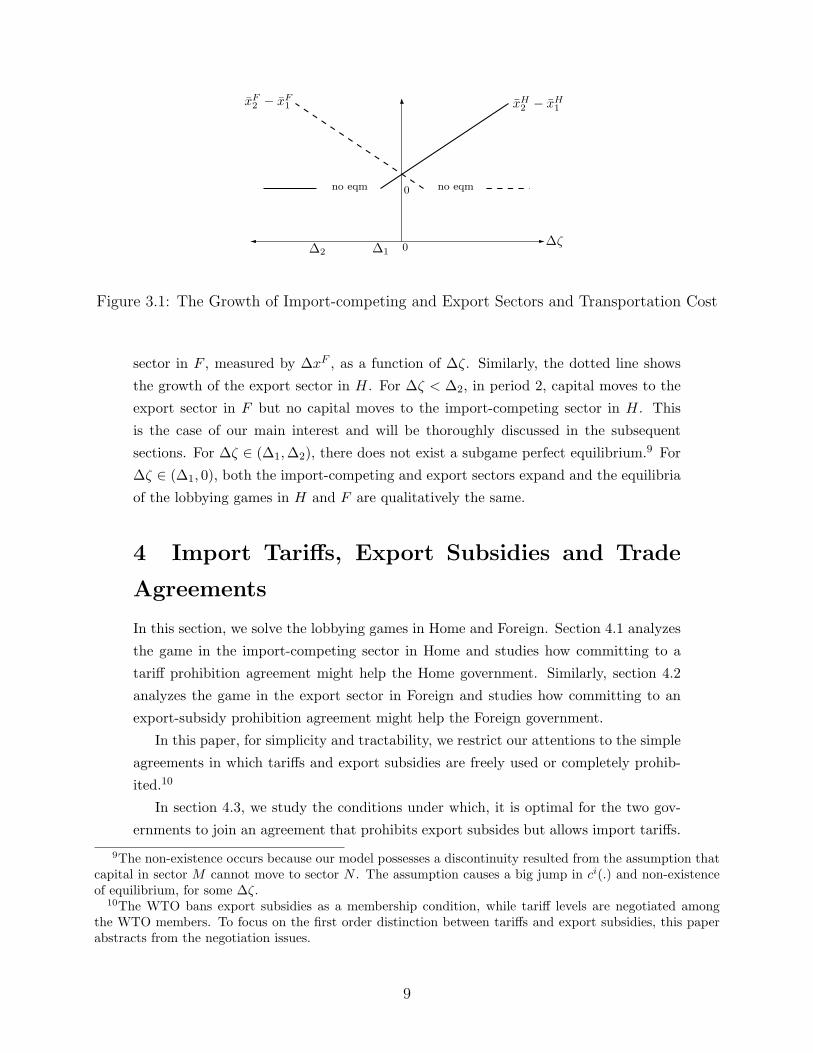
0

∆1∆2 0∆ζ

xH2 − xH

1xF

2 − xF1

no eqm no eqm

Figure 3.1: The Growth of Import-competing and Export Sectors and Transportation Cost

sector in F , measured by ∆xF , as a function of ∆ζ. Similarly, the dotted line shows

the growth of the export sector in H. For ∆ζ < ∆2, in period 2, capital moves to the

export sector in F but no capital moves to the import-competing sector in H. This

is the case of our main interest and will be thoroughly discussed in the subsequent

sections. For ∆ζ ∈ (∆1,∆2), there does not exist a subgame perfect equilibrium.9 For

∆ζ ∈ (∆1, 0), both the import-competing and export sectors expand and the equilibria

of the lobbying games in H and F are qualitatively the same.

4 Import Tariffs, Export Subsidies and Trade

Agreements

In this section, we solve the lobbying games in Home and Foreign. Section 4.1 analyzes

the game in the import-competing sector in Home and studies how committing to a

tariff prohibition agreement might help the Home government. Similarly, section 4.2

analyzes the game in the export sector in Foreign and studies how committing to an

export-subsidy prohibition agreement might help the Foreign government.

In this paper, for simplicity and tractability, we restrict our attentions to the simple

agreements in which tariffs and export subsidies are freely used or completely prohib-

ited.10

In section 4.3, we study the conditions under which, it is optimal for the two gov-

ernments to join an agreement that prohibits export subsides but allows import tariffs.

9The non-existence occurs because our model possesses a discontinuity resulted from the assumption thatcapital in sector M cannot move to sector N . The assumption causes a big jump in ci(.) and non-existenceof equilibrium, for some ∆ζ.

10The WTO bans export subsidies as a membership condition, while tariff levels are negotiated amongthe WTO members. To focus on the first order distinction between tariffs and export subsidies, this paperabstracts from the negotiation issues.

9

4.1 Import Tariffs and Import-Tariff Prohibition Agree-

ments

In this section, we study how the Home government might gain from an agreement to

prohibit tariffs. We first solve the lobbying game in the absence of tariff agreements.

Then, we solve the game under a tariff prohibition agreement and find the conditions

under which the government gains by committing to the agreement.

4.1.1 Import Tariffs in the Absence of Tariff Agreements

Now we are ready to solve the lobbying game in the import-competing sector of Home

in the absence of tariff agreements. Throughout the paper, we restrict our attention to

interior equilibria in which the levels of capital in all sectors are always positive. To

have such interior equilibria, we assume that the marginal productivity of capital in the

numeriare sector is not too high or too low and the weight that the government puts

on political contributions is not too high:

f(0) > p + ζ1, p− ζ1 ≥ f(k) ≥ 0 and γ ≥ a > 0. (A1)

Because good M is imported, its local price in period i is:

pFi = pF

i + τF = p + ζi + τF and pF1 > pF

2 .

As mention in the previous section, we assume that the transportation cost ζ drops

sufficiently fast that the rate of return on capital in sector M declines and no capital

moves to sector M in period 2. Particularly,

ζ2 − ζ1 ≤ ∆2 ≤ 0 (A2)

where

p + ζ1 −∆2 =2(p + ζ1)(γ − a)(1− θ) + a(1 + σ)f(k)

2γ(1− θ)− a(1− σ − 2θ)

This assumption ensures that no capital moves to sector M in period 2.

The lobbying game is solved by backward induction. In period 2, we suppose (and

will verify) that xH2 = xH

1 in equilibrium – no capital moves from the numeriare sector

to the manufacturing sector in period 2.

In period 1, after capital is allocated, xH1 is known. The lobby bargains with the

government for the tariff rate τH and political contribution cH . The bargaining subgame

is modeled as a Nash bargaining game in which the status quo is that the government

chooses free trade and the lobby pays no contributions. The government’s and the

lobby’s bargaining powers are σ and 1− σ, respectively. They choose the tariff rate to

10

maximize their joint surplus. The surplus is then split with respect to their bargaining

powers.

The government and the lobby pick the optimal protection rate τH(xH1 ) such that:

τH(xH1 ) = arg max

τH

(1− θ)ωH(xH1 , pH

1 + τH) +

θωH(xH2 , pH

2 + τH) + a[(1− θ)(pH1 + τH) + θ(pH

2 + τH)]xH1 . (4.3)

Note that y denotes the value of y in the subgame perfect equilibrium. From (3.5)

and (3.4), the term being maximized is the joint surplus of the two bargaining parties.

Solving the optimization by using xH1 = xH

2 , we obtain:

τH(xH1 ) = axH

1 . (4.4)

The optimal tariff rate is increasing in xH1 and a. The larger the values of xH

1 and a,

the higher the marginal gain from the tariff. Under Nash bargaining, the contribution

(cH) that the government receives from the protection is:

cH(xH1 ) = (1− σ)

∆H(xH1 , τH∗)

axH1

+ στH∗ (4.5)

where τH∗ ≡ τH(xH1 ). The term ∆H(.)/axH

1 is the adjusted welfare loss per unit

of capital generated by the tariff τH∗. The last τH∗ in this equation is the lobby’s

willingness to pay for the protection.

The welfare loss from the protection ∆H(xH1 , τH∗) is the difference between the free

trade welfare and the welfare under the protection:

∆H(xH1 , τH∗) ≡ (1− θ)[ωH(xH

1 , pH1 )− ωH(x1, p

H1 + τH∗)] +

θ[ωH(xH2 (xH

1 , 0), pH1 )− ωH(xH

2 (xH1 , τH∗), pH

2 + τH∗)], (4.6)

where xH2 (xH

1 , τH) is the level of capital in sector M in period 2 as a function of xH1

and τH in the subgame perfect equilibrium. Simplifying and using the supposition that

no capital moves to sector M in period 2 (xH2 (xH

1 , τH∗) = xH2 (xH

1 , 0) = xH1 ), we have:

∆H(xH1 , τH∗) =

τH∗2

2. (4.7)

Substituting (4.4) and (4.7) into (4.5), we obtain:

cH(xH1 ) =

a(1 + σ)xH1

2. (4.8)

11

The total gain for the government from protecting the import-competing sector is:

gH(xH1 ) ≡ (cH(xH

1 )− ∆H(xH1 , τH∗)

axH1

)xH1 =

σaxH2

1

2. (4.9)

In period 0, capital is allocated in sectors N and M such that the rates of return in

the two sectors are equal. Under the supposition that xH2 (xH

1 , τH∗) = xH1 , the levels of

capital in the two sectors are determined by:

(1− θ)f(k − xH1 ) + θf(k − xH

1 ) = (1− θ)pH1 + θpH

2 + τH(xH1 )− cH(xH

1 ) (4.10)

The LHS and the RHS are the total (periods 1 and 2) return on capital in sectors N

and M , respectively. Solving (4.10) for xH1 , we have:

xH1 =

(1− θ)pH1 + θpH

2 − f(k)2γ − a(1− σ)

. (4.11)

The government welfare under the lobbying game is:

ΩH = (1− θ)ωH(xH1 , pH

1 + τH∗) + θωH(xH1 , pH

2 + τH∗) + acH(xH1 )xH

1 . (4.12)

Finally, we have to verify the supposition that xH2 (xH

1 , τH∗) = xH2 (xH

1 , 0) = xH1 . We

need to show that there is no incentive for capital in sector N to move to sector M in

period 2:

f(k − xH1 ) ≥ pH

2 + τH∗. (4.13)

This condition can be verified by using (4.4), (4.11) and (A2). Because of sunk capital

in sector N , the rates of return on capital in sectors N and M are not equalized; the

rate of return in sector N is higher than that in sector M . Importantly, the protection

raises only the rate of return in sector M . The rate of return on capital in sector N is

unaffected by the protection.

4.1.2 Import Tariff Prohibition Agreements

Now, we allow the Home government to have an opportunity to precommit to an

agreement that prohibits import tariffs before the lobbying game begins. Under the

agreement, no lobbies are formed and the tariff rate is zero. In this section, we solve

for the government welfare under the agreement. Then we show the condition under

which the government is better off given the agreement.

Under the agreement, the expectation for protection is eliminated and no lobbies

are formed; cH = 0 and τH = 0. The level of capital in sector M in period 1 (xH1 ) is

12

determined by:

f(k − xH1 ) = (1− θ)pH

1 + θpH2 (4.14)

xH1 =

pH1 + θpH

2 − (1 + θ)f(k)γ(1 + θ)

(4.15)

where y denotes the value of y under the agreement. Equation (4.14) is derived from

(4.10) using cH = 0 and τH = 0. By inspecting (4.14) and (4.10), and using τH∗ ≥cH(xH

1 ), we can verify that xH1 ≥ xH

1 : the lobbying creates overinvestment. In sector

M , because capital is sunk and the local price decreases, the level of capital in period

2 (xH2 ) is equal to that in period 1: xH

2 = xH1 .

Under the agreement, the government welfare is:

ΩH = (1− θ)ωH(xH1 , pH

1 ) + θωH(xH2 , pH

2 ). (4.16)

The government gains from committing to the agreement if:

ΩH − ΩH =a2

((1− θ)pH

1 + θpH2 − f(k)

)2 (4γσ − (1− σ)2)2γ(2γ − a(1− σ))2

> 0.

This statement holds if and only if σ < σ(γ) = 1− 2(√

γ2 + γ − γ). The above result

is summarized in the following proposition:

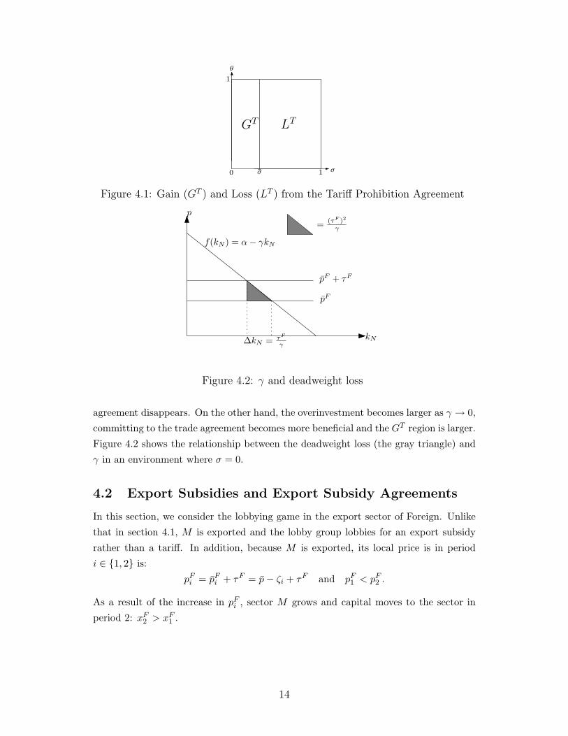
PROPOSITION 1 The government gains from the tariff prohibition agreement if

and only if σ < σ(γ).

When committing to the agreement, the overinvestment in period 1 is eliminated and

the government with a low bargaining power (σ < σ) gains from the agreement. A

similar result is found in Maggi and Rodriguiez-Clare (1998). Figure 4.1 depicts this

result. The horizontal and vertical axes show the values of σ and θ, respectively. The

GT and LT regions are the regions in which the government gains and loses from the

agreement, respectively.

Note that σ ∈ (0, 1), σ(γ) is increasing in γ (the slope of the demand for capital in

the numeriare sector), limγ→0+

σ(γ) = 1, and limγ→∞

σ(γ) = 0.11 The intuition is as follows.

From (4.10) and (4.15), we have:

f(k−xH1 )−f(k−xH

1 ) = τH(xH1 )−cH(xH

1 ) ⇒ xH1 −xH

1 =τ(xH

1 )− cH(xH1 )

γ=

1− σ

2γaxH

1 .

As γ → ∞, the overinvestment (xH1 − xH

1 ) approaches zero and the benefit from the

11Note that σ′(γ) = 2 − 2γ+1√γ2+γ

= 2 − 2γ+1√(γ+ 1

2 )2− 14

> 0 for γ > 0. From√

γ2 + γ − γ = γ√γ2+γ+γ

and

limγ→∞

γ√γ2+γ+γ

= 12 , we have lim

γ→∞σ(γ) = 0.

13

θ

1 σ0

1

GT

σ

LT

Figure 4.1: Gain (GT ) and Loss (LT ) from the Tariff Prohibition Agreement

pF

p

kN

f(kN ) = α− γkN

pF + τF

∆kN = τF

γ

= (τF )2

γ

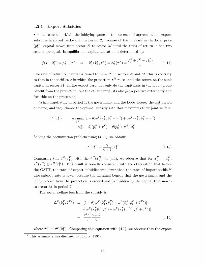
Figure 4.2: γ and deadweight loss

agreement disappears. On the other hand, the overinvestment becomes larger as γ → 0,

committing to the trade agreement becomes more beneficial and the GT region is larger.

Figure 4.2 shows the relationship between the deadweight loss (the gray triangle) and

γ in an environment where σ = 0.

4.2 Export Subsidies and Export Subsidy Agreements

In this section, we consider the lobbying game in the export sector of Foreign. Unlike

that in section 4.1, M is exported and the lobby group lobbies for an export subsidy

rather than a tariff. In addition, because M is exported, its local price is in period

i ∈ 1, 2 is:

pFi = pF

i + τF = p− ζi + τF and pF1 < pF

2 .

As a result of the increase in pFi , sector M grows and capital moves to the sector in

period 2: xF2 > xF

1 .

14

4.2.1 Export Subsidies

Similar to section 4.1.1, the lobbying game in the absence of agreements on export

subsidies is solved backward. In period 2, because of the increase in the local price

(pFi ), capital moves from sector N to sector M until the rates of return in the two

sectors are equal. In equilibrium, capital allocation is determined by:

f(k − xF2 ) = pF

2 + τF ⇒ xF2 (xF

1 , τF ) = xF2 (τF ) =

pF2 + τF − f(k)

γ. (4.17)

The rate of return on capital is raised to pF2 + τF in sectors N and M ; this is contrary

to that in the tariff case in which the protection τH raises only the return on the sunk

capital in sector M . In the export case, not only do the capitalists in the lobby group

benefit from the protection, but the other capitalists also get a positive externality and

free ride on the protection.

When negotiating in period 1, the government and the lobby foresee the last period

outcome, and they choose the optimal subsidy rate that maximizes their joint welfare:

τF (xF1 ) = arg max

τF

(1− θ)ωF (xF1 , pF

1 + τF ) + θωF (xF2 , pF

2 + τF )

+ a[(1− θ)(pF1 + τF ) + θ(pF

2 + τF )]xF1

Solving the optimization problem using (4.17), we obtain:

τF (xF1 ) =

γ

γ + θaxF

1 . (4.18)

Comparing this τF (xF1 ) with the τH(xH

1 ) in (4.4), we observe that for xF1 = xH

1 ,

τF (xF1 ) ≤ τH(xH

1 ). This result is broadly consistent with the observation that before

the GATT, the rates of export subsidies was lower than the rates of import tariffs.12

The subsidy rate is lower because the marginal benefit that the government and the

lobby receive from the protection is eroded and free ridden by the capital that moves

to sector M in period 2.

The social welfare loss from the subsidy is:

∆F (xF1 , τF∗) ≡ (1− θ)[ωF (xF

1 , pF1 )− ωF (xF

1 , pF1 + τF∗)] +

θ[ωF (xF2 (0), pF

1 )− ωF (xF2 (τF∗), pF

2 + τF∗)]

=τF∗2

2γ + θ

γ(4.19)

where τF∗ ≡ τF (xF1 ). Comparing this equation with (4.7), we observe that the export

12This asymmetry was discussed by Rodrik (1995).

15

subsidy in Foreign generates more welfare loss than the tariff in Home with the same

level. Substituting (4.19) and (4.18) into (4.5), we have:

cF (xF1 ) =

γ

2(γ + θ)(1 + σ)axF

1 . (4.20)

The net benefit to the government from the protection is:

gF (xF1 ) ≡ (cF (xF

1 )− ∆F (xF1 , τF∗)

axF1

)xF1 =

γ

2(γ + θ)σaxF 2

1 . (4.21)

The total protection surplus to the two bargaining parties receive is:

gF (xF1 ;σ = 1) =

γ

2(γ + θ)axF 2

1 .

The higher the value of θ is, the faster the new capital moves to sector M in period 2

and erodes the protection surplus. The entrance of new capital amplifies the deadweight

loss through overinvestment in period 2. In period 0, capital is allocated such that the

rates of return in the two sectors are equal:

θf(k − xF1 ) + (1− θ)f

(k − xF

2 (τF∗))

= θpF1 + (1− θ)pF

2 + τF∗ − cF (xF1 ). (4.22)

The LHS and the RHS are the total (periods 1 and 2) returns on capital allocated in

sector N and sector M , respectively. Simplifying (4.22) by using (4.20) and (4.18), we

have:

f(k − xF1 ) = pF

1 + τF (xF1 )− cF (xF

1 )1− θ

= pF1 +

(1− 2θ − σ)2(1− θ)(γ + θ)

aγxF1 . (4.23)

Solving this equation by using (4.20) and (4.18), we have:

xF1 =

2(1− θ)(γ + θ)(pF1 − f(k))

γh(θ)> 0 (4.24)

where h(θ) = 2γ − a(1− σ) + 2θ(a + 1− γ − θ).13 Differentiating (4.24), we have:

dxF1

dθ= −2aJ(σ)(pF

1 − f(k))bh2(θ)

< 0 (4.25)

where J(σ) = σ(b + 2θ − 1) + b − 1 − 2θ(1 − θ).14 Intuitively, as θ increases, the free-

rider problem is more severe and the incentive to invest capital in sector M in period

13The function h is a bell-shaped quadratic function. For θ ∈ [0, 1], h(θ) ≥ min(h(0), h(1)). From h(0) =2γ − a(1− σ) > 0 and h(1) = a(1− σ) > 0, we have h(θ) > 0 for θ ∈ [0, 1].

14J(0) = (1− θ)2 + θ2 + b and J(1) = 2(b + θ2). The linearity of J , J(0) > 0 and J(1) > 0 imply J(σ) > 0for σ ∈ [0, 1].

16

1 decreases. From (4.21) and (4.25), we have:

dgF

dθ=

∂gF

∂θ+

∂gF

∂xF1

∂xF1

∂θ< 0;

The rent that the government receive from protection is decreasing in θ.

Now, the game is solved. The government welfare under this game is:

ΩF = (1− θ)ωF (xF1 , pF

1 + τF∗) + θωF (xF2 (τF∗), pF

2 + τF∗) + acF (xF1 )xF

1 . (4.26)

4.2.2 Export Subsidy Prohibition Agreements

Now suppose that the Foreign government commits to an export subsidy prohibition

agreement before the lobbying game begins. Under this agreement, there is no lobbying

and τF = 0. Because the transportation cost drops, the local price of M increases. In

period 2, capital moves from sector N to sector M . In equilibrium, the sunk capital

constraint (xF1 ≥ xF

2 ) is not binding. Therefore, capital in periods 1 and 2 is allocated

according to:

f(k − xF1 ) = pF

1 and f(k − xF2 ) = pF

2 . (4.27)

Solving these two equations, we obtain:

xF1 =

pF1 − f(k)

γand xF

2 =pF2 − f(k)

γ. (4.28)

Comparing (4.23) and (4.27), we have:

xF1 > xF

1 for 2θ +σ < 1, xF1 < xF

1 for 2θ +σ > 1 and xF1 = xF

1 otherwise. (4.29)

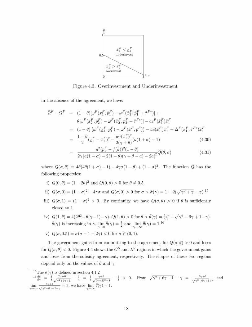
Figure 4.3 shows the overinvestment and underinvestment regions. In the northeast

region of figure 4.3, where θ and σ are high and 2θ + σ > 1, lobbying creates underin-

vestment in period 1. The rate of return from investing capital in sector M in period 1

is small because the lobby’s bargaining power (1−σ) is small. Moreover, high θ results

in a high incentive for capitalists to invest in sector N in period 1 and to wait to free

ride on the positive externality from the protection. These two effects together result

in underinvestment in period 1. On the other hand, in the southwest region of figure

4.3, the lobbying creates overinvestment in period 1.

Subtracting the government welfare under the subsidy agreement (ΩF ) from that

17

θ

1

0.5

σ0

1

xF1 < xF

1

xF1 > xF

1

underinvest

overinvest

Figure 4.3: Overinvestment and Underinvestment

in the absence of the agreement, we have:

ΩF − ΩF = (1− θ)[ωF (xF1 , pF

1 )− ωF (xF1 , pF

1 + τF∗)] +

θ[ωF (xF2 , pF

2 )− ωF (xF2 , pF

2 + τF∗)]− acF (xF1 )xF

1

= (1− θ)(ωF (xF

1 , pF1 )− ωF (xF

1 , pF1 )

)− ac(xF

1 )xF1 + ∆F (xF

1 , τF∗)xF1

=1− θ

2(xF

1 − xF1 )2 − aγ(xF

1 )2

2(γ + θ)(a(1 + σ)− 1) (4.30)

=a2(pF

1 − f(k))2(1− θ)2γ [a(1− σ)− 2(1− θ)(γ + θ − a)− 2a]2

Q(θ, σ) (4.31)

where Q(σ, θ) ≡ 4θ(4θ(1 + σ)− 1)− 4γσ(1− θ) + (1− σ)2. The function Q has the

following properties:

i) Q(0, θ) = (1− 2θ)2 and Q(0, θ) > 0 for θ 6= 0.5.

ii) Q(σ, 0) = (1− σ)2 − 4γσ and Q(σ, 0) > 0 for σ > σ(γ) = 1− 2(√

γ2 + γ − γ).15

iii) Q(σ, 1) = (1 + σ)2 > 0. By continuity, we have Q(σ, θ) > 0 if θ is sufficiently

closed to 1.

iv) Q(1, θ) = 4(2θ2+θ(γ−1)−γ). Q(1, θ) > 0 for θ > θ(γ) = 14(1+

√γ2 + 6γ + 1−γ).

θ(γ) is increasing in γ, limγ→0

θ(γ) = 12 and lim

γ→∞θ(γ) = 1.16

v) Q(σ, 0.5) = σ(σ − 1− 2γ) < 0 for σ ∈ (0, 1).

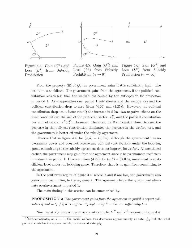
The government gains from committing to the agreement for Q(σ, θ) > 0 and loses

for Q(σ, θ) < 0. Figure 4.4 shows the GS and LS regions in which the government gains

and loses from the subsidy agreement, respectively. The shapes of these two regions

depend only on the values of θ and γ.

15The σ(γ) is defined in section 4.1.216 dθ

dγ = 18

2γ+6√γ2+6γ+1

− 14 = 1

4γ+3√

(γ+3)2−8− 1

4 > 0. From√

γ2 + 6γ + 1 − γ = 6γ+1√γ2+6γ+1+γ

and

limγ→∞

6γ+1√γ2+6γ+1+γ

= 3, we have limγ→∞

θ(γ) = 1.

18

θ

1

0.5

σ0

GS

LS

GS

1

θ

σ

Figure 4.4: Gain (GS) andLoss (LS) from SubsidyProhibition

θ

σ

0.5

σ0

LS

1

GS

GS

θ

Figure 4.5: Gain (GS) andLoss (LS) from SubsidyProhibition (γ → 0)

θ

1

0.5

σσ

1 θ

LS

Figure 4.6: Gain (GS) andLoss (LS) from SubsidyProhibition (γ →∞)

From the property (ii) of Q, the government gains if θ is sufficiently high. The

intuition is as follows. The government gains from the agreement, if the political con-

tribution loss is less than the welfare loss caused by the anticipation for protection

in period 1. As θ approaches one, period 1 gets shorter and the welfare loss and the

political contribution drop to zero (from (4.20) and (4.25)). However, the political

contribution drops at a faster rate17; the increase in θ has two negative effects on the

total contribution: the size of the protected sector, xF1 , and the political contribution

per unit of capital, cF (xF1 ), decrease. Therefore, for θ sufficiently closed to one, the

decrease in the political contribution dominates the decrease in the welfare loss, and

the government is better off under the subsidy agreement.

Observe that in figure 4.4, for (σ, θ) = (0, 0.5), although the government has no

bargaining power and does not receive any political contributions under the lobbying

game, committing to the subsidy agreement does not improve its welfare. As mentioned

earlier, the government may gain from the agreement since it helps eliminate inefficient

investment in period 1. However, from (4.29), for (σ, θ) = (0, 0.5), investment is at its

efficient level under the lobbying game. Therefore, there is no gain from committing to

the agreement.

In the southwest region of figure 4.4, where σ and θ are low, the government also

gains from committing to the agreement. The agreement helps the government elimi-

nate overinvestment in period 1.

The main finding in this section can be summarized by:

PROPOSITION 2 The government gains from the agreement to prohibit export sub-

sidies if and only if i) θ is sufficiently high or ii) θ and σ are sufficiently low.

Now, we study the comparative statistics of the GF and LF regions in figure 4.4.

17Mathematically, as θ → 1, the social welfare loss decreases approximately at rate 12−θ but the total

political contribution approximately decreases at rate 11−θ

19

θ

1

0.5

σ0

1

θ

LT , GSGT , LS

GT , LS

GT , GS

LT , GS

σ

Figure 4.7: Gain and Loss from Subsidy Prohibition and Tariff Prohibition

Because the function Q has only one parameter (γ), the shapes of the GF and LF

regions depend only on γ. To study how these regions change as γ changes, we consider

the two extreme cases: γ → 0 and γ →∞. Figures 4.5 shows the GF and LF regions,

generated numerically for γ → 0. Comparing figure 4.4 with figure 4.5, we see that the

LF region shrinks and the GF region grows as γ drops to zero. The term γ is the slope

of the demand for capital in the each numeriare sector; it is positively related to the

elasticity of the demand for capital in this sector. The higher the value of γ is, the more

responsive is the demand for capital to the change in the rate of return in the numeriare

sector. As discussed in section 4.1.2, for γ → 0, investment is highly responsive to the

protection. The overinvestment or underinvestment in period 1 caused by lobbying is

high and the agreement brings more benefit to the government. Therefore, the GF

region gets larger as γ → 0. On the other hand, in figure 4.6, for γ →∞, investment in

period 1 is irresponsive to protection, the agreement has no benefit to the government

and the GF region disappears.

4.3 Optimal Agreements

In this section, we suppose that Home and Foreign are under an international trade

agreement on tariffs and subsidies. We find the condition in which it is optimal for the

agreement to ban export subsidies but allow import tariffs.

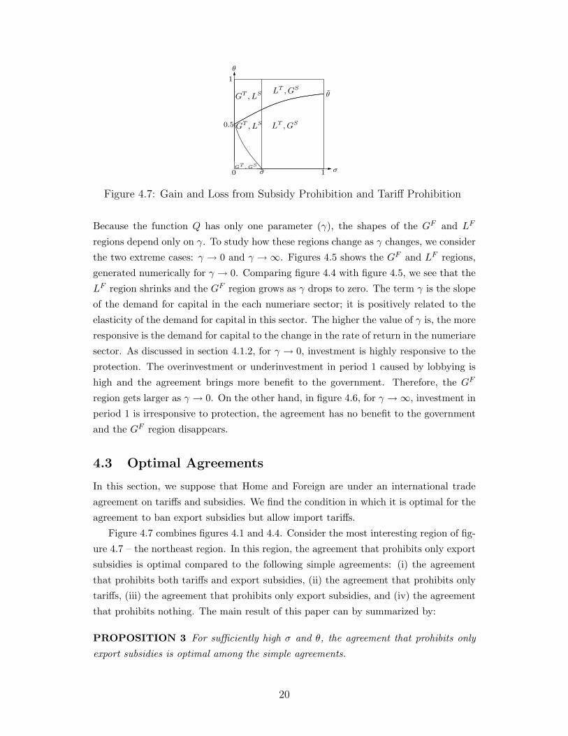
Figure 4.7 combines figures 4.1 and 4.4. Consider the most interesting region of fig-

ure 4.7 – the northeast region. In this region, the agreement that prohibits only export

subsidies is optimal compared to the following simple agreements: (i) the agreement

that prohibits both tariffs and export subsidies, (ii) the agreement that prohibits only

tariffs, (iii) the agreement that prohibits only export subsidies, and (iv) the agreement

that prohibits nothing. The main result of this paper can by summarized by:

PROPOSITION 3 For sufficiently high σ and θ, the agreement that prohibits only

export subsidies is optimal among the simple agreements.

20

As mentioned above, whether the Home government gains or loses from an agree-

ment to prohibit tariffs depends only on its bargaining power (σ). With a sufficiently

high bargaining power, the Home government receives large political contributions from

using tariffs and an agreement to prohibit tariffs is not desirable. On the other hand,

whether an agreement to prohibit export subsidies is desirable to the Foreign govern-

ment or not depends on σ and θ. For a sufficiently high θ, the political contribution

that the Foreign government receives from export subsidies are highly eroded by free

riders and the government would be better off when committing to prohibit export

subsidies. Therefore, for sufficiently high σ and θ, the optimal agreement is the one

that prohibits only export subsidies.

5 Conclusion

In this paper, we proposed a simple small-country model to explain the asymmetric

treatment between import tariffs and export subsidies in the WTO. In our model, the

anticipation for protection creates inefficient investment. A government may choose to

commit to a tariff prohibition agreement and/or export subsidy prohibition agreement

to eliminate this anticipation and to have a social welfare gain. However, when com-

mitting to these agreements, the government loses the political contributions collected

from protection. Therefore, the government commits to a trade agreement, if the social

welfare gain is greater than the loss in political contributions.

In an environment where transportation costs are decreasing, export sectors grow

and import-competing sectors decline. In export sectors, export subsidies attract new

entrants and investment. These entrants erode the protection rent. The rent that the

government can get from protecting these sectors is, therefore, small. On the other

hand, import-competing sectors decline. In these sectors, the return on capital drops.

Capital is sunk and cannot move out. This sunk capital allows protection to raise the

rate of return in these sectors without attracting entry as long as the rate of return on

the sunk capital is lower than the normal rate of return. The protection rent in import-

competing sectors is not eroded by new entrants and the government may extract large

political rent. In this environment, we find that under the condition in which the

government has a high bargaining power and capital moves fast, the optimal agreement

prohibits only export subsidies and allows the use of tariffs.

21

6 References

Bagwell, K. and Staiger, R. W. (1999): “An Economic Theory of GATT,” American EconomicReview, 89, 215-48.

Bagwell, K. and Staiger, R. W. (2001): “Strategic Trade, Competitive Industries and Agri-cultural Trade Disputes, Economics and Politics, 113-128.

Baldwin, J.R. and Gu, W. (2004): “Trade Liberalization: Export-market Participation, Pro-ductivity Growth and Innovation,” Oxford Review of Economic Policy, 20, 372-392.

Baldwin, R. and Robert-Nicoud, F. (2002): “Entry and Asymmetric Lobbying: Why Gov-ernments Pick Losers,” NBER working paper no. 8756.

Bernard, A.B. and Jensen, J.B. (2002): “The Deaths of Manufacturing Plants,” NBER workingpaper no. 9026

Brander, J. A. and Spencer, J. B. “Export Subsidies and International Market Share Rivalry,”Journal of International Economics, 18(2), 83-100.

Ethier, W. J. (2003): “Trade Agreements Based on Political Externalities,” mimeo, Univer-sity of Pennsylvania.

Feenstra, R.C, Romalis, J. and Schott, P.K. (2002): “U.S. Imports, Exports and Tariff Data,”NBER Working Paper No. 9387.

Glismann, H. and F. Weiss (1980): “On the political economy of protection in Germany,”World Bank Staff WP 427.

Grossman, G. and E. Helpman (1994): “Protection for Sale,” American Economic Review,84(4), 833-850.

Grossman, G. and E. Helpman (1995): “Trade Wars and Trade Talks,” Journal of PoliticalEconomy, 103(4), 675-708.

Grossman, G. and E. Helpman (1996): “Rent Dissipation, Free Riding, and Trade Policy,”European Economic Review, 40, 795-803.

Hufbauer, G. and H. Rosen (1986): Trade Policy for Troubled Industries, Policy Analyses inInternational Economics 15, Institute for International Economics Washington, D.C.

Hufbauer, G., D. Berliner and K. Elliot (1986): Trade Protection in the United States: 31Case Studies, Institute for International Economics, Washington, D.C.

Johnson, H. (1954): “Optimum Tariffs and Retaliation,” Review of Economic Studies 21(2),142- 153.

Levy, I. P. (1999): “Lobbying and International Cooperation in Tariff Setting,” Journal ofInternational Economics, 47, 345-70.

Maggi, G. and Rodriguez-Clare, A. (1998): “The Value of Trade Agreements in the Pres-ence of Political Pressures,” Journal of Political Economy, 106, 574-601.

22

Maggi, G. and Rodriguez-Clare, A. (2005a): “A Political-Economy Theory of Trade Agree-ments,” mimeo, Princeton University.

Maggi, G. and Rodriguez-Clare, A. (2005b): “Import Tariffs, Export Subsidies and the Theoryof Trade Agreements,” mimeo, Princeton University.

Mitra, D. (2002): “Endogenous Political Organization and the Value of Trade Agreements,”Journal Of International Economics, 57, 473-485.

Rodrik, D. (1995), “Political Economy of Trade Policy,” In: Grossman, G. and K. Rogoff[eds.], Handbook of International Economics (Amsterdam: North-Holland), 1457-1495.

Staiger, R.W., and Tabellini, G. (1987) “Discretionary Trade Policy and Excessive Protec-tion,” American Economic Review, 77, 823-37.

Subramanian, A. and Wei, S.J. (2003): “The WTO Promotes Trade, Strongly But Unevenly,”NBER Working Paper No. 10024. U.S.

Tornell, A. (1991): “Time Inconsistency of Protectionist Programs,” Quarterly Journal of Eco-nomics 106, 963-74.

23