Inefficient Policies, Inefficient Institutions and Trade∗

Ruben Segura-Cayuela

MIT

July 2006

Abstract

Despite the general belief among economists on the growth-enhancing role of in-

ternational trade and significant trade opening over the past 25 years, the growth

performance of many developing economies, especially of those in Latin America and

Africa, has been disappointing. While this poor growth performance has many po-

tential causes, in this paper I argue that part of the reason may be related to the

interaction between weak institutions and trade. In particular, I construct a model in

which trade opening in societies with weak institutions (in particular autocratic and

elite-controlled political systems) may lead to worse economic policies. The reason is

that general equilibrium price effects of taxation and expropriation in closed economies

also hurt the elites, and this puts a natural barrier against inefficient policies. Trade

openness removes this barrier and enables groups with political power to exercise this

power in more inefficient ways.

∗I am indebted to Daron Acemoglu, Pol Antras, Guido Lorenzoni and Jaume Ventura for invaluableguidance, to Raphael Auer, Karna Basu, Veronica Rappoport and Tal Regev for very helpful comments andto Francesco Giavazzi for very helpful comments and for allowing me to use his data. I have also benefitedfrom suggestions by participants at the MIT Macroeconomics Lunch and the MIT International Seminar.Financial support from the Bank of Spain is gratefully acknwoledged. All remaining errors are my own.Email: rubens@mit.edu

1

1 Introduction

Increasing globalization has been a defining feature of the postwar era. There is some

consensus that this has been beneficial for economic performance: trade brings about a more

efficient allocation of resources through technology or factor endowment driven comparative

advantage, or through better exploitation of increasing returns to scale. Figure 1 gives a

sense of this. Countries that traded more between 1960 and 1995 appear to have larger per

capita incomes today.1

At the same time, some less-developed economies have seen little improvement in eco-

nomic performance since the 1960’s. Figure 2 splits Figure 1 in two. On the top are countries

that, from 1960 to 2000, had on average limited or no constraints on executive power (non-

democratic regimes). The bottom section shows countries with strong checks on the executive

power over the same period (more democratic regimes). A positive correlation between trade

and income holds for more democratic countries, but for less democratic regimes there is no

positive correlation. It could be argued that this is unrelated to globalization, or that these

countries have not opened to trade enough to benefit from it. However, trade as a share

of GDP in those countries has increased from an average of 33% in 1960, to an average of

almost 60% in 2000.2 Although most trade takes place between developed nations, it is still

true that less-developed economies today trade much more than they did 40 years ago.

The alternative view developed in this paper is that our standard trade models are missing

an important ingredient. If we are to look for a fundamental difference between countries in

the North and countries in the South that might affect trade predictions, institutions stand

out as a clear candidate. How do institutions in the North differ from those in the South? The

answer is straightforward: institutions in the South tend to be less efficient, their economies

are characterized by corruption, expropriation, or weak property rights protection.

Do countries with inefficient institutions, then, benefit from trade in the way our stan-

dard models would predict? Trade theories typically formalize differences in institutions as

differences in exogenous parameters or differences in productivity. But institutions in the

South are inefficient in a distortive way: groups with political power tend to extract rents

from other groups in society, which affects the incentives in these economies. Such ineffi-

ciencies can alter standard trade predictions in two ways. First, they can have distributive

consequences: winners and losers from the process of trade integration may differ from those

predicted by standard theories.3 Second, trade might affect the inefficiency of institutions

1We are aware of the standard omitted variable and reverse causality problems. We are just describingcorrelations.

2The measure we are using is exports plus imports as a share of GDP from the Penn World Tables.3Levchenko (2004) is an example of this.

2

itself. Exogenous differences in productivity parameters are not likely to capture the effects

of institutional variance.

The main contribution of this paper is to answer this question, endogenizing the efficiency

of institutions and analyzing how this efficiency changes when economies open to interna-

tional trade. I argue that part of the reason why less-developed economies may not have

benefited from international trade is that, in countries with weak or non-democratic political

institutions, trade liberalization may lead to worse policies and economic institutions. The

reasoning is simple: in a closed economy, groups that hold political power are restrained

in the degree to which they may indulge inefficient redistributive policies, such as corrup-

tion or expropriation, because of the general equilibrium price effects such policies create.

Increased international trade removes these price effects, and may increase the intensity of

rent-extracting policies to the point where it more than outweighs for standard trade gains.

In such situations, trade may not be welfare enhancing.

To examine this issue, I build on Acemoglu (2005), which provides a framework to help

understand why inefficient institutions emerge. The starting point of my paper is a society

that already has an elite with a preference for inefficient policies in place. In particular,

I start with a set of political institutions that give all political power to an elite minority.

This power allows the elite to benefit from its policies regardless of how they affect the rest

of society. Throughout this paper, this state is the definition of the term “dictatorship.”

The key policies in this model are group specific tax rates, which are distortionary. In this

model there are no other means to extract resources from non-elite groups. The definition

of taxation in this discussion is broad: it is any policy that leads to investment distortions

in the economy (such as expropriation or corruption).

I focus on two sources of inefficiency in policies, both arising from the desire and ability

of the elite to extract resources from other groups. First, the elite might set distortionary

taxes to extract revenue from other groups. We refer to this as Revenue Extraction. Second,

because they participate in production activities, the elite producers can also benefit through

an indirect channel. By taxing other groups with production activities, they reduce the

demand for factors of these groups. This benefits them through lower factor prices and

higher profits. We refer to this second source of inefficiency as Factor Price Manipulation.

The degree of expropriation in the economy and its effect will depend on the strength of

these two sources of inefficiencies.

I first analyze the closed economy. In Acemoglu (2005), elite and non-elite producers

compete in the same sector; i.e., products of both groups are perfect substitutes.4 I depart

from that assumption by allowing elite and non-elite producers to produce in different sectors

4Additionally, Acemoglu (2005) only analyzes a closed economy.

3

and assuming that these sectors have certain complementarity. This immediately implies a

natural restriction on the extent to which the elite can either extract resources from the

middle class or modify factor prices. Any taxes the elite place on the middle class will come

back to affect them. Higher taxes will imply a higher cost for the consumption bundle,

which will reduce the real value of the elites’ income. And this is true for both sources

of inefficiency, Revenue Extraction and Factor Price Manipulation. Taxing these non-elite

groups will not only directly reduce non-elite producers investment (the standard Laffer

Curve effect) but also, because goods produced by these non-elite producers will become

more expensive, reduce the value of the elite’s profits. In other words, as long as the elite

consumes what non-elite groups produce, the elite will find expropriation and excessive

taxation less desirable because these policies will make consumption more expensive.

The key assumption in this analysis is that elite producers care, not only about tax

revenues, but also about profits. This encourages them to tax both sectors asymmetrically,

since taxing themselves hurts profits. But taxing sectors differently distorts the relative price

and allocation of resources in the economy. And this also reduces profits through the general

equilibrium: a tax on the middle class decreases the relative price of the goods produced by

the elite, which decreases profits. This is what limits the elite from taxing other groups as

much as they would like.

Opening the economy to trade will increase competition, which will increase the substi-

tutability between goods produced by elite and non-elite producers. In other words, trade

will reduce the negative general equilibrium effect (on the elites’ income) of taxing these

other groups; now, the elite can find most goods in world markets. This frees the elite to

take full advantage of their policy control, translating into greater inefficiency as taxes rise

aggressively on all other groups. The welfare implications of opening to trade will depend

on whether the increase in expropriation more than outweighs for the standard gains from

trade. The most important result of this paper is its assertion that, in dictatorial states,

international trade is not necessarily welfare improving for the whole economy.

I then repeat the analysis for a democracy, which we define as political institutions that

give all political power to the majority. A democracy with a closed economy will be inefficient

to some extent, although generally less inefficient than a dictatorship. The surprising result

is that once we open to trade, policies do not necessarily become more efficient; instead, they

remain constant. A look at the nature of our democratic model explains this. A democracy

gives the political power to the majority, and in our model that majority is comprised of

workers. Since workers participate in both sectors of the economy, they will try not to distort

resource allocation across sectors. Also, workers care about wages (not profits), which implies

that the general equilibrium effect will not restrain them from achieving their desired tax

4

rates. When the country opens to trade, workers will set the same tax rates as in the closed

economy, and opening to trade will not have a negative effect on the efficiency of policies.

Trade is always welfare enhancing under a democracy.

The main contribution of this paper is to emphasize the negative impact that trade has

on expropriation and income of countries with weak political institutions, by making non-

elite and elite sectors more substitutable. The literature has emphasized how globalization,

by allowing capital mobility, leads to lower taxation. I abstract from this mechanism by

assuming that there is no international factor mobility.5 The paper most closely related to

this one, in spirit, is Bourguignon and Verdier (2000).6 In their model, an oligarchy of capi-

talists, operating in an economy with missing financial markets for the financing of human

and physical capital investments, might find it in their interest to subsidize the education

of the poor because both types of capital are complementary. Political participation in this

model is linked to education, which means that the elite are willing to subsidize education

despite the cost in terms of political power. With international financial integration, the

return on investments of the capitalist is given by the international rate of interest, which

breaks the complementarity between human capital and capital accumulation. The elite may

stop subsidizing the education of the poor, which implies a reinforcement of their political

power.7 Notice the differences between their approach and mine. Their paper looks at how,

for a given degree of inefficiency, political institutions change with trade.8 My paper instead

takes institutions as given and analyzes the change in their inefficiency. Also their paper is

about whether trade delays or not democratization, not about the effects on Welfare.9

This paper is of course related to Segura-Cayuela (2006a), which shows empirical evidence

on the relevance of the forces at play in the current paper.10 This paper is also related to

Epifani and Gancia (2005), who analyze the size of governments in the context of benevolent

rulers that provide a public good. Because trade shifts part of the tax burden away, trade

integration in such situations leads to higher taxation and bigger government. But the

mechanics of their model are very different to mine. First, there is no distinction between

5It is not obvious how this might affect the results of the paper. To add this mechanism, we would haveto think carefully about who owns the capital in the economy. It seems safe to assume, for present purposes,that in underdeveloped economies capital is in the elite’s hands.

6In Bourguignon and Verdier (2005), the authors make a similar argument in the context of trade inte-gration and factor mobility.

7Verdier (2005) provides a good discussion on how trade might affect domestic policy.8By inefficiency in their model I mean the lack of financial markets.9Of course democratization can have effects on Welfare. But there is no explicit discussion of the con-

sequences in the context of their model. In their model, liberalizing financial markets slows human capitalaccumulation, but increases physical capital accumulation.10In that paper I show evidence that expropriation increases with trade opening for non-democratic coun-

tries, while it is reduced for democratic ones, consistent with the main theoretical prediction of this paper.

5

good/bad political institution. Their analysis is about benevolent governments providing

public goods. Also, taxation at home increases because foreigners pay some of it, through

prices of imports. In my model taxation increases irrespective of who exports or imports.

All it matters is that goods produced by the middle class can be found somewhere else.

Finally, this paper is related also to the recent literature on the effect of trade in institutions,

Levchenko (2004), Segura Cayuela (2006b), Do and Levchenko (2005), and chapter 10 on

Acemoglu and Robinson (2005), among others.11

The rest of the paper is organized as follows. Section 2 presents the basic economic

model and characterizes the economic and political equilibrium in a closed economy under a

dictatorship of the elite. Section 3 repeats the exercises in Section 2, but for an open economy.

Section 4 analyzes the welfare implications of opening to trade. Section 5 discusses how the

analysis changes under a democracy. Finally Section 6 concludes.

2 The General Model with a Closed Economy

This section develops the basic economic model in a closed economy, where inefficiencies

will arise due to limited checks on the executive power and the desire of the minority elite

to extract rents from other groups in society. I will first solve for the economic equilibrium

for a given set of policies, and then I will characterize the political equilibrium. I start by

describing the general environment.

2.1 Environment

Consider an economy, closed to international trade for the time being, populated by a

continuum of agents 1+θe+θm that consume a single final good, y. Preferences of the agents

are defined as

U = y.

The final good is produced by combining two intermediate inputs, ye and ym, according to

technology

y = β−β(1− β)−(1−β) (ye)β (ym)1−β , (1)

where I define χ ≡ β−β(1 − β)−(1−β). There are three groups of agents. First, a mass 1

of workers, endowed with 1 unit of labor each, which they supply inelastically. Second, the

middle class producers, denoted by m, who have access to production opportunities in sector

11For the effects of institutions in trade/FDI, see for instance Levchenko(2004), Antras (2003, 2005), orAntras and Helpman (2005).

6

m. Finally, the elite producers, e, who also have access to production opportunities in sector

e and hold the political power.12

Technology is identical in both sectors,

yji =1

1− α

¡kji¢1−α ¡

lji¢α

, (2)

where yji stands for production of individual i of group j, k denotes capital and l labor.

Capital is assumed to fully depreciate after use.13 In what follows, total variables for a

group will simply be the value of that variable for an individual of that group, times the size

of that group, j, θj .

The political power in this model will be in the hands of the elite.14 They have the ability

to decide policies and choose those that benefit them the most. The only policies in this

model consist of the ability to tax the activity of both intermediate sectors with a rate τ j.

Again, we should interpret the concept of taxation in a broader sense: it could correspond

to expropriation, or corruption, or any policy used by the elite to repress the middle class

that translates into distortions in the economy.

Let us assume the following timing of events: first, taxes are set, then, investments are

made. This way, we can abstract from inefficiencies due to hold-up problems, which could

be interesting to analyze but are not the scope of this paper. Revenue from taxation can

be distributed across groups with targeted lump-sum transfers towards each group, T j ≥ 0.The government budget constraint is

Tw + θmTm + θeT e ≤ φ

Zj,i

τ jpjyji didj, (3)

where pj denotes the price of good j and φ is a parameter that measures the ability of the

elite to collect and redistribute taxes, state capacity. In less-developed economies, fiscal

systems are typically inefficient; this is due to large informal economies or corruption in the

collection of taxes, for instance. So it should be natural to think that φ < 1 for this type of

economy: what the government redistributes is less than what it collects. For most of the

analysis in this paper I will assume that this is the case, although I will discuss the results

for φ = 1 too. Notice that there are no other fiscal instruments, only distortionary taxes,

12Most of the analysis in this paper would stand if I allowed both groups to produce in both sectorswith different productivities. The assumption that they each perform in one of the sectors simplifies thediscussion.13A discussion of this assumption is found in Segura Cayuela (2006b).14I assume that the elite producers hold the political power until I analyze the model in the context of a

democracy. But for the analysis in this section, the economic equilibrium, who holds the political power willbe irrelevant.

7

which will be the root for the inefficiency of policies.

There is a maximum scale, lj ≤ λ, for each firm. And each member of a group can just

set up one firm. The role of this assumption is to generate profits in equilibrium: if a group

of producers reach their maximum scale, they will make profits. Notice that if

λθe + λθm < 1, (4)

there is going to be excess labor supply in this economy, the total amount of labor that both

groups demand is smaller than the supply of labor, 1. When Condition (4) holds, the wage

rate will drop to 0. When it does not hold, we have excess demand for labor, which will give

us a positive wage rate in equilibrium. Thus we can write labor market clearing as

θmlmi + θelei ≤ 1, (5)

where lji will be the labor demand of an individual i of group j, and (5) is satisfied with

equality when Condition (4) does not hold. Throughout the paper we analyze the results

both when Condition (4) holds and when it does not, because that will allow me to separate

the two sources of inefficiency.15

2.2 Economic Equilibrium in the Closed Economy

An economic equilibrium is a set of intermediate and final good prices, p, pe, pm, wage

w, investment levels and employment levels for all producers {kj, lj}j=e,m, such that givena set of taxes, τ e, τm, and p, pe, pm, w, all producers choose investment and employment

optimally, good markets clear, and labor market clears.

The problem for the final good producers is given by,

Minye,ym

peye + pmym s.t.

y ≤ χ (ye)β (ym)1−β .

This minimization yieldsye

ym=

β

1− β

pm

pe, (6)

Let us normalize p = (pe)β (pm)1−β = 1. Intermediate goods producers maximize profits

taking the price and wage rate as given, which can be written as

15This will become clearer when we analyze the political equilibrium.

8

max(1− τ j)

1− αpj¡kji¢1−α ¡

lji¢α − wlji − kji , (7)

where j = e,m. As there is no initial or final stock of capital, we are basically assuming that

intermediate goods producers in each sector use units of final output to produce their goods.

This implies that the price of capital is one, as it can be seen in (7). This problem yields

kji =¡pj¡1− τ j

¢¢ 1α lji (8)

lji =

⎧⎪⎨⎪⎩= 0 if w > α

1−α ((1− τ j)pj)1/α

∈ [0, λ] if w = α1−α ((1− τ j)pj)

1/α

= λ if w < α1−α ((1− τ j)pj)

1/α

(9)

Notice first in (9) that, whenever the marginal product of labor is smaller than the wage,

the producer does not hire any workers. When the marginal product is bigger than the wage

rate, a producer i of group j hires labor until reaching the maximum scale λ. It is also

worth discussing the source of inefficiency in this economy. Looking at (8) we see that taxes

discourage investment. This is because producers are only able to recover a fraction of what

they invest.

We can replace (8) in (2) to find output for each individual of a group as a function of

their labor demand,

yji =1

1− α

¡pj¡1− τ j

¢¢ 1−αα lji (10)

and, using (10) together with (8) , we can solve for the profits of each individual as a function

of the price of that sector and the wage rate,

πji =

µα

1− α

¡pj¡1− τ j

¢¢ 1α − w

¶lji . (11)

For a given wage rate and employment, both output and profits will decrease with taxation

because investment decreases. It will be useful to combine (10) with (6) to solve for the

relative price of the two sectors (where recall that yj = θjyji ),

pe

pm=

µ1− τm

1− τ e

¶1−αµβ

(1− β)

θmlmiθelei

¶α

. (12)

Most of the economic equilibrium has been already characterized. Because the impli-

cations for prices and wages of the model will differ, depending on whether there is full

employment or not, we will analyze these two cases separately in the next subsections. I first

analyze the equilibrium with excess labor supply and, in this case in which the wage rate

drops to 0, firms will always make positive profits. When I analyze the equilibrium when

9

the labor market clears we will describe two types of equilibria. First, one in which nobody

makes profits because they do not reach the capacity constraint, and second, one in which

one of the groups reaches the capacity constraint and makes profits. Who makes the profits,

and when, will be a crucial question for the characterization of the political equilibrium.

2.2.1 The Economic Equilibrium with Excess Labor Supply

When Condition (4) holds, there is excess supply of labor in equilibrium and w = 0.

Equation (11) reveals that producers in both sectors always have positive profits, leading

them to hire the maximum amount of labor possible: le = λθe and lm = λθm. It is clear

then that taxes do not affect relative labor demands by each group. This is the main

difference with the full employment case, and we will discuss the role it plays for the political

equilibrium in the following sections.

With relative labor demands constant, the only way taxes affect output and profits is

through investment and prices. Once we take into account the equilibrium levels of employ-

ment, (12) translates into

pe

pm=

µ1− τm

1− τ e

¶1−αµβ

(1− β)

λθm

λθe

¶α

.

The interpretation of this relative price equation is straightforward. For given tax rates,

when the ratio of the middle class’ size relative to the size of the sector in which they produce,

λθm/(1−β), is larger than the same ratio for the elite, the relative price of the good producedby the elite increases. For given relative sizes, increased tax rates in the middle class sector

lead to smaller investment, which translates into lower production and a higher relative price

for that good.

We can combine (12) with the price normalization to solve for the price levels as

pe =

µ1− τm

1− τ e

¶(1−β)(1−α)µβ

(1− β)

λθm

λθe

¶(1−β)α(13)

pm =

µ1− τm

1− τ e

¶−β(1−α)µβ

(1− β)

λθm

λθe

¶−βα. (14)

The next proposition summarizes the economic equilibrium when there is excess supply

(proof in text):

Proposition 1 When Condition (4) holds, for given taxes τ e and τm, the economic equilib-

rium takes the following form: there is excess supply of labor, w = 0, and prices are given

10

by (13) and (14) . Given prices and wage rates, investment, employment, and output in each

sector are given by (8) , (9) and (10) , respectively.

It is useful to derive profits for each group and total output in the economy for future

reference. Replace (13) and (14) in (10) , and then replace the resulting equation in (1) to

find total output in the economy as

y =χ (λθe)β (λθm)1−β

1− α

¡(1− τ e)β(1− τm)(1−β)

¢(1−α)/α. (15)

Again, it is clear that taxation in each sector reduces investment in that sector, which

translates into a reduction of total output. Profits for each group are derived by replacing

(13) and (14) into (11) , and taking into account that all producers reach the maximum scale,

πe =α (λθe)β (λθm)1−β

1− α

µβ

1− β

¶(1−β)(1− τ e)

1/α

µ(1− τm)

(1− τ e)

¶(1−β)(1−α)/α(16)

πm =α (λθe)β (λθm)1−β

1− α

µβ

1− β

¶−β µ(1− τ e)

(1− τm)

¶β(1−α)/α(1− τm)1/α. (17)

A number of points are worth mentioning. First, because the wage rate drops to 0, both

groups make profits. Second, as mentioned before, taxing a sector reduces profits of the

producers in that sector. Finally, for any of the groups, a tax in the other group’s sector

reduces their profits through its effect on the price. Taxing sector m makes the unit price of

the consumption good more expensive, which decreases the real value of profits for the elite.

As we have normalized the unit price to 1, this increase in the unit price translates into the

price of sector e going down.

2.2.2 The Economic Equilibrium with Labor Market Clearing

The main difference in the case discussed in this section is that, as the labor market

clears, differential tax rates across various sectors will affect the relative demand for labor

in those sectors. To make profits, producers need to reach their maximum scale. Thus,

the group that controls taxation -in this section the elite- can use taxes to modify relative

demands and make profits in equilibrium. The more they turn relative demand in their

favor, the less labor the other groups demand, which translates into lower factor prices and

higher profits for the elite.

When Condition (4) does not hold, we can have two types of equilibria: one in which

demand for goods produced by each group never exceeds what they can produce, and another

11

in which one group reaches the maximum scale.16 The type of equilibrium we have will

depend, for given taxes, on the size of both groups. It will be important to understand when

any of the groups reach their maximum scale, because that is what determines profits and

what will determine taxation once we analyze the political equilibrium. For this reason, we

first characterize the equilibrium when none of the producers reach the maximum scale.

In this case, given that producers are price-takers, they make no profits in equilibrium,

which looking at (11) pins down price levels,

pj = wα

µ1− α

α

¶α1

(1− τ j), (18)

and using this together with the price normalization we get the following expression for the

wage rate,

w =α

1− α

¡(1− τ e)β(1− τm)(1−β)

¢1/α. (19)

From (19) we see that the wage rate will depend on both tax rates. When the labor market

clears, because both sectors are not perfect substitutes for each other, labor demands for

each sector will depend on tax rates, and this feeds back into the wage rate. We can now

combine the relative price equation (12) with the price levels (18) and the wage rate (19) to

derive the equilibrium levels of employment in each sector, lj = θjlji ,

le =1

1 + (1−β)(1−τm)β(1−τe)

, lm =1

1 + β(1−τe)(1−β)(1−τm)

. (20)

We can see from (20) how taxes distort the relative allocation of resources between sectors.

An increase in τ e increases the relative price of good e, which decreases the relative demand

for that good. In equilibrium, less labor will be allocated to that sector (and consequently

less investment, as investment is proportional to labor), and more to sector m.

The equilibrium just derived holds as long as none of the groups reach their capacity

constraint on labor. In particular, for this to be an equilibrium we need the equilibrium

levels of employment to be smaller than the maximum scale for each group, le ≤ λθe and

lm ≤ λθm. Combining these conditions with (20) we can express them as

1− τm

1− τ e≥ β

1− β

1− λθe

λθe≡ σ(β, θe) (21)

1− τm

1− τ e≤ β

1− β

λθm

1− λθm≡ σ(β, θm) (22)

16Notice that because Condition (4) does not hold, we can never have both groups reaching the maximumscale at the same time.

12

where σ(β, θe) < σ(β, θm) because Condition (4) does not hold. Notice that without taxation

in this model the equilibrium level of employment in sectors e and m would be β and (1−β)respectively. As long as λθe ≥ β and λθm ≥ (1 − β), none of the groups would reach the

maximum scale. With taxation, we have to take into account the distortion that taxation

introduces in the allocation of resources across sectors. Equation (21) states that for the elite

not to reach the maximum capacity, the equilibrium level of employment in sector e once

we take into account the effect of taxation, has to be smaller than that capacity constrain.

In other words, relative taxation has to more than compensate for the small capacity of the

elite without taxation (β/λθe). The second condition states the same for the middle class.

Whenever (21) does not hold and (22) holds, the elite producers hit the capacity con-

straint and thus they make profits in equilibrium. When (22) does not hold and (21) is

satisfied, the opposite occurs. Notice that σ(β, θj) is just a measure of the size of the group

relative to the size of the sector where they produce. If σ(β, θe) > 1, that means that the

elite producers are small relative to the size of their sector, and without taxation they would

be constrained and make profits. If σ(β, θe) < 1, they would not make profits unless taxation

more than compensates for them being larger than the the sector in which they produce.

We can summarize this result in the following Lemma (proof in text):

Lemma 1 Assume Condition (4) does not hold. For given σ(β, θe) and σ(β, θm), where

σ(β, θe) < σ(β, θm) are defined in (21) and (22) , if σ(β, θe) < (1−τm)/(1−τ e) < σ(β, θm), we

have an equilibrium where no group reaches the maximum scale. Whenever (1−τm)/(1−τ e) <σ(β, θe), then the elite producers are capacity constrained and make profits in equilibrium,

and the middle class producers do not, as they do not reach the maximum scale. Finally,

when σ(β, θm) < (1− τm)/(1− τ e), the middle class producers are capacity constrained and

make profits in equilibrium, while the elite do not.

We proceed now to analyze the determination of prices and wages when a group reaches

its maximum scale. To avoid repetition because of the symmetric structure, let us analyze

the case in which the elite producers are constrained, and summarize the results for the other

case at the end of this section.

If Condition (4) does not hold, then for the labor market to clear it has to be the case

that

w = minj

∙α

1− α

¡(1− τ j)pj

¢1/α¸. (23)

The reason is that if both producers are making profits, total labor demand would be λθe+

λθm > 1, and we would have excess demand for labor which pushes the wage level up, until

13

one of the groups is making no profits in equilibrium. Equation (23) automatically pins

down the price level for the producer with no profits. Denote as pj0the price of the good in

the sector where producers make no profits. Then

pj0=

µw1− α

α

¶α1

1− τ j0. (24)

Equation (24) determines the price in sector m,

pm = wα

µ1− α

α

¶α1

(1− τm). (25)

The elite producers, because marginal product of labor is above the wage rate, hire as much

labor as they can, which leaves the rest of the labor force for the middle class to produce

in sector m, le = λθe and lm = 1 − le = 1 − λθe. We can combine this together with the

expression for the relative price, (12) , and the price level in sector m, (25) , to solve for the

price of sector e as

pe =

µσ(β, θe)

(1− τ e)

(1− τm)

¶α

wα

µ1− α

α

¶α1

(1− τ e). (26)

The equilibrium wage rate can be found again by combining (25) , (26) , and the price

normalization ,

w =α

1− α

¡(1− τ e)β(1− τm)(1−β)

¢1/αµσ(β, θe)

(1− τ e)

(1− τm)

¶−β(27)

Whenever the middle class producers are constrained and the elite producers are not, we

are going to have le = 1− λθm and lm = λθm, and the derivation of the prices and the wage

rate is symmetrical to the case just analyzed. The solution is given by

pe = wα

µ1− α

α

¶α

pm =

µ1− τm

1− τ e1

σ(β, θm)

¶α

wα

µ1− α

α

¶α1

(1− τm)(28)

w =α

1− α

¡(1− τ e)β(1− τm)(1−β)

¢1/αµσ(β, θm)

(1− τ e)

(1− τm)

¶1−βWe can see how the general equilibrium makes the price in a sector depend on the tax in the

other sector. When none of the groups reach the maximum scale, the effect is only through

labor market clearance, as described before. When a group is constrained, any taxation in

14

the other group also feeds back into the price through another channel; a tax in the other

group increases the constrained group’s relative demand and because they are constrained,

quantity does not adjust. So for the intermediate goods market to clear the price of their

good has to increase. We are ready now to summarize the results in Proposition 2 (proof in

text):

Proposition 2 For given taxes τ e and τm, when Condition (4) does not hold, the economic

equilibrium takes the following form: For σ(β, θe) < (1 − τm)/(1 − τ e) < σ(β, θm) none of

the groups are constrained by the maximum scale and the wage rate and prices are given by

(19) and (18) . For σ(β, θe) < (1−τm)/(1−τ e), the elite producers reach the maximum scale,and the wage rate and prices are given by (25) (26) and (27) . Finally for (1−τm)/(1−τ e) >σ(β, θm), the middle class producers reach the capacity constraint, and the wage rate and

prices are given by (28) . Given prices and wage rates, investment employment and output

in each sector are given by (8) , (9) and (10) .

Again, it will be useful to derive total output and profits for each group for future

reference. Proceeding as before we have

y =χ¡λθeβ

¢(1− λθe)1−β

1− α

¡(1− τ e)β(1− τm)(1−β)

¢(1−α)/αfor

(1− τm)

(1− τ e)< σ(β, θe) (29)

y =1

1− α

¡(1− τ e)β(1− τm)(1−β)

¢1/α(1− τ e)ββ + (1− τm)(1− β)

for σ(β, θe) <(1− τm)

(1− τ e)< σ(β, θm) (30)

y =χ(1− λθm)β (λθm)1−β

1− α

¡(1− τ e)β(1− τm)1−β

¢(1−α)/αfor σ(β, θm) <

(1− τm)

(1− τ e)

The elite producers only make profits whenever they reach the maximum scale, so profits

are

πe =θeλ

σ(β, θe)βα

1− α[σ(β, θe)(1− τ e)− (1− τm)]× (31)¡

(1− τ e)β(1− τm)(1−β)¢(1−α)/α

for(1− τm)

(1− τ e)< σ(β, θe)

In this section we have characterized the economic equilibrium. With excess labor supply,

both groups make profits in equilibrium, but when the labor market clears the relative

taxation on both sectors will determine who makes the profits. This immediately implies

that groups with political power, by setting relative taxation, will be able to manipulate the

relative allocation of resources in order to increase their profits. This will be important when

discussing the political equilibrium.

15

2.3 Political Equilibrium under the Dictatorship of the Elite

I will now characterize the political equilibrium of this economy. I assume that political

institutions correspond to a dictatorship of the elite, and the elite producers can choose those

policies that benefit them the most. The only variables of choice for the government are the

tax rates. As discussed previously, this can be interpreted in a broader sense. We may think

of taxes also as expropriation, corruption, or other inefficient policies that translate into less

investment and/or higher prices. Taxation is distortionary and there are no other means (in

particular, no lump-sum taxes) to extract resources from the other producers. The existence

of these policies does not imply that the elite will, necessarily, take advantage of them. But,

in our model, the elite will want to tax other producers for two reasons: first, they may

tax the middle class to extract revenues from them (Revenue Extraction), which is a direct

benefit from taxation. Second, they may seek to benefit through an indirect channel: by

taxing other groups with production activities, they reduce the demand for factors of these

groups and benefit themselves through lower factor prices and higher profits (Factor Price

Manipulation).

A political equilibrium is a set of policies {τ e, τm, Tw, Tm, T e} that satisfies the budgetconstraint for the government, (3) , and maximizes the elite’s utility. Given the linear pref-

erences, this translates into maximizing total income, where income of the elite is defined as

the sum of profits and the transfer,

Ie = πe + T e, (32)

It is straightforward to see that the elite will redistribute all of the revenues from taxation

to themselves, so Tw = Tm = 0. Using this together with the government budget constraint,

(3) , the problem for the elite reduces to

Maxτe,τm

φ(τ epeye + τmpmym) + πe

and combining this with the relative demands, (6) , it translates into

Maxτe,τm

φy(βτ e + (1− β)τm) + πe. (33)

To make the analysis as clear as possible and to emphasize the different sources of inefficiency,

I analyze each of these sources separately by restricting the set of parameters.17

17The general case with both forces at play at the same time does not provide more insights than thosein here and it complicates the analysis.

16

2.4 Revenue Extraction

In this section, let us assume there is excess labor supply; i.e., Condition (4) holds.

With this assumption, we remove Factor Price Manipulation as a possible source of taxation-

induced inefficiency. Wages are now 0 and unaffected by taxation, so the elite rulers do not

have an incentive to tax to increase profits. But this by itself will not remove all the effect of

taxation on profits, as profits will depend on both levels of taxation through the price levels

and the general equilibrium. Assume also that φ > 0 : the elite has enough state capacity to

redistribute taxation to themselves.

We can combine equations (33) , (15) , and (16) to write the elite’s problem as

Maxτm,τe

χ (λθe)β (λθm)1−β

1− α

¡(1− τ e)β(1− τm)(1−β)

¢(1−α)/α×(φ (βτ e + (1− β)τm) + αβ(1− τ e)) .

The solution to this problem (see the appendix for the details) is

τ eRE = 0

τmRE = Max

∙0,α (φ− β(1− α))

φ(1− β(1− α))

¸,

where RE stands for Revenue Extraction. This is straightforward to interpret. The elite

producers never want to tax themselves. Taxing themselves has two opposite effects. First,

the only benefit is that elite producers get all the revenues from taxation. But this increases

the price of the goods they produce, and it reduces their profits. Without considering

profits, the elite would want to tax themselves, as they get all the revenue and they only

suffer part of the price increase (they only consume a fraction of what they produce). But the

additional effect of a reduction in profits dominates and, therefore, they never tax themselves

in equilibrium.

Notice the impact of taxing the middle class on the elite’s profits through the general

equilibrium effect. Taxing the middle class makes their goods more expensive, which reduces

the real value of the elite’s profits. When the elite’s motivation to tax comes from Revenue

Extraction they would like to set a tax rate on the middle class that places them at the

peak of the Laffer Curve, τm = α. But this must be weighed against the commensurate

reduction in the elite’s profits through the general equilibrium. Only when the Resource

Extraction motive for taxing is strong enough to compensate for the general equilibrium

effect will we have τmRE > 0. Thus, the general equilibrium limits the extent to which the

17

elite can expropriate the middle class.

Also, notice that taxation in the middle class sector increases as φ increases, and in

particular, when the Resource Extraction motive has its biggest importance, φ = 1, τmES = α.

Larger state capacity helps overcome the general equilibrium effect, and when state capacity

is at its maximum level, the elite are able to set their most desired tax rate. Taxation is

also increasing with α. The larger α is, the less distortion taxation creates, which leads to a

bigger tax rate. Additionally, the larger the size of the sector where the elite produce, β, the

smaller taxation on the middle class sector is. This is because a larger β makes profits more

important as a source of income for the elite, exacerbating the general equilibrium effect.

The following Proposition summarizes these findings,

Proposition 3 When Condition (4) holds and φ > 0, the unique political equilibrium fea-

tures τ eRE = 0 and τmRE = Maxh0, α(φ−β(1−a))

φ(1−β(1−α))

iand the equilibrium tax rate for sector m

increases with α and φ, and decreases with β.

Proof. See Appendix

2.5 Factor Price Manipulation

So far, we have analyzed the political equilibrium when the only source of inefficiency

was Revenue Extraction. Let us develop the opposite scenario. In this section we assume

that φ = 0. Remember, φ reflects the ability of the elite to collect and redistribute taxes.

When φ = 0, everything that is collected is lost: the elite receive no direct benefit from

taxation. Their only profit, then, comes from production activities. The elite thus need to

be reaching their maximum scale in the production of good e. From Proposition 1 we know

that this is going to be the case as long as (1− τm)/(1− τ e) < σ(β, θe).

When the elite producers are capacity constrained, profits are going to be given by (31).

In this case it is clear that the elite will never tax themselves, as taxing themselves has only

the negative effect on profits, directly and through the wage rate. The problem for the elite

can then be written as

Maxτm

θeλ

σ(β, θe)βα

1− α[σ(β, θe)− (1− τm)] (1− τm)(1−β)(1−α)/α

s.t. (1− τm) < σ(β, θe).

Notice first that the profit margin now depends on the tax rate on the middle class. The

reason is that in this type of equilibrium, demand for labor in sector e (and supply of good

e) is totally inelastic because the elite producers are reaching their capacity constraint. Any

18

decrease in (1 − τm), which leads to an increase in relative demand of good e, translates

into an increase in the price of good e. From this point of view, the elite would want to tax

sector m as much as possible. But the general equilibrium effect will stop them from doing

so. The restriction just captures the fact that the elites need to be in the region where they

have positive profits to have income.

The F.O.C. of this problem is

−(1− β)(1− α)

α

πe

(1− τm)+

πe

[σ(β, θe)− (1− τm)]= 0,

and we can rewrite this as

(1− τm) = σ(β, θe)(1− β)(1− α)

α+ (1− β)(1− α)

We will have positive taxation as long as σ(β, θe) < ((1 − β)(1 − α) + α)/(1 − β)(1 − α) :

if the size of the elite relative to the size of the sector where they produce is small (σ(β, θe)

large), the elite producers will make profits even without taxation. There is no need for

the elite to tax the middle class, and they will choose not to do so because taxing reduces

profits through the general equilibrium effect. For the elite to tax the middle class, the elite

producers have to be large enough relative to the size of the sector where they produce.

When this is the case, τm depends positively both on α and λθe. A big λθe means that

the elite will have excess capacity without taxation. The bigger λθe is, the higher is the

required tax on the middle class for the elite to make profits. A higher α implies that the

distortion in investment is going to have a small effect because the weight of capital in the

production of goods is small, which allows the elite to set higher taxes. Finally, the effect of

β is also negative. An increase in β decreases the weight of sector m in the price level and

consequently in the wage rate. Distorting pm is going to have a smaller effect in the wage rate

in equilibrium which tends to increase the desired tax rate on the middle class. Increasing

β, however, reduces the necessity of taxing in order to make profits through σ(β, θe), and

this effect dominates the first one. We summarize the results in the next Proposition (proof

in text):

Proposition 4 When Condition (4) does not hold and φ = 0, the unique political equilibrium

features τ eFPM = 0 and τmFPM = Maxh0, 1− σ(β, θe) (1−β)(1−α)

α+(1−β)(1−α)

iand the equilibrium tax

rate for sector m increases with α and λθe and decreases with β.

Again we see how the general equilibrium effect works as a limit on the extent to which

the elite can expropriate the middle class. Without it, the elite would want to tax as much

19

as possible. And notice that without tax revenues there is no Laffer Curve. Without general

equilibrium effect the elite would want to fully expropriate the middle class. But because

the real value of their profits decreases with taxation in the other sector, they will only tax

whenever it is strictly necessary; that is, when they have excess capacity.

Which source of inefficiency, Revenue Extraction or Factor Price Manipulation, leads to

higher taxes depends on the size of the elite as a group. When the source of inefficiency is

Revenue Extraction, the tax rate is the same no matter what the size of the elite is. For Factor

Price Manipulation, Proposition 4 states that the tax rate increases with the size of the elite.

In particular, notice that when λθe = β (σ(β, θe) = 1), τmFPM = α/(α + (1 − β)(1 − α)) >

α ≥ τmRE. Also, we discussed earlier that for λθe << β (σ(β, θe) >> 1), τmFPM = 0 ≤ τmRE.

Thus Factor Price Manipulation will generate higher taxation when the elite producers are

big as a group because they would have excess capacity without taxation, and the bigger the

excess capacity they have, the more they need to tax to distort demands in order to make

profits.

The key for the results in the political equilibrium is that the elite producers not only set

policies but also take part in production activities, which allow them to make profits. Because

they make profits, they want to tax the middle class more than themselves. But taxing

asymmetrically distorts the allocation of resources across sectors and, as a consequence,

taxing the middle class not only reduces total tax revenues (the Laffer Curve effect) but also

reduces the elite’s profits as the relative price of their goods decreases fast with taxation.

This restrains the elite from taxing the middle class too much.

3 Opening the Economy to International Trade

This section modifies the previous framework by allowing international trade in inter-

mediate goods. The main result will be that, as trade removes the general equilibrium

effect that distorting the relative price has on the elite’s profits, expropriation/taxation will

increase with increased trade integration.

I assume a small open economy that has access to world markets for goodsm and e. These

goods sell at prices pe∗ and pm∗, and are produced with the same technologies in the rest of

the world. We assume the forces relevant in the small open economy do not apply for the rest

of the world: with both sectors using the same technology and no scarce “factors” it is clear

that both intermediate goods will sell at the same price in world markets. And because we

have normalized the unit price for the consumption bundle to one, this immediately implies

that the price for both intermediate goods will be one and employment in each sector will

20

be β and 1− β.18

It will be useful to discuss the source for gains derived from trade in the context of this

model without expropriation. If one group of producers is small relative to the size of the

other, the goods they produce are very expensive in the closed economy: the relative price

for that good is greater than one, and opening to trade will allow others to buy those goods

at lower prices. Benefits from trade for this economy derive from the relative scarcity of

the groups, or, in other words, the relative abundance of a group in our economy provides

them with comparative advantage in the production of that good. This is a simplification,

as we could think of the size of both groups as incorporating differences in productivity as

well, and then talk about comparative advantage in terms of effective endowments of social

groups.

Let us proceed by first solving for the economic equilibrium for a given set of policies,

and then move on to characterizing the political equilibrium.

3.1 Economic Equilibrium with Trade

Most of the derivations from Section 2 are valid in this Section; to avoid repetition, we

will simply emphasize what is new. For clarity of exposition, I will derive the equilibrium

for pe∗ and pm∗ and simply replace them with one whenever is needed to discuss results.

When Condition (4) holds we have an excess supply of labor at home and wages will

again drop to 0, which means that for any price level in the world market and any domestic

tax level both groups produce and make profits. Given that the wage rate drops to 0 all

producers hire labor until reaching the maximum scale. Replacing the price levels in (10) ,

the levels of output in each sector are

ye =1

1− α(pe∗ (1− τ e))

1−αα λθe (34)

ym =1

1− α(pm∗ (1− τm))

1−αα λθm. (35)

where we already have replaced for the employment levels. Notice that output in sector j

only depends on taxation in sector j. This is the result of two things. First, excess supply of

labor removes any effect of taxation on the wage rate. Second, because prices are set outside

the domestic economy, relative taxation does not affect relative prices.

For future reference and proceeding as in the closed economy, total profits for each group

18By normalizing the relative price of intermediate sectors to 1 for the rest of the world I abstract from anysource of comparative advantage, other that the difference on tax rates. This allows for a cleaner discussionof the main result of the paper.

21

are

πe =

µα

1− α(pe∗ (1− τ e))

1α

¶λθe (36)

πm =

µα

1− α(pm∗ (1− τm))

1α

¶λθm, (37)

where again, profits in sector j only depend on taxation in sector j.

If Condition (4) does not hold, it will still be the case that prices will not depend on

taxation, but wages will. In particular for given prices and taxes, the wage rate has to clear

the labor market, and will be given by (23) . If we denote with j0 the group with the minimum

(1− τ j)p∗j, that is, the group with no profits in equilibrium, the economic equilibrium with

trade is as follows: the other group, j, has profits in equilibrium and reaches the maximum

scale, lj = λθj, while group j0 hires the rest of the labor, lj0= 1− λθj, so levels of output in

each sector are

yj =1

1− α

¡pj∗¡1− τ j

¢¢ 1−αα λθj (38)

yj0=

1

1− α

³pj

0∗³1− τ j

0´´ 1−α

α(1− λθj). (39)

and total profits for each group are

πj =

µα

1− α

¡pj∗¡1− τ j

¢¢ 1α − w

¶λθj

πj0= 0 (40)

Let us describe the pattern of export/imports in this model. Total domestic consumption

of each intermediate good is given by

pe∗ce = β(pe∗ye + pm∗ym) (41)

pm∗cm = (1− β)(pe∗ye + pm∗ym, (42)

where we use cj to differentiate aggregate consumption of good j from aggregate production

of that good. A country is a net exporter of good j if pj∗cj < pj∗yj, which implies that the

domestic economy is a net exporter of good e (importer of goodm) if (1−β)pe∗ye > βpm∗ym.

In the case of excess labor supply this translates into

pe∗

pm∗>

µ1− τm

1− τ e

¶1−αµβ

(1− β)

λθm

λθe

¶α

,

22

and, with full employment and assuming that the elite producers are the ones with profits

(which will be the case in equilibrium), this translates into

pe∗

pm∗>

µ1− τm

1− τ e

¶1−αµβ

(1− β)

1− λθe

λθe

¶α

.

Notice that in both cases the right-hand side of the equation corresponds to a measure

of relative employment in each sector adjusted by the distortions that taxation creates on

relative productivity. If the middle class is larger relative to the size of their sector compared

with the elite (and adjusted by relative taxation), the country has a comparative advantage

in the production of that good and consequently it will be a net exporter of that good. If

we did not have either taxation or capacity constraints in this model, the relative price of

the two sectors in equilibrium would be one because both sectors use the same technology.

But because there are capacity constraints, the size of the groups determines comparative

advantage. The next Proposition summarizes the results (proof in text):

Proposition 5 For a small open economy, for given taxes τ e and τm, and world prices for

intermediate goods, pe∗ and pm∗, the economic equilibrium takes the following form: When

Condition (4) holds, there is excess supply of labor and wages drop to 0. When Condition

(4) does not hold, the wage rate is given by (23) . Given prices and wage rates, investment

employment and output in each sector are given by (8) , (9) and (10) .

Notice that an increase in the taxation on the middle class will reduce their investment

and production but it will not affect the prices in the elite’s sector, and thus it will not affect

their production. Now that the country has access to these goods in foreign markets, taxation

policy will not affect the real value of the elite’s profits. The distortion will affect exports

and imports: first, production by the middle class decreases, and second, consumption in

the domestic economy decreases as a consequence of the decrease in total income. If the elite

are exporting their good, they can compensate for the decrease in the middle class’ demand

by exporting more abroad and importing more of the other goods. If the economy is a net

importer for the elite’s good, an increase in taxation on the middle class will induce fewer

exports of good m and less imports of good e.

3.2 Political Equilibrium with Trade

We have seen how the general equilibrium effect was limiting the elite from taking full

advantage from taxation on the middle class sector. When the economy is open to trade this

will not necessarily be the case. As discussed in the Introduction, the key difference between

23

a closed and an open economy is that, in the latter, taxation in both sectors is no longer

linked through the general equilibrium (other than through the wage rate). Prices in one

sector do not depend on taxation in the other. This observation drives the principal finding

of this paper: trade increases the inefficiency of political institutions with limited checks on

the executive power because it removes the general equilibrium effects that prevent the elite

from extracting too much rents in a closed economy.

We proceed now to describe the political equilibrium as in the closed economy, by ana-

lyzing each source of inefficiency separately.

3.2.1 Revenue Extraction

Proceeding as before, assume that Condition (4) holds so that we isolate the Revenue

Extraction source of inefficiency. Assume also that φ > 0. The elite’s problem is now

Maxτm,τe

φτ e

1− α(pe∗)

1α (1− τ e)

1−αα λθe +

µα

1− α(pe∗ (1− τ e))

1α

¶λθe+

φτm

1− α(pm∗)

1α (1− τm)

1−αα λθm.

This returns to the main point. The elite’s profits no longer depend on taxation in sector m,

because opening to trade removes the general equilibrium effect. The first order condition

with respect to τ e is always negative: the elite producers never want to tax themselves.

Given that the solution to this problem is straightforward, income of the elite is maximized

when τmRE,T = α where T stands for trade. The elite tax the middle class at the peak of

the Laffer Curve, because taxing sector m does not affect the value of their profits. In the

closed economy, this was not the case. The elite could not tax the middle class too much

because good m was produced exclusively by the middle class, and excessive taxation meant

increasing the price of the consumption good, which meant a reduction in the real value of

the elite’s profits. With trade, taxation affects trade volumes instead of relative prices, since

the domestic economy now can find those goods in the world’s markets. Opening to trade

increases inefficiency by increasing substitutability between the elite’s and the middle class’

sectors.

The only case in which this is not true is when the rulers have maximum state capacity;

i.e., φ = 1. In the closed economy, the elite behaves as if there was no general equilibrium

effect when φ = 1, because the gains of taxing at the peak of the Laffer Curve more than

outweigh the losses of the general equilibrium effect. The following Proposition summarizes

this result (proof in text):

Proposition 6 For a small open economy, given world prices for intermediate goods, pe∗

24

and pm∗, the unique political equilibrium when the source of inefficiency is Revenue Extraction

features τmRE,T = α. Trade weakly increases taxation/inefficiency.19

3.2.2 Factor Price Manipulation

Assume now that there is no Revenue Extraction motive for taxation, φ = 0 and Con-

dition (4) does not hold. Then the elite producers only care about profits and their problem

becomes

Maxτm

πe =

µα

1− αpe∗

1α (1− τ e)

1−αα − w

¶λθe,

with the wage rate defined as in (23) . Notice from the wage equation (23) that the elite will

only make profits if (pe∗ (1− τ e))1α < (pm∗ (1− τm))

1α . In other words, the elite has to tax

middle class enough to make the value of their labor productivity greater than that of the

middle class. If the elite tax themselves, it becomes harder for them to make profits and

it reduces profits when they have them. So, they forego doing so. The elite will tax the

middle class in order to reduce the middle class’ labor productivity to less than their own.

But now there is no general equilibrium effect stopping the elite from pushing taxation even

higher. So, it is clear that in this case the elite is going to tax the middle class as much as

they can, dropping the wage rate to 0, τmFPM,T = 1.20 Again, opening to trade exacerbates

policy inefficiencies by removing the moderating power of the general equilibrium effect. The

results for the political equilibrium are summarized in this Proposition (proof in text):

Proposition 7 For a small open economy, given world prices for intermediate goods, pe∗

and pm∗, the unique political equilibrium when the source of inefficiency is Factor Price

Manipulation features τmFPM,T = 1. Trade increases taxation/inefficiency

The intuition behind this increased inefficiency is the same than before: access to foreign

markets allows the elite to find what the middle class produces somewhere else. Because

of this, taxing the middle class does not affect the real value of the elite’s profits and they

are free to extract as much rent as they desire. With trade, inefficiency increases through

an increase in expropriation and the distortions that this increased expropriation creates on

investment.

That the effects of taxation on prices disappear with trade is specific to the small open

economy case. But the main result would remain consistent. Trade increases competition

19“Weakly” just reflects that in the case with φ = 1 inefficiency does not change.20Taxing the middle class at the highest rate is highly inefficient, and this result comes directly from

assuming φ = 0. As long as φ > 0, since labor demand will shift from one sector to the other, the tax rateon the middle class will never go to 1.

25

and, through that, it increases the substitutability between domestic sectors, which increases

the incentives of the group in power to extract rents from other groups.

4 Welfare Analysis

In this section, I analyze the winners and losers in this process of trade integration. The

results will be a balance between two effects. First, as shown in Propositions 6 and 7, trade

increases expropriation and this will benefit the group in power, while damaging everyone

else. Second, trade benefits the group that is relatively abundant in the economy, as it

increases the price of that good with respect to the closed economy. I will characterize when

it is the case that one effect dominates the other for each group. Finally, for the country

to win with trade, winners have to win more than losers lose; in this context, due to the

increased expropriation after trade, this is not necessarily the case. The conditions for when

this is the case will be derived in this section.

For the rest of the paper, let us replace pe∗ = pm∗ = 1. Comparing welfare will be reduced

to comparing income levels, because preferences are linear. Total income in the economy is

given by

W = w + πe + πm + T e,

that is, total profits for each group, transfers, and the wage from the workers. Let me again

proceed by separating the analysis in two parts, one for each source of inefficiency.

4.1 Revenue Extraction

The first thing to point out is that when Revenue Extraction is the only source of

inefficiency workers will not be affected by trade opening, as in both cases wages will be 0.

Total welfare before and after trade is then

WRE = πeRE + φτmREpmREy

mRE + πmRE

WRE,T = πeRE,T + φτmRE,Tp∗mRE,Ty

mRE,T + πmRE,T ,

where the first two terms are profits and taxation that go to the elite and the third term are

profits of the middle class. Let me look first at what would happen in this model without

taxation. Both the middle class and the elite make profits before and after trade. Who wins

and who loses with trade depends on whose profits go up. Taking the expression for profits

26

and eliminating taxation from them we see that the elite producers win with trade ifµλθm

λθe

¶<

β

1− β,

and the middle class wins if this condition does not hold,µλθm

λθe

¶>

β

1− β

This is straightforward to interpret. Before trade prices are determined by relative abundance

of each group, so the group that is more abundant has smaller profits. Opening to trade

implies that the price for the abundant group goes up while the price for the scarce group

goes down.

Let us look now at what happens in our model once we incorporate taxation. Proposition

8 summarizes the results.

Proposition 8 When Revenue Extraction is the source of inefficiency and the economy

opens to trade, workers are unaffected. The middle class wins with trade whenever¡λθm

λθe

¢>³dλθm

λθe

´, where

³dλθmλθe

´> β

1−β is defined in (43) (Appendix). The elite producers win with trade

whenever λθm

λθe< λθm

λθe←→, and λθm

λθe>←→λθm

λθe, where β

1−β < λθm

λθe←→<←→λθm

λθeare defined in (44) (Appendix).

Welfare decreases in the whole economy when opening to trade whenever λθm

λθe∈³λθm

λθe, λθ

m

λθe

´,

where λθm

λθeand λθm

λθeare defined in (46) .

Proof. See Appendix

Let us interpret this proposition. The first statement says that the middle class producers

only benefit with trade only when they are large enough relative to the size of the elite. And

this is again capturing comparative advantage: when the middle class are large their prices

are really low in the closed economy. Opening to trade increases the price of the good

they produce and benefits them. But notice that the condition now is more restrictive than

before,³dλθm

λθe

´> β

1−β . And this is reflecting the fact that trade increases expropriation. For

the middle class producers to win with trade, their relative size has to be large enough to

outweigh the increase in expropriation too.

For the elite the analysis is similar. Because they benefit from the increase in expropria-

tion their relative size does not have to be as large for them to benefit with trade, λθm

λθe< λθm

λθe←→,

where β1−β < λθm

λθe←→. Notice that the elite producers also benefit with trade when they are small

enough, that is when λθm

λθe>←→λθm

λθe. The reason is that their income is composed of profits and

27

taxation. When the middle class is a very large group, most of the elite’s income comes from

tax revenues. Also, when the middle class producers are very large, their price goes up when

they open to trade. This benefits the elite too, and more than outweighs the decrease in the

elite’s profits.

Welfare increases with trade only if the elite producers are either very large or very small.

And this is simple to interpret. When the two groups are very similar, the relative price of

their goods is close to 1. This means that the gains from opening to trade are not that large.

In this case the increase in inefficiency outweighs the gains from trade. We need the gains

from trade to be large enough for trade to be welfare enhancing. And this is the case when

the groups are very different in size.

4.2 Factor Price Manipulation

Whenever this is the case we have seen that only the elite producers make profits, both

with and without trade. Also, because state capacity is null, φ = 0, there is no direct benefit

from taxation, T e = 0. Total welfare before and after trade is then

WFPM = wFPM + πeFPM

WFPM,T = πeFPM,T .

Let us discuss first what would happen in this model without taxation. As we have

already discussed, the economy as a whole would always win. What happens with the elite

and the middle class in such a model? Because prices would be equal in both sectors, neither

of the groups would make profits with trade: all the benefits would go to labor. Thus, the

elite producers would lose with trade whenever they had profits in the closed economy, that

is when β > λθe.

When we incorporate taxation two points are worth making. First, workers are strictly

worse off. Wages drop from a positive value in the closed economy all the way down to 0 with

trade. Second, the middle class will remain unaffected by trade opening: they make no profit

in either case 21 Thus, whether the economy wins or loses with trade will depend on whether

the elite producers win enough to outweigh the welfare loss of the workers. Proposition 9

summarizes the results:

Proposition 9 When Factor Price manipulation is the source of inefficiency and the econ-

omy opens to trade, workers always lose. The middle class is unaffected, having no profits

21In the closed economy the elite producers always tax the middle class to shift relative demand until theymake profits. The only case when they do not tax the middle class is when σ(β, θe) > 1. Lemma 1 showsthat the middle class producers do not make profits either in this case.

28

either before or after trade. For the elite producers, if (50) (Appendix) holds they win with

trade whenever λθe > λθeFPM , where λθeFPM < β is defined in (49) (Appendix). Whenever

(50) does not hold, elite producers win with trade when λθe > λθeFPM , with λθeFPM > β

defined in (51) (Appendix). Welfare decreases in the whole economy when opening to trade

whenever λθe < λθeFPM , where λθeFPM > β is defined in (48) (Appendix).

Let us discuss the intuition behind these results. Why do the elite producers lose with

trade when they are a small group? In this model, comparative advantage with the rest of

the world is determined by the relative size of each group. When the elite producers are

small, that means that in the closed economy the prices of the goods they produce are very

high because they are the scarce “factor”. On the other hand, trade allows the elite rulers

to tax the middle class more heavily, dropping the wage rate to 0. Which effect dominates

will depend on how small the elite producers are, the smaller the group the bigger the drop

in prices, which might more than outweigh the decrease in the wage rate. Notice that, as

in the previous section, the elite benefit from trade for a bigger range of parameters than

without expropriation.

Also, because the only group that ever wins with trade is the elite producers (whenever

they do), for trade to be welfare enhancing it must be the case that the economy is almost

only composed of this elite. The country only wins with trade if the elite is a very large part

of society.

By adding expropriation, we go from a situation where the economy always wins with

trade and the elite either loses or stays the same, to another situation in which the economy

loses with trade unless the elite producers are a very big group, and the elite producers win

unless they are a very small group. This is the heart of the problem: political institutions

allow the elite producers to choose the policies that benefit them the most, without consid-

ering their repercussions on other groups of society. And they manage to benefit from trade

at the expense of these other groups.

Finally, it is important to point out that the bigger losers in this context are the workers.

The middle class producers make no profit either before or after trade; they are equally

expropriated. But taxation on the middle class actually leaves the workers worse off through

its effect on wages: the elite producers manage to expropriate all labor income from them.

5 Political Equilibrium under Democracy

Let us now briefly discuss what happens when, instead of a dictatorship of the elite,

we have a democracy. A democracy is a set of political institutions that gives the right

29

to vote and thus take part in the policy-making process to the majority of the population.

In what follows I assume θe + θm < 1. With this assumption political institutions that

give all the political power to the workers correspond to a democracy, as workers are the

majority. It could be argued that this is an ad-hoc assumption about the composition of

power in a democracy, that democracies do not necessarily represent the preferences of the

workers; in most of the developed world, for example, the majority is the middle class. At a

first approximation, however, when a country transitions from dictatorship to democracy, it

tends to be the case that most of its society is composed of workers. When one examines the

dictatorships in today’s less-developed economies, in most cases one finds that workers are

in the majority. Great levels of inequality, a small elite, and an almost non-existent middle

class characterize most economies with dictatorships, especially in sub-Saharan Africa.

The main difference between democracy and dictatorship for these purposes is that the

workers, participating as they do in all sectors of the economy, have preferences for ineffi-

ciency that are in line with the economy as a whole. In other words: because workers are

hired in all sectors, and because they do not care about profits, they do not want to distort

resource allocation across sectors. Because they do not distort resource allocation across

sectors, it is not costly for them to set their desired tax rates in the closed economy on a

basis other than the standard Laffer Curve. As a consequence, trade will not have an effect

on the taxes they set.

The following sections will characterize the political equilibrium of this democracy with

and without trade. Before doing that, let us note what happens when the source of ineffi-

ciency is exclusively Factor Price manipulation, φ = 0. This is a very trivial case. Workers

never make profits and they are not able to benefit directly from taxation. Because any

taxation feeds directly into the wage rate and reduces it, both with and without trade, they

will never set a positive level of taxation in any of the groups. Therefore, when Factor Price

manipulation is the source of inefficiency, a democracy is non-distortionary, and opening to

international trade is always welfare enhancing. Let us now analyze Revenue Extraction.

5.1 Closed Economy

Because we assume that Condition (4) holds, wages drop to 0 and the only source of

income for workers are taxes. The problem for the workers becomes

Maxτe,τm

φy(βτ e + (1− β)τm),

30

with y given by (15) . After the analysis for the dictatorship it is straightforward to see that

the solution to this problem is

τm,dRE = τ e,dRE = α,

where d stands for democracy.22 Workers tax both sectors symmetrically. This is intuitive,

given that workers do not care about profits. Taxing both sectors in the same amount does

not distort relative demands, thus minimizing the effect of the distortion in final output.

Notice that the general equilibrium effect is not stopping the workers from setting the desired

tax rates; this is precisely because workers themselves remove the general equilibrium effect

by setting equal tax rates.

5.2 Small Open Economy and Democracy

When we open the democracy to trade, the problem for the workers is given by

Maxτe,τm

φτm

1− α(1− τm)

1−αα λθm + φ

τ e

1− α(1− τ e)

1−αα λθe,

where recall that wages are still 0 in the open economy, so income for the workers is solely

taxes. This is exactly the same problem as with the closed economy, replacing β and (1−β)

with λθe and λθm, which implies that the solution does not change,

τm,dRE,T = τ e,dRE,T = α.

Taxation does not change with trade; this has the immediate implication that trade is welfare

improving for this economy as it will only be affected by the standard benefits of trade.

Proposition 10 Under a democracy, trade does not have any effect on the sources of inef-

ficiency and taxation does not change. Opening to trade is always welfare enhancing.

What is different between democracies and dictatorships that leads to such different

results? Democracies typically give more weight to workers in the decision-making process

and workers participate in all sectors of the economy. This makes them reluctant to tax and

distort resource allocation across sectors, because any distortion feeds back into the wage

rate; this reticence leads in general to lower distortions. In addition, workers do not care

about profits. Because they do not care about profits, the general equilibrium effect that

stops the elite producers from setting their desired tax rates does not apply to them and

trade has no effect on workers’ preferences for inefficiency.

22See appendix for the proof that symmetric taxation is always the solution where Revenue Extraction isthe sole source of inefficiency.

31

Finally it is important to notice that although in the Factor Price Manipulation case a

democracy is more efficient than a dictatorship in absolute terms, under Revenue Extraction

this may not be the case. In particular it can be shown that a democracy will give higher

welfare except for really low levels of state capacity, φ. The reason is that when this is the case,

dictatorships do not tax at all or tax at really low levels because the general equilibrium

effect hurts them too much.23 This result is just a consequence of assuming excess labor

supply. With labor market clearance workers would take into account the effect of taxation

in wages and democracies would always tend to be more efficient than dictatorships.24

6 Conclusions

This paper began by describing how less-developed economies with dictatorial regimes have

remained stagnant with respect to economic performance over the last four decades. At

the same time, those countries are much more integrated to the global economy than they

were 40 years ago. I claimed that these two facts are not independent of each other and

interpreted them as evidence that traditional trade theories cannot explain these experiences

because they lack an important ingredient: the efficiency of institutions.

I developed a simple model that endogenized the efficiency of institutions and argued

that part of the reason why poor nations may not have benefited as much from international

trade is because increased trade may lead to worse policies and economic institutions in

societies with weak political institutions: in a closed economy, groups with political power

are restrained in their rent extraction policies because of the general equilibrium price effects

that these will create. Increased international trade removes these price effects and may

increase the intensity of rent extraction, and with that increase inefficiency. The increase in

inefficiency may more than outweigh the standard gains from trade, and trade integration

can potentially make the whole economy worse off.25

Whether this is something relevant empirically is something to address in the future,

although as mentioned in the introduction, Segura-Cayuela (2006) is a first effort to provide

evidence that the main result in the current paper is present on the data. I use a panel

of 92 countries and 17 years to show that expropriation increases with trade opening for

non-democratic countries, while it is reduced for democratic ones.

This paper tries to caution about trade policy recommendations for less-developed economies

with weak political institutions and insufficient checks on the executive power. Policy rec-

23And remember that workers tax both sectors always.24See Acemoglu (2005) for a discussion of this.25Because in my model preferences were linear, all th discussion about welfare applies to income levels.

32

ommendations should be about long run economic performance, not about trade. Rodrik

(1998), in the context of sub-Saharan Africa, argued that trade should not be the focus of

economic policy: the quick fix that trade may provide cannot substitute for the poor quality

of institutions. My paper goes even further by saying that trade may not even provide that

quick fix and it can actually deteriorate the quality of institutions.

External trade policy recommendations will have damaging effects, according to my

model. And this will be true even if these recommendations include measures to reduce

the state’s intrusion and liberalize markets. If incentives are not modified, governments in

these countries can easily find alternative ways of reaching its intrusive and rent extracting

objectives. As long as political institutions do not change, incentives to expropriate will be

in place and trade can potentially deteriorate the quality of institutions. The important

question that follows from this discussion is whether trade can help transition to better

political institutions.

Can trade change political institutions? This paper analyzes how trade affects preference

for inefficiency, but all the analysis assumes that, with the introduction of trade, political

power either does not change or changes in a direction that does not affect the results.

Nonetheless, the relationship between political power, economic performance, economic in-

stitutions, and political institutions is a non-trivial, dynamic one. There are two types of

political power: de jure and de facto. De jure political power is the power of the ruler as

derived from political institutions. De facto political power is the ability of other groups in

society to restrict de jure political power and exert their own through, for instance, violence

or protests. It is important to note that de facto power derives directly from the distribution

of resources. Thus, policies that affect the distribution of resources will indirectly affect

tomorrow’s allocation of power and with that the persistence and efficiency of political insti-

tutions.26 Because trade might change the distribution of resources today, it might affect the

allocation of power tomorrow, and with that it might affect the type of political institutions

a country develops. In other words, trade itself might affect whether a country is in the top

or bottom of Figure 2.

An example of this is found in chapter 10 of Acemoglu and Robinson (2005). In their

framework, democracies are costly for political elites because they imply redistribution to-

wards other social groups. To the extent that trade reduces inequality it also reduces redis-

tribution, which can make the political elite less reluctant to allow democratization. Also,

in an extension to my paper I am currently working on, I am analyzing how trade affects

political institutions. For instance, the fact that trade exacerbates expropriation does not

26See Acemoglu and Robinson (2005) for a discussion on the distinction between de jure and de factopolitical power.

33

necessarily mean that trade makes a regime change less likely to occur. While trade can

have negative effects, it might still benefit some groups -other than the elite- through stan-

dard trade effects and it might increase the incentives to overthrow inefficient regimes. First

non-elite groups are now more oppressed and this makes their situation less desirable; and

second, the benefits of being in power increase for non-elite groups for the same reason than

it increases for the elite minority. When does opening to trade evolve into a democracy?

When do we get a dictatorship of the middle class? All these questions are interesting areas

for future research, and questions that I am currently addressing on a companion paper.

Finally this paper has abstracted from factor mobility and the role of factor endowments.

It would be interesting to combine the forces at play in this model with the standard force

in the literature: capital mobility reduces expropriation in less-developed economy to avoid

capital leaving the economy. To address this question it is important to understand several

issues. First, who is the elite of a dictatorship and why? It is clear that dictatorships from

now and the past have differed on the type of elite they had. And even inside the same

dictatorship the elite modified over time. Second, what is the role of factor endowments in

all this? Do factor endowments have any role determining the type of elite? All these forces

are important if we want to understand how the mechanism in this model interacts with

capital mobility. My work in Segura Cayuela (2006b) is a first attempt to understand these

issues.

34

References

[1] Acemoglu, Daron (2005), “Modeling Inefficient Institutions,” forthcoming, Proceedings

of 2005 World Congress.

[2] Acemoglu, Daron, Simon Johnson and James A. Robinson (2001), “The Colonial Ori-

gins of Comparative Development: An Empirical Investigation,” American Economic

Review, vol. 91, pp. 1369-1401.

[3] Acemoglu, Daron, Simon Johnson and James A. Robinson (2002), “Reversal of Fortune:

Geography and Institutions in the Making of the Modern World Income Distribution,”

Quarterly Journal of Economics, vol. 117, pp.. 1231-1294.

[4] Acemoglu, Daron, Simon Johnson and James A. Robinson (2004), “Institutions as the

Fundamental Cause of Long-Run Economic Growth,” forthcoming, Handbook of Eco-

nomic Growth, edited by Philippe Aghion and Steve Durlauf.

[5] Acemoglu, Daron, Simon Johnson and James A. Robinson (2005), “The Rise of Europe:

Athlantic Trade, Institutional Change and Economic Growth,” American Economic

Review, vol. 95, pp. 546-579

[6] Acemoglu, Daron, and James A. Robinson (2005), Economic Origins of Dictatorship

and Democracy, Cambridge University Press.

[7] Antras, Pol (2003), “Firms, Contracts, and Trade Structure,” Quarterly Journal of

Economics, vol. 118, pp. 1054-1073.

[8] Antras, Pol (2005), “Incomplete Contracts and the Product Cycle,” American Economic

Review, vol. 95, pp. 1369-1401.

[9] Antras, Pol and Elhanan Helpman (2005), “Global Sourcing,” Journal of Political Econ-

omy, vol. 112, pp. 552-580.

[10] Barro, Robert (1999), Determinants of Economic Growth: A Cross-country Empirical

Study, The MIT Press, Cambridge MA.

[11] Bourguignon, Francois, and Thierry Verdier (2005), “The Political Economy of Educa-

tion an Development in an Open Economy,” Review of International Economics, vol.

13, pp. 529-548.

35

[12] Bourguignon, Francois, and Thierry Verdier (2000), “Is Financial Openness Bad for

Education? A Political Economy Perspective on Development,” European Economic

Review, vol. 13, pp. 529-548.

[13] Easterly, William and Ross Levine (1997), “Africa’s Growth Tragedy: Policies and

Ethnic Divisions,” Quarterly Journal of Economics, vol. 112, pp. 1203-1250.

[14] Easterly, William and Ross Levine (2003), “Tropics, Germs, and Crops: How Endow-

ments Influence Economic Development,” Journal of Monetary Economics, vol. 44, pp.

891-903.

[15] Epifani, Paolo and Gino Gancia (2005), “On Globalization and the Growth of Govern-

ments,” mimeo, CREI.

[16] Hall, Robert, and Charles I. Jones (1998), “Why Do Some Countries Produce So much

More Output per Worker than Others?,” Quarterly Journal of Economics, vol. 114, pp.

83-116.

[17] Levchenko, Andrei A. (2004), “Institutional Quality and International Trade,” IMF

Research Department Working Paper No 04231.

[18] Do, Qui-Toan and Andrei A. Levchenko (2005), “Trade, Inequality, and the Political

Economy of Institutions,” mimeo.

[19] North, Douglas C. and Robert P. Thomas (1973), The Rise of the Western World: A

New Economics History, Cambridge University Press, Cambridge UK.

[20] Persson, Torsten and Guido Tabellini (1994), “Is Inequality Harmful for Growth? The-

ory and Evidence,” American Economic Review, vol. 84, pp. 600-621.

[21] Persson, Torsten and Guido Tabellini (2000), Political Economics: Explaining Economic

Policy, The MIT Press, Cambridge MA.

[22] Rodrik, Dani (1998), ”Trade Policy and Economic Performance in Sub-Saharan Africa,”

EGDI Discussion Paper Series, Swedish Ministry of Foreign Affairs.

[23] Sachs, Jeffrey and Andrew Warner (1995), “Economic Reform and the Process of Global

Integration,” Brookings Papers on Economic Activity, vol. 1, pp 1-118.

[24] Segura-Cayuela, Ruben (2006a), “Inefficient Policies, Inefficient Institutions and Trade:

An Empirical Analysis,” mimeo, Massachusetts Institute of Technology.

36

[25] Segura-Cayuela, Ruben (2006b), “Factor Endowments, Elites’ Endowments, and the

Open Economy,” mimeo, Massachusetts Institute of Technology.

[26] Verdier, Thierry (2005), “Socially Responsible Trade Integration, A Political Economy

Perspective” in “Are we on track to achieve the millennium development goals?,” edited

by Francois Bourguignon, Boris Pleskovic, Andre Sapir, 2005 Annual World Bank Con-

ference on Development Economics-Europe. Washington, D.C.: The World Bank and

Oxford University Press.

37

7 Appendix A: Proofs

7.1 Proof of Proposition 3

We need to show that the elite producers never want to tax themselves. To do this, we split

the analysis in two. First, we need to show that there is no solution where the elite tax both

sectors. Then, we need to show that any solution where the elite only tax themselves gives

them less income than taxing only the middle class. The problem for the elite is

Maxτm,τe

¡(1− τ e)β(1− τm)(1−β)

¢(1−α)/α ∗(φ (βτ e + (1− β)τm) + αβ(1− τ e)) .

The F.O.C.s are

(τ e)¡(1− τ e)β(1− τm)(1−β)

¢(1−α)/α ∗"−

β (1−α)α

(1− τ e)(φ (βτ e + (1− β)τm) + αβ(1− τ e)) + β(φ− α)

#= 0

(τm)¡(1− τ e)β(1− τm)(1−β)

¢(1−α)/α ∗"−(1− β) (1−α)

α

(1− τm)(φ (βτ e + (1− β)τm) + αβ(1− τ e)) + (1− β)φ

#= 0

Notice that if φ < α the FOC for τ e is always negative , so the elite would set τ e = 0.

Assume this is not the case. A solution with both tax rates positive requires, combining

both equations, that

(1− τm) =φ− α

φ(1− τ e) = η(1− τ e).

We can now replace this in the FOC for τ e and after some algebra we get to

−(1− α)φ+ (1− τ e)(φ− α),

And notice that even for τ e = 0 this is negative. So there is no equilibrium where the elite

tax both sectors at the same time. If they tax just one sector the equilibrium rates in each

case are just found by solving each of the FOC assuming the other tax rate is 0. This gives

τm∗ =Max

∙0,α (φ− β(1− a))

φ(1− β(1− α))

¸

38

and

1− τ e∗ =Min

∙1,

φ

φ− α

β(1− α)

α+ β(1− α)

¸From this we derive that τ e > 0 if φ > (α+β(1−α)), and τm > 0 if φ > β(1−a). So for φ ∈[β(1− a), (α+ β(1− α))] we know that the solution is given by τm =Max

h0, α(φ−β(1−a))

φ(1−β(1−α))

i.

For φ ∈ [(α+ β(1− α)), 1] we need to check which taxation gives the elite producers more

income. It is straightforward to check that

∂πe

∂τ e

¯τe=0,τm=τm∗

≤ 0,∂πe

∂τm

¯τe=0,τm=τm∗

= 0

∂πe

∂τ e

¯τe=τe∗,τm=0

= 0,∂πe

∂τm

¯τe=τe∗,τm=0

> 0,

for φ ∈ [(α+ β(1− α)), 1] , which immediately implies that τ e = τ e∗ and τm = 0 is not a

solution. This concludes the proof.

7.2 Proof that Symmetric Taxation is the Solution with a Democ-

racy in a Closed Economy

The problem for the workers is

Maxτe,τm

φχ (λθe)β (λθm)1−β

1− α

¡(1− τ e)β(1− τm)(1−β)

¢(1−α)/α(βτ e + (1− β)τm).

The F.O.C.s are

(τ e)¡(1− τ e)β(1− τm)(1−β)

¢(1−α)/α ∗ "−

β (1−α)α

(1− τ e)(βτ e + (1− β)τm) + β

#= 0

(τm)¡(1− τ e)β(1− τm)(1−β)

¢(1−α)/α ∗"−(1− β) (1−α)

α

(1− τm)(βτ e + (1− β)τm) + 1− β

#= 0.

The solution with both tax rates positive is given by,

τ e = τm = α.

39

If they only tax one sector it is easy to check that

∂πe

∂τ e

¯τe=0,τm=τm∗

> 0,∂πe

∂τm

¯τe=0,τm=τm∗

= 0

∂πe

∂τ e

¯τe=τe∗,τm=0

= 0,∂πe

∂τm

¯τe=τe∗,τm=0

> 0,

i.e. taxing just one sector is not a solution. This completes the proof.

7.3 Proofs for Welfare Analysis with Revenue Extraction

7.3.1 Individual Groups

Let us look at what happens with the middle class once we incorporate taxation. The

middle class is better off with trade if πmRE,T > πmRE, which looking at equations (17) and

(37) translates into

(1− τmRE)(1−β(1−α))/α¡

1− τmRE,T¢1/α µ

1− β

β

λθe

λθm

¶β

< 1,

or µλθm

λθe

¶β

>

µ1− β

β

¶β(1− τmRE)

(1−β(1−α))/α

(1− α)1/α=

Ãdλθmλθe

!, (43)

where notice that³dλθm

λθe

´>³1−ββ

´βbecause τmRE < α and 1− β(1− α) < 1.

For the elite the analysis is much more cumbersome. I want to prove that they benefit

for¡λθm

λθe

¢β<³1−ββ

´βω, for some ω > 1 and that they also benefit even when

¡λθm

λθe

¢is very

large. In other words I want to proof that there is an intermediate range of λθm

λθein which the

elite is worse off. Income for the elite is higher with trade if

αλθe + αλθm (1− α)(1−α)/α φ >

χ (1− τmRE)(1−β(1−α))/α (λθe)β (λθm)1−β [αβ + φ(1− β)τmRE] ,

and rearranging terms this translates intoµλθm

λθe

¶1−β≤µ1− β

β

¶1−ββ

1 + λθm

λθeφ (1− α)(1−α)/a

(1− τmRE)(1−β)(1−α)/a (β +

τmREαφ(1− β))

. (44)

40

where τmRE is defined as in Proposition 3. Allow me to define

η ≡ φ (1− α)(1−α)/a

(1− τmRE)(1−β)(1−α)/a (β +

τmREαφ(1− β))

.

Notice two things. First, the right hand side (RHS) of equation (44) is linear ( and

increasing) in λθm

λθewhile the LHS is concave and increasing in λθm

λθe. Second, when λθm

λθe→ 0

the condition is satisfied. And because the derivative of the LHS goes to 0 when λθm

λθe→∞

we know that if the LHS and the RHS cross once, they will cross a second time. If they do

not cross trade makes the elite better off for any relative size of the middle class and the

elite. If they cross, the elite producers are better off with trade both when they are relatively

small or they are relatively large with respect to the middle class. To proof that there is

a crossing is enough to show that when the derivative of both sides are equal, the value of

the LHS is bigger than that of the RHS. This is how I proceed now. The derivatives with

respect to λθm

λθeare equal when

(1− β)

µλθm

λθe

¶−β=

µ1− β

β

¶1−ββη,

or rearrangingλθm

λθe=1− β

βη−1/β. (45)

I now replace this on the RHS and LHS and check whether LHS>RHS, or

η−(1−β)/β >1

(1− τmRE)(1−β)(1−α)/a (1 +

τmREαφ1−β

β)

⇔µ1− τmRE(1− α)

¶(1−β)(1−α)/a>

φ1−β³(1 +

τmREαφ1−β

β)´ .

And notice that³1−τmRE(1−α)

´(1−β)(1−α)/a≥ 1 and. φ1−βµ

(1+τmREα

φ 1−ββ)

¶ < 1. This proofs that there is

an intermediate range of λθm

λθefor which income of he elite decreases with trade.

We only need to proof now that the first range for which the elite benefits with trade

is bigger than in a model without expropriation, that is, the first time the two curves

cross is for λθm

λθe< 1−β

βω for some ω > 1. We know that η < 1 To see this notice that

(1− τmRE)(1−β)(1−α)/a > (1− α)(1−α)/a and

(β +τmREα

φ(1− β)) =(1− β)φ+ αβ

(1− β) + βα> φ.

41

Given that η < 1 and looking at (45) we know that the point where our two income curves

have the same slop is one in which λθm

λθe> 1−β

β. And this means that the second crossing of

the two curves is for λθm

λθe>> 1−β

β. That means that if we find that for λθm

λθe= 1−β

βtrade gives

higher income to the elite we are done: the first crossing will be for λθm

λθe∈³1−ββ, 1−β

βη−1/β

´.

And this is easy to show. Replacing λθm

λθein (44) the condition translates into

1 ≤1 + (1−β)

βφ (1− α)(1−α)/a

(1− τmRE)(1−β)(1−α)/a (1 +

τmREαφ (1−β)

β).

Replacing by τmRE it is straightforward to check that this is always the case. This completes

the proof. There is a range

µλθm

λθe←→,←→λθm

λθe

¶such that inside the range the elite are worse off

with trade and better off outside that range. Also, λθm

λθe←→> (1−β)

β, that is expropriation allows

the elite to benefit from trade for a bigger range of relative sizes. The cut-off values are the

solution to (44)

7.3.2 Total Welfare

The steps of the proof will be very similar to the discussion for the elite. We want to proof

that there is an intermediate range of λθm

λθein which the economy is better off without trade.

Comparing the expressions for total income before and after trade opening to trade reduces

welfare if

(1 +τmREα(φ− α)(1− β)) (1− τmRE)

(1−β)(1−α)/a

ββ(1− β)1−β)

µλθm

λθe

¶1−β≥µ1 +

λθm

λθe(1 + φ− α) (1− α)(1−α)/a

¶.

(46)

Notice again that the LHS is concave and increasing in λθm

λθe, while the RHS is increasing and

linear in λθm

λθe. Also when λθm

λθe→ 0, RHS<LHS, which means that when the middle class is

small trade increases welfare. Again we need to find whether the LHS and the RHS cross. If

they do not, trade is always welfare enhancing. If they do, they will cross twice, and trade

will only be welfare enhancing for either small or large λθm

λθe. Proceeding as before, for the

two curves to have the same slope it has to be the case that

(1− β)

µλθm

λθe

¶−βυ = ββ(1− β)1−βκ,

orλθm

λθe=1− β

β

³υκ

´1/β, (47)

42

where I define

υ ≡ (1 +τmREα(φ− α)(1− β)) (1− τmRE)

(1−β)(1−α)/a

κ ≡ (1 + φ− α) (1− α)(1−α)/a .

Replacing (47) in the equation comparing profits, we have that no trade gives a higher welfare

when both curves have the same slope if

υ1/βκ−(1−β)/β

β≥ 1 + 1− β

βυ1/βκ−(1−β)/β,

or υ ≥ κ1−β, which can be rewritten as

(1− τmRE)(1−β)(1−α)/a (1 +

τmREα(φ− α)(1− β))

(1 + φ− α)1−β≥ ((1− α))(1−β)(1−α)/a .

After some algebra it is easy to see that the LHS is a decreasing function of φ. And notice

that for φ = 1 ( and τmRE = α) this condition is satisfied,

1 + (1− α)(1− β) > (1− α)1−β.

Thus for all φ < 1 the condition is satisfied too. This concludes the proof. There is a range³λθm

λθe, λθ

m

λθe

´such that for λθm

λθeinside that range trade reduces welfare. The cut-off values are

the solution to (46) .

7.4 Proofs for Welfare Analysis with Factor Price Manipulation

Total welfare before and after trade is then

WFPM = wFPM + πeFPM =θeλ

σ(β, θe)βα

1− α[σ(β, θe)− (1− τmFPM)] (1− τmFPM)

(1−β)(1−α)/α

+α

1− α(1− τmFPM)

(1−β)1/αµ

σ(β, θe)

(1− τmFPM)

¶−βWFPM,T = πeFPM,T =

α

1− αλθe.

Remember that whenever σ(β, θe) >((1−β)(1−α)+α)/(1−β)(1−α) there is no taxation

in the closed economy. In this case, welfare in the closed economy is higher than with trade

if the following is true,

σ(β, θe)1−β > β,

43

where to derive this expression I just manipulate WFPM and WFPM,T and cancel terms.

Notice that we are analyzing the case where σ(β, θe) >((1−β)(1−α)+α)/(1−β)(1−α) > 1.Thus when the elite producers do not set any tax on the middle class in the closed economy

and the economy opens to trade, the whole economy loses.

Whenever there is positive taxation in the closed economy, where the tax rate is given

in Proposition 4, welfare in the closed economy is higher if, after replacing the tax rate and

manipulating the equations,

(σ(β, θe)δ)(1−β)/a

δ1−β(1 + δ(1− λθe) > λθe

where I define δ = (1−β)(1−α)/((1−β)(1−α)+α). Notice first that whenever σ(β, θe) = δ−1,

which is the point where taxation starts to be positive in the closed economy, the above

condition is satisfied. Also, if we increase λθe, the right hand side of the condition goes up,

while the left hand side goes down. In the limit, when λθe = 1, the condition is not satisfied.

This means that there is a level λθeFPM > β such that the economy as a whole wins when

opening to trade if λθeFPM < λθe, where λθeFPM is implicitly defined in

(σ(β, λθeFPM)δ)(1−β)/a

δ1−β(1 + δ(1− λθeFPM) = λθeFPM . (48)

Now let us look at what happens to the elite. The elite wins with trade if πeFPM < πeFPM,T .

For σ(β, θe) ≥ δ−1 this translates into the following condition, (where recall that in this case

τmFPM = 0),

1 >σ(β, θe)− 1σ(β, θe)β

.

Notice that it is not necessarily the case that when σ(β, θe) = δ−1, the condition is satisfied.

And because (σ(β, θe) − 1)/σ(β, θe)β is decreasing in λθe, if the condition is not satisfied

when σ(β, θe) = δ−1 it will not satisfy for any higher σ(β, θe) (lower λθe, recall that σ(β, θe)

is decreasing in λθe). If it is satisfied for σ(β, θe) = δ−1, because the right hand side of the

condition is decreasing in λθe, there will be a λθeFPM < β such that for λθe < λθeFPM , the

elite producers do not win with trade. λθeFPM is implicitly defined as

1 =λθeFPM − 1λθeFPM

(49)

For convenience let us write the condition evaluated in δ−1.

1− δ

δδβ < 1. (50)

44

Let us see now what happens for σ(β, θe) < δ−1 (positive taxation in the closed economy).

In this case, replacing the tax rate by its expression, the elite producers win with trade if

1− δ

δδβ (σ(β, θe)δ)(1−β)/α < 1.

Notice that this condition always holds if δβ(1 − δ )/δ < 1 because δσ(β, θe) < 1. If this is

not the case, then we need σ(β, θe) small enough so as to compensate (λθeFPM big enough),

which translates into a cut off value λθeFPM > β such that the elite wins with trade whenever

λθe > λθeFPM . The parameter is defined implicitly in

1− δ

δδβ³σ(β, λθeFPM)δ

´(1−β)/α= 1 (51)

This completes the proof.

45

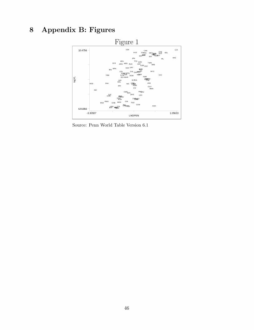
8 Appendix B: Figures

Figure 1

logY

L

LNOPEN-3.30507 1.05633

6.91856

10.4756

AGO

ARG

AUS

AUT

BDI

BEL

BEN

BFA

BGD

BLZ

BOL

BRA

BRB

BWA

CAF

CANCHE

CHL

CHN

CIV

CMR

COG

COL

COM

CPV

CRI

DNK

DOM

DZA

ECU

EGY

ESPFIN

FJI

FRA

GAB

GBR

GHA

GINGMB

GNB

GRC

GRD

GTM

GUY

HKG

HND

H TI

HUN

IDN

IND

IRL

IRN

ISLISR

ITA

JAM

JOR

JPN

KEN

KOR

LKA

LSO

LUX

MAR

MDG

MEX

MLIMOZ

MRT

MUS

MW I

MYS

NAM

NER

N GA

NIC

NLDNORNZL

PAK

PANPER

PHL

PNG

POL

PRT

PRY

ROM

RUS

RWA

SENSLE

SLV

SWE

SWZ

SYC

SYR

TCD

TGO

THA

TTO

TUNTUR

T WN

TZAUGA

URY

USA

VEN

YEM

ZAF

ZAR

Z MB

ZW E

DEU

Source: Penn World Table Version 6.1

46

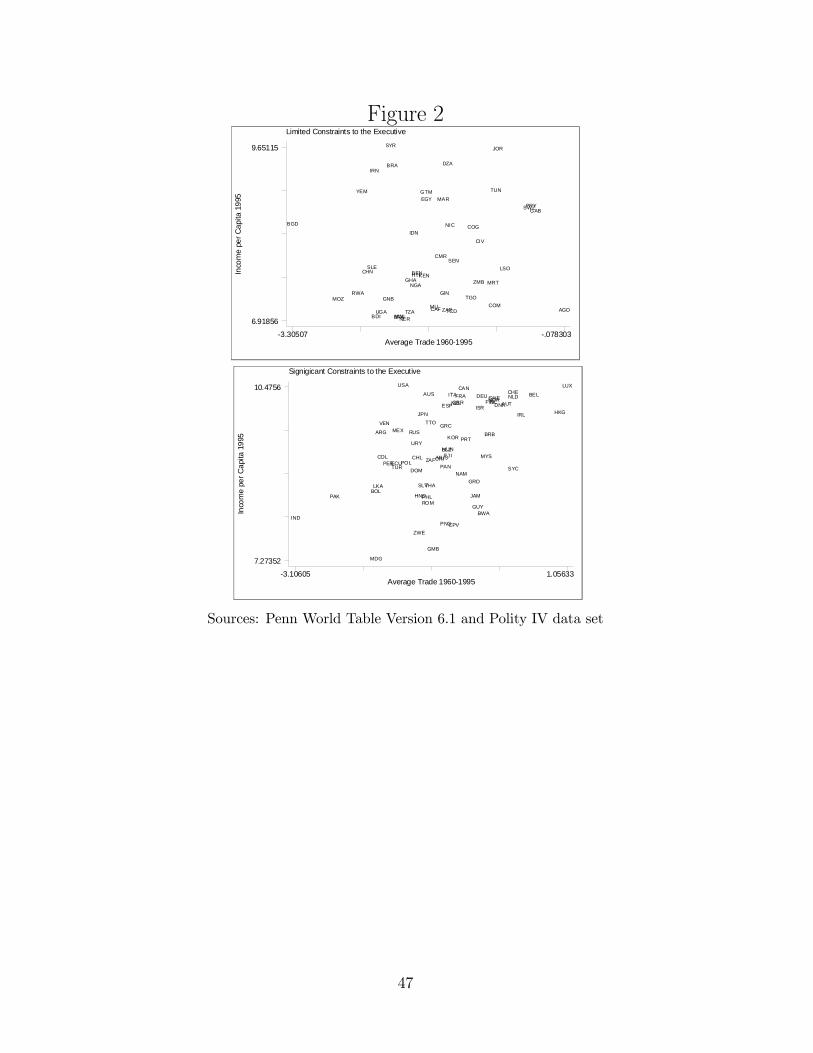
Figure 2Limited Constraints to the Executive

Inco

me

per C

apita

199

5

Average Trade 1960-1995-3.30507 -.078303

6.91856

9.65115

AGOBDI

BEN

BFA

BGD

BRA

CAF

CHN

CIV

CMR

COG

COM

DZA

EGY

GAB

GHA

GINGNB

GTM

HTI

IDN

IRN

JOR

KENLSO

MAR

MLIMOZ

MRT

MWINER

NGA

NIC

PRY

RWA

SENSLE

SWZ

SYR

TCD

TGO

TUN

TZAUGA

YEM

ZAR

ZMB

Signigicant Constraints to the Executive

Inco

me

per C

apita

199

5

Average Trade 1960-1995-3.10605 1.05633

7.27352

10.4756

ARG

AUS

AUT

BEL

BLZ

BOL

BRB

BWA

CANCHE

CHLCOL

CPV

CRI

DEU

DNK

DOMECU

ESPFIN

FJI

FRAGBR

GMB

GRC

GRD

GUY

HKG

HND

HUN

IND

IRL

ISLISR

ITA

JAM

JPN

KOR

LKA

LUX

MDG

MEX

MUS MYS

NAM

NLDNORNZL

PAK

PANPER

PHL

PNG

POL

PRT

ROM

RUS

SLV

SWE

SYC

THA

TTO

TUR

URY

USA

VEN

ZAF

ZWE

Sources: Penn World Table Version 6.1 and Polity IV data set

47