The Costs of Inefficient Robust Scheduling Practices in the U.S.

Airline Industry

Scott E. Atkinson∗ Kamalini Ramdas† Jonathan W. Williams‡

April 2013

Abstract

Airlines today use robust scheduling to plan ahead for unforeseeable disruptions. We empir-ically examine three common robust scheduling practices: flexibility to swap aircraft, flexibilityto swap gates, and scheduled downtime. To do so, we characterize efficient operating practicesin the airline industry by estimating a multiple-outcome, multiple-input production frontier.Estimates of how robust-scheduling inputs expand this frontier, and the tradeoffs faced by car-riers along this frontier, allow us to infer how carriers view the costs of robust-scheduling inputsand the value they place on various operational outcomes. These estimates provide a rationalefor the different robust scheduling practices used by carriers, point towards ways that carriersand regulators can target improvement, and demonstrate the severe consequences of even smallinefficiencies. For example, we find that on average across its network JetBlue achieves only89% of the efficient level of load factor for its observed levels of other outcomes and inputs,resulting in a 3% reduction in per-flight revenues.

Keywords: Airline Performance, Robust Scheduling, Delays, Stochastic Production Fron-tiers, Directional Distance Functions

1 Introduction

The OR literature on airline scheduling has in recent years begun to explicitly consider the impact

of disruptions on airline schedules (Rosenberger et al., 2002). Reactive disruption management

models focus on recovery from disruptions (Arguello et al., 1997), while proactive robust scheduling

approaches plan ahead for disruptions (Lan et al., 2006). Clausen et al. (2010) highlight two types

of robustness. Recovery robustness refers to the planning of schedules amenable to fast recovery

through actions such as rerouting aircraft and crews or reassigning gates, in the event of schedule

disruptions. In contrast, absorption robustness refers to the introduction of slack into airline

schedules to buffer against disruptions.

To decide on the optimal mix of robust scheduling practices, operation managers need to know

the total costs of increasing each type of robustness, which includes forgone revenues. The direct

∗Department of Economics, University of Georgia, atknsn@uga.edu.†Management Science and Operations, London Business School,kramdas@london.edu.‡Department of Economics, University of Georgia, jonwms@uga.edu.

1

costs associated with increasing robustness are known by airlines and readily observable, but the

opportunity costs of foregone revenues are far less clear (Smith and Johnson, 2006). Calculating

foregone revenues requires considering the system-wide repercussions of robust scheduling practices

on revenue derived from multiple outcomes (such as load factor, cargo, and delays), both present and

future. For example, increasing flexibility to swap aircraft and crew by having more aircraft of the

same type, e.g., Boeing 737s scheduled to depart from an airport in close proximity to one another,

can mitigate the effect of schedule disruptions. While this action incurs clearly measurable direct

costs for rerouting aircraft, the airline must also compute the opportunity cost of less-clearly-defined

foregone revenues from not deploying aircraft to depart at other times of the day or from other

airports in the airline’s network. In order to decide on the optimal level of flexibility, a manager must

weigh these costs against the future revenues generated from improved service quality (Ramdas et

al. 2013).

To infer the costs associated with robust scheduling practices, we characterize efficient operat-

ing practices in the airline industry by estimating a multiple-outcome, multiple-input production

frontier. This frontier characterizes the highest levels of good outcomes and lowest levels of bad

outcomes attainable from any given level of inputs in a specific operating environment (i.e., air-

port, time of day, and aircraft type). Estimates of the tradeoffs faced by carriers along this frontier,

combined with hand-collected data on the price of boarding gates, allow us to infer how a carrier

views the costs associated with robust-scheduling inputs and the value they place on various opera-

tional outcomes. These estimates provide a rationale for the different scheduling practices used by

carriers, and highlight ways that carriers and policy makers can target improvement. Our frontier

characterization of efficient operating practices also allows us to quantify carriers’ relative tech-

nical efficiencies, i.e., a carrier’s ability to maximize good outcomes and minimize bad outcomes

for a given level of inputs, relative to efficient practice. By doing so, we can measure the addi-

tional revenues that carriers would have realized by operating efficiently. We find that even small

inefficiencies can have severe consequences for profitability.

Our analysis builds on a growing literature in economics and operations management that has

empirically analyzed different metrics of airline performance and competition (e.g. Mazzeo 2003,

Mayer and Sinai 2003, Rupp 2009, Rupp et al. 2005, Rupp and Holmes 2006, Deshpande and

Arikan 2011, Li and Netessine 2011, Arikan et al. 2012, Cannon et al. 2012). Most of these

papers examine one performance outcome at a time, estimating the effect of different factors such

as aircraft schedules, airport concentration, network structure, or competition on the outcome in

question. Multiple performance outcomes that might impact one another are either treated as

2

separable to facilitate independent, single-equation regressions for each outcome of interest, or

as estimable using reduced-form specifications that avoid explicit joint modelling of inputs and

outcomes. Also, none of these papers consider measures of recovery robustness, the built-in ability

to swap aircraft, crew or gates when a disruption occurs.

To characterize efficient operating practices, we use a directional distance function approach

(Atkinson and Primont 2002; Atkinson and Dorfman 2005; Fare et al., 2005), which is a general-

ization of the well-established stochastic production frontier estimation method (e.g. Lieberman

and Dhawan 2005, Kumbhakar and Lovell 2000, Greene 2005). From a production theory perspec-

tive, airline service is a technology that converts inputs such as aircraft and gates into a variety of

outcomes, eventually impacting revenues and costs (Atkinson and Cornwell 1993, 1994). Since low-

cost carriers and their ”full service” (or legacy) competitors have very different operating models

or ”technologies”, point-to-point versus hub-and-spoke, we estimate an efficient operating frontier

for each carrier type.

We model three key inputs. The first, scheduled flexibility, measures an airline’s ability to swap

aircraft and crews at an airport when faced with a schedule disruption. The second, boarding gates

per scheduled departure, measures an airline’s ability to reassign gates at an airport if a schedule

disruption occurs. Finally, scheduled aircraft downtime measures the amount of planned slack in

an aircraft’s schedule. Conceptually, scheduled flexibility and gates per scheduled departure are

measures of recovery robustness, whereas scheduled downtime is a measure of absorption robustness.

To our knowledge, we are the first to empirically model airline recovery robustness, which plays an

important role in airline scheduling today.1

These inputs produce two “good” outcomes that airlines monitor closely, load factor and cargo

on passenger aircraft, and three “bad” outcomes, short, intermediate, and long flight delays. From a

theoretical perspective, considering multiple outcomes simultaneously is important if the outcomes

are non-independent. This is clearly the case for airlines. Rupp and Holmes (2006) document the

impact of load factor on delays and cancellations. Ramdas et al. (2013) report that managers at

Southwest Airlines explicitly trade off long delays for short delays.

Using our estimates of the relative returns to robust-scheduling inputs, we infer how a carrier

can trade off between inputs while keeping outcomes constant. If a carrier had sought to obtain

its observed levels of outcomes at least cost, the last dollar spent on any input must have the same

per-dollar return. Thus, with information on a single input price (gates), and estimates of the

1Rupp et al. (2005) study airlines’ recovery operations following airport closures. In contrast we examine plansput in place in advance of future disruptions.

3

tradeoffs amongst inputs, we can infer how a carrier must have viewed the prices of other inputs,

which are not directly observable.

We estimate the median cost of increasing flexibility to swap aircraft by one unit, i.e., of in-

creasing by one the number of flights of a particular aircraft type departing at a particular time of

day, to be five times greater for legacy carriers than for low-cost carriers, $961 versus $172. Our

conversations with airline operations managers suggest that low cost carriers use homogenous fleets

and concentrated operations on high-density routes to lower the cost of flexibility. In contrast, the

constraints that legacy carriers face in facilitating passenger connections in their networks raise

the cost of flexibility. We also find that the median per-minute cost of scheduled downtime for

low-cost carriers is more than twice that for legacy carriers, $17 versus $8, which rationalizes the

much tighter aircraft schedules used by low-cost carriers. The networks for legacy or hub-and-spoke

carriers are more highly connected than those for low-cost or point-to-point carriers. This higher

level of connectivity implies that legacy carriers forgo less revenue when downtime is increased,

since it facilitates additional passenger connections. The very different estimates of the costs of

robust-scheduling inputs for low cost and legacy carriers are consistent with their observed schedul-

ing practices, suggesting that carriers appear to choose the least cost set of inputs to produce their

observed outcomes. To our knowledge, no prior research empirically estimates the costs of recovery

robustness in the airline industry.

Our estimates of the costs of robust-scheduling inputs highlight ways that carriers can target

improvement. If a carrier’s true input costs differ from our estimates, it can reallocate inputs to

become more profitable by choosing a different mix of inputs (i.e., achieve allocative efficiency).2

For example, consider JetBlue’s operations at Boston Logan. If JetBlue’s true per-minute cost of

downtime was 5% higher than its behavior suggests (e.g., JetBlue overvalues facilitating connections

at Logan), then JetBlue should have been using significantly less downtime while increasing its use

of other less expensive inputs. One option would be to use gates more intensively. JetBlue could

increase the number of flights by 5% with no adverse consequences for good outcomes (i.e load

factor and cargo) or bad outcomes (i.e., delays). JetBlue operated 1760 flights from Boston Logan

in December 2009 and its average per-flight revenues were $64, 544.73,3 implying $5, 679, 936.24 in

forgone revenue in that month alone. This highlights the importance of accurately estimating the

costs of robust-scheduling inputs.

We are also able to identify the tradeoffs between any two outcomes for efficient low-cost and

2Olivares et al. (2008) perform a similar calculation for hospitals seeking to efficiently schedule hospital operatingrooms.

3Source: JetBlue’s 2009 annual report.

4

legacy carriers. For example, we can estimate the decrease in load factor required to improve

on-time performance by a given amount, keeping inputs and other outcomes constant. Since the

cost associated with enplaning one more passenger is relatively easily quantified - by fare paid -

we can infer the value that a carrier places on marginal improvements in on-time performance.

We estimate that JetBlue forgoes 0.57 additional passengers at an average fare of $130.41 for a

marginal improvement of 1% in on-time performance. This corresponds to $74.33 per flight, or

0.48% of revenues on an average flight.4 Therefore if an airline’s true cost to improve on-time

performance is lower than our estimate, it may be able to increase profits by repositioning itself to

offer better on-time performance.

Our characterization of the efficient frontier can also guide airline policy, which must balance

the benefits to passengers of fewer delays against the costs to carriers of limiting the severity and

frequency of delays. Recent work in economics, Snider and Williams (2013), suggests that current

federal policy which limits airports’ ability to raise capital to expand airport facilities both limits

competition and worsens the frequency and length of delays. Our estimates give policy makers

insight into the costs that carriers would incur if forced amend scheduling practices to reduce

delays. These can then be weighed against the costs of alternative ways to reduce delays, such

as building additional airport facilities to alleviate congestion (Daniel 1995). Currently, as part of

the FAA Modernization and Reform Act of 2012 (Section 406(b)), the DOT is conducting such a

review of “carrier flight delays, cancellations, and associated causes...”. This includes assessing “air

carriers’ scheduling practices”, “capacity benchmarks at the Nation’s busiest airports”, and give

“recommendations for programs that could be implemented to address the impact of flight delays

on air travelers”.

Finally, our structural estimates of the production frontier for each carrier type enable us to

provide measures of technical efficiency, i.e., to quantify carriers’ ability to maximize good outcomes

and minimize bad outcomes for a given level of inputs. While Southwest is often touted for its

efficient operations, i.e., the ”Southwest effect”, our results reveal that once we control for input

choices and environmental factors, any presumed superiority is largely explained away. When other

carriers employ similar levels of inputs and operate in the same environments, they often perform

at least as well as Southwest. In fact, among low-cost carriers, we find that AirTran performs better

than Southwest for each measure of delays, demonstrating the importance of accounting for the

operating environment when evaluating carriers’ operations.

4Shumsky (1993) demonstrates the responsiveness of carriers to the On-Time Disclosure rule, which is consistentwith our finding that carriers place significant value on improving delays.

5

The lost revenues from utilizing inputs inefficiently are substantial. For example, we estimate

that on average across its network JetBlue achieved only 89% of the efficient level of load factor,

given its observed levels of other outcomes and inputs. This implies that JetBlue’s inefficiencies cost

up to $1926.80 dollars on an average flight, corresponding to 3% of per-flight revenues. Given the

low marginal costs associated with transporting additional passengers on a flight, this corresponds

to a significant loss in profitability.

The rest of this paper is organized as follows. Section 2 describes our data. The details of the

structural directional distance econometric model are discussed in Section 3. Section 4 presents our

results, and Section 5 concludes.

2 Data

We use three data sources from the Bureau of Transportation Statistics (BTS): the on-time per-

formance database, the B43 form on aircraft inventories, and the T100 segment database. Other

data we use in our analysis includes information on airlines’ lease payments to airports from FAA

Form 127, and a survey on carrier-specific access to airport facilities conducted jointly with North

America’s largest airport trade organization, the ACI-NA (see Williams 2012). We discuss how

each source of data is used below.

2.1 On-Time Performance Data

The BTS on-time performance database allows us to compare carriers’ operational performance

in the same environment (i.e., airport, day of week, and departure time block) while operating

similar equipment (i.e., aircraft type) at each point in time (i.e., year and month). Let i = 1, ...., I

represent a particular environment, i.e., a unique combination of airport (e.g., Atlanta Hartsfield

or ATL), day of week (e.g., Monday), and scheduled departure time block (e.g., 10am-2pm EST),

j = 1, ..., J a carrier (e.g., Delta), k = 1, ...,K an aircraft type (e.g., Boeing 737), and t = 1, ..., T a

year and month (e.g., January 2009). Our unit of analysis is the 4-tuple (i, j, k, t). We group flights

into 4 different departure time blocks; midnight-10am (morning), 10am-2pm (midday), 2pm-6pm

(afternoon), and 6pm-midnight (evening). For aircraft types, we proxy using an aircraft’s crew-

rating.5 To focus on only domestic service, we eliminate from our sample all aircraft that appear

to be involved in international service.6 Using this data, we calculate three different bad outcomes,

5In all but a few cases, a crew-rating corresponds to a single aircraft type, so we use the two terms interchangeably.6To do this, we first merge, by tail number, the BTS on-time performance database with aircraft information in

the BTS B43 form. We then remove aircraft equipped for international travel, i.e., flying over large water bodies.Next, we remove aircraft that appear to have flown an international segment, identified via gaps in the aircraft’s

6

which are quantiles of the departure delays distribution for each 4-tuple, (i, j, k, t):

P(> 15)ijkt is the proportion of flights flown in environment i by carrier j using equipment k in

time period t that departed 15 or more minutes late. P(> 60)ijkt and P(> 180)ijkt are similarly

defined. The variable P(> 15)ijkt is identical to the DOT’s prominently reported measure of

on-time performance, while the other two measures above capture the shape of the tail of the

delays distribution.7

We use the detail of the on-time performance database to track each aircraft’s routing, which

we use to calculate two input variables:

Downtimeijkt is the average number of minutes between an aircraft’s scheduled arrival and its

next scheduled departure, or average scheduled downtime, taken over all departures in 4-tuple,

(i, j, k, t). We use scheduled downtime as a measure of absorption robustness. In keeping with the

ex ante planning inherent in robust scheduling, scheduled downtime is by definition determined

at the schedule planning stage, and is therefore a good measure of absorption robustness.

Flexijkt is the total number of aircraft of type k belonging to carrier j that are scheduled to

depart from environment i in time period t. An increased number of aircraft of the same aircraft

type give a carrier additional flexibility to substitute aircraft and crews when needed. Scheduled

flexibility is our first measure of recovery robustness. It is conceptually similar to the “station

purity” measure of Smith and Johnson (2006).8

In estimating a production frontier, one must carefully control for both the operating environ-

ment and the operating model or ”technology” of the firms in question. In the airline industry,

the operating environment varies widely even within an airport. We difference out time-invariant

factors unique to each operating environment i, characterized by time of day and day of week at

a particular airport. To capture differences across carriers, j, we include carrier dummies. We

also control for aircraft type, k, using aircraft-type dummies, since different aircraft types may

be affected differently by the same airport conditions (e.g. larger aircraft may get preference in

a departure queue). We include region-month dummies to control for seasonal weather patterns

for each of 5 regions: Midwest, Northeast, Northwest, Southeast, and Southwest. We also include

year-month dummies, t, to control for common trends over time across all carriers. In Section 3.2,

routing. Finally, we remove obvious reporting errors such as aircraft that report an infeasible flight sequence.7Cancellations are treated as delays of longer than 180 minutes and included in each of the measures above.8Flights scheduled to depart at a similar time and using the same aircraft type may not always be able to swap

aircraft or crew. Scheduled maintenence and limitations on crew hours make our measure an upper bound onflexibility. Our empirical approach, which exploits variation within an environment (i) to identify model parameters,removes the average effect of any systematic upward bias in flexibility within an environment.

7

we discuss how we account for the different tradeoffs encountered by ”full service” legacy carriers

and more focused low-cost carriers.

We control for variation in market concentration and congestion over time within each environ-

ment i with these variables:

HHIit is the Herfindahl-Hirschman index for scheduled departures in the departure time-block,

day-of-week, and airport that characterize environment i in time period t. Carriers have a

greater incentive to reduce delays when airport concentration, HHIit, increases because more

of the costs of delays are realized by the carrier itself (Mayer and Sinai 2003; Brueckner 2002,

2005). Therefore we expect the frontier to be characterized by a lower level of delays in more

concentrated environments.

Congestionit is the total number of flights scheduled to depart in the time-block, day-of-week,

and airport that characterize environment i in time period t.

After constructing these variables, we limit our sample to 4-tuples (i, j, k, t) for which at least ten

flights were used to construct each of the variables described above. Essentially, we consider a

carrier j to serve a particular environment i - characterized by a specific airport, departure time

block and day of week - with aircraft type k in year-month t, if there were at least ten departures

in (i, j, k, t).9

2.2 T100 Data

The BTS T100 domestic-segment database contains detailed information on passenger volumes,

cargo, and available seats by airport of origin, carrier, aircraft type, month, and year. For each

4-tuple, (i, j, k, t), we use these data to calculate two good outcomes:

LoadFactorijkt is the proportion of available seats filled by revenue-generating passengers,

averaged over all departures in (i, j, k, t).

Cargoijkt is the average cargo, i.e., sum of weights of freight and mail transported, in tens of

thousands of pounds per scheduled departure, averaged over all departures in (i, j, k, t).

By including cargo as an outcome we can explicitly credit carriers that increase cargo conditional

on inputs and other outcomes. Note that LoadFactor and Cargo are obtained from the T100

dataset which is not specific as to the day of week or departure time block in which each aircraft

departs.

9Our results are insensitive to varying this cutoff in either direction.

8

2.3 FAA Form 127 and ACI-NA Airport Survey

Our data on boarding gates come from a recent survey on access to airport facilities conducted

jointly with the ACI-NA (Ciliberto and Williams 2010, Williams 2012, Snider and Williams 2012),

which reports information on carriers’ access to boarding gates during 1997, 2001, 2007, 2008 and

2009. Gate leases are of two types. An exclusive lease gives a carrier the right to use a gate and to

deny its use to other carriers. A preferential lease gives a carrier first right to a gate, and no right

to deny others its use when lying unused. From these data, for each 3-tuple, (i, j, t) we construct

a third input variable:

GatesSchedDepijt is the total number of gates leased to carrier j on either an exclusive or

preferential basis at the airport pertaining to environment i in time period t, divided by the

number of scheduled departures pertaining to (i, j, t). Since we do not know the operational

limitations of the gates leased to each carrier, such as ability to handle particular aircraft,

GatesSchedDepijt does not vary with k.

We also collect unique detailed data on costs associated with leasing airport facilities from the

FAA’s Form 127 for 2009.10 For each airport, we use this data to construct one additional variable:

GatePriceijt is the total monthly fees paid by carrier j to airport i for terminal leases and

apron fees divided by the number of gates leased by the carrier at the airport.11

2.4 Final Sample and Descriptive Statistics

After merging the datasets described above by unique 4-tuples (i, j, k, t), we have 172,380 observa-

tions, drawn from 81 airports, all of which are in the top 100 airports by passenger enplanements

in the years in which we have survey data on boarding gates: 1997, 2001, 2007, 2008, and 2009.

The carriers in our final sample are American (AA), JetBlue (B6), Continental (CO), Delta (DL),

Frontier (F9), Airtran (FL), Northwest (NW), United (UA), US Air (US), and Southwest (WN).12

Table 1 contains summary statistics, by carrier and year.

We find starker differences among the carriers in the levels of inputs, than in outcomes. On

average, low-cost carriers schedule half the downtime of their legacy competitors, with Southwest

responsible for the majority of this difference. Other low-cost carriers, which have more network

overlap with their legacy competitors and operate in the same large hubs, (e.g., AirTran in Atlanta

10http://cats.airports.faa.gov/Reports/reports.cfm11The apron is the area of an airport where aircraft are parked, unloaded or loaded, refueled, and boarded.12We drop Alaska (AS) because its regional nature and limited range of service match up poorly with the responses

to the gates survey data, and America West (HP) because its merger with USAir limits its data to the first twosample years, and it dramatically reduced its destinations served following a bankruptcy in the mid-1990s.

9

Off Peak Peak Off Peak Peak0

0.05

0.1

0.15

0.2

0.25

0.3

0.35

0.4

0.45

0.5

GatesPer

ScheduledDeparture

Legacy

Low-Cost

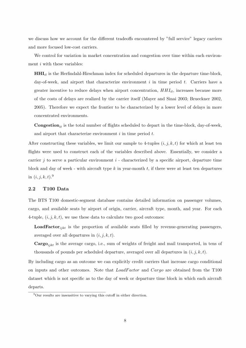
Figure 1: Gate Utilization by Carrier Type and Time of Day

Hartsfield) tend to schedule downtimes more similar to those of legacy carriers. Regarding flexibility,

low-cost carriers tend to schedule more aircraft of the same type to depart an airport in the same

time block and day of week, despite operating at airports that are substantially smaller on average.

We find that low-cost carriers tend to use gates much more intensively, i.e., with a lower ratio

of gates to scheduled departures. Figure 1 gives the mean of GatesSchedDepijt by carrier type

and time of day. Peak is defined as the middle two 4-hour time blocks, while off peak includes

the first and last time block. Legacy carriers use gates less intensively at all times, but experience

a much greater change in gate utilization during peak hours. Table 1 also shows that low-cost

carriers, particularly JetBlue and Southwest, tend to concentrate their operations in less congested

yet more concentrated airports, which gives them tremendous flexibility to shuffle departures across

gates to minimize delays(see Mayer and Sinai 2003).

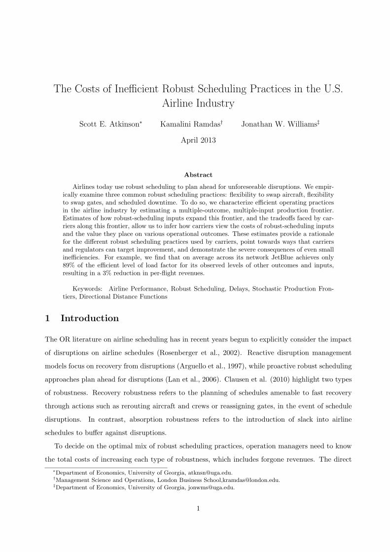
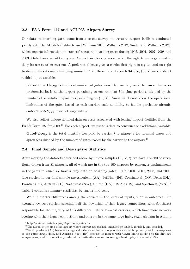
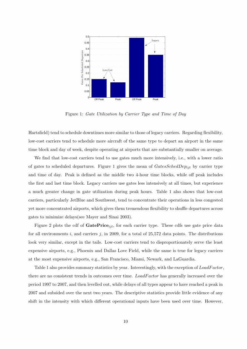
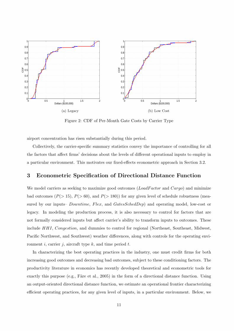
Figure 2 plots the cdf of GatePriceijt, for each carrier type. These cdfs use gate price data

for all environments i, and carriers j, in 2009, for a total of 25,572 data points. The distributions

look very similar, except in the tails. Low-cost carriers tend to disproportionately serve the least

expensive airports, e.g., Phoenix and Dallas Love Field, while the same is true for legacy carriers

at the most expensive airports, e.g., San Francisco, Miami, Newark, and LaGuardia.

Table 1 also provides summary statistics by year. Interestingly, with the exception of LoadFactor,

there are no consistent trends in outcomes over time. LoadFactor has generally increased over the

period 1997 to 2007, and then levelled out, while delays of all types appear to have reached a peak in

2007 and subsided over the next two years. The descriptive statistics provide little evidence of any

shift in the intensity with which different operational inputs have been used over time. However,

10

0 0.5 1 1.5 20

0.1

0.2

0.3

0.4

0.5

0.6

0.7

0.8

0.9

1

Dollars ($100,000)

CD

F

(a) Legacy

0 0.5 1 1.5 20

0.1

0.2

0.3

0.4

0.5

0.6

0.7

0.8

0.9

1

Dollars ($100,000)

CD

F

(b) Low Cost

Figure 2: CDF of Per-Month Gate Costs by Carrier Type

airport concentration has risen substantially during this period.

Collectively, the carrier-specific summary statistics convey the importance of controlling for all

the factors that affect firms’ decisions about the levels of different operational inputs to employ in

a particular environment. This motivates our fixed-effects econometric approach in Section 3.2.

3 Econometric Specification of Directional Distance Function

We model carriers as seeking to maximize good outcomes (LoadFactor and Cargo) and minimize

bad outcomes (P (> 15), P (> 60), and P (> 180)) for any given level of schedule robustness (mea-

sured by our inputs– Downtime, Flex, and GatesSchedDep) and operating model, low-cost or

legacy. In modeling the production process, it is also necessary to control for factors that are

not formally considered inputs but affect carrier’s ability to transform inputs to outcomes. These

include HHI, Congestion, and dummies to control for regional (Northeast, Southeast, Midwest,

Pacific Northwest, and Southwest) weather differences, along with controls for the operating envi-

ronment i, carrier j, aircraft type k, and time period t.

In characterizing the best operating practices in the industry, one must credit firms for both

increasing good outcomes and decreasing bad outcomes, subject to these conditioning factors. The

productivity literature in economics has recently developed theoretical and econometric tools for

exactly this purpose (e.g., Fare et al., 2005) in the form of a directional distance function. Using

an output-oriented directional distance function, we estimate an operational frontier characterizing

efficient operating practices, for any given level of inputs, in a particular environment. Below, we

11

describe the theoretical properties that we will impose on this function during estimation, in order

to ensure a well-defined production technology.

3.1 Theoretical Properties

Consider an airline production technology by which firms combine multiple operational inputs,

x = (x1, . . . , xN ) ∈ RN+ , to produce multiple good outcomes, y = (y1, . . . , yM ) ∈ RM

+ , and bad

outcomes, y = (y1, . . . , yL) ∈ RL+. The firm’s production technology, P (x,y,y), can be written as

P (x,y,y) = {(x, y, y) : x can produce y and y}, (1)

where P (x,y,y) consists of all feasible input and outcome vectors.

Following Chambers et al., (1998) and Fare et al., (2005), we define the output-oriented direc-

tional distance function as

−→Do(x,y, y,gy,−gy) = β∗ = sup

β{β : (y + βgy, y − βgy) ∈ P (x,y,y)}. (2)

This function,−→Do(x,y, y,gy,−gy), provides a measure of the increase in good outcomes and de-

crease in bad outcomes needed to move a carrier to the frontier of the production set, P (x,y,y), for

a given level of inputs. Thus, a carrier’s distance from the frontier is the addition to good outcomes

and the reduction of bad outcomes required to reach the frontier in a direction given by the vector,

(gy = 1,−gy = 1).

As discussed in Chambers et al., (1998), the output-oriented directional distance function,−→Do(x,y, y,gy,−gy), defined in Equation 2 must satisfy the following properties:

Non-Negativity:

−→Do(x,y, y,gy,−gy) ≥ 0 ⇐⇒ (y, y) ∈ P (x,y,y). (P1)

Property P1 requires that the output-oriented directional distance function be non-negative,

with the most efficient firm having−→Do(x,y, y,gy,−gy) = 0. We ensure this property is satisfied

via a normalization of the fitted function.

Translation Property:

−→Do(x,y + αgy, y − αgy,gy,−gy) =

−→Do(x,y, y,gy,−gy)− α. (P2)

Property P2 is true by definition of the output-oriented directional distance function, Equation

(2). This property implies that increasing y and decreasing y by α, multiplied by their respective

12

directions, holding inputs constant, will result in a decrease in the output directional distance by

α, and therefore an increase in efficiency equal to α. We ensure that Property (P2) is satisfied

via the parametric restrictions that are imposed during estimation and described in Section

3.2.13

g-Homogeneity of Degree Minus One:

−→Do(x,y, y, λgy,−λgy) = λ−1−→Do(x,y, y,gy,−gy), λ > 0. (P3)

Property P3 also follows directly from Equation (2), since scaling each element of the direction

vector, (gy = 1,−gy = 1), by λ will scale the output directional distance by λ−1. Multiplying

gy and gy by λ divides β∗ by λ. Property P3 is satisfied once P2 is imposed (via parametric

restrictions) and the model is estimated as described in Section 3.2.

Good Outcome Monotonicity:

y′ ≥ y → −→Do(x,y

′, y,gy,−gy) ≤−→Do(x,y, y,gy,−gy). (P4a)

and

Bad Outcome Monotonicity

y′ ≥ y →−→Do(x,y, y

′,gy,−gy) ≥−→Do(x,y, y,gy,−gy). (P4b)

Properties P4a and P4b state that the output-oriented directional distance function is monoton-

ically decreasing in good outcomes, while it is monotonically increasing in bad outcomes. That

is, holding all else constant, increasing a good outcome (or decreasing a bad outcome) moves

the directional distance function closer to zero, i.e., the carrier becomes more efficient. We test

for Properties P4a and P4b in Section 4 and find that they are satisfied, so that we do not need

to impose them during estimation.

3.2 Econometric Methodology

We estimate a directional distance function using a variant of fixed-effects estimation in which the

coefficients estimated are subject to a set of parametric restrictions that satisfy Properties P1-P4b.

A major benefit of this approach, as discussed below, is that we can remove time-invariant sources

of endogeneity from our model specification.

13These parametric restrictions are analogous to imposing linear homogeneity when estimating a cost function (e.g.,Equation (2) in Berndt and Wood, 1975).

13

We model three bad outcomes, yijkt, which are quantiles of the departure delays distribution

(P (> 15)ijkt, P (> 60)ijkt, and P (> 180)ijkt), and two good outcomes, yijt, LoadFactorijt and

Cargoijt. The operational inputs are Flexijkt, Downtimeijkt, and GatesSchedDepijt. We also

include other factors alluded to above and discussed below that can affect the production relation-

ship. To capture the differences in the operating models of low-cost and legacy carriers, we specify

a flexible piece-wise linear functional form for the output-oriented directional distance function

(dropping the o subscript) that allows for different coefficients for each carrier type:

0 =−→D t(xijkt,yijkt, yijkt,wit,dijkt;gy,−gy, γ, ϕ, η, λ) + εijkt, (3)

where

−→D t(xijkt,yijkt, yijkt,wit,dijkt;gy,−gy, γ, ϕ, η, λ)

=M∑

m=1

(γmy + ϕm

y dLeg)ymijkt +

L∑l=1

(γly + ϕl

ydLeg

)ylijkt (4)

+

N∑n=1

(γnx + ϕnxdLeg)x

nijkt + (γw+ϕwdLeg)wit

+ηaircraftk daircraftk + ηyr−mont dyr−mon

t + ηreg−monr dreg−mon

r

+ηcarrierj dcarrierj + λLcci + λLeg

i

and

εijkt = υijkt − uijkt.

As is customary in directional distance function estimation (Fare et al., 2005), the left-hand side

of Equation 4 is set equal to zero, representing frontier production. Thus, a carrier on the frontier

will have a fitted distance of zero.

Following Kumbhakar and Lovell (2000) and Fare et al., (2005), we decompose the error term,

εijkt, into a one-sided component, uijkt > 0, that captures unmeasured time-varying differences in

carriers’ managerial ability or operational difficulties unique to specific carriers,14 and a two-sided

mean-zero idiosyncratic component, υijkt, that allows for random and transitory shocks impacting

carriers’ ability to transform inputs to outcomes, such as poor weather. We make no parametric

distributional assumptions for either error.

14Note that we have removed time-invariant firm-specific unobserved heterogeneity from uijkt by including carrierdummies dcarrierj in the regression model.

14

The flexibility in the functional form and inclusion of the dummy variables dijkt (daicraftk ,

dyr−mont , dreg−mon

r , and dcarrierj ), wit (Congestionit and HHIit), and fixed effects for each envi-

ronment and carrier type (λLcci and λLeg

i ) eliminates sources of endogeneity, i.e., unobserved de-

terminants of carriers’ input choices and outcomes. Since our three robust-scheduling inputs are

scheduled well in advance, fixed effects are an appropriate way to remove potential endogeneity.

Our functional form allows for the return to inputs, tradeoff between outcomes, and impact of

environmental factors to vary with the operating model (low-cost or legacy) of each carrier j via

the interactions with the legacy carrier-type dummy, dLeg, which takes on a value of one for legacy

carriers and zero otherwise. The dummy variables, daicraftk , dyr−mont , dreg−mon

r , and dcarrierj , re-

move time-invariant unobservables for each aircraft-type, year-month, region-month, and carrier,

respectively.15 The region-month dummies, which control for differential weather patterns across

regions, Congestionit, and HHIit allow for the frontier to be characterized by lower levels of good

outcomes and higher levels of bad outcomes from the same level of inputs in more difficult envi-

ronments. The fixed effects, λLcci and λLeg

i , control for time-invariant unobservables specific to

environment i for low-cost and legacy carriers, respectively.

For each carrier type, we remove time-invariant unobservables specific to environment i, λLcci and

λLegi , by subtracting from each variable in Equation 4 its mean value for environment i to obtain

a transformed distance function,−→D−

t (xijkt,yijkt, yijkt,wit,dijkt;gy,−gy, γ, ϕ, η). We employ this

procedure rather than the equivalent method of estimating over 4000 unique coefficients, one for

each environment and carrier type.

Since Equation (4) characterizes a directional distance function that measures a carrier’s distance

from a production frontier, we expect a positive sign for each of the inputs. For example, an increase

in Gates, holding all outcomes and other inputs constant, should increase a carrier’s distance

from the production frontier, as it entails using more inputs to achieve a given level of outcomes.

Similarly, we expect a negative (positive) sign for the coefficient on each good (bad) outcome. A

carrier that increases a good (bad) outcome, holding all other outcomes and inputs constant, has

reduced (increased) its distance from the frontier, consistent with Property P4a (P4b).

Similar to Atkinson and Primont (2002) and Fare et al. (2005), our parameter estimates satisfy

{γ,ϕ, η} =argmin{γ,ϕ,η}

∑i,j,k,t

(0−

−→D−

t (xijkt,yijkt, yijkt,wit,dijkt;gy,−gy, γ, ϕ, η))2

, (5)

subject to

15A subset of the dummy variables must be dropped due to linear dependence (e.g., a low-cost carrier operatingone type of aircraft in a region in a particular month).

15

i)−→D−

t (xijkt,yijkt, yijkt,wit,dijkt;gy,−gy, γ, ϕ, η) ≥ 0, for all (i,j,k,t)

ii)∂−→D−

t (xijkt,yijkt,yijkt,wit,dijkt;gy,−gy ,γ,ϕ,η)∂ym

≥ 0

iii)∂−→D−

t (xijkt,yijkt,yijkt,wit,dijkt;gy ,−gy,γ,ϕ,η)∂xm

≥ 0

iv)∂−→D−

t (xijkt,yijkt,yijkt,wit,dijkt;gy ,−gy ,γ,ϕ,η)∂ym

≤ 0

v)M∑

m=1γmy gy −

L∑l=1

γlygy = 0

vi)M∑

m=1

(γmy + ϕm

y

)gy −

L∑l=1

(γly + ϕl

y

)gy = 0.

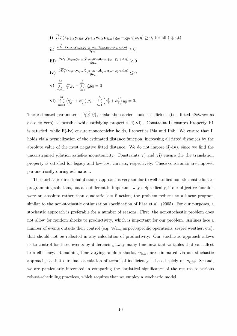
The estimated parameters, {γ,ϕ, η}, make the carriers look as efficient (i.e., fitted distance as

close to zero) as possible while satisfying properties i)-vi). Constraint i) ensures Property P1

is satisfied, while ii)-iv) ensure monotonicity holds, Properties P4a and P4b. We ensure that i)

holds via a normalization of the estimated distance function, increasing all fitted distances by the

absolute value of the most negative fitted distance. We do not impose ii)-iv), since we find the

unconstrained solution satisfies monotonicity. Constraints v) and vi) ensure the the translation

property is satisfied for legacy and low-cost carriers, respectively. These constraints are imposed

parametrically during estimation.

The stochastic directional-distance approach is very similar to well-studied non-stochastic linear-

programming solutions, but also different in important ways. Specifically, if our objective function

were an absolute rather than quadratic loss function, the problem reduces to a linear program

similar to the non-stochastic optimization specification of Fare et al. (2005). For our purposes, a

stochastic approach is preferable for a number of reasons. First, the non-stochastic problem does

not allow for random shocks to productivity, which is important for our problem. Airlines face a

number of events outside their control (e.g. 9/11, airport-specific operations, severe weather, etc),

that should not be reflected in any calculation of productivity. Our stochastic approach allows

us to control for these events by differencing away many time-invariant variables that can affect

firm efficiency. Remaining time-varying random shocks, υijkt, are eliminated via our stochastic

approach, so that our final calculation of technical inefficiency is based solely on uijkt. Second,

we are particularly interested in comparing the statistical significance of the returns to various

robust-scheduling practices, which requires that we employ a stochastic model.

16

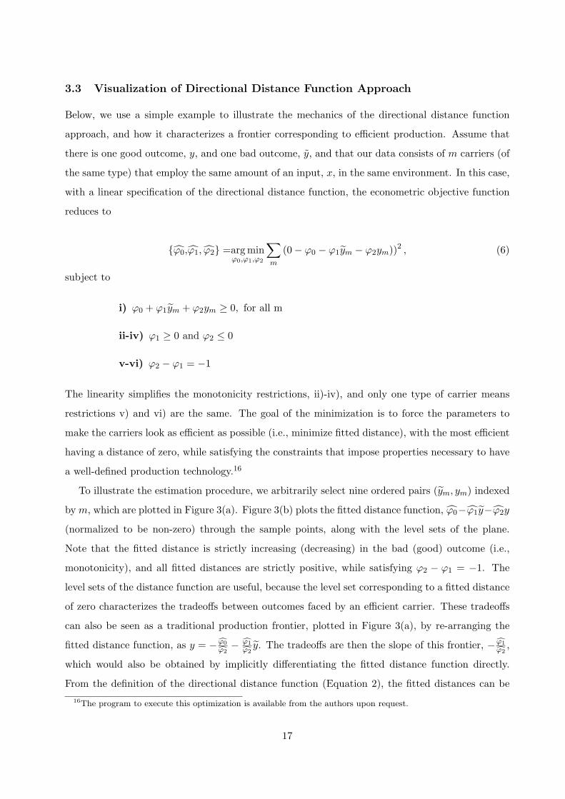
3.3 Visualization of Directional Distance Function Approach

Below, we use a simple example to illustrate the mechanics of the directional distance function

approach, and how it characterizes a frontier corresponding to efficient production. Assume that

there is one good outcome, y, and one bad outcome, y, and that our data consists of m carriers (of

the same type) that employ the same amount of an input, x, in the same environment. In this case,

with a linear specification of the directional distance function, the econometric objective function

reduces to

{φ0,φ1, φ2} =argminφ0,φ1,φ2

∑m

(0− φ0 − φ1ym − φ2ym))2 , (6)

subject to

i) φ0 + φ1ym + φ2ym ≥ 0, for all m

ii-iv) φ1 ≥ 0 and φ2 ≤ 0

v-vi) φ2 − φ1 = −1

The linearity simplifies the monotonicity restrictions, ii)-iv), and only one type of carrier means

restrictions v) and vi) are the same. The goal of the minimization is to force the parameters to

make the carriers look as efficient as possible (i.e., minimize fitted distance), with the most efficient

having a distance of zero, while satisfying the constraints that impose properties necessary to have

a well-defined production technology.16

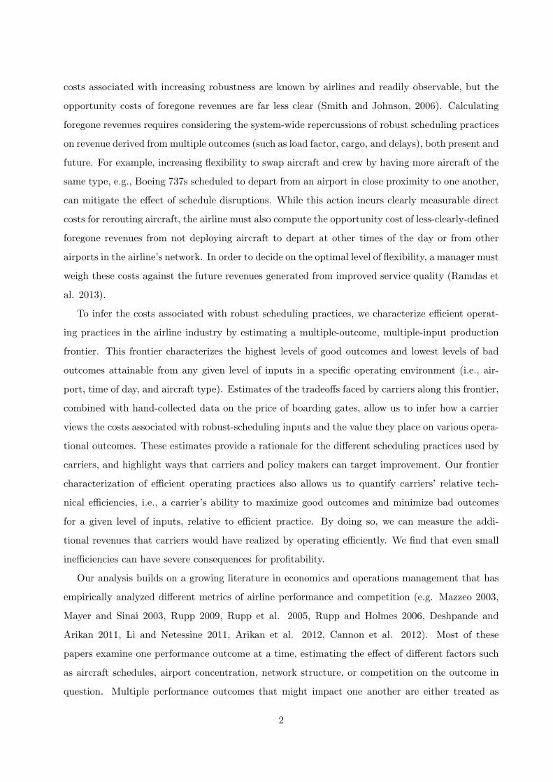
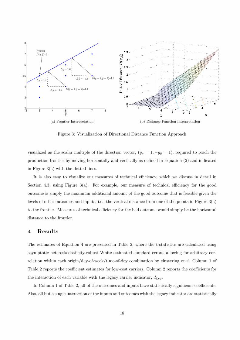
To illustrate the estimation procedure, we arbitrarily select nine ordered pairs (ym, ym) indexed

by m, which are plotted in Figure 3(a). Figure 3(b) plots the fitted distance function, φ0−φ1y−φ2y

(normalized to be non-zero) through the sample points, along with the level sets of the plane.

Note that the fitted distance is strictly increasing (decreasing) in the bad (good) outcome (i.e.,

monotonicity), and all fitted distances are strictly positive, while satisfying φ2 − φ1 = −1. The

level sets of the distance function are useful, because the level set corresponding to a fitted distance

of zero characterizes the tradeoffs between outcomes faced by an efficient carrier. These tradeoffs

can also be seen as a traditional production frontier, plotted in Figure 3(a), by re-arranging the

fitted distance function, as y = − φ0

φ2− φ1

φ2y. The tradeoffs are then the slope of this frontier, − φ1

φ2,

which would also be obtained by implicitly differentiating the fitted distance function directly.

From the definition of the directional distance function (Equation 2), the fitted distances can be

16The program to execute this optimization is available from the authors upon request.

17

2 3 4 5 6 7 82

3

4

5

6

7

8

y

y

D(y = 5, y = 7)=1.6

∆y = 1.6

D(y = 4, y = 5)=1.4

∆y = 1.4

∆y = −1.4

∆y = −1.6

FrontierD(y, y)=0

(a) Frontier Interpretation (b) Distance Function Interpretation

Figure 3: Visualization of Directional Distance Function Approach

visualized as the scalar multiple of the direction vector, (gy = 1,−gy = 1), required to reach the

production frontier by moving horizontally and vertically as defined in Equation (2) and indicated

in Figure 3(a) with the dotted lines.

It is also easy to visualize our measures of technical efficiency, which we discuss in detail in

Section 4.3, using Figure 3(a). For example, our measure of technical efficiency for the good

outcome is simply the maximum additional amount of the good outcome that is feasible given the

levels of other outcomes and inputs, i.e., the vertical distance from one of the points in Figure 3(a)

to the frontier. Measures of technical efficiency for the bad outcome would simply be the horizontal

distance to the frontier.

4 Results

The estimates of Equation 4 are presented in Table 2, where the t-statistics are calculated using

asymptotic heteroskedasticity-robust White estimated standard errors, allowing for arbitrary cor-

relation within each origin/day-of-week/time-of-day combination by clustering on i. Column 1 of

Table 2 reports the coefficient estimates for low-cost carriers. Column 2 reports the coefficients for

the interaction of each variable with the legacy carrier indicator, dLeg.

In Column 1 of Table 2, all of the outcomes and inputs have statistically significant coefficients.

Also, all but a single interaction of the inputs and outcomes with the legacy indicator are statistically

18

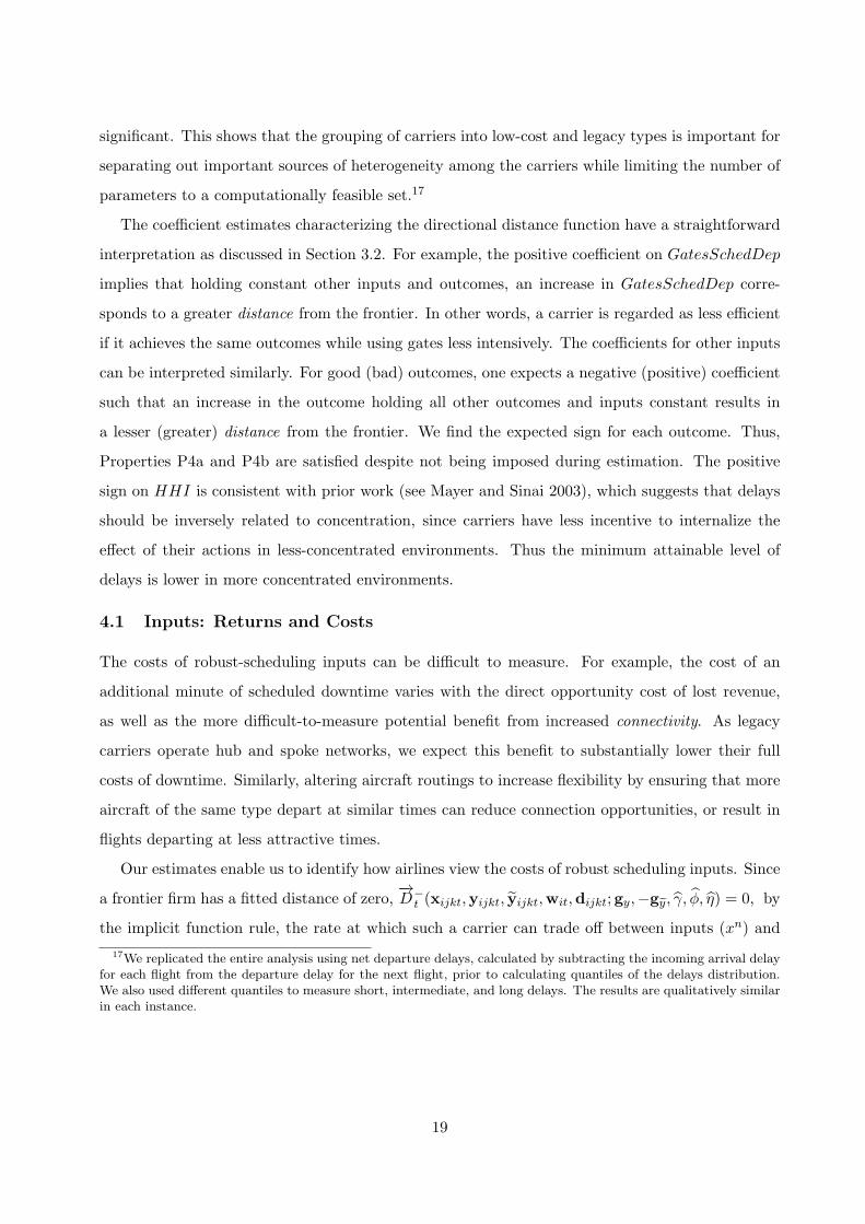
significant. This shows that the grouping of carriers into low-cost and legacy types is important for

separating out important sources of heterogeneity among the carriers while limiting the number of

parameters to a computationally feasible set.17

The coefficient estimates characterizing the directional distance function have a straightforward

interpretation as discussed in Section 3.2. For example, the positive coefficient on GatesSchedDep

implies that holding constant other inputs and outcomes, an increase in GatesSchedDep corre-

sponds to a greater distance from the frontier. In other words, a carrier is regarded as less efficient

if it achieves the same outcomes while using gates less intensively. The coefficients for other inputs

can be interpreted similarly. For good (bad) outcomes, one expects a negative (positive) coefficient

such that an increase in the outcome holding all other outcomes and inputs constant results in

a lesser (greater) distance from the frontier. We find the expected sign for each outcome. Thus,

Properties P4a and P4b are satisfied despite not being imposed during estimation. The positive

sign on HHI is consistent with prior work (see Mayer and Sinai 2003), which suggests that delays

should be inversely related to concentration, since carriers have less incentive to internalize the

effect of their actions in less-concentrated environments. Thus the minimum attainable level of

delays is lower in more concentrated environments.

4.1 Inputs: Returns and Costs

The costs of robust-scheduling inputs can be difficult to measure. For example, the cost of an

additional minute of scheduled downtime varies with the direct opportunity cost of lost revenue,

as well as the more difficult-to-measure potential benefit from increased connectivity. As legacy

carriers operate hub and spoke networks, we expect this benefit to substantially lower their full

costs of downtime. Similarly, altering aircraft routings to increase flexibility by ensuring that more

aircraft of the same type depart at similar times can reduce connection opportunities, or result in

flights departing at less attractive times.

Our estimates enable us to identify how airlines view the costs of robust scheduling inputs. Since

a frontier firm has a fitted distance of zero,−→D−

t (xijkt,yijkt, yijkt,wit,dijkt;gy,−gy, γ, ϕ, η) = 0, by

the implicit function rule, the rate at which such a carrier can trade off between inputs (xn) and

17We replicated the entire analysis using net departure delays, calculated by subtracting the incoming arrival delayfor each flight from the departure delay for the next flight, prior to calculating quantiles of the delays distribution.We also used different quantiles to measure short, intermediate, and long delays. The results are qualitatively similarin each instance.

19

0 5 10 15 20 25 300

0.1

0.2

0.3

0.4

0.5

0.6

0.7

0.8

0.9

1

Minutes

CD

F

Off−Peak

Peak

(a) Legacy

0 5 10 15 20 25 300

0.1

0.2

0.3

0.4

0.5

0.6

0.7

0.8

0.9

1

Minutes

CD

F

Off−Peak

Peak

(b) Low Cost

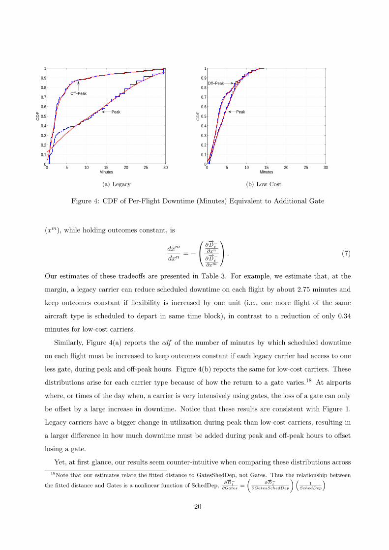
Figure 4: CDF of Per-Flight Downtime (Minutes) Equivalent to Additional Gate

(xm), while holding outcomes constant, is

dxm

dxn= −

∂−→D−

t∂xn

∂−→D−

t∂xm

. (7)

Our estimates of these tradeoffs are presented in Table 3. For example, we estimate that, at the

margin, a legacy carrier can reduce scheduled downtime on each flight by about 2.75 minutes and

keep outcomes constant if flexibility is increased by one unit (i.e., one more flight of the same

aircraft type is scheduled to depart in same time block), in contrast to a reduction of only 0.34

minutes for low-cost carriers.

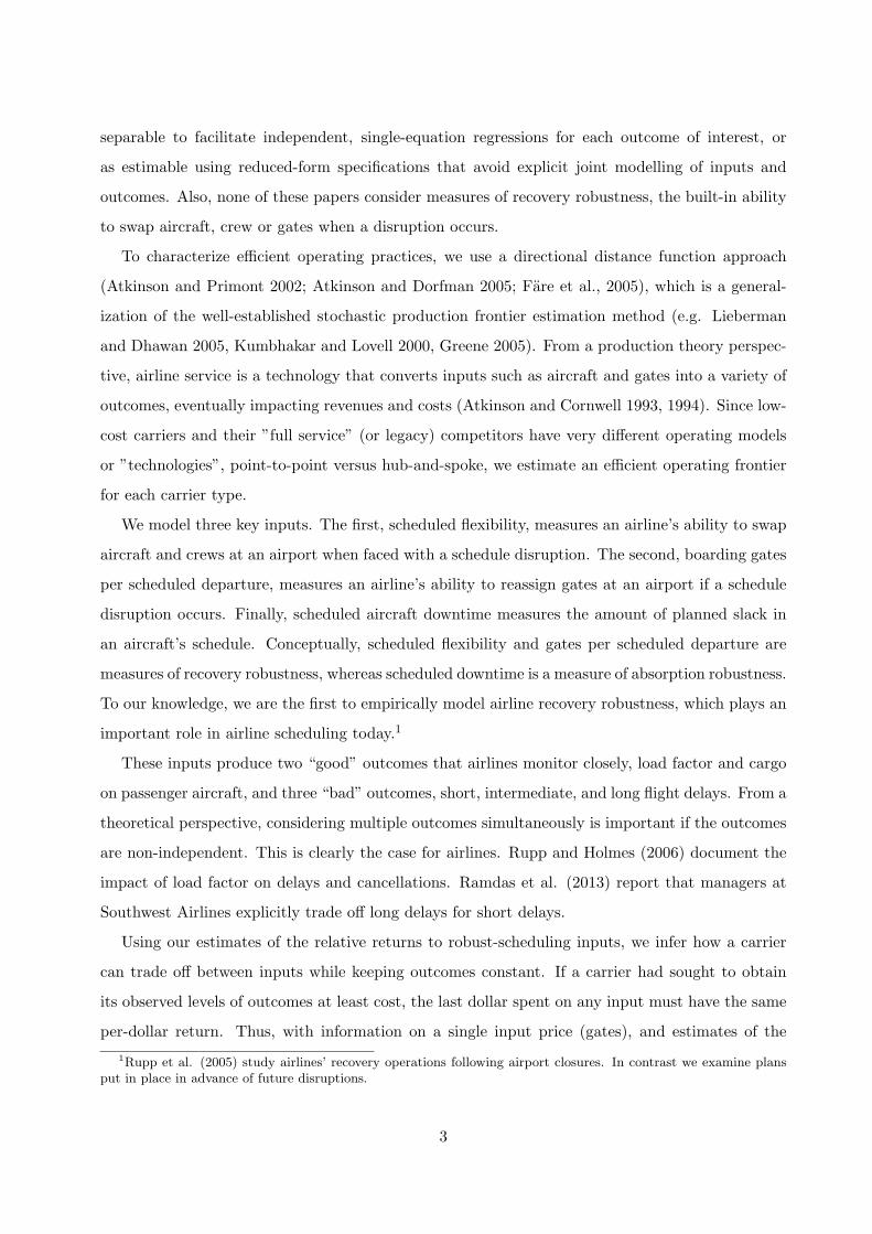
Similarly, Figure 4(a) reports the cdf of the number of minutes by which scheduled downtime

on each flight must be increased to keep outcomes constant if each legacy carrier had access to one

less gate, during peak and off-peak hours. Figure 4(b) reports the same for low-cost carriers. These

distributions arise for each carrier type because of how the return to a gate varies.18 At airports

where, or times of the day when, a carrier is very intensively using gates, the loss of a gate can only

be offset by a large increase in downtime. Notice that these results are consistent with Figure 1.

Legacy carriers have a bigger change in utilization during peak than low-cost carriers, resulting in

a larger difference in how much downtime must be added during peak and off-peak hours to offset

losing a gate.

Yet, at first glance, our results seem counter-intuitive when comparing these distributions across

18Note that our estimates relate the fitted distance to GatesShedDep, not Gates. Thus the relationship between

the fitted distance and Gates is a nonlinear function of SchedDep,∂−→D−

t∂Gates

=

(∂−→D−

t∂GatesSchedDep

)(1

SchedDep

)

20

0 5 10 15 20 25 300

0.1

0.2

0.3

0.4

0.5

0.6

0.7

0.8

0.9

1

Flights

CD

F

Off−Peak

Peak

(a) Legacy

0 5 10 15 20 25 30 35 400

0.1

0.2

0.3

0.4

0.5

0.6

0.7

0.8

0.9

1

Flights

CD

F Peak

Off−Peak

(b) Low Cost

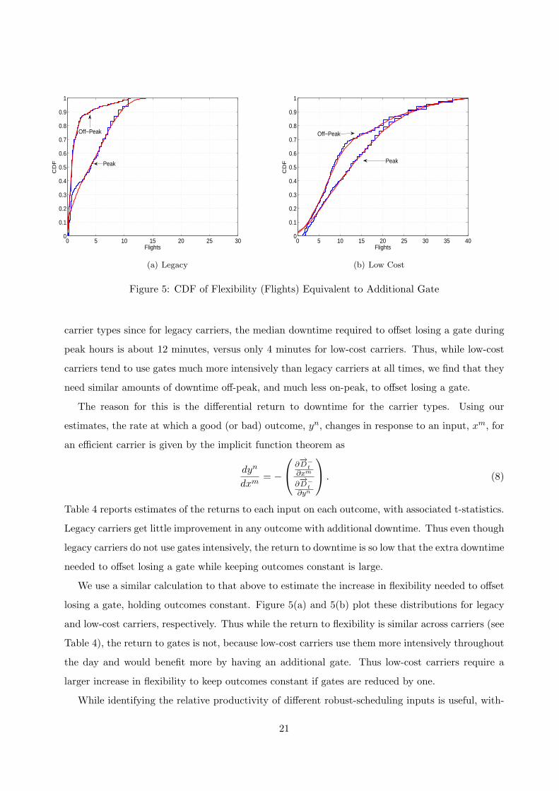
Figure 5: CDF of Flexibility (Flights) Equivalent to Additional Gate

carrier types since for legacy carriers, the median downtime required to offset losing a gate during

peak hours is about 12 minutes, versus only 4 minutes for low-cost carriers. Thus, while low-cost

carriers tend to use gates much more intensively than legacy carriers at all times, we find that they

need similar amounts of downtime off-peak, and much less on-peak, to offset losing a gate.

The reason for this is the differential return to downtime for the carrier types. Using our

estimates, the rate at which a good (or bad) outcome, yn, changes in response to an input, xm, for

an efficient carrier is given by the implicit function theorem as

dyn

dxm= −

∂−→D−

t∂xm

∂−→D−

t∂yn

. (8)

Table 4 reports estimates of the returns to each input on each outcome, with associated t-statistics.

Legacy carriers get little improvement in any outcome with additional downtime. Thus even though

legacy carriers do not use gates intensively, the return to downtime is so low that the extra downtime

needed to offset losing a gate while keeping outcomes constant is large.

We use a similar calculation to that above to estimate the increase in flexibility needed to offset

losing a gate, holding outcomes constant. Figure 5(a) and 5(b) plot these distributions for legacy

and low-cost carriers, respectively. Thus while the return to flexibility is similar across carriers (see

Table 4), the return to gates is not, because low-cost carriers use them more intensively throughout

the day and would benefit more by having an additional gate. Thus low-cost carriers require a

larger increase in flexibility to keep outcomes constant if gates are reduced by one.

While identifying the relative productivity of different robust-scheduling inputs is useful, with-

21

0 10 20 30 40 50 60 70 800

0.1

0.2

0.3

0.4

0.5

0.6

0.7

0.8

0.9

1

Dollars

CD

F

(a) Legacy

0 10 20 30 40 50 60 70 800

0.1

0.2

0.3

0.4

0.5

0.6

0.7

0.8

0.9

1

Dollars

CD

F

(b) Low Cost

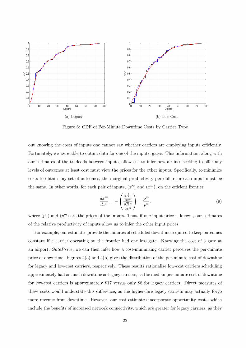
Figure 6: CDF of Per-Minute Downtime Costs by Carrier Type

out knowing the costs of inputs one cannot say whether carriers are employing inputs efficiently.

Fortunately, we were able to obtain data for one of the inputs, gates. This information, along with

our estimates of the tradeoffs between inputs, allows us to infer how airlines seeking to offer any

levels of outcomes at least cost must view the prices for the other inputs. Specifically, to minimize

costs to obtain any set of outcomes, the marginal productivity per dollar for each input must be

the same. In other words, for each pair of inputs, (xn) and (xm), on the efficient frontier

dxm

dxn= −

∂−→D−

t∂xn

∂−→D−

t∂xm

=pm

pn, (9)

where (pn) and (pm) are the prices of the inputs. Thus, if one input price is known, our estimates

of the relative productivity of inputs allow us to infer the other input prices.

For example, our estimates provide the minutes of scheduled downtime required to keep outcomes

constant if a carrier operating on the frontier had one less gate. Knowing the cost of a gate at

an airport, GatePrice, we can then infer how a cost-minimizing carrier perceives the per-minute

price of downtime. Figures 4(a) and 4(b) gives the distribution of the per-minute cost of downtime

for legacy and low-cost carriers, respectively. These results rationalize low-cost carriers scheduling

approximately half as much downtime as legacy carriers, as the median per-minute cost of downtime

for low-cost carriers is approximately $17 versus only $8 for legacy carriers. Direct measures of

these costs would understate this difference, as the higher-fare legacy carriers may actually forgo

more revenue from downtime. However, our cost estimates incorporate opportunity costs, which

include the benefits of increased network connectivity, which are greater for legacy carriers, as they

22

0 0.5 1 1.5 2 2.50

0.1

0.2

0.3

0.4

0.5

0.6

0.7

0.8

0.9

1

Dollars (1,000s)

CD

F

(a) Legacy

0 0.5 1 1.5 2 2.50

0.1

0.2

0.3

0.4

0.5

0.6

0.7

0.8

0.9

1

Dollars (1,000s)

CD

F

(b) Low Cost

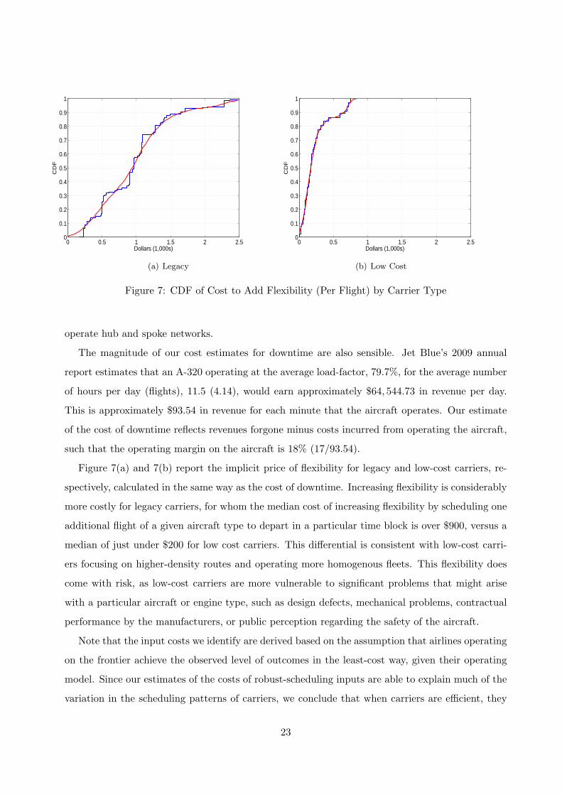
Figure 7: CDF of Cost to Add Flexibility (Per Flight) by Carrier Type

operate hub and spoke networks.

The magnitude of our cost estimates for downtime are also sensible. Jet Blue’s 2009 annual

report estimates that an A-320 operating at the average load-factor, 79.7%, for the average number

of hours per day (flights), 11.5 (4.14), would earn approximately $64, 544.73 in revenue per day.

This is approximately $93.54 in revenue for each minute that the aircraft operates. Our estimate

of the cost of downtime reflects revenues forgone minus costs incurred from operating the aircraft,

such that the operating margin on the aircraft is 18% (17/93.54).

Figure 7(a) and 7(b) report the implicit price of flexibility for legacy and low-cost carriers, re-

spectively, calculated in the same way as the cost of downtime. Increasing flexibility is considerably

more costly for legacy carriers, for whom the median cost of increasing flexibility by scheduling one

additional flight of a given aircraft type to depart in a particular time block is over $900, versus a

median of just under $200 for low cost carriers. This differential is consistent with low-cost carri-

ers focusing on higher-density routes and operating more homogenous fleets. This flexibility does

come with risk, as low-cost carriers are more vulnerable to significant problems that might arise

with a particular aircraft or engine type, such as design defects, mechanical problems, contractual

performance by the manufacturers, or public perception regarding the safety of the aircraft.

Note that the input costs we identify are derived based on the assumption that airlines operating

on the frontier achieve the observed level of outcomes in the least-cost way, given their operating

model. Since our estimates of the costs of robust-scheduling inputs are able to explain much of the

variation in the scheduling patterns of carriers, we conclude that when carriers are efficient, they

23

appear to be selecting the least-cost means of producing outcomes.

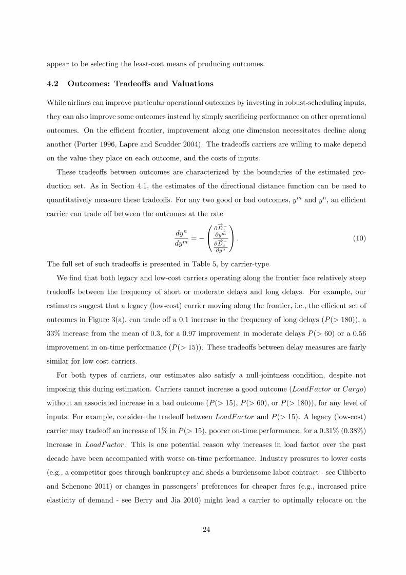
4.2 Outcomes: Tradeoffs and Valuations

While airlines can improve particular operational outcomes by investing in robust-scheduling inputs,

they can also improve some outcomes instead by simply sacrificing performance on other operational

outcomes. On the efficient frontier, improvement along one dimension necessitates decline along

another (Porter 1996, Lapre and Scudder 2004). The tradeoffs carriers are willing to make depend

on the value they place on each outcome, and the costs of inputs.

These tradeoffs between outcomes are characterized by the boundaries of the estimated pro-

duction set. As in Section 4.1, the estimates of the directional distance function can be used to

quantitatively measure these tradeoffs. For any two good or bad outcomes, ym and yn, an efficient

carrier can trade off between the outcomes at the rate

dyn

dym= −

∂−→D−

t∂ym

∂−→D−

t∂yn

. (10)

The full set of such tradeoffs is presented in Table 5, by carrier-type.

We find that both legacy and low-cost carriers operating along the frontier face relatively steep

tradeoffs between the frequency of short or moderate delays and long delays. For example, our

estimates suggest that a legacy (low-cost) carrier moving along the frontier, i.e., the efficient set of

outcomes in Figure 3(a), can trade off a 0.1 increase in the frequency of long delays (P (> 180)), a

33% increase from the mean of 0.3, for a 0.97 improvement in moderate delays P (> 60) or a 0.56

improvement in on-time performance (P (> 15)). These tradeoffs between delay measures are fairly

similar for low-cost carriers.

For both types of carriers, our estimates also satisfy a null-jointness condition, despite not

imposing this during estimation. Carriers cannot increase a good outcome (LoadFactor or Cargo)

without an associated increase in a bad outcome (P (> 15), P (> 60), or P (> 180)), for any level of

inputs. For example, consider the tradeoff between LoadFactor and P (> 15). A legacy (low-cost)

carrier may tradeoff an increase of 1% in P (> 15), poorer on-time performance, for a 0.31% (0.38%)

increase in LoadFactor. This is one potential reason why increases in load factor over the past

decade have been accompanied with worse on-time performance. Industry pressures to lower costs

(e.g., a competitor goes through bankruptcy and sheds a burdensome labor contract - see Ciliberto

and Schenone 2011) or changes in passengers’ preferences for cheaper fares (e.g., increased price

elasticity of demand - see Berry and Jia 2010) might lead a carrier to optimally relocate on the

24

frontier (i.e., maintain allocative efficiency as prices of outcomes evolve), raising load factors to

lower costs, while accepting poorer on-time performance.

Since we have estimates of these tradeoffs between outcomes, based on where carriers have

chosen to locate on the frontier, we are able to say something about how carriers view the relative

prices of the outcomes. For example, we estimate that at the margin, a low-cost (legacy) carrier

is willing to tradeoff a 0.1% increase in P (> 180) for a 0.56% (0.42%) decrease in P (> 15). Thus,

low-cost and legacy carriers view long delays as approximately 4 and 5 times, respectively, more

costly than poor on-time performance, consistent with the results of Ramdas et. al (2012).

Similarly, low-cost (legacy) carriers are willing to accept a 1% increase in P (> 15) for a 0.38%

(0.31%) increase in LoadFactor. Consider again the numbers from JetBlue’s 2009 annual report.

JetBlue chose to operate their A-320 aircraft, with seating capacity of 150, at an average load-factor

of 79.7%, i.e. at an average of 119.55 passengers on each flight. Thus, JetBlue chose to forgo a

0.38% increase in load-factor (0.57 passengers on average) to increase the probability that its flights

were on time (no greater than 15 minutes late) by 1%. JetBlue estimates that the average one-way

fare was $130.41. Thus JetBlue sacrificed $74.33 (130.41*0.57) to ensure that on-time performance

increased by 1%. In 2009, JetBlue was on-time 77.5% of the time, late 22.5%. JetBlue operated

16,774 flights in December 2009. Thus to improve on-time performance in its network during this

month by 1%, or lower the level by 4.44% (1/22.5), it cost JetBlue $1, 246, 811.42 (16,774*74.33)

in forgone revenues. A similar exercise can be done for other outcomes using the forgone revenue

resulting from sacrificed improvements in load-factor.

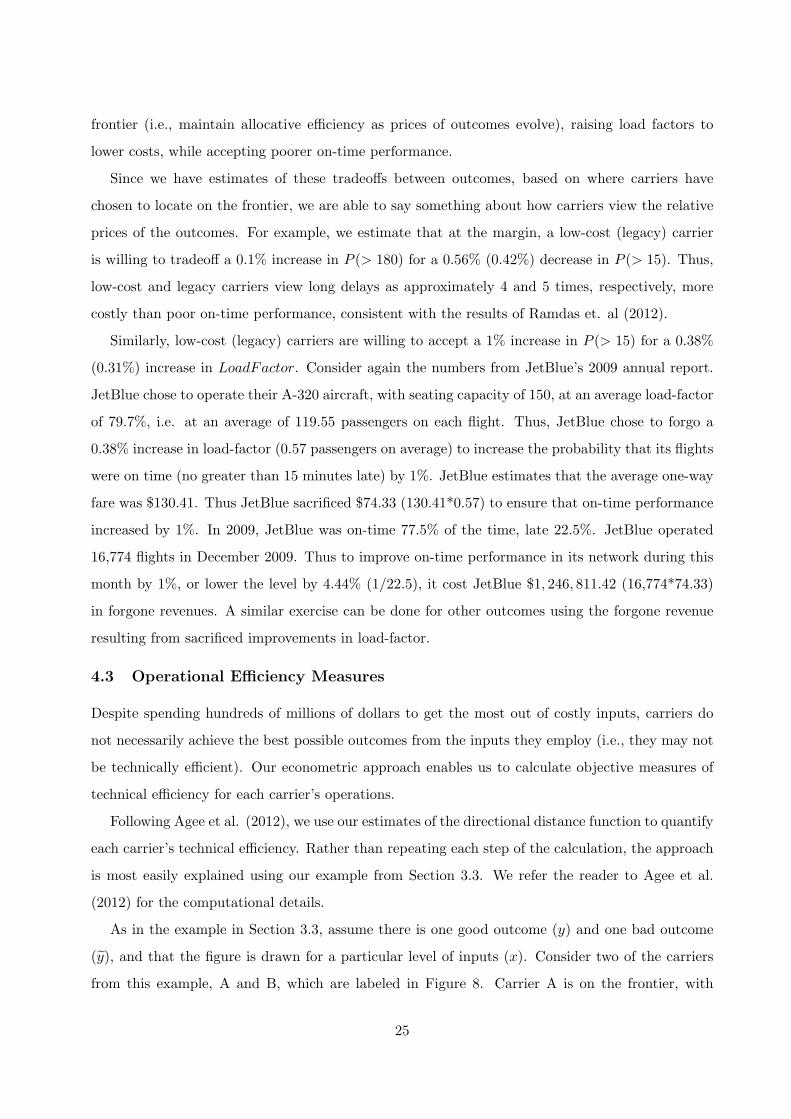
4.3 Operational Efficiency Measures

Despite spending hundreds of millions of dollars to get the most out of costly inputs, carriers do

not necessarily achieve the best possible outcomes from the inputs they employ (i.e., they may not

be technically efficient). Our econometric approach enables us to calculate objective measures of

technical efficiency for each carrier’s operations.

Following Agee et al. (2012), we use our estimates of the directional distance function to quantify

each carrier’s technical efficiency. Rather than repeating each step of the calculation, the approach

is most easily explained using our example from Section 3.3. We refer the reader to Agee et al.

(2012) for the computational details.

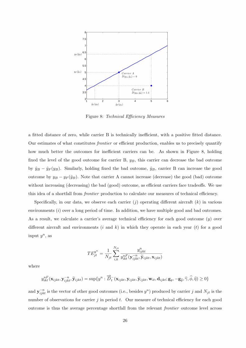
As in the example in Section 3.3, assume there is one good outcome (y) and one bad outcome

(y), and that the figure is drawn for a particular level of inputs (x). Consider two of the carriers

from this example, A and B, which are labeled in Figure 8. Carrier A is on the frontier, with

25

1 2 3 4 5 63

3.5

4

4.5

5

5.5

6

6.5

7

7.5

8

Carrier A

D(yA, yA) = 0

Carrier B

D(yB , yB) = 1.4

yF (yB)

yF (yA)

yF (yB) yF (yA)

Figure 8: Technical Efficiency Measures

a fitted distance of zero, while carrier B is technically inefficient, with a positive fitted distance.

Our estimates of what constitutes frontier or efficient production, enables us to precisely quantify

how much better the outcomes for inefficient carriers can be. As shown in Figure 8, holding

fixed the level of the good outcome for carrier B, yB, this carrier can decrease the bad outcome

by yB − yF (yB). Similarly, holding fixed the bad outcome, yB, carrier B can increase the good

outcome by yB − yF (yB). Note that carrier A cannot increase (decrease) the good (bad) outcome

without increasing (decreasing) the bad (good) outcome, as efficient carriers face tradeoffs. We use

this idea of a shortfall from frontier production to calculate our measures of technical efficiency.

Specifically, in our data, we observe each carrier (j) operating different aircraft (k) in various

environments (i) over a long period of time. In addition, we have multiple good and bad outcomes.

As a result, we calculate a carrier’s average technical efficiency for each good outcome (y) over

different aircraft and environments (i and k) in which they operate in each year (t) for a good

input yn, as

TEyn

jt =1

Njt

Njt∑i,k

ynijkt

ynFikt (y−nijkt, yijkt,xijkt)

where

ynFikt (xijkt,y−nijkt, yijkt) = sup{yn :

−→D−

t (xijkt,yijkt, yijkt,wit,dijkt;gy,−gy, γ, ϕ, η) ≥ 0}

and y−nijkt is the vector of other good outcomes (i.e., besides yn) produced by carrier j and Njt is the

number of observations for carrier j in period t. Our measure of technical efficiency for each good

outcome is thus the average percentage shortfall from the relevant frontier outcome level across

26

those environments in which the carrier operates in period t. Similarly, for a bad outcome, yn, we

measure each carrier’s operational efficiency as

TE yn

jt = 1− 1

Njt

Njt∑i,k

[ynijkt − ynFikt (yijkt, y

−nijkt,xijkt)

]where

ynFikt (yijkt, y−nijkt,xijkt) = inf{yn :

−→D−

t (xijkt,yijkt, yijkt,wit,dijkt;gy,−gy, γ, ϕ, η) ≥ 0}

and y−nijkt is the vector of other bad outcomes (i.e., besides yn) produced by carrier j.

The reason for taking the absolute difference of a carrier’s outcome and the frontier outcome

level in the case of bad outcomes (i.e., our delays measures) is that the frontier firm might have

zero delays so that a relative measure would not be well-defined. Thus, our measure of a carrier’s

efficiency with respect to each of the bad outcomes is the reduction in the bad outcome that would

be required to reach the frontier, holding constant inputs and other outcomes. This bounds our

measures of technical efficiency for both good and bad outcomes between zero and one.

Note that our measures of efficiency credit carriers for operating in more difficult environments

by normalizing their outcome levels by the frontier outcome level in each environment. In difficult

environments, the frontier outcome level is characterized by higher levels of bad outcomes and

lower levels of good outcomes. Thus, a carrier’s performance relative to the best practices in each

environment is captured by our measures.

The estimates of carriers’ relative efficiency in 2007 are presented in Table 5.19 For both good

and bad outcomes, the relative measures are bounded between 0 and 1, with the most efficient

firm having a value of 1. For example, Delta’s relative measure of 0.91 for LoadFactor (a good

outcome) implies that, after conditioning on levels of inputs and other outcomes, Delta achieves

91% of the frontier level of LoadFactor defined as 1.0 by American. Similarly, Delta’s measure of

0.98 for P (> 180) (a bad outcome) implies that Delta would need to reduce the frequency of long

delays by 0.02, holding the level of inputs and other outcomes constant, to reach the frontier.

The efficiency measures for the bad outcomes in Table 5 are interesting. Northwest is the

most efficient carrier for each of the delay measures; however, Continental is a very close second.

This result is completely counter to Table 1 if one considers the delay measures in isolation, as

19It is not possible to compare all 10 carriers in the earlier years, 1997 and 2001, as some of the low-cost carrierswere not yet large enough (1% of domestic enplanements) to be required to report operating data to the DOT. Wereport efficiency results for 2007 because the gate survey had the highest response rate in this year. Results in 2008and 2009 are very similar.

27

Continental performs rather poorly across each measure of delays. This result can be rationalized

by the input decisions in the bottom half of Table 1. Continental employs much smaller amounts of

Downtime and Flex than other legacy carriers, and is very near the top in terms of gate utilization.

This example makes clear how our approach explicitly credits carriers for increasing good outcomes

and reducing bad outcomes for a given level of inputs. American’s last-place ranking for each of

the bad outcomes can be explained by its high frequency of each type of delay along with the large

amount of inputs that American employs.

Our estimates of carriers’ technical efficiency can be used to quantify the revenue that the carrier

would have realized, if not for the inefficiencies. For example, across JetBlue’s network loadfactor

was 79.7% in 2009; however, we estimate that this was only 89% of the maximum achievable load

factor given the level of JetBlue’s other outcomes (delays and cargo). JetBlue is one of the worst

in terms of on-time performance in 2009, late 22.5% of the time. Our estimates suggest that an

efficient carrier that chose such poor on-time performance could have achieved a load factor of

approximately 89%. Thus JetBlue’s inefficiencies cost them approximately 14.78 passengers per

flight, at the average fare of $130.41; this corresponds to $1926.80 per flight, or 3% of per-flight

revenues ($64, 544.73). Identifying these sources of this inefficiency (e.g., management, local airport

operations, etc) is a high priority for future research.

Southwest’s ranking is also of particular interest, as it is often touted as a successful operating

model for the industry. Our results suggest that once input choices and environmental factors are

controlled for, any ”Southwest effect” is largely explained away. Essentially, Southwest’s operational

outcomes are about average if one conditions on the level of inputs employed and compares carriers

in similar operating environments.

5 Concluding Remarks

We characterize efficient operating practices in the airline industry with respect to robust scheduling

practices by estimating a multiple-outcome, multiple-input production frontier. We use estimates

of the returns to robust scheduling inputs, which indicate the tradeoffs faced by carriers along this

frontier, to infer how carriers view the costs of robust-scheduling inputs and the value they place

on various operational outcomes. We also measure the costs of technical inefficiencies in carriers’

networks.

In doing so, we make several contributions. To our knowledge, we are the first to empirically

model recovery robustness, which is a vital ingredient of air carriers’ robust scheduling practices.

28

We measure the returns (i.e., improvement in operational outcomes) and costs associated with two

forms of recovery robustness (flexibility to swap aircraft and crew, and flexibility to swap gates) and

one form of absorption robustness (downtime). Prior OR research modeling schedule robustness

highlights the difficulty in estimating these costs, since they are less-clearly-defined opportunity

costs in the form of forgone revenue (Smith and Johnson 2006). These cost estimates rationalize

the different scheduling practices used by legacy and low-cost carriers. Second, we estimate the

value that carriers place on certain outcomes. For example, we estimate that JetBlue values a 1%

increase in the probability that a flight is on time at $74.33. Finally, we quantify the significant

revenue that carriers lose due to operations that are technically inefficient. We estimate that given

its high level of delays, JetBlue only achieves 89% of the efficient loadfactor. This inefficiency costs

JetBlue $1926.80 per flight in lost revenues.

Our estimates of the costs of robust scheduling inputs and the value placed on operational

outcomes are useful to both managers and policy makers. Managers can use our cost estimates

to identify ways to change their input mix so as to reduce their costs of achieving their desired

levels of operational outcomes, and to estimate the resulting cost savings. Similarly, managers

can compare our estimates of the valuation they place on operational outcomes to decide whether

relocating on the frontier will improve profitability. Finally, managers can use our estimates of

technical efficiency to determine how far an airline is from the efficient frontier in very specific

environments. By utilizing estimates of environment-specific inefficiencies, along with detailed

proprietary information on local operations, managers can uncover the source of the inefficiencies

and remove them. Industry regulators and policy makers can use our estimates to identify the

most efficient way to enact policies that improve industry performance and enhance the welfare

of passengers, as directed by the FAA Modernization and Reform Act of 2012. This includes

weighing the costs to carriers from reducing delays against the costs associated with alternatives

like expanding airport facilties to alleviate congestion.

Both our application and methodology provide direction for future research. Our applica-

tion demonstrates the importance of accounting for recovery robustness when examining airlines’

scheduling practices. We show that there are significant returns to recovery robustness, which

suggests the need for OR researchers to develop models that formally account for it. While some

progress has been made (Clausen et al., 2010), further work needs to be done. In terms of method-

ology, we adapt econometric tools recently developed in the economics literature (Atkinson and

Primont 2002, Atkinson and Dorfman 2005, and Fare et al. 2005) to study scheduling practices in

an extremely complex operating environment. The flexibility of these tools make them amenable

29

to identifying efficient operating practices in important industries like health care, education, and

utilities.

References

[1] Agee, M., S. Atkinson, and T. Crocker. 2012. Child Maturation, Time-Invariant, and Time-Varying Inputs; Their Interaction in the Production of Child Human Capital. Journal ofProductivity Analysis. 38 29-44.

[2] Arguello, M., J. Bard and G. Yu. 1997. A GRASP for Aircraft Routing in Response to Ground-ings and Delays. Journal of Combinatorial Optimization. 5 211-228.

[3] Arikan, M., V. Deshpande, and M. Sohoni. 2012. Building Reliable Air-Travel InfrastructureUsing Empirical Data and Stochastic Models of Airline Networks. Working paper.

[4] Atkinson, S. and C. Cornwell. 1993. Measuring Technical Efficiency with Panel Data: A DualApproach. Journal of Econometrics. 59 257-261.

[5] Atkinson, S. and C. Cornwell. 1994. Parametric Estimation of Technical and Allocative Inef-ficiency with Panel Data. International Economic Review. 35 231-243.

[6] Atkinson, S. and D. Primont. 2002. Stochastic Estimation of Firm Technology, Inefficiency, andProductivity Growth Using Shadow Cost and Distance Functions. Journal of Econometrics.108(2) 203-225.

[7] Atkinson, S. and J. Dorfman. 2005. Bayesian Measurement of Productivity and Efficiency inthe Presence of Undesirable Outputs: Crediting Electric Utilities for Reducing Air Pollution.Journal of Econometrics. 126(2) 445-468.

[8] Berndt, E. and D. Wood. 1975. Technology, Prices, and the Derived Demand for Energy. TheReview of Economics and Statistics. 57(3) 259-268.

[9] Berry, S. and P. Jia. 2010. Tracing the Woes: An Empirical Analysis of the Airline Industry.American Economic Journal: Microeconomics. 2(3) 1-43.

[10] Brueckner, J. 2002. Airport Congestion When Carriers Have Market Power. American Eco-nomic Review. 92(5) 1357-1375.

[11] Brueckner, J. 2005. Internalization of Airport Congestion: A Network Analysis. InternationalJournal of Industrial Organization. 23(7-8) 599-614.

[12] Cannon, J., T. Randall, and C. Terwiesch. 2012. An Operations Based Earnings PredictionModel Applied to the US Airline Industry. Working Paper.

[13] Chambers, R., Y. Chung, and R. Fare. 1998. Profit, Directional Distance Functions, andNerlovian Efficiency. Journal of Optimization Theory and Applications. 98(2) 351-364.

[14] Ciliberto, F. and C. Schenone. 2011. Bankruptcy and Product-Market Competition in theAirline Industry. International Journal of Industrial Organization, Forthcoming.

[15] Ciliberto, F. and J. Williams. 2010. Limited Access to Airport Facilities and Market Powerin the Airline Industry. Journal of Law and Economics. 53(2) 467-495.

[16] Clausen, J., A. Larsen, J. Larsen, and N. Rezanova. 2010. Disruption Management in theAirline Industry - Concepts, Models and Methods. Computers & Operations Research. 37809-821.

[17] Daniel, J.. 1995. Congestion Pricing and Capacity of Large Hub Airports: A Bottleneck Modelwith Stochastic Queues. Econometrica. 63(2) 327-370.

30

[18] Deshpande, V. and M. Arikan. 2011. The Impact of Airline Flight Schedules on Flight Delays.Manufacturing & Service Operations Management, Forthcoming.

[19] Fare, R., S. Grosskopf, D. Noh, and W. Weber. 2005. Characteristics of a Polluting Technology:Theory and Practice. Journal of Econometrics. 126(2) 469-492.

[20] Greene, W. 2005. Reconsidering Heterogeneity in Panel Data Estimators of the StochasticFrontier Model. Journal of Econometrics. 126(2) 269-303.

[21] Kumbhakar, S. and C. Lovell. 2000. Stochastic Frontier Analysis. Cambridge University Press.

[22] Lan, S., J.P. Clarke, and C. Barnhart. 2006. Planning for Robust Airline Operations: Op-timizing Aircraft Routings and Flight Departure Times to Minimize Passenger Disruptions.Transportation Science. 40 15-28.

[23] Lapre, M. and G. Scudder. 2004. Performance Improvement Paths in the U.S. Airline Industry:Linking Tradeoffs to Asset Frontiers. Production and Operations Management. 13(2) 123–134.

[24] Lieberman, M. and R. Dhawan. 2005. Assessing the Resource Base of Japanese and U.S. AutoProducers: A Stochastic Frontier Production Approach. Management Science. 51(7) 1060-1075.

[25] Mayer, C. and T. Sinai. 2003. Network Effects, Congestion Externalities, and Air Traffic Delays:Or Why All Delays Are Not Evil. American Economic Review. 93(4) 1194-1215.

[26] Mazzeo, M. 2003. Competition and Service Quality in the US Airline Industry. Review ofIndustrial Organization. 22 275–296.

[27] Li, J. and S. Netessine. 2011. Partnering with Competitors – An Empirical Analysis of AirlineAlliances and Multimarket Competition. SSRN Working Paper 1761211.

[28] Olivares, M., C. Terwiesch, and L. Cassorla. 2008. Structural Estimation of the NewsvendorModel: An Application to Reserving Operating Room Time. Management Science. 54 41-55.

[29] Porter, M. 1996. What Is Strategy? Harvard Business Review. Nov.-Dec. 6-78.

[30] Ramdas, K., J. Williams and M. Lipson. 2013. Can Stock Price Movements Inform Opera-tional Improvement Efforts? Evidence from the Airline Industry. Manufacturing & ServiceOperations Management, Forthcoming.

[31] Rosenberger, J., A. Schaefer, D. Goldsman, E. Johnson, A. Kleywegt, and G. Nemhauser.2002. A Stochastic Model of Airline Operations. Transportation Science. 36 357-377.

[32] Rupp, N. 2009. Do Carriers Internalize Congestion Costs? Empirical Evidence on the Inter-nalization Question. Journal of Urban Economics. 65(1) 24-37.

[33] Rupp, N. and G. Holmes. 2006. An Investigation into the Determinants of Flight Cancellations.Economica. 73(292) 749-783.

[34] Rupp, N., G. Holmes, and J. DeSimone. 2005. Airline Schedule Recovery after Airport Clo-sures: Empirical Evidence since September 11. Southern Economic Journal. 71(4) 800-820.

[35] Shumsky, R. 1993. Response of U.S. Air Carriers to On-Time Disclosure Rule. TransportationResearch Record. 1379 9-16.

[36] Smith, B. and E. Johnson. 2006. Robust Airline Fleet Assignment: Imposing Station PurityUsing Station Decomposition. Transportation Science. 40(4) 497-516.

[37] Snider, C. and J. Williams. 2012. Barriers to Entry in the Airline Industry: A Multi-Dimensional Regression-Discontinuity Analysis of the Wendell H. Ford Aviation Investmentand Reform Act. Working Paper.

[38] Williams, J. 2012. Capacity Investments, Exclusionary Behavior, and Welfare: A DynamicModel of Competition in the Airline Industry. Working Paper.

31

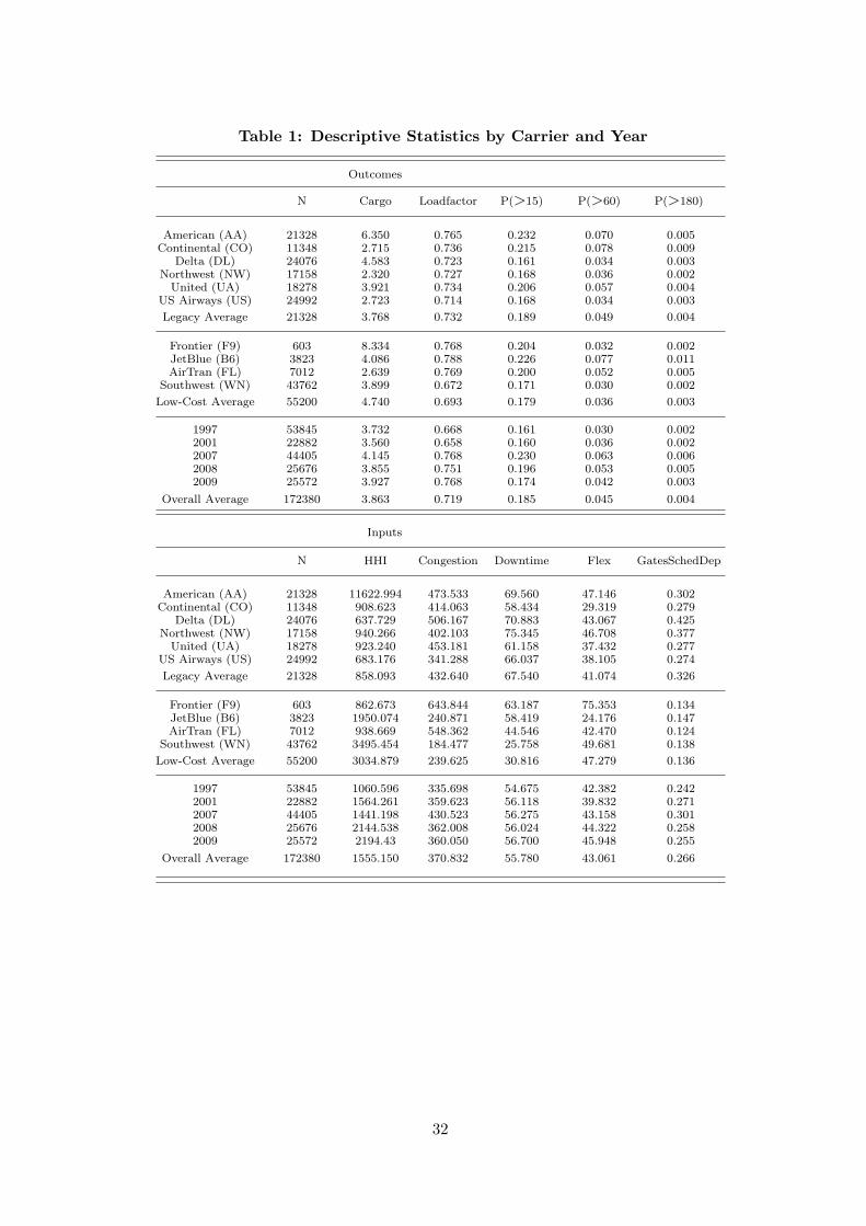
Table 1: Descriptive Statistics by Carrier and Year

Outcomes

N Cargo Loadfactor P(>15) P(>60) P(>180)

American (AA) 21328 6.350 0.765 0.232 0.070 0.005Continental (CO) 11348 2.715 0.736 0.215 0.078 0.009

Delta (DL) 24076 4.583 0.723 0.161 0.034 0.003Northwest (NW) 17158 2.320 0.727 0.168 0.036 0.002United (UA) 18278 3.921 0.734 0.206 0.057 0.004

US Airways (US) 24992 2.723 0.714 0.168 0.034 0.003

Legacy Average 21328 3.768 0.732 0.189 0.049 0.004

Frontier (F9) 603 8.334 0.768 0.204 0.032 0.002JetBlue (B6) 3823 4.086 0.788 0.226 0.077 0.011AirTran (FL) 7012 2.639 0.769 0.200 0.052 0.005

Southwest (WN) 43762 3.899 0.672 0.171 0.030 0.002

Low-Cost Average 55200 4.740 0.693 0.179 0.036 0.003

1997 53845 3.732 0.668 0.161 0.030 0.0022001 22882 3.560 0.658 0.160 0.036 0.0022007 44405 4.145 0.768 0.230 0.063 0.0062008 25676 3.855 0.751 0.196 0.053 0.0052009 25572 3.927 0.768 0.174 0.042 0.003

Overall Average 172380 3.863 0.719 0.185 0.045 0.004

Inputs

N HHI Congestion Downtime Flex GatesSchedDep

American (AA) 21328 11622.994 473.533 69.560 47.146 0.302Continental (CO) 11348 908.623 414.063 58.434 29.319 0.279

Delta (DL) 24076 637.729 506.167 70.883 43.067 0.425Northwest (NW) 17158 940.266 402.103 75.345 46.708 0.377United (UA) 18278 923.240 453.181 61.158 37.432 0.277

US Airways (US) 24992 683.176 341.288 66.037 38.105 0.274

Legacy Average 21328 858.093 432.640 67.540 41.074 0.326

Frontier (F9) 603 862.673 643.844 63.187 75.353 0.134JetBlue (B6) 3823 1950.074 240.871 58.419 24.176 0.147AirTran (FL) 7012 938.669 548.362 44.546 42.470 0.124

Southwest (WN) 43762 3495.454 184.477 25.758 49.681 0.138

Low-Cost Average 55200 3034.879 239.625 30.816 47.279 0.136

1997 53845 1060.596 335.698 54.675 42.382 0.2422001 22882 1564.261 359.623 56.118 39.832 0.2712007 44405 1441.198 430.523 56.275 43.158 0.3012008 25676 2144.538 362.008 56.024 44.322 0.2582009 25572 2194.43 360.050 56.700 45.948 0.255

Overall Average 172380 1555.150 370.832 55.780 43.061 0.266

32

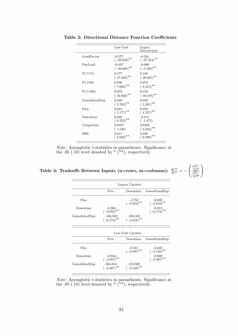
Table 2: Directional Distance Function Coefficients

Low-Cost LegacyInteractions

LoadFactor -0.277 -0.501( -49.833)∗∗ ( -37.354)∗∗

PayLoad -0.437 -0.090

( -46.005)∗∗ ( -5.520)∗∗

P(>15) 0.177 0.186

( 47.403)∗∗ ( 28.265)∗∗

P(>60) 0.030 0.072

( 7.669)∗∗ ( 9.415)∗∗

P(>180) 0.078 0.152

( 16.928)∗∗ ( 16.478)∗∗

GatesSchedDep 0.029 0.029

( 5.763)∗∗ ( 3.381)∗∗

Flex 0.043 0.058( 5.177)∗∗ ( 4.237)∗∗

Downtime 0.042 -0.015( 6.252)∗∗ ( -1.475)

Congestion 0.0167 0.0458

( 1.536) ( 2.835)∗∗

HHI 0.017 0.059( 2.683)∗∗ ( 6.290)∗∗

Note: Asymptotic t-statistics in parantheses. Significance atthe .05 (.10) level denoted by * (**), respectively.

Table 3: Tradeoffs Between Inputs (n=rows, m=columns): dxm

dxn = −

(∂−→D−

t∂xn

∂−→D−

t∂xm

)

Legacy Carriers

Flex Downtime GatesSchedDep

Flex -2.752 -0.002( -3.053)∗∗ ( -2.918)∗∗

Downtime -0.363 -0.013( -3.053)∗∗ ( -6.174)∗∗

GatesSchedDep -106.923 -294.231

( -6.174)∗∗ ( -2.918)∗∗

Low Cost Carriers

Flex Downtime GatesSchedDep

Flex -0.341 -0.003( -4.097)∗∗ ( -4.128)∗∗

Downtime -2.934 -0.008( -4.097)∗∗ ( -4.367)∗∗

GatesSchedDep -363.654 -123.929

( -4.367)∗∗ ( -4.128)∗∗

Note: Asymptotic t-statistics in parantheses. Significance atthe .05 (.10) level denoted by * (**), respectively.

33

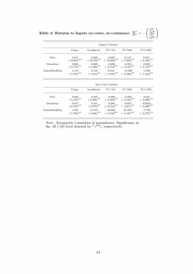
Table 4: Returns to Inputs (n=rows, m=columns): dym

dxn = −

(∂−→D−

t∂xn

∂−→D−

t∂ym

)

Legacy Carriers

Cargo Loadfactor P(>15) P(>60) P(>180)

Flex 0.011 0.026 -0.083 -0.145 -0.015( 10.657)∗∗ ( 10.502)∗∗ ( -10.800)∗∗ ( -7.059)∗∗ ( -9.492)∗∗

Downtime 0.004 0.009 -0.030 -0.053 -0.005( 3.172)∗∗ ( 3.190)∗∗ ( -3.173)∗∗ ( -3.125)∗∗ ( -3.137)∗∗

GatesSchedDep 1.141 2.743 -8.841 -15.502 -1.592

( 7.873)∗∗ ( 7.912)∗∗ ( -7.876)∗∗ ( -7.030)∗∗ ( -7.313)∗∗

Low Cost Carriers

Cargo Loadfactor P(>15) P(>60) P(>180)

Flex 0.005 0.035 -0.090 -0.223 -0.021( 5.176)∗∗ ( 4.996)∗∗ ( -5.076)∗∗ ( -4.245)∗∗ ( -4.806)∗∗

Downtime 0.015 0.101 -0.263 -0.654 -0.0624( 6.252)∗∗ ( 6.070)∗∗ ( -6.154)∗∗ ( -4.651)∗∗ ( -5.486)∗∗

GatesSchedDep 1.848 12.572 -32.626 -81.019 -7.726

( 5.763)∗∗ ( 5.668)∗∗ ( -5.748)∗∗ ( -4.547)∗∗ ( -5.278)∗∗

Note: Asymptotic t-statistics in parantheses. Significance atthe .05 (.10) level denoted by * (**), respectively.

34

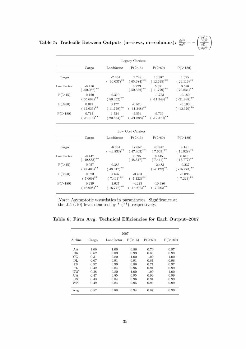
Table 5: Tradeoffs Between Outputs (n=rows, m=columns): dym

dyn = −

(∂−→D−

t∂yn

∂−→D−

t∂ym

)

Legacy Carriers

Cargo Loadfactor P(>15) P(>60) P(>180)

Cargo -2.404 7.749 13.587 1.395

( -60.037)∗∗ ( 65.684)∗∗ ( 12.635)∗∗ ( 26.116)∗∗

Loadfactor -0.416 3.223 5.651 0.580( -60.037)∗∗ ( 50.352)∗∗ ( 11.729)∗∗ ( 20.834)∗∗

P(>15) 0.129 0.310 -1.753 -0.180

( 65.684)∗∗ ( 50.352)∗∗ ( -11.348)∗∗ ( -21.888)∗∗

P(>60) 0.074 0.177 -0.570 -0.103

( 12.635)∗∗ ( 11.729)∗∗ ( -11.348)∗∗ ( -12.370)∗∗

P(>180) 0.717 1.724 -5.554 -9.739

( 26.116)∗∗ ( 20.834)∗∗ ( -21.888)∗∗ ( -12.370)∗∗

Low Cost Carriers

Cargo Loadfactor P(>15) P(>60) P(>180)

Cargo -6.804 17.657 43.847 4.181

( -49.833)∗∗ ( 47.403)∗∗ ( 7.669)∗∗ ( 16.928)∗∗

Loadfactor -0.147 2.595 6.445 0.615( -49.833)∗∗ ( 48.317)∗∗ ( 7.441)∗∗ ( 16.777)∗∗

P(>15) 0.057 0.385 -2.483 -0.237

( 47.403)∗∗ ( 48.317)∗∗ ( -7.122)∗∗ ( -15.273)∗∗

P(>60) 0.023 0.155 -0.403 -0.095

( 7.669)∗∗ ( 7.441)∗∗ ( -7.122)∗∗ ( -7.223)∗∗

P(>180) 0.239 1.627 -4.223 -10.486

( 16.928)∗∗ ( 16.777)∗∗ ( -15.273)∗∗ ( -7.223)∗∗

Note: Asymptotic t-statistics in parantheses. Significance atthe .05 (.10) level denoted by * (**), respectively.

Table 6: Firm Avg. Technical Efficiencies for Each Output–2007

2007

Airline Cargo Loadfactor P(>15) P(>60) P(>180)

AA 1.00 1.00 0.86 0.70 0.97B6 0.62 0.89 0.93 0.85 0.98CO 0.31 0.80 1.00 1.00 1.00DL 0.67 0.91 0.91 0.81 0.98F9 0.97 0.99 0.86 0.71 0.97FL 0.42 0.84 0.96 0.91 0.99NW 0.28 0.80 1.00 1.00 1.00UA 0.47 0.85 0.95 0.90 0.99US 0.43 0.84 0.96 0.91 0.99WN 0.49 0.84 0.95 0.90 0.99

Avg. 0.57 0.88 0.94 0.87 0.99

35