Embed Size (px)
Citation preview

ARTIKLER FRA STATISTISK SENTRALBYRÅ NR. 121
ON THE CAUSES AND EFFECTSOF NON-RESPONSE.
NORWEGIAN EXPERIENCES
By/Av Ib Thomsen and Erling Siring
OM ÅRSAKENE TIL OG VIRKNINGENEAV FRAFALL.
ERFARINGER FRA NORGE
OSLO 1980
ISBN 82-537-1107-7ISSN 0085-431x

PREFACE
During the last ten years non-response has grown into one of the
most serious problems in survey work. This article describes the work
done by the Central Bureau of Statistics of Norway to gain insight into
the effects of non-response, and the efforts made to keep response rates
at maximal level through effective operational procedures.
The paper was written at the invitation of National Research
Council in USA.
Central Bureau of Statistics, Oslo, 11 March 1980
Petter Jakob Bjerve
FORORD
Gjennom de siste ti år har frafall i Byråets utvalgsundersOkelser
blitt et stadig større problem. Denne artikkelen beskriver hva som er
gjort for å få innsikt i virkningene av frafall, og redusere frafallet
til et minimum.
Artikkelen er på engelsk, fordi den ble skrevet på anmodning av
National Research Council i USA.
Statistisk Sentralbyrå, Oslo, 11. mars 1980
Petter Jakob Bjerve

CONTENTS
Page
1. Introduction 7
2. Declining response rates 8
3. Factors affecting non-response 12
3.1. Strategy for the analysis of non-response data 12
3.2. Selection and training of interviewers 14
3.3. General working conditions for interviewers 15
3.4. Respondent burden 16
3.5. Use of other means to increase response rates 16
4. Non-response effects on survey results 17
4.1. Introduction 17
4.2. Use of alternative data sources for determining effectsof non-response 17
4.3. Indirect measurement of the effects of non-response .
▪
20
4.4. The effect of non-response on multivariate analysis .
▪
23
5. Methods to reduce the effects of non-response 29
5.1. Introduction 29
5.2. Post-stratification 29
5.3. Bartholomew's method 31
6. A probabilistic model for non-response 31
6.1. Introduction 31
6.2. The model 32
6.3, Fitting the model to data from the Fertility Survey .. 34
6.4. Adjusting for non-response bias 36
6.5. The relationship between mean square error and thenumber of call-backs 39
6.6. On the effects of non-response when estimatingcontrasts between subclass means 43
References 47
Appendix 1. Maximum likelihood estimation of p, f and A 49
Issued in the series Articles from the Central Bureau ofStatistics (ART) 52
Explanation of Symbols in Tables
. Category not applicable


7
1. INTRODUCTION
During the last ten years response rates have been decreasing
in the majority of sample surveys performed by the Central Bureau of
Statistics of Norway. In an attempt to stop this trend, and to reduce
the effects of non-response on the results, a number of studies have been
made to gain insight into the reasons for non-response, and its effect
on the results published from a survey.
In this paper we shall present some of the results from these
studies and the conclusions we have drawn from them.
After having given a short description of the declining response
rates in Chapter 2, we present a strategy for the analysis of non-response
data in Chapter 3. In this chapter we are primarily concerned with fac-
tors that effects non-response. We also present results from studies
aiming at estimating the effect of each of the factors on the non-res-
ponse rate.
In Chapter 4 the effects of non-response on the results are
studied. In some surveys information about non-respondents is collected
from other sources and compared with the results in the sample. In most
practical cases such information is not available, and we therefore des-
cribe two methods we often use to analyze the effects of non-response
within the sampled data. We also make an attempt to study the effect of
non-response when the aim is to analyze the relationship between two and
three variables.
In Chapter 5 we present two examples on the use of poststrati-
fication to reduce the effects of non-response. In one of the examples
the maximum reduction of the bias is estimated, and in the second example
we demonstrate that the bias is reduced with a little more than 70 per
cent by poststratification.
In Chapter 6 we present a probabilistic model for non-response.
The model is newly developed in connection with the Norwegian Fertility
Survey, where it is used to study the reduction of the mean square as a
function of the number of call-backs. In addition, the model is used to
construct a new adjustment for non-response. The model seems very pro-
mising in connection with the Norwegian Fertility Survey, but it should
be applied to several other surveys before one can give an evaluation of
the appropriateness of the model in general.
8
2. DECLINING RESPONSE RATES
Non-response occurs due to operational difficulties, time and
cost restraints, a lack of co-operation from respondents, the inability
or unwillingness of interviewers to track down missing respondents, or
for some other reason. The non-response rate is often used as a measure
of the severity of non-response problems, and it is calculated as the
percentage of non-respondent, eligible households or persons out of all
sampled households or persons. In this section we shall present a num-
ber of examples showing how response rates have changed over the last
10-15 years.
In general it is difficult to compare response rates from one
type of survey to another, because target population, collection method,
work load, and other factors affecting non-response vary between surveys.
We have selected for presentation in the following tables surveys for
which response rates are comparable. Information on the reason for non-
response is also presented when available.
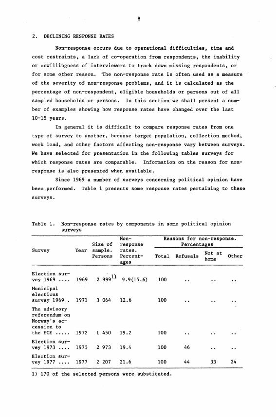
Since 1969 a number of surveys concerning political opinion have
been performed. Table 1 presents some response rates pertaining to these
surveys.
Table 1. Non-response rates by components in some political opinionsurveys
Survey
Non- Reasons for non-response.Size of response Percentages
Year sample. rates.Not at
Persons Percent- Total Refusals Otherhome
ages
Election sur- •vey 1969 1969 2 999
1)9.9(15.6) 100 • • • • . .
Municipalelectionssurvey 1969 1971 3 064 12.6 100 • • • •
The advisoryreferendum onNorway's ac-cession tothe ECE 1972 1 450 19.2 100 .. .. ..
Election sur-vey 1973 1973 2 973 19.4 100 46 •• ••
Election sur-vey 1977 1977 2 207 21.6 100 44 33 24
1) 170 of the selected persons were substituted.
Size ofYear sample.
Households
Non-responserates.Percentages
Reasons for non-response.Percentages
Not athome
Total Refusals Other
9
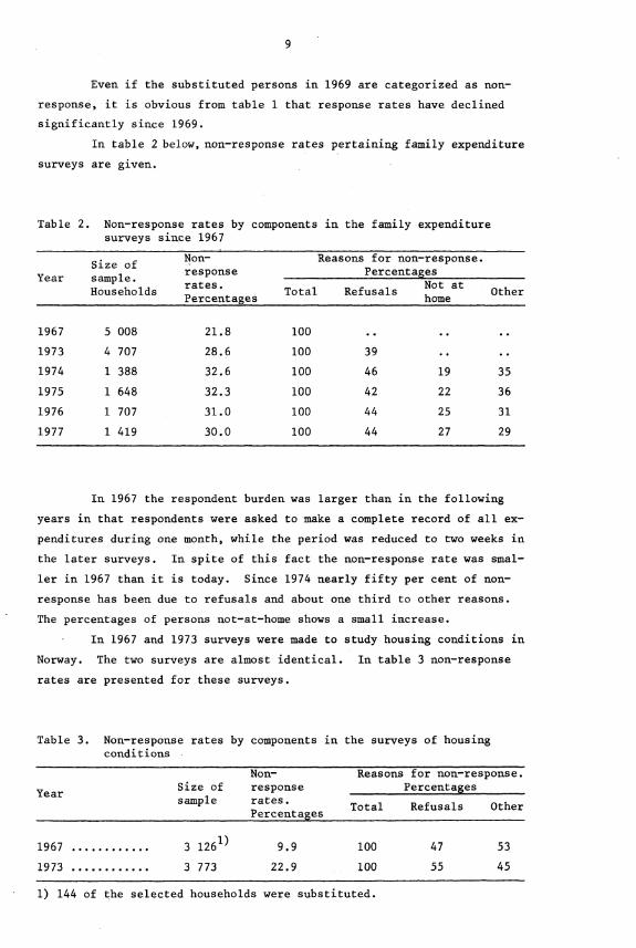
Even if the substituted persons in 1969 are categorized as non-
response, it is obvious from table 1 that response rates have declined
significantly since 1969.
In table 2 below, non-response rates pertaining family expenditure
surveys are given.
Table 2. Non-response rates by components in the family expendituresurveys since 1967
1967 5 008 21.8 100 .. .. ..
1973 4 707 28.6 100 39 .. ..
1974 1 388 32.6 100 46 19 35
1975 1 648 32.3 100 42 22 36
1976 1 707 31.0 100 44 25 31
1977 1 419 30.0 100 44 27 29
In 1967 the respondent burden was larger than in the following
years in that respondents were asked to make a complete record of all ex-
penditures during one month, while the period was reduced to two weeks in
the later surveys. In spite of this fact the non-response rate was smal-
ler in 1967 than it is today. Since 1974 nearly fifty per cent of non-
response has been due to refusals and about one third to other reasons.
The percentages of persons not-at-hom shows a small increase.
In 1967 and 1973 surveys were made to study housing conditions in
Norway. The two surveys are almost identical. In table 3 non-response
rates are presented for these surveys.
Table 3. Non-response rates by components in the surveys of housingconditions
Year
Non-Size of responsesample rates.
Percentages
Reasons for non-response.Percentages
Total Refusals Other
1967 3 1261) 9.9 100 47 53
1973 3 773 22.9 100 55 45
1) 144 of the selected households were substituted.

Non-response
Size rates inof firstsample stage.
Percent-ages
Finalnon-responserates.Percent-ages
Reasons for non-response.Percentages
Notat Othershome
TotalRefu-sals
10
As tables 1 and 2, table 3 shows an increase in non-response
rates even when the substituted households are included as non-response.
Also table 3 seems to indicate a larger proportion of refusals in 1973
than in 1967. This, however, is not observed in other surveys.
Since 1972 labour force surveys have been performed quarterly.
Table 4 presents some non-response rates pertaining to these surveys.
Two rates are given; non-response in first stages, which is the amount
of non-response after terminating the ordinary data collection. In the
second stage extra call-backs are done by telephone and by specially
trained interviewers to reduce non-response. The rates of non-response
after this collection are called final non-response rates in table 4.
Table 4. Non-response rates by components in the labour force surveys
2. quarter 1972 11 206 8.4 7.3 100 53 39 8
3. II 1972 11 180 9.5 8.2 100 45 31 24
4. .0 1972 11 039 8.8 7.8 100 .. .. ..
1. quarter 1973 10 715 8.3 7.2 100 .. .. ..
2. II 1973 10 886 10.5 9.5 100 .. .. ..
3. It 1973 11 184 10.6 9.7 100 .. .. ..
4. n 1973 11 115 10.9 8.6 100 .. .. 4..
1. quarter 1974 10 846 9.5 7.2 100 48 42 10
2. vt 1974 11 183 10.6 8.8 100 41 42 17
3. It 1974 11 512 8.0 5.6 100 44 45 11
4. It 1974 11 422 9.2 7.3 100 41 36 23
1. quarter 1975 14 153 12.6 8.3 100 48 35 17
2. It 1975 11 921 11.1 7.4 100 45 43 12
3. It 1975 11 727 12.1 8.5 100 46 42 12
4. II 1975 11 866 12.2 7.5 100 42 35 23
1. quarter 1976 11 704 15.0 10.4 100 50 30 20
2. " 1976 11 532 14.5 9.9 100 45 38 17
3. II 1976 11 418 12.8 9.1 100 47 38 15
4. It 1976 11 309 16.5 9.8 100 45 37 18
(cont.)
Non-response
. Size rates inof firstsample stage.
Percent-ages
Finalnon-responserates.Percent-ages
Reasons for non-response.Percentages
Notat Othershome
TotalRefu-sals
11
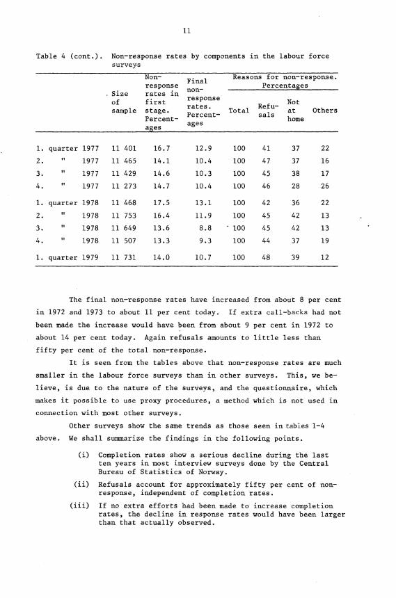
Table 4 (cont.). Non-response rates by components in the labour forcesurveys
1. quarter 1977 11 401 16.7 12.9 100 41 37 22
2. ,, 1977 11 465 14.1 10.4 100 47 37 16
3. ty 1977 11 429 14.6 10.3 100 45 38 17
4. II 1977 11 273 14.7 10.4 100 46 28 26
1. quarter 1978 11 468 17.5 13.1 100 42 36 22
2. II 1978 11 753 16.4 11.9 100 45 42 13
3. It 1978 11 649 13.6 8.8 ' 100 45 42 13
4. i, 1978 11 507 13.3 9.3 100 44 37 19
1. quarter 1979 11 731 14.0 10.7 100 48 39 12
The final non-response rates have increased from about 8 per cent
in 1972 and 1973 to about 11 per cent today. If extra call-backs had not
been made the increase would have been from about 9 per cent in 1972 to
about 14 per cent today. Again refusals amounts to little less than
fifty per cent of the total non-response.
It is seen from the tables above that non-response rates are much
smaller in the labour force surveys than in other surveys. This, we be-
lieve, is due to the nature of the surveys, and the questionnaire, which
makes it possible to use proxy procedures, a method which is not used in
connection with most other surveys.
Other surveys show the same trends as those seen in tables 1-4
above. We shall summarize the findings in the following points.
(i) Completion rates show a serious decline during the lastten years in most interview surveys done by the CentralBureau of Statistics of Norway.
(ii) Refusals account for approximately fifty per cent of non-response, independent of completion rates.
(iii) If no extra efforts had been made to increase completionrates, the decline in response rates would have been largerthan that actually observed.

12
A number of experiments have been conducted to reduce or reverse
the trend towards declining response rate. Such experiments include ex-
tensive use of telephone, call-backs by specially trained interviewers,
writing letters to refusals to explain the goals of the survey and how
important it is that they co-operate, etc. Some of these experiments have
produced an increase in the response rate, but they have given very little
insight into the reasons why completion rates decline.
Such intensive follow-up of non-respondents leads to a consider-
able increase in costs, and at present we are uncertain as to whether this
increase in costs can be justified in terms of the amount of additional
information collected. One way to study this problem is suggested in
chapter 6.
3. FACTORS EFFECTING NON-RESPONSE
3.1. Strategies for the analysis of non-response data
To give a complete analysis of which factors affect non-response,
and measure their relative contribution to the non-response rates, is a
very complex task. For example, non-response rates depend on factors
like
a. Contents of survey
b. Data collection methods
c. Attitudes among respondents
The two first factors may be partly controlled by the statistical organiz-
ation, while the last factor is only indirectly influenced by decisions
made by persons responsible for the survey operations.
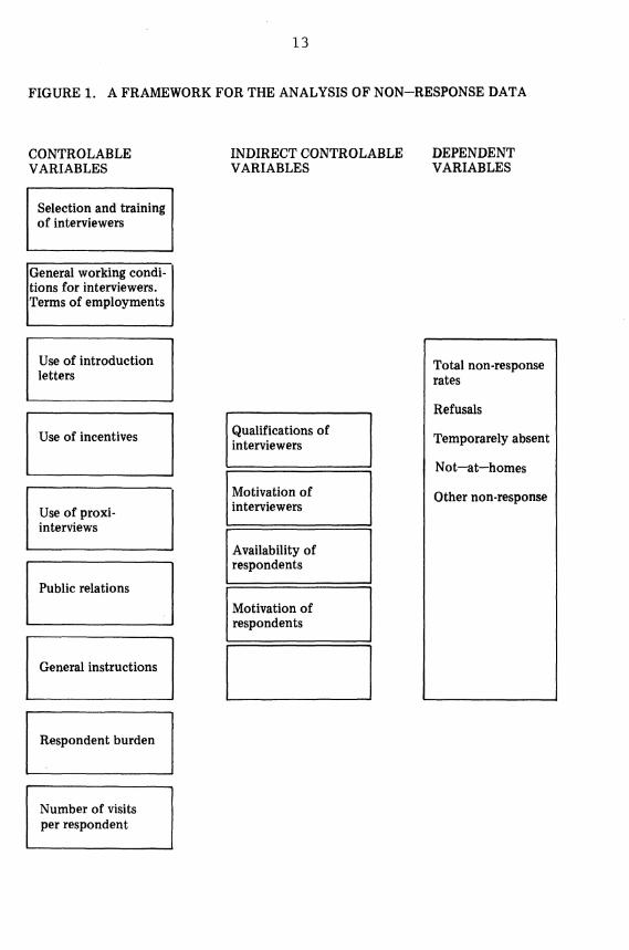
Nevertheless, in order to bring some structure into the analysis,
it is convenient to divide the variables involved into three groups:
a) The dependent variable, non-response.
b) Indirect controlable variables, which are supposed to havean effect on non-response rates, but are only indirect in-fluenced by decisions made by the survey maker.
c) Controlable variables over which the survey maker has more(or less) direct control, for example, selection and trainingof interviewers, collection methods, etc.
The distinction between category b) and c) can often cause pro-
blems, but we believe that the classification used in figure 1 is useful
in many interview surveys.
13
FIGURE 1. A FRAMEWORK FOR THE ANALYSIS OF NON—RESPONSE DATA
INDIRECT CONTROLABLE DEPENDENTVARIABLES VARIABLES
CONTROLABLEVARIABLES
Selection and trainingof interviewers
General working condi-tions for interviewers.Terms of employments
Use of introductionletters
Use of incentives
Use of proxi-interviews
Public relations
General instructions
Respondent burden
Number of visitsper respondent
Qualifications ofinterviewers
Motivation ofinterviewers
Availability ofrespondents
Motivation ofrespondents
Total non-responserates
Refusals
Temporarely absent
Not—at—homes
Other non-response

14
In most practical cases it is difficult to measure how the control-
able variables affect the indirect controlable variables, primarily be-
cause it is difficult to measure most of the indirect controlable vari-
ables. We believe, however, that there are important conceptual dif-
ferences between the two kinds of variables, which makes it useful to
distinguish between them.
Below we shall give a description of what is done in Norway to
estimate the effects of the controlable variables upon the dependent
variables. In most cases we have estimated the marginal or partial effects
of each of the controlable variables on response rates, while studies con-
cerning the simultaneous effects of the controlable variables are lacking,
due to the practical difficulties involved in doing such studies.
3.2. Selection and training of interviewers
When an interviewer is needed in an area, advertisements are pub-
lished in the local papers. Every person responding to this advertisement
receives a letter in return, in which is enclosed some information about
the Central Bureau of Statistics in general, and more specific information
concerning the Interview Survey Division. To test whether this infor-
mation is understood correctly, the person is asked to work out some pro-
blems, and the answers are returned to the central staff. Based on the
outcome of this test, a second instruction letter with problems to be
solved is issued. This procedure is repeated three times before the
central staff makes its final choice of interviewer. Shortly after a
person is hired as interviewer, he or she is requested to participate in
a three days introductory course. The total costs of appointing an inter-
viewer and give him or her the basic training amounts to some N.kr 4 500,-
(about US $ 900-).
In general, any interviewer can be assigned to any kind of survey.
In connection with the Norwegian Fertility Survey, however, it was decided
to make a selection of interviewers. Only female interviewers were assig-
ned to this survey.
3.2.1. Interviewer profile
It seems natural to expect that the interviewers' personal
characteristics have an influence on the quality of the results obtained.
We know that the sex of the interviewer has a significant influence on
the answers to some questions, but when it comes to non-response rates,
sex does not seem to have any effect.
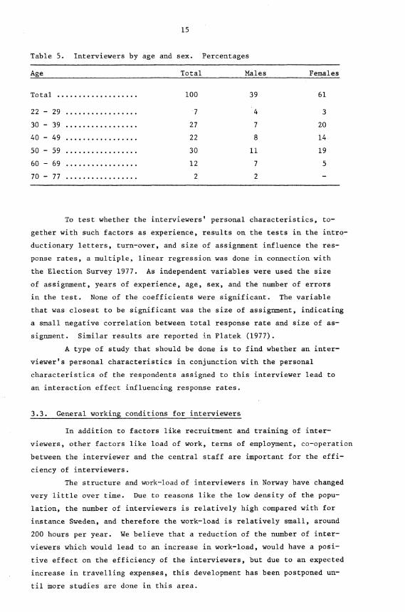
In table 5 is given the age and sex distribution of the inter-
viewers.
15
Table 5. Interviewers by age and sex. Percentages
Age Total Males Females
Total 100 39 61
22 - 29 7 4 3
30 - 39 27 7 20
40 - 49 22 8 14
50 - 59 30 11 19
60 - 69 12 7 5
70 - 77 2 2
To test whether the interviewers' personal characteristics, to-
gether with such factors as experience, results on the tests in the intro-
ductionary letters, turn-over, and size of assignment influence the res-
ponse rates, a multiple, linear regression was done in connection with
the Election Survey 1977. As independent variables were used the size
of assignment, years of experience, age, sex, and the number of errors
in the test. None of the coefficients were significant. The variable
that was closest to be significant was the size of assignment, indicating
a small negative correlation between total response rate and size of as-
signment. Similar results are reported in Platek (1977).
A type of study that should be done is to find whether an inter-
viewer's personal characteristics in conjunction with the personal
characteristics of the respondents assigned to this interviewer lead to
an interaction effect influencing response rates.
3.3. General working conditions for interviewers
In addition to factors like recruitment and training of inter-
viewers, other factors like load of work, terms of employment, co-operation
between the interviewer and the central staff are important for the effi-
ciency of interviewers.
The structure and work-load of interviewers in Norway have changed
very little over time. Due to reasons like the low density of the popu-
lation, the number of interviewers is relatively high compared with for
instance Sweden, and therefore the work-load is relatively mall, around
200 hours per year. We believe that a reduction of the number of inter-
viewers which would lead to an increase in work-load, would have a posi-
tive effect on the efficiency of the interviewers, but due to an expected
increase in travelling expenses, this development has been postponed un-
til more studies are done in this area.
16
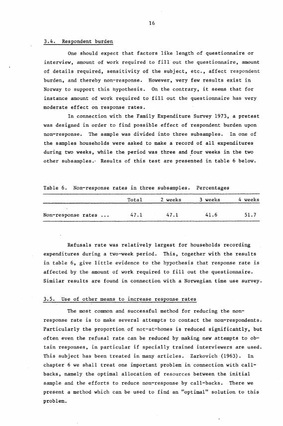
3.4. Respondent burden
One should expect that factors like length of questionnaire or
interview, amount of work required to fill out the questionnaire, amount
of details required, sensitivity of the subject, etc., affect respondent
burden, and thereby non-response. However, very few results exist in
Norway to support this hypothesis. On the contrary, it seems that for
instance amount of work required to fill out the questionnaire has very
moderate effect on response rates.
In connection with the Family Expenditure Survey 1973, a pretest
was designed in order to find possible effect of respondent burden upon
non-response. The sample was divided into three subsamples. In one of
the samples households were asked to make a record of all expenditures
during two weeks, while the period was three and four weeks in the two
other subsamples.- Results of this test are presented in table 6 below.
Table 6. Non-response rates in three subsamples. Percentages
Total 2 weeks 3 weeks 4 weeks
Non-response rates . 47.1 47.1 41.6 51.7
Refusals rate was relatively largest for households recording
expenditures during a two-week period. This, together with the results
in table 6, give little evidence to the hypothesis that response rate is
affected by the amount of work required to fill out the questionnaire.
Similar results are found in connection with a Norwegian time use survey.
3.5. Use of other means to increase response rates
The most common and successful method for reducing the non-
response rate is to make several attempts to contact the non-respondents.
Particularly the proportion of not-at-homes is reduced significafttly, but
often even the refusal rate can be reduced by making new attempts to ob-
tain responses, in particular if specially trained interviewers are used.
This subject has been treated in many articles. Zarkovich (1963). In
chapter 6 we shall treat one important problem in connection with call-
backs, namely the optimal allocation of resources between the initial
sample and the efforts to reduce non-response by call-backs. There we
present a method which can be used to find an "optimal" solution to this
problem.

17
The effect of incentives on the response rates has been studied
in some pretests, but the results from these studies have not given any
clear indications of the effectiveness of response incentives in terms
of higher response rates. However, there seems to be a positive effect
in terms of the interviewers' attitudes towards their own work.
Two of the most important factors affecting non-response are the
attitude of the general public towards the usefulness of the surveys and
the ability of the statistical office to keep selected information con-
fidential. It is therefore important to inform the general public about
how the results from the different surveys are applied by governmental
and other organizations, and what is done to improve confidentiality
safeguards and computer security within the statistical office. To give
quantitative measures of the efficiency of such activities is, however,
very difficult.
4. NON-RESPONSE EFFECTS ON SURVEY RESULTS
4.1. Introduction
In the preceding chapters we have been concerned with factors
affecting response rates. In this chapter we shall discuss an even more
complex problem, namely the effects . non-response have on theY results from
a survey. We shall first present some examples in which information about
non-respondents is collected from other sources. Cases where this is
possible are rare in practice, even in countries with good registers, like
the Scandinavian countries. Therefore, we shall suggest two methods by
which the effects of non-response can be analyzed within the sampled data.
One of the methods, which is widely used, consists of comparing the dis-
tribution of one or two variables in the sample with that or those in the
population when available. The second method, which only has received
little attention in the sampling literature, consists of making separate
analysis of data collected on the first call, the second call, etc. By
studying the differences between the results from such analysis, one can
often gain considerable insight into the effects of non-response. In
chapter 6 we formalize this approach into a probabilistic model for non-
response.
4.2. Use of alternative data sources for determining effects of non-response
In Norway a number of registers are available, which makes it
possible in some cases to obtain information on variables concerning non-
responses. This possibility has only been used in a few cases due to
18
costly data processing. In the future with more efficient data processing
systems, we expect to conduct a number of studies using register-data to
determine the effects of non-response. In this section we shall give some
examples of such studies.
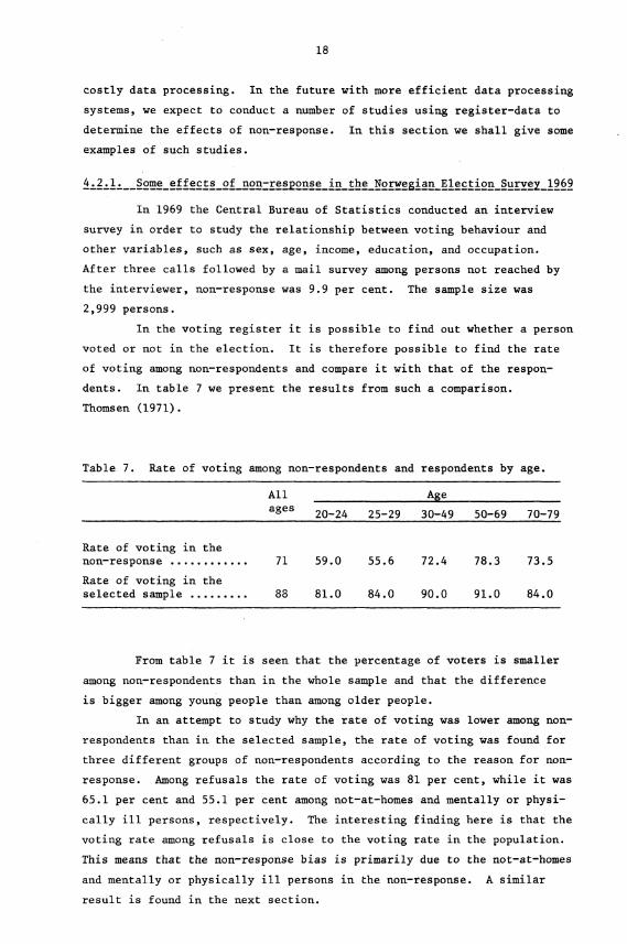
4.2.1. Some effects of non-response in the Norwegian Election Survey 1969
In 1969 the Central Bureau of Statistics conducted an interview
survey in order to study the relationship between voting behaviour and
other variables, such as sex, age, income, education, and occupation.
After three calls followed by a mail survey among persons not reached by
the interviewer, non-response was 9.9 per cent. The sample size was
2,999 persons.
In the voting register it is possible to find out whether a person
voted or not in the election. It is therefore possible to find the rate
of voting among non-respondents and compare it with that of the respon-
dents. In table 7 we present the results from such a comparison.
Thomsen (1971).
Table 7. Rate of voting among non-respondents and respondents by age.
All
Ageages 20-24 25-29 30-49 50-69 70-79
Rate of voting in thenon-response 71 59.0 55.6 72.4 78.3 73.5
Rate of voting in theselected sample 88 81.0 84.0 90.0 91.0 84.0
From table 7 it is seen that the percentage of voters is smaller
among non-respondents than in the whole sample and that the difference
is bigger among young people than among older people.
In an attempt to study why the rate of voting was lower among non-
respondents than in the selected sample, the rate of voting was found for
three different groups of non-respondents according to the reason for non-
response. Among refusals the rate of voting was 81 per cent, while it was
65.1 per cent and 55.1 per cent among not-at-homes and mentally or physi-
cally ill persons, respectively. The interesting finding here is that the
voting rate among refusals is close to the voting rate in the population.
This means that the non-response bias is primarily due to the not-at-homes
and mentally or physically ill persons in the non-response. A similar
result is found in the next section.
19
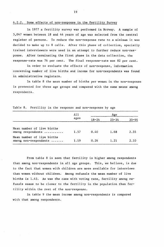
4.2.2. Some effects of non-resRonse in the Fertility Survey
In 1977 a fertility survey was performed in Norway. A sample of
5,047 women between 18 and 44 years of age was selected from the central
register of persons. To reduce the non-response rate to a minimum it was
decided to make up to 8 calls. After this phase of collection, specially
trained interviewers were used in an attempt to further reduce non-res-
ponse. After terminating the first phase in the data collection, the
response-rate was 76 per cent. The final response-rate was 82 per cent.
In order to evaluate the effects of non-response, information
concerning number of live births and income for non-respondents was found
in administrative registers.
In table 8 the mean number of births per woman in the non-response
is presented for three age groups and compared with the same means among
respondents.
Table 8. Fertility in the response and non-response by age
All
Ageages
18-24 25-34 35-44
Mean number of live birthsamong respondents
1.57 0.40
1.68 2.55
Mean number of liye birthsamong non-respondents
1.19 0.26
1.21 2.10
From table 8 is seen that fertility is higher among respondents
than among non-respondents in all age groups. This, we believe, is due
to the fact that women with children are more available for interviews
than women without children. Among refusals the mean number of live
births is 1.43. As was the case with voting rate fertility among re-
fusals seems to be closer to the fertility in the population than fer-
tility within the rest of the non-response.
In table 9 the mean income among non-respondents is compared
with that among respondents.

20
Table 9. Mean income in the response and non-response by age.N.kr. 100.00
Allages
Age
18-24 25-34 35-44
Mean income among respondents
Mean income among non-respondents
677.3
581.7
340.4
272.4
757.8
612.0
888.8
862.2
It is seen in table 9 that income among non-respondents is lower
than income among respondents, a finding for which we do not have any
good explanation. If we again divide non-response into two groups,
"refusals" and "others", we find that mean income among refusals is
100 N.kr. 716.1, while the same figure for others is 100 N.kr. 406.5.
As was the case concerning fertility, refusals are more like the popu-
lation in income than other non-respondents.
We have presented three examples in which refusals seem to be
more like the population than the rest of the non-respondents. Further
research is planned to test this important and for many variables reason-
able hypothesis, as it is of great practical interest. See also chapter 6.
4.3. .Indirect measurement of the effects of non-response
It is seldom that information concerning non-respondents can be
found in existing registers, and therefore other techniques are usually
used to gain insight into the effects of non-response upon the results
from a survey. The simplest and most commonly used method, is to look
at the age and sex distributions in the sample and compare these with
distributions for the non-respondents. In addition, one can estimate
the correlation between the study variable and sex and/or age in the
sample, and thereby estimate the effect of non-response by assuming that
the correlation among non-respondents is the same as that found in the
sample.
In the rest of this chapter, we shall describe another method
which, in our opinion, can provide insight into the effects of non-res-
ponse and also lead to good weighting procedures to reduce the effects
of non-response. The method consists in conducting separate analysis on
data collected in the first call, the second call, the third call, etc.
The method has the advantage that it can give insight not only into the
effect of non-response when the aim is to estimate a mean in the popu-
lation, but also when the aim is to estimate relationships between two

35-44 yearsof age
25-34 yearsof age
18-24 yearsof age
•
:+:44
»:44•4.
»:44
•••4
3,0
21
FIGURE 2. MEAN NUMBER OF LIVE BIRTHS BY AGE GROUPS ANDNUMBER OF CALLS
0;•;•;4..!***
Fl Data collected inL-1.-j the first call
• Data collected inthe second call
Data collected inthe third call
Data collected afterfour or more calls
Mean number of live births
t
0.,
22
L
. :; : : :; : : :••• : :; : : - . - .. : .. . . . . . . . ....... ... .
• . • . . . • .
•• • • • • • • • • • . . . . . . . . .
:
;c1s/".
. • . . • : • : : : • : • . • •
• : • : • : • . • . • . •
• . . • ... . '
•
23
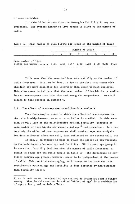
or more variables.
In table 10 below data from the Norwegian Fertility Survey are
presented. The average number of live births is given by the number of
calls.
Table 10. Mean number of live births per woman by the number of calls
Number of calls
1 2 3 4 5 6 7 8
Mean number of livebirths per woman 1.84 1.56 1.47 1.30 1.28 1.08 0.85 0.75
It is seen that the mean declines substantially as the number of
calls increases. This, we believe, is due to the fact that women with
children are more available for interview than women without children.
This also seems to indicate that the mean number of live births is smaller
in the non-response than that observed among the respondents. We shall
return to this problem in chapter 6.
4.4. The effect of non-response on multivariate analysis
Very few examples exist in which the effect of non-response on
the relationship between two or more variables is studied. In this sec-
tion we will look at the relationships between fertility (measured by
mean number of live births per woman), and age l) and education. In order
to study the effect of non-response we shall conduct separate analysis
for data collected after one call, data collected on the second call, etc.
In fig. 2, an attempt is made to study the effect of non-response
on the relationship between age and fertility. Within each age group it
is seen that fertility declines when the number of calls increases, a
result we found for the whole sample in table 10. The difference in fer-
tility between age groups, however, seems to be independent of the number
of calls. This, we find encouraging, as it seems to indicate that the
relationship between age and fertility is less affected by non-response
than fertility itself.
1) As is well known the effect of age can not be estimated from a singlesurvey. What in this section is called "effect of age" is a combinationof age, cohort, and periode effect.
24
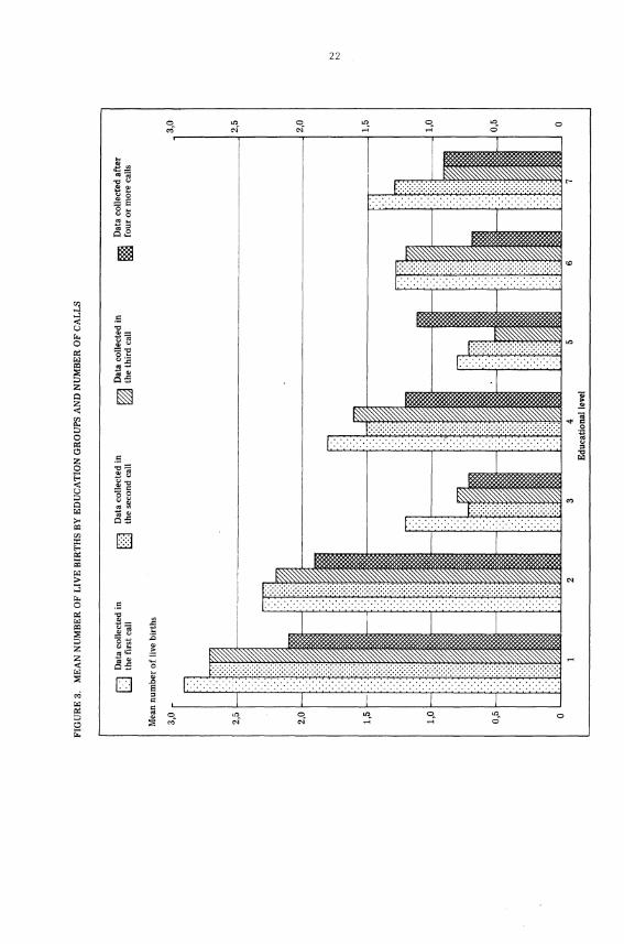
In fig. 3 a similar study is made * concerning the relationship
between education and fertility. The respondents are classified into
one of seven groups by their highest completed education. These groups
are:
Group 1: Primary school, lower stage
Group 2: Continuation school
Group 3: Education at second level, first stage
Group 4: Education at second level, second stage I
Group 5: Secondary general school, upper stage
Group 6: Education at second level, second stage II
Group 7: Education at third level
Fig. 3 seems to indicate that also the relationship between edu-
cation and fertility is less affected by non-response than fertility it-
self.
To pursue this point a little further, we shall study the simul-
taneous relationship between fertility, age and education, and see how
this analysis is affected by non-response. The technique we shall use
is standardization as suggested in Pullman (1978).
Before doing the analysis we shall give a short description of
the model and the estimation methods applied.
Suppose that we are interested in the relationship between
fertility, y (measured as the number of live births) and explanatory
variables education, x l , and age, x2 . We also assume that, measured
in a suitable way, the relationship is linear.
(4.1) y = b ixi + b 2x2 + co + residual
Between age and education we also assume a linear relationship
(4.2) xl = b 12x2 cl residual.
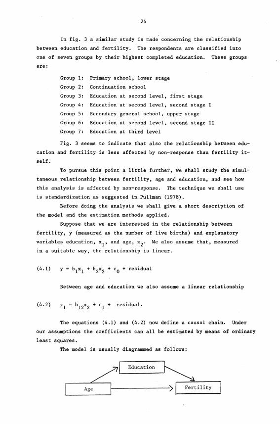
The equations (4.1) and (4.2) now define a causal chain. Under
our assumptions the coefficients can all be estimated by means of ordinary
least squares.
The model is usually diagrammed as follows:
-7
Age
25
In the Fertility Survey both explanatory variables are measured
as ordinal variables, and are therefore transformed into dummy variables.
In principle, this does not change the analysis, but the ordinary least
squares estimation method is identical with a technique known as standardi-
zation. An important advantage with this technique is that calculations
can be done directly on the basis of tables like the next one. Such tables
(based on the whole sample) are likely to be published in the report from
the survey.
In order to get an idea of what effect non-responses have on such
an analysis we shall estimate the direct and indirect effects of age on
fertility for data collected in the first call. The same analysis is
repeated for data collected in the second call, the third call, the fourth
and later calls, respectively.
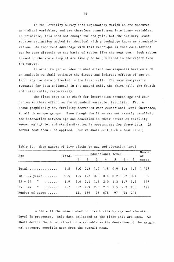
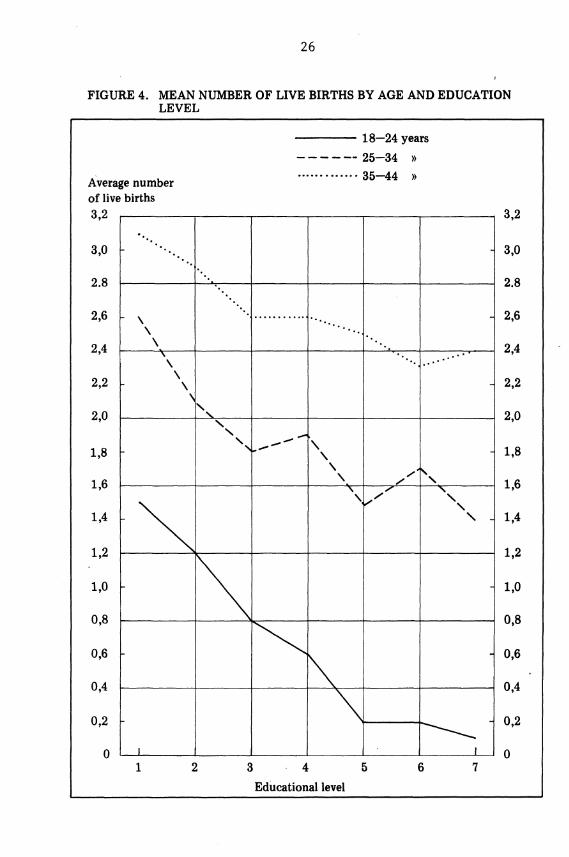
The first step is to check for interaction between age and edu-
cation in their effect on the dependent variable, fertility. Fig. 4
shows graphically how fertility decreases when educational level increases,
in all three age groups. Even though the lines are not exactly parallel,
the interaction between age and education in their effect on fertility
seems negligible, and standardization is appropriate for these data. (A
formal test should be applied, but we shall omit such a test here.)
Table 11. Mean number of live births by age and education level
Age TotalEducational level
Numberofcases1 2 3 4 5 6 7
Total 1.8 3.0 2.3 1.2 1.8 0.9 1.4 1.7 1 478
18 - 24 years 0.5 1.5 1.2 0.8 0.6 0.2 0.2 0.1 339
25 - 34 1.9 2.6 2.1 1.8 2.0 1.3 1.7 1.5 667
35 - 44 11 2.7 3.2 2.9 2.6 2.5 2.5 2.3 2.5 472
Number of cases 121 189 98 678 97 94 201
In table 11 the mean number of live births by age and education
level is presented. Only data collected at the first call are used. We
shall define the total effect of a variable as the deviation of the margi-
nal category specific mean from the overall mean.
1 2 3 4 5 6 7
18-24 years
— — 25-34 » 35-44 »
. .. . ... . . .. .
_\••
•
,............
... , •• ..... .. ....,
. . ......
_•••
••■
.•••••••••••••
_
••\•-■.--'"-\
•••
■-// \
_
•• .//
•••\
_
_
_
i i
Educational level
Average numberof live births3,2
3,0
2.8
2,6
2,4
2,2
2,0
1,8
1.6
1.4
1.2
1.0
0.8
0.6
0.4
0,2
0
3,2
3,0
2.8
2,6
2,4
2,2
2,0
1,8
1,6
1,4
1,0
0,8
0,6
0,4
0,2
0
26
FIGURE 4. MEAN NUMBER OF LIVE BIRTHS BY AGE AND EDUCATIONLEVEL
27
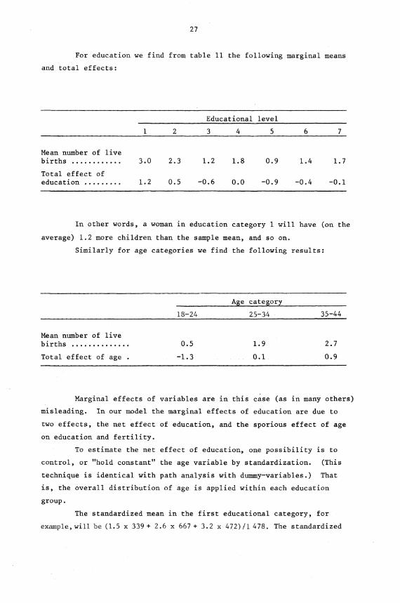
For education we find from table 11 the following marginal means
and total effects:
Educational level
1 2 3 4 5 6
3.0
1.2
2.3
0.5
1.2
-0.6
1.8
0.0
0.9
-0.9
1.4
-0.4
1.7
-0.1
Mean number of livebirths
Total effect ofeducation
In other words, a woman in education category 1 will have (on the
average) 1.2 more children than the sample mean, and so on.
Similarly for age categories we find the following results:
Age category
18-24
25-34
35-44
Mean number of livebirths 0.5 1.9 2.7
Total effect of age . -1.3 0.1 0.9
Marginal effects of variables are in this case (as in many others)
misleading. In our model the marginal effects of education are due to
two effects, the net effect of education, and the sporious effect of age
on education and fertility.
To estimate the net effect of education, one possibility is to
control, or "hold constant" the age variable by standardization. (This
technique is identical with path analysis with dummy-variables.) That
is, the overall distribution of age is applied within each education
group.
The standardized mean in the first educational category, for
example, will be (1.5 x 339+ 2.6 x 667+ 3.2 x 472)/1 478. The standardized
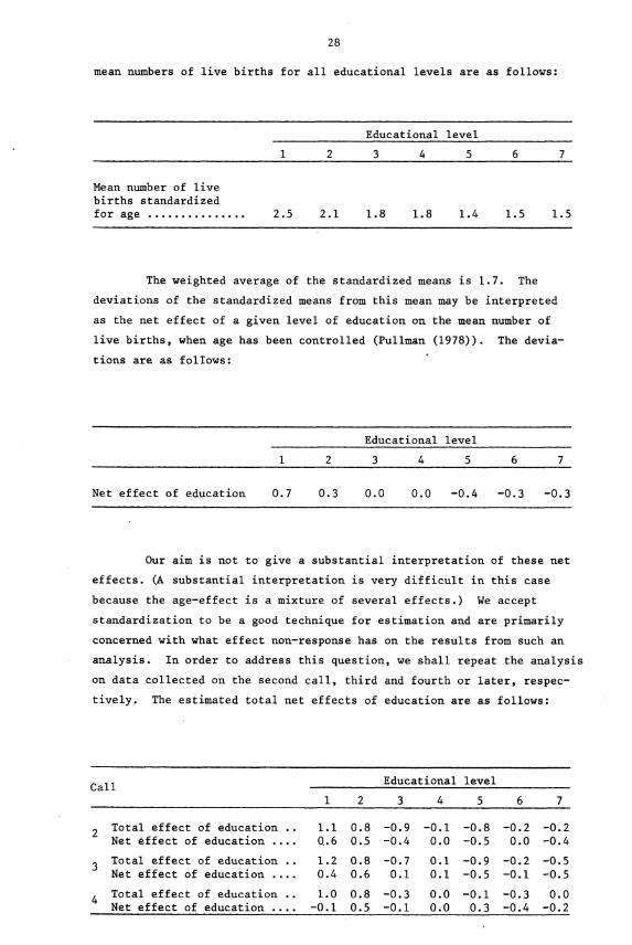
28
mean numbers of live births for all educational levels are as follows:
Educational level
1 2 3 4 5
6 7
Mean number of livebirths standardizedfor age 2.5 2.1 1.8 1.8 1.4 1.5 1.5
The weighted average of the standardized means is 1.7. The
deviations of the standardized means from this mean may be interpreted
as the net effect of a given level of education on the mean number of
live births, when age has been controlled (Pullman (1978)). The devia-
tions are as follows:
Educational level
1 2 3 4 5 6
Net effect of education 0.7 0.3 0.0 0.0 -0.4 -0.3 -0.3
Our aim is not to give a substantial interpretation of these net
effects. (P, substantial interpretation is very difficult in this case
because the age-effect is a mixture of several effects.) We accept
standardization to be a good technique for estimation and are primarily
concerned with what effect non-response has on the results from such an
analysis. In order to address this question, we shall repeat the analysis
on data collected on the second call, third and fourth or later, respec-
tively. The estimated total net effects of education are as follows:
CallEducational level
1 2 3 4 5
6 7
2 Total effect of education ..Net 6ffect of education ....
Total effect of education ..3
Net effect of education ....
Total effect of education ..4Net effect of education ....
1.1 0.8 -0.9 -0.1 -0.8 -0.2 -0.2
Q.6 0.5 -0.4 0.0 -0.5 0.0 -0.4
1.2 0.8 -0.7 0.1 -0.9 -0.2 -0.50.4 0.6 0.1 0.1 -0.5 -0.1 -0.5
1.0 0.8 -0.3 0.0 -0.1 -0.3 0.0
-0.1 0.5 -0.1 0.0 0.3 -0.4 -0.2
29
The mean number of live births varies from 1.8 to about 1.0 in
the four sets of data. This, we believe, is due to the fact that women
with children are more available for interview than women with few or no
children. The analysis done in this section aims at answering the ques-
tion whether non-response has any effect on the relationship between age,
education, and fertility. The results seem to indicate that there is
very little or no systematic effect of non-response on the relationships
between the three variables.
5. METHODS TO REDUCE THE EFFECTS OF NON-RESPONSE
5.1. Introduction
In chapter 4 it was shown that non-response can lead to seriously
biased results, and many other examples of this can be found in the lite-
rature, Zarkovich (1966).
It is generally accepted that the best way of reducing bias due
to non-response is to keep response rates at maximal level through effec-
tive operational procedures. However, after the data collection is ter-
minated, there will always remain some non-response, and it is natural to
raise the question whether the bias due to non-response can be reduced by
applying special estimation techniques. Many techniques have been sugges-
ted, the most well-known are:
(i) Post-stratification
(ii) The Politz-Simmon method
(iii) Bartholomew's method
In Norway we have never used the Politz-Simmon method, while the
other two methods have been used on several occasions. In this chapter
we shall give a few examples illustrating the use of these two methods.
In chapter 6 we shall suggest a new weighting procedure, and apply this
method to data from the Norwegian Fertility Survey.
5.2. Post-stratification
The technique of post-stratification was used in the household
expenditure surveys. The response problem is particularly important for
these surveys, because response rates in general are smaller than normally
encountered. Also, it is known that response rates vary between sub-
classes, which are homogeneous with respect to expenditure. To evaluate
the efficiency of post-stratification, the following expression for the
bias due to non-response is useful, Thomsen (1973),

30
L L(5.1) Bias = (1/E) E i''W. (h.-E) + E W. (1-h.)(i!- --IP!)
'i=1 1=1
where h. is the response rate in the ith
post-stratum, h = E W,h.,1
i=1
W. is the proportion of the population in the i th post-stratum, Y, 7.are, respectively, the respondent and non-respondent means in the
ith post-stratum.
The first term in (5.1) is the component due to different res-
ponse rates. It is the component that is reduced by post-stratification,
and it can be estimated from the sample. It should be emphasized that
(5.1) gives the bias for a given set of post-strata, and that one can
shift part of the bias between the components by choice of post-strata.
In practice it is important to choose the right variables for post-stra-
tification. Also, it is important not to make too many post-strata, be-
cause the gains from using this technique decline rapidly with an increase
in the number of post-strata. In addition, having too many post-strata
would result in some post-strata having no respondents.
In the Household Expenditure Survey, a good variable for post-
stratification was found to be "size of household". The first component
in (5.1) is estimated for different choises of the number of post-strata.
The results are given in table 12.
Table 12. Estimates of the component due to different response ratesby the number of post-strata
Number of post-strata
2
3 4
5
Estimates of the componentdue to different responserates
Nkr 215 Nkr 296 Nkr 326 Nkr 335
It is seen that the gains from using post-stratification decline
rapidly with the number of post-strata.
The second component in (5.1) is usually not known, as Ý. is un-
known. One therefore has to make some assumptions concerning the second
component to be able to evaluate the effect of post-stratification on the
total bias. The first component gives the maximum reduction of the bias
when post-stratification is used.
31
We shall now give an example in which the second component can
be estimated because information concerning non-respondents is available
from registers. Data are taken from the Fertility Survey, the study
variable is "number of live births", while the post-stratification vari-
ables are "age" and "marital status". The sample was divided into six
post-strata, three age groups, and two marital status groups. Among
respondents the average number of live births per woman is 1.57, while
the same average is 1.50 in the selected sample. The total bias due to
non-response is 0.07.
To evaluate the efficiency of post-stratification the first term
of (5.1) was estimated to be 0.05, from which follows that the estimate
of the remaining bias after post-stratification is 0.02.
In this case the use of post-stratification has eliminated slightly
more than 70 per cent of the non-response bias. This may not be surprising
as the correlation between the post-stratification variables and the study
variable is very high.
5.3. Bartholomew's method
In Bartholomew (1961) is suggested a method for reducing non-
response bias, the method consists of giving different weights to results
from the first and second call. The estimator is as follows:
11 -- n
, n11,-Y = - Y + -n )Y21'B n 11
where Yil and i'21 are the sample means in the first and second call res-
pectively, and n11 is the number of elements interviewed in the first
call.
The method is useful when one has information indicating that the
mean in the second call is closer to the mean in the non-response than
the mean in the first call.
6. A PROBABILISTIC MODEL FOR NON-RESPONSE
6.1. Introduction
In this chapter we shall present a probabilistic model for non-
response. This model gives rise to an estimable variance, and estimable
non-response bias, and an estimable cost. The model is applied in con-
nection with the Fertility Survey to find a new adjusting method for non-
response bias. Also, the model is used to study the relationship between

32
the mean square error and the number of call-backs, and the results are
used to evaluate the allocation of resources between the initial sample
and the efforts to reduce non-response by call-backs. Finally, we study
the effects of non-response on measures of association between fertility
and other variables.
It should be noticed that the fitting of the model to data from
the Fertility Survey is tentative, and that modifications are suggested
several places. This application of the model is included primarily to
demonstrate the potentials of the model. Later we intend to publish the
final results in an independent publication.
6.2. The model
When an interviewer makes an attempt to interview a selected
household, there are three possible outcomes:
(i) The interviewer gets a response.
(ii) The interviewer gets no response and decides to call back.
(iii) The interviewer gets no response and decides to categorizethe household as non-response (refusal).
In practice it is well known that it is difficult for the interviewer to
distinguish between permanent and temporary refusals, but in this con-
nection the important thing is that such a categorization is done after
each visit.
Let p denote the probability that outcome (i) occurs in the first
call, and let f denote the probability that outcome (iii) occurs in the
first visit. We now assume that f is constant in the successive visits,
but that outcome (i) occurs with probability Ap in the second and fol-
lowing calls. We also expect A to be larger than one because the inter-
viewers use ingenuity. They find out from neighbours or parents when
the people now absent will be available. They make appointments etc.
The result of this is, expectedly, that the probability of getting a
response should increase after the first call.
In Figure 5 below the model is shown in a diagram.
Let C denote the outcome that the interviewer gets a response
from a selected household in the C th visit, then
P(C=1) = p
P(C=2) = (1 - p - f)Ap
P(C=3) = (1 - p - f)(1 - Ap - f)Ap
P(C=c) = {I)(1 - p - f)(1 - Ap - f)
c-2Ap
if c = 1if c 2

(1-13-0
Non.response
Non-response
P Response
••••
Lean 2. call
Response
3. call
Response
Non-response
Callback
33
FIGURE 5. A PROBABILISTIC MODEL FOR NON— RESPONSE
The parameters p, A, and f can be estimated from the sample, assuming
that information concerning the number of calls for each selected house-
hold is available.
The model can be generalized by allowing p to vary between the
households or persons. One possibility is to assume that p is generated
by a Beta-distribution, while another is to assume that p is constant
within certain subclasses in the population, but varies between them.
In what follows we shall assume that the parameters are constant
within certain subclasses, called post-strata, but vary between them.
This model is similar to a number of other non-response models, but also
differs from them in important aspects.
The rational behind the correction method introduced in
Bartholomew (1961) is that the interviewer in the second call is able to
get responses from a sample representative for the non-respondents in
the first call. In our model this means that the conditional probability
of being a respondent in the second call, given that it was a non- res-
pondent in the first call, is the same for all post-strata.
Our model is also similar to the probabilistic model suggested
in Deming (1953). The most important difference is that the possibility
to estimate the parameters in the model is ignored in Deming (1953).
The model presented In this paper is similar to the model suggested

34
in Politz and Simmon (1949) in that it considers availability to be im-
portant when correcting for non-response bias. In Politz and Simmon
(1949) the probability of finding a person at home is estimated by in-
cluding questions in the questionnaire to ascertain whether a respondent
was at home last night at this time, the night before last, etc., to
cover the 5 nights preceding the interview. Each response is then given
a weight wi , the reciprocal of the number of nights at home over the
period of 6 successive nights. In our model the probability of finding
a person at home is estimated by means of information concerning the
number of calls made before he/she was found at home.
A somewhat different kind of non-response model is suggested in
the literature, where it is assumed that there is a linear relationship
between the sample mean and the number of calls. Such relationships are
often observed in practice (see table 10). In our model the linear re-
lationship is due to the fact that people have different availability,
and that availability is highly correlated with a number of variables.
We shall demonstrate below two methods of estimating the para-
meters in our model. First we shall use two age groups as post-strata.
In this case the number of persons in each post-stratum is known, and
maximum likelihood estimates can be calculated. In addition, the good-
ness of fit can be evaluated.
Thereafter, we shall study the more important case in which the
number of persons within each post-stratum is unknown. In such cases
the parameters can be estimated by means of the least squares method.
The two methods are used on the same set of data for computational
convenience. In practice only one of the methods would be used on a
specific survey.
6.3. Fitting the model to data from the Fertility Survey
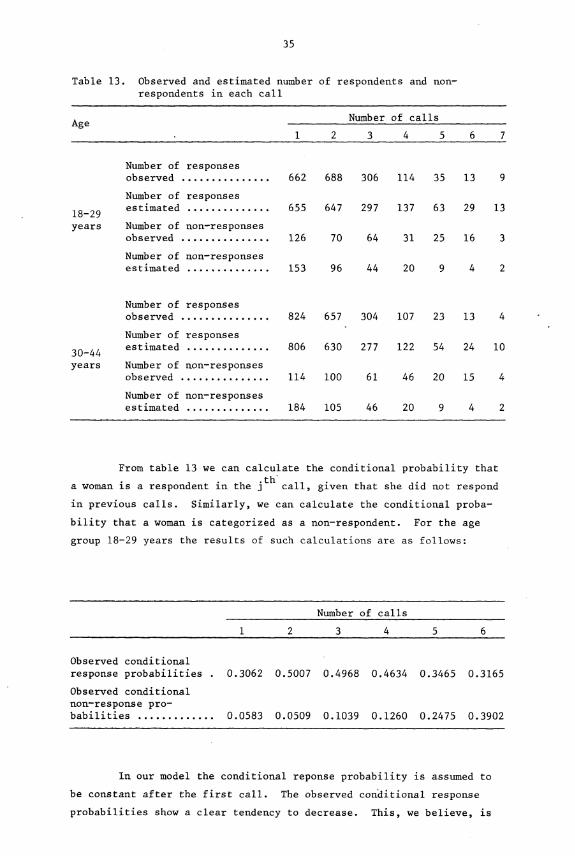
In table 13 below, the number of women categorized as responses
and non-responses in each call in the Norwegian Fertility Survey are
given within two age groups. Assuming that the parameters p, f, and
A are constant within these two age groups, pl , f l , A l , p2 , f 2 , and A2respectively, the maximum likelihood estimates are
f = 0.07 i2 = 0.08
p1 = 0.30 P2 = 0.35
1 = 1.56 R2 = 1.39
The maximum likelihood estimates are developed in Appendix 1.
35
Table 13. Observed and estimated number of respondents and non-respondents in each call
Age
Number of responsesobserved
Number of responses
18-29 estimated
years Number of non-responsesobserved
Number of non-responsesestimated
Number of responsesobserved
Number of responses
30-44 estimated
years Number of non-responsesobserved
Number of non-responsesestimated
Number of calls
1 2 3 4 5 6
662 688 306 114 35 13 9
655 647 297 137 63 29 13
126 70 64 31 25 16 3
153 96 44 20 9 4 2
824 657 304 107 23 13 4
806 630 277 122 54 24 10
114 100 61 46 20 15 4
184 105 46 20 9 4 2
From table 13 we can calculate the conditional probability that
a woman is a respondent in the j th' call, given that she did not respond
in previous calls. Similarly, we can calculate the conditional proba-
bility that a woman is categorized as a non-respondent. For the age
group 18-29 years the results of such calculations are as follows:
Number of calls
1 2 3 4 5 6
Observed conditionalresponse probabilities . 0.3062 0.5007 0.4968 0.4634 0.3465 0.3165
Observed conditionalnon-response pro-babilities 0.0583 0.0509 0.1039 0.1260 0.2475 0.3902
In our model the conditional reponse probability is assumed to
be constant after the first call. The observed conditional response
probabilities show a clear tendency to decrease. This, we believe, is

36
due to the fact that within the age-group 18-29 years the response pro-
bability is not constant, but varies between individuals. Therefore, in
the later calls the response rates will decrease, because the interviewer
will be visiting persons that are hard to find. Another reason is that
the interviewer after having done several calls has a tendency to increase
the probability of categorizing a household or person as a non-response
instead of deciding to call back.
In our model, this could be taken care of by introducing a shift
in f after the first call, and/or by allowing p to vary within the post-
strata, for instance by assuming that p is generated by a Beta-distri-
bution. We shall, however, not use such a generalization of the model
here.
In spite of the simplicity of the model, the estimates seem to
fit very well in with what one would expect. The fact that P 1 is smaller
than P 2 is known from other surveys in Norway, and in other countries as
well.
Many women in the first age-group live together with their parents
and it seems reasonable that A1 is larger than A
2 because the interviewer
through the parents has a good chance to get contact with the interviewee
in later calls. It is, in our opinion, surprising that A l and A 2 are as
large as they are. However, this seems to be the case in other surveys as
well. We shall not go further in the interpretations of the result here,
as we feel that results from more surveys must be available before such
interpretations can be of any value. In the future we intend to fit the
same model to data from other surveys and thereby, hopefully, gain more
insight into the processes generating non-response. One important ques-
tion, we think, is whether f varies so little between subclasses as in
this case. The results in chapter 4, however, do confirm that the refusal
rate varies little between subclasses in the population.
6.4. Adjusting for non-response bias
In this section we shall demonstrate how the model presented in
section 6.2 can be used when the aim is to reduce non-response bias. The
variable of interest is now "number of live births", and the aim is to
estimate the mean of this variable in the population. To do this the
population is divided into 7 groups, or post-strata. Post-stratum i con-
sists of women with i live births, i = 0,1,2,...,6. Post-stratum 6 in-
cludes women with 6 or more live births.
As in section 6.3 we assume that p and A are constant within each
post-stratum, but vary between them. In addition, we assume that f is
constant in the whole sample.

37
To estimate the mean number of live births in the population, we
must estimate the number of women in each post-stratum. Several estimation
methods are available, but in many cases the least squares method seems to
be natural.
Assume that N women have been selected in the sample, and let N.
denote the number of women selected in post-stratum i. Then the expected
number of responses in the j th call in post-stratum i is N.P(C. =
where
r pip{C i = c.} = c.-2
1 (1 - p i - f)(1 - A ip i f) 1 A ip i
if c. = 1
if c. 2
Let X. denote the observed number of responses in post-stratum i in theth
j call. The least squares estimates of A i , p i and f can now be found
by minimizing
6 8E E (N.P(C.
i=0 j=1 1 1
under the condition that
2j) - X..) ,
6E N. = N.i=0 1
In many cases the number of parameters can be reduced. In the present
case it seems reasonable to assume that
p = if3 + a + RESIDUAL,
where i is the number of live births. (See table 15.)
However, in order to make the calculations simple, we shall use
a "quick and dirty" estimation method. The method is based on data from
the three first calls, and the estimators are found as the solution to
the following equations:
Nip i = xil
N.(1-p i-f) A ip i = x i2
E
(6.1)N i (1-p i -f)(1 A. = x
i3 (1=0,1,2,...,6).
N. = 5047
38
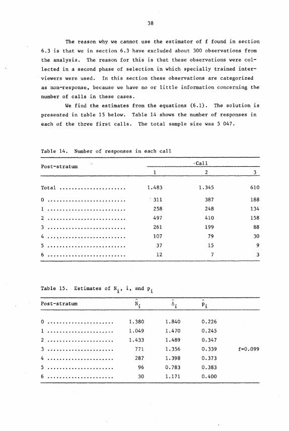
The reason why we cannot use the estimator of f found in section
6.3 is that we in section 6.3 have excluded about 300 observations from
the analysis. The reason for this is that these observations were col-
lected in a second phase of selection in which specially trained inter-
viewers were used. In this section these observations are categorized
as non-response, because we have no or little information concerning the
number of calls in these cases.
We find the estimates from the equations (6.1). The solution is
presented in table 15 below. Table 14 shows the number of responses in
each of the three first calls. The total sample size was 5 047.
Table 14. Number of responses in each call
Post-stratum•Call
1 2
Total 1.483 1.345 610
0 •311 387 188
1 258 248 134
2 497 410 158
3 261 199 88
4 107 79 30
5 37 15 9
6 12 7 3
Table 15. Estimates of Ni , i, and p i
Post-stratumAN.
AA. Pi
0 1.380 1.840 0.226
1 1.049 1.470 0.245
2 1.433 1.489 0.347
3 771 1.356 0.339 f=0.099
4 287 1.398 0.373
5 96 0.783 0.383
6 30 1.171 0.400
39
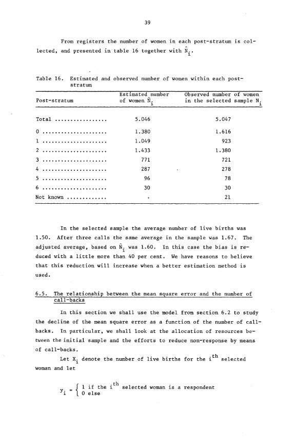
From registers the number of women in each post-stratum is col-
lected, and presented in table 16 together with Ni .
Table 16. Estimated and observed number of women within each post-stratum
Estimated number Observed number of womenPost-stratum of women Ñ. in the selected sample Ni
5.046 5.047
1.380 1.616
1.049 923
1.433 1.380
771 721
287 278
96 78
30 30
21
Total
0
1
2
3
4
5
6
Not known
In the selected sample the average number of live births was
1.50. After three calls the same average in the sample was 1.67. The
adjusted average, based on Ñ. was 1.60. In this case the bias is re-
duced with a little more than 40 per cent. We have reasons to believe
that this reduction will increase when a better estimation method is
used.
6.5. The relationship between the mean square error and the number ofcall-backs
In this section we shall use the model from section 6.2 to study
the decline of the mean square error as a function of the number of call-
backs. In particular, we shall look at the allocation of resources be-
tween the initial sample and the efforts to reduce non-response by means
of call-backs.
Let X. denote the number of live births for the i th selected
woman and let
1 if the ith selected woman is a respondentYi = 0 else

(6.2) q. -J 6 6 k
E N.p. + E E N.(1-p.-f)(1-A.p.-f) A.p.j=0 J J j=0 i=2 J J J J J J
N.p. + E N.(1-p.-f)(1-A.p.-f)1-2
A.p.J J.JJ J J J J1=2
k
1-2
40
The respondent mean can now be written as
nE Xiy i
- - i=1X s n
E y.1=1 1
where n is the sample size.
We now assume that the sample is post-stratified as in section
6.4, and let
P (A woman in the sample belongs to post-stratum j f The woman is a respondent) = q j ; j=0,1,2,...,6.
We then have that after the first call
q. - 6E N.p.
j=0 3
j =0,1,2,•••,6•N.p.33
After ka 2) calls, we have
We now have that
5(6.3) E(R ) = E jq. + 6.5 q6 ,
s j=1
and
5 n(6.4) var() [ E q.(j-E()) 2 + q
6(6.5-E(
5)) 2 1 E[ E yi ],
j=0 J 1=1
where the average number of live births per woman in post-stratum 6 is
assumed equal to 6.5.A ,
Substituting N., p., A., and f with N., p., A., and i found inJ J J A J J J
section 6.4 we find and estimate for q., q., which inserted in (6.3) and
(6.4) give us estimates of E(R s ) and var(:).

41
Furthermore,
Bias (Rs ) = E(Rs - R),
which also can be estimated as X is known is this survey.
In table 17 the estimated bias and mean square error is given as
a function of the number of calls.
Table 17. Estimated bias and mean square error by the number of calls
Number of calls
1 2 3 4 5 6 7 8 9 10
Bias 0.339 0.207 0.166 0.144 0.133 0.127 0.123 0.122 0.121 0.120
Mean squareerror 0.1162 0.0435 0.0281 0.0212 0.0182 0.0166 0.0156 0.0153 0.0151 0.0149
Mean squareerror 0.3408 0.2085 0.1676 0.1457 0.1347 0.1288 0.1248 0.1238 0.1228 0.1219
We shall now use the model to study how the exepcted costs in-
crease with the number of call-backs. We shall assume that the travelling
cost per visit is constant, equal to Nkr 30,-. (In many studies done
elsewhere it is often assumed that the first call is less expensive than
the following calls. In Norway we have no data indicating this, and we
therefore assume that the travelling cost per woman is independent of
whether it is the first, second or later call.)
The expected number of responses after at most j visits is
j-2 6W = N(1 + E E W.(1 - p i - f)(1 - A ipi- f) k )
k=0 i=0 1
where W. = N./N. It is seen that W is linear in N. In table 18 the1 1total travelling costs are given for different choices of the number of
call-backs. The sample size is 5 047.
Table 18. Total costs by the number of calls. Nkr
Number of calls
1 2 3 4 5 6 7 8 9
Totalcosts,Nkr 151 410 243 120 285 510 305 460 314 970 319 590 321 870 322 980 323 520
42
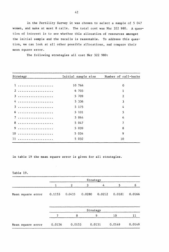
In the Fertility Survey it was chosen to select a sample of 5 047
women, and make at most 8 calls. The total cost was Nkr 322 980. A ques-
tion of interest is to see whether this allocation of resources amongst
the initial sample and the recalls is reasonable. To address this ques-
tion, we can look at all other possible allocations, and compare their
mean square error.
The following strategies all cost Nkr 322 980:
Strategy Initial sample size Number of call-backs
1 10 766 0
2 6 705 1
3 5 709 2
4 5 336 3
5 5 175 4
6 5 101 5
7 5 064 6
8 5 047 7
9 5 039 8
10 5 034 9
11 5 032 10
In table 19 the mean square error is given for all strategies.
Table 19.
Strategy
1 2 3 4 5 6
Mean square error
Mean square error
0.1155 0.0433 0.0280 0.0212 0.0181 0.0166
Strategy
7 8 9 10 11
0.0156 0.0153 0.0151 0.0149 0.0149
43
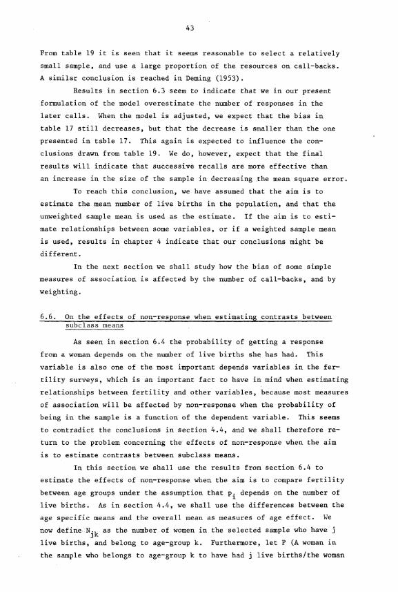
From table 19 it is seen that it seems reasonable to select a relatively
small sample, and use a large proportion of the resources on call-backs.
A similar conclusion is reached in Deming (1953).
Results in section 6.3 seem to indicate that we in our present
formulation of the model overestimate the number of responses in the
later calls. When the model is adjusted, we expect that the bias in
table 17 still decreases, but that the decrease is smaller than the one
presented in table 17. This again is expected to influence the con-
clusions drawn from table 19. We do, however, expect that the final
results will indicate that successive recalls are more effective than
an increase in the size of the sample in decreasing the mean square error.
To reach this conclusion, we have assumed that the aim is to
estimate the mean number of live births in the population, and that the
unweighted sample mean is used as the estimate. If the aim is to esti-
mate relationships between some variables, or if a weighted sample mean
is used, results in chapter 4 indicate that our conclusions might be
different.
In the next section we shall study how the bias of some simple
measures of association is affected by the number of call-backs, and by
weighting.
6.6. On the effects of non-response when estimating contrasts betweensubclass means
As seen in section 6.4 the probability of getting a response
from a woman depends on the number of live births she has had. This
variable is also one of the most important depends variables in the fer-
tility surveys, which is an important fact to have in mind when estimating
relationships between fertility and other variables, because most measures
of association will be affected by non-response when the probability of
being in the sample is a function of the dependent variable. This seems
to contradict the conclusions in section 4.4, and we shall therefore re-
turn to the problem concerning the effects of non-response when the aim
is to estimate contrasts between subclass means.
In this section we shall use the results from section 6.4 to
estimate the effects of non-response when the aim is to compare fertility
between age groups under the assumption that p i depends on the number of
live births. As in section 4.4, we shall use the differences between the
age specific means and the overall mean as measures of age effect. We
now define .Nik as the number of women in the selected sample who have j
live births, and belong to age-group k. Furthermore, let P (A woman in
the sample who belongs to age-group k to have had j live births/the woman
44
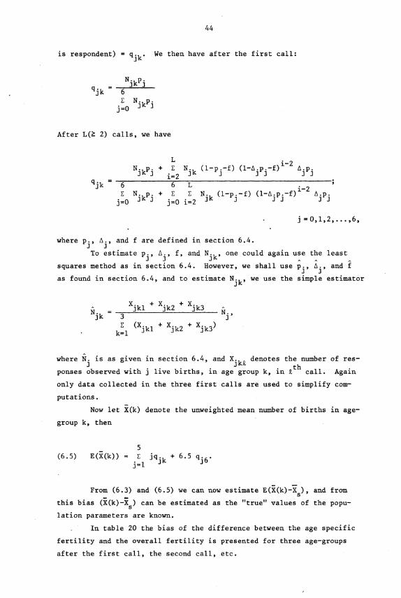
is respondent) = qjk . We then have after the first call:
q. - jk 6
E N. p.j=0 3k 3
After L(k 2) calls, we have
Ni k pi +
i=2E N.
jk (1-p.-f) (1f)
i-2 A.p.
J J J J J3
6 6 LE N.,p. + E E N., (1- .-f) (1-A.p.-f) i-2 A.p.
j=0 j=0 i=2 3' J J
j =0,1,2,•••,6,
A A A
squares method as in section 6.4. However, we shall use p., A., and fJ J
as found in section 6.4, and to estimateN .jk , we use the simple estimator
N. -jk 3 J'E+ X. )(X.j jk2 + X.jk3
k=1
Awhere N. is as given in section 6.4, andX. denotes the number of res-
Jjkk
ponses observed with j live births, in age group k, i th
n t call. Again
only data collected in the three first calls are used to simplify com-
putations.
Now let R(k) denote the unweighted mean number of births in age-
group k, then
5(6.5) E(R(k)) = E jq., + 6 . 5 q6•
j=1 3K- qj6
From (6.3) and (6.5) we can now estimate E( ii(k)--is), and from
this bias (X(k)-Xs ) can be estimated as the "true" values of the popu-
lation parameters are known.
In table 20 the bias of the difference between the age specific
fertility and the overall fertility is presented for three age-groups
after the first call, the second call, etc.
N.,Kp.3 .3
qjk
where p., A., and f are defined in section 6.4.J J
could again use the leastJ J
Njk
Xj
+ X + X.jkl k2 jk3 ^
N.
45
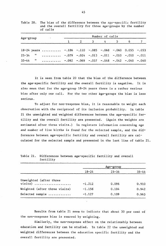
Table 20. The bias of the difference between the age-specific fertilityand the overall fertility for three age-groups by the numberof calls
Age-groupNumber of calls
1 2 3 4 5 6 7
18-24 years -.186 -.110 -.085 -.068 -.060 0.055 -.053
25-34 " -.079 -.024 -.013 -.011 -.010 -.010 -.011
35-44 " -.092 -.069 -.057 -.048 -.042 -.040 -.040
It is seen from table 20 that the bias of the difference between
the age-specific fertility and the overall fertility is negative. It is
also seen that for the age-group 18-24 years there is a rather serious
bias after only one call. For the two other Age-groups the bias is less
serious.
To adjust for non-response bias, it is reasonable to weight each
observation with the reciprocal of its inclusion probability. In table
21 the unweighted and weighted differences between the age-specific fer-
tility and the overall fertility are presented. (Again the weights are
estimated after three visits.) In registers information concerning age
and number of live births is found for the selected sample, and the dif-
ferences between age-specific fertility and overall fertility are cal-
culated for the selected sample and presented in the last line of table 21.
Table 21. Differences between age-specific fertility and overallfertility
Age-group
18-24 25-34 35-44
Unweighted (after threevisits) -1.212 0.096 0.910
Weighted (after three visits) -1.158 0.104 0.942
Selected sample -1.127 0.109 0.963
Results from table 21 seem to indicate that about 50 per cent of
the non-response bias is removed by weighting.
Similarly, the non-response effect on the relationship between
education and fertility can be studied. In table 22 the unweighted and
weighted differences between the education specific fertility and the
overall fertility are presented.

46
Table 22. Differences between education specific fertility and overallfertility
Education group
1 2 3 4 5 6 7
Unweighted (afterthree visits)
Weighted (afterthree visits)
1.203
1.234
0.673
0.701
-0.727
-0.702
0.000
0.003
-0.874
-0.853
-0.297
-0.290
-0.234
-0.231
In table 22 is seen that the difference between the weighted and
unweighted estimate is positive, indicating that the difference between
age-specific fertility and overall fertility is positive.

47
REFERENCES
Bartholomew, D.J, (1961): A Method of Allowing for "not-at-home" Biasin Sample Surveys. Applied Statistics, 1.
Deming, W.E. (1953): On a Probability Mechanism to Attain an EconomicBalance between the Resultant Error of Response and the Bias ofNon-Response. Journal of the American Statistical Association(Dec.).
Platek, R.A. (1977): Factors Affecting Non-Response. Paper presentedat the 41s t Session of the ISI, New Delhi.
Politz, A.N. and Simmons, W.R. (1949): An Attempt to get the "not-at-homes" into the sample without call-backs. J. am. stat.Assoc., 44.
Pullum, T.W. (1978): Standardization. World Fertility Survey. TechnicalBulletin, No. 3/Tech. 597.
Thomsen, I. (1971): On the Effect of Non-Response in the NorwegianElection Survey 1969. Statistisk Tidsskrift, 3.
Thomsen, I. (1973): A Note on the Efficiency of Weighting Subclass Meansto Reduce the Effects of Non-Response when Analysing Survey Data.Statistisk Tidsskrift, 11, pp. 278-285.
Zarkovich, S.S. (1966): Quality of Statistical Data, Food and AgricultureOrganisation of the United Nations, Rome.


49
Appendix 1
MAXIMUM-LIKELIHOOD ESTIMATION OF p, f, AND A
Let N denote the number of elements in the selected sample, N i
denotes the number of elements responding in the i th call, and F i denotes
the number of elements categorized as non-respondents in the ith call.
We then have that
P(N i = ni n F 1 = f l ) - Nn1
f1
(N-n1-f
1)
p f (1-p-f)n (N-n1-f1):
If i 2 we have that
i-1 i-1
P(N. = n.f1F=f1r1N. = n., fl F. = f,) =j=1 J J j=1 J 1
n. f. N- E n. - E f .
(A.1.) k(p) 1 f 1 (l-Ap-f) j =1 j j=1
where k- is a constant independent of p, f, and A. Assume that at most
j calls have been made, then
P( n (N. = n. n F. = f.)) =i=1 1111
3-1= P(N. = n.f1F. = f. 1 n (N. = n. n F. = f.)) •
j j ji=11 I.
3-2• P(N. = n. n F. = f. 1 n (N. = n. n F. = f.)) •
j-1 j-1 j-1 j-1 .1=1
(A.2.) • P(N2 = n2 n F2 = f 2 IN 1 = n1 flF 1 = f 1 ) p(Ni = n1 flF 1 = f1).

50
From (A.1) and (A.2) follows that
P( n (N. = n.11 F. = f.)) =i=l iiii
jj f
jiE n. E (j-1)N- (-1)(n
1+f
1)- E (j-i+1)
= 7T ki(Ap)1=2 1
f1=1
(1-Ap-f)i=2
i=1
n1N-n
1-f
1• p (1-p - f)
ni N-n1-f
1= 7TyAp) afb(io cp L u_p_f)
i=177-k h(p,f,A),
i=1 1
j jwhere a = E n., b = E f., and
i=2 1 i=1 1
jc = (j-1) N-(-1)(n
1+f
1) - E (j-i+1)(n.+f.).
i=2
Furthermore,
in h(p,f,A) = amp + alnA + blnf +
+ c1n(1-Ap-f) + n1 lnp + (N-n1-f 1 )ln(1-p-f)
After derivation with respect to p, A, and f the following equa-
tions must be fulfilled to maximize h(p,f,A).
n N-n-fA3
a ln h a Ac + 1 1 1 (..) - - - - 0
D p p 1 - Ap - f p 1-p - f
(A4 ln h a cp-0.). - -
DA A 1 - Ap - f
N-n1
- f1 3 ln h b c (A.5.) - 0D f f 1-Ap-f 1-p-f

51
The maximum-likelihood estimators are now found from (A.3) - (A.5)
E F.
-
b i=1 N -F 1 + a+b+c j
N1 (14)-
P - N-F 1
- a(14) A -A
p(a+c)
to be
and
j N - E (j-1)(Fi
+Ni
)1=1
52
Utkommet i serien ART
Issued in the series Articles from the Central Bureau of Statistics (ART)
Nr. 111 Jon Blaalid og Øystein Olsen: Etterspørsel etter energiEn litteraturstudie The Demand for Energy A Survey 197876 s. kr 11,00 ISBN 82-537-0892-0
" 112 Inger Gabrielsen: Aktuelle skattetall 1978 Current Tax Data1978 55 s. kr 9,00 ISBN 82-537-0896-3
" 113 Gunvor Iversen: Skiftarbeid Shift Work 1979 72 s. kr 11,00ISBN 82-537-0915-3
" 114 Vidar Christiansen og Eilev S. Jansen: Implicit Social Prefe-rences in the Norwegian System of Indirect Taxation Implisittevelferdsvurderinger i det norske systemet av indirekte skatter1979 36 s. kr 9,00 ISBN 82-537-0935-8
" 115 Hallstein Myklebost: Bosetningsutviklingen i Norge 1960 - 1970Population and Settlement Change in Norway 1979 95 s.kr 11,00 ISBN 82-537-0946-3
" 116 Helge Brunborg: Cohabitation without Marriage in Norway Samlivuten vigsel i Norge 1979 30 s. kr 9,00 ISBN 82-537-0955-2
" 117 Odd Aukrust: Econometric Methods in Short-term Planning: TheNorwegian Lesson Økonometriske metoder i korttidsplanleggingen:Erfaringer fra Norge 1979 84 s. kr 9,00 ISBN 82-537-0963-3
" 118 Lorents Lorentsen, Steinar Strøm og Lars Erik Østby: Virkningenpå norsk øknomi av en pause i den videre kraftutbyggingImpacts on the Norwegian Economy of a Temporary Halt in theGrowth of Electricity Supply 1979 36 s. kr 9,00ISBN 82-537-0984-6
" 119 Jan MOnnesland: Analytisk glatting av rater for første gangsgiftermål Analytic Graduation of First Time Nuptiality Rates1979 38 s. kr 9,00 ISBN 82-537-1008-9
" 121 Ib Thomsen og Erling Siring: On the Causes and Effects of Non-Response. Norwegian Experiences Om årsakene til og virkningeneav frafall. Erfaringer fra Norge 1980 52 s. kr 11,00ISBN 82-537-1107-7
Fullstendig oversikt over tidligere nummer av serien Artikler finnes inr. 120.

Publikasjonen utgis i kommisjon hosH. Aschehoug & Co. og Universitetsforlaget, Oslo,
og er til salgs hos alle bokhandlerePris kr 11,00
Omslag trykt hos Grondahl 8z Son Trykkeri, Oslo
ISBN 82-537-1107-7ISSN 0085-431x