R&S 15. Estuarine systems of the South American region: carbon, nitrogen and phosphorus fluxes

LAND-OCEAN INTERACTIONS IN THE COASTAL ZONE (LOICZ)Core Project of the

International Geosphere-Biosphere Programme: A Study of Global Change (IGBP)

and

UNITED NATIONS ENVIRONMENT PROGRAMME (UNEP)Supported by the Global Environment Facility (GEF)

ESTUARINE SYSTEMS OF THE SOUTH AMERICAN REGION: CARBON,NITROGEN AND PHOSPHORUS FLUXES

Compiled and edited by V. Dupra, S.V. Smith, J.I. Marshall Crossland and C.J. Crossland

LOICZ REPORTS & STUDIES No. 15

ESTUARINE SYSTEMS OF THE SOUTH AMERICAN REGION: CARBON,NITROGEN AND PHOSPHORUS FLUXES

V. Dupra & S.V. SmithSchool of Ocean and Earth Science and Technology

Honolulu, Hawaii, USA

J.I. Marshall Crossland & C.J. CrosslandLOICZ International Project Office

Texel, The Netherlands

United Nations Environment ProgrammeSupported by financial assistance from the Global Environment Facility

LOICZ REPORTS & STUDIES NO. 15

Published in the Netherlands, 2000 by:LOICZ International Project OfficeNetherlands Institute for Sea ResearchP.O. Box 591790 AB Den Burg - TexelThe NetherlandsEmail: [email protected]

The Land-Ocean Interactions in the Coastal Zone Project is a Core Project of the “International Geosphere-Biosphere Programme: A Study Of Global Change” (IGBP), of the International Council of Scientific Unions.

The LOICZ IPO is financially supported through the Netherlands Organisation for Scientific Research by: theMinistry of Education, Culture and Science (OCenW); the Ministry of Transport, Public Works and WaterManagement (V&W RIKZ); and by The Royal Netherlands Academy of Sciences (KNAW), and TheNetherlands Institute for Sea Research (NIOZ).

This report and allied workshops are contributions to the United Nations Environment Programme project: TheRole of the Coastal Ocean in the Disturbed and Undisturbed Nutrient and Carbon Cycles (Project Number GF1100-99-07), financially supported by the Global Environment Facility, and being implemented by LOICZ.

COPYRIGHT 2000, Land-Ocean Interactions in the Coastal Zone Core Project of the IGBP.

Reproduction of this publication for educational or other, non-commercial purposes isauthorised without prior permission from the copyright holder.

Reproduction for resale or other purposes is prohibited without the prior, written permission ofthe copyright holder.

Citation: Smith, S.V., V. Dupra, J.I. Marshall Crossland and C.J. Crossland 2000 Estuarine systems ofthe South American region: carbon, nitrogen and phosphorus fluxes. LOICZ Reports & StudiesNo. 15, ii + 87 pages, LOICZ, Texel, The Netherlands.

ISSN: 1383-4304

Cover: The cover shows an image of South America (GTOPO30 elevation map), with the budgetedestuaries circled.

Disclaimer: The designations employed and the presentation of the material contained in this report do notimply the expression of any opinion whatsoever on the part of LOICZ, the IGBP or UNEPconcerning the legal status of any state, territory, city or area, or concerning the delimitationsof their frontiers or boundaries. This report contains the views expressed by the authors andmay not necessarily reflect the views of the IGBP or UNEP.

_________________________________

The LOICZ Reports and Studies Series is published and distributed free of charge to scientists involved inglobal change research in coastal areas.

i

TABLE OF CONTENTS Page

1. OVERVIEW OF WORKSHOP AND BUDGETS RESULTS

2. BRAZIL COASTAL SYSTEMS

2.1 Rio Sergipe Estuary, Sergipe StateMarcelo F. Landim de Souza

2.2 Piaui River Estuary, Sergipe StateMarcelo F. Landim de Souza, V.R. Gomes, S.S. de Freitas, R.C.B.Andrade, B.A. Knoppers and S.V. Smith

2.3 Marica-Guarapina coastal lagoons, Rio de Janeiro StateErminda da C.G. Couto, N.A.C. Zyngier, V.R. Gomes, B.A. Knoppersand M.F. Landim de Souza

2.4 Piratininga-Itaipu coastal lagoons, Rio de Janeiro StateErminda da C.G. Couto, N.A.C. Zyngier and M.F. Landim de Souza

2.5 Paranagua Bay estuarine complex, Parana StateE. Marone, Eunice C. Machado, R.M. Lopes and E.T. Silva

2.6 Camboriu River Estuary, Santa Catarina StateJurandir Pereira Filho and C.A. Schettini

2.7 Araruama Lagoon, Rio de Janeiro State – a hypersaline lagoonal systemWeber F. Landim de Souza and B.A. Knoppers

3. URUGUAY ESTUARINE SYSTEMS3.1 The Frontal Zone of the Rio de la Plata

Gustavo J. Nagy

4. ARGENTINA ESTUARINE SYSTEMS4.1 Bahia Nueva, Golfo Nuevo, Patagonia

Monica N. Gil and J.L. Esteves

5. ECUADOR ESTUARINE SYSTEMS5.1 Gulf of Guayaquil

Isabel Tutiven U.

6. CHILE ESTUARINE SYSTEMS6.1 Aysen Sound

Nelson Silva S., Dafne Guzman Z. and Alexander Veldenegro M.

7. REFERENCES

1

6

6

10

18

22

26

33

37

4040

4444

5151

5555

65

ii

APPENDICESAppendix I CABARET – Laura T. David

Appendix II Typology and Budgets/Budget Sites Information – Robert W.Buddemeier

Appendix III Workshop Report

Appendix IV Participants and Contributing Authors

Appendix V Agenda

Appendix VI Terms of Reference

Appendix VII Glossary

Note: Where there is more than one author, the underlined name indicates theworkshop participant.

Page7070

76

78

80

83

85

87

1

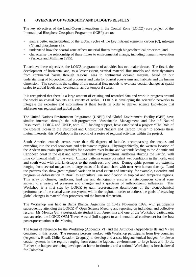
1. OVERVIEW OF WORKSHOP AND BUDGETS RESULTS

The key objectives of the Land-Ocean Interactions in the Coastal Zone (LOICZ) core project of theInternational Biosphere-Geosphere Programme (IGBP) are to:

• gain a better understanding of the global cycles of the key nutrient elements carbon (C), nitrogen(N) and phosphorus (P);

• understand how the coastal zone affects material fluxes through biogeochemical processes; and• characterise the relationship of these fluxes to environmental change, including human intervention

(Pernetta and Milliman 1995).

To achieve these objectives, the LOICZ programme of activities has two major thrusts. The first is thedevelopment of horizontal and, to a lesser extent, vertical material flux models and their dynamicsfrom continental basins through regional seas to continental oceanic margins, based on ourunderstanding of biogeochemical processes and data for coastal ecosystems and habitats and the humandimension. The second is the scaling of the material flux models to evaluate coastal changes at spatialscales to global levels and, eventually, across temporal scales.

It is recognised that there is a large amount of existing and recorded data and work in progress aroundthe world on coastal habitats at a variety of scales. LOICZ is developing the scientific networks tointegrate the expertise and information at these levels in order to deliver science knowledge thataddresses our regional and global goals.

The United Nations Environment Programme (UNEP) and Global Environment Facility (GEF) havesimilar interests through the sub-programme: “Sustainable Management and Use of NaturalResources”. LOICZ and UNEP, with GEF funding support, have established a project: “The Role ofthe Coastal Ocean in the Disturbed and Undisturbed Nutrient and Carbon Cycles” to address thesemutual interests; this Workshop is the second of a series of regional activities within the project.

South America extends across more than 65 degrees of latitude, encompassing the tropics andextending into the cool temperate and subantarctic regions. Physiographically, the western location ofthe Andean mountain spine provides for extensive river basins and wetlands leading to the Atlantic andCaribbean coast in the east and north, and relatively precipitous landforms abutting the Pacific, withlittle continental shelf to the west. Climate patterns ensure prevalent wet conditions in the north, eastand south-west with arid landscapes to the south-east and west. Demographic patterns are extreme,ranging from several megacities to large tracts of land and shore with near-zero human density. Landuse patterns also show great regional variation in areal extent and intensity, for example, extensive andprogressive deforestation in Brazil to agricultural use modification in tropical and temperate regions.This array of climate, landforms, land use and demography ensures a heterogeneous coastal zonesubject to a variety of pressures and changes and a spectrum of anthropogenic influences. ThisWorkshop is a first step by LOICZ to gain representative descriptions of the biogeochemicalperformance of the coastal zone ecosystems within the region, in order to address the goals of assessingglobal changes in material flux processes and the human dimension.

The Workshop was held in Bahia Blanca, Argentina on 10-12 November 1999, with participantssubsequently attending the LOICZ 4th Open Science Meeting and reporting on individual and collectiveresults. Ms Monica Gil, a postgraduate student from Argentina and one of the Workshop participants,was awarded the LOICZ OSM Travel Award (full support to an international conference) for the bestposter/presentation at the Meeting.

The terms of reference for the Workshop (Appendix VI) and the Activities (Appendices III and V) arecontained in this report. The resource persons worked with Workshop participants from five countries(Argentina, Brazil, Chile, Ecuador, Uruguay) to develop and assess biogeochemical budgets for elevencoastal systems in the region, ranging from estuarine lagoonal environments to large bays and fjords.Further site budgets are being developed at home institutions and a national Workshop is foreshadowedfor Colombia.

2

GuayaquilGulf

AysenSound

SergipeEstuary

Marica-GuarapinaLagoons

Bahliaa Nueva

ParanaguaBay

Rio delaPlata

CamboriuBight

Piaui

AraruamaLagoon

Piratinga-ItaipuLagoons

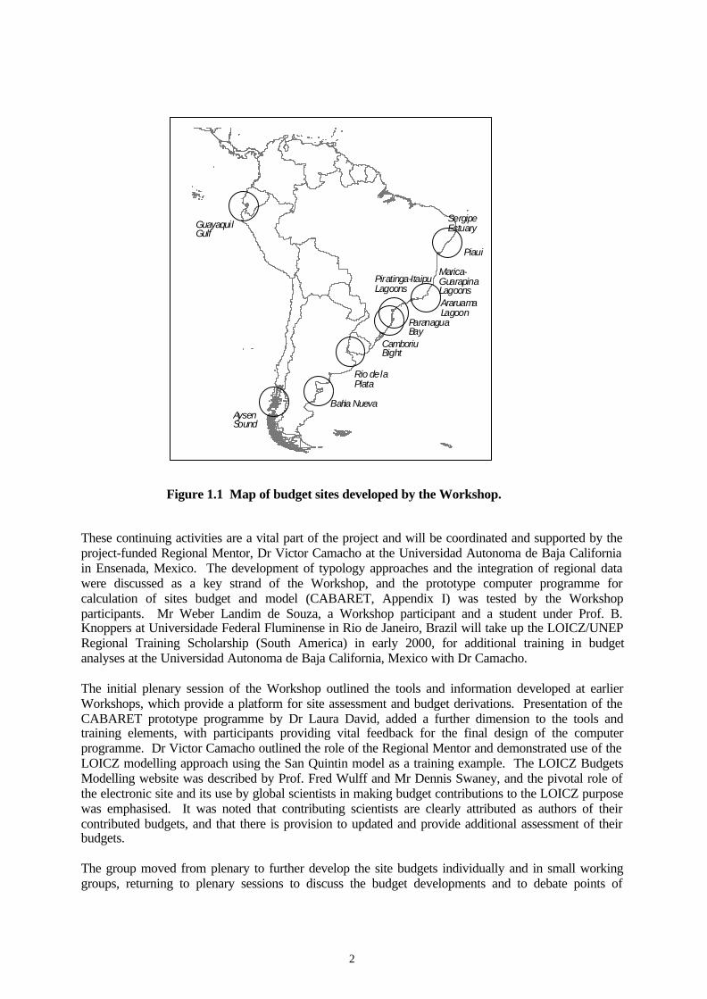
Figure 1.1 Map of budget sites developed by the Workshop.

These continuing activities are a vital part of the project and will be coordinated and supported by theproject-funded Regional Mentor, Dr Victor Camacho at the Universidad Autonoma de Baja Californiain Ensenada, Mexico. The development of typology approaches and the integration of regional datawere discussed as a key strand of the Workshop, and the prototype computer programme forcalculation of sites budget and model (CABARET, Appendix I) was tested by the Workshopparticipants. Mr Weber Landim de Souza, a Workshop participant and a student under Prof. B.Knoppers at Universidade Federal Fluminense in Rio de Janeiro, Brazil will take up the LOICZ/UNEPRegional Training Scholarship (South America) in early 2000, for additional training in budgetanalyses at the Universidad Autonoma de Baja California, Mexico with Dr Camacho.

The initial plenary session of the Workshop outlined the tools and information developed at earlierWorkshops, which provide a platform for site assessment and budget derivations. Presentation of theCABARET prototype programme by Dr Laura David, added a further dimension to the tools andtraining elements, with participants providing vital feedback for the final design of the computerprogramme. Dr Victor Camacho outlined the role of the Regional Mentor and demonstrated use of theLOICZ modelling approach using the San Quintin model as a training example. The LOICZ BudgetsModelling website was described by Prof. Fred Wulff and Mr Dennis Swaney, and the pivotal role ofthe electronic site and its use by global scientists in making budget contributions to the LOICZ purposewas emphasised. It was noted that contributing scientists are clearly attributed as authors of theircontributed budgets, and that there is provision to updated and provide additional assessment of theirbudgets.

The group moved from plenary to further develop the site budgets individually and in small workinggroups, returning to plenary sessions to discuss the budget developments and to debate points of

3

approach and interpretation. Eleven budgets were developed during the Workshop (Figure 1.1, Table1.1), with two additional sites in Chile and further sites in Brazil and Argentina in progress.

The common element in the budget descriptions is the use of the LOICZ approach to budgetdevelopment, which allows for global comparisons and application of the typology approach. Thedifferences in the descriptive presentations reflect the variability in richness of site data, the complexityof the sites and processes, and the extent of detailed process understanding for the sites. Supportinformation for the various estuarine locations, describing the physical environmental conditions andrelated forcing functions including the history and potential anthropogenic pressure, is an importantpart of the budget information for each site. These budgets, data and their wider availability inelectronic form (CD-ROM, LOICZ website) will provide opportunity for further assessment,comparisons and potential use with wider scales of patterns in system response and human pressures.

The budget information for each site is discussed individually and reported in units that are convenientfor that system (either as daily or annual rates). To provide for an overview and ease of comparison,the key data are presented in an “annualised” form and nonconservative fluxes are reported per unitarea (Tables 1.1 and 1.2).

Key outcomes and findings from the Workshop include:

1. A set of eleven budgets representing a range of coastal settings for the South American region –estuaries, coastal lagoons, large embayments and fjords. These budgets provide insights intoseasonality, influence of human activities as drivers of change and sensitivity of systemperformance to nutrients derived from land and ocean. Further development of a number of thesebudgets and additional site models are foreshadowed by participants and through the activity of theRegional Mentor. It is expected that additional models will add to “replication” of system typesand support further trend analyses of climatic and human forcings on biogeochemical processesacross the continent and globally.

2. A variety of site examples and different measurement/data types which show approaches that canbe taken under the LOICZ Modelling protocol for first-order evaluation of net metabolism ofcoastal systems and modelling to meet LOICZ global change goals and UNEP project objectives.

3. The two coastal lagoon systems (Marica-Guarapina, Piratininga-Itaipu) were used for analysis ofthe net metabolism trends and trophic changes within component parts of the water continuum,from land through the lagoon systems to the sea. Seasonal forcing (wet and dry seasons) wereconsidered along with different stoichiometric ratios in the calculation of net metabolism values.

4. The estuarine systems (Rio Sergipe, Paranagua Bay), modelled as multiple horizontal boxes,indicated seasonal variations in net autotrophy/heterotrophy and nitrogen fixation/denitrificationoccurring horizontally within the systems. Further refinement of the budgets and additional siteswith similar settings will assist in evaluating these variations.

5. The fjord site (Aysen Sound) provided a model of a deep stratified system, with evidence ofmarked inter-annual variability in surface water net metabolism. Further understanding of the netmetabolic patterns of the full system will depend on gaining summer (and a wider seasonal spreadof) physico-chemical data.

6. A new tool (CABARET) is nearing final development which will provide user-friendly computer-assisted assessment of material fluxes in estuarine systems following the LOICZ Modellingapproach.

The Workshop was hosted by the Instituto Argentino de Oceanografia in Bahia Blanca, Argentina.LOICZ is grateful for this support and indebted to Dr Gerardo Perillo and Institute staff, and to theWorkshop resource scientists for their contributions to the success of the Workshop. LOICZ gratefullyacknowledges the effort and work of the participants not only for their significant contributions to theWorkshop goals, but also for their continued interaction beyond the meeting activities.

4

The Workshop and this report are contributions to the GEF-funded UNEP project: The Role of theCoastal Ocean in the Disturbed and Undisturbed Nutrient and Carbon Cycles, recently establishedwith LOICZ and contributing to the UNEP sub-programme: Sustainable Management and Use ofNatural Resources.

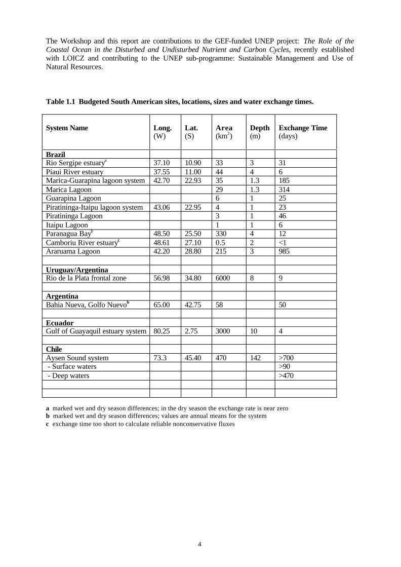
Table 1.1 Budgeted South American sites, locations, sizes and water exchange times.

System Name Long.(W)

Lat.(S)

Area(km2)

Depth(m)

Exchange Time(days)

BrazilRio Sergipe estuarya 37.10 10.90 33 3 31Piaui River estuary 37.55 11.00 44 4 6Marica-Guarapina lagoon system 42.70 22.93 35 1.3 185Marica Lagoon 29 1.3 314Guarapina Lagoon 6 1 25Piratininga-Itaipu lagoon system 43.06 22.95 4 1 23Piratininga Lagoon 3 1 46Itaipu Lagoon 1 1 6Paranagua Bayb 48.50 25.50 330 4 12Camboriu River estuaryc 48.61 27.10 0.5 2 <1Araruama Lagoon 42.20 28.80 215 3 985

Uruguay/ArgentinaRio de la Plata frontal zone 56.98 34.80 6000 8 9

ArgentinaBahia Nueva, Golfo Nuevob 65.00 42.75 58 50

EcuadorGulf of Guayaquil estuary system 80.25 2.75 3000 10 4

ChileAysen Sound system 73.3 45.40 470 142 >700 - Surface waters >90 - Deep waters >470

a marked wet and dry season differences; in the dry season the exchange rate is near zerob marked wet and dry season differences; values are annual means for the systemc exchange time too short to calculate reliable nonconservative fluxes

5

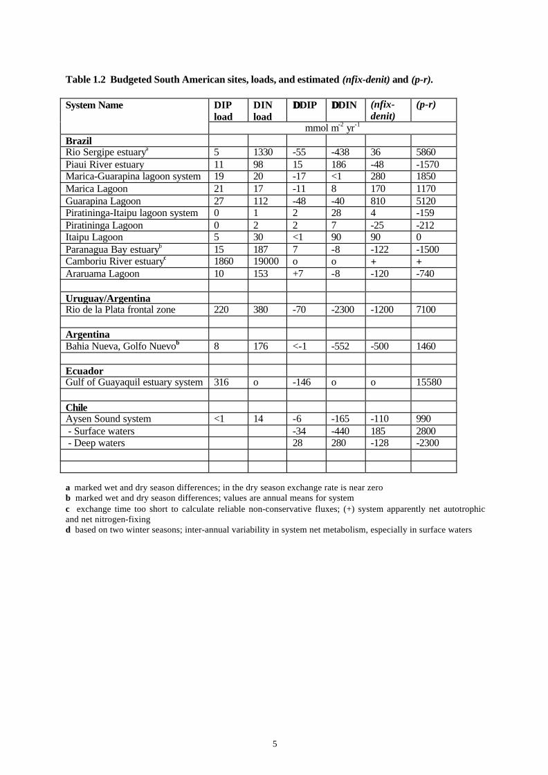
Table 1.2 Budgeted South American sites, loads, and estimated (nfix-denit) and (p-r).

DIPload

DINload

∆∆DIP ∆∆DIN (nfix-denit)

(p-r)System Name

mmol m-2 yr-1

BrazilRio Sergipe estuarya 5 1330 -55 -438 36 5860Piaui River estuary 11 98 15 186 -48 -1570Marica-Guarapina lagoon system 19 20 -17 <1 280 1850Marica Lagoon 21 17 -11 8 170 1170Guarapina Lagoon 27 112 -48 -40 810 5120Piratininga-Itaipu lagoon system 0 1 2 28 4 -159Piratininga Lagoon 0 2 2 7 -25 -212Itaipu Lagoon 5 30 <1 90 90 0Paranagua Bay estuaryb 15 187 7 -8 -122 -1500Camboriu River estuaryc 1860 19000 o o + +Araruama Lagoon 10 153 +7 -8 -120 -740

Uruguay/ArgentinaRio de la Plata frontal zone 220 380 -70 -2300 -1200 7100

ArgentinaBahia Nueva, Golfo Nuevob 8 176 <-1 -552 -500 1460

EcuadorGulf of Guayaquil estuary system 316 o -146 o o 15580

ChileAysen Sound system <1 14 -6 -165 -110 990 - Surface waters -34 -440 185 2800 - Deep waters 28 280 -128 -2300

a marked wet and dry season differences; in the dry season exchange rate is near zerob marked wet and dry season differences; values are annual means for systemc exchange time too short to calculate reliable non-conservative fluxes; (+) system apparently net autotrophicand net nitrogen-fixingd based on two winter seasons; inter-annual variability in system net metabolism, especially in surface waters

6

BRAZIL COASTAL SYSTEMS

2.1 Rio Sergipe, Sergipe State

Marcelo F. Landim de Souza

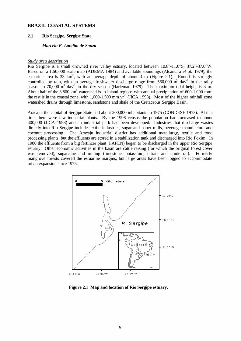
Study area descriptionRio Sergipe is a small drowned river valley estuary, located between 10.8°-11.0°S, 37.2°-37.0°W.Based on a 1:50,000 scale map (ADEMA 1984) and available soundings (Alcântara et al. 1979), theestuarine area is 33 km2, with an average depth of about 3 m (Figure 2.1). Runoff is stronglycontrolled by rain, with an average freshwater discharge range from 560,000 m3 day-1 in the rainyseason to 70,000 m3 day-1 in the dry season (Harleman 1979). The maximum tidal height is 3 m.About half of the 3,800 km2 watershed is in inland regions with annual precipitation of 600-1,000 mm;the rest is in the coastal zone, with 1,000-1,500 mm yr-1 (JICA 1998). Most of the higher rainfall zonewatershed drains through limestone, sandstone and shale of the Cretaceous Sergipe Basin.

Aracaju, the capital of Sergipe State had about 200,000 inhabitants in 1975 (CONDESE 1973). At thattime there were few industrial plants. By the 1996 census the population had increased to about400,000 (JICA 1998) and an industrial park had been developed. Industries that discharge wastesdirectly into Rio Sergipe include textile industries, sugar and paper mills, beverage manufacture andcoconut processing. The Aracaju industrial district has additional metallurgy, textile and foodprocessing plants, but the effluents are stored in a stabilization tank and discharged into Rio Poxim. In1980 the effluents from a big fertilizer plant (FAFEN) began to be discharged in the upper Rio Sergipeestuary. Other economic activities in the basin are cattle raising (for which the original forest coverwas removed), sugarcane and mining (limestone, potassium, nitrate and crude oil). Formerlymangrove forests covered the estuarine margins, but large areas have been logged to accommodateurban expansion since 1975.

R . S e rg ipe

37 .1 0 °W 3 7 .0 5 °W 3 7 .0 0 °W

10 .9 0 °S

1 0 .9 5 °S

11 .0 0 ° S

0 5 Ki lom et e rs

R . S e rg ip e

B r a z il

Figure 2.1 Map and location of Rio Sergipe estuary.

7

For a preliminary salt, water and dissolved nutrients budget, the early data available in Alcântara et al.(1979) for June and October 1975 were used. Evaporation and precipitation data were obtained fromIESAP (1988) and mean freshwater discharges from Harleman (1979). The anthropogenic input wasestimated from a per capita index of 9.5 moles inorganic P person yr-1 and 140 moles inorganic Nperson yr-1 (S.V. Smith, personal communication). Using a population of about 200,000 persons in1975 results in approximate waste loads of about 5,000 mol DIP d-1 and 80,000 mol DIN d-1.

Water and salt balanceAs true oceanic data were not available, the outer part of the estuary was used for the “ocean” and onlythe inner part was budgeted (Figure 2.1). The present one-dimensional budget should be checkedfurther against two-dimensional procedures, since some stratification was observed, especially in theouter sampling stations.

The difference between hydraulic (Vsyst/|VR|) residence time and total water exchange time(Vsyst/(|VR|+VX)) indicates the efficiency of tidal mixing. Water exchange times were high, due to thelow freshwater discharge (Figures 2.2 and 2.3). A slightly positive water balance in the dry seasonindicates a small residual outflow from the estuary, compared with the balance in the rainy season. Inthe dry season, the estuary is “plugged”, with effectively infinite exchange time. Tidal mixing is themain water flow in both seasons.

DIP and DIN balanceThe only dissolved nutrients for which data are available are nitrate (considered as a lower estimate ofDIN) and dissolved inorganic phosphorus (DIP). In fact, DIP was below the detection limit in thesampling dates of this budget (Alcântara et al. 1979). Although unusual, these results agree with thoseobtained in a 1999 sampling (unpublished data), in which most samples also had DIP below detectionlimits, despite the greatly increased anthropogenic loading. To allow further stoichiometric linking, itwas assumed that all anthropogenic contribution was removed from water column, resulting in ∆DIP ≅-5x103 mol day-1. Given the very long water exchange time, this is not an unreasonable scenario. Thisleads to the “stoichiometric conclusion” that the estuary is a net autotrophic system.

Dissolved inorganic nitrogen budgets (Figures 2.4 and 2.5) indicate ∆DIN ranging from -66x103 molday-1 in the rainy season to -87x103 mol day-1 in the dry season. In the rainy season (Figure 2.4) morethan 50% of DIN inputs were exported to the outer reaches, while in the dry season the export was onlyabout 1% (Figure 2.5).

Thus, this estuary acts as an effective sink of DIP and DIN, especially during the dry season.

It must be emphasized that the extremely low DIP concentrations and high DIN concentrations appearto be very unusual conditions.

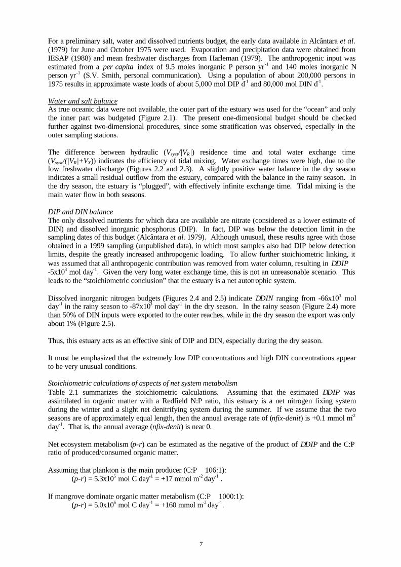
Stoichiometric calculations of aspects of net system metabolismTable 2.1 summarizes the stoichiometric calculations. Assuming that the estimated ∆DIP wasassimilated in organic matter with a Redfield N:P ratio, this estuary is a net nitrogen fixing systemduring the winter and a slight net denitrifying system during the summer. If we assume that the twoseasons are of approximately equal length, then the annual average rate of (nfix-denit) is +0.1 mmol m-2

day-1. That is, the annual average (nfix-denit) is near 0.

Net ecosystem metabolism (p-r) can be estimated as the negative of the product of ∆DIP and the C:Pratio of produced/consumed organic matter.

Assuming that plankton is the main producer (C:P ≅ 106:1):(p-r) = 5.3x105 mol C day-1 = +17 mmol m-2 day-1 .

If mangrove dominate organic matter metabolism (C:P ≅ 1000:1):(p-r) = 5.0x106 mol C day-1 = +160 mmol m-2 day-1.

8

There is, of course, no seasonal signal, since the calculations are based on the assumption that all wasteload is taken up. The net uptake of DIP indicates that the system is apparently net autotrophic, withconsiderable uncertainty in the magnitude of this autotrophy because of the apparent importance ofmangroves in the system.

Table 2.1 Summary of stoichiometric calculations for Rio Sergipe.

Season ∆DIP ∆DINobs ∆DINexp (nfix-denit)

(p-r)plank1 (p-r)mang

2

Winter (rainy) 103 mol day-1 -5 -66 -80 +14 +530 +5,000 mmol m-2 day-1 -0.15 -1.9 -2.4 +0.4 +16 +152

Spring (dry) 103 mol day-1 -5 -87 -80 -7 +530 +5,000 mmol m-2 day-1 -0.15 -0.5 -2.4 -0.2 +16 +152

Annual average 103 mol day-1 -5 -77 -80 +3 +530 +5,000 mmol m-2 day-1 -0.15 -1.2 -2.4 +0.1 +16 +152

1Assuming a C:P ratio of 106:1 for plankton-based particulate material.2Assuming a C:P ratio of 1,000:1 for mangrove-based particulate material.

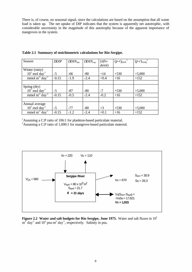
Figure 2.2 Water and salt budgets for Rio Sergipe, June 1975. Water and salt fluxes in 103

m3 day-1 and 103 psu-m3 day-1, respectively. Salinity in psu.

Sergipe River

Vsyst = 80 x 10 m Ssyst = 21.7

τ τ = 31 days

VP = 220 VE = 110

VQ1 = 560 VR = 670

Socn = 30.9

SR = 26.3

VX(Socn-Ssyst) = -VRSR = 17,621 VX = 1,915

6 3

9

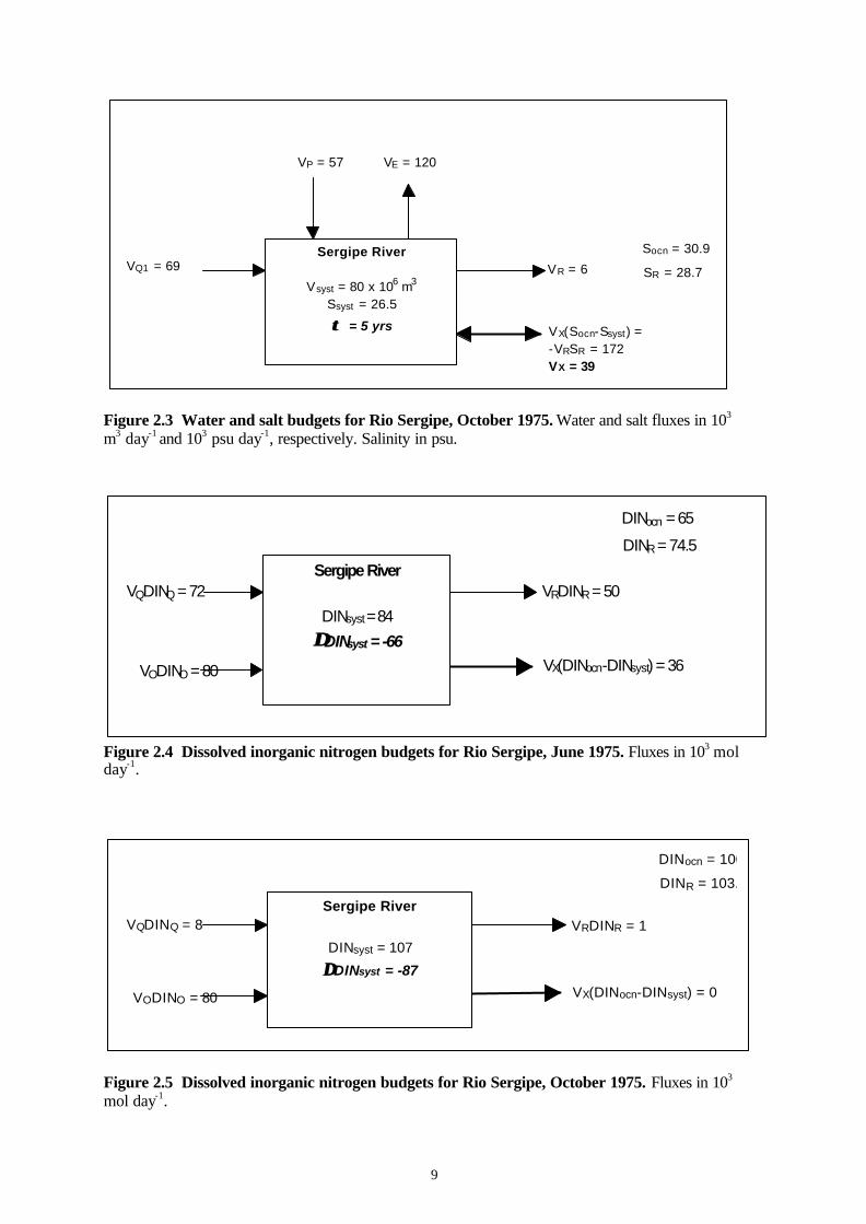
Figure 2.3 Water and salt budgets for Rio Sergipe, October 1975. Water and salt fluxes in 103

m3 day-1 and 103 psu day-1, respectively. Salinity in psu.

Figure 2.4 Dissolved inorganic nitrogen budgets for Rio Sergipe, June 1975. Fluxes in 103 molday-1.

Figure 2.5 Dissolved inorganic nitrogen budgets for Rio Sergipe, October 1975. Fluxes in 103

mol day-1.

Sergipe River

DINsyst = 84

∆∆DINsyst = -66

VQDINQ = 72 VRDINR = 50

DINocn = 65

DINR = 74.5

VX(DINocn-DINsyst) = 36VODINO = 80

Sergipe River

DINsyst = 107

∆∆DINsyst = -87


DINocn = 100

DINR = 103.5


Sergipe River

Vsyst = 80 x 10 m Ssyst = 26.5

τ τ = 5 yrs

VP = 57 VE = 120

VQ1 = 69 VR = 6

Socn = 30.9

SR = 28.7

VX(Socn-Ssyst) = -VRSR = 172 VX = 39

6 3

10

2.2 Piauí River Estuary, Sergipe State.

Marcelo F. Landim de Souza, V.R. Gomes, S.S. de Freitas, R.C.B Andrade, B.A. Knoppersand S.V. Smith

Study area descriptionThe Piauí River watershed in northern Brazil (10.5o-11.5o S, 37.2o-38.1o W, Figure 2.6) covers 4,220km2 of a geologically complex and heterogeneous terrain. An elevation of 100 m occurs between 10-20 km from the coast, and the river originates at an elevation of about 450 m. Coastal areas have awarm humid to sub-humid climate (~1,400 mm yr-1), with 1-3 dry months (“summer-spring”), whilethe inland areas have Mediterranean to dry climate (<750 mm yr-1), with 4-6 dry months. Annualprecipitation varies considerably from this average (UFS 1979). Most of the original vegetation in thebasin has been removed to allow extensive cattle raising and crops (citrus fruits, tobacco and cotton).In the coastal zone, mangrove forests are being logged and replaced by coconut plantations.

The Piauí, Piauitinga, Fundo and Guararema rivers are the main tributaries (Figure 2.6). In all of thesewatersheds there are problems due to deforestation, improper soil use, riparian wood cutting and waterpollution (JICA 1998). There is further degradation in the Piauitinga River, near the city of Estância.That river receives effluents from textile industries and high organic loading from citrus juice/foodprocessing and untreated sewage. The resulting changes in water chemistry lead the river toward netheterotrophy, denitrification and also nitrogen loss to the atmosphere as ammonia (Andrade et al.1998).

Figure 2.6 Piauí River drainage basin.

11

The entire estuary is a small drowned river valley, about 35 km long, 44 km2 in area, and with anaverage depth of 4 m (Figure 2.7). The estuary has semidiurnal tides, with a maximum spring rangeof 3 m (Souza 1999). Direct pollution discharge into the estuarine zone is almost absent, but theestuary receives anthropogenic organic loading from the Piauitinga River, as described above. Waterflow is regulated through two small reservoirs. Anthropogenic influence on dissolved inorganicnutrient concentrations is restricted to the upper Piauí River estuarine zone (Gomes et al. 1998). TheFundo River is essentially unpolluted, although it has a degraded watershed. The estuarine zone ofthese rivers has extensive mangrove coverage, though subject to increasing deforestation. There is aseaweed bank in the confluence of the Piauí and Real rivers (the prevailing taxon is Halodule sp., withsome calcareous algae Acetabularia sp.). The small phytoplankton population of the turbid waters isdominated by diatoms.

Figure 2.7 Map of Piaui River estuary, with location of sampling points.Mangrove forests are represented as dark gray areas.

Measurements of community metabolism suggest that the system is heterotrophic on an annual basis,but with occasional episodes of net autotrophy, especially in the lower estuary (Souza 1999). Theresulting loss of carbon dioxide to the atmosphere was estimated to be 4.3x108 mol yr-1. That studyalso reported that planktonic net metabolism is approximately neutral, while most of the heterotrophyoccurs in benthic and intertidal mangrove areas. However, previous work has revealed that systemmetabolism is subject to drastic short-term changes (Souza and Couto 1999).

12

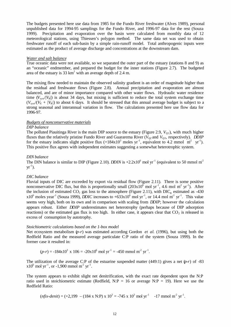
The budgets presented here use data from 1985 for the Fundo River freshwater (Alves 1989), personalunpublished data for 1994-95 samplings for the Fundo River, and 1996-97 data for the rest (Souza1999). Precipitation and evaporation over the basin were calculated from monthly data of 12meteorological stations, using Thiessen’s polygon method. The same data set was used to obtainfreshwater runoff of each sub-basin by a simple rain-runoff model. Total anthropogenic inputs wereestimated as the product of average discharge and concentrations at the downstream dam.

Water and salt balanceTrue oceanic data were not available, so we separated the outer part of the estuary (stations 8 and 9) asan “oceanic” endmember, and prepared the budget for the inner stations (Figure 2.7). The budgetedarea of the estuary is 33 km2 with an average depth of 2.4 m.

The mixing flow needed to maintain the observed salinity gradient is an order of magnitude higher thanthe residual and freshwater flows (Figure 2.8). Annual precipitation and evaporation are almostbalanced, and are of minor importance compared with other water flows. Hydraulic water residencetime (Vsyst/|VR|) is about 34 days, but mixing is sufficient to reduce the total system exchange time(Vsyst/(VX + |VR|) to about 6 days. It should be stressed that this annual average budget is subject to astrong seasonal and interannual variation in flow. The calculations presented here use flow data for1996-97.

Budgets of nonconservative materialsDIP balanceThe polluted Piauitinga River is the main DIP source to the estuary (Figure 2.9, VQ1), with much higherfluxes than the relatively pristine Fundo River and Guararema River (VQ2 and VQ3, respectively). ∆DIPfor the estuary indicates slight positive flux (+184x103 moles yr-1, equivalent to 4.2 mmol m-2 yr-1).This positive flux agrees with independent estimates suggesting a somewhat heterotrophic system.

DIN balanceThe DIN balance is similar to DIP (Figure 2.10). ∆DIN is +2.2x106 mol yr-1 (equivalent to 50 mmol m-2

yr-1).

DIC balanceFluvial inputs of DIC are exceeded by export via residual flow (Figure 2.11). There is some positivenonconservative DIC flux, but this is proportionally small (203x106 mol yr-1, 4.6 mol m-2 yr-1). Afterthe inclusion of estimated CO2 gas loss to the atmosphere (Figure 2.11), with DICg estimated as -430x106 moles year-1 (Souza 1999), ∆DIC increases to +633x106 mol yr-1, or 14.4 mol m-2 yr-1. This valueseems very high, both on its own and in comparison with scaling from ∆DIP; however the calculationappears robust. Either ∆DIP underestimates net heterotrophy (perhaps because of DIP adsorptionreactions) or the estimated gas flux is too high. In either case, it appears clear that CO2 is released inexcess of consumption by autotrophy.

Stoichiometric calculations based on the 1-box modelNet ecosystem metabolism (p-r) was estimated according Gordon et al. (1996), but using both theRedfield Ratio and the measured average particulate C:P ratio of the system (Souza 1999). In theformer case it resulted in:

(p-r) = -184x103 x 106 = -20x106 mol yr-1 = -450 mmol m-2 yr-1.

The utilization of the average C:P of the estuarine suspended matter (449:1) gives a net (p-r) of -83x106 mol yr-1 , or -1,900 mmol m-2 yr-1.

The system appears to exhibit slight net denitrification, with the exact rate dependent upon the N:Pratio used in stoichiometric estimate (Redfield, N:P = 16 or average N:P = 19). Here we use theRedfield Ratio:

(nfix-denit) = (+2,199 – (184 x N:P) x 103 = -745 x 103 mol yr-1 ≅ -17 mmol m-2 yr-1.

13

If the average N:P ratio is used, the estimated rate is -14 mmol m-2 yr-1. Either of these is a very slowrate of net denitrification.

Steady-state budgets using sub-basin compartments (3-box model)The comparison of the one-box balance with a multiple-boxes approach can indicate the importance ofpartitioning the system for an estuary with sharp gradients and multiple boxes.

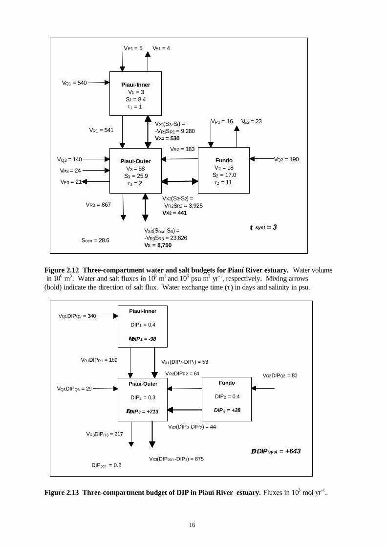
Salt and water budgetsThe smaller volume and higher freshwater discharge produce a very low water exchange time (about aday) to the inner Piauí River estuary (Figure 2.12). The Piauí River outer estuary exhibits a similarwater exchange times (about 2 days). The Fundo River, with less than a half the volume of the former,has a higher exchange time (11 days). Tidal mixing is the main process responsible for water renewalin the three compartments. In the Piauí and Fundo rivers this effect is striking.

Budgets of nonconservative materialsDIP balanceThe subdivision of these estuarine sections reveals that net heterotrophy is restricted to the outer Piauíestuary (Figure 2.13; ∆DIP = +713x103 mol yr-1; +23 mmol m-2 yr-1) and the Fundo River (+28x103

mol yr-1; +3 mmol m-2 yr-1). The inner Piauí estuary shows negative ∆DIP (-98x103 mol yr-1, or -33mmol m-2 yr-1). Adding up these compartments, the 3-compartment model yields ∆DIP for the wholesystem of +643x103 mol yr-1 (+15 mmol m-2 yr-1), compared to the 1-box model results of +184x103

mol yr-1. It is assumed that the 3-box model is the more accurate resolution of ∆DIP.

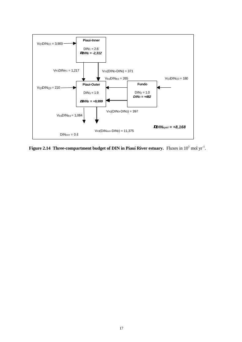
DIN balance∆DIN balance exhibited the same pattern as ∆DIP (Figure 2.14). ∆DIN in the outer Piauí estuary was+9,999x103 mol yr-1 (+323 mmol m-2 yr-1), and Fundo was +482x103mol yr-1 (48 mmol m-2 yr-1). InnerPiauí estuary showed a negative ∆DIN flux of -2,312x103 mol yr-1 (-771 mmol m-2 yr-1). The 3-boxmodel thus yields a whole-system ∆DIN of +8.2x106 mol yr-1 (+187 mmol m-2 yr-1). Again, theseresults are substantially higher than the results from the 1-box model (+2.2x106 mol yr-1).

Stoichiometric calculations based on the 3-box modelIn the stoichiometric calculations (Table 2.2), we present (p-r) estimated using both the Redfield C:Pratio and that of average suspended organic matter in each box. There is about a 4-fold difference inestimated net metabolism for the whole system, depending on the choice of C:P, but in either case thesystem is net heterotrophic (p-r <0). The polluted portion of the estuary (inner Piauí River) is stronglyautotrophic but accounts for less than 10% of the estuary area. Rio Fundo is a minor contributor to thesystem metabolism, and the outer Piauí River dominates the net metabolism. Whichever ratio is used,estimated net metabolic rates for the system are much higher than those obtained by the 1-boxapproach.

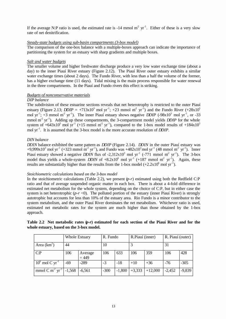
Table 2.2 Net metabolic rates (p-r) estimated for each section of the Piauí River and for thewhole estuary, based on the 3-box model.

Whole Estuary R. Fundo R.Piauí (inner) R. Piauí (outer)

Area (km2) 44 10 3 31

C:P 106 Average= 449

106 633 106 359 106 428

106 mol C yr-1 -69 -289 -3 -18 +10 +36 -76 -305

mmol C m-2 yr-1 -1,568 -6,561 -300 -1,800 +3,333 +12,000 -2,452 -9,839

14

Table 2.3 summarizes estimates of (nfix-denit). The system overall is a very slight net denitrifyingsystem. The calculated rate with the 3-box model is higher than the calculations based on the 1-boxmodel; in both cases the net rate for the whole system is low.

Table 2.3 Net nitrogen fixation - denitrification (nfix-denit) estimated for each section of thePiauí River and for the whole estuary, based on the 3-box model.

Whole Estuary R. Fundo R. Piauí (inner) R. Piauí (outer)

Area (km2) 44 10 3 31

N:P 16 Average= 19

16 19 16 18 16 19

103 mol N yr-1 -2,120 -4,048 +34 -50 -744 -548 -1,409 -3,548

mmol N m-2 yr-1 -48 -92 +3 -5 -248 -183 -45 -114

ConclusionsApparently the Rio Piauí estuary is a net heterotrophic system, denitrifying at a very slow rate. Theexact results obtained are very sensitive to both the C:P and the N:P ratios of the reacting material,although the qualitative results are the same in either case.

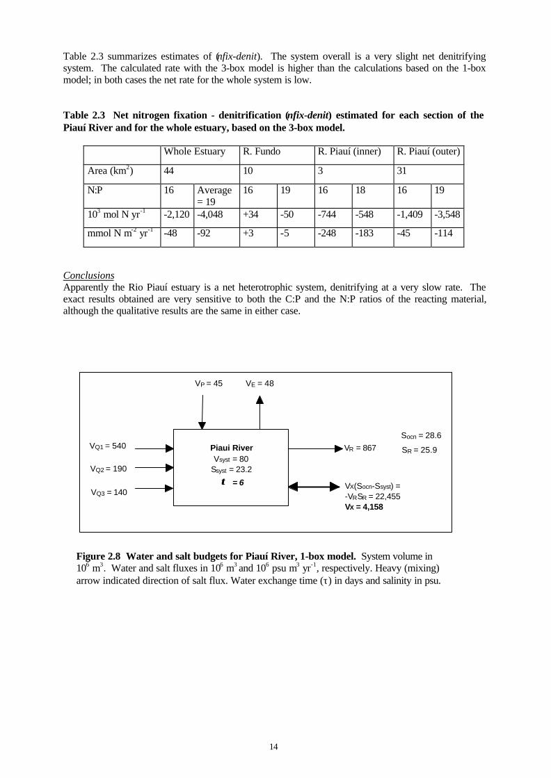
Figure 2.8 Water and salt budgets for Piauí River, 1-box model. System volume in106 m3. Water and salt fluxes in 106 m3 and 106 psu m3 yr-1, respectively. Heavy (mixing)arrow indicated direction of salt flux. Water exchange time (τ) in days and salinity in psu.

Piaui River Vsyst = 80

Ssyst = 23.2

τ τ = 6

VP = 45 VE = 48

VQ1 = 540

VQ2 = 190

VQ3 = 140

VR = 867

Socn = 28.6

SR = 25.9

VX(Socn-Ssyst) = -VRSR = 22,455 VX = 4,158

15

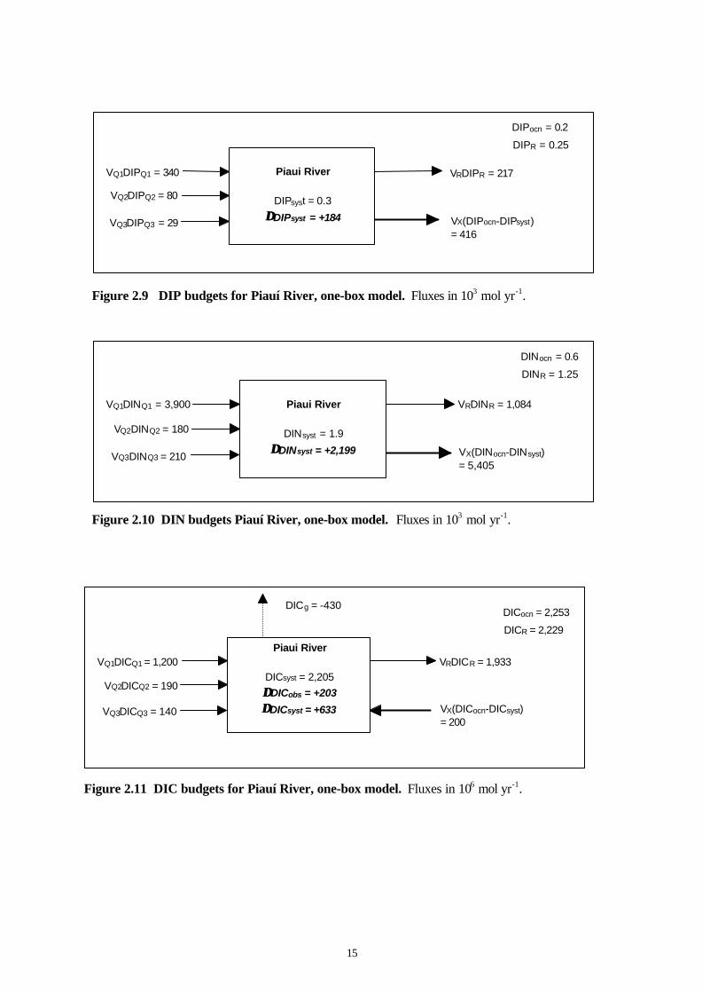
Figure 2.9 DIP budgets for Piauí River, one-box model. Fluxes in 103 mol yr-1.

Figure 2.10 DIN budgets Piauí River, one-box model. Fluxes in 103 mol yr-1.

Figure 2.11 DIC budgets for Piauí River, one-box model. Fluxes in 106 mol yr-1.

Piaui River

DIPsyst = 0.3

∆∆DIPsyst = +184

VQ1DIPQ1 = 340

VQ2DIPQ2 = 80

VQ3DIPQ3 = 29

VRDIPR = 217

DIPocn = 0.2

DIPR = 0.25

VX(DIPocn-DIPsyst) = 416

Piaui River

DINsyst = 1.9

∆∆DINsyst = +2,199

VQ1DINQ1 = 3,900

VQ2DINQ2 = 180

VQ3DINQ3 = 210

VRDINR = 1,084

DINocn = 0.6

DINR = 1.25

VX(DINocn-DINsyst) = 5,405

Piaui River

DICsyst = 2,205

∆∆DICobs = +203 ∆∆DICsyst = +633

VQ1DICQ1 = 1,200

VQ2DICQ2 = 190

VQ3DICQ3 = 140

VRDICR = 1,933

DICocn = 2,253

DICR = 2,229

VX(DICocn-DICsyst) = 200

DICg = -430

16

Figure 2.12 Three-compartment water and salt budgets for Piauí River estuary. Water volume in 106 m3. Water and salt fluxes in 106 m3 and 106 psu m3 yr-1, respectively. Mixing arrows(bold) indicate the direction of salt flux. Water exchange time (τ) in days and salinity in psu.

Figure 2.13 Three-compartment budget of DIP in Piauí River estuary. Fluxes in 103 mol yr-1.

Piaui-Inner V1 = 3

S1 = 8.4 τ1 = 1

Fundo V2 = 18

S2 = 17.0 τ2 = 11

Piaui-Outer V3 = 58

S3 = 25.9 τ3 = 2

VQ1 = 540

VX1(S3-St) = -VR1SR1 = 9,280 VX1 = 530

VP1 = 5 VE1 = 4

VQ3 = 140

VR1 = 541

VP2 = 16 VE2 = 23

VX2(S3-S2) = -VR2SR2 = 3,925 VX2 = 441

VX3(Socn-S3) = -VR3SR3 = 23,626 VX = 8,750

VQ2 = 190

VR3 = 867

VR2 = 183

Socn = 28.6

VP3 = 24

VE3 = 21

ττ syst = 3

Piaui-Inner

DIP1 = 0.4

∆∆DIP1 = -98

Fundo

DIP2 = 0.4

DIP3 = +28

Piaui-Outer

DIP3 = 0.3

∆∆DIP3 = +713

VQ1DIPQ1 = 340

VX1(DIP3-DIPt) = 53

VQ3DIPQ3 = 29

VR1DIPR1 = 189

VX2(DIP3-DIP2) = 44

VX3(DIPocn -DIP3) = 875

VQ2DIPQ2 = 80

VR3DIPR3 = 217

VR2DIPR2 = 64

DIPocn = 0.2

∆ ∆ DIPsyst = +643

17

Figure 2.14 Three-compartment budget of DIN in Piauí River estuary. Fluxes in 103 mol yr-1.

Piaui-Inner

DIN1 = 2.6 ∆∆DIN1 = -2,312

Fundo

DIN2 = 1.0 DIN3 = +482

Piaui-Outer

DIN3 = 1.9

∆∆DIN3 = +9,999

VQ1DINQ1 = 3,900

VX1(DIN3-DINt) = 371

VQ3DINQ3 = 210

VR1DINR1 = 1,217

VX2(DIN3-DIN2) = 397

VX3(DINocn-DIN3) = 11,375

VQ2DINQ2 = 180

VR3DINR3 = 1,084

VR2DINR2 = 265

DINocn = 0.6

∆∆DINsyst = +8,168

18

2.3 Maricá-Guarapina coastal lagoons, Rio de Janeiro State

Erminda da C.G. Couto, Nicole A.C. Zyngier, Viviane R. Gomes , Bastiaan A. Knoppers andMarcelo F. Landim de Souza

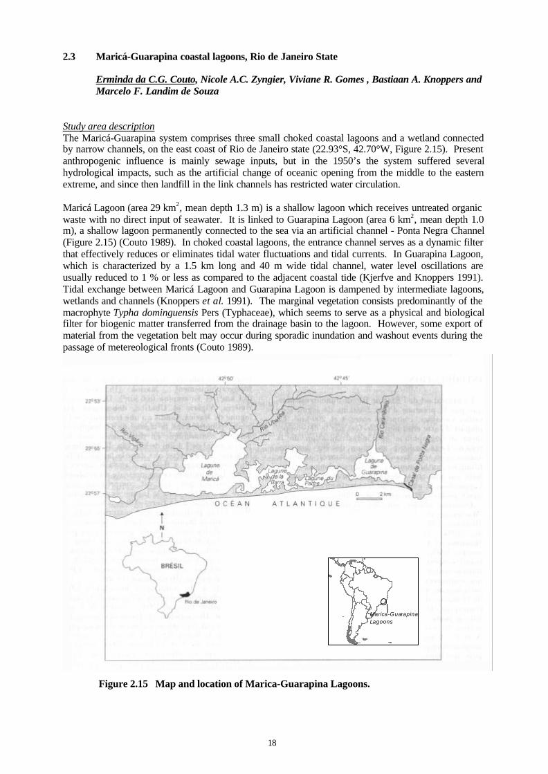
Study area descriptionThe Maricá-Guarapina system comprises three small choked coastal lagoons and a wetland connectedby narrow channels, on the east coast of Rio de Janeiro state (22.93°S, 42.70°W, Figure 2.15). Presentanthropogenic influence is mainly sewage inputs, but in the 1950’s the system suffered severalhydrological impacts, such as the artificial change of oceanic opening from the middle to the easternextreme, and since then landfill in the link channels has restricted water circulation.

Maricá Lagoon (area 29 km2, mean depth 1.3 m) is a shallow lagoon which receives untreated organicwaste with no direct input of seawater. It is linked to Guarapina Lagoon (area 6 km2, mean depth 1.0m), a shallow lagoon permanently connected to the sea via an artificial channel - Ponta Negra Channel(Figure 2.15) (Couto 1989). In choked coastal lagoons, the entrance channel serves as a dynamic filterthat effectively reduces or eliminates tidal water fluctuations and tidal currents. In Guarapina Lagoon,which is characterized by a 1.5 km long and 40 m wide tidal channel, water level oscillations areusually reduced to 1 % or less as compared to the adjacent coastal tide (Kjerfve and Knoppers 1991).Tidal exchange between Maricá Lagoon and Guarapina Lagoon is dampened by intermediate lagoons,wetlands and channels (Knoppers et al. 1991). The marginal vegetation consists predominantly of themacrophyte Typha dominguensis Pers (Typhaceae), which seems to serve as a physical and biologicalfilter for biogenic matter transferred from the drainage basin to the lagoon. However, some export ofmaterial from the vegetation belt may occur during sporadic inundation and washout events during thepassage of metereological fronts (Couto 1989).

Marica-Guarapina Lagoons

Figure 2.15 Map and location of Marica-Guarapina Lagoons.

19

This system exhibits pronounced annual cycles of salinity (Moreira 1988; Couto 1989; Machado1989). Salinity changes are always smallest in the internal cells of lagoon systems. However, intenserain events may induce drastic salinity changes. These events result in marked biogeochemical andecological responses (Knoppers and Moreira 1988).

Primary production is dominated by phytoplankton production. In the summer Guarapina Lagoon isdominated by planktonic cyanobacteria (Moreira 1988). Mean annual primary production range is~300-400 g C m-2 yr-1 in Guarapina lagoon (Machado and Knoppers 1988; Moreira 1989). The highestfraction of suspended detrital organic matter is encountered during the less productive period duringlate autumn and winter. Most of the suspended detritus originates from autotrophic production, asindicated by the relatively low particulate organic carbon to nitrogen ratios, with C:N by weight lessthan 9:1, and seems to be an important source of nutrients for primary production in the spring(Moreira 1988; Knoppers and Moreira, 1990; Moreira and Knoppers 1990). The presence of largesuspended detrital pools has been confirmed for Barra Lagoon (Carmouze et al. 1993) and GuarapinaLagoon (Moreira 1988).

Measurements of nutrient release rates from the sediment-water interface have been made in Maricá(Fernex et al. 1992), Barra (Kuroshima 1995) and Guarapina (Machado 1989) lagoons. The resultsreflect seasonal variability of benthic nutrient fluxes, with the highest flux usually occurring during thesummer when primary production is highest.

The system presented marked seasonal shifts between autotrophy and heterotrophy, with autotrophydominating during the summer and heterotrophy during the winter. Net autotrophy and heterotrophyare equal on an annual basis (Knoppers and Kjerfve, in press.). In Maricá and Barra Lagoons sporadicdystrophic crises and fish kills induce nutrient pulses (Esteves 1992; Carmouze et al. 1993).

A consistent data set for Maricá Lagoon does not exist. Knoppers et al. (1991) presented concentrationranges from sporadic sampling effort conducted by FEEMA. Nutrient and chlorophyll aconcentrations and the ratio of total inorganic nitrogen to total inorganic phosphorus (TIN/TIP) are farless in Guarapina Lagoon than in the other lagoons along the Rio de Janeiro coast (Knoppers et al.1991). The major fraction of organic matter is stored in phytoplankton. Ammonia was the majorcomponent (>50%) of TIN with major sources being the bottom in Guarapina (Machado 1989) andhuman effluents in Maricá. An estimate based on the per capita load of phosphorus from thepopulation in Maricá City (38,500) suggests that this lagoon receives large amounts of effluentdischarges (FEEMA 1987). The N/P ratio indicated a trend towards nitrogen limitation. Loading fromthe Guarapina drainage basin is minimal and conditions closely resemble a natural state (Figueiredo etal. 1996). However, Guarapina Lagoon receives a considerable load from its adjacent interior lagoons(Padre, Barra and Maricá lagoons). The source of the high TIN load (ammonia) in Guarapina isprimarily due to decomposition of benthic macroalgae (Cladophora vagabunda) in Padre Lagoon. Theintermediate lagoons change their role in the transfer of matter and nutrients seasonally betweenMaricá and Guarapina lagoons, alternately functioning as a filter and as an internal recycling source ofreleasing nutrients (Knoppers et al. 1991). Using both total phosphorus and chlorophyll aconcentrations as trophic state (TP) indices demonstrates that Maricá, Barra, Padre and Guarapinalagoons presented an eutrophic state.

Available early data was compiled to construct a preliminary nutrient budget and apply the LOICZbiogeochemical approach (Gordon et al. 1996) on an annual basis.

Water and salt balanceTotal water residence time was about 314 days in Maricá, 25 days in Guarapina, and only 185 daysconsidering the whole system. The annual average salinity was higher in Guarapina (17 psu) thanMaricá (5 psu). In Guarapina Lagoon mixing with the adjacent sea is continuous. Tidal exchangebetween Maricá and Guarapina lagoons is dampened by the narrow channel. In this lagoon a smallresidual flow is produced by hydraulic gradient. This results in a high residence time.

20

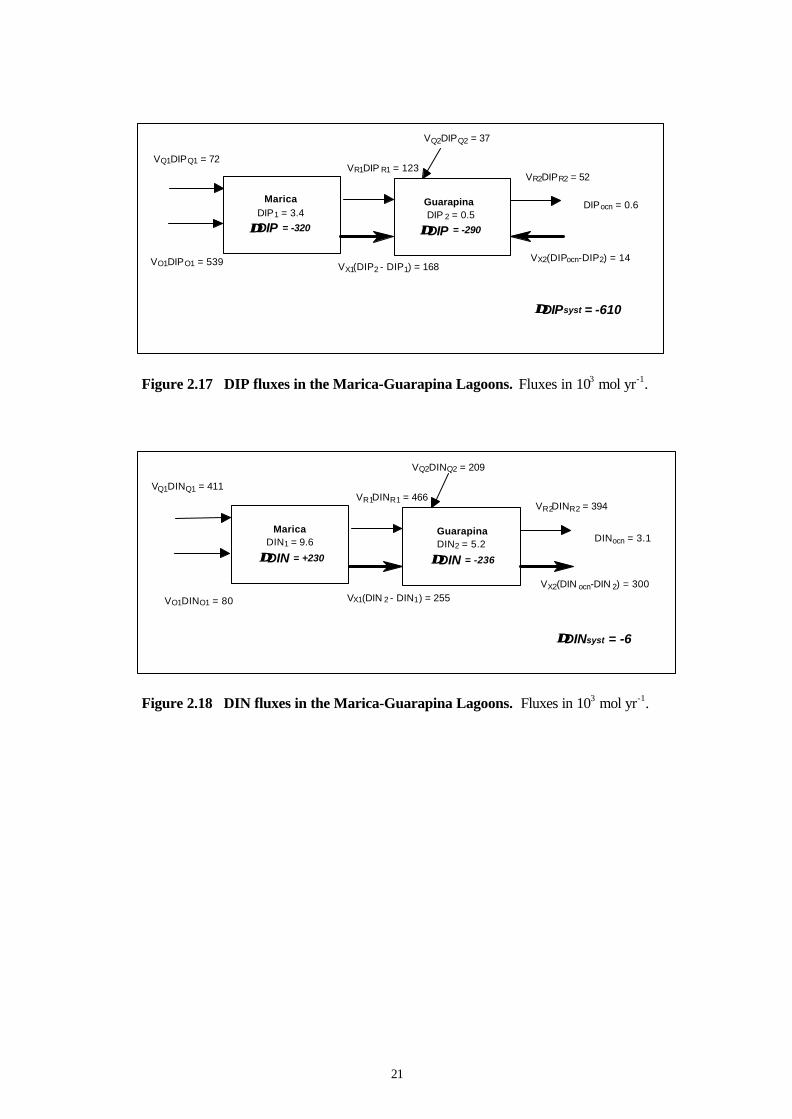
Nonconservative materials balanceDissolved inorganic phosphorus and nitrogen concentrations were higher in Maricá (3.4 µM DIP and9.6 µM DIN) than Guarapina (0.5 µM DIP and 5.2 µM DIN). Most of the hydraulic flux DIP exportedfrom Maricá (90.4%) is retained in Guarapina. This resulted in net seaward fluxes of 3x103 moles DIPyr-1.

The negative net nonconservative fluxes of DIP and DIN show that autotrophic processes prevail in thesystem. A small fraction of DIN (3.7 %) exported from Maricá is retained in Guarapina. This resultedin net seaward fluxes of 694x103 moles DIN yr-1.

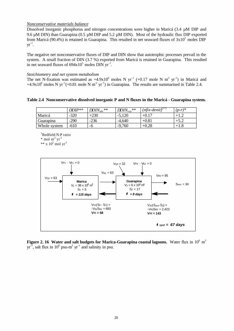
Stoichiometry and net system metabolismThe net N-fixation was estimated as +4.9x106 moles N yr-1 (+0.17 mole N m-2 yr-1) in Maricá and+4.9x106 moles N yr-1(+0.81 mole N m-2 yr-1) in Guarapina. The results are summarised in Table 2.4.

Table 2.4 Nonconservative dissolved inorganic P and N fluxes in the Maricá - Guarapina system.

∆DIP** ∆DINobs** ∆DINexp** (nfix-denit)(1*) (p-r)*Maricá -320 +230 -5,120 +0.17 +1.2Guarapina -290 -236 -4,640 +0.81 +5.2Whole system -610 -6 -9,760 +0.28 +1.8

1Redfield N:P ratio* mol m-2 yr-1

** x 103 mol yr-1

Figure 2. 16 Water and salt budgets for Marica-Guarapina coastal lagoons. Water flux in 106 m3

yr-1, salt flux in 106 psu-m3 yr-1 and salinity in psu.

VP1 - VE1 = 0

VQ1 = 63VR2 = 95

Socn = 34

VX2(Socn-S2) = -VR2SR2 = 2,423 VX2 = 143

VX1(S2 - S1) = -VR1SR1 = 693 VX1 = 58

VP2 - VE2 = 0

VR1 = 63

VQ2 = 32

τ τ syst = 67 days

Marica V1 = 38 x 10 m

S1 = 5

τ τ = 115 days

6 3Guarapina

V2 = 6 x 10 m S2 = 17

τ τ = 8 days

6 3

21

Figure 2.17 DIP fluxes in the Marica-Guarapina Lagoons. Fluxes in 103 mol yr-1.

Figure 2.18 DIN fluxes in the Marica-Guarapina Lagoons. Fluxes in 103 mol yr-1.

Guarapina DIP 2 = 0.5

∆∆DIP = -290

VQ1DIPQ1 = 72

VR2DIPR2 = 52

DIPocn = 0.6

VX2(DIPocn-DIP2) = 14

Marica DIP1 = 3.4

∆∆DIP = -320

VX1(DIP2 - DIP1) = 168

VR1DIP R1 = 123

VQ2DIPQ2 = 37

VO1DIPO1 = 539

∆∆DIPsyst = -610

Guarapina DIN2 = 5.2

∆∆DIN = -236

VQ1DINQ1 = 411

VR2DINR2 = 394

DINocn = 3.1

VX2(DIN ocn-DIN 2) = 300

Marica DIN1 = 9.6

∆ ∆DIN = +230

VX1(DIN 2 - DIN1) = 255

VR1DINR1 = 466

VQ2DINQ2 = 209

VO1DINO1 = 80

∆∆DINsyst = -6

22

2.4 Piratininga-Itaipú Coastal Lagoons, Rio de Janeiro State

Erminda C.G. Couto, Nicole A.C. Zyngier and M.F.Landim de Souza

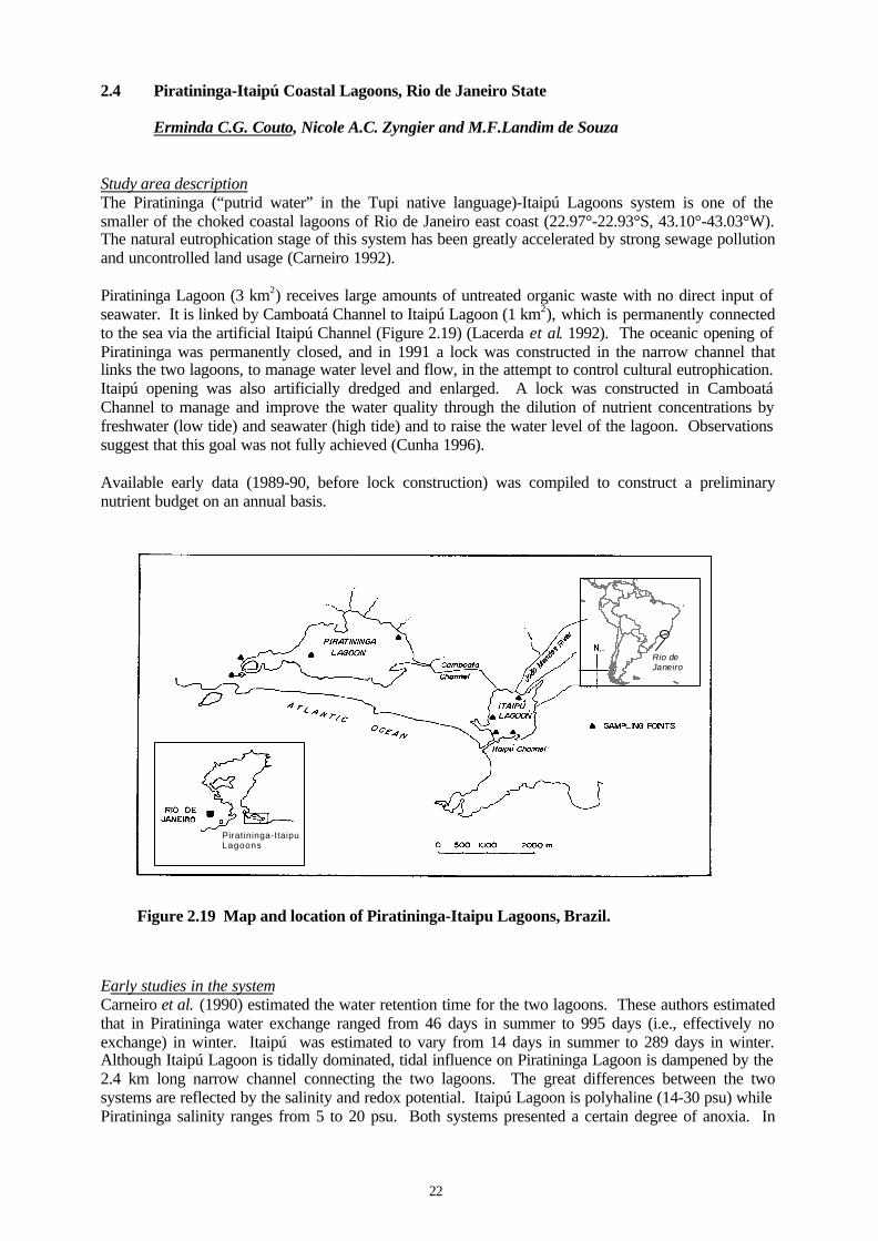
Study area descriptionThe Piratininga (“putrid water” in the Tupi native language)-Itaipú Lagoons system is one of thesmaller of the choked coastal lagoons of Rio de Janeiro east coast (22.97°-22.93°S, 43.10°-43.03°W).The natural eutrophication stage of this system has been greatly accelerated by strong sewage pollutionand uncontrolled land usage (Carneiro 1992).

Piratininga Lagoon (3 km2) receives large amounts of untreated organic waste with no direct input ofseawater. It is linked by Camboatá Channel to Itaipú Lagoon (1 km2), which is permanently connectedto the sea via the artificial Itaipú Channel (Figure 2.19) (Lacerda et al. 1992). The oceanic opening ofPiratininga was permanently closed, and in 1991 a lock was constructed in the narrow channel thatlinks the two lagoons, to manage water level and flow, in the attempt to control cultural eutrophication.Itaipú opening was also artificially dredged and enlarged. A lock was constructed in CamboatáChannel to manage and improve the water quality through the dilution of nutrient concentrations byfreshwater (low tide) and seawater (high tide) and to raise the water level of the lagoon. Observationssuggest that this goal was not fully achieved (Cunha 1996).

Available early data (1989-90, before lock construction) was compiled to construct a preliminarynutrient budget on an annual basis.

Early studies in the systemCarneiro et al. (1990) estimated the water retention time for the two lagoons. These authors estimatedthat in Piratininga water exchange ranged from 46 days in summer to 995 days (i.e., effectively noexchange) in winter. Itaipú was estimated to vary from 14 days in summer to 289 days in winter.Although Itaipú Lagoon is tidally dominated, tidal influence on Piratininga Lagoon is dampened by the2.4 km long narrow channel connecting the two lagoons. The great differences between the twosystems are reflected by the salinity and redox potential. Itaipú Lagoon is polyhaline (14-30 psu) whilePiratininga salinity ranges from 5 to 20 psu. Both systems presented a certain degree of anoxia. In

Rio deJaneiro

Piratininga-ItaipuLagoons

Figure 2.19 Map and location of Piratininga-Itaipu Lagoons, Brazil.

23

Piratininga anoxia extends throughout the water column and attains very low Eh values (-302 to +130mV), whereas in Itaipú, anoxia is restricted to bottom waters (-66 to +20 mV), as surface waters arewell oxidized (+210 to +236 mV). In general, bottom waters in both systems were relatively more acidand warm (Lacerda et al. 1992). Sporadic dystrophic crises and fish kills induce nutrients pulses(Carmouze et al. 1993).

Piratininga Lagoon is dominated by the benthic macroalga Chara hornemanii Wallm. Cladophoravagabunda is also present. In 1990 C. hornemanii occupied aproximately 60% of the lagoon area andrepresented a considerable standing stock of organic matter (53g C m-2, 10g N m-2, and 0.6g P m-2).During their growth period (winter through summer), the macroalgae assimilate nutrients from thewater column. During the autumn decay period, nutrients are released to the water. Phytoplanktonstanding crop appears to be negligible. High chlorophyll a concentrations were only measured neardecaying populations of C. hornemanii.

Nutrient and chlorophyll a concentrations and the ratio of total inorganic nitrogen to total inorganicphosphorus (DIN/DIP) are far greater in Piratininga Lagoon than in the other lagoons along the Rio deJaneiro coast (Knoppers et al. 1991). The major fraction of organic matter in Piratininga is stored inseaweed. In Itaipú organic matter is present in phytoplankton. Ammonium was the major component(>50%) of DIN, with major sources in Piratininga being human effluents and algal banks. The use oftrophic state indices as total phosphorus (TP) and chlorophyll a concentrations demonstrate that ItaipúLagoon is in the upper limit of mesotrophic state, with the TP level indicating an eutrophic state,whereas chlorophyll a indicates a mesotrophic state. This may be attributed to the high TP load fromPiratininga Lagoon and the high DIP remineralized in sediments, released by frequent resuspension ofbottom materials by strong tidal currents. Piratininga Lagoon is permanently hypertrophic. In shallowwaters, continuous effluent loading, and long water exchange time allow the growth of extensive algalbanks. Although nutrient loading into Itaipú Lagoon is higher than for Piratininga Lagoon, fast tidaldilution mitigates the effects of the high effluent loading (Knoppers et al. 1991).

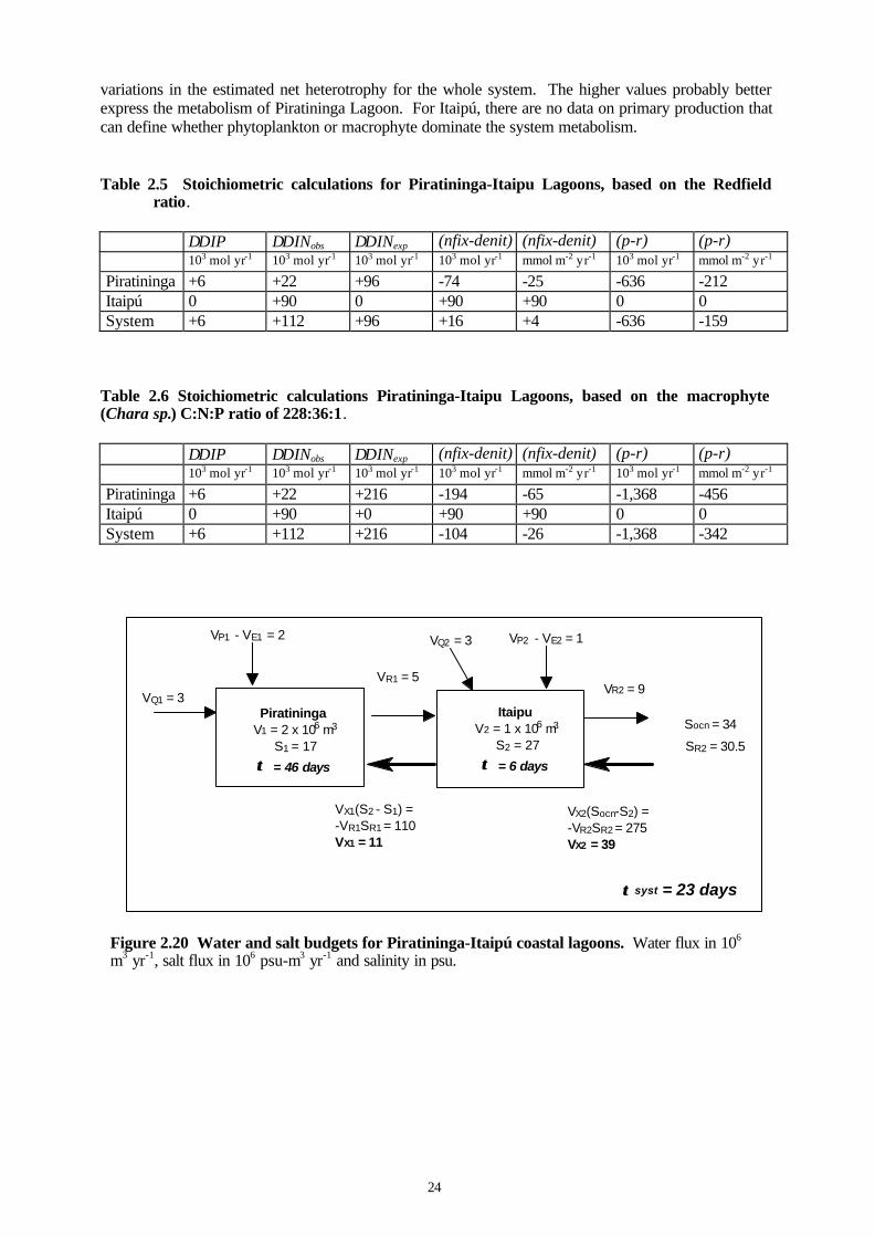
Salt and water balanceTotal water exchange times calculated from the water and salt budgets (Figure 2.20) ranged from 46days in Piratininga to about 6 days in Itaipú. These values compare with the much longer estimates inthe literature (Knoppers et al. 1991). Mixing exchange seems to be the main water renewal process toboth lagoons, despite the long and narrow channel linking them.

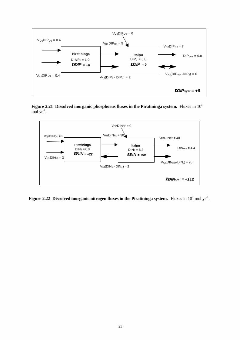
Nonconservative materials balanceDIP balanceThe average concentrations of DIP are almost equal in both lagoons (Figure 2.21). The resulting fluxcalculations demonstrate that the lagoons are sources of nutrients and are interpreted to indicate thatheterotrophic processes prevail. It should be kept in mind that the episodic anoxia in the water columnof some areas favour the release of DIP, and to an uncertain degree overestimate the heterotrophy.Both lagoons are DIP sources to coastal waters.

DIN balanceThe difference of DIN concentrations between the lagoons was small, as for DIP (Figure 2.22).Nonconservative fluxes were positive, being higher in the smaller Itaipú Lagoon. The whole system isa source of DIN delivery to coastal waters.

Stoichiometric calculationsThe net N fixation-denitrification rates (nfix-denit) were low in both systems, using Redfield or themacrophyte (C. hornemanii) C:N:P ratio of about 228:36:1 (Tables 2.5, 2.6). Piratininga exhibitedslight net denitrification, while Itaipu apparently fixed a small amount of N. The whole systemapparently ranged from very slight net N-fixation to net denitrification, depending on the choice ofRedfield or C. hornemanii N:P ratios.

There is higher net heterotrophy in Piratininga Lagoon, with the estimated rate being dependent on theC:P ratio used. The utilization of these different ratios for organic matter can produce a factor of two

24

variations in the estimated net heterotrophy for the whole system. The higher values probably betterexpress the metabolism of Piratininga Lagoon. For Itaipú, there are no data on primary production thatcan define whether phytoplankton or macrophyte dominate the system metabolism.

Table 2.5 Stoichiometric calculations for Piratininga-Itaipu Lagoons, based on the Redfieldratio.

∆DIP ∆DINobs ∆DINexp (nfix-denit) (nfix-denit) (p-r) (p-r)103 mol yr-1 103 mol yr-1 103 mol yr-1 103 mol yr-1 mmol m-2 yr-1 103 mol yr-1 mmol m-2 yr-1

Piratininga +6 +22 +96 -74 -25 -636 -212Itaipú 0 +90 0 +90 +90 0 0System +6 +112 +96 +16 +4 -636 -159

Table 2.6 Stoichiometric calculations Piratininga-Itaipu Lagoons, based on the macrophyte(Chara sp.) C:N:P ratio of 228:36:1.

∆DIP ∆DINobs ∆DINexp (nfix-denit) (nfix-denit) (p-r) (p-r)103 mol yr-1 103 mol yr-1 103 mol yr-1 103 mol yr-1 mmol m-2 yr-1 103 mol yr-1 mmol m-2 yr-1

Piratininga +6 +22 +216 -194 -65 -1,368 -456Itaipú 0 +90 +0 +90 +90 0 0System +6 +112 +216 -104 -26 -1,368 -342

Figure 2.20 Water and salt budgets for Piratininga-Itaipú coastal lagoons. Water flux in 106

m3 yr-1, salt flux in 106 psu-m3 yr-1 and salinity in psu.

VP1 - VE1 = 2

VQ1 = 3VR2 = 9

Socn = 34

SR2 = 30.5

VX2(Socn-S2) = -VR2SR2 = 275 VX2 = 39

VX1(S2 - S1) = -VR1SR1 = 110 VX1 = 11

VP2 - VE2 = 1

VR1 = 5

VQ2 = 3

τ τ syst = 23 days

Piratininga V1 = 2 x 10 m

S1 = 17

τ τ = 46 days

6 3Itaipu

V2 = 1 x 10 m S2 = 27

τ τ = 6 days

6 3

25

Figure 2.21 Dissolved inorganic phosphorus fluxes in the Piratininga system. Fluxes in 103

mol yr-1.

Figure 2.22 Dissolved inorganic nitrogen fluxes in the Piratininga system. Fluxes in 103 mol yr-1.

Itaipu DIP2 = 0.8

∆∆DIP = 0

VQ1DIPQ1 = 0.4

VR2DIPR2 = 7

DIPocn = 0.8

VX2(DIPocn-DIP2) = 0

Piratininga

DINP1 = 1.0 ∆∆DIP = +6

VX1(DIP2 - DIP1) = 2

VR1DIPR1 = 5

VQ2DIPQ2 = 0

VO1DIPO1 = 0.4

∆∆DIPsyst = +6

Itaipu DIN2 = 6.2 ∆∆DIN = +90

VQ1DINQ1 = 3 VR2DINR2 = 48

DINocn = 4.4

VX2(DINocn-DIN2) = 70

Piratininga DIN1 = 6.0

∆ ∆DIN = +22

VX1(DIN2 - DIN1) = 2

VR1DINR1 = 30

VQ2DINQ2 = 0

VO1DINO1 = 3

∆∆DINsyst = +112

26

2.5 Paranaguá Bay estuarine complex, Paraná State

E. Marone, Eunice C. Machado, R.M. Lopes and E.T. Silva

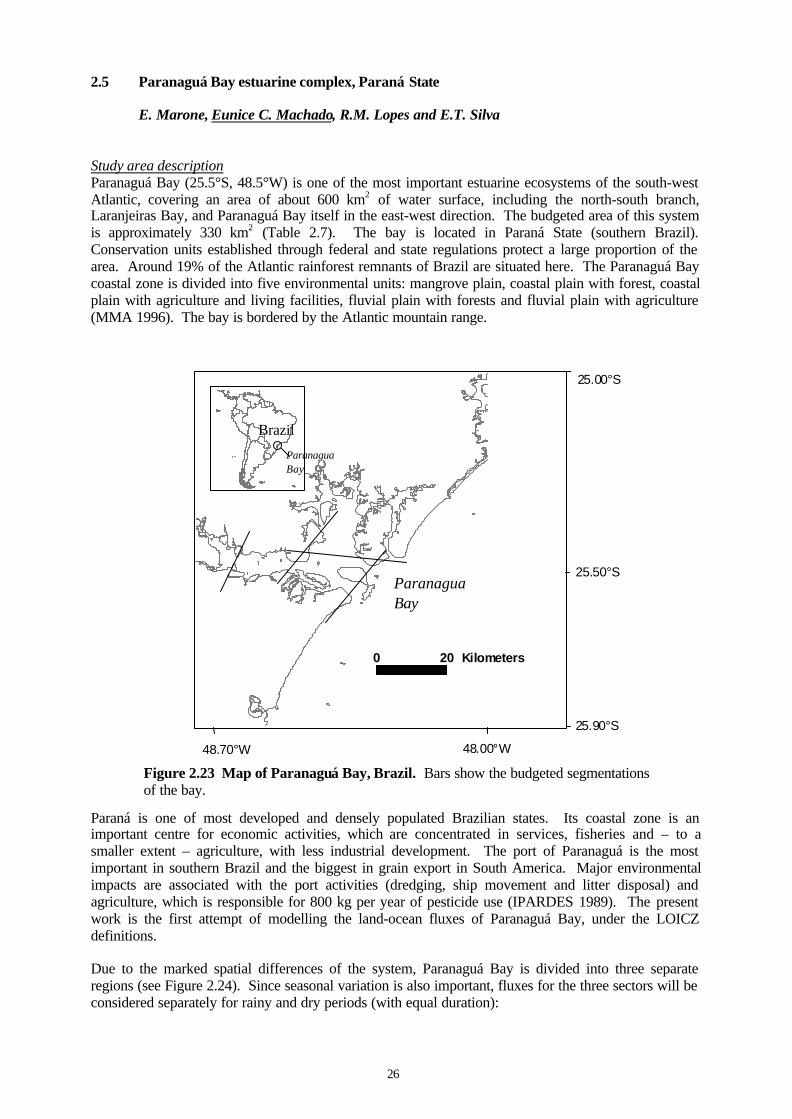
Study area descriptionParanaguá Bay (25.5°S, 48.5°W) is one of the most important estuarine ecosystems of the south-westAtlantic, covering an area of about 600 km2 of water surface, including the north-south branch,Laranjeiras Bay, and Paranaguá Bay itself in the east-west direction. The budgeted area of this systemis approximately 330 km2 (Table 2.7). The bay is located in Paraná State (southern Brazil).Conservation units established through federal and state regulations protect a large proportion of thearea. Around 19% of the Atlantic rainforest remnants of Brazil are situated here. The Paranaguá Baycoastal zone is divided into five environmental units: mangrove plain, coastal plain with forest, coastalplain with agriculture and living facilities, fluvial plain with forests and fluvial plain with agriculture(MMA 1996). The bay is bordered by the Atlantic mountain range.

25.90°S

25.50°S

25.00°S

48.70°W 48.00°W

0 20 Kilometers

Paraná is one of most developed and densely populated Brazilian states. Its coastal zone is animportant centre for economic activities, which are concentrated in services, fisheries and – to asmaller extent – agriculture, with less industrial development. The port of Paranaguá is the mostimportant in southern Brazil and the biggest in grain export in South America. Major environmentalimpacts are associated with the port activities (dredging, ship movement and litter disposal) andagriculture, which is responsible for 800 kg per year of pesticide use (IPARDES 1989). The presentwork is the first attempt of modelling the land-ocean fluxes of Paranaguá Bay, under the LOICZdefinitions.

Due to the marked spatial differences of the system, Paranaguá Bay is divided into three separateregions (see Figure 2.24). Since seasonal variation is also important, fluxes for the three sectors will beconsidered separately for rainy and dry periods (with equal duration):

Brazil

ParanaguaBay

Figure 2.23 Map of Paranaguá Bay, Brazil. Bars show the budgeted segmentationsof the bay.

ParanaguaBay

27

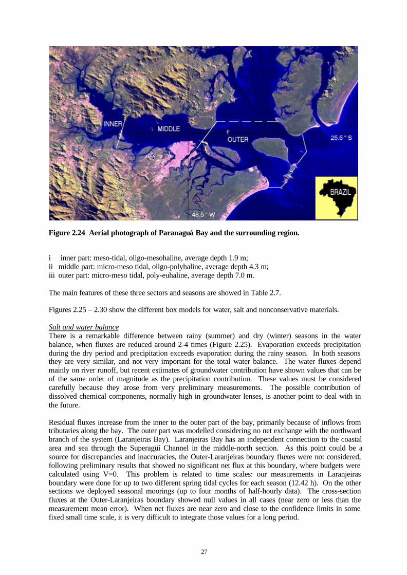
Figure 2.24 Aerial photograph of Paranaguá Bay and the surrounding region.

i inner part: meso-tidal, oligo-mesohaline, average depth 1.9 m;ii middle part: micro-meso tidal, oligo-polyhaline, average depth 4.3 m;iii outer part: micro-meso tidal, poly-euhaline, average depth 7.0 m.

The main features of these three sectors and seasons are showed in Table 2.7.

Figures 2.25 – 2.30 show the different box models for water, salt and nonconservative materials.

Salt and water balanceThere is a remarkable difference between rainy (summer) and dry (winter) seasons in the waterbalance, when fluxes are reduced around 2-4 times (Figure 2.25). Evaporation exceeds precipitationduring the dry period and precipitation exceeds evaporation during the rainy season. In both seasonsthey are very similar, and not very important for the total water balance. The water fluxes dependmainly on river runoff, but recent estimates of groundwater contribution have shown values that can beof the same order of magnitude as the precipitation contribution. These values must be consideredcarefully because they arose from very preliminary measurements. The possible contribution ofdissolved chemical components, normally high in groundwater lenses, is another point to deal with inthe future.

Residual fluxes increase from the inner to the outer part of the bay, primarily because of inflows fromtributaries along the bay. The outer part was modelled considering no net exchange with the northwardbranch of the system (Laranjeiras Bay). Laranjeiras Bay has an independent connection to the coastalarea and sea through the Superagüí Channel in the middle-north section. As this point could be asource for discrepancies and inaccuracies, the Outer-Laranjeiras boundary fluxes were not considered,following preliminary results that showed no significant net flux at this boundary, where budgets werecalculated using V=0. This problem is related to time scales: our measurements in Laranjeirasboundary were done for up to two different spring tidal cycles for each season (12.42 h). On the othersections we deployed seasonal moorings (up to four months of half-hourly data). The cross-sectionfluxes at the Outer-Laranjeiras boundary showed null values in all cases (near zero or less than themeasurement mean error). When net fluxes are near zero and close to the confidence limits in somefixed small time scale, it is very difficult to integrate those values for a long period.

28

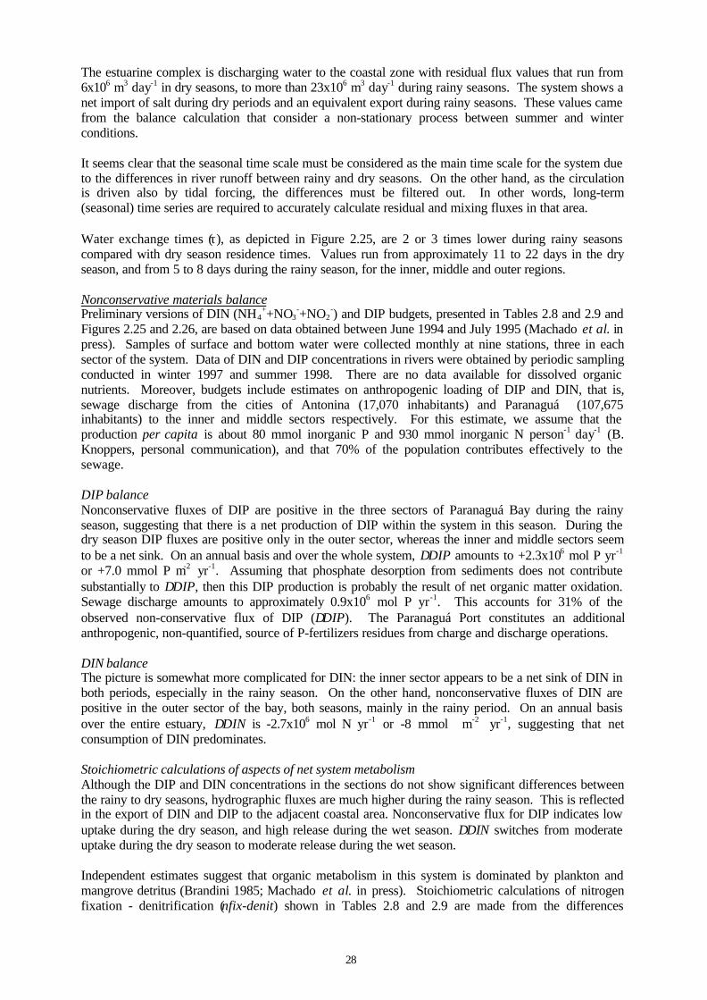
The estuarine complex is discharging water to the coastal zone with residual flux values that run from6x106 m3 day-1 in dry seasons, to more than 23x106 m3 day-1 during rainy seasons. The system shows anet import of salt during dry periods and an equivalent export during rainy seasons. These values camefrom the balance calculation that consider a non-stationary process between summer and winterconditions.

It seems clear that the seasonal time scale must be considered as the main time scale for the system dueto the differences in river runoff between rainy and dry seasons. On the other hand, as the circulationis driven also by tidal forcing, the differences must be filtered out. In other words, long-term(seasonal) time series are required to accurately calculate residual and mixing fluxes in that area.

Water exchange times (τ), as depicted in Figure 2.25, are 2 or 3 times lower during rainy seasonscompared with dry season residence times. Values run from approximately 11 to 22 days in the dryseason, and from 5 to 8 days during the rainy season, for the inner, middle and outer regions.

Nonconservative materials balancePreliminary versions of DIN (NH4

++NO3-+NO2

-) and DIP budgets, presented in Tables 2.8 and 2.9 andFigures 2.25 and 2.26, are based on data obtained between June 1994 and July 1995 (Machado et al. inpress). Samples of surface and bottom water were collected monthly at nine stations, three in eachsector of the system. Data of DIN and DIP concentrations in rivers were obtained by periodic samplingconducted in winter 1997 and summer 1998. There are no data available for dissolved organicnutrients. Moreover, budgets include estimates on anthropogenic loading of DIP and DIN, that is,sewage discharge from the cities of Antonina (17,070 inhabitants) and Paranaguá (107,675inhabitants) to the inner and middle sectors respectively. For this estimate, we assume that theproduction per capita is about 80 mmol inorganic P and 930 mmol inorganic N person-1 day-1 (B.Knoppers, personal communication), and that 70% of the population contributes effectively to thesewage.

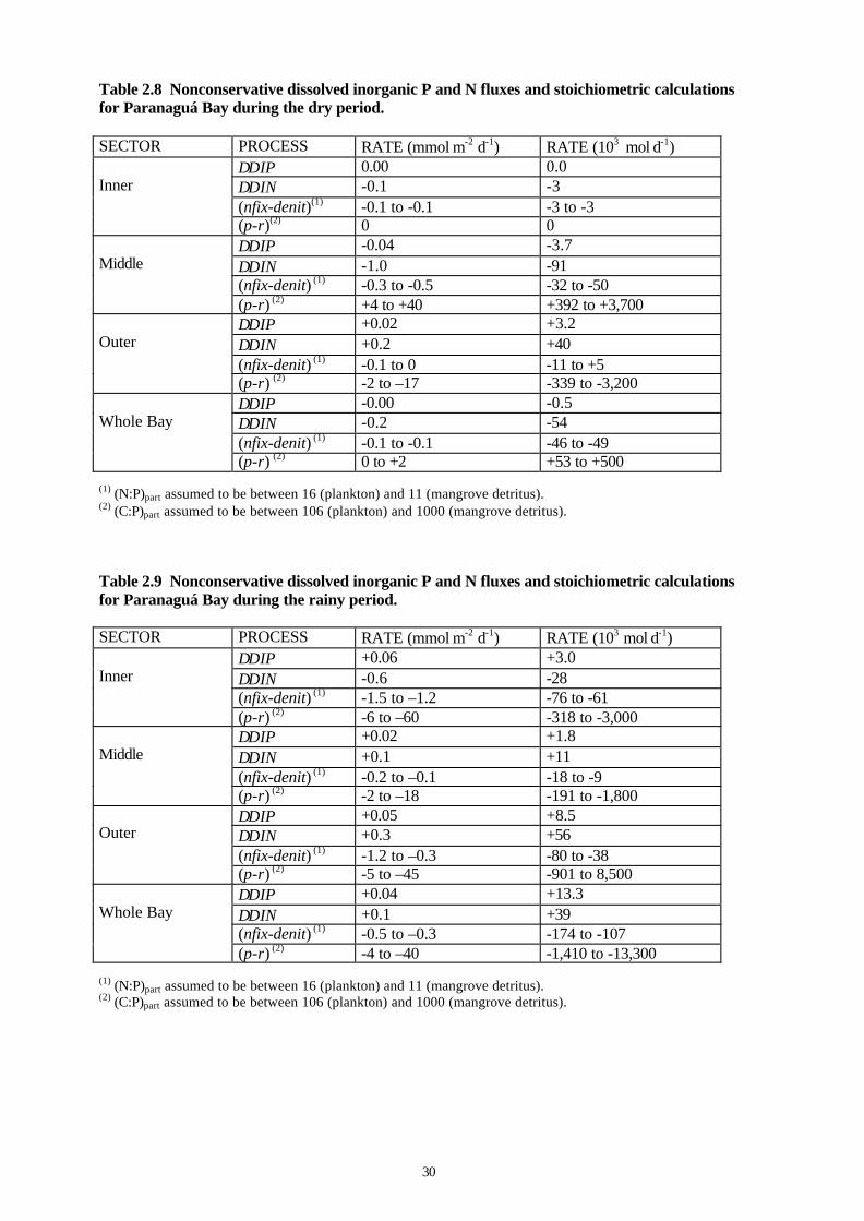
DIP balanceNonconservative fluxes of DIP are positive in the three sectors of Paranaguá Bay during the rainyseason, suggesting that there is a net production of DIP within the system in this season. During thedry season DIP fluxes are positive only in the outer sector, whereas the inner and middle sectors seemto be a net sink. On an annual basis and over the whole system, ∆DIP amounts to +2.3x106 mol P yr-1

or +7.0 mmol P m-2 yr-1. Assuming that phosphate desorption from sediments does not contributesubstantially to ∆DIP, then this DIP production is probably the result of net organic matter oxidation.Sewage discharge amounts to approximately 0.9x106 mol P yr-1. This accounts for 31% of theobserved non-conservative flux of DIP (∆DIP). The Paranaguá Port constitutes an additionalanthropogenic, non-quantified, source of P-fertilizers residues from charge and discharge operations.

DIN balanceThe picture is somewhat more complicated for DIN: the inner sector appears to be a net sink of DIN inboth periods, especially in the rainy season. On the other hand, nonconservative fluxes of DIN arepositive in the outer sector of the bay, both seasons, mainly in the rainy period. On an annual basisover the entire estuary, ∆DIN is -2.7x106 mol N yr-1 or -8 mmol m-2 yr-1, suggesting that netconsumption of DIN predominates.

Stoichiometric calculations of aspects of net system metabolismAlthough the DIP and DIN concentrations in the sections do not show significant differences betweenthe rainy to dry seasons, hydrographic fluxes are much higher during the rainy season. This is reflectedin the export of DIN and DIP to the adjacent coastal area. Nonconservative flux for DIP indicates lowuptake during the dry season, and high release during the wet season. ∆DIN switches from moderateuptake during the dry season to moderate release during the wet season.

Independent estimates suggest that organic metabolism in this system is dominated by plankton andmangrove detritus (Brandini 1985; Machado et al. in press). Stoichiometric calculations of nitrogenfixation - denitrification (nfix-denit) shown in Tables 2.8 and 2.9 are made from the differences

29

between observed and expected ∆DIN. The expected values of organic particle decomposition arebased on a range for N:P part between mangrove detritus (N:P part ≈ 11:1) and plankton (N:P part ≈ 16:1).Net denitrification predominates, with values between -24.3 to -10.6x106 mol N yr-1 or -0.07 to -0.03mol N m-2 yr-1. The exception is the middle sector of the bay during the rainy season, where nitrogenfixation surpasses denitrification. Although these rates are only rough estimates, they seem reasonable.

Moreover, these results are in agreement with early studies, which reported predominantly low N:Pratios, lower than the classical Redfield ratio, attributed to denitrification (Knoppers et al. 1987;Machado et al. in press). However, direct denitrification rate estimates are not available for ParanaguáBay.

Net ecosystem metabolism (NEM = [p-r]) can also be estimated from ∆DIP and C:P ratio of thereacting organic matter. For this calculation, we assume that the reacting organic matter is dominatedby plankton and mangrove detritus, with C:P ratios about 106:1 and 1000:1, respectively. On anannual sacale, this amounts to -2,300 to -244x106 mol C yr-1 or -7 to -0.7 mmol C m-2 yr-1), over thewhole system. With mangroves dominating the net metabolism, the rates of (p-r) seem to beexcessively high. This suggests that the net reacting matter is plankton, contradicting the earlierstudies cited above. In either case, if the stoichiometric assumptions are valid, Paranaguá Bay appearsto be net heterotrophic throughout the annual cycle, with higher net metabolic rates during the warmer,rainy season.

Table 2.7 Physical characteristics of inner, middle and outer sections of Paranaguá Bay.

SectorSectionArea(103m2)

Area

(106m2)

MeanDepth(m)

WaterVolume(106m3)

Runoff(106

m3day-1)Rainy Dry

TidalDischarge(m3 sec-1)

TidalPrism(106m3)

Inner 9 50 2 95 10* 3* 5,331 119Middle 50 93 4 400 7 2 7,885 176Outer 130 187 7 1,309 4 1 12,724 284

* Data calculated from Mantovanelli et al. 1999.

30

Table 2.8 Nonconservative dissolved inorganic P and N fluxes and stoichiometric calculationsfor Paranaguá Bay during the dry period.

SECTOR PROCESS RATE (mmol⋅m-2 ⋅d-1) RATE (103 mol⋅d-1)∆DIP 0.00 0.0∆DIN -0.1 -3(nfix-denit)(1) -0.1 to -0.1 -3 to -3

Inner

(p-r)(2) 0 0∆DIP -0.04 -3.7∆DIN -1.0 -91(nfix-denit) (1) -0.3 to -0.5 -32 to -50

Middle

(p-r) (2) +4 to +40 +392 to +3,700∆DIP +0.02 +3.2∆DIN +0.2 +40(nfix-denit) (1) -0.1 to 0 -11 to +5

Outer

(p-r) (2) -2 to –17 -339 to -3,200∆DIP -0.00 -0.5∆DIN -0.2 -54(nfix-denit) (1) -0.1 to -0.1 -46 to -49

Whole Bay

(p-r) (2) 0 to +2 +53 to +500

(1) (N:P)part assumed to be between 16 (plankton) and 11 (mangrove detritus).(2) (C:P)part assumed to be between 106 (plankton) and 1000 (mangrove detritus).

Table 2.9 Nonconservative dissolved inorganic P and N fluxes and stoichiometric calculationsfor Paranaguá Bay during the rainy period.

SECTOR PROCESS RATE (mmol⋅m-2 ⋅d-1) RATE (103 mol⋅d-1)∆DIP +0.06 +3.0∆DIN -0.6 -28(nfix-denit) (1) -1.5 to –1.2 -76 to -61

Inner

(p-r) (2) -6 to –60 -318 to -3,000∆DIP +0.02 +1.8∆DIN +0.1 +11(nfix-denit) (1) -0.2 to –0.1 -18 to -9

Middle

(p-r) (2) -2 to –18 -191 to -1,800∆DIP +0.05 +8.5∆DIN +0.3 +56(nfix-denit) (1) -1.2 to –0.3 -80 to -38

Outer

(p-r) (2) -5 to –45 -901 to 8,500∆DIP +0.04 +13.3∆DIN +0.1 +39(nfix-denit) (1) -0.5 to –0.3 -174 to -107

Whole Bay

(p-r) (2) -4 to –40 -1,410 to -13,300

(1) (N:P)part assumed to be between 16 (plankton) and 11 (mangrove detritus).(2) (C:P)part assumed to be between 106 (plankton) and 1000 (mangrove detritus).

31

Figure 2.25 Water and salt budgets for Paranaguá Bay in the dry season. Volume in 106

m3, water fluxes in 106 m3 day-1, salt fluxes in 109 psu-m3 day-1, salinity in psu and water exchangetime (ι) in days.

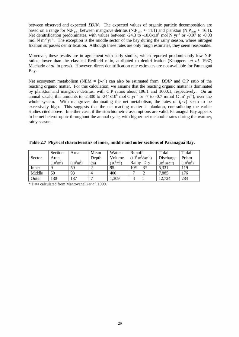
Figure 2.26 Water and salt budgets for Paranaguá Bay in the rainy season. Volume in 106

m3, water fluxes in 106 m3 day-1, salt fluxes in 109 psu-m3 day-1, salinity in psu and water exchangetime (ι) in days.

Figure 2.27 DIP budget for Paranaguá Bay in the dry season. Fluxes in 103 mol day-1 andconcentrations in mmol m-3.

Inner V1=95

S1=12.0 ττ 11=11

Middle V2=400 S2=22.0

ττ22=15

Outer V3=1,309 S3=30.0

τ τ 33=22

VR1 =3.1 VR2=5.1 VR3=5.8

VP1=0.1 VE1=0.2 VP2 =0.3 VE2=0.5 VP3 =0.8 VE3=1.3

VX1(S2-S1)= -VR1SR1=53 VX1 =5.3

VQ2=2 VG2=0.2

VQ3=1 VG3=0.2

VQ1=3 VG1=0.2

Socn=35

ττsyst =30

VX2(S3-S2)= -VR2SR2=133 VX2=16.6

VX3(Socn -S3)= -VR3SR3=189 VX3=37.7

Inner V1=95 S1=5.0

ττ 11=5

Middle V2=400 S2=18.0

ττ22=5

Outer V3=1,309 S3=27.0

ττ 33=8

VR1 =10.7 VR2=18.5 VR3=23.5

VP1=0.4 VE1 =0.3 VP2=0.9 VE2=0.7 VP3 = 2.2 VE3 = 1.8

VX1(S2-S1)= -VR1SR1=123 VX1=9.5

VQ2=7 VG2=0.6

VQ3 =4 VG3 = 0.6

VQ1=10 VG1=0.6

Socn=34

ττsyst =14

VX2(S3-S2)= -VR2SR2=416 VX2=46.3

VX3(Socn -S3)= -VR3SR3=717 VX3=102.4

Inner DIP1 = 0.9

∆∆DIP 1 1 = 0.0

Middle DIP2 = 0.8 ∆∆DIP2 = -3.7

Outer DIP3=0.6

∆∆DIP3=+3.2

VR1DIPR1

= 2.6

VX1(DIP2-DIP1) = 0.5

DIPQ1 = 0.7 VQ1DIPQ1 = 2.1

DIPocn = 0.4

∆∆DIPsyst = -0.5

VO1DIPO1

= 1.0

DIPQ2 = 0.7 VQ2DIPQ2 = 1.4

DIPQ3 = 0.3 VQ3DIPQ3 = 0.3

VR2DIPR2

= 3.6VR3DIPR3

= 2.9



VO1DIPO1

= 6.1VO1DIPO1

= 0

32

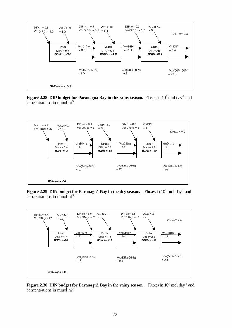
Figure 2.28 DIP budget for Paranaguá Bay in the rainy season. Fluxes in 103 mol day-1 andconcentrations in mmol m-3.

Figure 2.29 DIN budget for Paranaguá Bay in the dry season. Fluxes in 103 mol day-1 andconcentrations in mmol m-3.

Figure 2.30 DIN budget for Paranaguá Bay in the rainy season. Fluxes in 103 mol day-1 andconcentrations in mmol m-3.

Inner DIN1 = 6.7 ∆∆DIN 1 1 = -28

Middle DIN2 = 4.8

∆∆DIN 2 = +11

Outer DIN 3 = 2.3

∆∆DIN3 = +56

VR1DIN R1

= 62

VX1(DIN2-DIN1) = 18

DINQ1 = 9.7 VQ1DIN Q1 = 97

DINocn = 0.1

∆∆DIN syst = +39

VO1DIN O1

= 11

DIN Q2 = 3.0 VQ2DIN Q2 = 21

DIN Q3 = 3.8 VQ3 DINQ3 = 15

VR2DIN R2

= 66VR3DINR3

= 28



VO1 DINO1

= 70

VO1DINO1

= 0

Inner DIN 1 = 6.4

∆∆DIN 1 1 = -3

Middle DIN 2 = 2.9 ∆∆DIN2 = -91

Outer DIN 3 = 1.9

∆∆DIN3 = +40

VR1DINR1

= 14

VX1(DIN2-DIN1) = 19

DIN Q1 = 8.3 VQ1DINQ1 = 25

DINocn = 0.2

∆∆DIN syst = -54

VO1 DINO1

= 11

DIN Q2 = 8.6 VQ2DIN Q2 = 17

DIN Q3 = 0.8 VQ3DINQ3 = 1

VR2DINR2

= 12VR3DIN R3

= 6

VX2(DIN3-DIN2) = 17

VX3(DIN4-DIN3) = 64

VO1DIN O1

= 70

VO1DINO1

= 0

Inner DIP1 = 0.8

∆∆DIP1 1 = +3.0

Middle DIP2 = 0.7

∆∆DIP2 = +1.8

Outer DIP3=0.5

∆∆DIP3=+8.5

VR1DIPR1

= 8.0


DIPQ1 = 0.5 VQ1DIPQ1 = 5.0

DIPocn = 0.3

∆∆DIPsyst = +13.3

VO1DIPO1

= 1.0

DIPQ2 = 0.5 VQ2DIPQ2 = 3.5

DIPQ3 = 0.2 VQ3DIPQ3 = 1.0

VR2DIPR2

= 11.1VR3DIPR3

= 9.4


VX3(DIP4-DIP3) = 20.5

VO1DIPO1

= 6.1VO1DIPO1

= 0

33

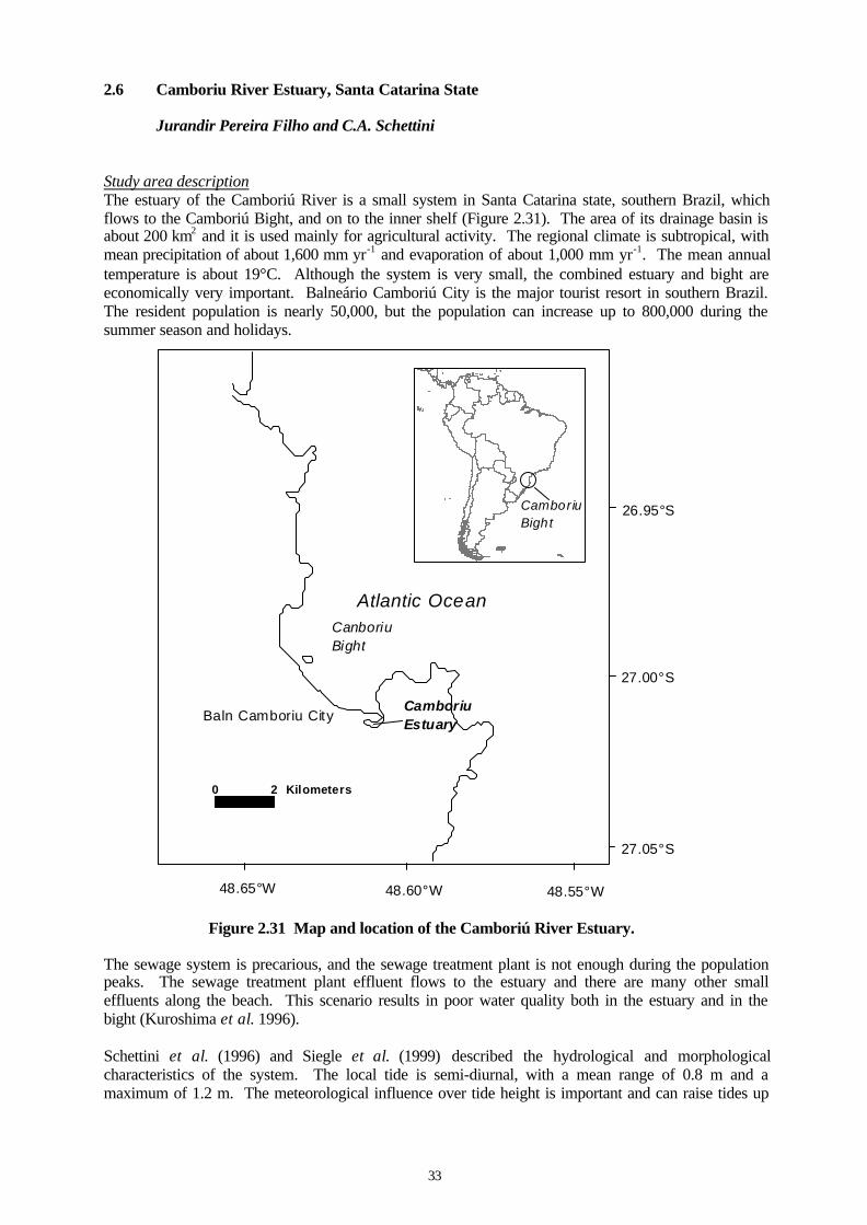
2.6 Camboriu River Estuary, Santa Catarina State

Jurandir Pereira Filho and C.A. Schettini

Study area descriptionThe estuary of the Camboriú River is a small system in Santa Catarina state, southern Brazil, whichflows to the Camboriú Bight, and on to the inner shelf (Figure 2.31). The area of its drainage basin isabout 200 km2 and it is used mainly for agricultural activity. The regional climate is subtropical, withmean precipitation of about 1,600 mm yr-1 and evaporation of about 1,000 mm yr-1. The mean annualtemperature is about 19°C. Although the system is very small, the combined estuary and bight areeconomically very important. Balneário Camboriú City is the major tourist resort in southern Brazil.The resident population is nearly 50,000, but the population can increase up to 800,000 during thesummer season and holidays.

Atlantic OceanCanboriuBight

#

CamboriuEstuaryBaln Camboriu City

27.05°S

27.00°S

26.95°S

48.55°W48.60°W48.65°W

0 2 Kilometers

CamboriuBight

Figure 2.31 Map and location of the Camboriú River Estuary.

The sewage system is precarious, and the sewage treatment plant is not enough during the populationpeaks. The sewage treatment plant effluent flows to the estuary and there are many other smalleffluents along the beach. This scenario results in poor water quality both in the estuary and in thebight (Kuroshima et al. 1996).

Schettini et al. (1996) and Siegle et al. (1999) described the hydrological and morphologicalcharacteristics of the system. The local tide is semi-diurnal, with a mean range of 0.8 m and amaximum of 1.2 m. The meteorological influence over tide height is important and can raise tides up

34

to 1 m above the astronomical tide (Schettini et al. 1996; Carvalho et al. 1996). The estimatedfreshwater inflow to the system is about 500,000 m3 day-1, on average. Siegle et al. (1996, 1998)classified the Camboriú River estuary as a shallow and partially mixed estuary. The water columnstratification is greater during neap tide conditions, whereas during spring tide condition the watercolumn is vertically almost homogeneous. The estuary is the main source of materials to the bight. Itschannel is about 120 m wide near the mouth and has a mean depth of 2 m. There are a few mangrovepatches around the inlet, but they are severely degraded.

Most of the bight has an homogeneous water column, but close to the estuarine mouth there is abuoyant plume that indicates local stratification. The Itajaí-açu River mouth is just 15 km to north, butits plume goes north and does not play an important role to the bight water quality, although it doesinfluence the inner shelf salinity (~ 33 psu).

A major project was carried out to evaluate the bight water quality, with 16 sampling stationsdistributed over the bight, surveyed monthly over a year in 1994 and 1995. This characterization wassummarized by Morelli (1997). Some minor projects were carried out in the estuary, and there is anongoing project with fortnightly sampling along the estuary (Kuroshima, unpublished data).Information from experiments over tidal cycles is also available after 1998 and was used in this workto characterize the estuary (Pereira Filho et al., unpublished data). The Camboriú River estuary budgetwas calculated using some of these data (Tables 2.10 and 2.11).

Table 2.10 Characteristics of the Camboriú River system.

Length 9,500 mMean Depth 2 mArea 0.5 km2

Volume 1 x 106 m3

System + Flood Plain 0.7 km2

Mean Discharge 500,000 m3 day-1

Table 2.11 Average salinity and nutrient concentrations of the Camboriú River system.

CamboriúRiver

Camboriú InnerEstuary

Camboriú OuterEstuary

CamboriúBight

Salinity (psu) 0.0 9.5 25 28.7DIP (mmol m-3) 0.5 0.7 0.4NO3

- (mmol m-3) 7.5 2.8 1.5

NO2- (mmol m-3) 0.3 1.0 0.2

NH4+

(mmol m-3) 10.4 29.7 10.0DIN (mmol m-3) 18.1 33.5 11.7

Source: Camboriú River-Kuroshima (unpublished data); Schettini et al. (1996) Camboriú Estuary- Pereira Filho et al. (in preparation) Camboriú Bight- Morelli (1997)

Water and salt balanceFigure 2.32 illustrates the water and salt budget for Camboriú River estuary. The budget wascalculated using LOICZ Biogeochemical Modelling Guidelines (Gordon et al. 1996). The riverdischarge (VQ) is based on Schettini et al. (1996). There are no data on groundwater discharge (VG)and we assume it to be zero. Direct rainfall and evaporation over the estuary are close to zero. Theresidual water flux to the Camboriú Bight (VR) is 500 x 103 m3 day-1. The average salinity in the innerestuary and in the Camboriú Bight is based on Schettini et al. (1996) and on Morelli (1997)respectively. The mixing flux (VX) calculated the Camboriú estuary and bight is 3,628x103 m3 day-1.Water exchange time (Vsyst/(VX + |VR|) is about 0.24 day.

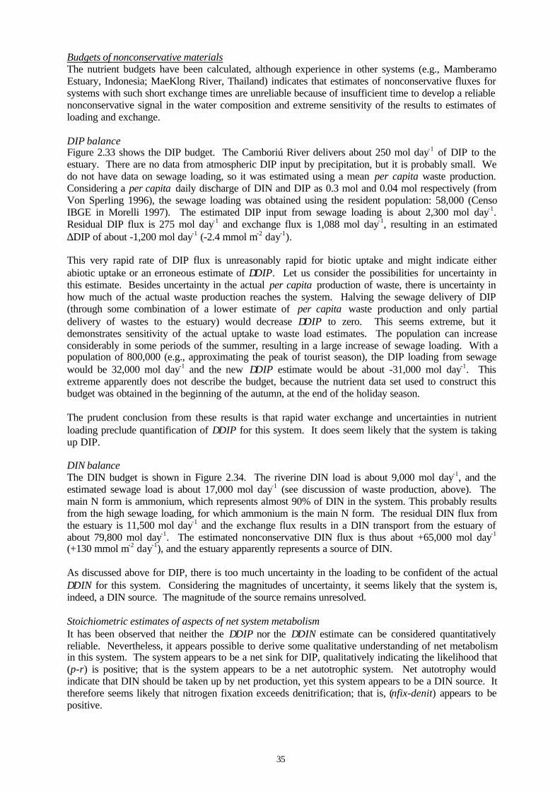
35

Budgets of nonconservative materialsThe nutrient budgets have been calculated, although experience in other systems (e.g., MamberamoEstuary, Indonesia; MaeKlong River, Thailand) indicates that estimates of nonconservative fluxes forsystems with such short exchange times are unreliable because of insufficient time to develop a reliablenonconservative signal in the water composition and extreme sensitivity of the results to estimates ofloading and exchange.

DIP balanceFigure 2.33 shows the DIP budget. The Camboriú River delivers about 250 mol day-1 of DIP to theestuary. There are no data from atmospheric DIP input by precipitation, but it is probably small. Wedo not have data on sewage loading, so it was estimated using a mean per capita waste production.Considering a per capita daily discharge of DIN and DIP as 0.3 mol and 0.04 mol respectively (fromVon Sperling 1996), the sewage loading was obtained using the resident population: 58,000 (CensoIBGE in Morelli 1997). The estimated DIP input from sewage loading is about 2,300 mol day-1.Residual DIP flux is 275 mol day-1 and exchange flux is 1,088 mol day-1, resulting in an estimated∆DIP of about -1,200 mol day-1 (-2.4 mmol m-2 day-1).

This very rapid rate of DIP flux is unreasonably rapid for biotic uptake and might indicate eitherabiotic uptake or an erroneous estimate of ∆DIP. Let us consider the possibilities for uncertainty inthis estimate. Besides uncertainty in the actual per capita production of waste, there is uncertainty inhow much of the actual waste production reaches the system. Halving the sewage delivery of DIP(through some combination of a lower estimate of per capita waste production and only partialdelivery of wastes to the estuary) would decrease ∆DIP to zero. This seems extreme, but itdemonstrates sensitivity of the actual uptake to waste load estimates. The population can increaseconsiderably in some periods of the summer, resulting in a large increase of sewage loading. With apopulation of 800,000 (e.g., approximating the peak of tourist season), the DIP loading from sewagewould be 32,000 mol day-1 and the new ∆DIP estimate would be about -31,000 mol day-1. Thisextreme apparently does not describe the budget, because the nutrient data set used to construct thisbudget was obtained in the beginning of the autumn, at the end of the holiday season.

The prudent conclusion from these results is that rapid water exchange and uncertainties in nutrientloading preclude quantification of ∆DIP for this system. It does seem likely that the system is takingup DIP.

DIN balanceThe DIN budget is shown in Figure 2.34. The riverine DIN load is about 9,000 mol day-1, and theestimated sewage load is about 17,000 mol day-1 (see discussion of waste production, above). Themain N form is ammonium, which represents almost 90% of DIN in the system. This probably resultsfrom the high sewage loading, for which ammonium is the main N form. The residual DIN flux fromthe estuary is 11,500 mol day-1 and the exchange flux results in a DIN transport from the estuary ofabout 79,800 mol day-1. The estimated nonconservative DIN flux is thus about +65,000 mol day-1

(+130 mmol m-2 day-1), and the estuary apparently represents a source of DIN.

As discussed above for DIP, there is too much uncertainty in the loading to be confident of the actual∆DIN for this system. Considering the magnitudes of uncertainty, it seems likely that the system is,indeed, a DIN source. The magnitude of the source remains unresolved.

Stoichiometric estimates of aspects of net system metabolismIt has been observed that neither the ∆DIP nor the ∆DIN estimate can be considered quantitativelyreliable. Nevertheless, it appears possible to derive some qualitative understanding of net metabolismin this system. The system appears to be a net sink for DIP, qualitatively indicating the likelihood that(p-r) is positive; that is the system appears to be a net autotrophic system. Net autotrophy wouldindicate that DIN should be taken up by net production, yet this system appears to be a DIN source. Ittherefore seems likely that nitrogen fixation exceeds denitrification; that is, (nfix-denit) appears to bepositive.

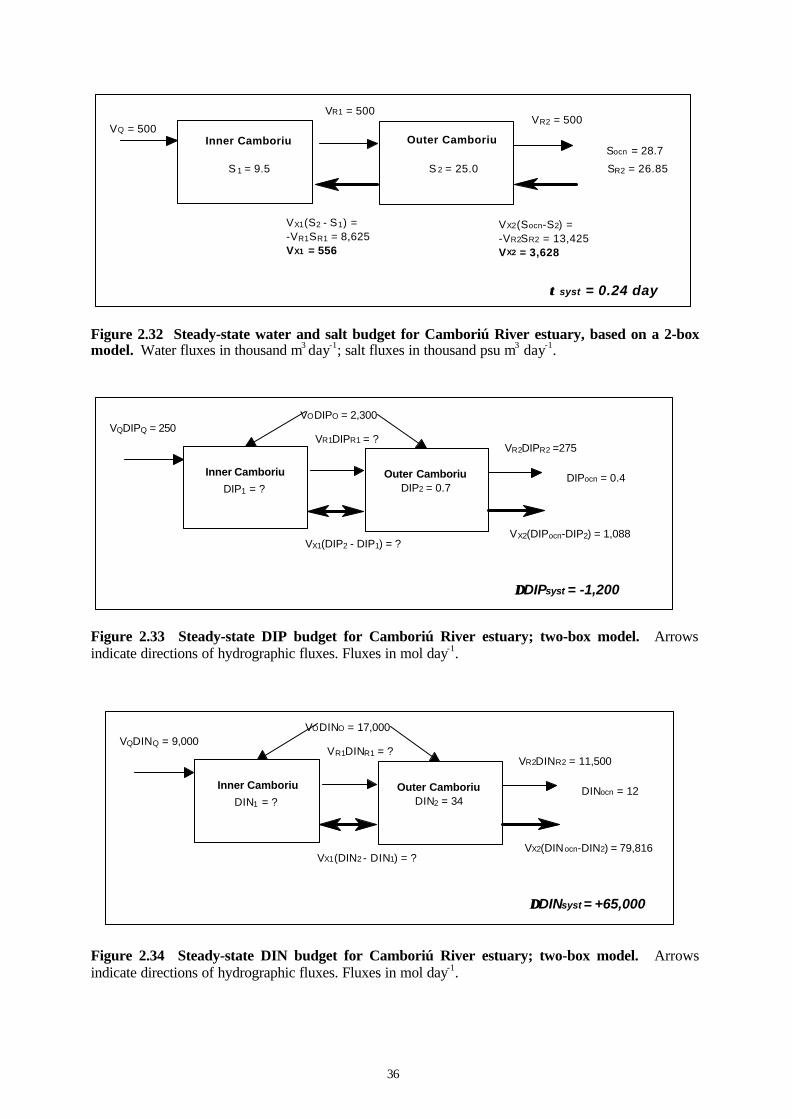
36

Figure 2.32 Steady-state water and salt budget for Camboriú River estuary, based on a 2-boxmodel. Water fluxes in thousand m3 day-1; salt fluxes in thousand psu m3 day-1.

Figure 2.33 Steady-state DIP budget for Camboriú River estuary; two-box model. Arrowsindicate directions of hydrographic fluxes. Fluxes in mol day-1.

Figure 2.34 Steady-state DIN budget for Camboriú River estuary; two-box model. Arrowsindicate directions of hydrographic fluxes. Fluxes in mol day-1.

Outer Camboriu DIN2 = 34

VQDINQ = 9,000

VR2DINR2 = 11,500

DINocn = 12

VX2(DINocn-DIN2) = 79,816

Inner Camboriu

DIN1 = ?

VX1(DIN2 - DIN1) = ?

VR1DINR1 = ?

VODINO = 17,000

∆∆DINsyst = +65,000

VQ = 500VR2 = 500

Socn = 28.7

SR2 = 26.85

VX2(Socn-S2) = -VR2SR2 = 13,425 VX2 = 3,628

VX1(S2 - S1) = -VR1SR1 = 8,625 VX1 = 556

VR1 = 500

τ τ syst = 0.24 day

Inner Camboriu

S 1 = 9.5

Outer Camboriu

S 2 = 25.0

Outer Camboriu DIP2 = 0.7

VQDIPQ = 250

VR2DIPR2 =275

DIPocn = 0.4

VX2(DIPocn-DIP2) = 1,088

Inner Camboriu

DIP1 = ?

VX1(DIP2 - DIP1) = ?

VR1DIPR1 = ?

VODIPO = 2,300

∆∆DIPsyst = -1,200

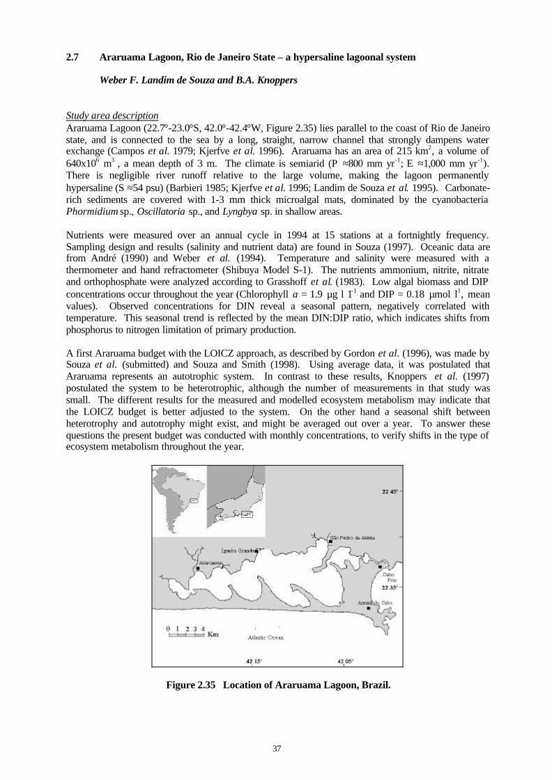
37

2.7 Araruama Lagoon, Rio de Janeiro State – a hypersaline lagoonal system

Weber F. Landim de Souza and B.A. Knoppers

Study area descriptionAraruama Lagoon (22.7°-23.0°S, 42.0°-42.4°W, Figure 2.35) lies parallel to the coast of Rio de Janeirostate, and is connected to the sea by a long, straight, narrow channel that strongly dampens waterexchange (Campos et al. 1979; Kjerfve et al. 1996). Araruama has an area of 215 km2, a volume of640x106 m3 , a mean depth of 3 m. The climate is semiarid (P ≈800 mm yr-1; E ≈1,000 mm yr-1).There is negligible river runoff relative to the large volume, making the lagoon permanentlyhypersaline (S ≈54 psu) (Barbieri 1985; Kjerfve et al. 1996; Landim de Souza et al. 1995). Carbonate-rich sediments are covered with 1-3 mm thick microalgal mats, dominated by the cyanobacteriaPhormidium sp., Oscillatoria sp., and Lyngbya sp. in shallow areas.

Nutrients were measured over an annual cycle in 1994 at 15 stations at a fortnightly frequency.Sampling design and results (salinity and nutrient data) are found in Souza (1997). Oceanic data arefrom André (1990) and Weber et al. (1994). Temperature and salinity were measured with athermometer and hand refractometer (Shibuya Model S-1). The nutrients ammonium, nitrite, nitrateand orthophosphate were analyzed according to Grasshoff et al. (1983). Low algal biomass and DIPconcentrations occur throughout the year (Chlorophyll a = 1.9 µg l 1-1 and DIP = 0.18 µmol l-1, meanvalues). Observed concentrations for DIN reveal a seasonal pattern, negatively correlated withtemperature. This seasonal trend is reflected by the mean DIN:DIP ratio, which indicates shifts fromphosphorus to nitrogen limitation of primary production.

A first Araruama budget with the LOICZ approach, as described by Gordon et al. (1996), was made bySouza et al. (submitted) and Souza and Smith (1998). Using average data, it was postulated thatAraruama represents an autotrophic system. In contrast to these results, Knoppers et al. (1997)postulated the system to be heterotrophic, although the number of measurements in that study wassmall. The different results for the measured and modelled ecosystem metabolism may indicate thatthe LOICZ budget is better adjusted to the system. On the other hand a seasonal shift betweenheterotrophy and autotrophy might exist, and might be averaged out over a year. To answer thesequestions the present budget was conducted with monthly concentrations, to verify shifts in the type ofecosystem metabolism throughout the year.

Figure 2.35 Location of Araruama Lagoon, Brazil.

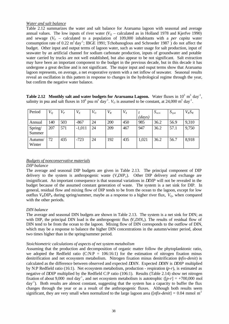
38

Water and salt balanceTable 2.12 summarizes the water and salt balance for Araruama lagoon with seasonal and averageannual values. The low inputs of river water (VQ – calculated as in Holland 1978 and Kjerfve 1990)and sewage (VO – calculated to a population of 109,000 inhabitants with a per capita waterconsumption rate of 0.22 m3 day-1; IBGE 1991; Tchobanoglous and Schroeder 1987 ) do not affect thebudget. Other input and output terms of lagoon water, such as water usage for salt production, input ofseawater by an artificial channel for sodium carbonate production, inputs of groundwater and potablewater carried by trucks are not well established, but also appear to be not significant. Salt extractionmay have been an important component to the budget in the previous decade, but in this decade it hasundergone a great decline and is not significant. The major input and ouput terms show that Araruamalagoon represents, on average, a net evaporative system with a net inflow of seawater. Seasonal resultsreveal an oscillation in this pattern in response to changes in the hydrological regime through the year,but confirm the negative water balance.

Table 2.12 Monthly salt and water budgets for Araruama Lagoon. Water fluxes in 103 m3 day-1,salinity in psu and salt fluxes in 106 psu m3 day-1. VO is assumed to be constant, at 24,000 m3 day-1.

Period VQ VP VE VO VR VX τ(days)

Socn Ssyst VRSR

Annual 140 503 -867 24 200 450 985 36.2 56.9 9,310Spring/Summer

207 571 -1,011 24 209 467 947 36.2 57.1 9,750

Autumn/Winter

72 435 -723 24 192 435 1,021 36.2 56.7 8,918

Budgets of nonconservative materialsDIP balanceThe average and seasonal DIP budgets are given in Table 2.13. The principal component of DIPdelivery to the system is anthropogenic waste (VoDIPo). Other DIP delivery and exchange areinsignificant. An important consequence is that seasonal variations in ∆DIP will not be revealed in thebudget because of the assumed constant generation of waste. The system is a net sink for DIP. Ingeneral, residual flow and mixing flow of DIP tends to be from the ocean to the lagoon, except for lowoutflux VRDIPR during spring/summer, maybe as a response to a higher river flux, VQ, when comparedwith the other periods.

DIN balanceThe average and seasonal DIN budgets are shown in Table 2.13. The system is a net sink for DIN; aswith DIP, the principal DIN load is the anthropogenic flux (VoDINo). The results of residual flow ofDIN tend to be from the ocean to the lagoon. Mixing flow of DIN corresponds to the outflow of DIN,which may be a response to balance the higher DIN concentrations in the autumn/winter period, abouttwo times higher than in the spring/summer period.

Stoichiometric calculations of aspects of net system metabolismAssuming that the production and decomposition of organic matter follow the phytoplanktonic ratio,we adopted the Redfield ratio (C:N:P = 106:16:1) for the estimation of nitrogen fixation minusdenitrification and net ecosystem metabolism. Nitrogen fixation minus denitrification (nfix-denit) iscalculated as the difference between observed and expected ∆DIN. Expected ∆DIN is ∆DIP multipliedby N:P Redfield ratio (16:1). Net ecosystem metabolism, production - respiration (p-r), is estimated asnegative of ∆DIP multiplied by the Redfield C:P ratio (106:1). Results (Table 2.14) show net nitrogenfixation of about 9,000 mol day-1 , and net ecosystem metabolism is autotrophic ([p-r] = +700,000 molday-1). Both results are almost constant, suggesting that the system has a capacity to buffer the fluxchanges through the year or as a result of the anthropogenic fluxes. Although both results seemsignificant, they are very small when normalized to the large lagoon area ([nfix-denit] = 0.04 mmol m-2

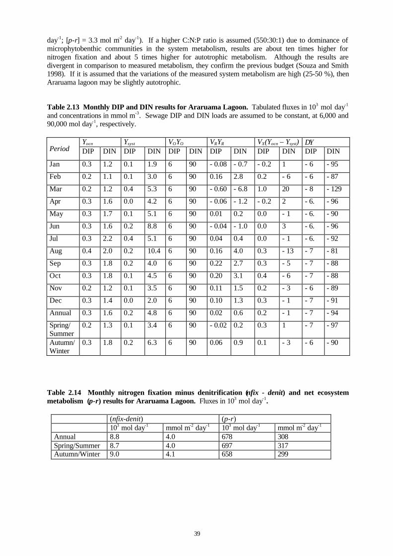
39

day-1; [p-r] = 3.3 mol m-2 day-1). If a higher C:N:P ratio is assumed (550:30:1) due to dominance ofmicrophytobenthic communities in the system metabolism, results are about ten times higher fornitrogen fixation and about 5 times higher for autotrophic metabolism. Although the results aredivergent in comparison to measured metabolism, they confirm the previous budget (Souza and Smith1998). If it is assumed that the variations of the measured system metabolism are high (25-50 %), thenAraruama lagoon may be slightly autotrophic.

Table 2.13 Monthly DIP and DIN results for Araruama Lagoon. Tabulated fluxes in 103 mol day-1

and concentrations in mmol m-3. Sewage DIP and DIN loads are assumed to be constant, at 6,000 and90,000 mol day-1, respectively.

Yocn Ysyst VOYO VRYR VX(Yocn – Ysyst) ∆YPeriod DIP DIN DIP DIN DIP DIN DIP DIN DIP DIN DIP DIN

Jan 0.3 1.2 0.1 1.9 6 90 - 0.08 - 0.7 - 0.2 1 - 6 - 95

Feb 0.2 1.1 0.1 3.0 6 90 0.16 2.8 0.2 - 6 - 6 - 87

Mar 0.2 1.2 0.4 5.3 6 90 - 0.60 - 6.8 1.0 20 - 8 - 129

Apr 0.3 1.6 0.0 4.2 6 90 - 0.06 - 1.2 - 0.2 2 - 6. - 96

May 0.3 1.7 0.1 5.1 6 90 0.01 0.2 0.0 - 1 - 6. - 90

Jun 0.3 1.6 0.2 8.8 6 90 - 0.04 - 1.0 0.0 3 - 6. - 96

Jul 0.3 2.2 0.4 5.1 6 90 0.04 0.4 0.0 - 1 - 6. - 92

Aug 0.4 2.0 0.2 10.4 6 90 0.16 4.0 0.3 - 13 - 7 - 81

Sep 0.3 1.8 0.2 4.0 6 90 0.22 2.7 0.3 - 5 - 7 - 88

Oct 0.3 1.8 0.1 4.5 6 90 0.20 3.1 0.4 - 6 - 7 - 88

Nov 0.2 1.2 0.1 3.5 6 90 0.11 1.5 0.2 - 3 - 6 - 89

Dec 0.3 1.4 0.0 2.0 6 90 0.10 1.3 0.3 - 1 - 7 - 91

Annual 0.3 1.6 0.2 4.8 6 90 0.02 0.6 0.2 - 1 - 7 - 94

Spring/Summer

0.2 1.3 0.1 3.4 6 90 - 0.02 0.2 0.3 1 - 7 - 97

Autumn/Winter

0.3 1.8 0.2 6.3 6 90 0.06 0.9 0.1 - 3 - 6 - 90

Table 2.14 Monthly nitrogen fixation minus denitrification (nfix - denit) and net ecosystemmetabolism (p-r) results for Araruama Lagoon. Fluxes in 103 mol day-1.

(nfix-denit) (p-r)103 mol day-1 mmol m-2 day-1 103 mol day-1 mmol m-2 day-1

Annual 8.8 4.0 678 308Spring/Summer 8.7 4.0 697 317Autumn/Winter 9.0 4.1 658 299

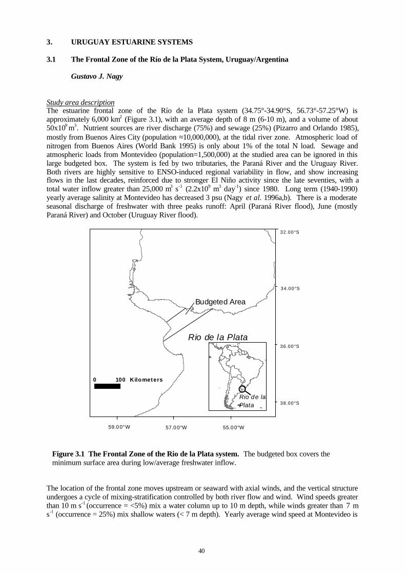
40

3. URUGUAY ESTUARINE SYSTEMS

3.1 The Frontal Zone of the Río de la Plata System, Uruguay/Argentina

Gustavo J. Nagy

Study area descriptionThe estuarine frontal zone of the Río de la Plata system (34.75°-34.90°S, 56.73°-57.25°W) isapproximately 6,000 km2 (Figure 3.1), with an average depth of 8 m (6-10 m), and a volume of about50x109 m3. Nutrient sources are river discharge (75%) and sewage (25%) (Pizarro and Orlando 1985),mostly from Buenos Aires City (population ≈10,000,000), at the tidal river zone. Atmospheric load ofnitrogen from Buenos Aires (World Bank 1995) is only about 1% of the total N load. Sewage andatmospheric loads from Montevideo (population=1,500,000) at the studied area can be ignored in thislarge budgeted box. The system is fed by two tributaries, the Paraná River and the Uruguay River.Both rivers are highly sensitive to ENSO-induced regional variability in flow, and show increasingflows in the last decades, reinforced due to stronger El Niño activity since the late seventies, with atotal water inflow greater than 25,000 m3 s-1 (2.2x109 m3 day-1) since 1980. Long term (1940-1990)yearly average salinity at Montevideo has decreased 3 psu (Nagy et al. 1996a,b). There is a moderateseasonal discharge of freshwater with three peaks runoff: April (Paraná River flood), June (mostlyParaná River) and October (Uruguay River flood).

Rio de la Plata

32.00°S

34.00°S

36.00°S

38.00°S

59.0 0°W 57.0 0°W 55.0 0°W

#

Budgeted Area

0 100 Kilometers

Rio de laPlata

The location of the frontal zone moves upstream or seaward with axial winds, and the vertical structureundergoes a cycle of mixing-stratification controlled by both river flow and wind. Wind speeds greaterthan 10 m s-1 (occurrence = <5%) mix a water column up to 10 m depth, while winds greater than 7 ms-1 (occurrence = 25%) mix shallow waters (< 7 m depth). Yearly average wind speed at Montevideo is

Figure 3.1 The Frontal Zone of the Rio de la Plata system. The budgeted box covers theminimum surface area during low/average freshwater inflow.

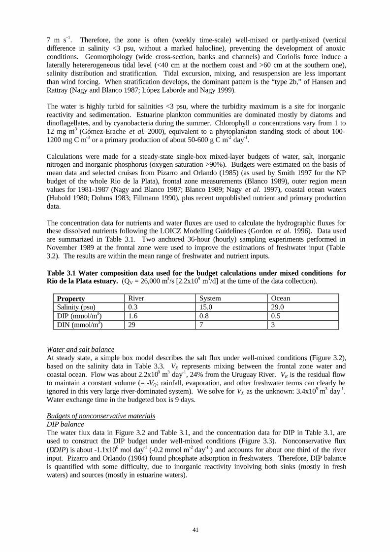
41

7 m s-1. Therefore, the zone is often (weekly time-scale) well-mixed or partly-mixed (verticaldifference in salinity <3 psu, without a marked halocline), preventing the development of anoxicconditions. Geomorphology (wide cross-section, banks and channels) and Coriolis force induce alaterally hetererogeneous tidal level (<40 cm at the northern coast and >60 cm at the southern one),salinity distribution and stratification. Tidal excursion, mixing, and resuspension are less importantthan wind forcing. When stratification develops, the dominant pattern is the “type 2b,” of Hansen andRattray (Nagy and Blanco 1987; López Laborde and Nagy 1999).

The water is highly turbid for salinities <3 psu, where the turbidity maximum is a site for inorganicreactivity and sedimentation. Estuarine plankton communities are dominated mostly by diatoms anddinoflagellates, and by cyanobacteria during the summer. Chlorophyll a concentrations vary from 1 to12 mg m-3 (Gómez-Erache et al. 2000), equivalent to a phytoplankton standing stock of about 100-1200 mg C m-3 or a primary production of about 50-600 g C m-2 day-1.

Calculations were made for a steady-state single-box mixed-layer budgets of water, salt, inorganicnitrogen and inorganic phosphorus (oxygen saturation >90%). Budgets were estimated on the basis ofmean data and selected cruises from Pizarro and Orlando (1985) (as used by Smith 1997 for the NPbudget of the whole Rio de la Plata), frontal zone measurements (Blanco 1989), outer region meanvalues for 1981-1987 (Nagy and Blanco 1987; Blanco 1989; Nagy et al. 1997), coastal ocean waters(Hubold 1980; Dohms 1983; Fillmann 1990), plus recent unpublished nutrient and primary productiondata.

The concentration data for nutrients and water fluxes are used to calculate the hydrographic fluxes forthese dissolved nutrients following the LOICZ Modelling Guidelines (Gordon et al. 1996). Data usedare summarized in Table 3.1. Two anchored 36-hour (hourly) sampling experiments performed inNovember 1989 at the frontal zone were used to improve the estimations of freshwater input (Table3.2). The results are within the mean range of freshwater and nutrient inputs.

Table 3.1 Water composition data used for the budget calculations under mixed conditions forRio de la Plata estuary. (QV = 26,000 m3/s [2.2x109 m3/d] at the time of the data collection).

Property River System OceanSalinity (psu) 0.3 15.0 29.0DIP (mmol/m3) 1.6 0.8 0.5DIN (mmol/m3) 29 7 3

Water and salt balanceAt steady state, a simple box model describes the salt flux under well-mixed conditions (Figure 3.2),based on the salinity data in Table 3.3. VX represents mixing between the frontal zone water andcoastal ocean. Flow was about 2.2x109 m3 day-1, 24% from the Uruguay River. VR is the residual flowto maintain a constant volume (= -VQ; rainfall, evaporation, and other freshwater terms can clearly beignored in this very large river-dominated system). We solve for VX as the unknown: 3.4x109 m3 day-1.Water exchange time in the budgeted box is 9 days.

Budgets of nonconservative materialsDIP balanceThe water flux data in Figure 3.2 and Table 3.1, and the concentration data for DIP in Table 3.1, areused to construct the DIP budget under well-mixed conditions (Figure 3.3). Nonconservative flux(∆DIP) is about -1.1x106 mol day-1 (-0.2 mmol m-2 day-1 ) and accounts for about one third of the riverinput. Pizarro and Orlando (1984) found phosphate adsorption in freshwaters. Therefore, DIP balanceis quantified with some difficulty, due to inorganic reactivity involving both sinks (mostly in freshwaters) and sources (mostly in estuarine waters).

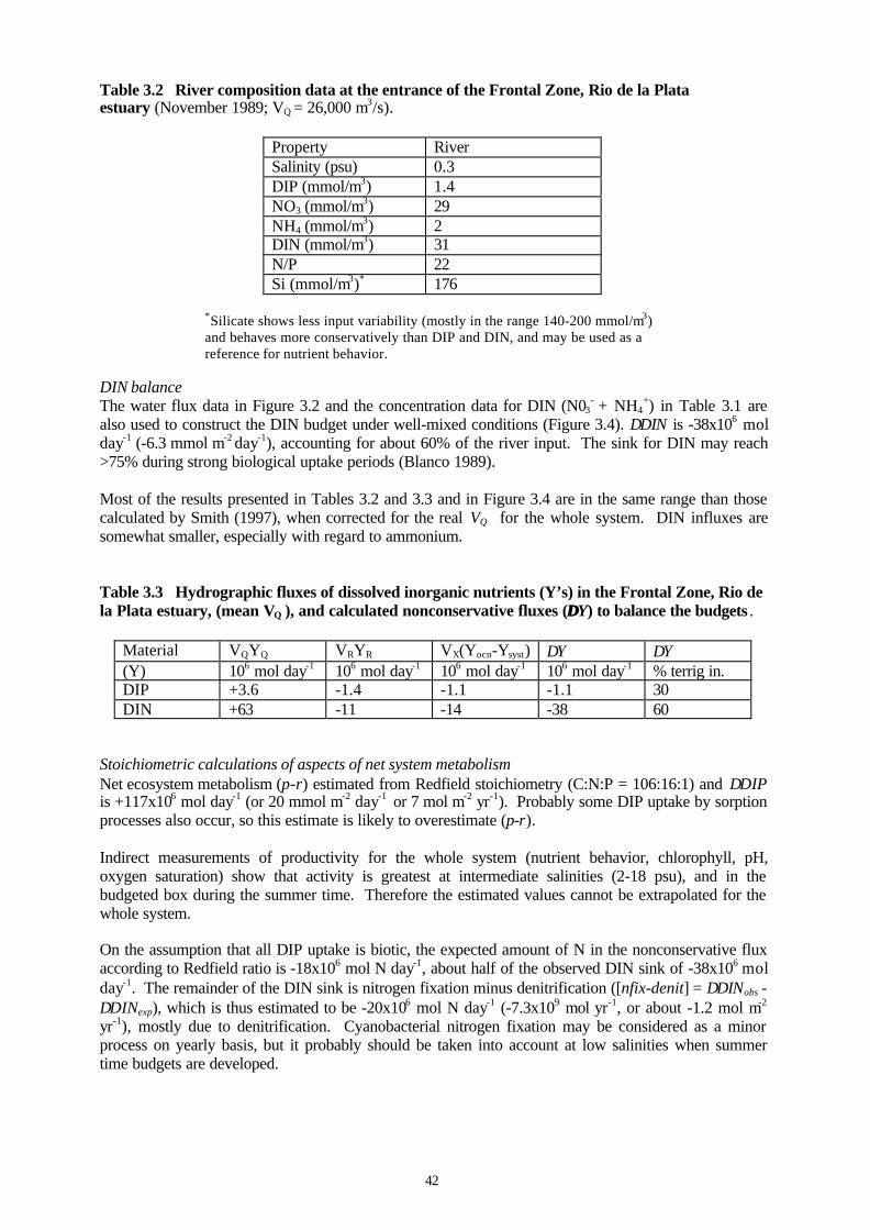
42

Table 3.2 River composition data at the entrance of the Frontal Zone, Rio de la Plataestuary (November 1989; VQ = 26,000 m3/s).

Property RiverSalinity (psu) 0.3DIP (mmol/m3) 1.4NO3 (mmol/m3) 29NH4 (mmol/m3) 2DIN (mmol/m3) 31N/P 22Si (mmol/m3)* 176

*Silicate shows less input variability (mostly in the range 140-200 mmol/m3)and behaves more conservatively than DIP and DIN, and may be used as areference for nutrient behavior.

DIN balanceThe water flux data in Figure 3.2 and the concentration data for DIN (N03

- + NH4+) in Table 3.1 are

also used to construct the DIN budget under well-mixed conditions (Figure 3.4). ∆DIN is -38x106 molday-1 (-6.3 mmol m-2 day-1), accounting for about 60% of the river input. The sink for DIN may reach>75% during strong biological uptake periods (Blanco 1989).

Most of the results presented in Tables 3.2 and 3.3 and in Figure 3.4 are in the same range than thosecalculated by Smith (1997), when corrected for the real VQ for the whole system. DIN influxes aresomewhat smaller, especially with regard to ammonium.

Table 3.3 Hydrographic fluxes of dissolved inorganic nutrients (Y’s) in the Frontal Zone, Rio dela Plata estuary, (mean VQ ), and calculated nonconservative fluxes (∆∆Y) to balance the budgets .

Material VQYQ VRYR VX(Yocn-Ysyst) ∆Y ∆Y(Y) 106 mol day-1 106 mol day-1 106 mol day-1 106 mol day-1 % terrig in.DIP +3.6 -1.4 -1.1 -1.1 30DIN +63 -11 -14 -38 60

Stoichiometric calculations of aspects of net system metabolismNet ecosystem metabolism (p-r) estimated from Redfield stoichiometry (C:N:P = 106:16:1) and ∆DIPis +117x106 mol day-1 (or 20 mmol m-2 day-1 or 7 mol m-2 yr-1). Probably some DIP uptake by sorptionprocesses also occur, so this estimate is likely to overestimate (p-r).

Indirect measurements of productivity for the whole system (nutrient behavior, chlorophyll, pH,oxygen saturation) show that activity is greatest at intermediate salinities (2-18 psu), and in thebudgeted box during the summer time. Therefore the estimated values cannot be extrapolated for thewhole system.

On the assumption that all DIP uptake is biotic, the expected amount of N in the nonconservative fluxaccording to Redfield ratio is -18x106 mol N day-1, about half of the observed DIN sink of -38x106 molday-1. The remainder of the DIN sink is nitrogen fixation minus denitrification ([nfix-denit] = ∆DINobs -∆DINexp), which is thus estimated to be -20x106 mol N day-1 (-7.3x109 mol yr-1, or about -1.2 mol m-2

yr-1), mostly due to denitrification. Cyanobacterial nitrogen fixation may be considered as a minorprocess on yearly basis, but it probably should be taken into account at low salinities when summertime budgets are developed.

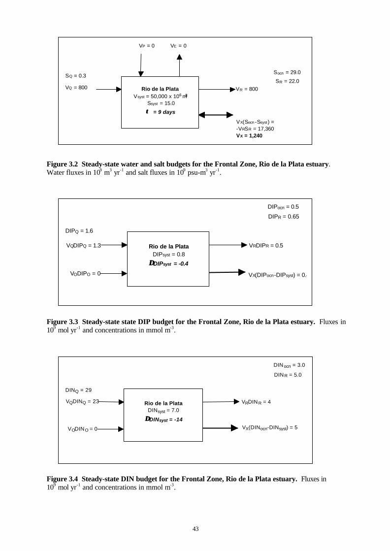
43

Figure 3.2 Steady-state water and salt budgets for the Frontal Zone, Rio de la Plata estuary.Water fluxes in 109 m3 yr-1 and salt fluxes in 109 psu-m3 yr-1.

Figure 3.3 Steady-state state DIP budget for the Frontal Zone, Rio de la Plata estuary. Fluxes in109 mol yr-1 and concentrations in mmol m-3.

Figure 3.4 Steady-state DIN budget for the Frontal Zone, Rio de la Plata estuary. Fluxes in109 mol yr-1 and concentrations in mmol m-3.

Rio de la Plata DIPsyst = 0.8


VQDIPQ = 1.3 VRDIPR = 0.5

DIPocn = 0.5

DIPR = 0.65

VX(DIPocn-DIPsyst) = 0.4VODIPO = 0

DIPQ = 1.6

Rio de la Plata DINsyst = 7.0

∆∆DINsyst = -14


DINocn = 3.0

DINR = 5.0


DINQ = 29

Rio de la Plata Vsyst = 50,000 x 10 m

Ssyst = 15.0

τ τ = 9 days

VP = 0 VE = 0

VQ = 800 VR = 800

Socn = 29.0

SR = 22.0

VX(Socn -Ssyst) = -VRSR = 17,360 VX = 1,240

6

SQ = 0.3

3

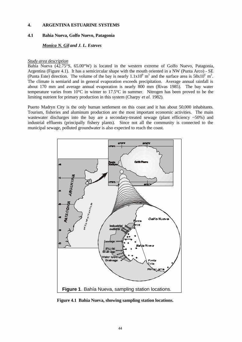
44

4. ARGENTINA ESTUARINE SYSTEMS

4.1 Bahia Nueva, Golfo Nuevo, Patagonia

Monica N. Gil and J. L. Esteves

Study area descriptionBahía Nueva (42.75°S, 65.00°W) is located in the western extreme of Golfo Nuevo, Patagonia,Argentina (Figure 4.1). It has a semicircular shape with the mouth oriented in a NW (Punta Arco) - SE(Punta Este) direction. The volume of the bay is nearly 1.1x109 m3 and the surface area is 58x106 m2.The climate is semiarid and in general evaporation exceeds precipitation. Average annual rainfall isabout 170 mm and average annual evaporation is nearly 800 mm (Rivas 1985). The bay watertemperature varies from 10°C in winter to 17.5°C in summer. Nitrogen has been proved to be thelimiting nutrient for primary production in this system (Charpy et al. 1982).

Puerto Madryn City is the only human settlement on this coast and it has about 50,000 inhabitants.Tourism, fisheries and aluminum production are the most important economic activities. The mainwastewater discharges into the bay are a secondary-treated sewage (plant efficiency ~50%) andindustrial effluents (principally fishery plants). Since not all the community is connected to themunicipal sewage, polluted groundwater is also expected to reach the coast.

Figure 4.1 Bahia Nueva, showing sampling station locations.

Figure 1. Bahía Nueva, sampling station locations.

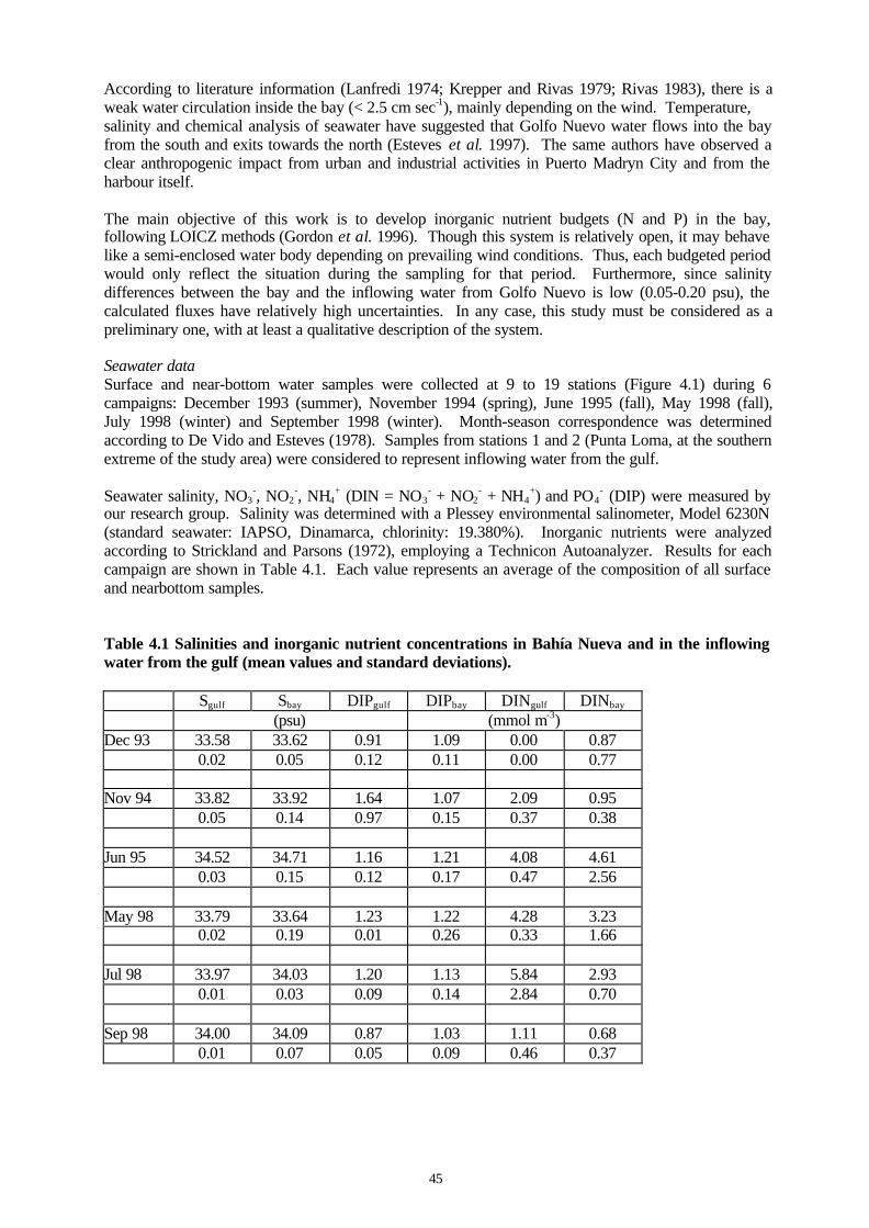
45

According to literature information (Lanfredi 1974; Krepper and Rivas 1979; Rivas 1983), there is aweak water circulation inside the bay (< 2.5 cm sec-1), mainly depending on the wind. Temperature,salinity and chemical analysis of seawater have suggested that Golfo Nuevo water flows into the bayfrom the south and exits towards the north (Esteves et al. 1997). The same authors have observed aclear anthropogenic impact from urban and industrial activities in Puerto Madryn City and from theharbour itself.

The main objective of this work is to develop inorganic nutrient budgets (N and P) in the bay,following LOICZ methods (Gordon et al. 1996). Though this system is relatively open, it may behavelike a semi-enclosed water body depending on prevailing wind conditions. Thus, each budgeted periodwould only reflect the situation during the sampling for that period. Furthermore, since salinitydifferences between the bay and the inflowing water from Golfo Nuevo is low (0.05-0.20 psu), thecalculated fluxes have relatively high uncertainties. In any case, this study must be considered as apreliminary one, with at least a qualitative description of the system.

Seawater dataSurface and near-bottom water samples were collected at 9 to 19 stations (Figure 4.1) during 6campaigns: December 1993 (summer), November 1994 (spring), June 1995 (fall), May 1998 (fall),July 1998 (winter) and September 1998 (winter). Month-season correspondence was determinedaccording to De Vido and Esteves (1978). Samples from stations 1 and 2 (Punta Loma, at the southernextreme of the study area) were considered to represent inflowing water from the gulf.

Seawater salinity, NO3-, NO2

-, NH4+ (DIN = NO3

- + NO2- + NH4

+) and PO4- (DIP) were measured by

our research group. Salinity was determined with a Plessey environmental salinometer, Model 6230N(standard seawater: IAPSO, Dinamarca, chlorinity: 19.380%). Inorganic nutrients were analyzedaccording to Strickland and Parsons (1972), employing a Technicon Autoanalyzer. Results for eachcampaign are shown in Table 4.1. Each value represents an average of the composition of all surfaceand nearbottom samples.

Table 4.1 Salinities and inorganic nutrient concentrations in Bahía Nueva and in the inflowingwater from the gulf (mean values and standard deviations).

Sgulf Sbay DIPgulf DIPbay DINgulf DINbay

(psu) (mmol m-3)Dec 93 33.58 33.62 0.91 1.09 0.00 0.87

0.02 0.05 0.12 0.11 0.00 0.77

Nov 94 33.82 33.92 1.64 1.07 2.09 0.950.05 0.14 0.97 0.15 0.37 0.38

Jun 95 34.52 34.71 1.16 1.21 4.08 4.610.03 0.15 0.12 0.17 0.47 2.56

May 98 33.79 33.64 1.23 1.22 4.28 3.230.02 0.19 0.01 0.26 0.33 1.66

Jul 98 33.97 34.03 1.20 1.13 5.84 2.930.01 0.03 0.09 0.14 2.84 0.70

Sep 98 34.00 34.09 0.87 1.03 1.11 0.680.01 0.07 0.05 0.09 0.46 0.37

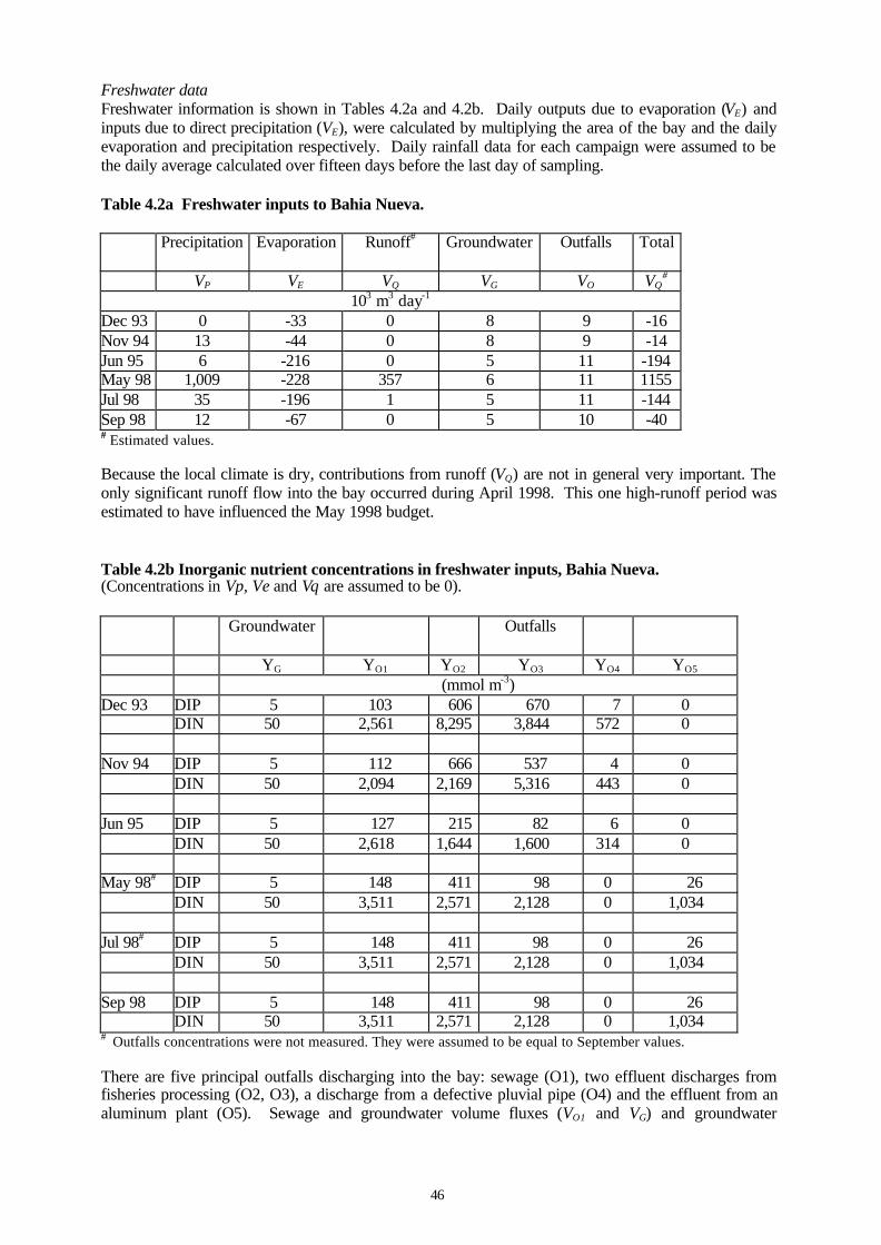
46

Freshwater dataFreshwater information is shown in Tables 4.2a and 4.2b. Daily outputs due to evaporation (VE) andinputs due to direct precipitation (VE), were calculated by multiplying the area of the bay and the dailyevaporation and precipitation respectively. Daily rainfall data for each campaign were assumed to bethe daily average calculated over fifteen days before the last day of sampling.

Table 4.2a Freshwater inputs to Bahia Nueva.

Precipitation Evaporation Runoff# Groundwater Outfalls Total

VP VE VQ VG VO VQ#

103 m3 day-1

Dec 93 0 -33 0 8 9 -16Nov 94 13 -44 0 8 9 -14Jun 95 6 -216 0 5 11 -194May 98 1,009 -228 357 6 11 1155Jul 98 35 -196 1 5 11 -144Sep 98 12 -67 0 5 10 -40# Estimated values.

Because the local climate is dry, contributions from runoff (VQ) are not in general very important. Theonly significant runoff flow into the bay occurred during April 1998. This one high-runoff period wasestimated to have influenced the May 1998 budget.

Table 4.2b Inorganic nutrient concentrations in freshwater inputs, Bahia Nueva.(Concentrations in Vp, Ve and Vq are assumed to be 0).

Groundwater Outfalls

YG YO1 YO2 YO3 YO4 YO5

(mmol m-3)Dec 93 DIP 5 103 606 670 7 0

DIN 50 2,561 8,295 3,844 572 0

Nov 94 DIP 5 112 666 537 4 0DIN 50 2,094 2,169 5,316 443 0

Jun 95 DIP 5 127 215 82 6 0DIN 50 2,618 1,644 1,600 314 0

May 98# DIP 5 148 411 98 0 26DIN 50 3,511 2,571 2,128 0 1,034

Jul 98# DIP 5 148 411 98 0 26DIN 50 3,511 2,571 2,128 0 1,034

Sep 98 DIP 5 148 411 98 0 26DIN 50 3,511 2,571 2,128 0 1,034

# Outfalls concentrations were not measured. They were assumed to be equal to September values.

There are five principal outfalls discharging into the bay: sewage (O1), two effluent discharges fromfisheries processing (O2, O3), a discharge from a defective pluvial pipe (O4) and the effluent from analuminum plant (O5). Sewage and groundwater volume fluxes (VO1 and VG) and groundwater

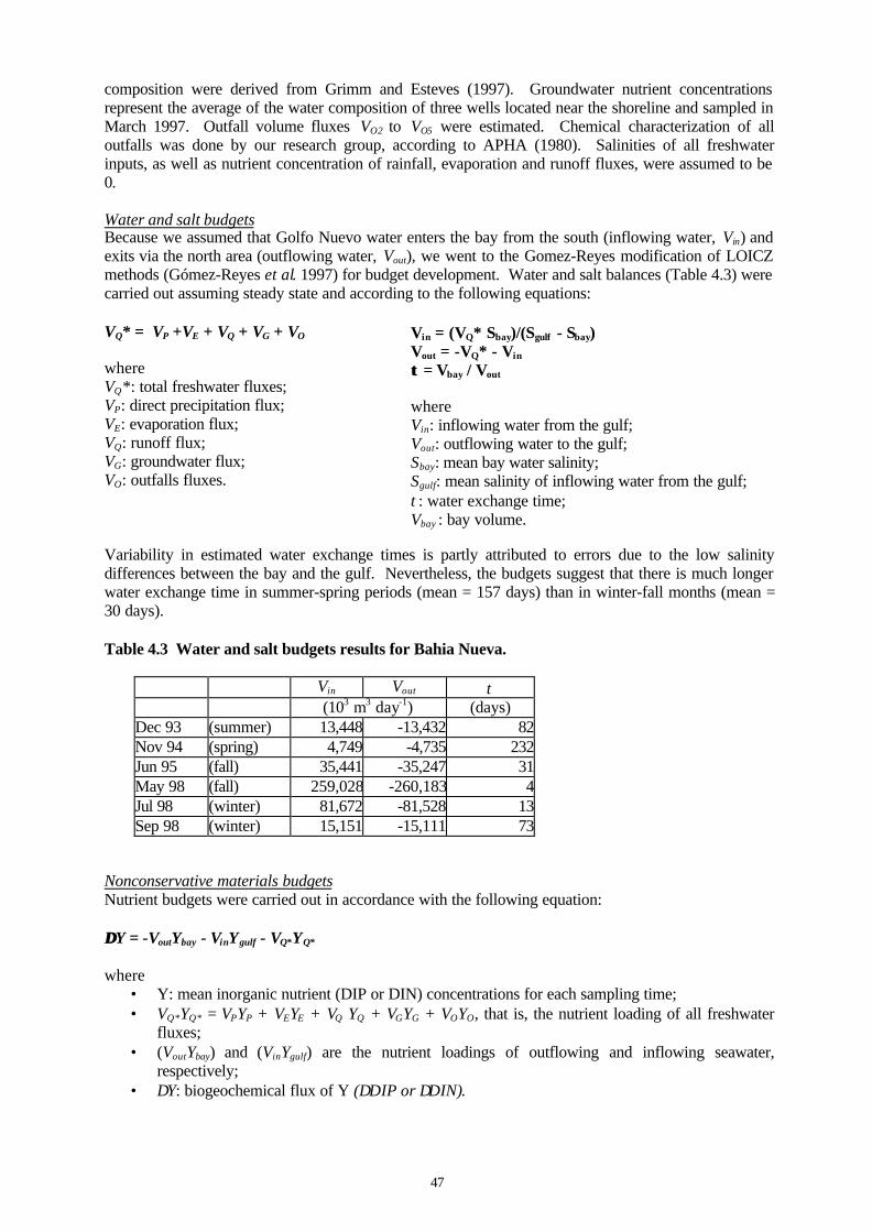
47

composition were derived from Grimm and Esteves (1997). Groundwater nutrient concentrationsrepresent the average of the water composition of three wells located near the shoreline and sampled inMarch 1997. Outfall volume fluxes VO2 to VO5 were estimated. Chemical characterization of alloutfalls was done by our research group, according to APHA (1980). Salinities of all freshwaterinputs, as well as nutrient concentration of rainfall, evaporation and runoff fluxes, were assumed to be0.

Water and salt budgetsBecause we assumed that Golfo Nuevo water enters the bay from the south (inflowing water, Vin) andexits via the north area (outflowing water, Vout), we went to the Gomez-Reyes modification of LOICZmethods (Gómez-Reyes et al. 1997) for budget development. Water and salt balances (Table 4.3) werecarried out assuming steady state and according to the following equations:

VQ* = VP +VE + VQ + VG + VO

whereVQ*: total freshwater fluxes;VP: direct precipitation flux;VE: evaporation flux;VQ: runoff flux;VG: groundwater flux;VO: outfalls fluxes.

Vin = (VQ* Sbay)/(Sgulf - Sbay)Vout = -VQ* - Vin

ττ = Vbay / Vout

whereVin: inflowing water from the gulf;Vout: outflowing water to the gulf;Sbay: mean bay water salinity;Sgulf: mean salinity of inflowing water from the gulf;τ: water exchange time;Vbay : bay volume.

Variability in estimated water exchange times is partly attributed to errors due to the low salinitydifferences between the bay and the gulf. Nevertheless, the budgets suggest that there is much longerwater exchange time in summer-spring periods (mean = 157 days) than in winter-fall months (mean =30 days).

Table 4.3 Water and salt budgets results for Bahia Nueva.

Vin Vout τ(103 m3 day-1) (days)

Dec 93 (summer) 13,448 -13,432 82Nov 94 (spring) 4,749 -4,735 232Jun 95 (fall) 35,441 -35,247 31May 98 (fall) 259,028 -260,183 4Jul 98 (winter) 81,672 -81,528 13Sep 98 (winter) 15,151 -15,111 73

Nonconservative materials budgetsNutrient budgets were carried out in accordance with the following equation:

∆∆Y = -VoutYbay - VinYgulf - VQ*YQ*

where• Y: mean inorganic nutrient (DIP or DIN) concentrations for each sampling time;• VQ*YQ* = VPYP + VEYE + VQ YQ + VGYG + VOYO, that is, the nutrient loading of all freshwater

fluxes;• (VoutYbay) and (VinYgulf) are the nutrient loadings of outflowing and inflowing seawater,

respectively;• ∆Y: biogeochemical flux of Y (∆DIP or ∆DIN).

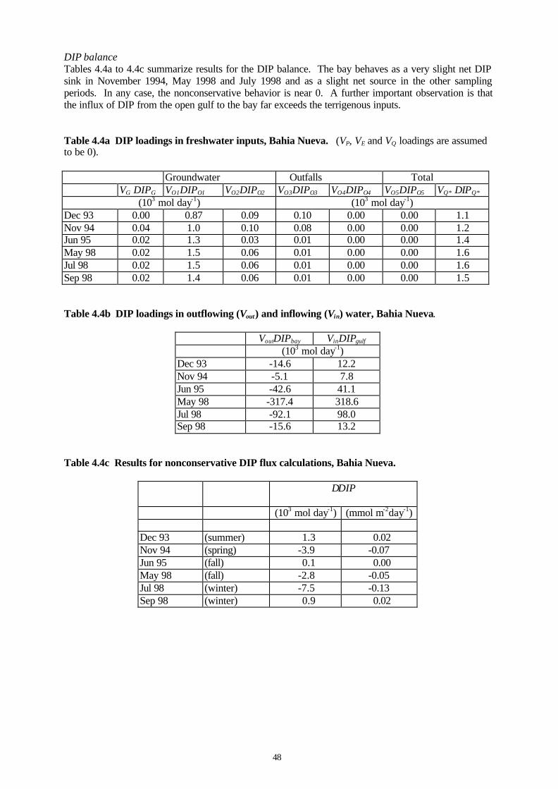
48

DIP balanceTables 4.4a to 4.4c summarize results for the DIP balance. The bay behaves as a very slight net DIPsink in November 1994, May 1998 and July 1998 and as a slight net source in the other samplingperiods. In any case, the nonconservative behavior is near 0. A further important observation is thatthe influx of DIP from the open gulf to the bay far exceeds the terrigenous inputs.

Table 4.4a DIP loadings in freshwater inputs, Bahia Nueva. (VP, VE and VQ loadings are assumedto be 0).

Groundwater Outfalls TotalVG DIPG VO1DIPO1 VO2DIPO2 VO3DIPO3 VO4DIPO4 VO5DIPO5 VQ* DIPQ*

(103 mol day-1) (103 mol day-1)Dec 93 0.00 0.87 0.09 0.10 0.00 0.00 1.1Nov 94 0.04 1.0 0.10 0.08 0.00 0.00 1.2Jun 95 0.02 1.3 0.03 0.01 0.00 0.00 1.4May 98 0.02 1.5 0.06 0.01 0.00 0.00 1.6Jul 98 0.02 1.5 0.06 0.01 0.00 0.00 1.6Sep 98 0.02 1.4 0.06 0.01 0.00 0.00 1.5

Table 4.4b DIP loadings in outflowing (Vout) and inflowing (Vin) water, Bahia Nueva.

VoutDIPbay VinDIPgulf

(103 mol day-1)Dec 93 -14.6 12.2Nov 94 -5.1 7.8Jun 95 -42.6 41.1May 98 -317.4 318.6Jul 98 -92.1 98.0Sep 98 -15.6 13.2

Table 4.4c Results for nonconservative DIP flux calculations, Bahia Nueva.

∆DIP

(103 mol day-1) (mmol m-2day-1)

Dec 93 (summer) 1.3 0.02Nov 94 (spring) -3.9 -0.07Jun 95 (fall) 0.1 0.00May 98 (fall) -2.8 -0.05Jul 98 (winter) -7.5 -0.13Sep 98 (winter) 0.9 0.02

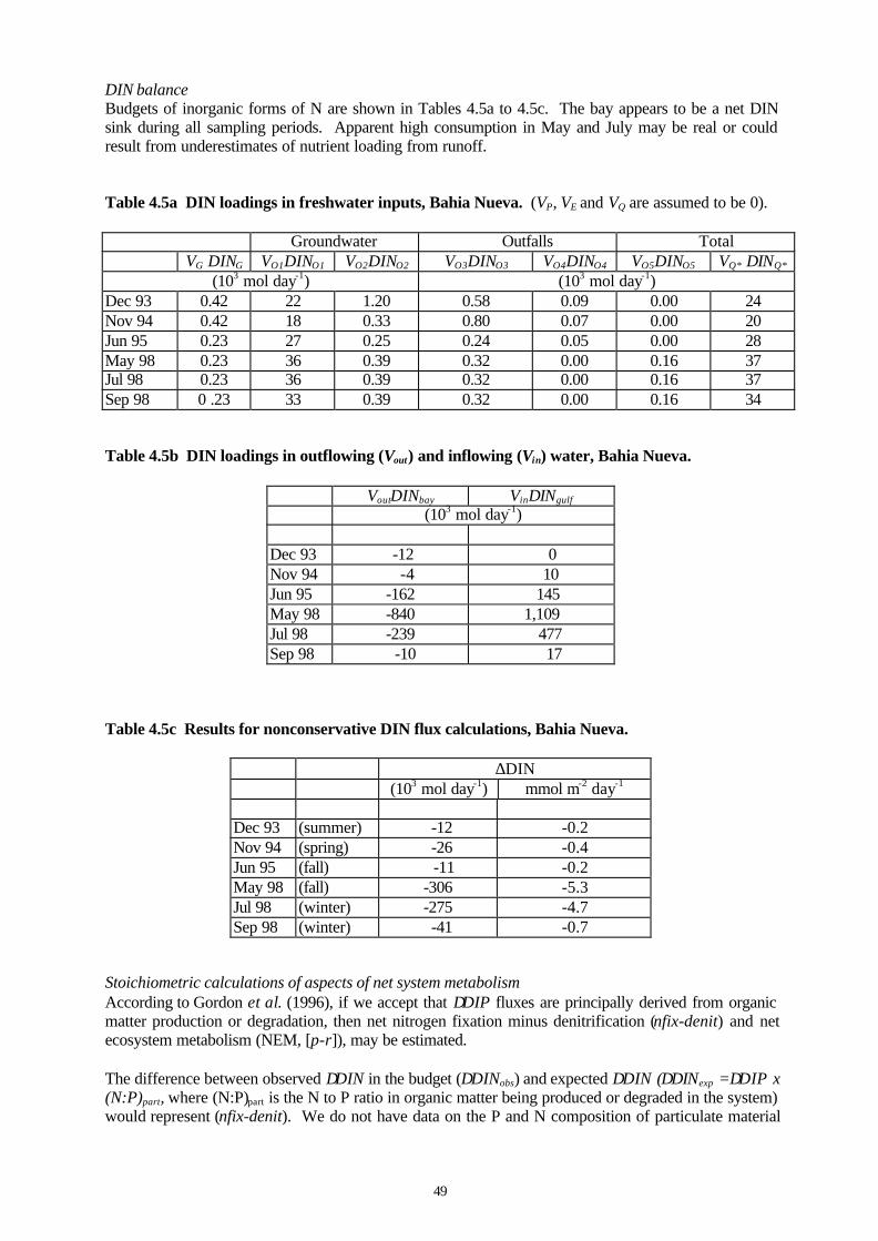
49

DIN balanceBudgets of inorganic forms of N are shown in Tables 4.5a to 4.5c. The bay appears to be a net DINsink during all sampling periods. Apparent high consumption in May and July may be real or couldresult from underestimates of nutrient loading from runoff.

Table 4.5a DIN loadings in freshwater inputs, Bahia Nueva. (VP, VE and VQ are assumed to be 0).

Groundwater Outfalls TotalVG DING VO1DINO1 VO2DINO2 VO3DINO3 VO4DINO4 VO5DINO5 VQ* DINQ*

(103 mol day-1) (103 mol day-1)Dec 93 0.42 22 1.20 0.58 0.09 0.00 24Nov 94 0.42 18 0.33 0.80 0.07 0.00 20Jun 95 0.23 27 0.25 0.24 0.05 0.00 28May 98 0.23 36 0.39 0.32 0.00 0.16 37Jul 98 0.23 36 0.39 0.32 0.00 0.16 37Sep 98 0 .23 33 0.39 0.32 0.00 0.16 34

Table 4.5b DIN loadings in outflowing (Vout) and inflowing (Vin) water, Bahia Nueva.

VoutDINbay VinDINgulf

(103 mol day-1)

Dec 93 -12 0Nov 94 -4 10Jun 95 -162 145May 98 -840 1,109Jul 98 -239 477Sep 98 -10 17

Table 4.5c Results for nonconservative DIN flux calculations, Bahia Nueva.

∆DIN(103 mol day-1) mmol m-2 day-1

Dec 93 (summer) -12 -0.2Nov 94 (spring) -26 -0.4Jun 95 (fall) -11 -0.2May 98 (fall) -306 -5.3Jul 98 (winter) -275 -4.7Sep 98 (winter) -41 -0.7

Stoichiometric calculations of aspects of net system metabolismAccording to Gordon et al. (1996), if we accept that ∆DIP fluxes are principally derived from organicmatter production or degradation, then net nitrogen fixation minus denitrification (nfix-denit) and netecosystem metabolism (NEM, [p-r]), may be estimated.

The difference between observed ∆DIN in the budget (∆DINobs) and expected ∆DIN (∆DINexp =∆DIP x(N:P)part, where (N:P)part is the N to P ratio in organic matter being produced or degraded in the system)would represent (nfix-denit). We do not have data on the P and N composition of particulate material

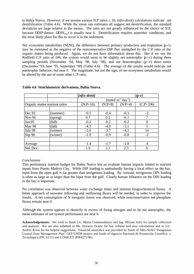
50

in Bahía Nueva. However, if we assume various N:P ratios ≤ 16, (nfix-denit) calculations indicate netdenitrification (Table 4.6). While the mean rate estimates all suggest net denitrification, the standarddeviations are large relative to the means. The rates are not greatly influenced by the choice of N:P,because ∆DIP (hence, ∆DINexp) is usually near 0. Denitrification requires anaerobic conditions, andthe most likely place for this to occur is in the sediments.

Net ecosystem metabolism (NEM), the difference between primary production and respiration (p-r),may be estimated as the negative of the nonconservative DIP flux multiplied by the C:P ratio of theorganic matter being produced. Again, we do not have information about this. But if we use theRedfield C:P ratio of 106, the system would seem to be slightly net autotrophic (p>r) during threesampling periods (November ′94, May ′98, July ′98), and net heterotrophic (p<r) three times(December ′93, June ′95, September ′98) (Table 4.6). The average of the results would indicate netautotrophic behavior, but near 0. The magnitude, but not the sign, of net ecosystem metabolism wouldbe altered by the use of some other C:P ratio.

Table 4.6 Stoichiometric derivations, Bahia Nueva.

(nfix-denit) (p-r)(mmol m-2 day-1)

Organic matter nutrient ratios (N:P=16) (N:P=8) (N:P=4) (C:P=106)

Dec 93 (summer) -0.5 -0.4 -0.3 -2Nov 94 (spring) 0.7 0.2 -0.1 7Jun 95 (fall) -0.2 -0.2 -0.2 0May 98 (fall) -4.5 -4.9 -5.1 5July 98 (winter) -2.6 -3.7 -4.2 14Sep 98 (winter) -1.0 -0.9 -0.8 -2

Average -1.4 -1.7 -1.8 4Std. Dev. 1.9 2.1 2.3 6

ConclusionsThis preliminary nutrient budget for Bahía Nueva lets us evaluate human impacts related to nutrientinputs from Puerto Madryn City. While DIP loading is undoubtedly having a local effect on the bay,input from the open gulf is far greater than terrigenous loading. By contrast, terrigenous DIN loadingis often as large as or larger than the input from the gulf. Clearly human influence on the DIN loadingto the bay is important.

No correlation was observed between water exchange times and nutrient biogeochemical fluxes. Abetter approach of seawater inflowing and outflowing fluxes will be needed, in order to improve theresults. A net consumption of N inorganic forms was observed, while nonconservative net phosphatefluxes remain near 0.

Although the system appears to denitrify in excess of fixing nitrogen and to be net autotrophic, themean estimates of net system performance are near 0.

Acknowledgements: We wish to thank Lic. Marta Commendatore and Ing. Miriam Solís for sample collectionand analysis. We are also indebted to Mr. Horacio Ocariz for bay volume and area calculations and to Lic.Andrés Rivas for his helpful suggestions. Financial assistance was provided by funds of ARG/92/63 "PatagonianCoastal Zone Management Plan" GEF/UNDP project and funds of Agencia Nacional de Promoción Científica yTecnológica (PIC 0111) and CONICET (PIP4271/96).

51

5. ECUADOR ESTUARINE SYSTEMS

5.1 Gulf of Guayaquil

Isabel Tutivén U.

Study areaGuayaquil Gulf, located between 2.0°-3.5° S, 79.5°-81.0°W, is the largest estuary of the Pacific coastof South America (Figure 5.1). Its waters are very productive and are fished by Ecuador and by othernations (Stevenson 1981). Plankton biomass is dominated by coccolithophores and diatoms with highplankton biomass. During the period studied by PMRC (1989), the net productivity in surface waterswas from 800 to 1000 mg C m-3 day-1 during the wet season, measured at one station.

The gulf has a surface area of 5,000 km2 and a drainage area of 51,000 km2 (Epler and Olsen 1993).The system can be divided into an outer estuary from Puna Island (located inside of the estuary at80.25°-81.0° W), and an inner estuary that extends upstream 75 km from Puna Island. It narrows to theGuayas River channel (Stevenson 1981). The maximum depth of the gulf decreases from 180 to 18 m(Figure 5.1).

Guayaquil Gulf

4.00°S

3.30°S

3.00°S

2.30°S

80.00°W80.30°W81.00°W

D A

B

0 20 Kilometers

QuayaquilGulf

The tidal regime is semi-diurnal and can range up to 5 m (Stevenson 1981); it decreases in the outerestuary. Tidal influence extends upstream to about 2.3°S. Salinity is >0 psu at the interior estuary indry season between August and November and 0 psu in the wet season (Tutivén 1993).

The Ecuadorian coast is in a transitional zone where two climatic systems meet, one from the NorthPacific and the other from the South Pacific. The boundary is the Inter-tropical Convergence Zone(ICZ). This boundary fluctuates, establishing the seasonal variations found in Ecuador. Because ofseasonal variability, waters from the north enter the Gulf during the wet season, and waters from thesouth enter during the dry season.

Figure 5.1 Location and map of Guayaquil Gulf, Ecuador.

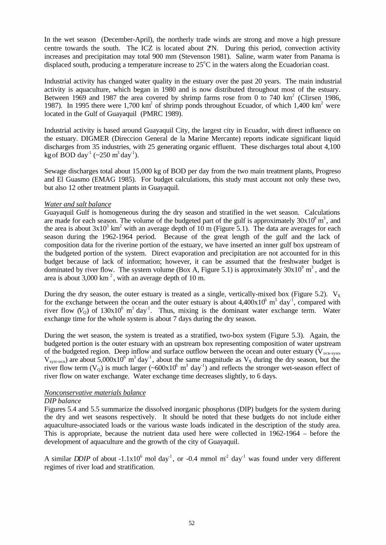
52

In the wet season (December-April), the northerly trade winds are strong and move a high pressurecentre towards the south. The ICZ is located about 2°N. During this period, convection activityincreases and precipitation may total 900 mm (Stevenson 1981). Saline, warm water from Panama isdisplaced south, producing a temperature increase to 25oC in the waters along the Ecuadorian coast.

Industrial activity has changed water quality in the estuary over the past 20 years. The main industrialactivity is aquaculture, which began in 1980 and is now distributed throughout most of the estuary.Between 1969 and 1987 the area covered by shrimp farms rose from 0 to 740 km2 (Clirsen 1986,1987). In 1995 there were 1,700 km2 of shrimp ponds throughout Ecuador, of which 1,400 km2 werelocated in the Gulf of Guayaquil (PMRC 1989).

Industrial activity is based around Guayaquil City, the largest city in Ecuador, with direct influence onthe estuary. DIGMER (Direccion General de la Marine Mercante) reports indicate significant liquiddischarges from 35 industries, with 25 generating organic effluent. These discharges total about 4,100kg of BOD day-1 (~250 m3 day-1).

Sewage discharges total about 15,000 kg of BOD per day from the two main treatment plants, Progresoand El Guasmo (EMAG 1985). For budget calculations, this study must account not only these two,but also 12 other treatment plants in Guayaquil.

Water and salt balanceGuayaquil Gulf is homogeneous during the dry season and stratified in the wet season. Calculationsare made for each season. The volume of the budgeted part of the gulf is approximately 30x109 m3 , andthe area is about 3x103 km2 with an average depth of 10 m (Figure 5.1). The data are averages for eachseason during the 1962-1964 period. Because of the great length of the gulf and the lack ofcomposition data for the riverine portion of the estuary, we have inserted an inner gulf box upstream ofthe budgeted portion of the system. Direct evaporation and precipitation are not accounted for in thisbudget because of lack of information; however, it can be assumed that the freshwater budget isdominated by river flow. The system volume (Box A, Figure 5.1) is approximately 30x109 m3 , and thearea is about 3,000 km 2 , with an average depth of 10 m.

During the dry season, the outer estuary is treated as a single, vertically-mixed box (Figure 5.2). VX

for the exchange between the ocean and the outer estuary is about 4,400x106 m3 day-1, compared withriver flow (VQ) of 130x106 m3 day-1. Thus, mixing is the dominant water exchange term. Waterexchange time for the whole system is about 7 days during the dry season.

During the wet season, the system is treated as a stratified, two-box system (Figure 5.3). Again, thebudgeted portion is the outer estuary with an upstream box representing composition of water upstreamof the budgeted region. Deep inflow and surface outflow between the ocean and outer estuary (Vocn-syst,Vsyst-ocn) are about 5,000x106 m3 day-1 , about the same magnitude as VX during the dry season, but theriver flow term (VQ) is much larger (~600x106 m3 day-1) and reflects the stronger wet-season effect ofriver flow on water exchange. Water exchange time decreases slightly, to 6 days.

Nonconservative materials balanceDIP balanceFigures 5.4 and 5.5 summarize the dissolved inorganic phosphorus (DIP) budgets for the system duringthe dry and wet seasons respectively. It should be noted that these budgets do not include eitheraquaculture-associated loads or the various waste loads indicated in the description of the study area.This is appropriate, because the nutrient data used here were collected in 1962-1964 – before thedevelopment of aquaculture and the growth of the city of Guayaquil.

A similar ∆DIP of about -1.1x106 mol day-1 , or -0.4 mmol m-2 day-1 was found under very differentregimes of river load and stratification.

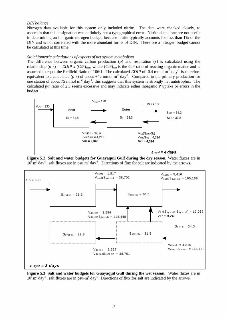
53

DIN balanceNitrogen data available for this system only included nitrite. The data were checked closely, toascertain that this designation was definitely not a typographical error. Nitrite data alone are not usefulin determining an inorganic nitrogen budget, because nitrite typically accounts for less than 1% of theDIN and is not correlated with the more abundant forms of DIN. Therefore a nitrogen budget cannotbe calculated at this time.

Stoichiometric calculations of aspects of net system metabolismThe difference between organic carbon production (p) and respiration (r) is calculated using therelationship (p-r) = -∆DIP x (C:P)part, where (C:P)part is the C:P ratio of reacting organic matter and isassumed to equal the Redfield Ratio of 106:1. The calculated ∆DIP of -0.4 mmol m-2 day-1 is thereforeequivalent to a calculated (p-r) of about +42 mmol m-2 day-1. Compared to the primary production forone station of about 75 mmol m-2 day-1, this suggests that this system is strongly net autotrophic. Thecalculated p/r ratio of 2.3 seems excessive and may indicate either inorganic P uptake or errors in thebudget.

Figure 5.2 Salt and water budgets for Guayaquil Gulf during the dry season. Water fluxes are in106 m3 day-1; salt fluxes are in psu m3 day-1. Directions of flux for salt are indicated by the arrows.

Figure 5.3 Salt and water budgets for Guayaquil Gulf during the wet season. Water fluxes are in106 m3 day-1; salt fluxes are in psu-m3 day-1. Directions of flux for salt are indicated by the arrows.

VQ1 = 130VR2 = 130

Socn = 34.3

SR2 = 33.8

VX2(Socn-S2) = -VR2SR2 = 4,394 VX2 = 4,394

VX1(S2 - S1) = -VR1SR1 = 4,212 VX1 = 2,340

VR1 = 130

τ τ syst = 4 days

Inner

S1 = 31.5

Outer

S2 = 33.3

V surf2 = 5,416 V surf2Ssyst-s2 = 165,189

VZ 2(S syst-d2-Ssyst-s2) = 12,039 VZ2 = 9,261

Vdeep2' = 3,599 Vdeep2'Ssyst-d2 = 114,448

Vdeep2 = 4,816 Vdeep2Socn-d = 165,189

Socn-d = 34.3

Ssyst-s2 = 30.5

S syst-d2 = 31.8

V surf1 = 1,817 V surf1Ssyst-s1 = 38,702

Vdeep1 = 1,217 Vdeep1Ssyst-d2 = 38,701

S Q = 600

Ssyst-s1 = 21.3

Ssyst-d1 = 22.8

τ τ syst = 3 days

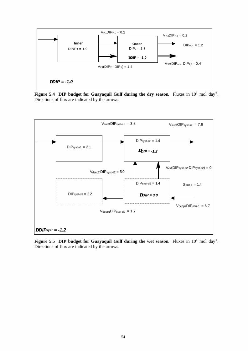
54

Figure 5.4 DIP budget for Guayaquil Gulf during the dry season. Fluxes in 106 mol day-1.Directions of flux are indicated by the arrows.

Figure 5.5 DIP budget for Guayaquil Gulf during the wet season. Fluxes in 106 mol day-1.Directions of flux are indicated by the arrows.

Outer DIP2 = 1.3

∆∆DIP = -1.0

VR2DIPR2 = 0.2

DIPocn = 1.2

VX2(DIPocn-DIP2) = 0.4

Inner

DINP1 = 1.9

VX1(DIP2 - DIP1) = 1.4

VR1DIPR1 = 0.2

∆∆DIP = -1.0

Vsurf2DIPsyst-s2 = 7.6

VZ2(DIPsyst-d2-DIPsyst-s2) = 0Vdeep2'DIPsyst-d2 = 5.0

Vdeep2DIPocn-d = 6.7

Socn-d = 1.4

DIPsyst-s2 = 1.4

∆∆DIP = -1.2

DIPsyst-d2 = 1.4

∆∆DIP = 0.0

Vsurf1DIPsyst-s1 = 3.8

Vdeep1DIPsyst-d2 = 1.7

DIPsyst-s1 = 2.1

DIPsyst-d1 = 2.2


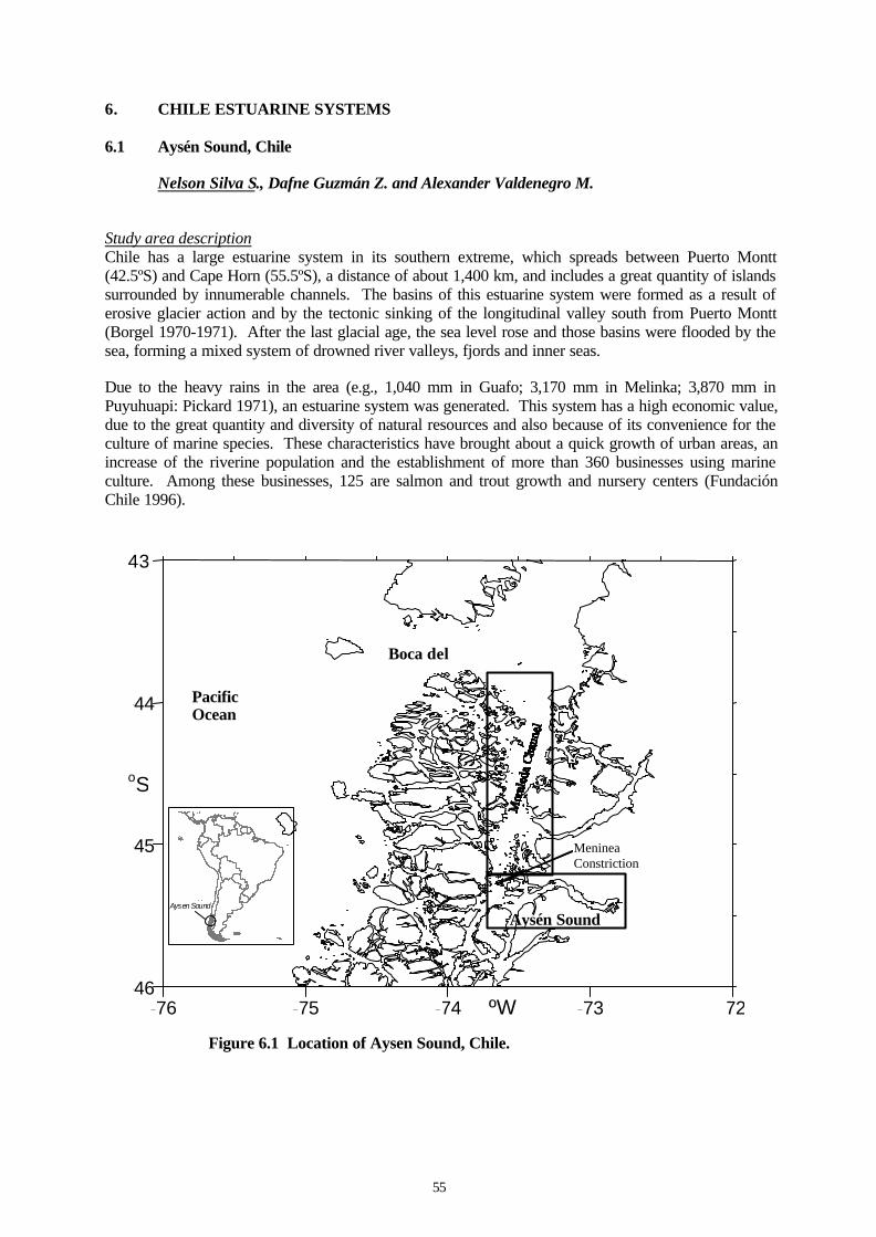
55

6. CHILE ESTUARINE SYSTEMS

6.1 Aysén Sound, Chile

Nelson Silva S., Dafne Guzmán Z. and Alexander Valdenegro M.

Study area descriptionChile has a large estuarine system in its southern extreme, which spreads between Puerto Montt(42.5ºS) and Cape Horn (55.5ºS), a distance of about 1,400 km, and includes a great quantity of islandssurrounded by innumerable channels. The basins of this estuarine system were formed as a result oferosive glacier action and by the tectonic sinking of the longitudinal valley south from Puerto Montt(Borgel 1970-1971). After the last glacial age, the sea level rose and those basins were flooded by thesea, forming a mixed system of drowned river valleys, fjords and inner seas.

Due to the heavy rains in the area (e.g., 1,040 mm in Guafo; 3,170 mm in Melinka; 3,870 mm inPuyuhuapi: Pickard 1971), an estuarine system was generated. This system has a high economic value,due to the great quantity and diversity of natural resources and also because of its convenience for theculture of marine species. These characteristics have brought about a quick growth of urban areas, anincrease of the riverine population and the establishment of more than 360 businesses using marineculture. Among these businesses, 125 are salmon and trout growth and nursery centers (FundaciónChile 1996).

-76 -75 -74 -73 -72-46

-45

-44

43

Boca delGuafo

Aysén Sound

MenineaConstriction

PacificOcean

ºW

oS

Figure 6.1 Location of Aysen Sound, Chile.

Aysen Sound

56

Hydrographic AspectsAysén Sound is a fjord which is located between 45.3°-45.5°S, 72.8º-73.8ºW, with a length of about 73km, an average depth of 142 m and an area of about 470 km2. Its mouth is connected to the southernextreme of the Moraleda Channel which is in turn connected to the sea at its northern extreme throughthe “Boca del Guafo” (Figure 6.1).

The Aysén River flows into the head of this fjord, and it has as principal discharges the Mañiguales (15million m3 day-1), the Simpson (9 million m3 day-1) and the Claro (500 thousand m3 day-1) rivers. Inaddition, the Cuervo (9 million m3 day-1) and Lagunillas (4 million m3 day-1) rivers flow directly intothe fjord (Ministerio de Obras Públicas 1997). There are other rivers for which there are no flowrecords; but which seem to be relatively unimportant.

Due to the large freshwater contribution from rivers and rain, Aysén Sound is characterized by a two-layer structure, separated by a strong halocline. The upper layer, which is about 25 m thick, hassalinities between 0 psu at the head and 29 psu at the mouth. The lower layer is more homogeneous,with salinities between 30 and 31 psu (Figure 6.2) (Sievers and Prado 1994; Silva et al. 1995, 1997).The upper layers are well-oxygenated throughout the sound and have concentrations from 5 to 7 ml l-1.However, the lower layers have concentrations about 5 ml l-1 in the first third of the sound, but then itrapidly decreases towards the head to values lower than 2.5 ml l-1 near the bottom (Silva et al. 1995,1997). This situation is also seen in the pH measurements in the area, which are 7.75 at the mouth and7.35 at the head (Silva et al. 1997).

Nitrate (DIN) and phosphate (DIP) also show a two-layer structure, with lower values at the surface,due to the contribution of low-nutrient rivers (Silva et al. 1990a, 1990b) and biological uptake. Theupper layer has concentrations of 0-1.2 µM of phosphate and 0-12 µM of nitrate. The lower layer ismore homogeneous, with concentrations of 1.4-1.8 µM of phosphate and 1.2-12 µM nitrate, increasingfrom the mouth to the head (Silva et al. 1997). The average N:P Redfield ratios for the sound waters,obtained by linear regression, were 10.6:1 with a correlation coefficient of 0.971 (Calvete 1997).

The decrease of dissolved oxygen and pH and the increase of dissolved nutrients towards the head ofthe fjord indicate a strong remineralization of organic material at the head of the fjord. The abovewould be due principally to the nutrient regeneration from marine organic matter produced in the soundand terrestrial organic matter brought by the rivers. A probable sluggish circulation in this upper partof the sound will contribute to the permanence of high values of DIN and DIP. Chemicalmeasurements in sound sediments show high concentrations of organic matter (8-10%), organic carbon(1.5-4%) and Kjeldahl nitrogen (0.1-0.3%) (Silva et al. 1998), which are characteristic of the highlyproductive areas.

General circulationNear the southern extreme of the Moraleda channel, off Meninea island (45.27º S; 73.63º W), there is ashallow sill (60 m deep), which makes the southern part of the Moraleda channel and Aysén Soundform a deep basin partially isolated from the open ocean. This “Meninea constriction” constrains thecirculation in the levels below the sill (60-300 m) and results in different oceanographic characteristicsin the two basins. The southern basin is warmer, less saline and more oxygenated than the northernone, which is connected to the open ocean through the Guafo mouth.

The former situation, where the isolated basin is more oxygenated than the basin with free exchange tothe open ocean, could be explained on the basis of an estuarine circulation mechanism and the presencein the channels of low oxygen deep water from Equatorial Subsurface origin (Silva et al. 1995). Thewater from the 25 to 60 m depths has a small net flow towards the south that allows the northern basinwater to pass into the southern basin, where it sinks into deeper levels because of its higher densitythan the interior water. Thus 25 to 60 m water fills most of the deep part of the southern basin,carrying its characteristics and producing the situation described above. In order to maintain thevolume balance, the less saline upper layer water of the southern basin has a net flow to the north,flowing out towards the adjacent oceanic area.

57

A net current of 16 cm sec-1 towards the ocean for the surface layer, and a net current of 2 cm sec-1 forthe subsurface layer, have been shown as a result of two-month current meter measurements in theMeninea area (Salinas and Hormazábal 1996).

Water and salt budgetsBy means of the employment of a two-layer box model and based on the methodology proposed byLOICZ, a water and salt budget for Aysén Sound was prepared. To do that, the following assumptionswere made:

- VG = 0 and SG = 0 (groundwater), since it was not possible to estimate them. In any case, the termsseem likely to be small compared with river flow and rainfall.

- V0 = 0 and S0 = 0 (riverine fresh water). These terms were considered irrelevant, since the greatersources of freshwater are the rivers and the rain.

- VE = 0 (evaporation), since it was considered as minor term in the estuarine system compared withhigh precipitation volumes (≈2 m year-1) and relatively low mean annual air temperature (≈10oC)of the area.

- VQ (River flow) was obtained based on historical records of the Mañiguales, Simpson, Claro,Lagunillas and Cuervo rivers, which provide the estuarine system with fresh water. Since monthlyrecords were available, the records were divided into two seasonal periods (summer and winter).These values were increased by 30%, to correct them for freshwater input provided by rivers andcoastal runoff for which there are no records.

- SQ (river salinity) was assumed to be 0.1 psu, as has been reported in other studies.

- VP (precipitation) was obtained based on historical records from Puerto Aysén (DirecciónMeteorológica de Chile 1983-1996). Monthly records were compiled into two seasonal periods(summer and winter).

- Due to the presence of a halocline centered around 25 m depth, the box model was considered as atwo-layer one, with the first layer in the upper 25 m and the second below 25 m.

- Due to the presence of the Meninea constriction (which behaves as a physical barrier to watermovement), the 25-80 m stratum was considered as the deep layer of the oceanic box. Meanwhilein the estuarine system, the deep layer was considered to cover the strata from 25 m to the bottom.

- The Meninea constriction was considered as the limit of the estuarine system, since it represents aphysical barrier between the oceanic and the estuarine system.

Based on the previously stated considerations, and data taken by Cimar Fiordo 1 (winter 1995), CimarFiordo 4-1, (winter 1998) and Cimar Fiordo 4-2, (summer 1999) cruises, a water and salt budget forAysén Sound was prepared (Tables 6.1 and 6.2; Figures 6.3, 6.6, 6.9).

Even though the area is very rainy ( precipitation ≈2 m yr-1 ), it shows some degree of seasonality inprecipitation and river discharge (Table 6.1). Therefore, the available data were analyzed in two parts:a southern fall-winter (April to October) period and southern spring-summer (November to March)period. Figures 6.3 and 6.6 summarize the water and salt budgets for two cruises performed in latewinter (October 1995 and 1998), and Figure 6.9 summarizes the water and salt budgets for a cruiseperformed in late summer (March 1999). The river flow and precipitation used in the budgets (Table6.2) correspond to seasonal averages based on monthly historical data taken during several years(Dirección Meteorológica de Chile 1983-1996).

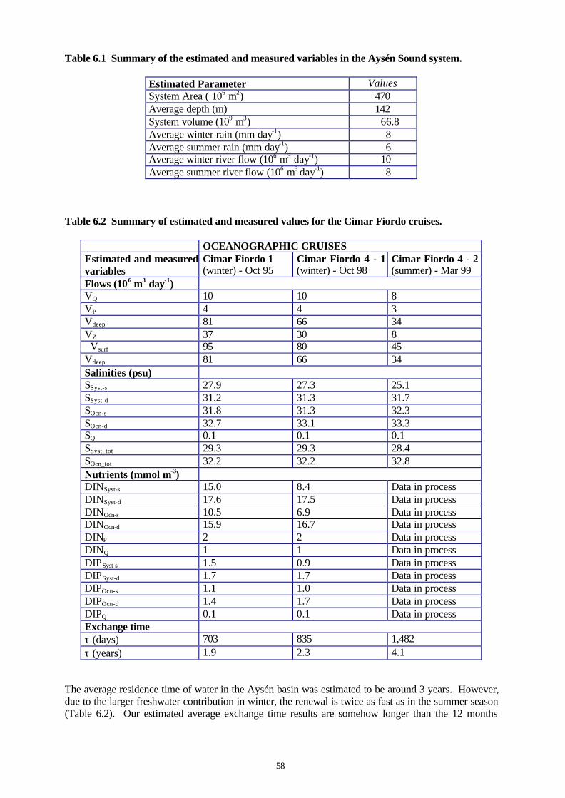
58

Table 6.1 Summary of the estimated and measured variables in the Aysén Sound system.

Estimated Parameter ValuesSystem Area ( 106 m2) 470Average depth (m) 142System volume (109 m3) 66.8Average winter rain (mm day-1) 8Average summer rain (mm day-1) 6Average winter river flow (106 m3 day-1) 10Average summer river flow (106 m3 day-1) 8

Table 6.2 Summary of estimated and measured values for the Cimar Fiordo cruises.

OCEANOGRAPHIC CRUISESEstimated and measuredvariables

Cimar Fiordo 1(winter) - Oct 95

Cimar Fiordo 4 - 1(winter) - Oct 98

Cimar Fiordo 4 - 2(summer) - Mar 99

Flows (106 m3 day-1)VQ 10 10 8VP 4 4 3Vdeep 81 66 34VZ 37 30 8 Vsurf 95 80 45Vdeep 81 66 34Salinities (psu)SSyst-s 27.9 27.3 25.1SSyst-d 31.2 31.3 31.7SOcn-s 31.8 31.3 32.3SOcn-d 32.7 33.1 33.3SQ 0.1 0.1 0.1SSyst_tot 29.3 29.3 28.4SOcn_tot 32.2 32.2 32.8Nutrients (mmol m-3)DINSyst-s 15.0 8.4 Data in processDINSyst-d 17.6 17.5 Data in processDINOcn-s 10.5 6.9 Data in processDINOcn-d 15.9 16.7 Data in processDINP 2 2 Data in processDINQ 1 1 Data in processDIPSyst-s 1.5 0.9 Data in processDIPSyst-d 1.7 1.7 Data in processDIPOcn-s 1.1 1.0 Data in processDIPOcn-d 1.4 1.7 Data in processDIPQ 0.1 0.1 Data in processExchange timeτ (days) 703 835 1,482τ (years) 1.9 2.3 4.1

The average residence time of water in the Aysén basin was estimated to be around 3 years. However,due to the larger freshwater contribution in winter, the renewal is twice as fast as in the summer season(Table 6.2). Our estimated average exchange time results are somehow longer than the 12 months

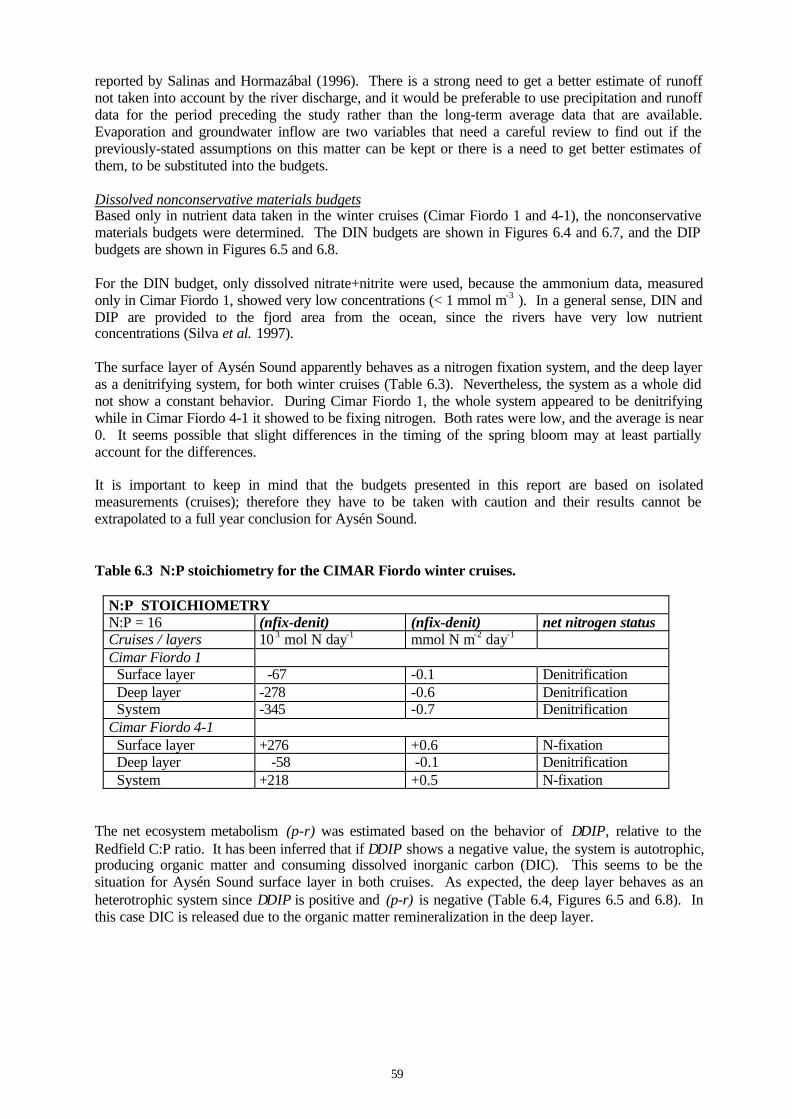
59

reported by Salinas and Hormazábal (1996). There is a strong need to get a better estimate of runoffnot taken into account by the river discharge, and it would be preferable to use precipitation and runoffdata for the period preceding the study rather than the long-term average data that are available.Evaporation and groundwater inflow are two variables that need a careful review to find out if thepreviously-stated assumptions on this matter can be kept or there is a need to get better estimates ofthem, to be substituted into the budgets.

Dissolved nonconservative materials budgetsBased only in nutrient data taken in the winter cruises (Cimar Fiordo 1 and 4-1), the nonconservativematerials budgets were determined. The DIN budgets are shown in Figures 6.4 and 6.7, and the DIPbudgets are shown in Figures 6.5 and 6.8.

For the DIN budget, only dissolved nitrate+nitrite were used, because the ammonium data, measuredonly in Cimar Fiordo 1, showed very low concentrations (< 1 mmol m-3 ). In a general sense, DIN andDIP are provided to the fjord area from the ocean, since the rivers have very low nutrientconcentrations (Silva et al. 1997).

The surface layer of Aysén Sound apparently behaves as a nitrogen fixation system, and the deep layeras a denitrifying system, for both winter cruises (Table 6.3). Nevertheless, the system as a whole didnot show a constant behavior. During Cimar Fiordo 1, the whole system appeared to be denitrifyingwhile in Cimar Fiordo 4-1 it showed to be fixing nitrogen. Both rates were low, and the average is near0. It seems possible that slight differences in the timing of the spring bloom may at least partiallyaccount for the differences.

It is important to keep in mind that the budgets presented in this report are based on isolatedmeasurements (cruises); therefore they have to be taken with caution and their results cannot beextrapolated to a full year conclusion for Aysén Sound.

Table 6.3 N:P stoichiometry for the CIMAR Fiordo winter cruises.

N:P STOICHIOMETRYN:P = 16 (nfix-denit) (nfix-denit) net nitrogen statusCruises / layers 10 3 mol N day-1 mmol N m-2 day-1

Cimar Fiordo 1 Surface layer -67 -0.1 Denitrification Deep layer -278 -0.6 Denitrification System -345 -0.7 DenitrificationCimar Fiordo 4-1 Surface layer +276 +0.6 N-fixation Deep layer -58 -0.1 Denitrification System +218 +0.5 N-fixation

The net ecosystem metabolism (p-r) was estimated based on the behavior of ∆DIP, relative to theRedfield C:P ratio. It has been inferred that if ∆DIP shows a negative value, the system is autotrophic,producing organic matter and consuming dissolved inorganic carbon (DIC). This seems to be thesituation for Aysén Sound surface layer in both cruises. As expected, the deep layer behaves as anheterotrophic system since ∆DIP is positive and (p-r) is negative (Table 6.4, Figures 6.5 and 6.8). Inthis case DIC is released due to the organic matter remineralization in the deep layer.

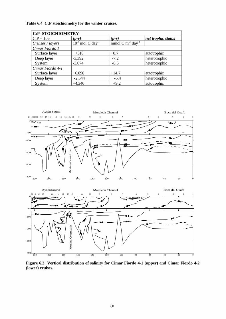
60

Table 6.4 C:P stoichiometry for the winter cruises.

C:P STOICHIOMETRYC:P = 106 (p-r) (p-r) net trophic statusCruises / layers 10 3 mol C day-1 mmol C m-2 day-1

Cimar Fiordo 1 Surface layer +318 +0.7 autotrophic Deep layer -3,392 -7.2 heterotrophic System -3,074 -6.5 heterotrophicCimar Fiordo 4-1 Surface layer +6,890 +14.7 autotrophic Deep layer -2,544 -5.4 heterotrophic System +4,346 +9.2 autotrophic

Boca del Guafo

-400

-300

-200

-100

-220 -200 -180 -160 -140 -120 -100 -80 -60 -40 -20 0

-50

0

1234578910111212a131415161717s18192021

Moraleda ChannelAysén Sound

< 20

-50

0> 8

123457891011121314151617181921

Boca del GuafoMoraleda ChannelAysén Sound

6

-220 -200 -180 -160 -140 -120 -100 -80 -60 -40 -20 0-400

-300

-200

-100

Men

inea

Con

stri

ctio

nM

enin

ea C

onst

rict

ion

Figure 6.2 Vertical distribution of salinity for Cimar Fiordo 4-1 (upper) and Cimar Fiordo 4-2(lower) cruises.

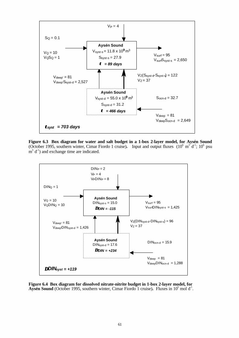
61

Figure 6.3 Box diagram for water and salt budget in a 1-box 2-layer model, for Aysén Sound(October 1995, southern winter, Cimar Fiordo 1 cruise). Input and output fluxes (106 m3 d-1; 106 psum3 d-1) and exchange time are indicated.

Figure 6.4 Box diagram for dissolved nitrate-nitrite budget in 1-box 2-layer model, forAysén Sound (October 1995, southern winter, Cimar Fiordo 1 cruise). Fluxes in 103 mol d-1.

VP = 4

Vsurf = 95 VsurfSsyst-s = 2,650

VZ(Ssyst-d-Ssyst-s) = 122 VZ = 37

Vdeep' = 81 Vdeep'Ssyst-d = 2,527

Vdeep = 81 VdeepSocn-d = 2,649

SQ = 0.1

Socn-d = 32.7

ττsyst = 703 days

Aysén Sound Vsyst-s = 11.8 x 10 m

Ssyst-s = 27.9

τ τ = 89 days

39

Aysén Sound Vsyst-d = 55.0 x 10 m

Ssyst-d = 31.2

τ τ = 466 days

39

VQ = 10 VQSQ = 1

VP = 4 VPDINP = 8

Vsurf = 95 VsurfDINsyst-s = 1,425

VZ(DINsyst-d-DINsyst-s) = 96 VZ = 37

Vdeep' = 81 Vdeep'DINsyst-d = 1,426

Vdeep = 81 VdeepDINocn-d = 1,288

DINQ = 1

DINocn-d = 15.9

∆∆DINsyst = +119

Aysén Sound DINsyst-s = 15.0

∆∆DIN = -115

VQ = 10 VQDINQ = 10

Aysén Sound DINsyst-d = 17.6

∆∆DIN = +234

DINP = 2

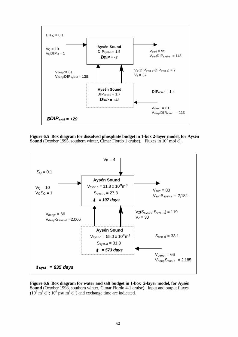
62

Figure 6.5 Box diagram for dissolved phosphate budget in 1-box 2-layer model, for AysénSound (October 1995, southern winter, Cimar Fiordo 1 cruise). Fluxes in 103 mol d-1.

Figure 6.6 Box diagram for water and salt budget in 1-box 2-layer model, for AysénSound (October 1998, southern winter, Cimar Fiordo 4-1 cruise). Input and output fluxes(106 m3 d-1; 106 psu m3 d-1) and exchange time are indicated.

Vsurf = 95 VsurfDIPsyst-s = 143

VZ(DIPsyst-d-DIPsyst-s) = 7 VZ = 37

Vdeep' = 81 Vdeep'DIPsyst-d = 138

Vdeep = 81 Vdeep DIPocn-d = 113

DIPQ = 0.1

DIPocn-d = 1.4

∆∆DIPsyst = +29

Aysén Sound DIPsyst-s = 1.5

∆∆DIP = -3

VQ = 10 VQDIPQ = 1

Aysén Sound DIPsyst-d = 1.7

∆∆DIP = +32

VP = 4



Vdeep' = 66 Vdeep'Ssyst-d =2,066


SQ = 0.1

Socn-d = 33.1

ττsyst = 835 days


Ssyst-s = 27.3

τ τ = 107 days

39

Aysén Sound Vsyst-d = 55.0 x 10 m

Ssyst-d = 31.3

τ τ = 573 days

39

VQ = 10 VQSQ = 1

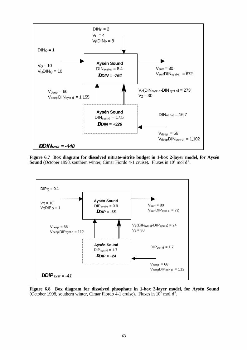
63

Figure 6.7 Box diagram for dissolved nitrate-nitrite budget in 1-box 2-layer model, for AysénSound (October 1998, southern winter, Cimar Fiordo 4-1 cruise). Fluxes in 103 mol d-1.

Figure 6.8 Box diagram for dissolved phosphate in 1-box 2-layer model, for Aysén Sound(October 1998, southern winter, Cimar Fiordo 4-1 cruise). Fluxes in 103 mol d-1.

Vsurf = 80 VsurfDIPsyst-s = 72

VZ(DIPsyst-d-DIPsyst-s) = 24 VZ = 30

Vdeep' = 66 Vdeep'DIPsyst-d = 112

Vdeep = 66 VdeepDIPocn-d = 112

DIPQ = 0.1

DIPocn-d = 1.7

∆∆DIPsyst = -41

Aysén Sound DIPsyst-s = 0.9

∆∆DIP = -65

VQ = 10 VQDIPQ = 1

Aysén Sound DIPsyst-d = 1.7

∆∆DIP = +24

VP = 4 VPDINP = 8

Vsurf = 80 VsurfDINsyst-s = 672

VZ(DIN syst-d-DIN syst-s) = 273 VZ = 30

Vdeep' = 66 Vdeep'DINsyst-d = 1,155

Vdeep = 66 VdeepDINocn-d = 1,102

DINQ = 1

DINocn-d = 16.7

∆∆DINsyst = -448

Aysén Sound DINsyst-s = 8.4

∆∆DIN = -764

VQ = 10 VQDINQ = 10

Aysén Sound DINsyst-d = 17.5

∆∆DIN = +326

DINP = 2

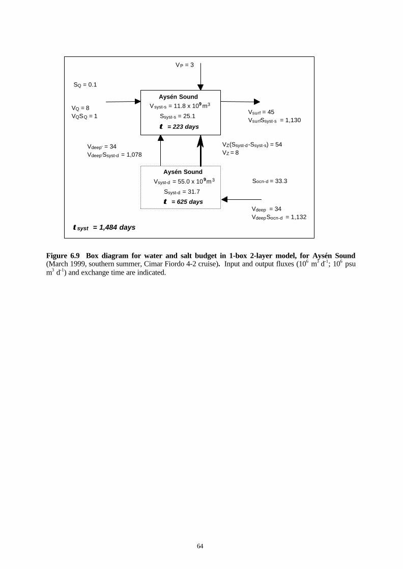
64

Figure 6.9 Box diagram for water and salt budget in 1-box 2-layer model, for Aysén Sound(March 1999, southern summer, Cimar Fiordo 4-2 cruise). Input and output fluxes (106 m3 d-1; 106 psum3 d-1) and exchange time are indicated.

VP = 3



Vdeep' = 34 Vdeep'Ssyst-d = 1,078


SQ = 0.1

Socn-d = 33.3

ττsyst = 1,484 days


Ssyst-s = 25.1

τ τ = 223 days

39

Aysén Sound

Vsyst-d = 55.0 x 10 m

Ssyst-d = 31.7

τ τ = 625 days

39

VQ = 8 VQSQ = 1

65

7. REFERENCES

ADEMA 1984 Levantamento da flora e caracterização dos bosques de mangue do estado de Sergipe.Technical report, ADEMA, Aracaju, 208 pages.

Alcântara, A.V., Rocha, C.E.F. and Santos, M.A. 1979 Caracterização hidrológica e biológica doestuário do Rio Sergipe. Technical report, ITPS/UFS/CNPq , Aracaju, 151 pages.

Alves, J.P.H. 1989 Características físico-químicas da água e comportamento dos nutrientes. Projetointegrado para a avaliação da potencialidade do estuário dos rios Piauí-Fundo-Real. Technicalreport, NEM/UFS , Vol. II, Aracaju, 74 pages.

Andrade, R.C.B., Souza, M.F.L. and Couto, E.C.G. 1998 Influência de efluentes têxteis e alimentíciossobre o metabolismo e propriedades físicas e químicas do Rio Piauitinga. Química Nova21(4):424-427.

André, D.L. 1990 Análise dos parâmetros hidroquímicos na ressurgência de Cabo Frio. MSc. Thesis.Universidade Federal Fluminense, Departamento de Geoquímica, Niterói.

APHA (eds) 1980 Standard methods for the examination of water and wastewater. 15th Ed., 1134pages.

Barbiéri, E.B. 1985 Condiçoes climáticas dominantes na porção oreintal da lagoa de Araruama (RJ) esuas implicações na diversidade do teor de salinidade. Caderno de Ciências da Terra 59:3-35.

Blanco, A.C. 1989 Balance de masa de los silicatos en la superficie del Río de la Plata y su área deinfluencia en el Mar Epicontinental uruguayo. Tesis para optar a la Licenciatura enOceanografía Biológica. Facultad de Humanides y Ciencias, Montevideo, Uruguay, 91 pages.

Borgel, R. 1970-1971 Geomorfología de las regiones australes de Chile. Revista Geológica de Chile21:35-140.

Brandini, F.P. 1985 Ecological studies in the Bay of Paranaguá I. Horizontal distribution and seasonaldynamics of the phytoplankton. Bol. Inst. Oceanogr., S. Paulo 33:139-147.

Calvete, C. 1997 Distribución de temperatura, salinidad, oxígeno disuelto, pH y nutrientesinorgánicos, en la zona de canales australes de Chile, entre Puerto Montt y Laguna San Rafaelen la primavera de 1995. Tesis de Titulación de Oceanógrafo, Escuela de Ciencias del Mar,Universidad católica de Valparaíso, 136 pages.

Campos, R.C., Queiroz, M.I., Lacerda, R.E.D. and Okuda, T. 1979 Conteúdo de fósforo total, carbonoe nitrogênio na forma orgânica, nos sedimentos da lagoa de Araruama. Instituto de Pesquisasda Marinha, Ministério da Marinha, Brazil 142, 7 pages.

Carmouze, J-P., D’Elia, C.S., Farias, B., Silva, S. and Azevedo, S. 1993 Ecological changes of ashallow Brazilian lagoon related to distrophic crisis. Verhandlungen Internationaler Vereinder Limnologie 251: 23-25.

Carmouze, J-P., D’Elia, C.S., Farias, B., Silva, S. and Azevedo, S. 1993 Ecological changes of ashallow Brazilian lagoon related to distrophic crisis. Verhandlungen Internationaler Vereinder Limnologie 251:23-25.

Carneiro, M.E. 1992 Ciclo anual do aporte fluvial e o estoque de matéria biogênica no sistema lagunarde Piratininga. M.Sc. thesis, Departamento de Geoquímica, Universidade Federal Fluminense,Niterói - RJ, Brazil.

Carneiro, M.E., Knoppers, B.A., Valentim, L.S., Ramalho, N.M., Duarte, C.A. and Kirstein, K.O. 1990Distribuição e comportamento dos nutrientes na bacia de drenagem do sistema lagunarPiratininga-Itaipu, Niteroi, RJ. In: An. II Simp. Ecos. Costa Sul Sudeste Bras., Acad. Cienc.São Paulo 2:108-116.

Carvalho, J.L.B, Klein, A.H.F., Schettini, C.A.F. and Jabor, P.M. 1996 Marés Meteorológicas emSanta Catarina: Influência do Vento na Determinação de Parâmetros de Projeto para ObrasCosteiras. Proceedings of III Simpósio sobre Oceanografia - IOUSP, Resumos p. 380.

Charpy-Roubaud, C.J., Charpy, L.J. and Maestrini, S.Y. 1982 Fertilité des eaux côtières nord-patagoniques: facteurs limitant la production du phytoplancton et potentialités d´exploitationmytilicole. Oceanologica Acta Vol. 5, N°2.

Clirsen 1986 Estudio Multitemporal de Manglares.Clirsen 1987 Estudio Multitemporal de Manglares.CONDESE 1973 Levantamento dos recursos hídricos de superfície do Estado de Sergipe. Technical

report, CONDESE/Instituto de Tecnologia e Pesquisa de Sergipe, Aracaju, 765 pages.

66

Couto, E.C.G. 1989 Produção, decomposição e composição química de Typha dominguensis Pers(Typhaceae) na Lagoa de Guarapina, RJ. M.Sc. Thesis, Departamento de Geoquímica, Niterói,RJ, 249 pages.

Cunha, L.C. 1996 Dinâmica de nutrientes e biomassa algal no sistema lagunar de Piratininga, Niterói,RJ: efeitos da instalação de uma comporta. M.Sc. Thesis, Departamento de Geoquímica,Universidade Federal Fluminense, Niterói - RJ, Brazil.

De Vido, N. and Esteves, J.L. 1978 Estudio preliminar de la variación estacional de parámetros físicosy químicos en el área de Bahía Nueva (Golfo Nuevo, Provincia de Chubut). Centro NacionalPatagónico. Consejo Nacional de Investigaciones Científicas y Técnicas Contribución N° 26.

Dirección meteorológica de Chile 1983-1996 Anuarios meteorológicos. Santiago de Chile.Dohms, V.H. 1983 Zusammensetzung und verteilung des Phytoplanktons in beziehung zu den

wassermassen der Subtropischen konvergenzzone im Südwestatlantik. Dissertation zurErlangung des Doktorgrades der Matematisch Naturwissenchaftlichen. Fakultat der Christian-Albrechts-Univeristät zu Kiel, 116 pages.

EMAG (Empresa Municipal de Agua Potable Guayaquil) 1985 Reporte interno. Guayaquil, Ecuador,10 pages.

Epler, B. and Olsen, S. 1993 A Profile of Ecuador’s Coastal Region. The University of Rhode Island,Government of Ecuador, U.S. Agency for International Development, 139 pages.

Esteves, J.L., Solís, M., Gil, M.N., Santinelli, N., Sastre, V., González Raies, C., Hoffmeyer, M. yCommendatore, M. 1997 Evaluación de la contaminación urbana de la Bahía Nueva(Provincia del Chubut). Informes Técnicos del Plan de Manejo Integrado de la Zona CosteraPatagónica - Fundación Patagonia Natural (Puerto Madryn, Argentina) N° 31: 1-32. [ISSNN° 0328 - 462X].

Esteves, P.C.D. 1992 Variação sazonal da qualidade da água na Laguna de Maricá (RJ). M.Sc. Thesis,Departamento de Geoquímica, Niterói, RJ , 161 pages.

FEEMA (Fundação Estadual do estudo do Maio Ambiente) 1987 Qualidade das águas do estado doRio de Janeiro. Technical report II, 86 pages.

Fernex, F., Bernat, M., Fernandes, L.V. and Marques, A.N. 1992 Ammonification rates and 210Pb insediments from a lagoon under a wet tropical climate, Maricá, Rio de Janeiro, Brazil.Hydrobiologia 242: 69-76.

Figueiredo, R.O., Castro, S.S.G. and Ovalle, A.R. 1996 Efeitos do uso da terra no fluxo de nitrogênioinorgânico dissolvido em três bacias de drenagem de um sistema flúvio-lagunar costeiro emregião tropical. Geochim. Brasil 10 (2): 325-334.

Fillmann, G. 1990 Caracterizacao química das Massas de Agua da Plataforma Continental do Sul doBrasil. Tese de Mestre em Ciências - Oceanografía Biológcia. FURG, Rio Grande, Brasil, 44pages.

Fundación Chile 1996 Compendio de Acuicultura.Gomes, V.R., Freitas, S.S., Andrade, R.C.B. and Souza, M.F.L. 1998 Influence of industrial effluent

discharge in dissolved nutrient concentrations in river Piauí, SE (Northern Brazil). R. Esc.Minas 51(3):24-27.

Gómez-Erache, M., Lagomarsino, J.J., Vizziano, D. and Nagy, G.J. 2000 First assessment ofphytoplanktonic primary productivity in the outer Río de la Plata: Canal Oriental frontal zone.Conference on Sustainability of Estuaries and Mangroves: Challenges and Prospects, poster.Universidade Federal de Penrambuco/ISME/Brasil-International Society for MangroveEcosystems-Instituto Internacional de Ecología (IIE). (paper in press).

Gómez-Reyes E., Vázquez Botello A., Carriquiry J. and Buddemeier R. 1997 Laguna de Terminos,Campeche. In: Smith S.V., Ibarra Obando S., Boudreau P.R. and Camacho-Ibar V.F. (eds)Comparison of carbon, nitrogen and phosphorus fluxes in Mexican coastal lagoons. LOICZReports & Studies N° 10, LOICZ, Texel, The Netherlands, 84 pages. [ISSN: 1383-4304].

Gordon, D.C. Jr, Boudreau, P.R., Mann, K.H., Ong, J.-E., Silvert, W.L., Smith, S.V., Wattayakorn, G.,Wulff, F. and Yanagi, T. 1996 LOICZ Biogeochemical Modelling Guidelines. LOICZ Reports& Studies 5, LOICZ, Texel, The Netherlands, 96 pages.

Grasshoff, K., Ehrhardt, M. and Kremling, K. 1983 Methods of seawater analysis. Verlag Chemie,Weinheim, 419 pages.

67

Grimm, G. and Esteves, J.L. 1997 Estudio de la clasificación y cuantificación de los residuos urbanos,industriales, patológicos, cloacales y de mataderos. Tratamiento y distribución. Bases para laCarta Ambiental de Puerto Madryn, Volumen 1, 66 pages.

Harleman, D.R.F. 1979 Estudo de dispersão dos efluentes da fábrica de amônia-uréia da PetrobrásFertilizantes S.A., no Rio Sergipe. Technical report, CDTN/Nuclebrás/Petrobrás, Aracaju, 69pages.

Holland, H.D. 1978 The Chemistry of the Atmosphere andOoceans. John Wiley & Sons, New York,351 pages.

Hubold, G. 1980 Second report on hydrography and plankton off southern Brazil and Rio de la Plata.Autumn cruise: April-June 1978. Atlántica, Rio Grande 4:23-42.

IBGE. Censo Demográfico 1991 Rio de Janeiro, IBGE v. 20, 281 pages.IESAP 1988 Análise Climática. Balanço Hídrico de Sergipe. Technical report, SEPLAN/IESAP,

Aracaju, 152 pages.INOCAR 1992 Atlas Meteorológico del Mar Ecuatoriano 1971-1991. Instituto Oceanográfico de la

Armada del Ecuador, Departamento de Ciencias del Mar, División de Meteorología, 27pages.IPARDES, 1989 Zoneamento do Litoral Paranaense. Instit. Paranaense de Desenvolvimento

Econômico e Social. Fund. Édison Vieira. Curitiba, 176 pages.JICA 1998 The Study on Water Resources Development in the State of Sergipe. Progress Report (1),

December 1998. JICA/SEPLANTEC: Yachiyo Engineering Co. Ltd, 166 pages.JICA 1998 The study on water resources development in the state of Sergipe. Progress Report 1,

JICA/SEPLANTEC/Yachiyo Engineering Co. Ltd, 166 pages.Kjerfve, B. 1990 Manual for investigation of hydrological process in mangrove ecossystems.

UNESCO/UNDP Regional Mangrove Project RAS 79/002 and RAS 86/120, Occasional paper.New Delhi, 79 pages.

Kjerfve, B. and Knoppers, B.A. 1991 Tidal choking in a coastal lagoon. In: Parker, B.B. (ed.) Tidalhydrodynamics, John Wiley and Sons, New York.

Kjerfve, B., Schettini, C.A.F., Knoppers, B., Lessa, G. and Ferreira, H.O. 1996 Hydrology and saltbalance in the world’s largest hypersaline coastal lagoon: lagoa de Araruama, Brazil.Estuarine, Coastal and Shelf Science 42:701-727.

Knoppers, B., Landim de Souza, W.F., Souza, M.F.L., Rodriguez, E.G., Landim, E.F.C.V. and Viana,A.R. 1997 In situ measurements of benthic primary production, respiration and nutrientsfluxes in a hypersaline coastal lagoon of SE Brazil. Revista Brasileira de Oceanografia 44(2):155-165.

Knoppers, B.A. and Kjerfve, B. in press Coastal lagoons of southeastern Brazil: physical andbiogeochemical characteristics. In Perillo, G. (ed.): Estuaries of South America, Springer-Verlag, Berlin.

Knoppers, B.A. and Moreira, P.F. 1988 The short term effect of physical process upon nutrients,primary production and sedimentation in Guarapina Lagoon (RJ), Brazil. Acta LimnologiaBrasiliensia 2:405-433.

Knoppers, B.A. and Moreira, P.F. 1990 Material em suspensão e a sucessão de fitoplâncton na Lagoade Guarapina (RJ). Acta Limnologia Brasiliensia 3: 291-317.

Knoppers, B.A., Brandini, F.P. and Thamm, C.A. 1987 Ecological studies in the Bay of Paranaguá. II.some physical and chemical characteristics. Nerítica 2(1):1-36.

Knoppers, B.A., Kjerfve, B. and Carmouze, P.P. 1991 Trophic state and water turnover time in sixchoked coastal lagoons in Brazil. Biogeochemistry 14: 149-166.

Knoppers, B.A., Kjerfve, B. and Carmouze, P.P. 1991 Trophic state and water turn-over time in sixchocked coastal lagoons in Brazil. Biogeochemistry, 14:149-166.

Krepper, C.M. and Rivas, A.L. 1979 Dinámica de las aguas costeras en Golfo Nuevo. Parte I:Medición de corrientes con superficies derivantes. Acta Oceanographica Argentina 2 (2): 83-106.

Kuroshima, K., Bellotto, V., Barreiro, M. and Chevarria, G. 1996 Elaboração de um índice paramonitoramento da qualidade de água na enseada de Camboriú-SC. III Simpósio sobreOceanografia – IOUSP, Resumos, p. 304.

Kuroshima, K.N. 1995 Decomposição da matéria orgânica no sedimento da Lagoa da Barra - Maricá -RJ. M.Sc. Thesis, Departamento de Geoquímica, Niterói, RJ , 102 pages.

68

Landim de Souza, W.F., Viana, E.F.C., Souza, M.F.L and Knoppers, B.A. 1995 O impactoantropogênico á lagoa de Araruama - RJ. V Congresso Brasileiro de Geoquímica, Niterói,Sociedade Brasileira de Geoquímica. Abstracts, CD-ROM.

Lanfredi, N. 1974 Corrientes superficiales en aguas costeras del Golfo Nuevo. Informes CientíficosCentro Nacional Patagónico 1, 37 pages.

López Laborde, J. and Nagy, G.J. 1999 Hydrography and sediment transport characteristics in the Ríode la Plata. In: Perillo, G.M.E., Piccolo, M.C. and Pino-Quivira, M. (eds): Estuaries of SouthAmerica: Their Geomorphology and Dynamics. Springer-Verlag, Berlin Heidelberg, 7:133-159.

Machado, E.C. 1989 Desoxigenação e regeneração de nutrientes pelo sedimento na Lagoa deGuarapina, RJ. M.Sc. Thesis, Departamento de Geoquímica, Niterói, RJ, 104 pages.

Machado, E.C. and Knoppers, B.A. 1988 Sediment oxygen consumption in an organic-rich subtropicallagoon, Brazil. The Science of the Total Environment 75: 341-349.

Machado, E.C., Daniel, C.B., Brandini, N. and Queiroz, R.L.V. (in press). Temporal and spatialdynamics of nutrients and particulate suspended matter in Paranaguá Bay, PR, Brazil. Nerítica.

Mantovanelli, A. 1999 Caracterização da Dinâmica Hídrica e do Material em Suspensão na Baía deParanaguá e em sua Bacia de Drenagem. Dissert. Mestrado, Depto Geologia, UFPR, 149pages.

Ministerio de obras públicas 1997 Balance hídrico de Chile, 24 pages.MMA, 1996 Macrodiagnóstico da Zona Costeira Brasileira, na Escala da União. Ministério do Meio

Ambiente, dos Recursos Hídricos e da Amazônia Legal. Coordenação Técnico Científica:MMA, UFRJ, FUJB, LAGET. Brasil: Programa Nacional do Meio Mar. Santos, Brazil.

Moreira, P.F. 1988 Ciclo anual de nutrientes e produção primária na Lagoa de Guarapina, RJ. M.Sc.Thesis, Departamento de Geoquímica, Niterói, RJ , 106 pages.

Moreira, P.F. and Knoppers, B.A. 1990 Ciclo anual de produção primária e nutrientes na Lagoa deGuarapina, RJ. Acta Limnologia Brasiliensia 3: 275 – 291.

Morelli, F. 1997 Dinâmica de nutrientes inorgânicos na Enseada de Camboriú, Balneário Camboriú-SC. Monography of Course Conclusion, Universidade do Vale do Itajaí, Brasil, 82 pages.

Nagy, G.J, Martínez, C.M., Caffera, R.M., Pedrosa, G., Forbes, E.A., Perdomo, A.C. and LópezLaborde, J. 1997. Hydroclimatic setting of the Río de la Plata. In P.G. Wells and G.R. Daborn(eds): The Río de la Plata: An Environmental Overview. An EcoPlata Project BackgroundReport. Dalhousie University, Halifax, Nova Scotia, Canada, 256 pages.

Nagy, G.J. and Blanco, A.C. 1987 Balance de los silicatos disueltos del Río de la Plata. 2º Cong.Latinoam. Ciencias del Mar, Res., p.132.

Nagy, G.J. and Martínez, C.M. 1996 Series temporales geofísicas en la costa Uruguaya. Country StudyUruguay Project Report. Comisión Nacional de Cambio Global, Montevideo, Uruguay, 15pages.

Nagy, G.J., López Laborde, J. and Anastasía, L. 1987 Caracterización de ambientes en el Río de laPlata Exterior (salinidad y turbiedad óptica). Inv. Oceanológicas 1(1):31-56.

Nagy, G.J., Martínez, C.M. and Forbes, E.A. 1996 Physical environment variability at the Montevideocoastal zone I: Historical evolution. EcoPlata Project Conference, poster, Montevideo,Uruguay. http://www.idrc.ca/lacro/does/conferencias/eposter2.html.

Pickard, G. 1971 Some physical oceanographic features of inlets of Chile. J. Fish. Res. Board. Can.28:1077-1106.

Pizarro, M.J., and Orlando, A.M. 1985 Distribución de fósforo. Serv. Hidrografía Naval, Secr. deMarina, Publ. H-625: 1-57.

PMRC 1989 Programa de Manejo de Recursos Costeros. Ecuador, Visión Global Del Desarrollo DeLa Costa . Guayaquil, 73pages.

Rivas, A.L. 1983 Análisis de la circulación costera en Golfo Nuevo. Acta Oceanographica Argentina8 (2):49-66.

Rivas, A.L. 1985 Balance estacional de calor y sal en Golfo Nuevo, Argentina. Tesis de Maestro enCiencias en Oceanología. Ensenada, Baja California, México, 117 pages.

Salinas, S. and Hormazábal, S. 1997 Circulación en la constricción de Meninea en el canal Moraleda45º 15’S. Resultados Crucero Cimar Fiordo 1, Resumenes Ampliados, 8-9 Septiembre 1996.

69

Schettini, C.A.F., Carvalho, J.L.B. and Jabor, P. 1996 Comparative hydrology and suspended matterdistribution of four estuaries in Santa Catarina State – Southern Brazil. Proceedings ofWorkshop on Comparative Studies of Temperate Coast Estuaries, pages 29-32.

Siegle, E., Klein, A.H.F, Toldo, E.E. and Abreu, J.G. 1998 Morphology and stability of the CamboriúRiver Inlet, Santa Catarina, Brazil. Journal of Coastal Research, SI 26:94-100.

Siegle, E., Schettini, C.A.F., Klein, A.H.F. and Toldo Jr., E.E. 1999 Hydrodynamics and suspendedsediment transport at Camboriu Estuary, Brazil. ASCE. Coastal Sediments'99. Vol. 1:675-687.

Siegle, E., Schettini, C.A.F., Klein, A.H.F. and Toldo, E.E. Jr. 1998a Estuário do Rio Camboriú:Hidrografia e sedimentos em Suspensão. In: Anais XI Semana Nacional de Oceanografia,FURG, Rio Grande, RS, pages 463-465.

Sievers, H. y Prado, R. 1994 Contraste de las características oceanográficas del seno Aysén, Chile,entre invierno y verano (Lat. 45º 20`S). Rev. Biol. Mar, Valparaíso 29(2):167-209.

Silva N., Maturana, J., Sepúlveda, J.I. and Ahumada, R. 1998 Materia orgánica, C y N, su distribucióny estequiometría, en sedimentos superficiales de la región norte de los fiordos y canalesaustrales de Chile (Crucero CIMAR Fiordo 1). Ciencia y Tecnología del Mar 21: in press.

Silva, N., Calvete, C. y Sievers, H. 1997 Características oceanográficas físicas y químicas de canalesaustrales chilenos entre Puerto Montt y laguna San Rafael (Crucero Cimar Fiordo 1). Cienciay Tecnología del Mar 20: 23-106.

Silva, N., Salinas, S. y Palma, S. 1990a Informe del crucero de otoño, Proyecto: “Estudios base para lainstalación de pisciculturas (muestreos estacionales).” Estud. Doc. Univ. Católica deValparaíso Nº10\90, 39 pages.

Silva, N., Salinas, S. y Palma, S. 1990b Informe del crucero de invierno, Proyecto: “Estudios base parala instalación de pisciculturas (muestreos estacionales)” Ensenada Acantilada, Seno Aysén.Estud. Doc. Univ. Católica de Valparaíso Nº14\90, 41 pages.

Silva, N., Sievers, H. and Prado, R. 1995 Características oceanográficas y una proposición decirculación, para algunos canales australes de Chile entre 41º 20`S y 46º 40`S. Rev. Biol. Mar,Valparaíso 30(2):207-254.

Smith, S.V. 1997 NP budget for the Río de la Plata estuary, Argentina/Uruguay. LOICZBiogeochemical Modelling Node. http://data.ecology.su.se./MNODE/

Souza, M.F.L. 1999 Metabolismo e balanço de massa do estuário do Rio Piauí, Sergipe. Ph.D. thesis.Departamento de Geoquímica/Universidade Federal Fluminense, Niterói, 145 pages.

Souza, M.F.L. and Couto, E.C.G. 1999 Short-term changes and longitudinal distribution of carbonmetabolism in the Piauí river estuary (Sergipe, Brazil). Rev. Bras. Biol. 59(2):95-202.

Souza, M.F.L. and Smith, S.V. 1998 Lagoa de Araruama, Brazil. http://data.ecology.su.se/MNODE/South%20America/araruama/Araruamabud.htm

Souza, M.F.L., Kjerfve, B., Knoppers, B., Landim de Souza, W.F. and Damasceno, R.N. (submitted)Biogeochemistry of nutrients in a hypersaline coastal lagoon: lagoa de Araruama, Brazil.Estuarine and Coastal Shelf Science.

Souza, W.F.L. 1997 Dinâmica de nutrientes na laguna hipersalina de Araruama, RJ. MSc. Thesis.Universidade Federal Fluminense, Departamento de Geoquímica, Niterói.

Stevenson, M. 1981 Seasonal variations in the Gulf of Guayaquil, a tropical estuary. BoletinCientífico y Tecnico. Instituto Nacional de Pesca, Guayaquil Ecuador 5 (1), 133 pages.

Strickland, J.D.H. and Parsons, T.R. 1972 A Practical Handbook of Seawater Analysis. Fish. Res. Bd.Canada, Bulletin 167 (Second Edition).

Tchobanoglous, G. and Schroeder, E.D. 1987 Water Quality. Addison-Wesley, Reading, 768 pages.Tutivén, I. 1993 Calidad de Agua en el Estero Cobina. Parámetros Fisicos-Quimicos del Estero

Cobina. Tesis de Oceanógrafo, Escuela Superior Politécnica del Litoral, Guayaquil, Ecuador144 pages.

UFS 1979 Atlas do estado de Sergipe. UFS/SEPLAN, Aracaju, 95 pages.Von Sperling, Marcos (ed.) 1996 Introdução à Qualidade das Águas e ao Tratamento de Esgotos.

Segrac Ed., Belo Horizonte, 243 pages.Weber, R., Knoppers, B. and Fillman, R. 1994 Oceanografia química: descrição e importância dos

parâmetros químicos utilizados. In Diagnostico ambiental oceânico e costeiro das regiões sule sudeste do Brasil. Petrobras:Rio de Janeiro. c.14-24, vol. 3:254-363.

World Bank 1995 Managing Environmental Pollution: Issues and options. Technical Report Nº 14070-AR. Volume II.

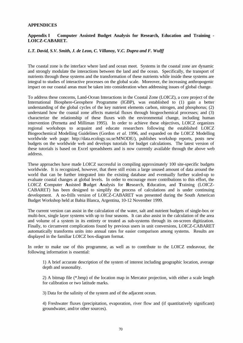
70

APPENDICES

Appendix I Computer Assisted Budget Analysis for Research, Education and Training -LOICZ-CABARET.

L.T. David, S.V. Smith, J. de Leon, C. Villanoy, V.C. Dupra and F. Wulff

The coastal zone is the interface where land and ocean meet. Systems in the coastal zone are dynamicand strongly modulate the interactions between the land and the ocean. Specifically, the transport ofnutrients through these systems and the transformation of these nutrients while inside these systems areintegral to studies of interactive processes on the global scale. Moreover, the increasing anthropogenicimpact on our coastal areas must be taken into consideration when addressing issues of global change.

To address these concerns, Land-Ocean Interactions in the Coastal Zone (LOICZ), a core project of theInternational Biosphere-Geosphere Programme (IGBP), was established to (1) gain a betterunderstanding of the global cycles of the key nutrient elements carbon, nitrogen, and phosphorus; (2)understand how the coastal zone affects material fluxes through biogeochemical processes; and (3)characterize the relationship of these fluxes with the environmental change, including humanintervention (Pernetta and Milliman 1995). In order to achieve these objectives, LOICZ organizesregional workshops to acquaint and educate researchers following the established LOICZBiogeochemical Modelling Guidelines (Gordon et al. 1996, and expanded on the LOICZ Modellingworldwide web page: http://data.ecology.su.se/MNODE/), publishes workshop reports, posts newbudgets on the worldwide web and develops tutorials for budget calculations. The latest version ofthese tutorials is based on Excel spreadsheets and is now currently available through the above webaddress.

These approaches have made LOICZ successful in compiling approximately 100 site-specific budgetsworldwide. It is recognized, however, that there still exists a large unused amount of data around theworld that can be further integrated into the existing database and eventually further scaled-up toevaluate coastal changes at global levels. In order to encourage more contributions to this effort, theLOICZ Computer Assisted Budget Analysis for Research, Education, and Training (LOICZ-CABARET) has been designed to simplify the process of calculations and is under continuingdevelopment. A no-frills version of LOICZ-CABARET was presented during the South AmericanBudget Workshop held at Bahia Blanca, Argentina, 10-12 November 1999.

The current version can assist in the calculation of the water, salt and nutrient budgets of single-box ormulti-box, single layer systems with up to four seasons. It can also assist in the calculation of the areaand volume of a system in its entirety or treated as sub-systems through its on-screen digitization.Finally, to circumvent complications found by previous users in unit conversions, LOICZ-CABARETautomatically transforms units into annual rates for easier comparison among systems. Results aredisplayed in the familiar LOICZ box-diagram format.

In order to make use of this programme, as well as to contribute to the LOICZ endeavour, thefollowing information is essential:

1) A brief accurate description of the system of interest including geographic location, averagedepth and seasonality.

2) A bitmap file (*.bmp) of the location map in Mercator projection, with either a scale lengthfor calibration or two latitude marks.

3) Data for the salinity of the system and of the adjacent ocean.

4) Freshwater fluxes (precipitation, evaporation, river flow and (if quantitatively significant)groundwater, and/or other sources).

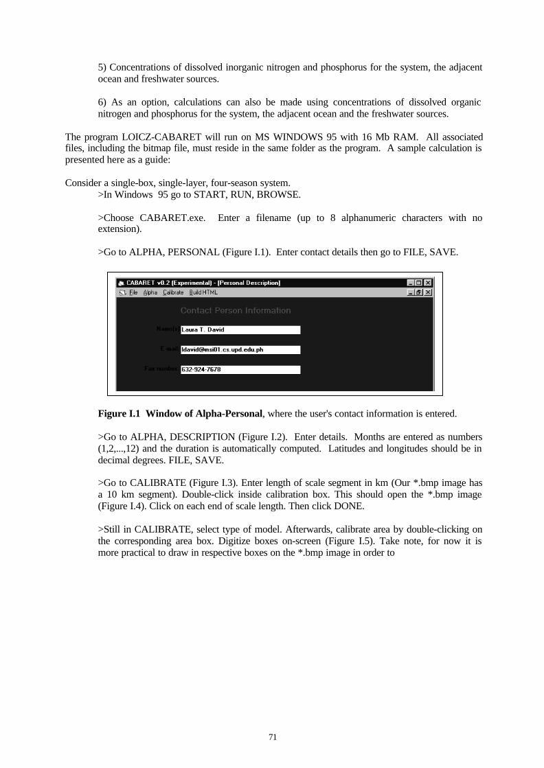
71

5) Concentrations of dissolved inorganic nitrogen and phosphorus for the system, the adjacentocean and freshwater sources.

6) As an option, calculations can also be made using concentrations of dissolved organicnitrogen and phosphorus for the system, the adjacent ocean and the freshwater sources.

The program LOICZ-CABARET will run on MS WINDOWS 95 with 16 Mb RAM. All associatedfiles, including the bitmap file, must reside in the same folder as the program. A sample calculation ispresented here as a guide:

Consider a single-box, single-layer, four-season system.>In Windows 95 go to START, RUN, BROWSE.

>Choose CABARET.exe. Enter a filename (up to 8 alphanumeric characters with noextension).

>Go to ALPHA, PERSONAL (Figure I.1). Enter contact details then go to FILE, SAVE.

Figure I.1 Window of Alpha-Personal, where the user's contact information is entered.

>Go to ALPHA, DESCRIPTION (Figure I.2). Enter details. Months are entered as numbers(1,2,...,12) and the duration is automatically computed. Latitudes and longitudes should be indecimal degrees. FILE, SAVE.

>Go to CALIBRATE (Figure I.3). Enter length of scale segment in km (Our *.bmp image hasa 10 km segment). Double-click inside calibration box. This should open the *.bmp image(Figure I.4). Click on each end of scale length. Then click DONE.

>Still in CALIBRATE, select type of model. Afterwards, calibrate area by double-clicking onthe corresponding area box. Digitize boxes on-screen (Figure I.5). Take note, for now it ismore practical to draw in respective boxes on the *.bmp image in order to

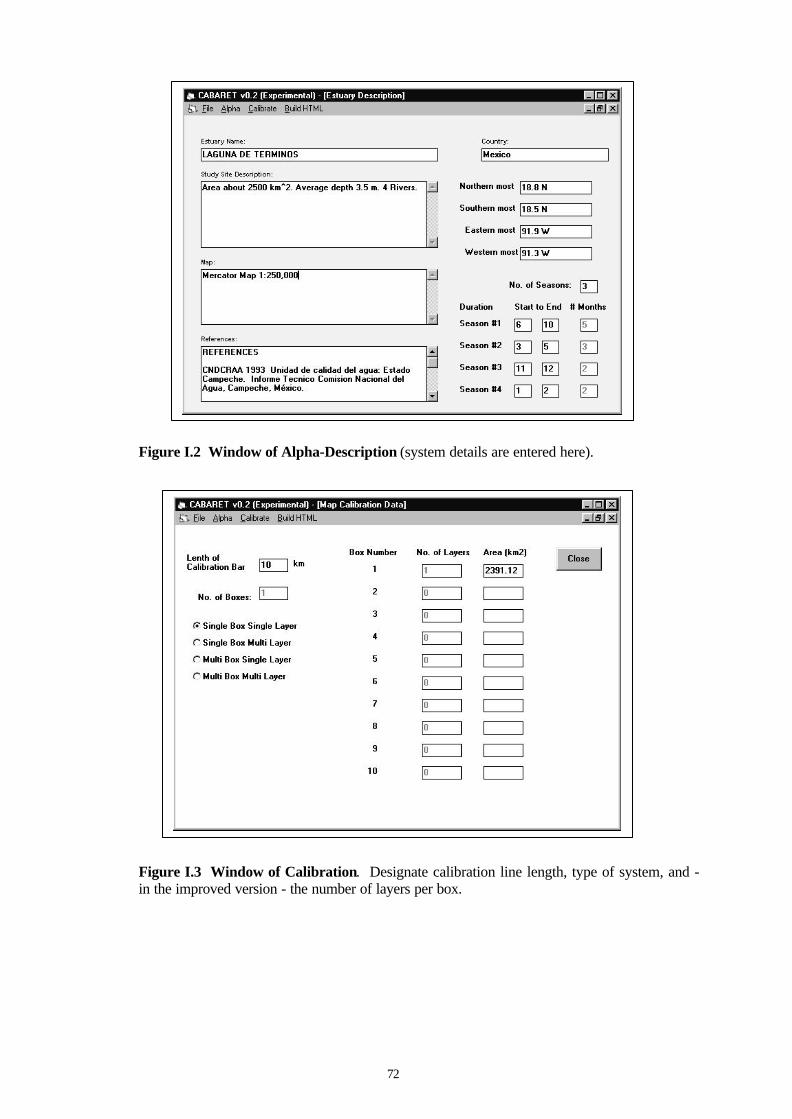
72

Figure I.2 Window of Alpha-Description (system details are entered here).

Figure I.3 Window of Calibration. Designate calibration line length, type of system, and -in the improved version - the number of layers per box.

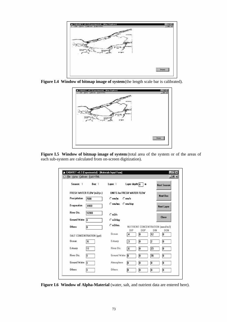
73

Figure I.4 Window of bitmap image of system (the length scale bar is calibrated).

Figure I.5 Window of bitmap image of system (total area of the system or of the areas ofeach sub-system are calculated from on-screen digitization).

Figure I.6 Window of Alpha-Material (water, salt, and nutrient data are entered here).

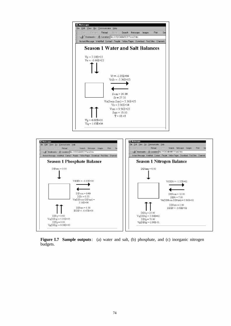
74

Figure I.7 Sample outputs : (a) water and salt, (b) phosphate, and (c) inorganic nitrogenbudgets.

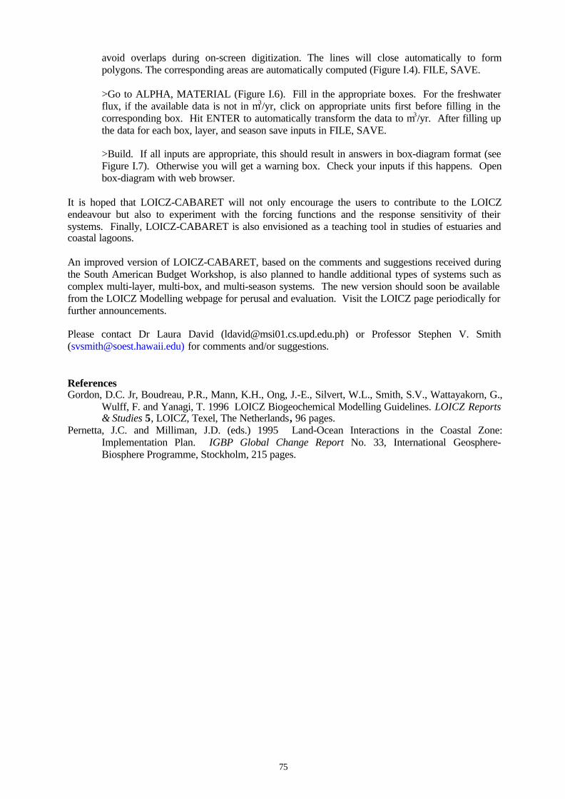
75

avoid overlaps during on-screen digitization. The lines will close automatically to formpolygons. The corresponding areas are automatically computed (Figure I.4). FILE, SAVE.

>Go to ALPHA, MATERIAL (Figure I.6). Fill in the appropriate boxes. For the freshwaterflux, if the available data is not in m3/yr, click on appropriate units first before filling in thecorresponding box. Hit ENTER to automatically transform the data to m3/yr. After filling upthe data for each box, layer, and season save inputs in FILE, SAVE.

>Build. If all inputs are appropriate, this should result in answers in box-diagram format (seeFigure I.7). Otherwise you will get a warning box. Check your inputs if this happens. Openbox-diagram with web browser.

It is hoped that LOICZ-CABARET will not only encourage the users to contribute to the LOICZendeavour but also to experiment with the forcing functions and the response sensitivity of theirsystems. Finally, LOICZ-CABARET is also envisioned as a teaching tool in studies of estuaries andcoastal lagoons.

An improved version of LOICZ-CABARET, based on the comments and suggestions received duringthe South American Budget Workshop, is also planned to handle additional types of systems such ascomplex multi-layer, multi-box, and multi-season systems. The new version should soon be availablefrom the LOICZ Modelling webpage for perusal and evaluation. Visit the LOICZ page periodically forfurther announcements.

Please contact Dr Laura David ([email protected]) or Professor Stephen V. Smith([email protected]) for comments and/or suggestions.

ReferencesGordon, D.C. Jr, Boudreau, P.R., Mann, K.H., Ong, J.-E., Silvert, W.L., Smith, S.V., Wattayakorn, G.,

Wulff, F. and Yanagi, T. 1996 LOICZ Biogeochemical Modelling Guidelines. LOICZ Reports& Studies 5, LOICZ, Texel, The Netherlands, 96 pages.

Pernetta, J.C. and Milliman, J.D. (eds.) 1995 Land-Ocean Interactions in the Coastal Zone:Implementation Plan. IGBP Global Change Report No. 33, International Geosphere-Biosphere Programme, Stockholm, 215 pages.

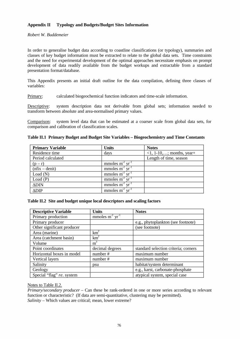
76

Appendix II Typology and Budgets/Budget Sites Information

Robert W. Buddemeier

In order to generalise budget data according to coastline classifications (or typology), summaries andclasses of key budget information must be extracted to relate to the global data sets. Time constraintsand the need for experimental development of the optimal approaches necessitate emphasis on promptdevelopment of data readily available from the budget workups and extractable from a standardpresentation format/database.

This Appendix presents an initial draft outline for the data compilation, defining three classes ofvariables:

Primary: calculated biogeochemical function indicators and time-scale information.

Descriptive: system description data not derivable from global sets; information needed totransform between absolute and area-normalised primary values.

Comparison: system level data that can be estimated at a coarser scale from global data sets, forcomparison and calibration of classification scales.

Table II.1 Primary Budget and Budget Site Variables – Biogeochemistry and Time Constants

Primary Variable Units NotesResidence time days <1, 1-10,…; months, year+Period calculated Length of time, season(p – r) mmoles m-2 yr-1

(nfix – denit) mmoles m-2 yr-1

Load (N) mmoles m-2 yr-1

Load (P) mmoles m-2 yr-1

∆DIN mmoles m-2 yr-1

∆DIP mmoles m-2 yr-1

Table II.2 Site and budget unique local descriptors and scaling factors

Descriptive Variable Units NotesPrimary production mmoles m-2 yr-1

Primary producer e.g., phytoplankton (see footnote)Other significant producer (see footnote)Area (marine) km2

Area (catchment basin) km2

Volume m3

Point coordinates decimal degrees standard selection criteria; cornersHorizontal boxes in model number # maximum numberVertical layers number # maximum numberSalinity psu habitat/system determinantGeology e.g., karst, carbonate-phosphateSpecial “flag” re. system atypical system, special case

Notes to Table II.2.Primary/secondary producer – Can these be rank-ordered in one or more series according to relevantfunction or characteristic? (If data are semi-quantitative, clustering may be permitted).Salinity – Which values are critical; mean, lower extreme?

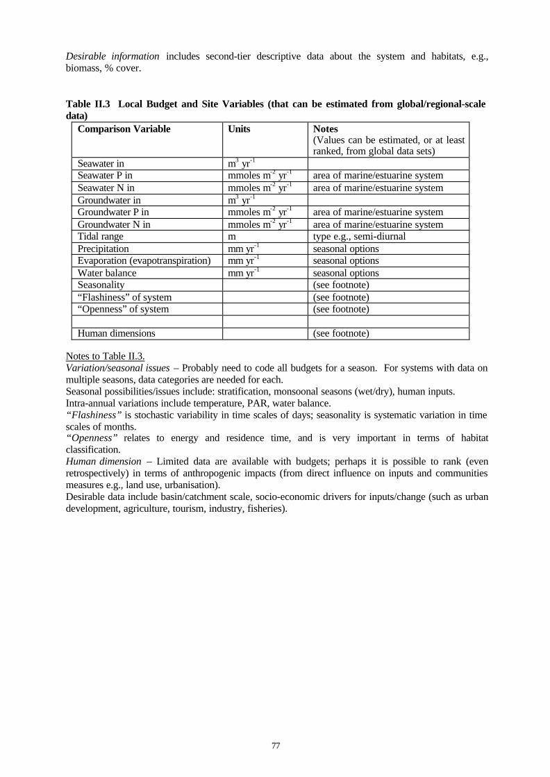
77

Desirable information includes second-tier descriptive data about the system and habitats, e.g.,biomass, % cover.

Table II.3 Local Budget and Site Variables (that can be estimated from global/regional-scaledata)

Comparison Variable Units Notes(Values can be estimated, or at leastranked, from global data sets)

Seawater in m3 yr-1

Seawater P in mmoles m-2 yr-1 area of marine/estuarine systemSeawater N in mmoles m-2 yr-1 area of marine/estuarine systemGroundwater in m3 yr-1

Groundwater P in mmoles m-2 yr-1 area of marine/estuarine systemGroundwater N in mmoles m-2 yr-1 area of marine/estuarine systemTidal range m type e.g., semi-diurnalPrecipitation mm yr-1 seasonal optionsEvaporation (evapotranspiration) mm yr-1 seasonal optionsWater balance mm yr-1 seasonal optionsSeasonality (see footnote)“Flashiness” of system (see footnote)“Openness” of system (see footnote)

Human dimensions (see footnote)

Notes to Table II.3.Variation/seasonal issues – Probably need to code all budgets for a season. For systems with data onmultiple seasons, data categories are needed for each.Seasonal possibilities/issues include: stratification, monsoonal seasons (wet/dry), human inputs.Intra-annual variations include temperature, PAR, water balance.“Flashiness” is stochastic variability in time scales of days; seasonality is systematic variation in timescales of months.“Openness” relates to energy and residence time, and is very important in terms of habitatclassification.Human dimension – Limited data are available with budgets; perhaps it is possible to rank (evenretrospectively) in terms of anthropogenic impacts (from direct influence on inputs and communitiesmeasures e.g., land use, urbanisation).Desirable data include basin/catchment scale, socio-economic drivers for inputs/change (such as urbandevelopment, agriculture, tourism, industry, fisheries).

78

Appendix III Workshop Report

WelcomeParticipants (Appendix IV) were welcomed to the Instituto Argentino de Oceanografia in BahiaBlanca, Argentina by Dr Gerardo Perillo. The workshop leader, Prof. Stephen Smith, convened theworkshop and, following a round-table introduction of participants, provided an outline of the purposeof the workshop and expected outcomes. The issues of publication and website use were addressed,and the mechanisms and processes for continuing regional training and budgets development weredescribed. The agenda (Appendix V) was introduced and working documents and diskettes ofelectronic information and tutorial materials were distributed.

Introduction and BackgroundThe LOICZ goals and approaches were presented by Dr Chris Crossland, and a context for theWorkshop outcomes was provided against the broad questions of the Programme. The joint support ofUNEP and financial assistance of GEF were acknowledged and the global biogeochemical budgets-typology project was outlined. Emphasis was given to the central questions of evaluating materialfluxes, the influence of the human dimension on global changes in process and function within thecoastal zone, and the use of typological tools to develop a global picture of system responses andchange.

Prof Fred Wulff and Mr Dennis Swaney described and illustrated the LOICZ Modelling website,explaining its vital use and function as a publication focus for the global biogeochemistry siteevaluations. The dynamic nature of information and the author attribution elements were emphasised.Existing and planned developments for the site, including tutorial materials, were outlined.

A prototype electronic programme for calculation and assessment of site-specific local budgets wasprovided to participants and demonstrated by Dr Laura David. The CABARET program (ComputerAssisted Budget Analysis for Research, Education and Training, see Appendix I) is being developed aspart of the UNEP/GEF project, and the current version was discussed and trialled by participants.Further developments are underway to include a rigorous multiple-box, multiple-layer and multiple-season capability with user-friendly tutorial background. The programme was well-received byparticipants as a valuable tool. Feedback from the workshop participants on ease of use andunderstandability are to be incorporated.

Prof. Smith outlined the tools that have been developed and information available from previousworkshops, making participants aware of support materials which can contribute to budgetcalculations, including: assessment of errors and sensitivity of the LOICZ approach (LOICZ R&S 12,1999), estimation of groundwater by silicate proxy (LOICZ R&S 13, 1999), run-off calculations andwaste-water analyses (LOICZ R&S 14, in press). These tools also are available on the LOICZModelling website.

The Regional Mentor for the Latin American region, Dr Victor Camacho, outlined the role of theregional mentor in continuing training, education and as a focal point for further development ofestuarine budgets throughout the region. The position (along with similar appointments in two otherregions of the world) has been established under the UNEP GEF project and will further encourageawareness and contribution to the project efforts in describing the global nutrient flux changes. DrCamacho demonstrated the use of the LOICZ modelling approach using the San Quintin model as atraining example, showing its evolution with increased data through time and its application as a toolfor addressing socio-economic issues and coastal zone management.

The LOICZ-developed coastal typology (or classification) approach was described by Dr RobertBuddemeier, emphasising application of the approach to the question of scaling and integration to meetregional and global needs for assessment of material flux changes. The approach allows measuredproxy information to be applied to unmeasured sites and regions leading to an ability for up-scaling andprediction of systems performance. Key elements were considered, including: standardisation of datasets, proxy development, algorithms for scaling and weighting of parameters, and sensitivity analyses

79

and variables. Some initial products relevant to the region provided an illustration of application of theapproach.

Presentation of Biogeochemical BudgetsThe contributing budgets brought by the participants were briefly considered, including an overview ofthe system settings, data availability and quality, approaches being taken to build budgets, and thestatus and problems in making the model assessments. System sites included:

BrazilAraruama LagoonCamboriu River estuaryMarica-Guarapina Lagoon and estuaryParanagua BayPiaui River estuaryPiratininga-Itaipu coastal lagoonsSergipe RiverUruguayRio de la PlataArgentinaBahia NuevaEcuadorGuayaquil GulfChileAysen Sound

Budgets DevelopmentBreak-out groups worked interactively on the development of these site budgets, supplemented withmethodological and site/issue-based tutorials and discussions. Estimates for sites and evolution ofassessment approaches were made, and budgets refinement emerged from resolution of techniques,application of derivative data and assessment of watershed information.

Plenary and discussion sessions were held throughout the workshop. These enabled review of thestatus of budgets development and discussion of key issues raised by participants, as well as alliedtopics, such as: C:N:P ratio and stoichiometry, limits and “reasonable” values in budget assessments,scaling variables and typology (see Appendix II).

Outcomes and Wrap-upBudgets for all systems were developed to a final or interim draft stage of completion during theworkshop; additions to text descriptions and a check on data sources were required by most budgetsbefore final contribution. A schedule for contribution and publication of the printed and CD-ROMreport, and posting to the LOICZ website, was agreed.

A number of additional sites was identified for which data is available and which may yield budgets.Participants committed to making other site budgets, subject to data availability, and to encourageothers to make further site assessments. A national training workshop was foreshadowed forColombia, based on discussions with national research leaders during the associated LOICZ OpenScience Meeting. The workshop will be run by the Regional Mentor and is expected to involve severaladditional scientists from Chile. Mr Weber Landim de Sousa is expected to spend 4-6 weeks at theUniversidad Autonoma de Baja California, Mexico, working with the Regional Mentor, Dr Camacho,on allied system analyses (subject to organisational agreement), and supported by the LOICZ/UNEPRegional Training Scholarship (South America).

The participants joined with LOICZ in expressing thanks to Dr Gerardo Perillo and his group from theInstituto Argentino de Oceanografia for support and hosting of the workshop in Bahia Blanca. Thefinancial support of the Global Environment Facility was gratefully acknowledged.

80

Appendix IV List of Participants and Contributing Authors

External Resource PersonsDr Robert W. BuddemeierKansas Geological SurveyUniversity of Kansas1930 Constant AveLawrence, Kansas 66047-3720USAphone +1 785 864 3965fax +1 785 864 [email protected]

Dr Paul BoudreauDepartment of Fisheries and OceansBedford Institute of OceanographyPO Box 1006Dartmouth, Nova Scotia B2Y 4A2,CANADAPhone: +1 902 426 7464Fax: +1 902 426 [email protected]

Dr Victor Camacho-IbarInstituto de Investigaciones OceanológicasUniversidad Autónoma de Baja CaliforniaApartado Postal 453Ensenada, Baja California 22860MEXICOphone +52 61 744601 x 123fax +52 61 [email protected]

Dr Chris J. CrosslandLOICZ International Project OfficeNetherlands Institute for Sea ResearchPO Box 591790 AB Den Burg, TexelTHE NETHERLANDSphone +31 222 69404fax +31 222 [email protected]

Dr Laura DavidMarine Science InstituteUniversity of the PhilippinesRoces Ave, Diliman, Quezon CityPHILIPPINESTel +63 2 922 3544Fax +63 2 924 [email protected]@msi01.cs.upd.edu.ph

Vilma DupraSchool of Ocean and Earth Science and

TechnologyUniversity of Hawaii1000 Pope RoadHonolulu, Hawaii 96822USAphone +1 808 956 2354fax +1 808 956 [email protected]

Prof. Stephen V. SmithSchool of Ocean and Earth Science and

TechnologyUniversity of Hawaii1000 Pope RoadHonolulu, Hawaii 96822USAphone +1 808 956 8693fax +1 808 956 [email protected]

Dennis SwaneyBoyce Thompson Institute for Plant ResearchTower RdCornell UniversityIthaca, New York 14853USAphone +1 607 524 [email protected]

Prof. Fred WulffDepartment of Systems EcologyUniversity of Stockholm106 91 StockholmSWEDENphone +46 8 16 42 50fax +46 8 15 84 [email protected]

Regional ParticipantsArgentinaDr J.L. EstevesCentro Nacional Patagónico (CONICET)Bv. Brown 3000 (9120)Puerto Madryn, ChubutARGENTINAphone +54 2965 451024, 451026fax +54 2965 [email protected]

81

Monica Noemi GilCentro Nacional Patagónico (CONICET)Bv. Brown 3000 (9120)Puerto Madryn, ChubutARGENTINAphone: 54 2965 451024, 451026fax: 54 2965 [email protected]

BrazilErminda C. G. CoutoUniversidade Federal de SergipeDepartamento de BiologiaCampus UniversitárioJardim Rosa ElzeSão Cristóvão SergipeCEP49100-000BRAZILphone +55 79 212 6693fax =55 79 212 [email protected]

Jurandir Pereira FilhoCTT Mar, Universidade do Vale do ItajaiR. Uruguai 458Itasai -Sc.88302-202 Itajai SCBRAZILphone +55 47 341 7633fax +55 47 341 [email protected]

Marcelo F. Landim de SouzaDepartamento de Ciências Exactas e

TecnológicasUniversidade Estadual de Santa CruzCEP 45.650-000BRAZILphone +55 73 680 [email protected]@[email protected]

Weber Friederichs Landim de SouzaUniversidade Federal FluminensePrograma de GeoquímicaMorro do Valonguinho, s/n Centro-NiteróiRio de JaneiroCEP 24020-007BRAZILphone +55 21 620 1313fax +55 21 620 [email protected]@altavista.net

Eunice de Costa MachadoUniversidade Federal Do Parana - Centro De

Estodos do MarAv. Beiramar Sin, Pontal DosulPontal Do Parana83255000-PRBRAZILphone +55 41 455 1333fax +55 41 455 1105e-mail: [email protected]

ChileNelson Silva S.Escuela de Ciencias del MarUniversidad Católica de ValparaísoCasilla 1020 ValparaísoCHILEPhone +56 32 274246Fax +56 32 [email protected]

Isabel Tutivén UbillaFacultad de Ciebcias Naturales y OceanografíaUniversidad de ConcepciónCasilla 160-C, ConcepciónCHILEPhone +56 41 204 239/230 929Fax +56 41 [email protected]

UruguayDr Gustavo J. NagyPCMYAFacultad de CienciasIgua 4225MontevideoURUGUAYfax +59 82 525 [email protected]

82

Contributing AuthorsBrazilRegina Celia Bastos AndradeUniversidade Federal FluminensePrograma de Pos-Graduacao em GeoquimicaNiteroi RJCEP 24.007-000BRAZILDr Bastiaan Adriaan KnoppersUniversidade Federal FluminensePrograma de Pos-Graduacao em GeoquimicaNiteroi RJCEP 24.007-000BRAZIL

Simone Santana de FreitasUniveridade Federal de SergipeDepartamento de Engenharia QuimicaSao Cristovao SECEP 49.100-000BRAZIL

Vivianne Ramos GomesUniversidade Federal de SergipeDepartamento de Engenharia QuimicaSao Cristovao SECEP 49.100-000BRAZIL

R.M. LopesCentre for Marine StudiesUniversidade Federal do ParanaAv. Beira Mar s/nPontal do Parana PR83255-000BRAZIL

Dr Eduardo MaroneCentre for Marine StudiesUniversidade Federal do ParanaAv. Beira Mar s/nPontal do Parana PR83255-000BRAZIL

E.T. SilvaCentre for Marine StudiesUniversidade Federal do ParanaAv. Beira Mar s/nPontal do Parana PR83255-000BRAZIL

Carlos Augustos SchettiniCtt. Mar/UnivaliR. Uruguai, 458Itasai -Sc.88302-202BRAZIL

Nicole A.C. ZyngierUniversidade Federal de SergipeDepartamento de BiologiaCampus UniversitárioJardim Rosa ElzeSão Cristóvão SergipeCEP49100-000BRAZIL

ChileDafne Guzman Z.Escuela de Ciencias del MarUniversidad Católica de ValparaísoValparaísoCHILE

Alexander Valdenegro M.Escuela de Ciencias del MarUniversidad Católica de ValparaísoValparaísoCHILE

PhilippinesJ. de LeonMarine Science InstituteUniversity of the PhilippinesQuezon CityPHILIPPINES

C.VillanoyMarine Science InstituteUniversity of the PhilippinesQuezon CityPHILIPPINES

83

Appendix V Workshop Agenda

South America Biogeochemical Budgeting WorkshopBahia Blanca

10-12 November 1999

Wednesday, November 100830 Convene Workshop - Stephen Smith

General greeting and introduction to Bahia Blanca - Gerardo PerilloGeneral housekeeping, introductions - Chris CrosslandIntroduction to LOICZ and GEF - Chris CrosslandIntroduction to LOICZ web pages - Dennis SwaneyPresentation of CABARET (Computer Assisted Biogeochemical Analysis, Research, Educationand Training) - Laura David

1030 Coffee Break

1100 Introduction to typology: what, why, and how - Bob Buddemeier

Begin brief (<10 minutes each) presentations of budgets: Give general site information (location,size, important characteristics), budget status (not details; we want to know the following:finished? problems? questions?) – participants.

1230 Lunch

1400 Convene for afternoon. Continue presentations, as needed.

1500 Plenary discussion to “see where we are at.” Identify data for additional budgets, work onsynthesis and typology. Resource persons work with one or more tutorial groups, as needed.

1530 Coffee

1600 Continue, as appropriate, until 1730. The remainder of the schedule for this afternoon and the nexttwo days is largely set by the outcome of the Wednesday afternoon plenary.

Thursday, November 110900-1700 Breakout groups or plenary, as required, to refine and present budgets. Coffee and lunch

breaks and discussion as above.

Friday, November 120900-1230 Break out groups and plenary, to develop preliminary synthesis.1230-1330 Lunch break and discussion.1330-1630 Afternoon: Plenary wrap-up discussion (Chair: S. Smith).1630-1730 Closing announcements (S. Smith & others, as needed).

The session times for each day will be as laid out here, for organizational convenience, unless there provesto be good reason to change them.

We will, as a minimum, have a 15-minute plenary each morning and at the end of each morning andafternoon session to update our status.

84

All “promised budgets” that were your basis for admission to the workshop should be turned in, onelectronic copy, to Vilma Dupra before the end of the day on November 12. Submissions this week shouldbe near-final versions, with no more than very minor repairs that will need to be made and emailed to us nolater than December 1.

If, as a result of discussion, persons agree to furnish materials beyond their promised budgets (additionalbudgets, appendix material, or other writing assignments), these materials will need to be in hand no laterthan January 1.

85

Appendix VI Terms of Reference for Workshop

TERMS OF REFERENCELOICZ/UNEP WORKSHOP ON

ESTUARINE SYSTEMS OF THE SOUTH AMERICAN REGIONInstituto Argentino de Oceanografia

Bahia Blanca, Argentina10-12 November 1999

Primary Goals:To work with researchers dealing with estuarine systems of the South American region, in order to extractC,N and P budgetary information from as many systems as feasible from existing data. The SouthAmerican systems extend around some of the perimeter of two of the Earth's major oceans. Moreover,many of these estuarine systems have relatively detailed data. The workshop provides the opportunity tocharacterize terrigenous inputs to the estuaries of the region, and outputs from the estuaries - hence the netrole of the estuarine zone of this region as a source or sink for carbon, nitrogen, and phosphorus.

This workshop will complement earlier, successful workshops in Ensenada, Mexico, in June 1997, asecond Mexican workshop in January 1999 (Merida, Mexico), an Australasian workshop (Canberra,Australia) in October 1998, and a South China Sea region workshop (Manila, the Philippines) in July 1999.

It is hoped that each workshop participant will be able to bring the data for at least two budgets: one froma “pollution hot spot” region within his/her country, and one from a physiographically fairly similar regionwhich is apparently subjected to less pollution. By this strategy, we hope to compile a set of sites that willrepresent a relatively wide range of human pressures in the South American region.

It is expected that further work on biogeochemical budget approaches will be generated in the region as aresult of the products and training components of this workshop.

Anticipated Products:1. Develop budgets for as many systems as feasible during the workshop.2. Examine other additional data, brought by the researchers or provided in advance, to scope out

how many additional systems can be budgeted over an additional 2 months.3. Prepare a LOICZ technical report and a CD-ROM summarizing this information.4. Contribute data/budgets from these sites to 1-2 papers to be published in the refereed scientific

literature.5. It is anticipated that one participant from the workshop will be offered the opportunity to spend up

to two months, probably in either Hawaii or Stockholm, getting further experience and developingadditional budgets for the region.

Participation:The number of participants will be limited to fewer than 18, to allow the active involvement of allparticipants. Nominees include:• External resource persons (Stephen Smith, Vilma Dupra, Laura David, Chris Crossland);• Approximately 13 researchers from the region (see below).

86

Workplan:Participants will be expected to come prepared to participate in discussions on coastal budgets.Preparation should include reading the LOICZ Biogeochemical Modelling Guidelines (Gordon et al.1996), the Mexican Lagoons Workshop Report (Smith et al. 1997), examination of the budgets andtutorials presented on the LOICZ Modelling web page (http://data.ecology.su.se/MNODE/), and arrivingwith preliminary budgets, electronic maps and 1-3 page write-ups from “their” sites. In order to beincluded in the workshop report, the budgets should conform as closely as possible to the budgetingprotocol laid out in the above documentation.

Further Details:The primary seasonal pattern of the region is at least one wet season and one dry season per year. Ideally, abudget for each season would be developed. If a system is vertically stratified, then a 2-layer budget ispreferred over a single-layer budget. If a system has a strong land-to-sea salinity gradient, then it ispreferable to break the system along its length into several boxes.

Minimum data requirements to construct a satisfactory water and salt budget include: salinity of the systemand the adjacent ocean, runoff, rainfall, evaporation and (if likely to be important) inputs of otherfreshwater sources such as groundwater or sewage. Preferably, the salinity and freshwater inflow data arefor the same time period (for example, freshwater inflow data for a month or so immediately prior to theperiod of salinity measurement).

Minimum data requirements for the nutrient budgets are: concentrations of dissolved nutrients (phosphate,nitrate, ammonium and dissolved organic N and P if available) for the system and the adjacent ocean,concentrations of nutrients in in-flowing river water and (if important, in groundwater), some estimate ofnutrient (or at least BOD) loading from sewage or other waste discharges. If atmospheric deposition(particularly of N) is likely to be important, an estimate of this is also useful.

Workshop Schedule (All participants are expected to stay for the entire workshop):Nov 9: ArrivalNov 10: General introduction to the budgeting procedure and related issues; presentation of preliminary

budgets (no details, simply a quick summary to see who has what.)Breakout groups to revise, refine budgets. This will vary as needed from tutorial, throughdetailed help, to procedural discussions.

Nov 11: Continue breakouts; afternoon plenary to evaluate progress.Nov 12: Breakouts/plenary as required to develop synthesis.

Background Documents:1. Gordon, D.C., Boudreau, P.R., Mann, K.H., Ong, J.-E., Silvert, W., Smith, S.V., Wattayakorn, G.,

Wulff, F. and Yanagi T. 1996 LOICZ Biogeochemical Modelling Guidelines. LOICZ Reports andStudies 5, 96 pages.;

2. Smith, S.V., Ibarra-Obando, S., Boudreau, P.R. and Camacho-Ibar, V.F. 1997 Comparison of Carbon,Nitrogen and Phosphorus Fluxes in Mexican Coastal Lagoons. LOICZ Reports and Studies 10, 84pages.;

3. LOICZ Modelling web page, for everyone with www access: ( http://data.ecology.su.se/MNODE/ )

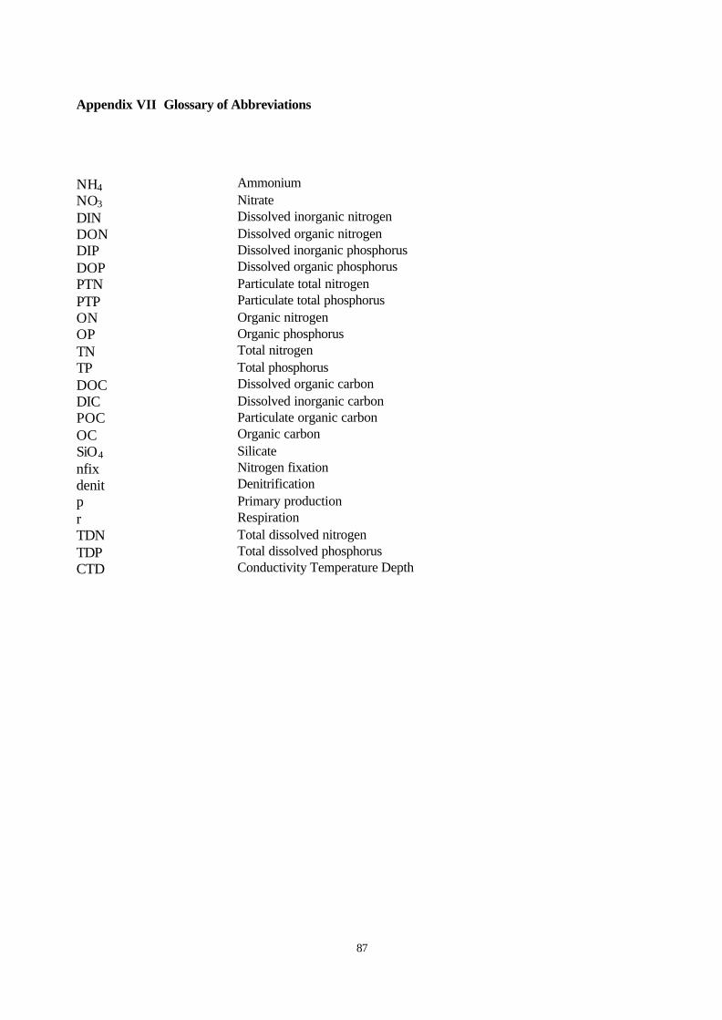
87

Appendix VII Glossary of Abbreviations

NH4 AmmoniumNO3 NitrateDIN Dissolved inorganic nitrogenDON Dissolved organic nitrogenDIP Dissolved inorganic phosphorusDOP Dissolved organic phosphorusPTN Particulate total nitrogenPTP Particulate total phosphorusON Organic nitrogenOP Organic phosphorusTN Total nitrogenTP Total phosphorusDOC Dissolved organic carbonDIC Dissolved inorganic carbonPOC Particulate organic carbonOC Organic carbonSiO4 Silicatenfix Nitrogen fixationdenit Denitrificationp Primary productionr RespirationTDN Total dissolved nitrogenTDP Total dissolved phosphorusCTD Conductivity Temperature Depth