Embed Size (px)
DESCRIPTION
Â
Citation preview
LAND-OCEAN INTERACTIONS IN THE COASTAL ZONE (LOICZ)
Core Project of theInternational Geosphere-Biosphere Programme: A Study of Global Change (IGBP)
Mexico Map showing lagoons
COMPARISON OF CARBON, NITROGEN AND PHOSPHORUS FLUXESIN MEXICAN COASTAL LAGOONS
LOICZ REPORTS & STUDIES No. 10
compiled and edited by S.V. Smith, S. Ibarra-Obando, P.R. Boudreau and V.F. Camacho-Ibar
LOICZ Core Project OfficeNetherlands Institute for Sea Research (NIOZ)
P.O. Box 59, 1790 AB Den Burg Texel, The Netherlands
Compiled & Edited by
Stephen V. SmithSchool of Ocean and Earth Science and Technology
Honolulu, Hawaii 96822United States of America
Silvia Ibarra-ObandoCenter for Scientific Research and Higher Education of Ensenada (CICESE)
EnsenadaBaja California, Mexico
Paul R. BoudreauLOICZ Core Project Office
Texel, The Netherlands
Víctor F. Camacho-IbarInstitución de Investigaciones Oceanológicas
Universidad Autónoma de Baja California(IIO-UABC)Ensenada
Baja California, Mexico
LOICZ REPORTS & STUDIES NO. 10
Published in the Netherlands, 1997 by:LOICZ Core ProjectNetherlands Institute for Sea ResearchP.O. Box 591790 AB Den Burg - TexelThe Netherlands
The Land-Ocean Interactions in the Coastal Zone Project is a Core Project of the “InternationalGeosphere-Biosphere Programme: A Study Of Global Change”, of the International Council ofScientific Unions.
The LOICZ Core Project is financially supported through the Netherlands Organisation for ScientificResearch by: the Ministry of Education, Culture and Science; the Ministry of Transport, Public Worksand Water Management; the Ministry of Housing, Planning and Environment; and the Ministry ofAgriculture, Nature Management and Fisheries of The Netherlands, as well as The Royal NetherlandsAcademy of Sciences, and The Netherlands Institute for Sea Research.
COPYRIGHT 1997, Land-Ocean Interactions in the Coastal Zone Core Project of the IGBP.
Reproduction of this publication for educational or other, non-commercial purposes isauthorised without prior permission from the copyright holder.
Reproduction for resale or other purposes is prohibited without the prior, writtenpermission of the copyright holder.
Citation: Smith, S.V., S. Ibarra-Obando, P.R. Boudreau and V.F. Camacho-Ibar. 1997.Comparison of Carbon, Nitrogen and Phosphorus Fluxes in Mexican Coastal Lagoons,LOICZ Reports & Studies No. 10, ii + 84 pp. LOICZ, Texel, The Netherlands.
ISSN: 1383-4304
Cover: Map of the coast of Mexico published in 1616. Note that, by this date, many lagoonsand coastal embayments were already being mapped along the Mexican coast.
Disclaimer: The designations employed and the presentation of the material contained in this reportdo not imply the expression of any opinion whatsoever on the part of LOICZ or theIGBP concerning the legal status of any state, territory, city or area, or concerning thedelimitation’s of their frontiers or boundaries. This report contains the views expressedby the authors and may not necessarily reflect the views of the IGBP.
The LOICZ Reports and Studies Series is published and distributed free of charge to scientistsinvolved in global change research in coastal areas.
- i -
TABLE OF CONTENTS
Page
1. OVERVIEW OF WORKSHOP AND BUDGET RESULTS 1
2. BUDGETS FOR MEXICAN COASTAL LAGOONS 4
2.1 Arid Pacific and Gulf of California coasts 42.1.1) Estero de Punta Banda, Baja California 42.1.2) Bahía San Quintín, Baja California (a teaching example) 92.1.3) Bahía San Luis Gonzaga, Baja California 162.1.4) Estero La Cruz, Sonora 212.1.5) Bahía Concepción, Baja California Sur 252.1.6) Ensenada de La Paz, Baja California Sur 29
2.2 Humid Pacific Coast 332.2.1) Bahía de Altata-Ensenada del Pabellón, Sinaloa 332.2.2)Teacapan-Agua Brava-Marismas Nacionales, Sinaloa and Nayarit 382.2.3) Carretas-Pereyra, Chiapas 432.2.4) Chantuto-Panzacola, Chiapas 47
2.3 Gulf of Mexico 512.3.1) Laguna Madre, Tamaulipas 512.3.2) Laguna de Terminos, Campeche 56
3. CONCLUSIONS AND IMPLICATIONS FOR LAGOON COMPARISON 60
4. REFERENCES 65
- ii -
APPENDICES
I MEXICAN COASTAL LAGOONS OVERVIEW 68
II COMPARISON OF NET & GROSS BUDGET FOR BAHÍA SAN QUINTÍN 71
III ECOLOGICAL SERVICES AND SOCIO-ECONOMIC SUSTAINABILITY 74 - A case study: Bahía San Quintín
IV SOCIO-ECONOMIC SITUATION OF LAGUNA DE TERMINOS 76
V MEXICAN LAGOONS WORKSHOP REPORT 77
VI LIST OF WORKSHOP PARTICIPANTS AND CONTRIBUTORS 82
VII WORKSHOP AGENDA 84
- 1 -
1. OVERVIEW OF WORKSHOP AND BUDGET RESULTS
A central and essential objective of the Land Ocean Interactions in the Coastal Zone (LOICZ) CoreProject of the International Geosphere-Biosphere Programme (IGBP) is to:
• gain a better understanding of the global cycles of the key nutrient elements carbon (C), nitrogen(N) and phosphorus (P);
• understand how the coastal zone affects these fluxes through biogeochemical processes; and,• characterise the relationship of these fluxes to human intervention (Pernetta and Milliman, 1995).
Coastal lagoons along the 12,000 km shoreline of Mexico are numerous, diverse, and well-studied.According to Contreras (1993) Mexico has about 180 coastal lagoons and other estuarine areas, withabout 10,000 km2 on the Pacific coast and 10,000 km2 on the Gulf of Mexico. These lagoons aresubject to extremely varied degrees and kinds of human pressure due to direct uses and indirectinsults. Considerable scientific information exists for many of these systems, and the bibliographicinformation has been well summarised (see References - Section 4). All of these considerations ledto the recognition by several members of the LOICZ Scientific Steering Committee that it would beappropriate to hold a regional workshop in order to develop budgets according to the LOICZBiogeochemical Modelling Guidelines (Gordon et al., 1996). Such a workshop seemed likely to yieldseveral useful budgets, to generate interest in the region in developing further budgets, and perhapsto provide a formula for generating regional budgets to be compiled into the world-wide databasebeing developed by the LOICZ Biogeochemical Modelling Node. That database is being posted on aWorld Wide Web Home Page (reachable through http://www.nioz.nl/loicz/modelnod). It was furtherrecognised that an understanding of the functioning of these diverse and well-studied Mexicanlagoons might be exported to other regions of the world with less well-studied lagoons.
The workshop was convened at the Center for Scientific Research and Higher Education ofEnsenada (CICESE) in Ensenada, Mexico, on June 2-3rd, 1997. Five resource persons (S. Smith, F.Wulff, R. Buddemeier, V. Camacho-Ibar and P. Boudreau) worked with eleven scientists from anumber of different institutions in Mexico. They were all familiar with lagoons throughout Mexico andbrought with them much of the necessary data and experience required to carry out the work. It was ahighly successful meeting that exceeded expectations and has laid a good framework for continuedstudies within the region.
Dr. S. Ibarra-Obando initiated the technical part of the workshop by presenting an overview of thenatural history of Mexican coastal zone. A synopsis of that overview is presented in Appendix I. Drs.Smith and Wulff presented an overview of the LOICZ budgeting procedure and used this workshopas the inaugural presentation of the Biogeochemical Modelling Home Page. Dr. Camacho-Ibarpresented a detailed budgetary analysis for Bahía San Quintín, Baja California, in order to guide theworkshop participants through the budgeting procedure. This budget represents an extension, basedon new (and more reliable) data, from the San Quintín budget originally presented in Gordon et al.(1996). Dr. Ibarra-Obando presented a comparison between the system-level budgets of net materialflux and addition of components to obtain gross turnover of materials (see Appendix II).
Following these general introductory exercises, the group broke into three working groups, looselystructured around hydrological regimes of the Mexican coastal zone:
Group 1 - Botello-Ruvalcaba, Boudreau, Camacho-Ibar, Delgadillo-Hinojosa, Lechuga-Devéze andPoumian-Tapia - derived budgets for five coastal lagoons in the desert region of Baja California, BajaCalifornia Sur, Sinaloa and Sonora.
Group 2 - Contreras-Espinosa, Flores-Verdugo, Ibarra-Obando, de la Lanza-Espino and Wulff -developed budgets for two coastal lagoon systems (each with several individual lagoons) in theregion with high-runoff in Nayarit, and Chiapas states.
Group 3 - Buddemeier, Carriquiry, Gomez-Reyes and Vázquez-Botello - developed a budget forLaguna de Terminos, Campeche, a large system lying in the transition region between the high runoffarea of the lower part of the Gulf of Mexico coast and the Yucatán Peninsula, which is dominated bylow surface runoff but high groundwater flow.
- 2 -
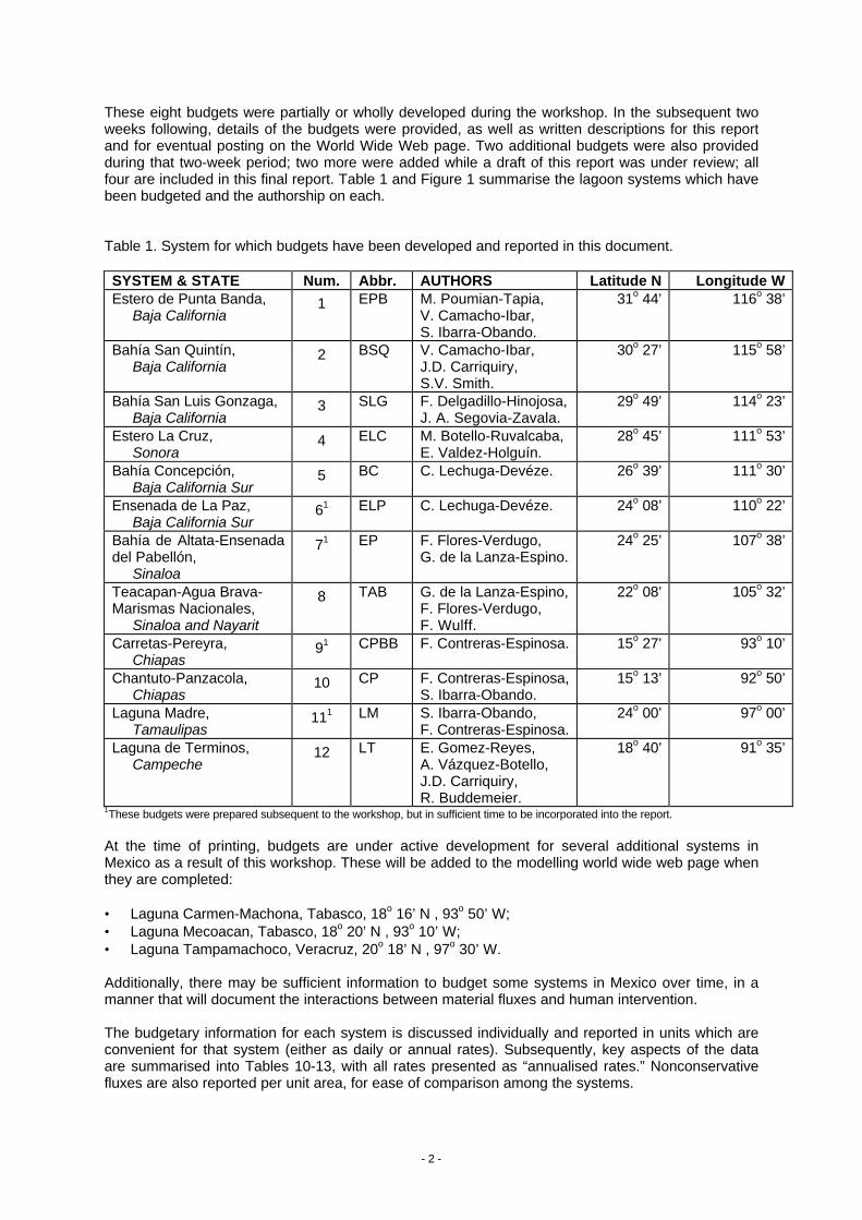
These eight budgets were partially or wholly developed during the workshop. In the subsequent twoweeks following, details of the budgets were provided, as well as written descriptions for this reportand for eventual posting on the World Wide Web page. Two additional budgets were also providedduring that two-week period; two more were added while a draft of this report was under review; allfour are included in this final report. Table 1 and Figure 1 summarise the lagoon systems which havebeen budgeted and the authorship on each.
Table 1. System for which budgets have been developed and reported in this document.
SYSTEM & STATE Num. Abbr. AUTHORS Latitude N Longitude WEstero de Punta Banda,
Baja California1 EPB M. Poumian-Tapia,
V. Camacho-Ibar,S. Ibarra-Obando.
31o 44’ 116o 38’
Bahía San Quintín,Baja California
2 BSQ V. Camacho-Ibar,J.D. Carriquiry,S.V. Smith.
30o 27’ 115o 58’
Bahía San Luis Gonzaga,Baja California
3 SLG F. Delgadillo-Hinojosa,J. A. Segovia-Zavala.
29o 49’ 114o 23’
Estero La Cruz,Sonora
4 ELC M. Botello-Ruvalcaba,E. Valdez-Holguín.
28o 45’ 111o 53’
Bahía Concepción,Baja California Sur
5 BC C. Lechuga-Devéze. 26o 39’ 111o 30’
Ensenada de La Paz,Baja California Sur
61 ELP C. Lechuga-Devéze. 24o 08’ 110o 22’
Bahía de Altata-Ensenadadel Pabellón,
Sinaloa
71 EP F. Flores-Verdugo,G. de la Lanza-Espino.
24o 25’ 107o 38’
Teacapan-Agua Brava-Marismas Nacionales,
Sinaloa and Nayarit
8 TAB G. de la Lanza-Espino,F. Flores-Verdugo,F. Wulff.
22o 08’ 105o 32’
Carretas-Pereyra,Chiapas
91 CPBB F. Contreras-Espinosa. 15o 27’ 93o 10’
Chantuto-Panzacola,Chiapas
10 CP F. Contreras-Espinosa,S. Ibarra-Obando.
15o 13’ 92o 50’
Laguna Madre,Tamaulipas
111 LM S. Ibarra-Obando,F. Contreras-Espinosa.
24o 00’ 97o 00’
Laguna de Terminos,Campeche
12 LT E. Gomez-Reyes,A. Vázquez-Botello,J.D. Carriquiry,R. Buddemeier.
18o 40’ 91o 35’
1These budgets were prepared subsequent to the workshop, but in sufficient time to be incorporated into the report.
At the time of printing, budgets are under active development for several additional systems inMexico as a result of this workshop. These will be added to the modelling world wide web page whenthey are completed:
• Laguna Carmen-Machona, Tabasco, 18o 16’ N , 93o 50’ W;• Laguna Mecoacan, Tabasco, 18o 20’ N , 93o 10’ W;• Laguna Tampamachoco, Veracruz, 20o 18’ N , 97o 30’ W.
Additionally, there may be sufficient information to budget some systems in Mexico over time, in amanner that will document the interactions between material fluxes and human intervention.
The budgetary information for each system is discussed individually and reported in units which areconvenient for that system (either as daily or annual rates). Subsequently, key aspects of the dataare summarised into Tables 10-13, with all rates presented as “annualised rates.” Nonconservativefluxes are also reported per unit area, for ease of comparison among the systems.

- 3 -
As useful steps towards relating the biogeochemical fluxes to human intervention, many of thedescriptions given here include socio-economic overviews. For two of these systems the socio-economic situations are explicitly discussed. Dr. S. Ibarra-Obando and others have laid out a briefoverview of socio-economic pressures imposed on the Bahía San Quintín and watershed system(Appendix III). Dr. A Vázquez-Botello has provided a brief synopsis of the competing human usesand pressures acting on Laguna de Terminos, the second largest Mexican lagoon (Appendix IV). It ishoped that these supporting documents, together with the biogeochemical budgets which are themain focus points of this report, will help provide framework for realistic integration betweenunderstanding material fluxes, which is the central theme of IGBP and LOICZ, the roles that humansplay in modifying those fluxes, and the implications of those modifications with respect to humans.
As another potentially useful product of this workshop, Dr. Gomez-Reyes has agreed to provide asimple and generalised method of dispersion analysis that can be used to estimate water exchangein lagoons and similar systems where there is no salt gradients between the lagoons and adjacentoceanic systems. This analysis will be added as a further link on the Biogeochemical ModellingHome Page.
The full meeting report, participants list and contact information is given in Appendix V and VI.
And a good time was had by all!
Figure 1. Map of Mexico showing names of coastal states and locations of budgeted lagoonalsystems. See Table 1 for system numbers.
- 4 -
2. BUDGETS FOR MEXICAN COASTAL LAGOONS
2.1 Arid Pacific and Gulf of California coasts
2.1.1 Estero de Punta Banda, Baja CaliforniaM. Poumian-Tapia, S. Ibarra-Obando and V. F. Camacho-Ibar
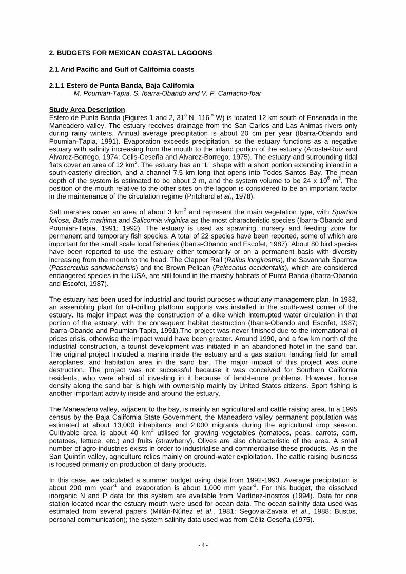
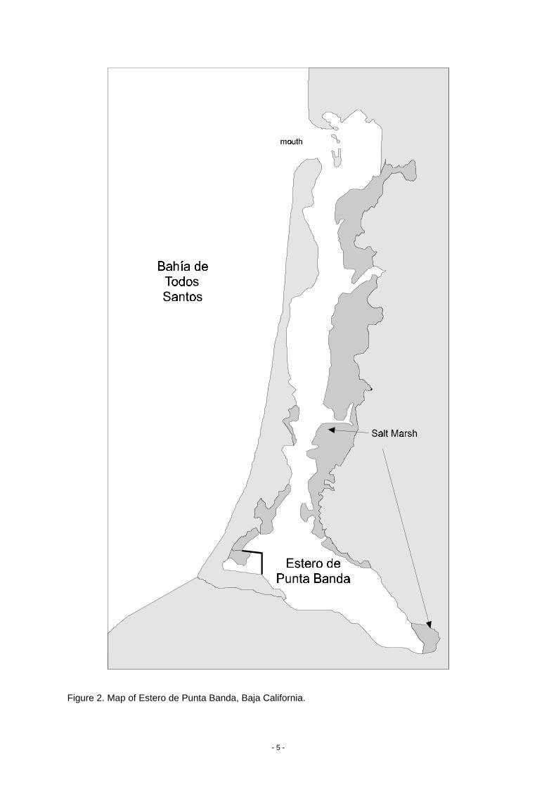
Study Area DescriptionEstero de Punta Banda (Figures 1 and 2, 31o N, 116 o W) is located 12 km south of Ensenada in theManeadero valley. The estuary receives drainage from the San Carlos and Las Animas rivers onlyduring rainy winters. Annual average precipitation is about 20 cm per year (Ibarra-Obando andPoumian-Tapia, 1991). Evaporation exceeds precipitation, so the estuary functions as a negativeestuary with salinity increasing from the mouth to the inland portion of the estuary (Acosta-Ruiz andAlvarez-Borrego, 1974; Celis-Ceseña and Alvarez-Borrego, 1975). The estuary and surrounding tidalflats cover an area of 12 km2. The estuary has an “L” shape with a short portion extending inland in asouth-easterly direction, and a channel 7.5 km long that opens into Todos Santos Bay. The meandepth of the system is estimated to be about 2 m, and the system volume to be 24 x 106 m3. Theposition of the mouth relative to the other sites on the lagoon is considered to be an important factorin the maintenance of the circulation regime (Pritchard et al., 1978).
Salt marshes cover an area of about 3 km2 and represent the main vegetation type, with Spartinafoliosa, Batis maritima and Salicornia virginica as the most characteristic species (Ibarra-Obando andPoumian-Tapia, 1991; 1992). The estuary is used as spawning, nursery and feeding zone forpermanent and temporary fish species. A total of 22 species have been reported, some of which areimportant for the small scale local fisheries (Ibarra-Obando and Escofet, 1987). About 80 bird specieshave been reported to use the estuary either temporarily or on a permanent basis with diversityincreasing from the mouth to the head. The Clapper Rail (Rallus longirostris), the Savannah Sparrow(Passerculus sandwichensis) and the Brown Pelican (Pelecanus occidentalis), which are consideredendangered species in the USA, are still found in the marshy habitats of Punta Banda (Ibarra-Obandoand Escofet, 1987).
The estuary has been used for industrial and tourist purposes without any management plan. In 1983,an assembling plant for oil-drilling platform supports was installed in the south-west corner of theestuary. Its major impact was the construction of a dike which interrupted water circulation in thatportion of the estuary, with the consequent habitat destruction (Ibarra-Obando and Escofet, 1987;Ibarra-Obando and Poumian-Tapia, 1991).The project was never finished due to the international oilprices crisis, otherwise the impact would have been greater. Around 1990, and a few km north of theindustrial construction, a tourist development was initiated in an abandoned hotel in the sand bar.The original project included a marina inside the estuary and a gas station, landing field for smallaeroplanes, and habitation area in the sand bar. The major impact of this project was dunedestruction. The project was not successful because it was conceived for Southern Californiaresidents, who were afraid of investing in it because of land-tenure problems. However, housedensity along the sand bar is high with ownership mainly by United States citizens. Sport fishing isanother important activity inside and around the estuary.
The Maneadero valley, adjacent to the bay, is mainly an agricultural and cattle raising area. In a 1995census by the Baja California State Government, the Maneadero valley permanent population wasestimated at about 13,000 inhabitants and 2,000 migrants during the agricultural crop season.Cultivable area is about 40 km2 utilised for growing vegetables (tomatoes, peas, carrots, corn,potatoes, lettuce, etc.) and fruits (strawberry). Olives are also characteristic of the area. A smallnumber of agro-industries exists in order to industrialise and commercialise these products. As in theSan Quintín valley, agriculture relies mainly on ground-water exploitation. The cattle raising businessis focused primarily on production of dairy products.
In this case, we calculated a summer budget using data from 1992-1993. Average precipitation isabout 200 mm year-1 and evaporation is about 1,000 mm year-1. For this budget, the dissolvedinorganic N and P data for this system are available from Martínez-Inostros (1994). Data for onestation located near the estuary mouth were used for ocean data. The ocean salinity data used wasestimated from several papers (Millán-Núñez et al., 1981; Segovia-Zavala et al., 1988; Bustos,personal communication); the system salinity data used was from Céliz-Ceseña (1975).
- 5 -
Figure 2. Map of Estero de Punta Banda, Baja California.
- 6 -
Water and Salt Balance
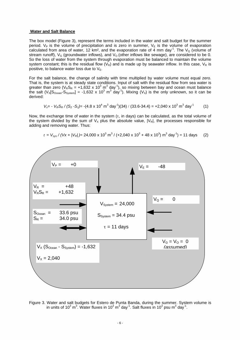
The box model (Figure 3), represent the terms included in the water and salt budget for the summerperiod. VP is the volume of precipitation and is zero in summer, VE is the volume of evaporationcalculated from area of water, 12 km², and the evaporation rate of 4 mm day-1. The VQ (volume ofstream runoff), VG (groundwater inflows), and VO (other inflows like sewage), are considered to be 0.So the loss of water from the system through evaporation must be balanced to maintain the volumesystem constant; this is the residual flow (VR) and is made up by seawater inflow. In this case, VR ispositive, to balance water loss due to VE.
For the salt balance, the change of salinity with time multiplied by water volume must equal zero.That is, the system is at steady state conditions. Input of salt with the residual flow from sea water isgreater than zero (VRSR = +1,632 x 103 m3 day-1), so mixing between bay and ocean must balancethe salt (VX[SOcean-SSystem] = -1,632 x 103 m3 day-1). Mixing (VX) is the only unknown, so it can bederived:
Vx= - VRSR / (S2 -S1)= -(4.8 x 10⁴ m3 day-1)(34) / (33.6-34.4) = +2,040 x 103 m3 day-1 (1)
Now, the exchange time of water in the system (τ, in days) can be calculated, as the total volume ofthe system divided by the sum of VX plus the absolute value, |VR|, the processes responsible foradding and removing water. Thus:
τ = Vsys / (Vx + |VR| )= 24,000 x 103 m3 / (+2,040 x 103 + 48 x 103) m3 day-1) = 11 days (2)
Figure 3. Water and salt budgets for Estero de Punta Banda, during the summer. System volume isin units of 103 m3. Water fluxes in 103 m3 day-1. Salt fluxes in 103 psu m3 day-1.
VQ = 0
VE = -48VP = +0
VSystem = 24,000
SSystem = 34.4 psu
τ = 11 days
VR = +48VRSR = +1,632
SOcean = 33.6 psuSR = 34.0 psu
VX (SOcean - SSystem) = -1,632
VX = 2,040
VG = VO = 0(assumed)
- 7 -
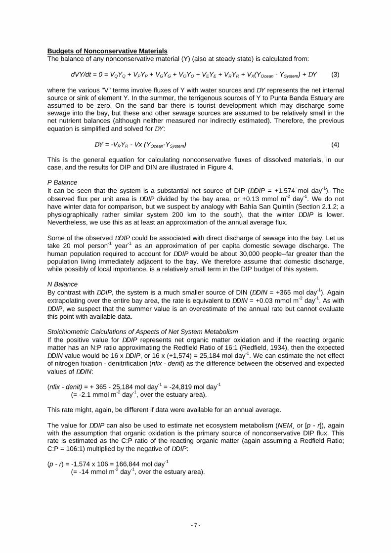
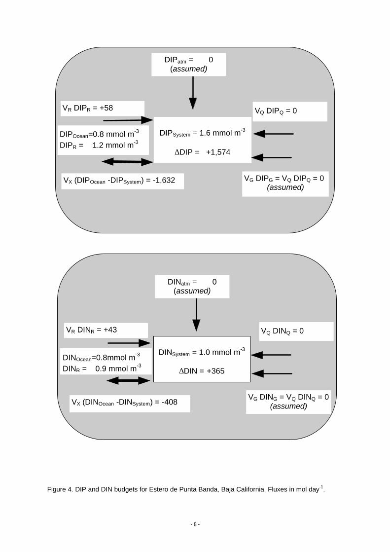
Budgets of Nonconservative MaterialsThe balance of any nonconservative material (Y) (also at steady state) is calculated from:
dVY/dt = 0 = VQYQ + VPYP + VGYG + VOYO + VEYE + VRYR + VX(YOcean - YSystem) + ∆Y (3)
where the various "V" terms involve fluxes of Y with water sources and ∆Y represents the net internalsource or sink of element Y. In the summer, the terrigenous sources of Y to Punta Banda Estuary areassumed to be zero. On the sand bar there is tourist development which may discharge somesewage into the bay, but these and other sewage sources are assumed to be relatively small in thenet nutrient balances (although neither measured nor indirectly estimated). Therefore, the previousequation is simplified and solved for ∆Y:
∆Y = -VRYR - Vx (YOcean-YSystem) (4)
This is the general equation for calculating nonconservative fluxes of dissolved materials, in ourcase, and the results for DIP and DIN are illustrated in Figure 4.
P BalanceIt can be seen that the system is a substantial net source of DIP (∆DIP = +1,574 mol day-1). Theobserved flux per unit area is ∆DIP divided by the bay area, or +0.13 mmol m-2 day-1. We do nothave winter data for comparison, but we suspect by analogy with Bahía San Quintín (Section 2.1.2; aphysiographically rather similar system 200 km to the south), that the winter ∆DIP is lower.Nevertheless, we use this as at least an approximation of the annual average flux.
Some of the observed ∆DIP could be associated with direct discharge of sewage into the bay. Let ustake 20 mol person-1 year-1 as an approximation of per capita domestic sewage discharge. Thehuman population required to account for ∆DIP would be about 30,000 people--far greater than thepopulation living immediately adjacent to the bay. We therefore assume that domestic discharge,while possibly of local importance, is a relatively small term in the DIP budget of this system.
N BalanceBy contrast with ∆DIP, the system is a much smaller source of DIN (∆DIN = +365 mol day-1). Againextrapolating over the entire bay area, the rate is equivalent to ∆DIN = +0.03 mmol m-2 day-1. As with∆DIP, we suspect that the summer value is an overestimate of the annual rate but cannot evaluatethis point with available data.
Stoichiometric Calculations of Aspects of Net System MetabolismIf the positive value for ∆DIP represents net organic matter oxidation and if the reacting organicmatter has an N:P ratio approximating the Redfield Ratio of 16:1 (Redfield, 1934), then the expected∆DIN value would be 16 x ∆DIP, or 16 x (+1,574) = 25,184 mol day-1. We can estimate the net effectof nitrogen fixation - denitrification (nfix - denit) as the difference between the observed and expectedvalues of ∆DIN:
(nfix - denit) = + 365 - 25,184 mol day-1 = -24,819 mol day-1
(= -2.1 mmol m-2 day-1, over the estuary area).
This rate might, again, be different if data were available for an annual average.
The value for ∆DIP can also be used to estimate net ecosystem metabolism (NEM¸ or [p - r]), againwith the assumption that organic oxidation is the primary source of nonconservative DIP flux. Thisrate is estimated as the C:P ratio of the reacting organic matter (again assuming a Redfield Ratio;C:P = 106:1) multiplied by the negative of ∆DIP:
(p - r) = -1,574 x 106 = 166,844 mol day-1
(= -14 mmol m-2 day-1, over the estuary area).
- 8 -
Figure 4. DIP and DIN budgets for Estero de Punta Banda, Baja California. Fluxes in mol day-1.
VQ DIPQ = 0
DIPatm = 0(assumed)
DIPSystem = 1.6 mmol m-3
∆DIP = +1,574
VR DIPR = +58
DIPOcean=0.8 mmol m-3
DIPR = 1.2 mmol m-3
VX (DIPOcean -DIPSystem) = -1,632 VG DIPG = VQ DIPQ = 0(assumed)
DINSystem = 1.0 mmol m-3
∆DIN = +365
VQ DINQ = 0
DINatm = 0(assumed)
VR DINR = +43
VX (DINOcean -DINSystem) = -408VG DING = VQ DINQ = 0
(assumed)
DINOcean=0.8mmol m-3
DINR = 0.9 mmol m-3

- 9 -
2.1.2 Bahía San Quintín, Baja California (a teaching example)V.F. Camacho-Ibar, J.D. Carriquiry and S.V. Smith
This system is described in some detail, because it was used as an introductory, illustrative exampleof the budgeting procedure. In addition to the detailed description of the budget itself, ancillaryinformation about gross versus net metabolism in the system and the socio-economic status of thewatershed are presented in Appendices II and III.
Study Area DescriptionBahía San Quintín (Figures 1 and 5) is a hypersaline coastal lagoon located in the western coast ofthe Baja California Peninsula, Mexico (30o 27'N, 116o 00'W). This bay is a net evaporative systemand can be considered as a negative estuary since its salinity is always higher than that in theadjacent ocean. Average salinities in the bay range from 34.7 psu in the summer to 33.8 in thewinter. In the ocean, salinity ranges from 33.8 psu in the summer to 33.6 in the winter. The bay areais 42 km2 and has an average depth of ~ 2 m (volume ≈ 90 x 106 m3). The watershed of the bay is ~2,000 km2, of which an important part consists of agricultural lands (see discussion in Appendix III).Total evaporation (VE) across the area of San Quintín is the vertical water loss multiplied area of thebay; VE averages 164 x 103 m3 day-1 during the summer and 91 x 103 m3 day-1 during the winter.Calculated in a similar manner, total rainfall (VP) averages 4 x 10³ m3 day-1 during the summer and67 x 103 m3 day-1 during winter. Although the watershed-area: bay-area ratio may be an importantfactor for land-bay hydrologic interactions, weather is dry and therefore contributions from runoff arenot important year around (VQ=0). The only significant surface flows into the bay occur duringextreme rainfall events that last for only 2 to 3 weeks. In contrast, the groundwater contribution (VG)from the San Simón hydrological basin seems to be more important than runoff, but it also occursonly during the cooler rainy season in winter (February to April). The estimated contribution from VGto the bay is about 1 x 10³ m3 day-1 during the winter and decreases to nearly zero during the summer(National Water Commission Office, Ensenada, B.C., Mex.).
Figure 5. Map of Bahía San Quintín and sampling stations from August 1995.
- 10 -
Seagrasses are important components of the biotic community of Bahía San Quintín. It has beenestimated that seagrasses cover up to 25% of the entire bottom of the bay (Ibarra-Obando andHuerta-Tamayo, 1987), but phytoplankton productivity is also important (Alvarez-Borrego et al.,1977). A recent estimate (Appendix II) indicates that phytoplankton contribute about 60% of the grossprimary production in the system (~ 38,380 tonnes C year-1). Moreover, plankton detritus seems likelyto be the dominant input of organic carbon from outside the system. Therefore, even though we donot have data on the C, N and P composition of particulate material in Bahía San Quintín, for thesake of this exercise we assumed that the C:N:P ratios of particulate material is similar to that of the“Redfield molecule”, i.e., molar ratios of 106:16:1 (Redfield, 1934).
It is also important to point out that Bahía San Quintín, particularly the western basin, called BahíaFalsa (Figure 5), is an important site for aquacultural activities for oysters, clams, etc. (Appendix III).The specific characteristics of organic loading and internal cycling may have an importantcontribution to the overall ecosystem metabolism.
Sampling and Analyses
Surficial and near bottom water samples were collected at 30 stations in Bahía San Quintín (Figure5) during August 1995, February 1996 and August 1996. Samples were filtered in the field through0.45 µm glass fiber filters and stored frozen until analysis. Dissolved inorganic nutrient (NO3
- + NO-2;
NH4+; HPO4
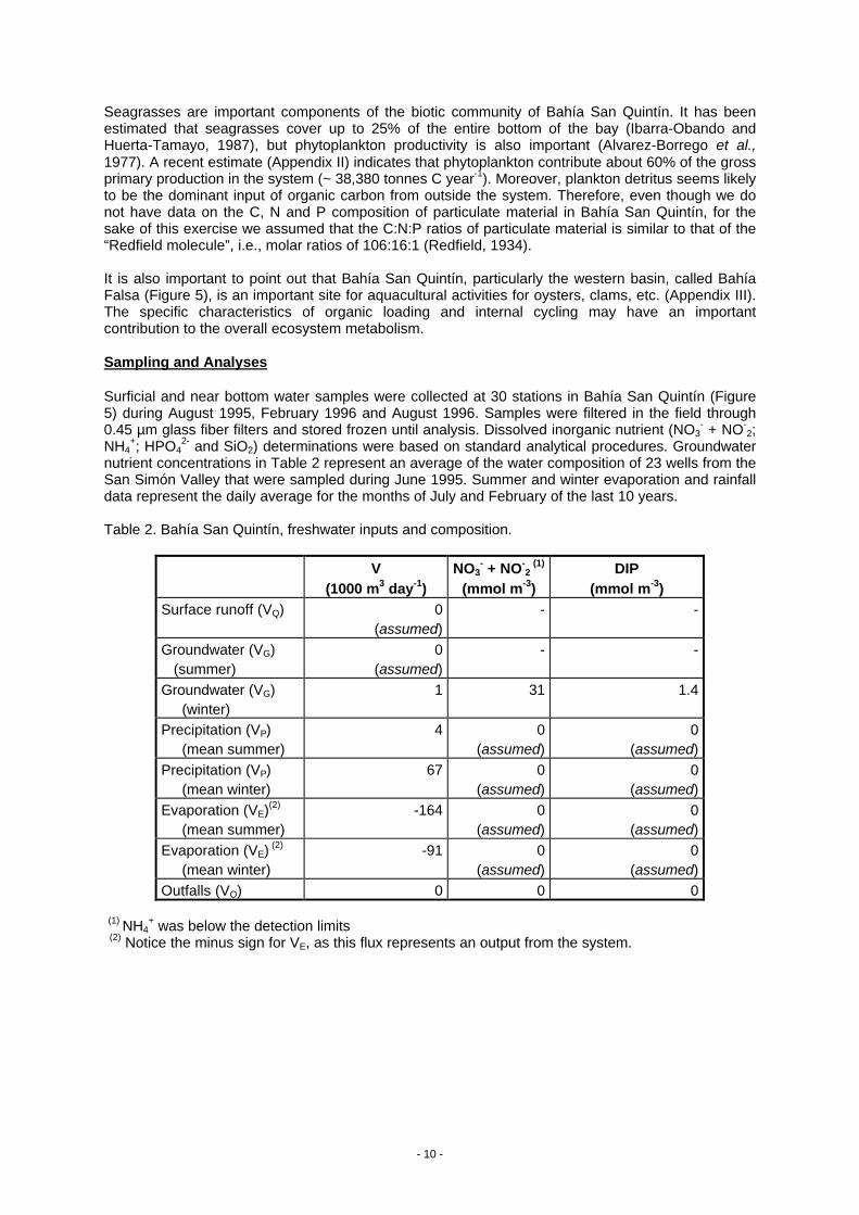
2- and SiO2) determinations were based on standard analytical procedures. Groundwaternutrient concentrations in Table 2 represent an average of the water composition of 23 wells from theSan Simón Valley that were sampled during June 1995. Summer and winter evaporation and rainfalldata represent the daily average for the months of July and February of the last 10 years.
Table 2. Bahía San Quintín, freshwater inputs and composition.
(1) NH4+ was below the detection limits
(2) Notice the minus sign for VE, as this flux represents an output from the system.
V(1000 m3 day-1)
NO3- + NO-
2 (1)
(mmol m-3)DIP
(mmol m-3)Surface runoff (VQ) 0
(assumed)- -
Groundwater (VG) (summer)
0(assumed)
- -
Groundwater (VG) (winter)
1 31 1.4
Precipitation (VP) (mean summer)
4 0(assumed)
0(assumed)
Precipitation (VP) (mean winter)
67 0(assumed)
0(assumed)
Evaporation (VE)(2)
(mean summer)-164 0
(assumed)0
(assumed)Evaporation (VE) (2)
(mean winter)-91 0
(assumed)0
(assumed)Outfalls (VO) 0 0 0
- 11 -
Water and Salt Budgets
From data in Table 2 we can calculate the water balance for each season from equation (5) (fromGordon et al., 1996):
dV1/dt = VQ + VP + VG + VO + VE + VR (5)
assuming steady state, i.e., dV1/dt = 0, then the residual volume (VR) is estimated
VR= -VQ - VP - VG - VO - VE (6)
Substituting terms in equation (6) with data in Table 2 we obtain a VR of
VR = -(0) - (4) - (0) - (0) - (-164) = +160 x103 m3 day-1
for summer (1995 and 1996) and,
VR = -(0) - (67) - (1) - (0) - (-91) = +23 x103 m3 day-1
for winter.
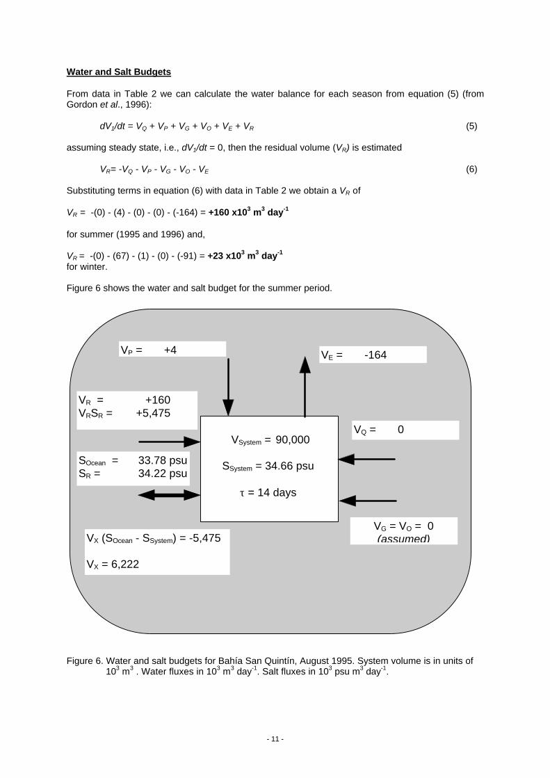
Figure 6 shows the water and salt budget for the summer period.
Figure 6. Water and salt budgets for Bahía San Quintín, August 1995. System volume is in units of103 m3 . Water fluxes in 103 m3 day-1. Salt fluxes in 103 psu m3 day-1.
VQ = 0
VE = -164VP = +4
VSystem = 90,000
SSystem = 34.66 psu
τ = 14 days
VR = +160VRSR = +5,475
SOcean = 33.78 psuSR = 34.22 psu
VX (SOcean - SSystem) = -5,475
VX = 6,222
VG = VO = 0(assumed)
- 12 -
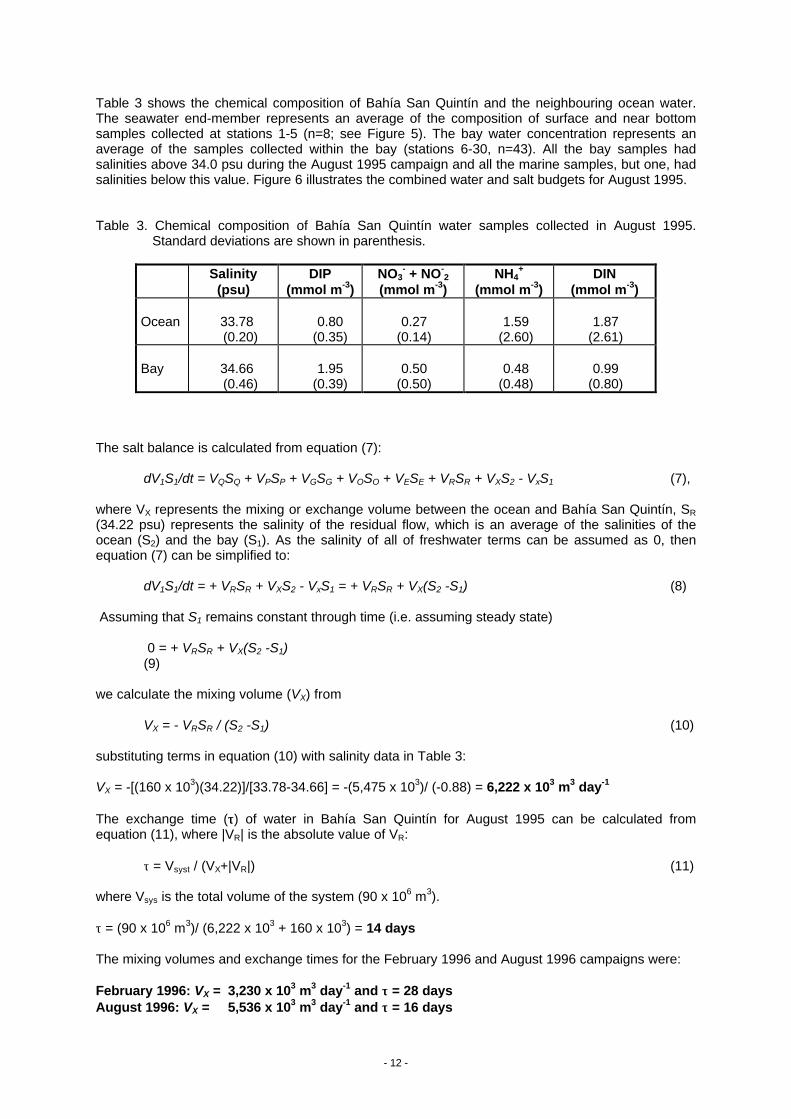
Table 3 shows the chemical composition of Bahía San Quintín and the neighbouring ocean water.The seawater end-member represents an average of the composition of surface and near bottomsamples collected at stations 1-5 (n=8; see Figure 5). The bay water concentration represents anaverage of the samples collected within the bay (stations 6-30, n=43). All the bay samples hadsalinities above 34.0 psu during the August 1995 campaign and all the marine samples, but one, hadsalinities below this value. Figure 6 illustrates the combined water and salt budgets for August 1995.
Table 3. Chemical composition of Bahía San Quintín water samples collected in August 1995.Standard deviations are shown in parenthesis.
The salt balance is calculated from equation (7):
dV1S1/dt = VQSQ + VPSP + VGSG + VOSO + VESE + VRSR + VXS2 - VxS1 (7),
where VX represents the mixing or exchange volume between the ocean and Bahía San Quintín, SR(34.22 psu) represents the salinity of the residual flow, which is an average of the salinities of theocean (S2) and the bay (S1). As the salinity of all of freshwater terms can be assumed as 0, thenequation (7) can be simplified to:
dV1S1/dt = + VRSR + VXS2 - VxS1 = + VRSR + VX(S2 -S1) (8)
Assuming that S1 remains constant through time (i.e. assuming steady state)
0 = + VRSR + VX(S2 -S1)(9)
we calculate the mixing volume (VX) from
VX = - VRSR / (S2 -S1) (10)
substituting terms in equation (10) with salinity data in Table 3:
VX = -[(160 x 103)(34.22)]/[33.78-34.66] = -(5,475 x 103)/ (-0.88) = 6,222 x 103 m3 day-1
The exchange time (ττ) of water in Bahía San Quintín for August 1995 can be calculated fromequation (11), where |VR| is the absolute value of VR:
τ = Vsyst / (VX+|VR|) (11)
where Vsys is the total volume of the system (90 x 106 m3).
τ = (90 x 106 m3)/ (6,222 x 103 + 160 x 103) = 14 days
The mixing volumes and exchange times for the February 1996 and August 1996 campaigns were:
February 1996: VX = 3,230 x 103 m3 day-1 and ττ = 28 daysAugust 1996: VX = 5,536 x 103 m3 day-1 and ττ = 16 days
Salinity(psu)
DIP(mmol m-3)
NO3- + NO-
2
(mmol m-3)NH4
+
(mmol m-3)DIN
(mmol m-3)
Ocean 33.78(0.20)
0.80(0.35)
0.27(0.14)
1.59(2.60)
1.87(2.61)
Bay 34.66(0.46)
1.95(0.39)
0.50(0.50)
0.48(0.48)
0.99(0.80)

- 13 -
Budgets of Nonconservative Materials
The balance of nonconservative materials is calculated from equation (12):
dV1Y1/dt = VQYQ + VPYP + VGYG + VOYO + VEYE + VRYR + VXY2 - VxY1 + ∆Y (12)
where ∆Y represents the net internal source or sink, that is, nonconservative flux, of element Y.
As groundwater is the only potentially important terrigenous source of Y in Bahía San Quintín (Table2), equation (12) can be reduced to:
dV1Y1/dt = + VGYG + VRYR + VX(Y2 - Y1) + ∆Y (13)
Again assuming steady state, the general equation for calculating nonconservative fluxes ofdissolved materials (without gaseous phase) is:
∆Y = - VGYG - VRYR - VX(Y2 - Y1) (14)
P BalanceThe nonconservative flux of P, ∆P, in Bahía San Quintín for the August 1995 campaign is calculatedfrom data in Tables 2 and 3 and illustrated in Figure 7:
∆P =-(0) - [(160 x 103)(1.38)] - [(6,222 x 103)(0.80-1.95)] = 6,934 x 103 mmol day-1 =+6,934 mol day-1
In order to establish comparisons with other systems, ∆P can be reported as a rate by normalising bythe area of the system (42 x 106 m2), thus,
∆∆P = +0.17 mmol m-2 day-1
∆P values for the other campaigns were:
February 1996: +586 mol day-1 (+0.01 mmol m-2 day-1)August 1996: +7,767 mol day-1 (+0.19 mmol m-2 day-1)
N BalanceSeparate budgets may be calculated for the different nitrogen species analysed in this study (NO3
- +NO-
2 and NH4+), however, we only show here the budget for the total dissolved inorganic nitrogen
(DIN) which is needed for looking at the stoichiometric linkages among nonconservative budgets andfor the estimation of N metabolism in the system.
The nonconservative flux of N, ∆N, in Bahía San Quintín for the August 1995 campaign is calculatedfrom data in Tables 2 and 3 and Figure 6, and illustrated in Figure 7:
∆N =-(0) - [(160 x 103)(1.43)] - [(6,222 x 103)(1.87-0.99)] = -5,704 x 103 mmol day-1= -5,704 mol day-
1
The ∆N normalised by the area of the system was,
∆∆N = -0.14 mmol m-2 day-1
∆N values for the other campaigns were:
February 1996: -21,906 mol day-1 (-0.52 mmol m-2 day-1)August 1996: +12,623 mol day-1 (+0.30 mmol m-2 day-1)

- 14 -
Figure 7. DIP and DIN budgets for Bahía San Quintín, August 1995. Fluxes in mol day-1.
DINSystem = 0.99 mmol m-3
∆DIN = -5,704
DINQ = 0 mmol m-3
VQ DINQ = 0
DINatm = 0(assumed)
VR DINR = +229
VX (DINOcean -DINSystem) = +5,475VG DING = VQ DINQ = 0
(assumed)
DINOcean=1.87mmol m-3
DINR = 1.43 mmol m-3
DIPQ = 0 mmol m-3
VQ DIPQ = 0
DIPatm = 0(assumed)
DIPSystem = 1.95 mmol m-3
∆DIP = +6,934
VR DIPR = +221
DIPOcean=0.80 mmol m-3
DIPR = 1.38 mmol m-3
VX (DIPOcean -DIPSystem) = -7,155 VG DIPG = VQ DIPQ = 0(assumed)
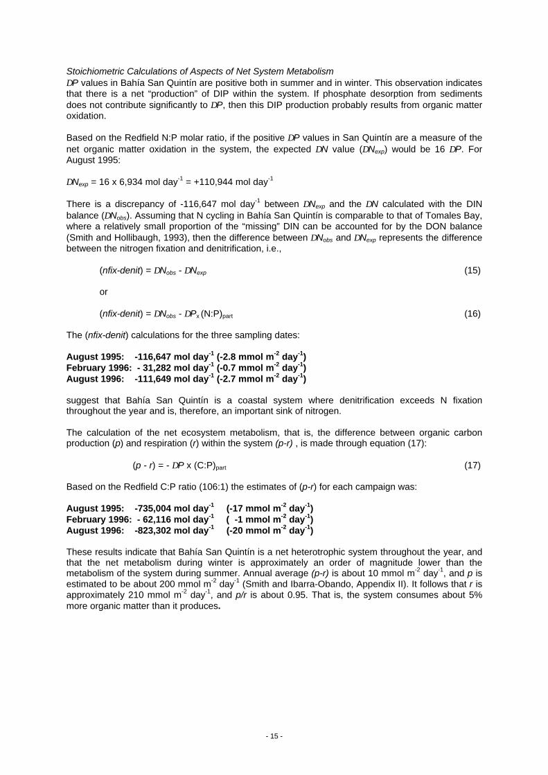
- 15 -
Stoichiometric Calculations of Aspects of Net System Metabolism∆P values in Bahía San Quintín are positive both in summer and in winter. This observation indicatesthat there is a net “production” of DIP within the system. If phosphate desorption from sedimentsdoes not contribute significantly to ∆P, then this DIP production probably results from organic matteroxidation.
Based on the Redfield N:P molar ratio, if the positive ∆P values in San Quintín are a measure of thenet organic matter oxidation in the system, the expected ∆N value (∆Nexp) would be 16 ∆P. ForAugust 1995:
∆Nexp = 16 x 6,934 mol day-1 = +110,944 mol day-1
There is a discrepancy of -116,647 mol day-1 between ∆Nexp and the ∆N calculated with the DINbalance (∆Nobs). Assuming that N cycling in Bahía San Quintín is comparable to that of Tomales Bay,where a relatively small proportion of the “missing” DIN can be accounted for by the DON balance(Smith and Hollibaugh, 1993), then the difference between ∆Nobs and ∆Nexp represents the differencebetween the nitrogen fixation and denitrification, i.e.,
(nfix-denit) = ∆Nobs - ∆Nexp (15)
or
(nfix-denit) = ∆Nobs - ∆Px (N:P)part (16)
The (nfix-denit) calculations for the three sampling dates:
August 1995: -116,647 mol day-1 (-2.8 mmol m-2 day-1)February 1996: - 31,282 mol day-1 (-0.7 mmol m-2 day-1)August 1996: -111,649 mol day-1 (-2.7 mmol m-2 day-1)
suggest that Bahía San Quintín is a coastal system where denitrification exceeds N fixationthroughout the year and is, therefore, an important sink of nitrogen.
The calculation of the net ecosystem metabolism, that is, the difference between organic carbonproduction (p) and respiration (r) within the system (p-r) , is made through equation (17):
(p - r) = - ∆P x (C:P)part (17)
Based on the Redfield C:P ratio (106:1) the estimates of (p-r) for each campaign was:
August 1995: -735,004 mol day-1 (-17 mmol m-2 day-1)February 1996: - 62,116 mol day-1 ( -1 mmol m-2 day-1)August 1996: -823,302 mol day-1 (-20 mmol m-2 day-1)
These results indicate that Bahía San Quintín is a net heterotrophic system throughout the year, andthat the net metabolism during winter is approximately an order of magnitude lower than themetabolism of the system during summer. Annual average (p-r) is about 10 mmol m-2 day-1, and p isestimated to be about 200 mmol m-2 day-1 (Smith and Ibarra-Obando, Appendix II). It follows that r isapproximately 210 mmol m-2 day-1, and p/r is about 0.95. That is, the system consumes about 5%more organic matter than it produces.
- 16 -
2.1.3) Bahía San Luis Gonzaga, Baja CaliforniaF. Delgadillo-Hinojosa and J. A. Segovia Zavala
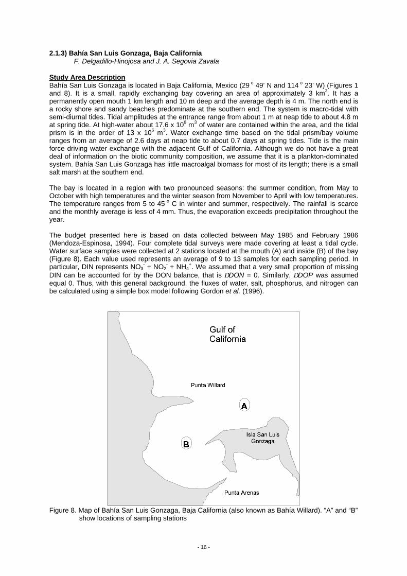
Study Area DescriptionBahía San Luis Gonzaga is located in Baja California, Mexico (29 o 49’ N and 114 o 23’ W) (Figures 1and 8). It is a small, rapidly exchanging bay covering an area of approximately 3 km2. It has apermanently open mouth 1 km length and 10 m deep and the average depth is 4 m. The north end isa rocky shore and sandy beaches predominate at the southern end. The system is macro-tidal withsemi-diurnal tides. Tidal amplitudes at the entrance range from about 1 m at neap tide to about 4.8 mat spring tide. At high-water about 17.6 x 10⁶ m3 of water are contained within the area, and the tidalprism is in the order of 13 x 106 m3. Water exchange time based on the tidal prism/bay volumeranges from an average of 2.6 days at neap tide to about 0.7 days at spring tides. Tide is the mainforce driving water exchange with the adjacent Gulf of California. Although we do not have a greatdeal of information on the biotic community composition, we assume that it is a plankton-dominatedsystem. Bahía San Luis Gonzaga has little macroalgal biomass for most of its length; there is a smallsalt marsh at the southern end.
The bay is located in a region with two pronounced seasons: the summer condition, from May toOctober with high temperatures and the winter season from November to April with low temperatures.The temperature ranges from 5 to 45 o C in winter and summer, respectively. The rainfall is scarceand the monthly average is less of 4 mm. Thus, the evaporation exceeds precipitation throughout theyear.
The budget presented here is based on data collected between May 1985 and February 1986(Mendoza-Espinosa, 1994). Four complete tidal surveys were made covering at least a tidal cycle.Water surface samples were collected at 2 stations located at the mouth (A) and inside (B) of the bay(Figure 8). Each value used represents an average of 9 to 13 samples for each sampling period. Inparticular, DIN represents NO3
- + NO2- + NH4
+. We assumed that a very small proportion of missingDIN can be accounted for by the DON balance, that is ∆DON = 0. Similarly, ∆DOP was assumedequal 0. Thus, with this general background, the fluxes of water, salt, phosphorus, and nitrogen canbe calculated using a simple box model following Gordon et al. (1996).
Figure 8. Map of Bahía San Luis Gonzaga, Baja California (also known as Bahía Willard). “A” and “B”show locations of sampling stations
- 17 -
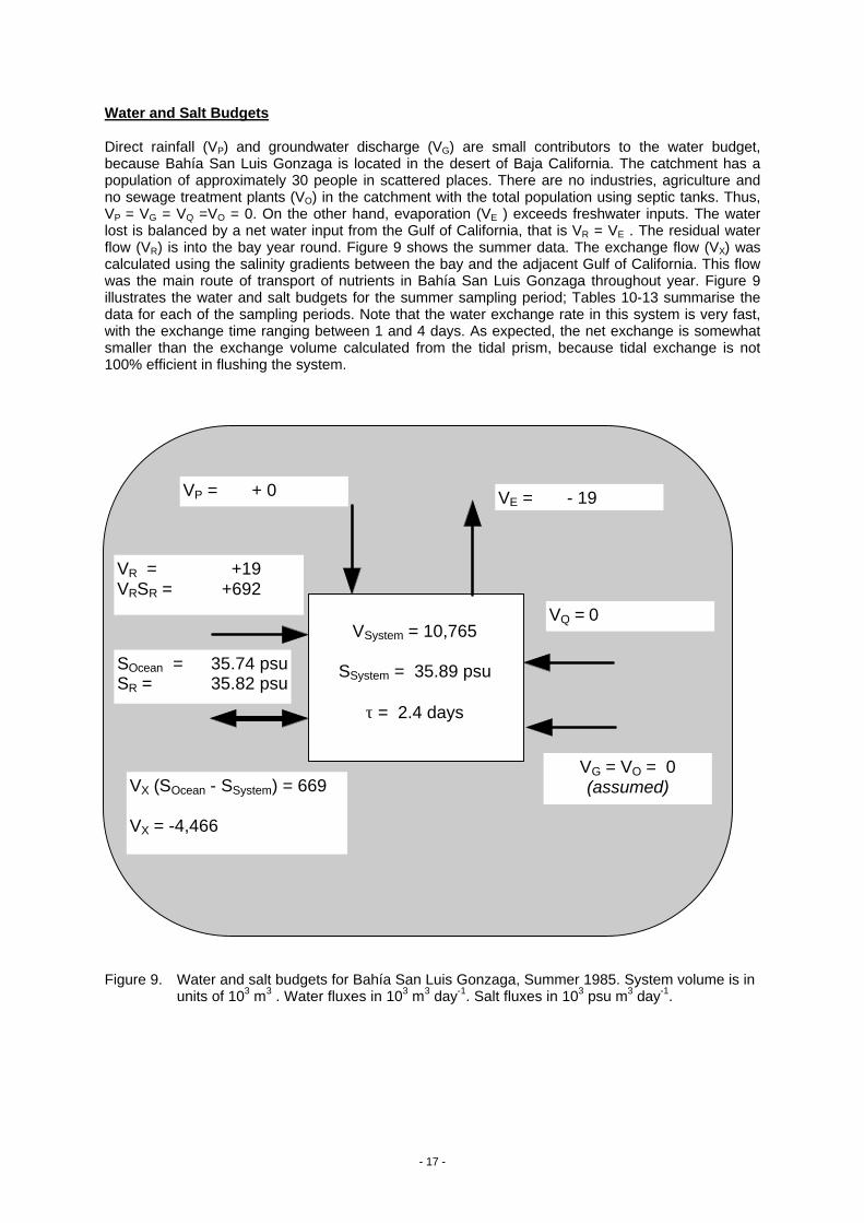
Water and Salt Budgets
Direct rainfall (VP) and groundwater discharge (VG) are small contributors to the water budget,because Bahía San Luis Gonzaga is located in the desert of Baja California. The catchment has apopulation of approximately 30 people in scattered places. There are no industries, agriculture andno sewage treatment plants (VO) in the catchment with the total population using septic tanks. Thus,VP = VG = VQ =VO = 0. On the other hand, evaporation (VE ) exceeds freshwater inputs. The waterlost is balanced by a net water input from the Gulf of California, that is VR = VE . The residual waterflow (VR) is into the bay year round. Figure 9 shows the summer data. The exchange flow (VX) wascalculated using the salinity gradients between the bay and the adjacent Gulf of California. This flowwas the main route of transport of nutrients in Bahía San Luis Gonzaga throughout year. Figure 9illustrates the water and salt budgets for the summer sampling period; Tables 10-13 summarise thedata for each of the sampling periods. Note that the water exchange rate in this system is very fast,with the exchange time ranging between 1 and 4 days. As expected, the net exchange is somewhatsmaller than the exchange volume calculated from the tidal prism, because tidal exchange is not100% efficient in flushing the system.
VQ = 0
VE = - 19VP = + 0
VSystem = 10,765
SSystem = 35.89 psu
τ = 2.4 days
VR = +19VRSR = +692
SOcean = 35.74 psuSR = 35.82 psu
VX (SOcean - SSystem) = 669
VX = -4,466
VG = VO = 0(assumed)
Figure 9. Water and salt budgets for Bahía San Luis Gonzaga, Summer 1985. System volume is inunits of 103 m3 . Water fluxes in 103 m3 day-1. Salt fluxes in 103 psu m3 day-1.
- 18 -
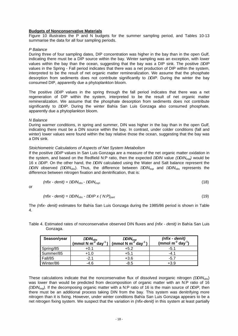
Budgets of Nonconservative MaterialsFigure 10 illustrates the P and N budgets for the summer sampling period, and Tables 10-13summarise the data for all four sampling periods.
P BalanceDuring three of four sampling dates, DIP concentration was higher in the bay than in the open Gulf,indicating there must be a DIP source within the bay. Winter sampling was an exception, with lowervalues within the bay than the ocean, suggesting that the bay was a DIP sink. The positive ∆DIPvalues in the Spring - Fall period indicates that there was a net production of DIP within the system,interpreted to be the result of net organic matter remineralization. We assume that the phosphatedesorption from sediments does not contribute significantly to ∆DIP. During the winter the bayconsumed DIP, apparently due a phytoplankton bloom.
The positive ∆DIP values in the spring through the fall period indicates that there was a netregeneration of DIP within the system, interpreted to be the result of net organic matterremineralization. We assume that the phosphate desorption from sediments does not contributesignificantly to ∆DIP. During the winter Bahía San Luis Gonzaga also consumed phosphate,apparently due a phytoplankton bloom.
N BalanceDuring warmer conditions, in spring and summer, DIN was higher in the bay than in the open Gulf,indicating there must be a DIN source within the bay. In contrast, under colder conditions (fall andwinter) lower values were found within the bay relative those the ocean, suggesting that the bay wasa DIN sink.
Stoichiometric Calculations of Aspects of Net System MetabolismIf the positive ∆DIP values in San Luis Gonzaga are a measure of the net organic matter oxidation inthe system, and based on the Redfield N:P ratio, then the expected ∆DIN value (∆DINexp) would be16 x ∆DIP. On the other hand, the ∆DIN calculated using the Water and Salt balance represent the∆DIN observed (∆DINobs). Thus, the difference between ∆DINexp and ∆DINobs represents thedifference between nitrogen fixation and denitrification, that is:
(nfix - denit) = ∆DINobs - ∆DINexp\ (18)or
(nfix - denit) = ∆DINobs - ∆DIP x ( N:P)part (19)
The (nfix- denit) estimates for Bahía San Luis Gonzaga during the 1985/86 period is shown in Table4.
Table 4. Estimated rates of nonconservative observed DIN fluxes and (nfix - denit) in Bahía San LuisGonzaga.
These calculations indicate that the nonconservative flux of dissolved inorganic nitrogen (∆DINobs)was lower than would be predicted from decomposition of organic matter with an N:P ratio of 16(∆DINexp). If the decomposing organic matter with a N:P ratio of 16 is the main source of ∆DIP, thenthere must be an additional process taking DIN from the bay. This system was denitrifying morenitrogen than it is fixing. However, under winter conditions Bahía San Luis Gonzaga appears to be anet nitrogen fixing system. We suspect that the variation in (nfix-denit) in this system at least partially
Season/year ∆∆DINobs
(mmol N m-2 day-1 )∆∆DINexp
(mmol N m-2 day-1 )(nfix - denit)
(mmol m-2 day-1)Spring/85 +0.1 +5.2 -5.1Summer/85 +1.0 +5.1 -4.1Fall/85 -2.1 +3.6 -5.7Winter/86 -4.6 -8.5 +3.9
- 19 -
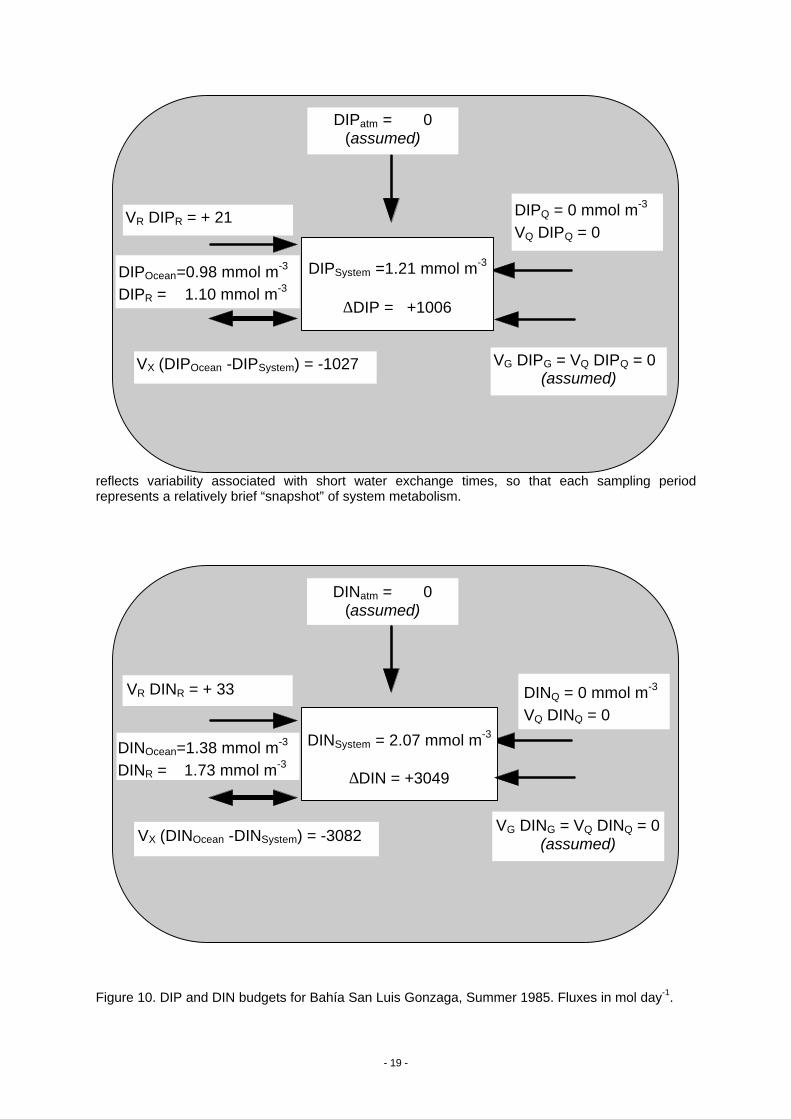
reflects variability associated with short water exchange times, so that each sampling periodrepresents a relatively brief “snapshot” of system metabolism.
Figure 10. DIP and DIN budgets for Bahía San Luis Gonzaga, Summer 1985. Fluxes in mol day-1.
DIPQ = 0 mmol m-3
VQ DIPQ = 0
DIPatm = 0(assumed)
DIPSystem =1.21 mmol m-3
∆DIP = +1006
VR DIPR = + 21
DIPOcean=0.98 mmol m-3
DIPR = 1.10 mmol m-3
VX (DIPOcean -DIPSystem) = -1027 VG DIPG = VQ DIPQ = 0(assumed)
DINQ = 0 mmol m-3
VQ DINQ = 0
DINatm = 0(assumed)
DINSystem = 2.07 mmol m-3
∆DIN = +3049
VR DINR = + 33
VX (DINOcean -DINSystem) = -3082VG DING = VQ DINQ = 0
(assumed)
DINOcean=1.38 mmol m-3
DINR = 1.73 mmol m-3
- 20 -
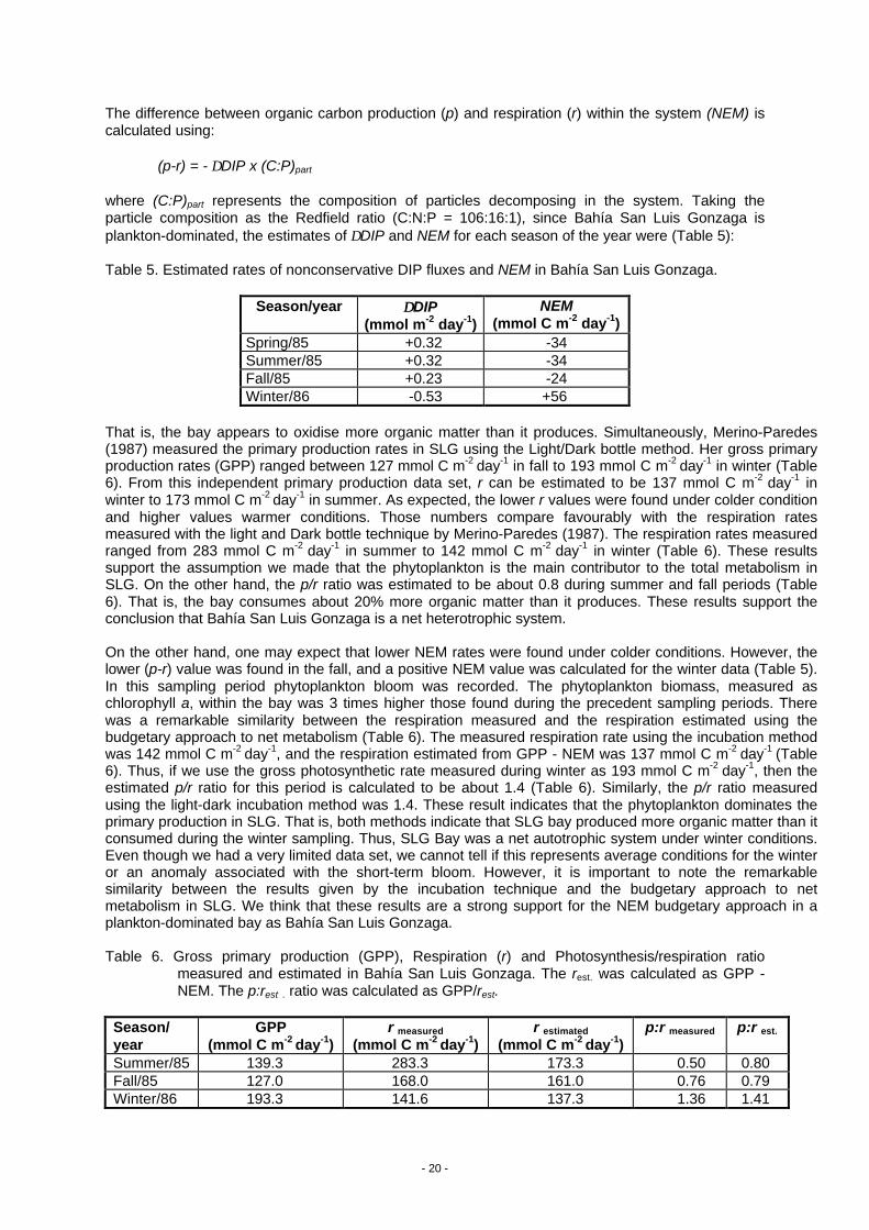
The difference between organic carbon production (p) and respiration (r) within the system (NEM) iscalculated using:
(p-r) = - ∆DIP x (C:P)part
where (C:P)part represents the composition of particles decomposing in the system. Taking theparticle composition as the Redfield ratio (C:N:P = 106:16:1), since Bahía San Luis Gonzaga isplankton-dominated, the estimates of ∆DIP and NEM for each season of the year were (Table 5):
Table 5. Estimated rates of nonconservative DIP fluxes and NEM in Bahía San Luis Gonzaga.
That is, the bay appears to oxidise more organic matter than it produces. Simultaneously, Merino-Paredes(1987) measured the primary production rates in SLG using the Light/Dark bottle method. Her gross primaryproduction rates (GPP) ranged between 127 mmol C m-2 day-1 in fall to 193 mmol C m-2 day-1 in winter (Table6). From this independent primary production data set, r can be estimated to be 137 mmol C m-2 day-1 inwinter to 173 mmol C m-2 day-1 in summer. As expected, the lower r values were found under colder conditionand higher values warmer conditions. Those numbers compare favourably with the respiration ratesmeasured with the light and Dark bottle technique by Merino-Paredes (1987). The respiration rates measuredranged from 283 mmol C m-2 day-1 in summer to 142 mmol C m-2 day-1 in winter (Table 6). These resultssupport the assumption we made that the phytoplankton is the main contributor to the total metabolism inSLG. On the other hand, the p/r ratio was estimated to be about 0.8 during summer and fall periods (Table6). That is, the bay consumes about 20% more organic matter than it produces. These results support theconclusion that Bahía San Luis Gonzaga is a net heterotrophic system.
On the other hand, one may expect that lower NEM rates were found under colder conditions. However, thelower (p-r) value was found in the fall, and a positive NEM value was calculated for the winter data (Table 5).In this sampling period phytoplankton bloom was recorded. The phytoplankton biomass, measured aschlorophyll a, within the bay was 3 times higher those found during the precedent sampling periods. Therewas a remarkable similarity between the respiration measured and the respiration estimated using thebudgetary approach to net metabolism (Table 6). The measured respiration rate using the incubation methodwas 142 mmol C m-2 day-1, and the respiration estimated from GPP - NEM was 137 mmol C m-2 day-1 (Table6). Thus, if we use the gross photosynthetic rate measured during winter as 193 mmol C m-2 day-1, then theestimated p/r ratio for this period is calculated to be about 1.4 (Table 6). Similarly, the p/r ratio measuredusing the light-dark incubation method was 1.4. These result indicates that the phytoplankton dominates theprimary production in SLG. That is, both methods indicate that SLG bay produced more organic matter than itconsumed during the winter sampling. Thus, SLG Bay was a net autotrophic system under winter conditions.Even though we had a very limited data set, we cannot tell if this represents average conditions for the winteror an anomaly associated with the short-term bloom. However, it is important to note the remarkablesimilarity between the results given by the incubation technique and the budgetary approach to netmetabolism in SLG. We think that these results are a strong support for the NEM budgetary approach in aplankton-dominated bay as Bahía San Luis Gonzaga.
Table 6. Gross primary production (GPP), Respiration (r) and Photosynthesis/respiration ratiomeasured and estimated in Bahía San Luis Gonzaga. The rest. was calculated as GPP -NEM. The p:rest . ratio was calculated as GPP/rest.
Season/year
GPP(mmol C m-2 day-1)
r measured
(mmol C m-2 day-1)r estimated
(mmol C m-2 day-1)p:r measured p:r est.
Summer/85 139.3 283.3 173.3 0.50 0.80Fall/85 127.0 168.0 161.0 0.76 0.79Winter/86 193.3 141.6 137.3 1.36 1.41
Season/year ∆∆DIP(mmol m-2 day-1)
NEM(mmol C m-2 day-1)
Spring/85 +0.32 -34Summer/85 +0.32 -34Fall/85 +0.23 -24Winter/86 -0.53 +56
- 21 -
2.1.4) Estero La Cruz, SonoraM. Botello-Ruvalcaba and E. Valdez-Holguín
Study Area DescriptionLa Cruz is a characteristic desert coastal lagoon from the north-west of Mexico. In lagoonal systemswithin this region the evaporation is an order of magnitude higher than freshwater input fromprecipitation. Also, groundwater is characterised by saline intrusion, and the circulation is mainlydetermined by tide and wind induced forces (Botello-Ruvalcaba and Valdez-Holguín, 1990; Valdez-Holguín, 1994). In addition, these systems represent the northern frontier for some mangrove speciessuch as Avicenia germinais and Rhizophora mangle in the American pacific coast (Castro-Longoria etal., 1989)
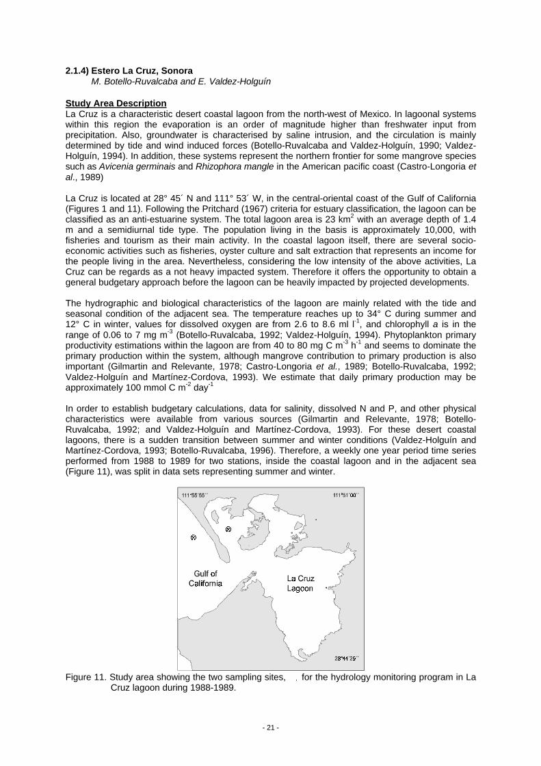
La Cruz is located at 28° 45´ N and 111° 53´ W, in the central-oriental coast of the Gulf of California(Figures 1 and 11). Following the Pritchard (1967) criteria for estuary classification, the lagoon can beclassified as an anti-estuarine system. The total lagoon area is 23 km2 with an average depth of 1.4m and a semidiurnal tide type. The population living in the basis is approximately 10,000, withfisheries and tourism as their main activity. In the coastal lagoon itself, there are several socio-economic activities such as fisheries, oyster culture and salt extraction that represents an income forthe people living in the area. Nevertheless, considering the low intensity of the above activities, LaCruz can be regards as a not heavy impacted system. Therefore it offers the opportunity to obtain ageneral budgetary approach before the lagoon can be heavily impacted by projected developments.
The hydrographic and biological characteristics of the lagoon are mainly related with the tide andseasonal condition of the adjacent sea. The temperature reaches up to 34° C during summer and12° C in winter, values for dissolved oxygen are from 2.6 to 8.6 ml l-1, and chlorophyll a is in therange of 0.06 to 7 mg m-3 (Botello-Ruvalcaba, 1992; Valdez-Holguín, 1994). Phytoplankton primaryproductivity estimations within the lagoon are from 40 to 80 mg C m-3 h-1 and seems to dominate theprimary production within the system, although mangrove contribution to primary production is alsoimportant (Gilmartin and Relevante, 1978; Castro-Longoria et al., 1989; Botello-Ruvalcaba, 1992;Valdez-Holguín and Martínez-Cordova, 1993). We estimate that daily primary production may beapproximately 100 mmol C m-2 day-1
In order to establish budgetary calculations, data for salinity, dissolved N and P, and other physicalcharacteristics were available from various sources (Gilmartin and Relevante, 1978; Botello-Ruvalcaba, 1992; and Valdez-Holguín and Martínez-Cordova, 1993). For these desert coastallagoons, there is a sudden transition between summer and winter conditions (Valdez-Holguín andMartínez-Cordova, 1993; Botello-Ruvalcaba, 1996). Therefore, a weekly one year period time seriesperformed from 1988 to 1989 for two stations, inside the coastal lagoon and in the adjacent sea(Figure 11), was split in data sets representing summer and winter.
Figure 11. Study area showing the two sampling sites, ⊗⊗, for the hydrology monitoring program in LaCruz lagoon during 1988-1989.

- 22 -
Water and Salt Budgets
Figure 12 summarises the water and salt budgets for the summer, and Tables 10-13 include both thesummer and winter data. La Cruz basin has problems with saline intrusion into the groundwater, sogroundwater input (VG) can be considered to be 0. River inflow (VQ) is also 0. Precipitation is highlyseasonal and very low. Finally, evaporation dominates the freshwater budget throughout the year,resulting in high salinity values within the system, which can be up to 4 psu above that of theadjacent sea. The water exchange time was 21 days in the summer and 43 days in the winter.
Figure 12. Water and salt budgets for Estero La Cruz, Summer. System volume is in units of 103 m3.Water fluxes in 103 m3 day-1. Salt fluxes in 103 psu m3 day-1.
VQ = 0
VE = - 151VP = + 15
VSystem = 32,000
SSystem = 39.40 psu
τ = 21 days
VR = +136VRSR = +5,111
SOcean = 35.75 psuSR = 37.58 psu
VX (SOcean - SSystem) = -5,111
VX = + 1,400
VG = VO = 0(assumed)
- 23 -
Budgets of Nonconservative Materials
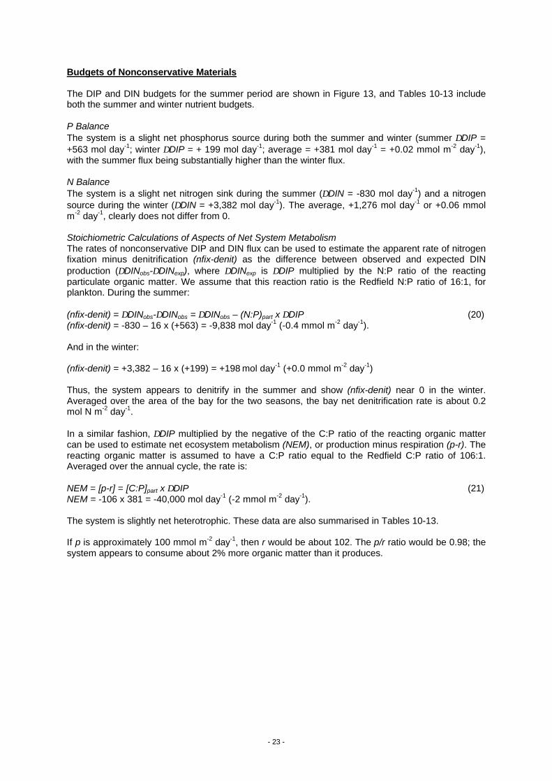
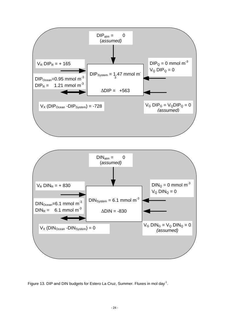
The DIP and DIN budgets for the summer period are shown in Figure 13, and Tables 10-13 includeboth the summer and winter nutrient budgets.
P BalanceThe system is a slight net phosphorus source during both the summer and winter (summer ∆DIP =+563 mol day-1; winter ∆DIP = + 199 mol day-1; average = +381 mol day-1 = +0.02 mmol m-2 day-1),with the summer flux being substantially higher than the winter flux.
N BalanceThe system is a slight net nitrogen sink during the summer (∆DIN = -830 mol day-1) and a nitrogensource during the winter (∆DIN = +3,382 mol day-1). The average, +1,276 mol day-1 or +0.06 mmolm-2 day-1, clearly does not differ from 0.
Stoichiometric Calculations of Aspects of Net System MetabolismThe rates of nonconservative DIP and DIN flux can be used to estimate the apparent rate of nitrogenfixation minus denitrification (nfix-denit) as the difference between observed and expected DINproduction (∆DINobs-∆DINexp), where ∆DINexp is ∆DIP multiplied by the N:P ratio of the reactingparticulate organic matter. We assume that this reaction ratio is the Redfield N:P ratio of 16:1, forplankton. During the summer:
(nfix-denit) = ∆DINobs-∆DINobs = ∆DINobs – (N:P)part x ∆DIP (20)(nfix-denit) = -830 – 16 x (+563) = -9,838 mol day-1 (-0.4 mmol m-2 day-1).
And in the winter:
(nfix-denit) = +3,382 – 16 x (+199) = +198 mol day-1 (+0.0 mmol m-2 day-1)
Thus, the system appears to denitrify in the summer and show (nfix-denit) near 0 in the winter.Averaged over the area of the bay for the two seasons, the bay net denitrification rate is about 0.2mol N m-2 day-1.
In a similar fashion, ∆DIP multiplied by the negative of the C:P ratio of the reacting organic mattercan be used to estimate net ecosystem metabolism (NEM), or production minus respiration (p-r). Thereacting organic matter is assumed to have a C:P ratio equal to the Redfield C:P ratio of 106:1.Averaged over the annual cycle, the rate is:
NEM = [p-r] = [C:P]part x ∆DIP (21)NEM = -106 x 381 = -40,000 mol day-1 (-2 mmol m-2 day-1).
The system is slightly net heterotrophic. These data are also summarised in Tables 10-13.
If p is approximately 100 mmol m-2 day-1, then r would be about 102. The p/r ratio would be 0.98; thesystem appears to consume about 2% more organic matter than it produces.
- 24 -
Figure 13. DIP and DIN budgets for Estero La Cruz, Summer. Fluxes in mol day-1.
DINQ = 0 mmol m-3
VQ DINQ = 0
DINatm = 0(assumed)
DINSystem = 6.1 mmol m-3
∆DIN = -830
VR DINR = + 830
VX (DINOcean -DINSystem) = 0VG DING = VQ DINQ = 0
(assumed)
DINOcean=6.1 mmol m-3
DINR = 6.1 mmol m-3
DIPQ = 0 mmol m-3
VQ DIPQ = 0
DIPatm = 0(assumed)
DIPSystem = 1.47 mmol m-
3
∆DIP = +563
VR DIPR = + 165
DIPOcean=0.95 mmol m-3
DIPR = 1.21 mmol m-3
VX (DIPOcean -DIPSystem) = -728 VG DIPG = VQDIPQ = 0(assumed)
- 25 -
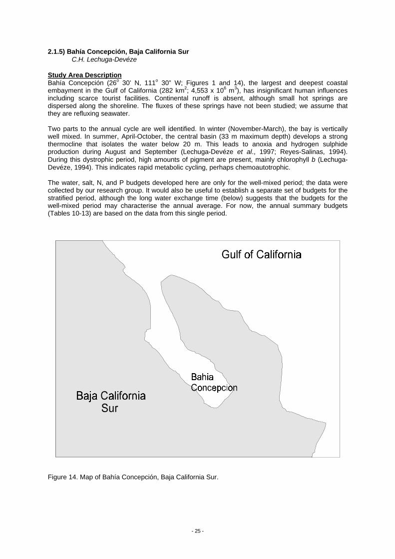
2.1.5) Bahía Concepción, Baja California SurC.H. Lechuga-Devéze
Study Area DescriptionBahía Concepción (26o 30’ N, 111o 30” W; Figures 1 and 14), the largest and deepest coastalembayment in the Gulf of California (282 km2; 4,553 x 106 m3), has insignificant human influencesincluding scarce tourist facilities. Continental runoff is absent, although small hot springs aredispersed along the shoreline. The fluxes of these springs have not been studied; we assume thatthey are refluxing seawater.
Two parts to the annual cycle are well identified. In winter (November-March), the bay is verticallywell mixed. In summer, April-October, the central basin (33 m maximum depth) develops a strongthermocline that isolates the water below 20 m. This leads to anoxia and hydrogen sulphideproduction during August and September (Lechuga-Devéze et al., 1997; Reyes-Salinas, 1994).During this dystrophic period, high amounts of pigment are present, mainly chlorophyll b (Lechuga-Devéze, 1994). This indicates rapid metabolic cycling, perhaps chemoautotrophic.
The water, salt, N, and P budgets developed here are only for the well-mixed period; the data werecollected by our research group. It would also be useful to establish a separate set of budgets for thestratified period, although the long water exchange time (below) suggests that the budgets for thewell-mixed period may characterise the annual average. For now, the annual summary budgets(Tables 10-13) are based on the data from this single period.
Figure 14. Map of Bahía Concepción, Baja California Sur.
- 26 -
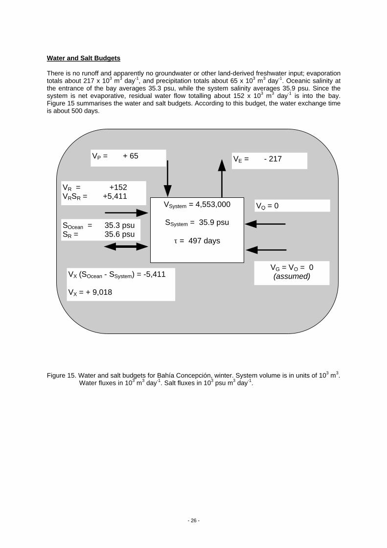
Water and Salt Budgets
There is no runoff and apparently no groundwater or other land-derived freshwater input; evaporationtotals about 217 x 103 m3 day-1, and precipitation totals about 65 x 103 m3 day-1. Oceanic salinity atthe entrance of the bay averages 35.3 psu, while the system salinity averages 35.9 psu. Since thesystem is net evaporative, residual water flow totalling about 152 x 103 m3 day-1 is into the bay.Figure 15 summarises the water and salt budgets. According to this budget, the water exchange timeis about 500 days.
Figure 15. Water and salt budgets for Bahía Concepción, winter. System volume is in units of 103 m3.Water fluxes in 103 m3 day-1. Salt fluxes in 103 psu m3 day-1.
VQ = 0
VE = - 217VP = + 65
VSystem = 4,553,000
SSystem = 35.9 psu
τ = 497 days
VR = +152VRSR = +5,411
SOcean = 35.3 psuSR = 35.6 psu
VX (SOcean - SSystem) = -5,411
VX = + 9,018
VG = VO = 0(assumed)
- 27 -
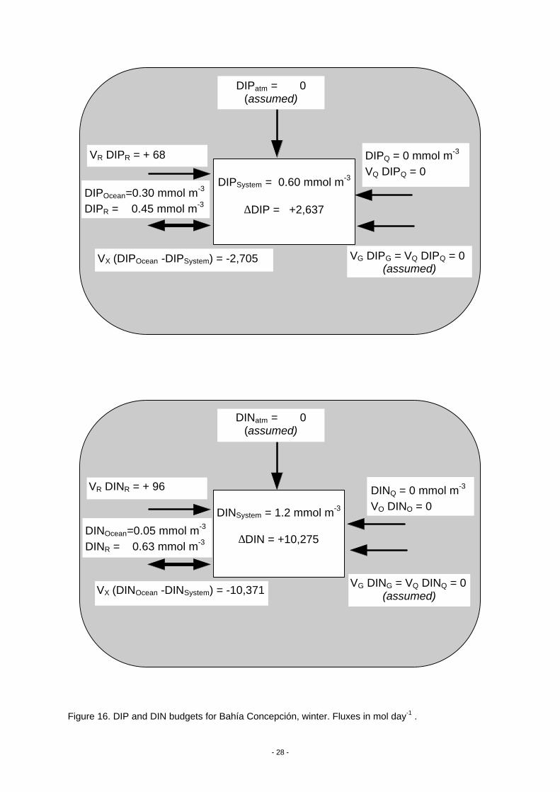
Budgets of Nonconservative Materials
P Balance
Figure 16 illustrates the P and N budgets for this system The mixing outflow of DIP from this systemis substantially larger than the residual inflow and demonstrates that there must be DIP production(∆DIP) of approximately +2,637 mol day-1 in the system. We assume that this representsdecomposition of organic matter. Because of the long water residence time, we assume that thisdecomposition rate is averaged over a period longer than one year.
N Balance
Similarly, the system shows strong net export of DIN (+10,371 mol day-1; Figure 16). Again, thisoutward mixing represents DIN production (∆DIN) and is assumed to represent decomposition oforganic matter.
Stoichiometric Calculations of Aspects of Net System Metabolism
The rates of DIP and DIN production can be used to estimate the apparent rate of nitrogen fixationminus denitrification (nfix-denit) as the difference between observed and expected DIN production(∆DINobs-∆DINexp), where ∆DINexp is ∆DIP multiplied by the N:P ratio of the reacting particulateorganic matter. We assume that this reaction ratio is the Redfield N:P ratio of 16:1, for plankton.Thus:
(nfix-denit) = ∆DINobs-∆DINobs = ∆DINobs – (N:P)part x ∆DIP (22)
(nfix-denit) = +10,276 – 16 x (+2,637) = -31,916 mol day-1
Averaged over the area of the bay, (nfix-denit) equals -0.1 mmol N m-2 day-1. This system appears tobe denitrifying at a relatively slow rate, although the nonconservative flux signal for DIN integratedover longer than a year is a strong signal.
In a similar fashion, ∆DIP multiplied by the negative of the C:P ratio of the reacting organic mattercan be used to estimate net ecosystem metabolism (NEM), or production minus respiration (p-r). Thereacting organic matter is assumed to have a C:P ratio equal to the Redfield C:P ratio of 106:1:
NEM = [p-r] = [C:P]part x ∆DIP (23)
NEM = -106 x 2,637 = -279,522 mol day-1.
Over the bay area, NEM equals –1 mmol m-2 day-1; that is, the system is slightly net heterotrophic.These data are also summarised in Tables 10-13.
- 28 -
Figure 16. DIP and DIN budgets for Bahía Concepción, winter. Fluxes in mol day-1 .
DIPQ = 0 mmol m-3
VQ DIPQ = 0
DIPatm = 0(assumed)
DIPSystem = 0.60 mmol m-3
∆DIP = +2,637
VR DIPR = + 68
DIPOcean=0.30 mmol m-3
DIPR = 0.45 mmol m-3
VX (DIPOcean -DIPSystem) = -2,705 VG DIPG = VQ DIPQ = 0(assumed)
DINQ = 0 mmol m-3
VQ DINQ = 0
DINatm = 0(assumed)
DINSystem = 1.2 mmol m-3
∆DIN = +10,275
VR DINR = + 96
VX (DINOcean -DINSystem) = -10,371VG DING = VQ DINQ = 0
(assumed)
DINOcean=0.05 mmol m-3
DINR = 0.63 mmol m-3
- 29 -
2.1.6) Ensenada de La Paz, Baja California SurC.H. Lechuga-Devéze
Study Area Description
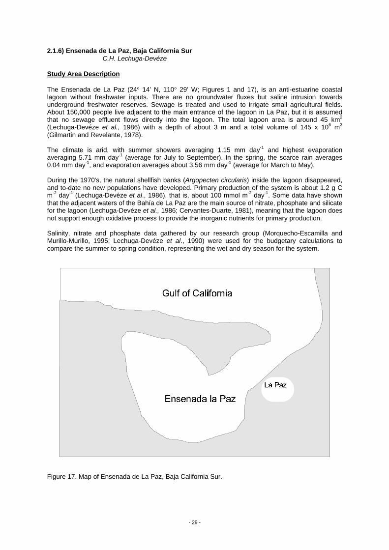
The Ensenada de La Paz (24° 14’ N, 110° 29’ W; Figures 1 and 17), is an anti-estuarine coastallagoon without freshwater inputs. There are no groundwater fluxes but saline intrusion towardsunderground freshwater reserves. Sewage is treated and used to irrigate small agricultural fields.About 150,000 people live adjacent to the main entrance of the lagoon in La Paz, but it is assumedthat no sewage effluent flows directly into the lagoon. The total lagoon area is around 45 km2
(Lechuga-Devéze et al., 1986) with a depth of about 3 m and a total volume of 145 x 106 m3
(Gilmartin and Revelante, 1978).
The climate is arid, with summer showers averaging 1.15 mm day-1 and highest evaporationaveraging 5.71 mm day-1 (average for July to September). In the spring, the scarce rain averages0.04 mm day-1, and evaporation averages about 3.56 mm day-1 (average for March to May).
During the 1970's, the natural shellfish banks (Argopecten circularis) inside the lagoon disappeared,and to-date no new populations have developed. Primary production of the system is about 1.2 g Cm-2 day-1 (Lechuga-Devéze et al., 1986), that is, about 100 mmol m-2 day-1. Some data have shownthat the adjacent waters of the Bahía de La Paz are the main source of nitrate, phosphate and silicatefor the lagoon (Lechuga-Devéze et al., 1986; Cervantes-Duarte, 1981), meaning that the lagoon doesnot support enough oxidative process to provide the inorganic nutrients for primary production.
Salinity, nitrate and phosphate data gathered by our research group (Morquecho-Escamilla andMurillo-Murillo, 1995; Lechuga-Devéze et al., 1990) were used for the budgetary calculations tocompare the summer to spring condition, representing the wet and dry season for the system.
Figure 17. Map of Ensenada de La Paz, Baja California Sur.
- 30 -
Water and Salt Budgets
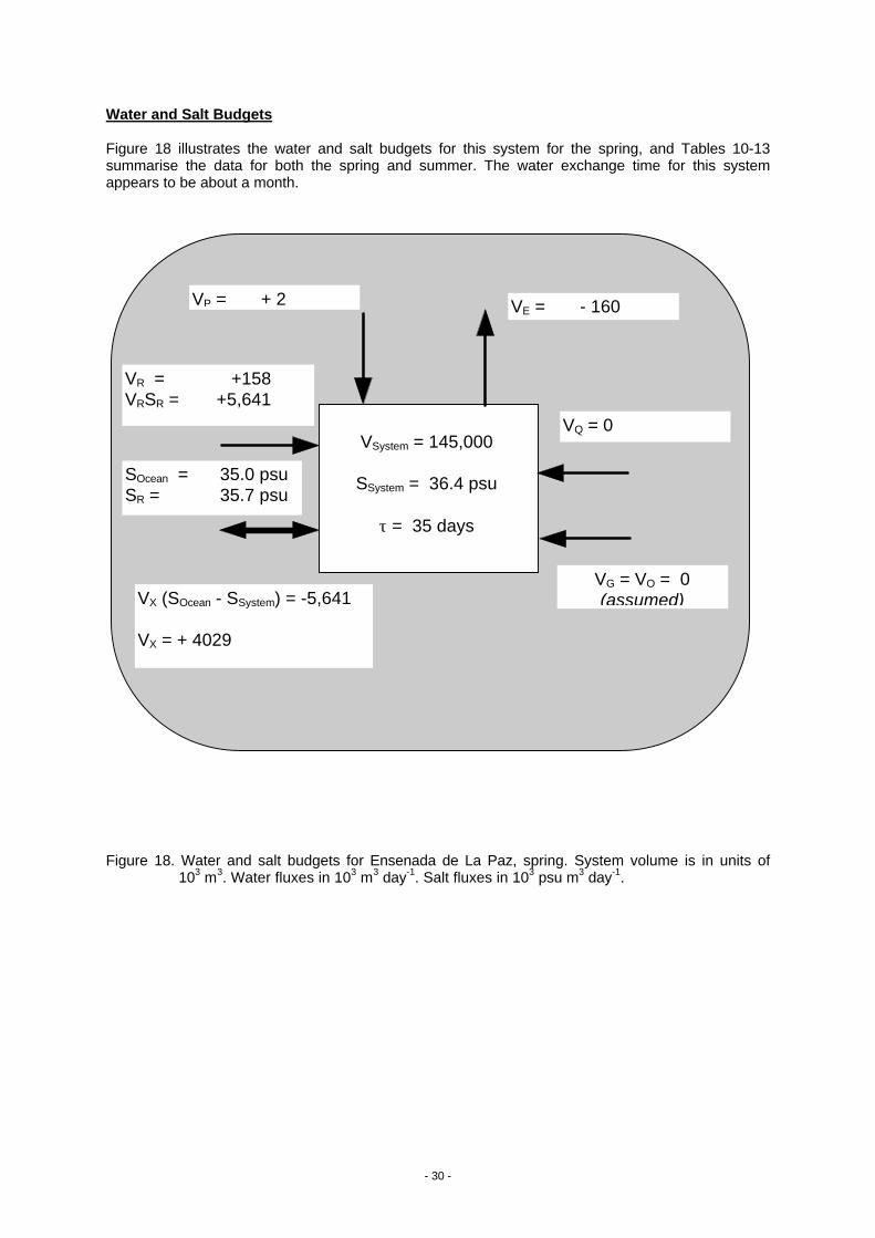
Figure 18 illustrates the water and salt budgets for this system for the spring, and Tables 10-13summarise the data for both the spring and summer. The water exchange time for this systemappears to be about a month.
Figure 18. Water and salt budgets for Ensenada de La Paz, spring. System volume is in units of103 m3. Water fluxes in 103 m3 day-1. Salt fluxes in 103 psu m3 day-1.
VQ = 0
VE = - 160VP = + 2
VSystem = 145,000
SSystem = 36.4 psu
τ = 35 days
VR = +158VRSR = +5,641
SOcean = 35.0 psuSR = 35.7 psu
VX (SOcean - SSystem) = -5,641
VX = + 4029
VG = VO = 0(assumed)
- 31 -
Budgets of Nonconservative Materials
P Balance
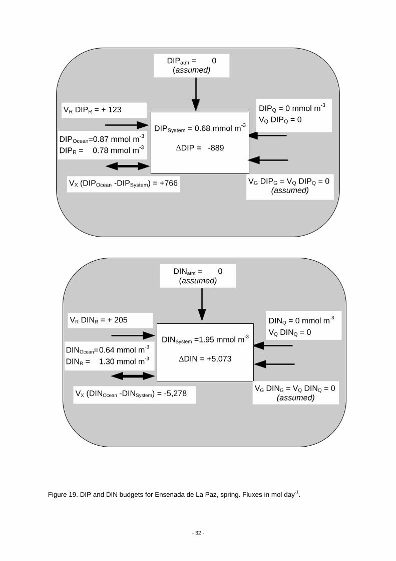
Figure 19 illustrates the P and N budgets for the spring, and Tables 10-13 summarise the data forboth spring and summer. With particular respect to ∆DIP, there appears to be substantial variation;DIP uptake occurs and is higher during the summer than the spring. The average ∆DIP of the twosampling periods is –1,914 mol day-1. Thus the system appears to be a net sink for DIP, mostlyderived from the ocean.
N Balance
The bay appears to be a net DIN source during the spring and about neutral with respect to DINduring the summer. The average ∆DIN of the two sampling periods is +2,706 mol day-1.
Stoichiometric Calculations of Aspects of Net System Metabolism
Nitrogen fixation minus denitrification (nfix-denit) is calculated from the difference between observedand expected ∆DIN, where the expected ∆DIN is calculated as 16 x ∆DIP. It is assumed that themajor sink for DIP is plankton. Table 7 illustrates these calculations for Ensenada de La Paz. Thesystem appears to fix nitrogen in excess of denitrification, by a rate averaging about 0.8 mmol m-2
day-1.
Table 7. Estimated rates of nonconservative observed DIN fluxes and (nfix - denit) in Ensenada deLa Paz.
The difference between organic carbon production, p, and respiration, r, within the system (NEM) iscalculated using:
(p-r) = - ∆P x ( C:P)part (23)
where (C:P)part represents the composition of particles reacting in the system. Taking the particlecomposition as the Redfield ratio (C:N:P = 106:16:1), since Ensenada de La Paz is assumed to be aplankton-dominated system, the estimates of ∆P and NEM are shown in Table 8:
Table 8. Estimated rates of nonconservative DIP fluxes and NEM in Ensenada de La Paz.
This system appears to be net autotrophic by approximately 5 mmol m-2 day-1.
Primary production has been estimated to be about 100 mmol m-2 day-1, implying that respiration isabout 95 and that the p/r ratio is about 1.05. This system appears to produce about 5% more organiccarbon that it consumes.
Season ∆∆DINobs
(mmol N m-2 day-1 )∆∆DINexp
(mmol N m-2 day-1 )(nfix – denit)
(mmol m-2 day-1)Spring +0.11 -0.32 +0.4Summer -0.01 +1.10 +1.1
Season ∆∆P (mmol m-2 day-1)
NEM(mmol C m-2 day-1)
Spring -0.02 +2Summer -0.07 +7
- 32 -
Figure 19. DIP and DIN budgets for Ensenada de La Paz, spring. Fluxes in mol day-1.
DIPQ = 0 mmol m-3
VQ DIPQ = 0
DIPatm = 0(assumed)
DIPSystem = 0.68 mmol m-3
∆DIP = -889
VR DIPR = + 123
DIPOcean=0.87 mmol m-3
DIPR = 0.78 mmol m-3
VX (DIPOcean -DIPSystem) = +766 VG DIPG = VQ DIPQ = 0(assumed)
DINQ = 0 mmol m-3
VQ DINQ = 0
DINatm = 0(assumed)
DINSystem =1.95 mmol m-3
∆DIN = +5,073
VR DINR = + 205
VX (DINOcean -DINSystem) = -5,278VG DING = VQ DINQ = 0
(assumed)
DINOcean=0.64 mmol m-3
DINR = 1.30 mmol m-3
- 33 -
2.2 Humid Pacific Coast2.2.1) Bahía de Altata-Ensenada del Pabellón, Sonora
F.J. Flores-Verdugo and G. de la Lanza-Espino
Study Area DescriptionThis site lies in Region B (as modified from Lankford, 1977; see Appendix I of this report). Within theorganisation of this report, it is included the site among systems of the "humid Pacific Coast,"because, unlike the previously discussed systems, rainfall plus runoff clearly exceeds evaporation.An important aspect of this system, again in contrast to the previously cited arid coast systems, thissite includes the clear influence of agricultural activities on inflowing water composition.
Agricultural development around coastal lagoons is increasing without enough consideration of theenvironmental implications with respect to biodiversity and other aspects of ecological change. Riverdiversions by dams and the artificial channelisation for the agricultural development increaseproblems of siltation inside the lagoons, erosion in the sand barriers and eutrophication andpesticides from agriculture waste waters toward drainage channels as non-point pollution sources.
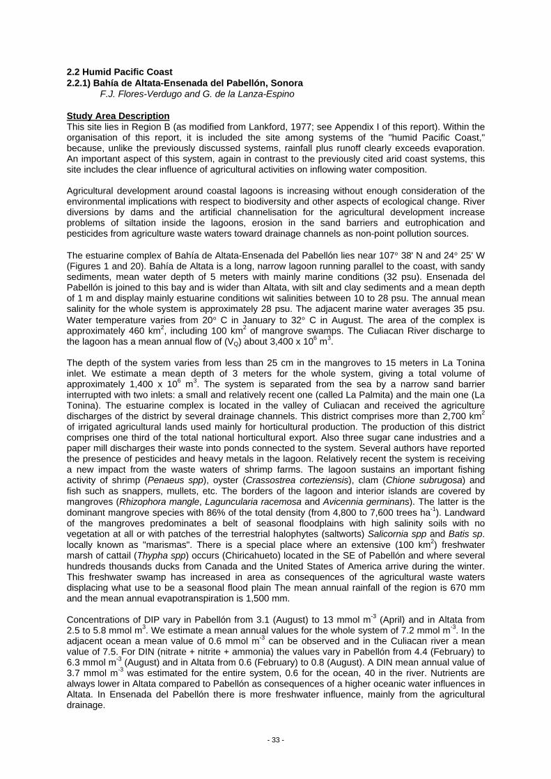
The estuarine complex of Bahía de Altata-Ensenada del Pabellón lies near 107° 38' N and 24° 25' W(Figures 1 and 20). Bahía de Altata is a long, narrow lagoon running parallel to the coast, with sandysediments, mean water depth of 5 meters with mainly marine conditions (32 psu). Ensenada delPabellón is joined to this bay and is wider than Altata, with silt and clay sediments and a mean depthof 1 m and display mainly estuarine conditions wit salinities between 10 to 28 psu. The annual meansalinity for the whole system is approximately 28 psu. The adjacent marine water averages 35 psu.Water temperature varies from 20° C in January to 32° C in August. The area of the complex isapproximately 460 km2, including 100 km2 of mangrove swamps. The Culiacan River discharge tothe lagoon has a mean annual flow of (VQ) about 3,400 x 106 m3.
The depth of the system varies from less than 25 cm in the mangroves to 15 meters in La Toninainlet. We estimate a mean depth of 3 meters for the whole system, giving a total volume ofapproximately 1,400 x 106 m3. The system is separated from the sea by a narrow sand barrierinterrupted with two inlets: a small and relatively recent one (called La Palmita) and the main one (LaTonina). The estuarine complex is located in the valley of Culiacan and received the agriculturedischarges of the district by several drainage channels. This district comprises more than 2,700 km2
of irrigated agricultural lands used mainly for horticultural production. The production of this districtcomprises one third of the total national horticultural export. Also three sugar cane industries and apaper mill discharges their waste into ponds connected to the system. Several authors have reportedthe presence of pesticides and heavy metals in the lagoon. Relatively recent the system is receivinga new impact from the waste waters of shrimp farms. The lagoon sustains an important fishingactivity of shrimp (Penaeus spp), oyster (Crassostrea corteziensis), clam (Chione subrugosa) andfish such as snappers, mullets, etc. The borders of the lagoon and interior islands are covered bymangroves (Rhizophora mangle, Laguncularia racemosa and Avicennia germinans). The latter is thedominant mangrove species with 86% of the total density (from 4,800 to 7,600 trees ha-1). Landwardof the mangroves predominates a belt of seasonal floodplains with high salinity soils with novegetation at all or with patches of the terrestrial halophytes (saltworts) Salicornia spp and Batis sp.locally known as "marismas". There is a special place where an extensive (100 km2) freshwatermarsh of cattail (Thypha spp) occurs (Chiricahueto) located in the SE of Pabellón and where severalhundreds thousands ducks from Canada and the United States of America arrive during the winter.This freshwater swamp has increased in area as consequences of the agricultural waste watersdisplacing what use to be a seasonal flood plain The mean annual rainfall of the region is 670 mmand the mean annual evapotranspiration is 1,500 mm.
Concentrations of DIP vary in Pabellón from 3.1 (August) to 13 mmol m-3 (April) and in Altata from2.5 to 5.8 mmol m3. We estimate a mean annual values for the whole system of 7.2 mmol m-3. In theadjacent ocean a mean value of 0.6 mmol m-3 can be observed and in the Culiacan river a meanvalue of 7.5. For DIN (nitrate + nitrite + ammonia) the values vary in Pabellón from 4.4 (February) to6.3 mmol m-3 (August) and in Altata from 0.6 (February) to 0.8 (August). A DIN mean annual value of3.7 mmol m-3 was estimated for the entire system, 0.6 for the ocean, 40 in the river. Nutrients arealways lower in Altata compared to Pabellón as consequences of a higher oceanic water influences inAltata. In Ensenada del Pabellón there is more freshwater influence, mainly from the agriculturaldrainage.
- 34 -
Nutrients cycling from the sediments to the water were estimated to be as high as 0.6 mmol m-2 day-1
for ammonium and of 0.05 mmol m-2 day-1 for phosphate. In lagoon sediments influenced by sugarcane waste water values as high as 16 mmol m-2 day-1 for ammonium and 2,2 mmol m-2 day-1 forphosphate were detected, demonstrating that eutrophication is a clear problem in some parts of thissystem.
Plankton net annual productivity (p) was estimated to be of 267 g C m-3 year-1, equivalent to about 70mol C m-2 year-1 The water column has a p/r ratio of 2.0 describing this part of the system asautotrophic in general.
Figure 20. Map of Bahía de Altata-Ensenada del Pabellón.
- 35 -
Water and Salt Budgets
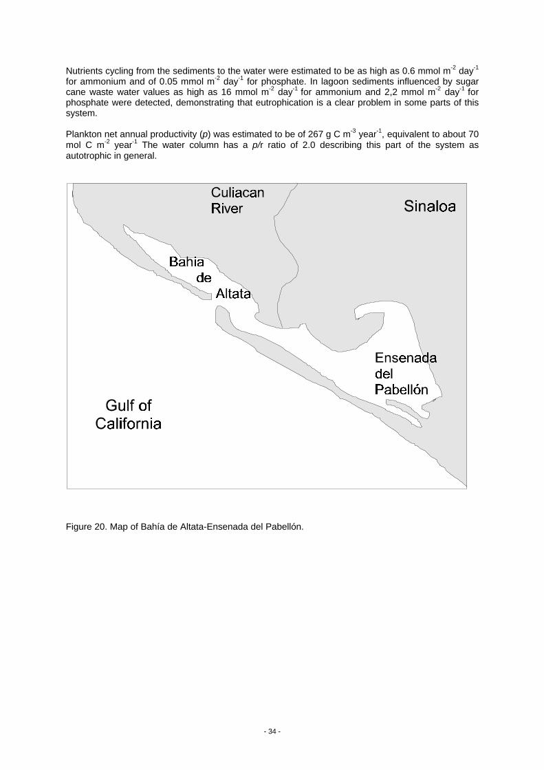
Figure 21 summarises the water and salt budgets for this system. Runoff (VQ) + precipitation (VP)substantially exceed evaporation (VE), and groundwater input (VG) is assumed to be zero. In order tobalance the water budget, residual flow removes water and salt from the system (VR = -3,000 x 106
m3 year-1; VRSR = -94,500 x 106 psu m3 year-1). In order to maintain a steady state salinity (that isVsystemdSsystem/dt = 0), salt must mix into the system (VX[Socean-Ssystem] = +94,500 x 106 psu m3 year-1).Socean and Ssystem are known, so we can solve for mixing (VX = 13,500 x 106 m3 year-1). The volume ofthe system is 1,400 x 106 m3, so water exchange time can be calculated as τ = Vsystem/(|VR| + VX) =0.08 year. That is, the water exchange time is about 1 month.
Figure 21. Water and salt budgets for Bahía Altata-Ensenada del Pabellón, annual average. Systemvolume in 106 m3. Water fluxes in 106 m3 year-1. Salt fluxes in 106 psu m3 year-1.
VQ = 3,400
VE = - 700VP = +300
VSystem = 1,400
SSystem = 28 psu
τ = 0.08 years
VR = -3,000VRSR = -94,500
SOcean = 35.0 psuSR = 31.5 psu
VX (SOcean -SSystem) = +94,500
VX = + 13,500
VG = VO = 0(assumed)
- 36 -
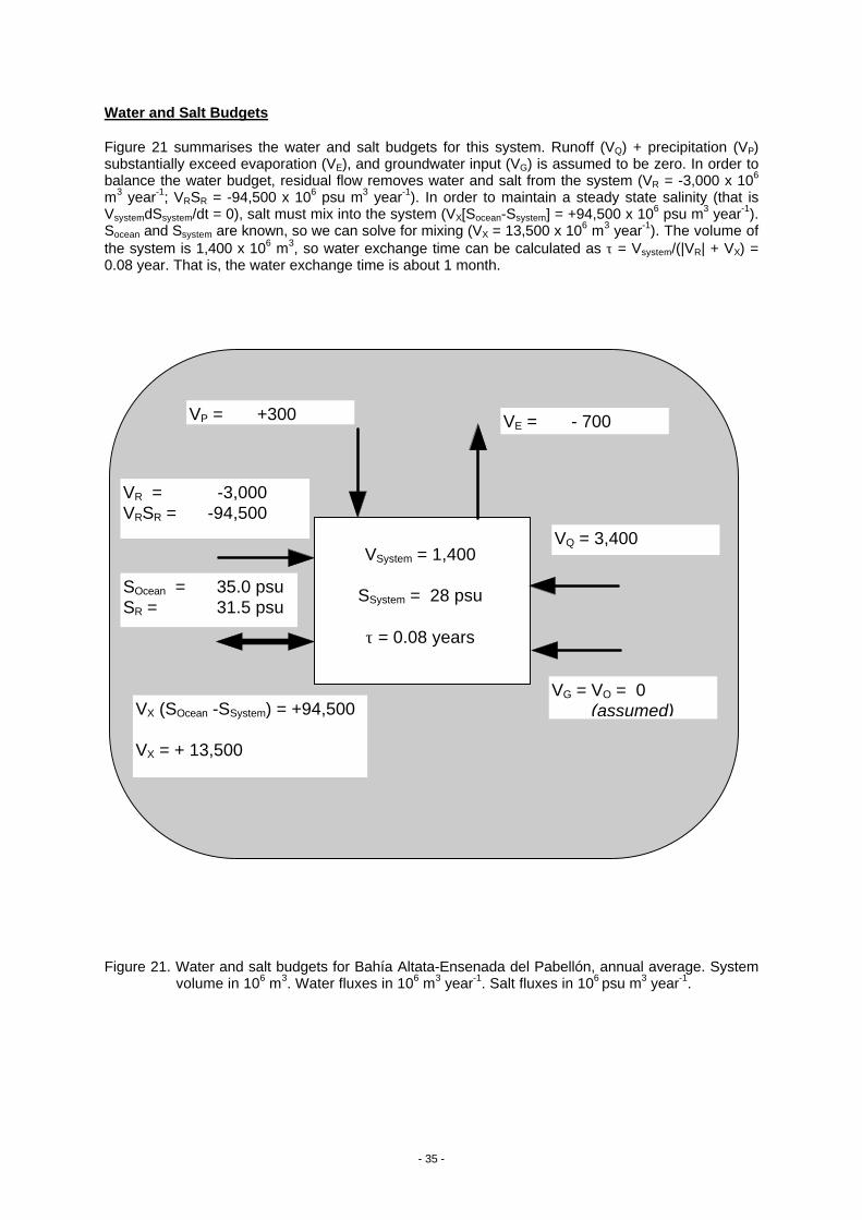
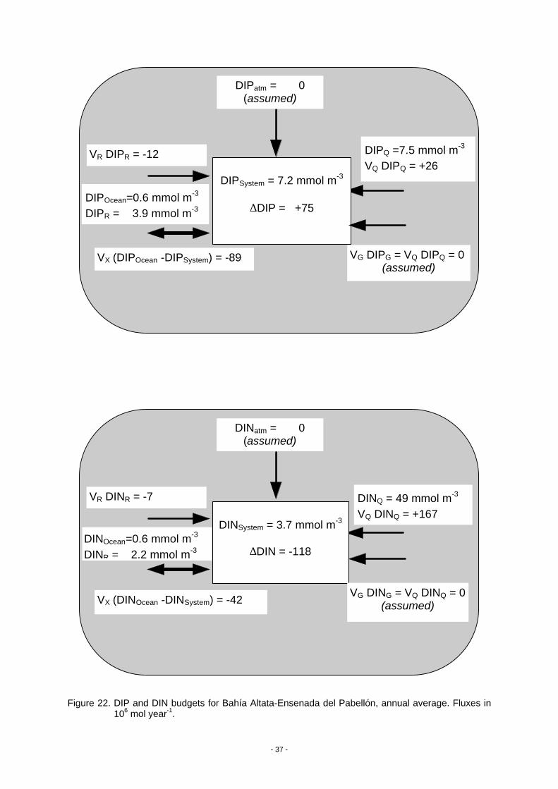
Budgets of Nonconservative MaterialsFigure 22 summarises the DIP and DIN budgets for the system.
P Balance
Concentration and flux of DIP in river water flowing into this system are high, apparently reflectingthe product of agricultural drainage into the system. System concentrations are also very high, andoutward transport of DIP occurs via both residual flow and mixing. These outward fluxes greatlyexceed the estimated river inflow of DIP, so there apparently is an internal source of DIP (∆DIP =+75 x 106 mol year-1 = +0.19 mol m-2 year-1). We have observed that there is very high release ofDIP, especially from the sediments associated with sugar cane wastes, so this and other organicdischarges into the system are assumed to support the high nonconservative flux of DIP.
N Balance
Concentration and flux of DIN in river water are also high. While there is export of DIN both in theresidual flow and in the mixing, this outward flux is substantially lower than the river DIN import.There must therefore be a substantial sink of DIN in this system (∆DIN = -118 x 106 mol year-1 = -0.46 mol m-2 year-1). There is thus a clear discrepancy between the nonconservative fluxes of DIPand DIN.
Stoichiometric Calculations of Aspects of Net System Metabolism
Net nitrogen fixation minus denitrification in this system (nfix-denit) is calculated as the differencebetween observed and expected ∆DIN. Expected ∆DIN is ∆DIP multiplied by the N:P ratio of thereacting particulate organic matter. We do not know that N:P ratio. If this material were plankton, theexpected ratio would be near the Redfield Ratio of 16:1. Waste from sugar cane or other terrestrialplant material might have a higher ratio, while animal wastes might be somewhat lower. Lacking adefinitive value, we assume that the appropriate N:P ratio of decomposing organic matter is near theRedfield Ratio, and therefore that the expected value for ∆DIN is 16 x (75 x 106) mol year-1. Thus:
(nfix-denit) = -118 x 106 - 16 x (75 x 106) mol year-1 = -1,082 x 106 mol year--1
(-2.4 mol N m-2 year-1 over the area of the system).
Thus, the system appears to be denitrifying at a substantial rate.
We can also estimate net ecosystem metabolism (NEM), that is the difference between primaryproduction and respiration (p-r), as the negative of the nonconservative DIP flux multiplied by theC:P ratio of the reacting material. Again, we do not know the C:P ratio of the reacting material, but itseems likely to equal or exceed the C:P ratio of plankton. Thus:
(p-r) = -106 x (75 x 106 mol year-1) = -7,950 x 106 mol C year-1
(-17 mol m-2 year-1 over the system area).
This is a substantial rate of net respiration, especially when compared with the estimated of primaryproduction (17 mol C m-2 year-1). Moreover, if the reacting material is terrigenous plant organicmatter, the likely rate of (p-r) may well exceed what is estimated here. Nevertheless, we believe thatthese numbers make sense in view of the discharge of sugar cane and other agricultural wasteproducts into this system.
- 37 -
Figure 22. DIP and DIN budgets for Bahía Altata-Ensenada del Pabellón, annual average. Fluxes in106 mol year-1.
DIPQ =7.5 mmol m-3
VQ DIPQ = +26
DIPatm = 0(assumed)
DIPSystem = 7.2 mmol m-3
∆DIP = +75
VR DIPR = -12
DIPOcean=0.6 mmol m-3
DIPR = 3.9 mmol m-3
VX (DIPOcean -DIPSystem) = -89 VG DIPG = VQ DIPQ = 0(assumed)
DINQ = 49 mmol m-3
VQ DINQ = +167
DINatm = 0(assumed)
DINSystem = 3.7 mmol m-3
∆DIN = -118
VR DINR = -7
VX (DINOcean -DINSystem) = -42VG DING = VQ DINQ = 0
(assumed)
DINOcean=0.6 mmol m-3
DINR = 2.2 mmol m-3
- 38 -
2.2.2) Teacapan-Agua Brava- Marismas Nacionales, Sinaloa and NayaritG. de la Lanza-Espino, F. J. Flores-Verdugo and F. Wulff
Study Area DescriptionFigures 1 and 23 illustrate the location and principal features of the mangrove-estuarine complex ofTeacapan-Agua Brava-Marismas Nacionales (22° 08’ N, 105° 32’ W). A brief historical and naturalhistory perspective is presented in the next paragraphs.
The region of Teacapan-Agua Brava-Marismas Nacionales has an ancient story for humansettlements. There are evidences of considerable human populations over more than 1,500 years, inthe forms of small hills of shells (Tivela sp.). Near the town of Mexcaltitan a tribal group migrated tothe upper lands and founded the city of Tenochtitlan (now Mexico city), the capital of the Aztecempire. When the Spaniards arrived in the region in the 16th century, they estimated a population ofmore than 300,000 inhabitants; this can be considered extremely high for rural standards of thosedays. This high population density was sustained by the fertility of the land in the alluvial plain butalso to the richness of seafood as oyster, shrimp and fishes. The region has been a used by severalgenerations for multiple uses. Mangroves where mainly used for fuel and rustic construction, duringthe colonial age, an important industry of tannins for cow hide treatment was developed until the 19thcentury. The region was an important hunting ground up to the 1950’s for jaguar and crocodile. In thewinter, more than the 20% of the total migratory birds of the Pacific arrive enroute from Alaska,Canada and the United States. It is also possible to find areas with subhumid tropical forest and lowhuman impact between the mangroves on some islands. The region indirectly supports one of themost important shark fishery in Mexico in the adjacent marine waters. Shrimp fishing is an importanteconomical activity and recently shrimp farming is developing. In the beginning of the 1970’s anartificial inlet was opened (Cuautla Channel) with the idea to allow the shrimp post-larvae get insidethe Agua Brava lagoon more directly, but the channel widened uncontrollably from 40 m wide 3 mdepth, as was planned, to more than 1,200 m wide and 18 m depth. The drastic change in thehydrological pattern killed more than 50 km2 of mangroves. The aquaculture development withoutplanning with an environmental sound management, the river dam construction programs togetherwith the agricultural activities and the opening of artificial inlets, will put at risk the basic structuralfunctions of the ecosystem and this actual and potential resources as important cultural values.
The area comprises approximately 2,000 km2 of tidal channels, seasonal flood plains, more than 150semi-parallel coastal lagoons formed by stranded beach ridges, big estuarine water bodies andmangrove swamps. The mangroves, small tidal channels and the semi-parallel coastal lagoonsoccupies approximately 1,100 km2. The waterways occupy 500 km2 (total area of the mangrove-estuarine complex 1,600 km2). Water depths of the waterways vary from below 1 m to 18 m near theinlets, with a mean depth of 2 m. The mangrove water depth varies according to the species, being0.40 m above mean sea level for the dominant species, the white mangrove (Lagunculariaracemosa) and 0.7 m for the black mangrove (Avicenia germinans) we assume that during theflooding periods (flows) a mean value of 0.5 m is reasonable. Obviously 0.0 m depth is assumedduring low ebb tides. A mean value (flows and ebbs) of 0.25 m is considered here to be appropriate.The total volume (V1) of the mangrove-estuarine complex comprises 1,266 x 106 m3.
There are 5 stream flows that discharge to the system: The Cañas, Rosamorada, Bejuco, Acaponetaand San Pedro rivers. But only the last two have flow all year around, with an annual flow of 3,000 x106 m3 year-1 for the Acaponeta and 2,456 x 106 m3 year-1 for the San Pedro river. The other riversare seasonal with flows below 180 x 106 m3 year-1. Precipitation is estimated to be about 1,459 mmyear-1 and evapotranspiration of 1,991 mm year-1 (mean annual values of more than 10 years). Dataon groundwater flow and non-point agriculture waste-waters that discharge to the system are notavailable.
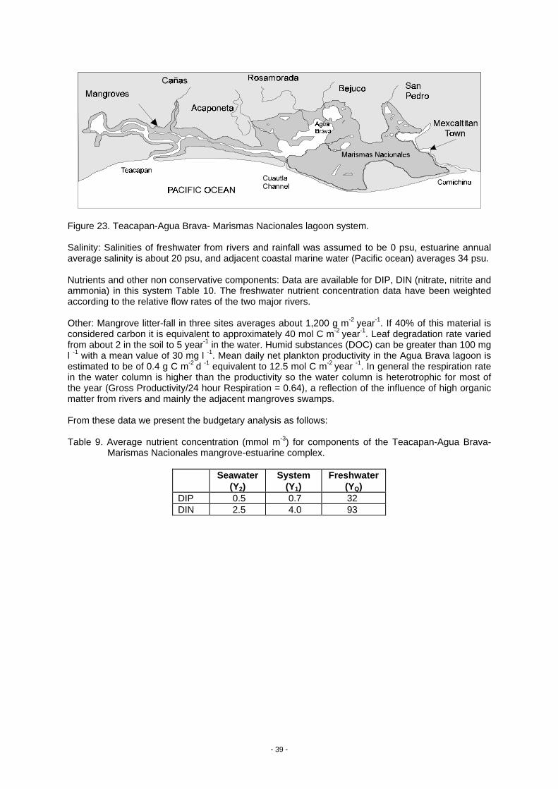
- 39 -
Figure 23. Teacapan-Agua Brava- Marismas Nacionales lagoon system.
Salinity: Salinities of freshwater from rivers and rainfall was assumed to be 0 psu, estuarine annualaverage salinity is about 20 psu, and adjacent coastal marine water (Pacific ocean) averages 34 psu.
Nutrients and other non conservative components: Data are available for DIP, DIN (nitrate, nitrite andammonia) in this system Table 10. The freshwater nutrient concentration data have been weightedaccording to the relative flow rates of the two major rivers.
Other: Mangrove litter-fall in three sites averages about 1,200 g m-2 year-1. If 40% of this material isconsidered carbon it is equivalent to approximately 40 mol C m-2 year-1. Leaf degradation rate variedfrom about 2 in the soil to 5 year-1 in the water. Humid substances (DOC) can be greater than 100 mgl -1 with a mean value of 30 mg l -1. Mean daily net plankton productivity in the Agua Brava lagoon isestimated to be of 0.4 g C m-2 d -1 equivalent to 12.5 mol C m-2 year -1. In general the respiration ratein the water column is higher than the productivity so the water column is heterotrophic for most ofthe year (Gross Productivity/24 hour Respiration = 0.64), a reflection of the influence of high organicmatter from rivers and mainly the adjacent mangroves swamps.
From these data we present the budgetary analysis as follows:
Table 9. Average nutrient concentration (mmol m-3) for components of the Teacapan-Agua Brava-Marismas Nacionales mangrove-estuarine complex.
Seawater(Y2)
System(Y1)
Freshwater(YQ)
DIP 0.5 0.7 32DIN 2.5 4.0 93

- 40 -
Water and Salt Budgets
Figure 24 illustrates the average annual water and salt budgets for Teacapan-Agua Brava-MarismasNacionales. Freshwater flow (VQ ) is estimated by adding the flows of the Acaponeta and San Pedrorivers (5,456 x 106 m3 year-1). Direct precipitation (Vp) and Evaporation (VE) are estimated as 2,412 x106 m3 year-1 and 3,223 x 106 m3 year-1, respectively, considering the area of the complex (1,619 x106 m2 ). The other components (VG and Vo) are assumed to be small. The system shows substantialnet residual outflow of water, as expected from the freshwater inputs to the system. It can be seenfrom these calculations that the water exchange time in this system is about a month.
Figure 24. Water and salt budgets for Teacapan-Agua Brava-Marismas Nacionales, annual average.System volume is in units of 106 m3. Water fluxes in 106 m3 year-1. Salt fluxes in 106 psum3 year-1.
VQ = 5,500
VE = - 3,200VP = + 2,400
VSystem = 1,266
SSystem = 20 psu
τ = 0.10 years
VR = -4,400VRSR = -118,800
SOcean = 34 psuSR = 27 psu
VX (SOcean - SSystem) = +118,800
VX = + 8,486
VG = VO = 0(assumed)
- 41 -
Budgets of Nonconservative MaterialsFigure 25 illustrates the DIP and DIN budgets for these systems. The data are also listed in Tables10-13.
P Balance
Substantial DIP comes in from terrigenous runoff into this system, but very little P exchanges withthe ocean with either residual flow or exchange flow. Clearly the system takes up most of the DIPdelivered to it. The system is a sink for virtually all of the land derived DIP (Figure 25). Thus, ∆DIP =-170 x 106 mol year-1 = -0.11 mol m-2 year-1 over the mangrove-estuary area.
N Balance
Similarly to DIP, DIN comes in from land and is mostly trapped in the system (Figure 25). Thus, ∆DIN= -452 x 106 mol year-1 = -0.28 mol m-2 year-1 over the mangrove-estuary area.
Stoichiometric Calculation of Aspects of Net System Metabolism
We can calculate net nitrogen fixation minus denitrification (nfix-denit) as the difference betweenobserved and expected ∆DIN. Expected ∆DIN is ∆DIP multiplied by the N:P ratio of the reactingparticulate organic matter. In a mangrove-dominated system, it is not entirely obvious what thedominating reactive organic matter is, so we use two N:P values. First, we employ the Redfield N:Pratio of plankton (16:1). Then we use a reactant which has an N:P ratio of 30:1, more typical ofvarious land plants. Thus, with plankton:
(nfix-denit) = -452 x 106 – 16 x (-170 x 106) = +2,268 x 106 mol N year-1
(+1.4 mol N m-2 year-1 over the estuary-mangrove area).
With land plants:
(nfix-denit) = -452 x 106 – 30 x (-170 x 106) = +46,448 x 106 mol N year-1
(+2.9 mol N m-2 year-1 over the estuary-mangrove area).
Note that, with either material, the system appears likely to be fixing nitrogen in excess ofdenitrification.
Similarly, we can estimate net ecosystem metabolism (NEM = p-r) as the negative of thenonconservative DIP flux multiplied by the C:P ratio of the reacting organic matter. If the net reactingmaterial is plankton, the particulate C:P ratio is about 106:1. If it is mangrove litter, then the ratio maybe as high as 1000:1. With plankton:
(p-r) = -106 x (-170 x 106) = +18,020 x 106 mol C year-1
(+11 mol C m-2 year-1).
With mangroves dominating the net production:
(p-r) = -1,000 x (-170 x 106) = +170,000 x 106 mol C year-1
(+106 mol C m-2 year-1).
This latter figure is about double the rate of mangrove litter production, and that production shouldapproach an upper limit of net primary production. We therefore suggest that the lower figure moreaccurately reflects the likely rate of net ecosystem production. In either case, if the DIP uptakeprimarily represents net organic metabolism, rather than inorganic sorption or precipitation of P, thissystem is strongly net autotrophic.
We assume that the lower value more accurately reflects (p-r). Primary production was estimatedabove to be about 30 mol C m-2 year-1, implying that respiration is approximately 30. These numberssuggest that the p/r ratio of the system is about 1.3.
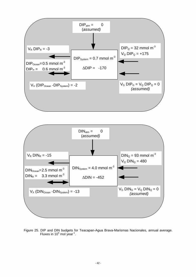
- 42 -
Figure 25. DIP and DIN budgets for Teacapan-Agua Brava-Marismas Nacionales, annual average.Fluxes in 106 mol year-1.
DIPQ = 32 mmol m-3
VQ DIPQ = +175
DIPatm = 0(assumed)
DIPSystem = 0.7 mmol m-3
∆DIP = -170
VR DIPR = -3
DIPOcean=0.5 mmol m-3
DIPR = 0.6 mmol m-3
VX (DIPOcean -DIPSystem) = -2 VG DIPG = VQ DIPQ = 0(assumed)
DINQ = 93 mmol m-3
VQ DINQ = 480
DINatm = 0(assumed)
DINSystem = 4.0 mmol m-3
∆DIN = -452
VR DINR = -15
VX (DINOcean -DINSystem) = -13 VG DING = VQ DINQ = 0(assumed)
DINOcean=2.5 mmol m-3
DINR = 3.3 mmol m-3
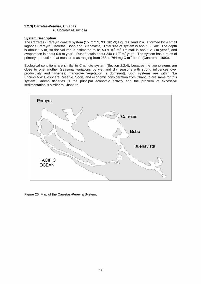
- 43 -
2.2.3) Carretas-Pereyra, ChiapasF. Contreras-Espinosa
System DescriptionThe Carretas - Pereyra coastal system (15° 27' N, 93° 10' W; Figures 1and 26), is formed by 4 smalllagoons (Pereyra, Carretas, Bobo and Buenavista). Total size of system is about 35 km2. The depthis about 1.5 m, so the volume is estimated to be 53 x 106 m3. Rainfall is about 2.3 m year-1, andevaporation is about 0.8 m year-1. Runoff totals about 240 x 106 m3 year-1. The system has a rates ofprimary production that measured as ranging from 288 to 764 mg C m-3 hour-1 (Contreras, 1993).
Ecological conditions are similar to Chantuto system (Section 2.2.4), because the two systems areclose to one another (seasonal variations by wet and dry seasons with strong influences overproductivity and fisheries; mangrove vegetation is dominant). Both systems are within “LaEncrucijada” Biosphere Reserve. Social and economic consideration from Chantuto are same for thissystem. Shrimp fisheries is the principal economic activity and the problem of excessivesedimentation is similar to Chantuto.
Figure 26. Map of the Carretas-Pereyra System.

- 44 -
Water and Salt Budgets
Figure 27 summarises the water and salt budgets for this system. Runoff into this system is about230 x 106 m3 year-1; rainfall is about 80 x 106 m3 year-1; and evaporation is about 20 x 106 m3 year-1.Therefore residual flow out of this system totals about 300 x 106 m3 year-1. We assume thatfreshwater inflow has a salinity of 0 psu. Oceanic salinity adjacent to the lagoon is estimated to havea salinity of about 21.6 psu, and the average lagoon salinity is about 10.8 psu. With these figures awater exchange time of about 0.07 years (~ 26 days) is calculated.
Figure 27. Water and salt budgets for Carretas-Pereyra, annual average. System volume is in unitsof 106 m3 . Water fluxes in 106 m3 year-1. Salt fluxes in 106 psu m3 year-1.
VQ = +234
VE = - 24VP = + 79
VSystem = 53
SSystem = 10.8 psu
τ = 0.07 years
VR = -297VRSR = -4,682
SOcean = 21.6 psuSR = 16.2 psu
VX (SOcean - SSystem) = +4,682
VX = + +434
VG = VO = 0(assumed)
- 45 -
Budgets of Nonconservative MaterialsFigure 28 summarises the DIP and DIN budgets for this system.
P Balance
DIP concentration in the Carretas-Pereyra lagoonal complex is relatively high and riverine input islow. As a result, the calculations indicate that ∆DIP is positive (+3 x 10⁶ mol year-1). This isequivalent to a flux of 0.09 mol m-2 year-1.
N Balance
Similarly, there is a positive nonconservative flux of DIN within this system (∆DIN = 3 x 10⁶ mol year-
1; 0.09 mmol m-2 year-1).
Stoichiometric Calculations of Aspects of Net System Metabolism
Net nitrogen fixation minus denitrification (nfix-denit) is calculated as the difference betweenobserved and expected ∆DIN. Expected ∆DIN is ∆DIP multiplied by the N:P ratio of the reactingparticulate organic matter. In a mangrove-dominated system, it is not entirely obvious what thedominating reactive organic matter is, so we use two N:P values. First, we employ the Redfield N:Pratio of plankton (16:1). Then we use a reactant which has an N:P ratio of 30:1, more typical ofvarious land plants. Thus, with plankton:
(nfix-denit) = +3 x 10⁶ – 16 x (+3 x 10⁶) = -45 x 106 mol N year-1
(-1.2 mol N m-2 year-1 over the estuary area).
With land plants:
(nfix-denit) = +3 x 10⁶ – 30 x (3 x 106 ) = -87 x 106 mol N year-1(-2.5 mol N m-2 year-1 over the estuary area).
Note that, with either material, the system appears likely to be a net denitrification system.
Similarly, we can estimate net ecosystem metabolism (NEM = p-r) as the negative of thenonconservative DIP flux multiplied by the C:P ratio of the reacting organic matter. If the net reactingmaterial is plankton, the particulate C:P ratio is about 106:1. If it is mangrove litter, then the ratio maybe as high as 1000:1. With plankton:
(p-r) = -106 x (+3 x 10⁶ ) = -318 x 106 mol C year-1
(-9 mol C m-2 year-1)
With mangroves dominating the net metabolism:
(p-r) = -1,000 x (+3 x 10⁶) = +3,000 x 106 mol C year-1
(+86 mol C m-2 year-1).
This latter figure is about double the likely rate of mangrove litter production (based on data fromAgua Brava), and that production should approach an upper limit of net primary production. Wetherefore suggest that the lower figure more accurately reflects the likely rate of net ecosystemproduction. In either case, if the DIP uptake primarily represents net organic metabolism, rather thaninorganic sorption or precipitation of P, this system is net heterotrophic.
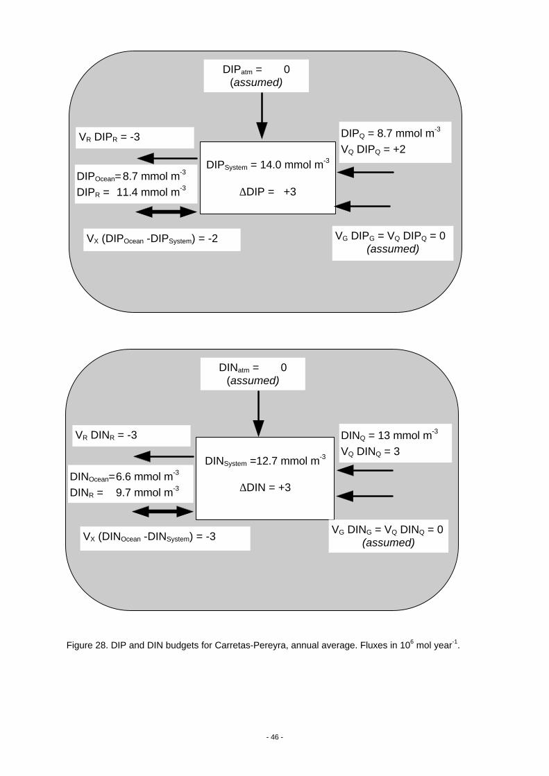
- 46 -
Figure 28. DIP and DIN budgets for Carretas-Pereyra, annual average. Fluxes in 106 mol year-1.
DIPQ = 8.7 mmol m-3
VQ DIPQ = +2
DIPatm = 0(assumed)
DIPSystem = 14.0 mmol m-3
∆DIP = +3
VR DIPR = -3
DIPOcean=8.7 mmol m-3
DIPR = 11.4 mmol m-3
VX (DIPOcean -DIPSystem) = -2 VG DIPG = VQ DIPQ = 0(assumed)
DINQ = 13 mmol m-3
VQ DINQ = 3
DINatm = 0(assumed)
DINSystem =12.7 mmol m-3
∆DIN = +3
VR DINR = -3
VX (DINOcean -DINSystem) = -3 VG DING = VQ DINQ = 0(assumed)
DINOcean=6.6 mmol m-3
DINR = 9.7 mmol m-3
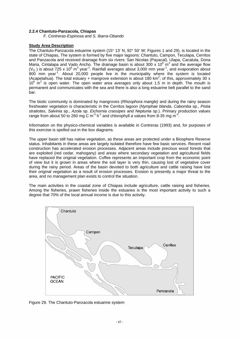
- 47 -
2.2.4 Chantuto-Panzacola, ChiapasF. Contreras-Espinosa and S. Ibarra-Obando
Study Area DescriptionThe Chantuto-Panzacola estuarine system (15° 13’ N, 92° 50’ W; Figures 1 and 29), is located in thestate of Chiapas, The system is formed by five major lagoons: Chantuto, Campon, Teculapa, Cerritosand Panzacola and received drainage from six rivers: San Nicolas (Payacal), Ulapa, Cacaluta, DonaMaria, Cintalapa and Vado Ancho. The drainage basin is about 300 x 106 m3 and the average flow(VQ ) is about 725 x 106 m3 year-1. Rainfall averages about 3,000 mm year-1, and evaporation about800 mm year-1. About 20,000 people live in the municipality where the system is located(Acapetahua). The total estuary + mangrove extension is about 180 km2; of this, approximately 30 x106 m2 is open water. The open water area averages only about 1.5 m in depth. The mouth ispermanent and communicates with the sea and there is also a long estuarine belt parallel to the sandbar.
The biotic community is dominated by mangroves (Rhizophora mangle) and during the rainy seasonfreshwater vegetation is characteristic in the Cerritos lagoon (Nymphae blanda, Cabomba sp., Pistiastratiotes, Salvinia sp., Azola sp. Eichornia crassipes and Neptunia sp.). Primary production valuesrange from about 50 to 260 mg C m-3 h-1 and chlorophyll a values from 8-35 mg m-3.
Information on the physico-chemical variables is available in Contreras (1993) and, for purposes ofthis exercise is spelled out in the box diagrams.
The upper basin still has native vegetation, as these areas are protected under a Biosphere Reservestatus. Inhabitants in these areas are largely isolated therefore have few basic services. Recent roadconstruction has accelerated erosion processes. Adjacent areas include precious wood forests thatare exploited (red cedar, mahogany) and areas where secondary vegetation and agricultural fieldshave replaced the original vegetation. Coffee represents an important crop from the economic pointof view but it is grown in areas where the soil layer is very thin, causing lost of vegetative coverduring the rainy period. Areas of the basin devoted to both agriculture and cattle raising have losttheir original vegetation as a result of erosion processes. Erosion is presently a major threat to thearea, and no management plan exists to control the situation.
The main activities in the coastal zone of Chiapas include agriculture, cattle raising and fisheries.Among the fisheries, prawn fisheries inside the estuaries is the most important activity to such adegree that 70% of the local annual income is due to this activity.
Figure 29. The Chantuto-Panzacola estuarine system
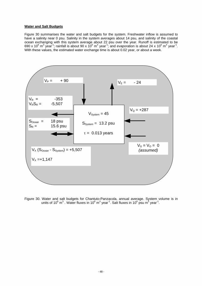
- 48 -
Water and Salt Budgets
Figure 30 summarises the water and salt budgets for the system. Freshwater inflow is assumed tohave a salinity near 0 psu. Salinity in the system averages about 14 psu, and salinity of the coastalocean exchanging with this system average about 22 psu over the year. Runoff is estimated to be690 x 106 m3 year-1; rainfall is about 90 x 106 m3 year-1; and evaporation is about 24 x 106 m3 year-1.With these values, the estimated water exchange time is about 0.02 year, or about a week.
Figure 30. Water and salt budgets for Chantuto-Panzacola, annual average. System volume is inunits of 106 m3 . Water fluxes in 106 m3 year-1. Salt fluxes in 106 psu m3 year-1.
VQ = +287
VE = - 24VP = + 90
VSystem = 45
SSystem = 13.2 psu
τ = 0.013 years
VR = -353VRSR = -5,507
SOcean = 18 psuSR = 15.6 psu
VX (SOcean - SSystem) = +5,507
VX =+1,147
VG = VO = 0(assumed)
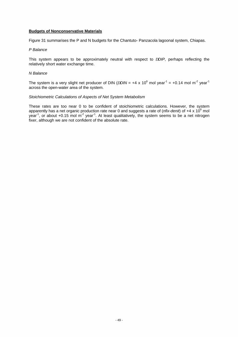
- 49 -
Budgets of Nonconservative Materials
Figure 31 summarises the P and N budgets for the Chantuto- Panzacola lagoonal system, Chiapas.
P Balance
This system appears to be approximately neutral with respect to ∆DIP, perhaps reflecting therelatively short water exchange time.
N Balance
The system is a very slight net producer of DIN (∆DIN = +4 x 10⁶ mol year-1 = +0.14 mol m-2 year-1
across the open-water area of the system.
Stoichiometric Calculations of Aspects of Net System Metabolism
These rates are too near 0 to be confident of stoichiometric calculations. However, the systemapparently has a net organic production rate near 0 and suggests a rate of (nfix-denit) of +4 x 10⁶ molyear-1, or about +0.15 mol m-2 year-1. At least qualitatively, the system seems to be a net nitrogenfixer, although we are not confident of the absolute rate.
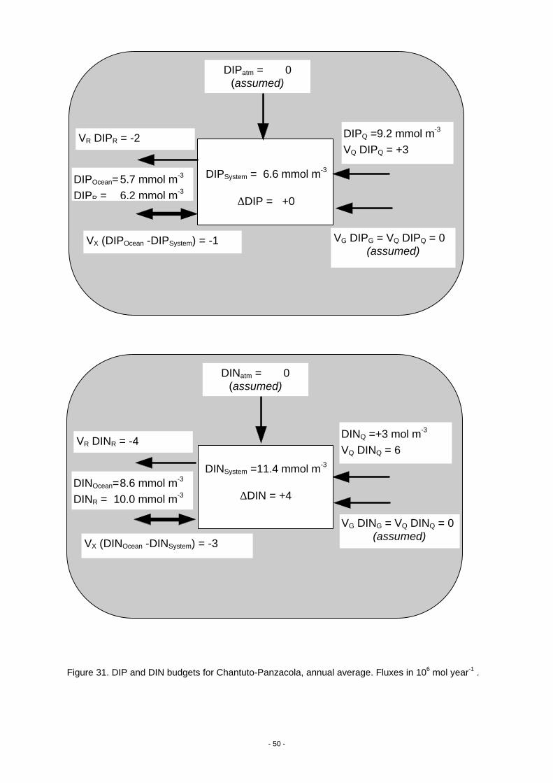
- 50 -
Figure 31. DIP and DIN budgets for Chantuto-Panzacola, annual average. Fluxes in 106 mol year-1 .
DIPQ =9.2 mmol m-3
VQ DIPQ = +3
DIPatm = 0(assumed)
DIPSystem = 6.6 mmol m-3
∆DIP = +0
VR DIPR = -2
DIPOcean=5.7 mmol m-3
DIPR = 6.2 mmol m-3
VX (DIPOcean -DIPSystem) = -1 VG DIPG = VQ DIPQ = 0(assumed)
DINQ =+3 mol m-3
VQ DINQ = 6
DINatm = 0(assumed)
DINSystem =11.4 mmol m-3
∆DIN = +4
VR DINR = -4
VX (DINOcean -DINSystem) = -3
VG DING = VQ DINQ = 0(assumed)
DINOcean=8.6 mmol m-3
DINR = 10.0 mmol m-3
- 51 -
2.3 Gulf of Mexico
2.3.1) Laguna Madre, TamaulipasS. Ibarra-Obando and F. Contreras-Espinosa
Study Area DescriptionLaguna Madre (Figures 1 and 32, 23-25o N, 97o W) is located on the Gulf of Mexico shoreline. Itsnorthern limit is the Rio Bravo delta, and its southern limit the mouth of the Soto La Marina river. Itoccupies a shallow basin that has an average depth of 0.7 m, and an area of about 2,000 km2; it isthe largest Mexican lagoon. It is separated from the sea by a sand bar. The San Fernando rivermouth divides the lagoon into two sub-basins, known as North and South. The lagoon presents 13mouths that communicate with the sea only on a temporal basis, as sediment accumulation aftercyclones and hurricanes promotes their closure (Contreras, 1993).
Climate is arid with evaporation being far more important than freshwater input from rivers. As aconsequence, the lagoon is drying out, with increasing salinity in the remaining water body, and saltdeposition in its margins. Average evaporation is 1,900 mm year-1, and average precipitation 600mm year-1. River freshwater input which might flow into the system is diverted for agricultural andurban purposes, so none gets into the lagoon (Estado de Tamaulipas, 1996).
Dune vegetation exists at the lagoon margins, being represented by the following species: Uniolapaniculata, Ipomoea pescaprae and Croton punctulatus. Halophytes like Spartina spartinae, Suaedanigrica, Salicornia ambigua and Distichlis spicata, are also found. Upland areas present both spinyshrubs and low forest spiny species, like mesquite and ebony. Submerged vegetation consist ofalgae and seagrasses, which have been greatly reduced by the desiccation process and hypersalineconditions. Only after heavy rains and mouth openings, salinity decreases, but this effect is onlytemporary (Contreras, 1993). Halophytes are also disappearing from the lagoon margins, promotingerosional areas that also contribute to lagoon infilling (Estado de Tamaulipas, 1996).
The icthyofauna comprises 78 species, among which prawns, croakers, snooks, mullets andhoundsharks are the most representative (Contreras, 1993). Oyster and prawn aquacultural projectshave failed due to poor water quality conditions (lack of freshwater input, and lack of a free waterexchange with the ocean). For the same reasons, crab harvest has declined. The lagoon is also wellknown for being a resting, feeding and reproductive site for migratory waterfowl, mainly ducks:Aythya americana and Anas discors (Estado de Tamaulipas, 1996).
Urban wastewater, as well as pesticides, herbicides and fertilisers residues represent the mainpollution source. Boat traffic contributes to pollution by oil and fuel spill, as well as boat washing.Pollutant products are spilled in the open ocean without any regulation. All these products are carriedaway by currents and end up in the lagoon (Tamaulipas State Government, 1996).
About 80,000 people inhabit the area around the lagoon. The coastal plain represents one of themost important agricultural areas of the country, being among the most important crops: cotton,cereals, leguminous and oily crops. Cattle raising is also an economically important activity. Besidesthe artesanal fishery, large scale fisheries are represented by tuna and prawn fisheries. For theLaguna Madre area, fisheries represent the most important economic activity, although the volumecaptured is small (Estado de Tamaulipas, 1996).
Phytoplankton primary production for this system has been estimated to be about 600 g C m-2 year-1
(i.e., about 50 mol C m-2 year-1).
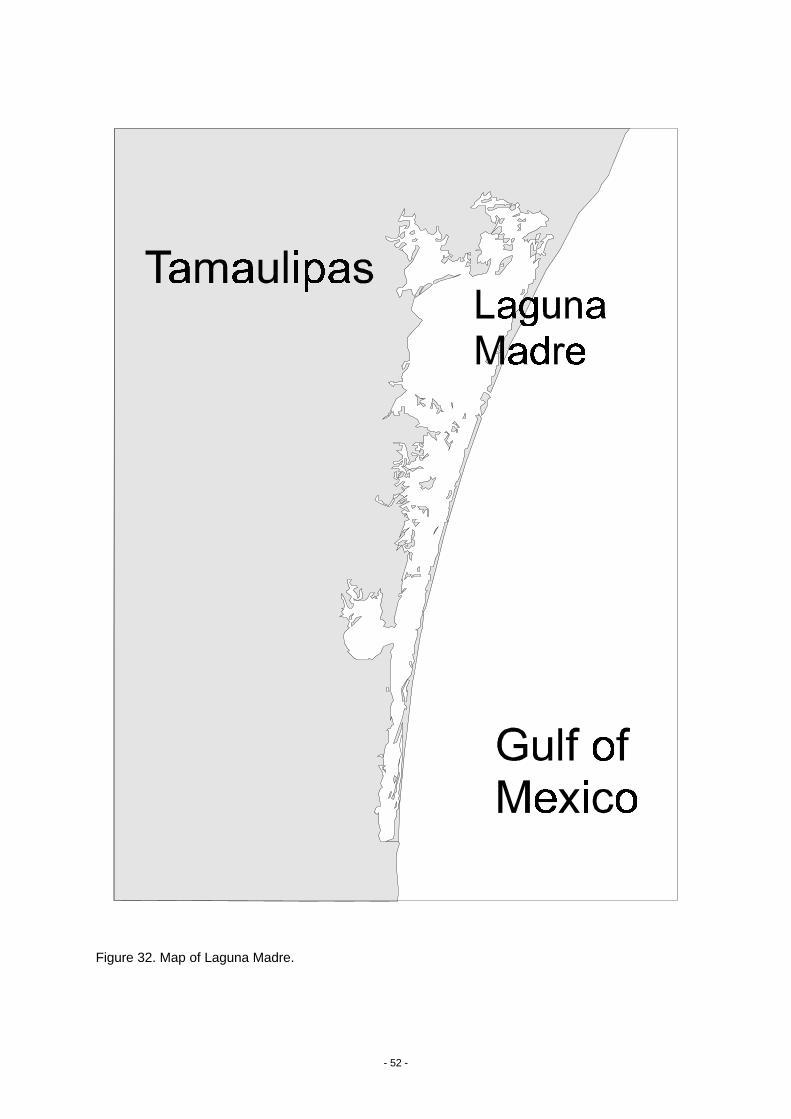
- 52 -
Figure 32. Map of Laguna Madre.
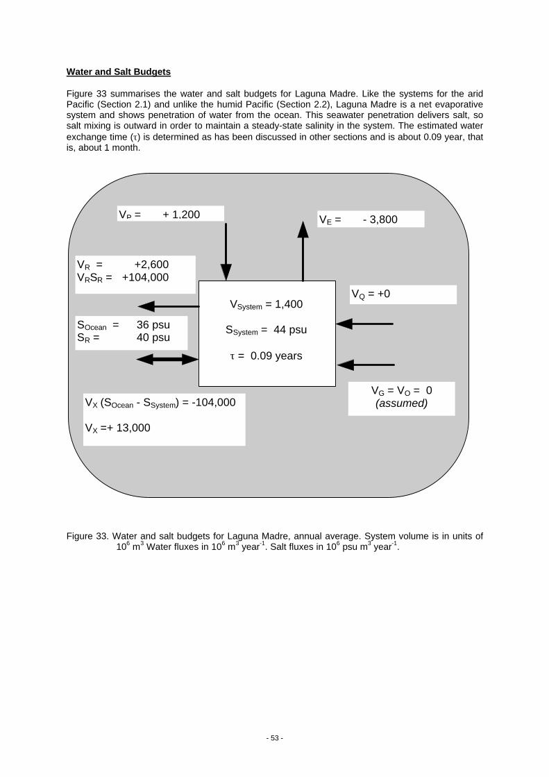
- 53 -
Water and Salt Budgets
Figure 33 summarises the water and salt budgets for Laguna Madre. Like the systems for the aridPacific (Section 2.1) and unlike the humid Pacific (Section 2.2), Laguna Madre is a net evaporativesystem and shows penetration of water from the ocean. This seawater penetration delivers salt, sosalt mixing is outward in order to maintain a steady-state salinity in the system. The estimated waterexchange time (τ) is determined as has been discussed in other sections and is about 0.09 year, thatis, about 1 month.
Figure 33. Water and salt budgets for Laguna Madre, annual average. System volume is in units of106 m3 Water fluxes in 106 m3 year-1. Salt fluxes in 106 psu m3 year-1.
VQ = +0
VE = - 3,800VP = + 1,200
VSystem = 1,400
SSystem = 44 psu
τ = 0.09 years
VR = +2,600VRSR = +104,000
SOcean = 36 psuSR = 40 psu
VX (SOcean - SSystem) = -104,000
VX =+ 13,000
VG = VO = 0(assumed)
- 54 -
Budgets of Nonconservative Materials
Figure 34 summarises the DIP and DIN budgets for this system.
P Balance
This system is a clear net source for DIP. Even though the rate of nonconservative DIP flux isrelatively small (∆DIP = +31 x 106 mol year--1 = 0.02 mol m-2 year-1), this rate results in a strongconcentration gradient between the system and the coastal ocean. The first consideration was thatthis DIP production is consistent with the production seen for the various arid systems of the aridPacific coast (section 2.1). That analogy seems to be an unlikely explanation for this phenomenon inLaguna Madre, because the oligotrophic coastal ocean waters seem unlikely to be a major source ofoceanic organic matter delivery to the lagoon. The next alternative considered was direct dischargeof human wastes. This source would deliver both organic and inorganic P; as long as the organic Pdecomposed to inorganic material, the two would be indistinguishable in the budget. If we considerthe human population living adjacent to the lagoon (80,000) and use an approximate per capita Pdischarge of 20 mol person-1 year-1, then this P source would amount to only approximately 2 x 10⁶
mol DIP year-1. It therefore seems certain that there are other sources of either direct discharge ofDIP into this system or organic P discharge and decomposition of that organic matter. Hydrocarbonpollutants and agricultural waste seem the most plausible sources. In either case, the decompositionof these materials would constitute DIP sources to sustain the apparently net heterotrophic conditionsof this system.
N Balance
This system is also a source of DIN (∆DIN = +61 x 106 mol year--1 = 0.03 mol m-2 year-1). Both NO3
and NH4 are elevated well above oceanic values (NO3System = 2.8; NO3Ocean = 0.3; NH4System = 4.6;NH4Ocean = 1.5; all units in mmol m-3). The relatively high concentrations of NH4 also tend to suggestthat the nutrient source is at least partially the result of organic decomposition.
Stoichiometric Calculations of Aspects of Net System Metabolism
Estimation of nitrogen fixation - denitrification (nfix-denit) is made from the difference betweenobserved and expected ∆DIN, where the expected value is given by ∆DIP x N:P ratio of thedecomposing organic matter. Although we do not know the source of this material, we assume that ithas an N:P ratio approximating the Redfield Ratio (16:1). Therefore:
(nfix-denit) = +61 x 106 - 16 x (+31 x 106) = -435 x 106 mol year-1
(-0.2 mol m-2 year-1 averaged over the entire lagoon).
This value is obviously uncertain, because we cannot readily predict the nature of the decomposingorganic matter. Nevertheless, the calculated rate seems reasonable.
Net ecosystem metabolism (NEM = [p-r]) can also be estimated from ∆DIP, again with theuncertainty as to the nature of the primary organic matter which is apparently decomposing. Thisquantity is estimated as the negative of ∆DIP multiplied by the C:P ratio of the reacting organicmatter. For the sake of this calculation, we assume that the reacting organic matter has anapproximately Redfield C:P ratio of 106:1. Thus:
(p-r) = -106 x (+31 x 106) = 3,286 x 106 mol year-1
(-2 mol m-2 year-1 over the lagoon area).
That is the system appears to be net heterotrophic by approximately 2 mol m-2 year-1. This value isabout 4% of the estimated annual primary production; thus the p/r ratio of this system is about 0.96.
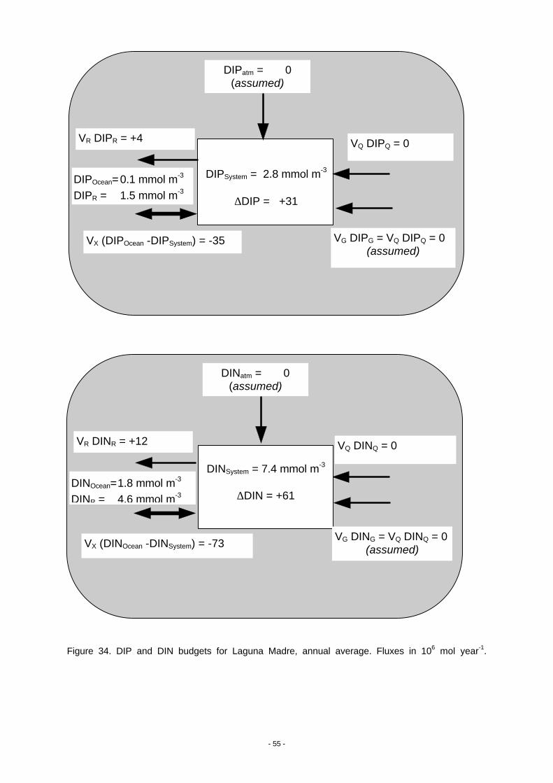
- 55 -
Figure 34. DIP and DIN budgets for Laguna Madre, annual average. Fluxes in 106 mol year-1.
VQ DIPQ = 0
DIPatm = 0(assumed)
DIPSystem = 2.8 mmol m-3
∆DIP = +31
VR DIPR = +4
DIPOcean=0.1 mmol m-3
DIPR = 1.5 mmol m-3
VX (DIPOcean -DIPSystem) = -35 VG DIPG = VQ DIPQ = 0(assumed)
VQ DINQ = 0
DINatm = 0(assumed)
DINSystem = 7.4 mmol m-3
∆DIN = +61
VR DINR = +12
VX (DINOcean -DINSystem) = -73 VG DING = VQ DINQ = 0(assumed)
DINOcean=1.8 mmol m-3
DINR = 4.6 mmol m-3
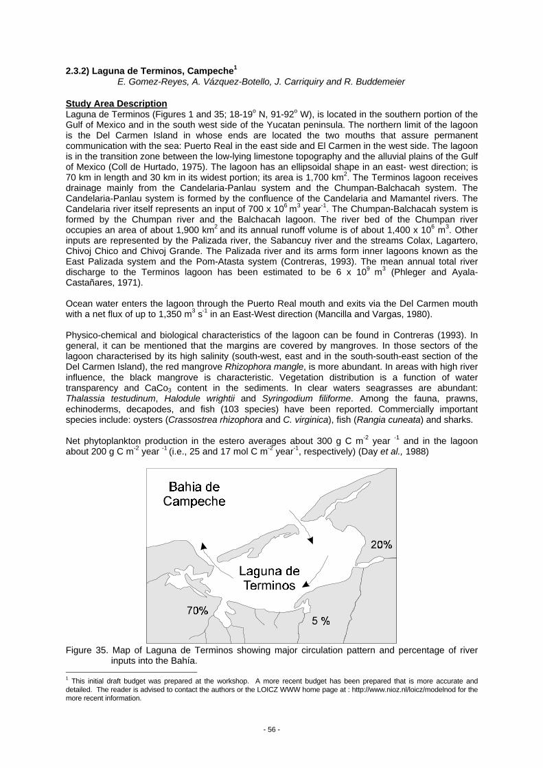
- 56 -
2.3.2) Laguna de Terminos, Campeche1
E. Gomez-Reyes, A. Vázquez-Botello, J. Carriquiry and R. Buddemeier
Study Area DescriptionLaguna de Terminos (Figures 1 and 35; 18-19o N, 91-92o W), is located in the southern portion of theGulf of Mexico and in the south west side of the Yucatan peninsula. The northern limit of the lagoonis the Del Carmen Island in whose ends are located the two mouths that assure permanentcommunication with the sea: Puerto Real in the east side and El Carmen in the west side. The lagoonis in the transition zone between the low-lying limestone topography and the alluvial plains of the Gulfof Mexico (Coll de Hurtado, 1975). The lagoon has an ellipsoidal shape in an east- west direction; is70 km in length and 30 km in its widest portion; its area is 1,700 km2. The Terminos lagoon receivesdrainage mainly from the Candelaria-Panlau system and the Chumpan-Balchacah system. TheCandelaria-Panlau system is formed by the confluence of the Candelaria and Mamantel rivers. TheCandelaria river itself represents an input of 700 x 106 m3 year-1. The Chumpan-Balchacah system isformed by the Chumpan river and the Balchacah lagoon. The river bed of the Chumpan riveroccupies an area of about 1,900 km2 and its annual runoff volume is of about 1,400 x 106 m3. Otherinputs are represented by the Palizada river, the Sabancuy river and the streams Colax, Lagartero,Chivoj Chico and Chivoj Grande. The Palizada river and its arms form inner lagoons known as theEast Palizada system and the Pom-Atasta system (Contreras, 1993). The mean annual total riverdischarge to the Terminos lagoon has been estimated to be 6 x 10⁹ m3 (Phleger and Ayala-Castañares, 1971).
Ocean water enters the lagoon through the Puerto Real mouth and exits via the Del Carmen mouthwith a net flux of up to 1,350 m3 s-1 in an East-West direction (Mancilla and Vargas, 1980).
Physico-chemical and biological characteristics of the lagoon can be found in Contreras (1993). Ingeneral, it can be mentioned that the margins are covered by mangroves. In those sectors of thelagoon characterised by its high salinity (south-west, east and in the south-south-east section of theDel Carmen Island), the red mangrove Rhizophora mangle, is more abundant. In areas with high riverinfluence, the black mangrove is characteristic. Vegetation distribution is a function of watertransparency and CaCo3 content in the sediments. In clear waters seagrasses are abundant:Thalassia testudinum, Halodule wrightii and Syringodium filiforme. Among the fauna, prawns,echinoderms, decapodes, and fish (103 species) have been reported. Commercially importantspecies include: oysters (Crassostrea rhizophora and C. virginica), fish (Rangia cuneata) and sharks.
Net phytoplankton production in the estero averages about 300 g C m-2 year -1 and in the lagoonabout 200 g C m-2 year -1 (i.e., 25 and 17 mol C m-2 year-1, respectively) (Day et al., 1988)
Figure 35. Map of Laguna de Terminos showing major circulation pattern and percentage of riverinputs into the Bahía.
1 This initial draft budget was prepared at the workshop. A more recent budget has been prepared that is more accurate anddetailed. The reader is advised to contact the authors or the LOICZ WWW home page at : http://www.nioz.nl/loicz/modelnod for themore recent information.
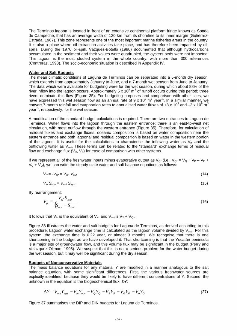
- 57 -
The Terminos lagoon is located in front of an extensive continental platform fringe known as Sondade Campeche, that has an average width of 120 km from its shoreline to its inner margin (Gutiérrez-Estrada, 1967). This zone represents one of the most important marine fisheries areas in the country.It is also a place where oil extraction activities take place, and has therefore been impacted by oil-spills. During the 1976 oil-spill, Vázquez-Botello (1980) documented that although hydrocarbonsaccumulated in the sediment and their values were quadrupled, the oysters beds were not impacted.This lagoon is the most studied system in the whole country, with more than 300 references(Contreras, 1993). The socio-economic situation is described in Appendix IV.
Water and Salt BudgetsThe mean climatic conditions of Laguna de Terminos can be separated into a 5-month dry season,which extends from approximately January to June, and a 7-month wet season from June to January.The data which were available for budgeting were for the wet season, during which about 88% of theriver inflow into the lagoon occurs. Approximately 5 x 10⁹ m3 of runoff occurs during this period; threerivers dominate this flow (Figure 35). For budgeting purposes and comparison with other sites, wehave expressed this wet season flow as an annual rate of 9 x 10⁹ m3 year-1. In a similar manner, weconvert 7-month rainfall and evaporation rates to annualised water fluxes of +3 x 10⁹ and –2 x 10⁹ m3
year-1, respectively, for the wet season.
A modification of the standard budget calculations is required. There are two entrances to Laguna deTerminos. Water flows into the lagoon through the eastern entrance; there is an east-to-west netcirculation, with most outflow through the western entrance (Figure 35). Therefore, for calculation ofresidual fluxes and exchange fluxes, oceanic composition is based on water composition near theeastern entrance and both lagoonal and residual composition is based on water in the western portionof the lagoon. It is useful for the calculations to characterise the inflowing water as Vin and theoutflowing water as Vout. These terms can be related to the “standard” exchange terms of residualflow and exchange flux (VR, VX) for ease of comparison with other systems.
If we represent all of the freshwater inputs minus evaporative output as VQ* (i.e., VQ* = VQ + VP – VE +VG + VO), we can write the steady-state water and salt balance equations as follows:
VR = -VQ* = Vin- Vout (14)
Vin Socn = Vout Ssyst (15)
By rearrangement:
( )systocn
systQin SS
SVV
−= *
(16)
It follows that Vin is the equivalent of VX, and Vout is VX + VQ*.
Figure 36 illustrates the water and salt budgets for Laguna de Terminos, as derived according to thisprocedure. Lagoon water exchange time is calculated as the lagoon volume divided by Vout,. For thissystem, the exchange time is 0.22 year, or almost 3 months. We recognise that there is oneshortcoming in the budget as we have developed it. That shortcoming is that the Yucatán peninsulais a major site of groundwater flow, and this volume flux may be significant in the budget (Perry andVelazquez-Oliman, 1996). We suspect that this is not a serious problem for the water budget duringthe wet season, but it may well be significant during the dry season.
Budgets of Nonconservative MaterialsThe mass balance equations for any material Y are modified in a manner analogous to the saltbalance equation, with some significant differences. First, the various freshwater sources areexplicitly identified, because they would be likely to have different concentrations of Y. Second, theunknown in the equation is the biogeochemical flux, ∆Y:
OoGGPPQQocninsystout YVYVYVYVYVYVY −−−−−=∆ (27)
Figure 37 summarises the DIP and DIN budgets for Laguna de Terminos.

- 58 -
Figure 36. Water and salt budgets for Laguna de Terminos based on data for the wet period (June -January), but expressed as annual rates. See text for details of flux calculations. Systemvolume is in units of 106 m3 . Water fluxes in 106 m3 year-1. Salt fluxes in 106 psu m3
year-1.
P BalanceIt can be seen that the system is net sink for DIP, based on the loading data that we have (∆DIP =146 x 106 mol year-1). It is possible that there are local inputs of DIP associated with agriculturalactivities and not included in the budget, and there might be some groundwater input of DIP. Theseinputs are judged not to be large, at least during the wet season when runoff-derived DIP seemslikely to dominate. In general, DIP flux in groundwater flowing through carbonate terrain is low.
N BalanceThe system is also a net sink for DIN (∆DIN = -1,400 x 106 mol year-1). DIN is often very high ingroundwater, so it seems plausible that this additional DIN source is significant. If there is suchadditional DIN loading, then we have underestimated ∆DIN.
Stoichiometric Calculations of Aspects of Net System MetabolismThese P and N fluxes can be used to calculate nitrogen fixation minus denitrification (nfix-denit)according to the procedures laid out in the previous sections. We calculate (nfix-denit) as thedifference between observed and expected ∆DIN. Expected ∆DIN is ∆DIP multiplied by the N:P ratioof the reacting particulate organic matter. We assume that the appropriate ratio is the Redfield N:Pratio of plankton (16:1). Thus:
(nfix-denit) = -1,400 x 106 – 16 x (-146 x 106) = +936 x 106 mol N year-1
(+0.6 mol N m-2 year-1 over the lagoon area).
Note that the system appears likely to be fixing nitrogen in excess of denitrification.
Similarly, we can estimate net ecosystem metabolism (NEM = p-r) as the negative of thenonconservative DIP flux multiplied by the C:P ratio of the reacting organic matter. If the net reactingmaterial is plankton, the particulate C:P ratio is about 106:1:(p-r) = -106 x (-146 x 106) = +15,476 x 106 mol C year-1 = (+9 mol C m-2 year-1)
The system appears to be net autotrophic.
VQ = 9,000
VE = - 2,000VP = + 3,000
VSystem = 5,000
SSystem = 19 psu
τ = 0.24 years
Vout = 21,176
SOcean = 36 psu
Vin = + 11,176VG = VO = 0
(assumed - probablyincorrect for VG )
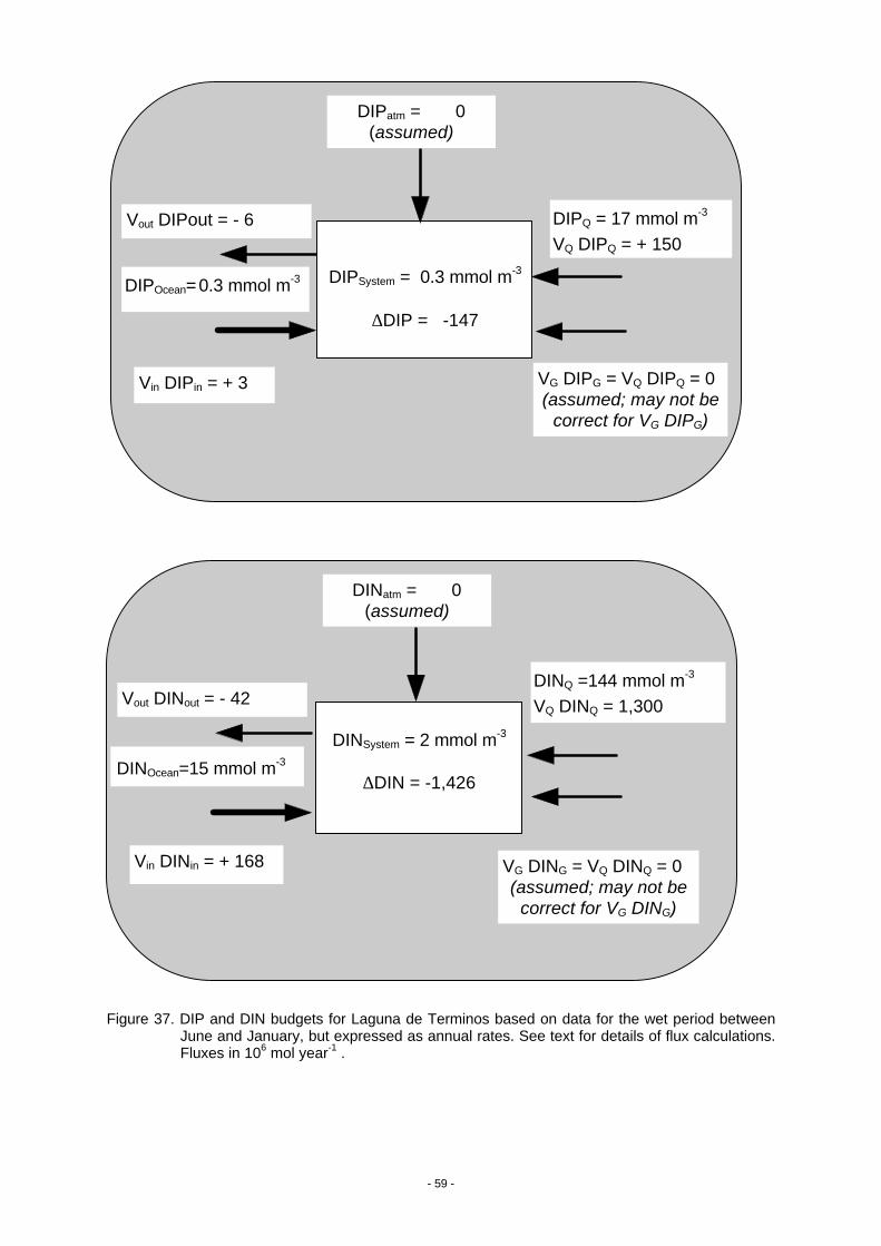
- 59 -
Figure 37. DIP and DIN budgets for Laguna de Terminos based on data for the wet period betweenJune and January, but expressed as annual rates. See text for details of flux calculations.Fluxes in 106 mol year-1 .
DIPQ = 17 mmol m-3
VQ DIPQ = + 150
DIPatm = 0(assumed)
DIPSystem = 0.3 mmol m-3
∆DIP = -147
Vout DIPout = - 6
DIPOcean=0.3 mmol m-3
Vin DIPin = + 3 VG DIPG = VQ DIPQ = 0(assumed; may not be
correct for VG DIPG)
DINQ =144 mmol m-3
VQ DINQ = 1,300
DINatm = 0(assumed)
DINSystem = 2 mmol m-3
∆DIN = -1,426
Vout DINout = - 42
Vin DINin = + 168
DINOcean=15 mmol m-3
VG DING = VQ DINQ = 0(assumed; may not be
correct for VG DING)
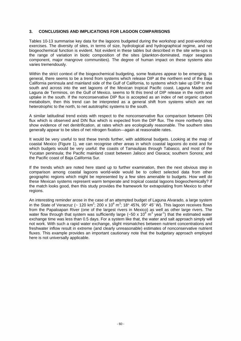
- 60 -
3. CONCLUSIONS AND IMPLICATIONS FOR LAGOON COMPARISONS
Tables 10-13 summarise key data for the lagoons budgeted during the workshop and post-workshopexercises. The diversity of sites, in terms of size, hydrological and hydrographical regime, and netbiogeochemical function is evident. Not evident in these tables but described in the site write-ups isthe range of variation in biotic composition of the sites (plankton-dominated, major seagrasscomponent, major mangrove communities). The degree of human impact on these systems alsovaries tremendously.
Within the strict context of the biogeochemical budgeting, some features appear to be emerging. Ingeneral, there seems to be a trend from systems which release DIP at the northern end of the BajaCalifornia peninsula and mainland side of the Gulf of California, to systems which take up DIP to thesouth and across into the wet lagoons of the Mexican tropical Pacific coast. Laguna Madre andLaguna de Terminos, on the Gulf of Mexico, seems to fit this trend of DIP release in the north anduptake in the south. If the nonconservative DIP flux is accepted as an index of net organic carbonmetabolism, then this trend can be interpreted as a general shift from systems which are netheterotrophic to the north, to net autotrophic systems to the south.
A similar latitudinal trend exists with respect to the nonconservative flux comparison between DINflux which is observed and DIN flux which is expected from the DIP flux. The more northerly sitesshow evidence of net denitrification, at rates which are ecologically reasonable. The southern sitesgenerally appear to be sites of net nitrogen fixation—again at reasonable rates.
It would be very useful to test these trends further, with additional budgets. Looking at the map ofcoastal Mexico (Figure 1), we can recognise other areas in which coastal lagoons do exist and forwhich budgets would be very useful: the coasts of Tamaulipas through Tabasco, and most of theYucatan peninsula; the Pacific mainland coast between Jalisco and Oaxaca; southern Sonora; andthe Pacific coast of Baja California Sur.
If the trends which are noted here stand up to further examination, then the next obvious step incomparison among coastal lagoons world-wide would be to collect selected data from othergeographic regions which might be represented by a few sites amenable to budgets. How well dothese Mexican systems represent warm temperate and tropical coastal lagoons biogeochemically? Ifthe match looks good, then this study provides the framework for extrapolating from Mexico to otherregions.
An interesting reminder arose in the case of an attempted budget of Laguna Alvarado, a large systemin the State of Veracruz (~ 120 km2; 200 x 106 m3; 18° 45’N, 95° 45’ W). This lagoon receives flowsfrom the Papaloapan River (one of the largest rivers in Mexico) as well as other large rivers. Thewater flow through that system was sufficiently large (~50 x 109 m3 year-1) that the estimated waterexchange time was less than 0.5 days. For a system like that, the water and salt approach simply willnot work. With such a rapid water exchange, slight mismatches between nutrient concentrations andfreshwater inflow result in extreme (and clearly unreasonable) estimates of nonconservative nutrientfluxes. This example provides an important cautionary note that the budgetary approach employedhere is not universally applicable.
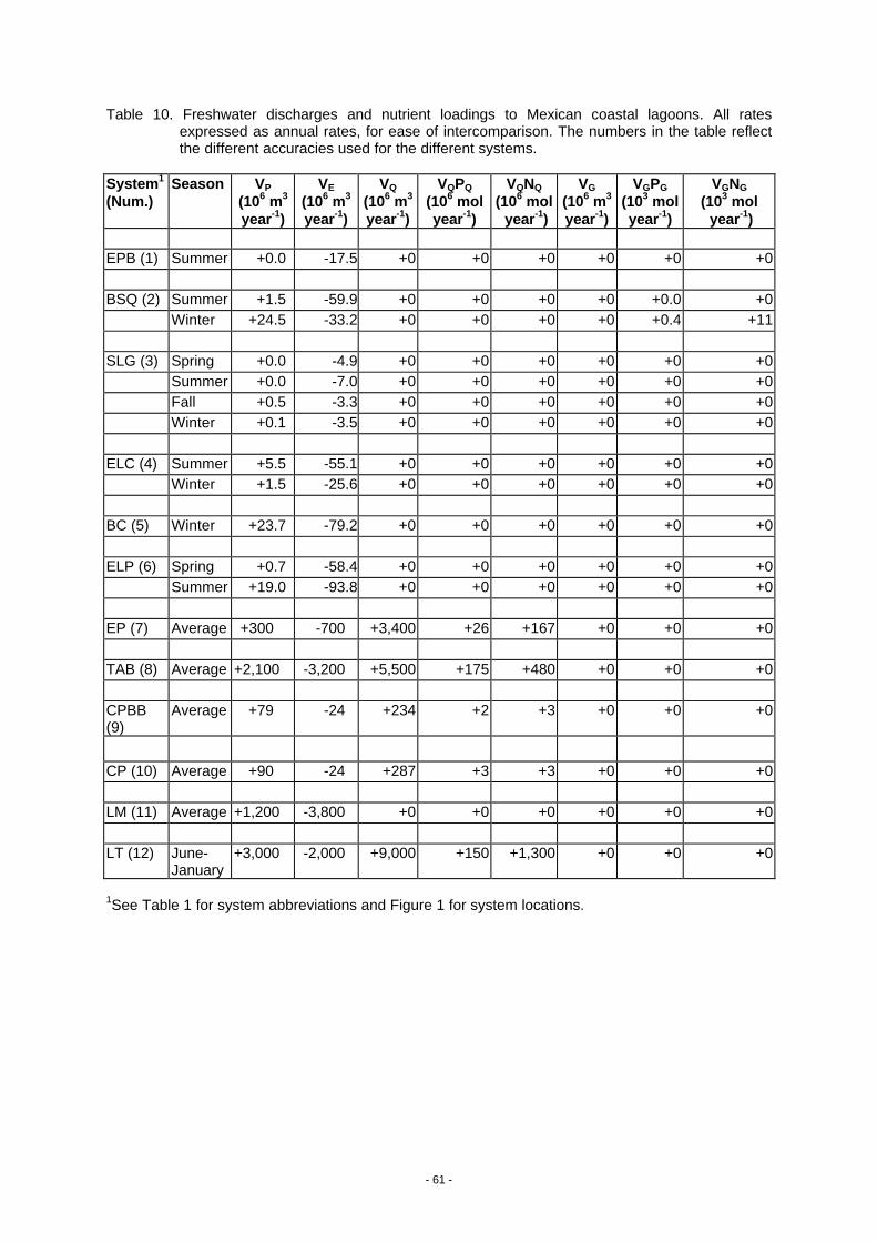
- 61 -
Table 10. Freshwater discharges and nutrient loadings to Mexican coastal lagoons. All ratesexpressed as annual rates, for ease of intercomparison. The numbers in the table reflectthe different accuracies used for the different systems.
System1
(Num.)Season VP
(106 m3
year-1)
VE
(106 m3
year-1)
VQ
(106 m3
year-1)
VQPQ
(106 molyear-1)
VQNQ
(106 mol year-1)
VG
(106 m3
year-1)
VGPG
(103 molyear-1)
VGNG
(103 mol year-1)
EPB (1) Summer +0.0 -17.5 +0 +0 +0 +0 +0 +0
BSQ (2) Summer +1.5 -59.9 +0 +0 +0 +0 +0.0 +0Winter +24.5 -33.2 +0 +0 +0 +0 +0.4 +11
SLG (3) Spring +0.0 -4.9 +0 +0 +0 +0 +0 +0Summer +0.0 -7.0 +0 +0 +0 +0 +0 +0Fall +0.5 -3.3 +0 +0 +0 +0 +0 +0Winter +0.1 -3.5 +0 +0 +0 +0 +0 +0
ELC (4) Summer +5.5 -55.1 +0 +0 +0 +0 +0 +0Winter +1.5 -25.6 +0 +0 +0 +0 +0 +0
BC (5) Winter +23.7 -79.2 +0 +0 +0 +0 +0 +0
ELP (6) Spring +0.7 -58.4 +0 +0 +0 +0 +0 +0Summer +19.0 -93.8 +0 +0 +0 +0 +0 +0
EP (7) Average +300 -700 +3,400 +26 +167 +0 +0 +0
TAB (8) Average +2,100 -3,200 +5,500 +175 +480 +0 +0 +0
CPBB(9)
Average +79 -24 +234 +2 +3 +0 +0 +0
CP (10) Average +90 -24 +287 +3 +3 +0 +0 +0
LM (11) Average +1,200 -3,800 +0 +0 +0 +0 +0 +0
LT (12) June-January
+3,000 -2,000 +9,000 +150 +1,300 +0 +0 +0
1See Table 1 for system abbreviations and Figure 1 for system locations.
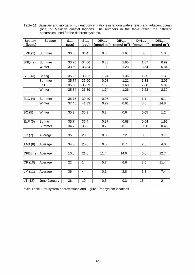
- 62 -
Table 11. Salinities and inorganic nutrient concentrations in lagoon waters (syst) and adjacent ocean(ocn) of Mexican coastal lagoons. The numbers in the table reflect the differentaccuracies used for the different systems.
System1
(Num.)Season Socn
(psu)Ssyst
(psu)DIPocn
(mmol m-3)DIPsyst
(mmol m-3)DINocn
(mmol m-3)DINsyst
(mmol m-3)
EPB (1) Summer 33.6 34.4 0.8 1.6 0.8 1.0
BSQ (2) Summer 33.78 34.66 0.80 1.95 1.87 0.99Winter 33.59 33.84 1.09 1.28 13.54 6.84
SLG (3) Spring 35.26 35.32 1.24 1.36 1.35 1.39Summer 35.74 35.90 0.98 1.21 1.38 2.07Fall 35.50 35.59 1.38 1.60 7.88 5.89Winter 35.34 35.39 1.74 1.26 6.23 2.32
ELC (4) Summer 35.75 39.40 0.95 1.47 6.1 6.1Winter 37.45 41.33 0.27 0.61 8.6 14.8
BC (5) Winter 35.3 35.9 0.3 0.6 0.05 1.2
ELP (6) Spring 35.7 36.4 0.87 0.68 0.64 1.95Summer 34.7 36.2 0.70 0.11 0.50 0.45
EP (7) Average 35 28 0.6 7.2 0.6 3.7
TAB (8) Average 34.0 20.0 0.5 0.7 2.5 4.0
CPBB (9) Average 10.8 21.6 11.4 14.0 6.6 12.7
CP (10) Average 22 14 5.7 6.6 8.6 11.4
LM (11) Average 36 44 0.1 2.8 1.8 7.4
LT (12) June-January 36 19 0.3 0.3 15 2
1See Table 1 for system abbreviations and Figure 1 for system locations
- 63 -
Table 12. Water and salt budget calculations for Mexican coastal lagoons. All rates are expressed asannual rates, for ease of intercomparison. The numbers in the table reflect the differentaccuracies used for the different systems.
System1
(Num.)Season Area
(106 m2)Volume(106 m3)
VR
(106 m year-1)VX
(106 m3 year-1)Exchange
Time (year)
EPB (1) Summer 12 24 +18 +745 .03
BSQ (2) Summer +58 2,271 0.04Winter +8 1,179 0.08Average 42 90
SLG (3) Spring +5 3,005 0.004Summer +7 1,553 0.007Fall +3 1,152 0.009Winter +4 1,288 0.009Average 3 11
ELC (4) Summer +50 511 0.06Winter +24 245 0.12Average 23 32
BC (5) Winter 282 4,553 +55 3,292 1.36
ELP (6) Spring +58 1,471 0.10Summer +75 1,766 0.08Average 45 145
EP (7) Average 460 1,400 -3,000 13,500 0.08
TAB (8) Average 1,600 1,266 -4,645 8,958 0.09
CPBB (9) Average 35 53 -297 434 0.07
CP (10) Average 30 45 -353 1,147 0.013
LM (11) Average 2,000 1,400 +2,600 13,000 0.09
LT (12) June-January 1,700 5,000 -10,000 11,176 0.24
1See Table 1 for system abbreviations and Figure 1 for system locations
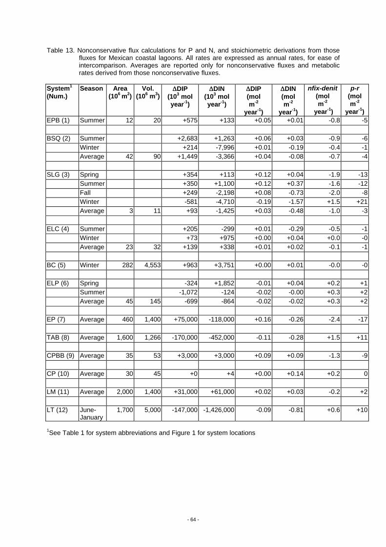
- 64 -
Table 13. Nonconservative flux calculations for P and N, and stoichiometric derivations from thosefluxes for Mexican coastal lagoons. All rates are expressed as annual rates, for ease ofintercomparison. Averages are reported only for nonconservative fluxes and metabolicrates derived from those nonconservative fluxes.
System1
(Num.)Season Area
(106 m2)Vol.
(106 m3)∆∆DIP
(103 molyear-1)
∆∆DIN(103 molyear-1)
∆∆DIP(molm-2
year-1)
∆∆DIN(molm-2
year-1)
nfix-denit(molm-2
year-1)
p-r(molm-2
year-1)EPB (1) Summer 12 20 +575 +133 +0.05 +0.01 -0.8 -5
BSQ (2) Summer +2,683 +1,263 +0.06 +0.03 -0.9 -6Winter +214 -7,996 +0.01 -0.19 -0.4 -1Average 42 90 +1,449 -3,366 +0.04 -0.08 -0.7 -4
SLG (3) Spring +354 +113 +0.12 +0.04 -1.9 -13Summer +350 +1,100 +0.12 +0.37 -1.6 -12Fall +249 -2,198 +0.08 -0.73 -2.0 -8Winter -581 -4,710 -0.19 -1.57 +1.5 +21Average 3 11 +93 -1,425 +0.03 -0.48 -1.0 -3
ELC (4) Summer +205 -299 +0.01 -0.29 -0.5 -1Winter +73 +975 +0.00 +0.04 +0.0 -0Average 23 32 +139 +338 +0.01 +0.02 -0.1 -1
BC (5) Winter 282 4,553 +963 +3,751 +0.00 +0.01 -0.0 -0
ELP (6) Spring -324 +1,852 -0.01 +0.04 +0.2 +1Summer -1,072 -124 -0.02 -0.00 +0.3 +2Average 45 145 -699 -864 -0.02 -0.02 +0.3 +2
EP (7) Average 460 1,400 +75,000 -118,000 +0.16 -0.26 -2.4 -17
TAB (8) Average 1,600 1,266 -170,000 -452,000 -0.11 -0.28 +1.5 +11
CPBB (9) Average 35 53 +3,000 +3,000 +0.09 +0.09 -1.3 -9
CP (10) Average 30 45 +0 +4 +0.00 +0.14 +0.2 0
LM (11) Average 2,000 1,400 +31,000 +61,000 +0.02 +0.03 -0.2 +2
LT (12) June-January
1,700 5,000 -147,000 -1,426,000 -0.09 -0.81 +0.6 +10
1See Table 1 for system abbreviations and Figure 1 for system locations
- 65 -
4. REFERENCES
Acosta-Ruiz, M. and S. Alvarez-Borrego. 1974. Distribución superficial de algunos parámetroshidrológicos y físico-químicos en el Estero de Punta Banda, B.C. en otoño e invierno.Ciencias Marinas, 1: 16-45.
Alvarez-Borrego, S., R. Lara-Lara and M.J. Acosta-Ruiz. 1977. Parametros relacionados con laproductividad organica primaria en dos antiestuarios de Baja California. Ciencias Marinas 4:1-12.
Botello-Ruvalcaba M. and J. Valdez-Holguín. 1990. Productividad primaria en el Estero la Cruz,Sonora, México. Memorias del IV congreso de la Sociedad Mexicana de Plantología.Mazatlán, Sinaloa, México.
Botello-Ruvalcaba, M. 1992. Caracterización de las condiciones hidrológicas y biomasa delfitoplancton durante otoño, en un sistema lagunar de la región central del Golfo deCalifornia. Memorias del IX Congreso Nacional de Oceanografía. Veracruz, Veracruz,México.
Botello-Ruvalcaba, M. 1996. Nutrients and primary productivity in relation to the potential foreutrophication and management, in the central region of the Gulf of California, Mexico.Estuarine and Coastal Science Association 26 and Estuarine Research Federation 96 JointSymposium. Middleburg, The Netherlands.
Castañeda, O. and F. Contreras (compilers). 1995. Ecosistemas Costeros Mexicanos. ComisionNacional Para el Conocimiento y Uso de la Biodiversidad. Universidad AutonónaMetropolitana Unidad Iztapalapa, (CD-ROM).
Castañeda, O., and F. Contreras. 1997. Addendum Serie Bibliografia comentada sobre ecosistemascosteros mexicanos. Universidad Autónoma Metropolitana, Mexico. 225 p.
Castro-Longoria R., J. Grijalba-Chon, A. Meling-López, P. Ortega-Romero, J. Valdez-Holguin and A.Villalba-Atondo. 1989. Aportación de materia orgánica por productores primarios en lalaguna costera La Cruz, Sonora. Informe técnico final del proyecto UNISON-CONACyTclave ICCNXNA-031345. Departamento de Investigaciones Científicas y tecnológicas de laUniversidad de Sonora, Hermosillo, Sonora, México.
Céliz-Ceseña, R.,1975. Distribución superficial de algunos parámetros hidrológicos, físicos yquímicos en el estero de Punta Banda, B. C. durante primavera y verano. U.A.B.C. TesisLicenciatura.
Celis-Ceseña, R. and S. Alvarez-Borrego. 1975. Distribución superficial de algunos parámetroshidrológicos, físicos y químicos en el Estero de Punta Banda, B.C. en primavera y verano.Ciencias Marinas, 2: 98-105.
Cervantes-Duarte, R. 1981. Distribución de nutrientes en la Ensenada de La Paz, B.C.S., durante elperíodo de primavera-verano de 1981. Professional Thesis. Universidad Autónoma de BajaCalifornia. 119 pp.
Coll de Hurtado, A., 1975. El sureste de Campeche y sus recursos naturales. Inst. Geogr. UNAM.Serie Cuadernos. 85 pp.
Contreras, F. 1985. Las Lagunas Costeras Mexicanas. Centro de Ecodesarrollo, Secretaria dePesca, Mexico. 253 pp.
Contreras, F. 1993. Ecosistemas Costeros Mexicanos. Comision Nacional Para el Conocimiento yUso de la Biodiversidad. Universidad Autonóna Metropolitana Unidad Iztapalapa, 415 pp.
Contreras, F. and L.M. Zabalegui. 1988. Aprovechamiento del Litoral Mexicano. Centro deEcodesarrollo, Secretaria de Pesca, Mexico. 128 pp.
- 66 -
Day, J.W., Jr., F. Ley-Lou, C.J. Madden, R.L. Wetzel and A. Machado., 1988. Aquatic primaryproductivity in Terminos Lagoon, Chap. 13: 221-236. in: Yan~ez-Arancibia, A. and J.W. Day,Jr. (Eds.). Ecology of Coastal Ecosystems in the Southern Gulf of Mexico: The TerminosLagoon Region. Inst. Cienc. del Mar y Limnol. UNAM, Coast. Ecol. Inst. LSU. EditorialUniversitaria, Mexico, D.F.
Estado de Tamaulipas, G. del. 1996. Canal Intracostero Tamaulipeco. 80 pp.
Gilmartin, M. and N. Revelante. 1978. The phytoplankton characteristics of the barrier island lagoonsof the Gulf of California. Estuarine And Coastal Marine Science, 7: 29-47.
Gordon, D.C. Jr., P.R. Boudreau , K.H. Mann, J.-E. Ong, W.L. Silvert, S.V. Smith, G. Wattayakorn,F. Wulff and T. Yanagi. 1996. LOICZ Biogeochemical Modelling Guidelines. LOICZ Reports& Studies No. 5. Second Edition, vi +96 pp. LOICZ, Texel, The Netherlands.
Gutierrez-Estrada, M., 1977. Resultados preliminares del estudio geológico de la Isla del Carmen.Res. III Congr. Nal. Oceanogr.
Ibarra-Obando, S.E. and A. Escofet. 1987. Industrial development effects on the ecology of a PacificMexican estuary. Environmental Conservation, 14: 135-141.
Ibarra-Obando, S.E. and M. Poumian-Tapia. 1992. The saltmarsh vegetation of Punta BandaEstuary, Baja California, Mexico. in: Seeliger, U. (ed.). Coastal Plant Communities of LatinAmerica. Academic Press, San Diego: 201-211.
Ibarra-Obando, S.E. and M. Poumian-Tapia. 1991. The effect of tidal exclusion on salt marshvegetation in Baja California, México. Wetlands Ecology and Management, 1: 131-148.
Ibarra-Obando, S. and R. Huerta-Tamayo. 1987. Blade production of Zostera marina (L). during thesummer-autumn period on the Pacific coast of Mexico. Aquatic Botany 28: 301-315.
INEGI. 1994. Instituto Nacional de Estadistica, Geografia e Informatica. Estadisticas del MedioAmbiente. Mexico 447 pp.
Lankford, R.R. 1977. Coastal lagoons of Mexico: Their origin and classification. pp. 182-215 In M.Wiley (ed.) Estuarine Processes. Academic, New York.
Lechuga-Devéze, C.H. 1994. Shift of acetone extracted pigments due to unknown naturalphytoplankton populations from Conception Bay, Gulf of California. Bulletin of MarineScience, 55: 248-255.
Lechuga-Devéze, C.H., Ma.-L. Morquecho-Escamilla, A. Reyes-Salinas and A. Reyes-Hernández.1997. Environmental natural disturbances at Bahía Concepción, Gulf of California. AquaticEcosystems of México Symposium. 8-10 March, 1997. México City.
Lechuga-Devéze, C.H., J. Bustillos-Guzmán, Ma.-T Barreiro-Guémez and D. López-Cortés. 1990.Oscilaciones semi-diurnas, diarias y estacionales de variables físicas en la Ensenada de LaPaz, B.C.S. Investicaciones del Mar. CICIMAR, 5 : 1-9
Lechuga-Devéze, C.H., J. García-Pámanes and J. Bustillos-Guzmán. 1986. Ecological conditions ofa coastal lagoon on the Gulf of California west coast. Turbidity and chlorophyll a. CienciasMarinas, 12: 19-31.
Mancilla, P.M. and F.M. Vargas. 1980. Los primeros estudios sobre la circulación y el flujo neto deagua a través de la laguna de Términos, Campeche, México. An. Centro Cienc del Mar yLimnol. UNAM, 7(2): 1-12.
- 67 -
Martínez-Inostros, M. 1994. Caracterización de oxígeno, salinidad, temperatura y nutrientes antes ydespues de una temporada de lluvia. (Septiembre 1992-Marzo 1993) en el Estero de PuntaBanda, Baja California. Tesis de Licenciatura. Ciencias Marinas. Universidad Autónoma deBaja California.
Mendoza-Espinosa, L.G. 1994. Variación diurna y estacional de variables hidrológicas y clorofila aen Bahía Willard, Golfo de California. B.S. Thesis. Facultad de Ciencias Marinas.Universidad Autónoma de Baja California. 52 pp.
Mee, D.L. 1977. Coastal lagoons. Pp. 441-490 In Riley and Chester (eds.) Chemical Oceanographyv. 7. Academic, New York.
Merino-Paredes, M. 1987. Variación estacional de la producción primaria, clorofila y seston en Bahía Willard,costa oeste del Golfo de California. B.S. Thesis. Facultad de Ciencias Marinas: 68 pp.
Millán-Núñez, E., Ortiz-Cortez, F. and Alvarez-Borrego, S., 1981. Variabilidad temporal y espacial denutrientes y fitoplancton en una laguna costera, a finales de verano. Ciencias Marinas.7:103-125
Morquecho-Escamilla, Ma.-L. and I. Murillo-Murillo. 1995. Parámetros físicoquimicos y biomasafitoplanctónica en Bahía de La Paz y Bahía Magdalena, B.C.S. Technical Report. CIBNOR.36 pp.
Pernetta, J.C. and J. Milliman. 1995. Land-Ocean Interactions in the Coastal Zone ImplementationPlan. IGBP Report No. 33, Stockholm. 215 pp.
Phleger, F.B. and A. Ayala-Castañares. 1971. Processes and history of Terminos lagoon, Mexico.Bulletin of the American Association of Petroleum Geologists, 55: 2130-2140.
Pritchard, D.W. 1967. What is an estuary? Physical viewpoint. in: Lauff G. (ed.). Estuaries, 83:3-5.
Pritchard, D.W., R. de la. Paz-Vela, H. Cabrera-Muro, S. Farreras-Sanz and E. Morales. 1978.Hidrografía física del estero de Punta Banda, parte I: Análisis de datos. Ciencias Marinas, 5:1-23.
Redfield, A.C. 1934. On the proportions of organic derivatives in sea water and their relation to thecomposition of plankton. James Johnstone Memorial Volume, Liverpool. 177-192 pp.
Reyes-Salinas. 1994. Relación entre estructura hidrográfica y la abundancia, distribución y origen dediferentes expresiones de biomasa del seston orgánico en Bahía Concepción, Golfo deCalifornia. Professional Thesis, Universidad Nacional Autónoma de México. 53 pp.
Smith, S.V., and J.T. Hollibaugh. 1993. Coastal metabolism and the oceanic organic carbon balance.Reviews of Geophysics. 31: 75-89.
Segovia-Zavala, J.A., Rivera-Duarte, I., del Valle-Villorín, F.J., 1988. Efectos de desechos orgánicosen las zonas adyacentes a los efluentes en Bahía de Todos Santos: Nutrientes. CienciasMarinas. 14:81-94
Valdez-Holguín, J. 1994. Daily variations of temperature, salinity, dissolves oxygen and chorophyll-a,in a hypersaline lagoon of the Gulf of California. Ciencias Marinas. 20:123-137. México.
Valdez-Holguín, J. and Martínez Cordova. 1993. Variabilidad de algunos parámetros fisicoquímicos yproductividad primaria en la laguna La Cruz, Sonora, México. Revista de Biología Tropical.41 :161-179.
Vázquez-Botello, A., 1980. Cuantificación de un derrame petrolero ocurrido en la laguna deTérminos, Campeche, Mexico. 1976. An Centro Cienc. Del Mar y Limnol. UNAM, 7: 169-176.
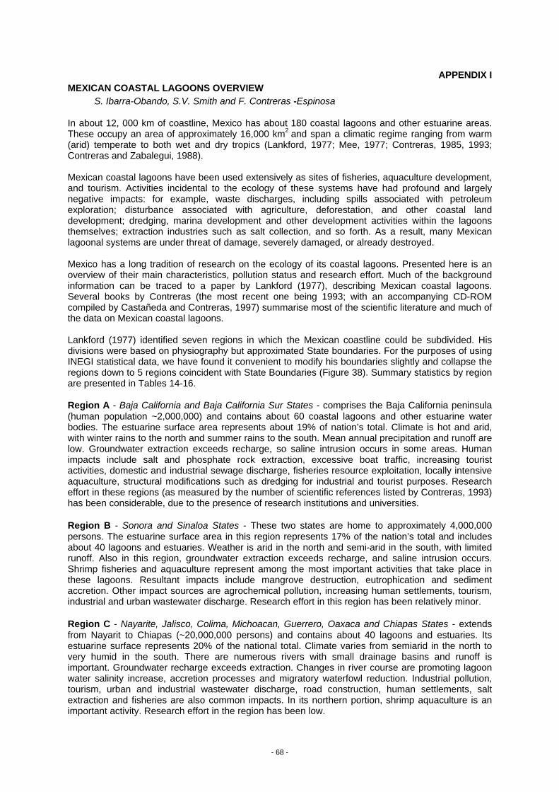
- 68 -
APPENDIX IMEXICAN COASTAL LAGOONS OVERVIEW
S. Ibarra-Obando, S.V. Smith and F. Contreras -Espinosa
In about 12, 000 km of coastline, Mexico has about 180 coastal lagoons and other estuarine areas.These occupy an area of approximately 16,000 km2 and span a climatic regime ranging from warm(arid) temperate to both wet and dry tropics (Lankford, 1977; Mee, 1977; Contreras, 1985, 1993;Contreras and Zabalegui, 1988).
Mexican coastal lagoons have been used extensively as sites of fisheries, aquaculture development,and tourism. Activities incidental to the ecology of these systems have had profound and largelynegative impacts: for example, waste discharges, including spills associated with petroleumexploration; disturbance associated with agriculture, deforestation, and other coastal landdevelopment; dredging, marina development and other development activities within the lagoonsthemselves; extraction industries such as salt collection, and so forth. As a result, many Mexicanlagoonal systems are under threat of damage, severely damaged, or already destroyed.
Mexico has a long tradition of research on the ecology of its coastal lagoons. Presented here is anoverview of their main characteristics, pollution status and research effort. Much of the backgroundinformation can be traced to a paper by Lankford (1977), describing Mexican coastal lagoons.Several books by Contreras (the most recent one being 1993; with an accompanying CD-ROMcompiled by Castañeda and Contreras, 1997) summarise most of the scientific literature and much ofthe data on Mexican coastal lagoons.
Lankford (1977) identified seven regions in which the Mexican coastline could be subdivided. Hisdivisions were based on physiography but approximated State boundaries. For the purposes of usingINEGI statistical data, we have found it convenient to modify his boundaries slightly and collapse theregions down to 5 regions coincident with State Boundaries (Figure 38). Summary statistics by regionare presented in Tables 14-16.
Region A - Baja California and Baja California Sur States - comprises the Baja California peninsula(human population ~2,000,000) and contains about 60 coastal lagoons and other estuarine waterbodies. The estuarine surface area represents about 19% of nation’s total. Climate is hot and arid,with winter rains to the north and summer rains to the south. Mean annual precipitation and runoff arelow. Groundwater extraction exceeds recharge, so saline intrusion occurs in some areas. Humanimpacts include salt and phosphate rock extraction, excessive boat traffic, increasing touristactivities, domestic and industrial sewage discharge, fisheries resource exploitation, locally intensiveaquaculture, structural modifications such as dredging for industrial and tourist purposes. Researcheffort in these regions (as measured by the number of scientific references listed by Contreras, 1993)has been considerable, due to the presence of research institutions and universities.
Region B - Sonora and Sinaloa States - These two states are home to approximately 4,000,000persons. The estuarine surface area in this region represents 17% of the nation’s total and includesabout 40 lagoons and estuaries. Weather is arid in the north and semi-arid in the south, with limitedrunoff. Also in this region, groundwater extraction exceeds recharge, and saline intrusion occurs.Shrimp fisheries and aquaculture represent among the most important activities that take place inthese lagoons. Resultant impacts include mangrove destruction, eutrophication and sedimentaccretion. Other impact sources are agrochemical pollution, increasing human settlements, tourism,industrial and urban wastewater discharge. Research effort in this region has been relatively minor.
Region C - Nayarite, Jalisco, Colima, Michoacan, Guerrero, Oaxaca and Chiapas States - extendsfrom Nayarit to Chiapas (~20,000,000 persons) and contains about 40 lagoons and estuaries. Itsestuarine surface represents 20% of the national total. Climate varies from semiarid in the north tovery humid in the south. There are numerous rivers with small drainage basins and runoff isimportant. Groundwater recharge exceeds extraction. Changes in river course are promoting lagoonwater salinity increase, accretion processes and migratory waterfowl reduction. Industrial pollution,tourism, urban and industrial wastewater discharge, road construction, human settlements, saltextraction and fisheries are also common impacts. In its northern portion, shrimp aquaculture is animportant activity. Research effort in the region has been low.
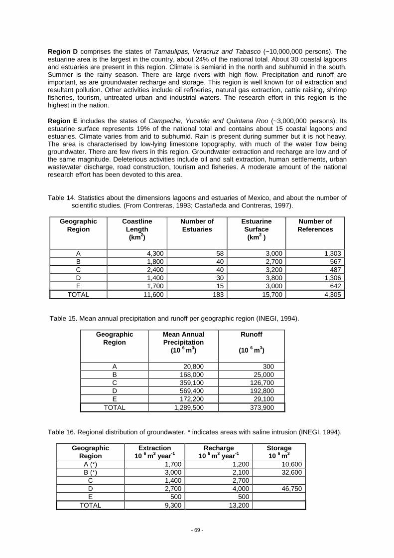
- 69 -
Region D comprises the states of Tamaulipas, Veracruz and Tabasco (~10,000,000 persons). Theestuarine area is the largest in the country, about 24% of the national total. About 30 coastal lagoonsand estuaries are present in this region. Climate is semiarid in the north and subhumid in the south.Summer is the rainy season. There are large rivers with high flow. Precipitation and runoff areimportant, as are groundwater recharge and storage. This region is well known for oil extraction andresultant pollution. Other activities include oil refineries, natural gas extraction, cattle raising, shrimpfisheries, tourism, untreated urban and industrial waters. The research effort in this region is thehighest in the nation.
Region E includes the states of Campeche, Yucatán and Quintana Roo (~3,000,000 persons). Itsestuarine surface represents 19% of the national total and contains about 15 coastal lagoons andestuaries. Climate varies from arid to subhumid. Rain is present during summer but it is not heavy.The area is characterised by low-lying limestone topography, with much of the water flow beinggroundwater. There are few rivers in this region. Groundwater extraction and recharge are low and ofthe same magnitude. Deleterious activities include oil and salt extraction, human settlements, urbanwastewater discharge, road construction, tourism and fisheries. A moderate amount of the nationalresearch effort has been devoted to this area.
Table 14. Statistics about the dimensions lagoons and estuaries of Mexico, and about the number ofscientific studies. (From Contreras, 1993; Castañeda and Contreras, 1997).
GeographicRegion
CoastlineLength(km2)
Number ofEstuaries
EstuarineSurface(km2 )
Number ofReferences
A 4,300 58 3,000 1,303B 1,800 40 2,700 567C 2,400 40 3,200 487D 1,400 30 3,800 1,306E 1,700 15 3,000 642
TOTAL 11,600 183 15,700 4,305
Table 15. Mean annual precipitation and runoff per geographic region (INEGI, 1994).
GeographicRegion
Mean AnnualPrecipitation
(10 6 m3)
Runoff
(10 6 m3)
A 20,800 300B 168,000 25,000C 359,100 126,700D 569,400 192,800E 172,200 29,100
TOTAL 1,289,500 373,900
Table 16. Regional distribution of groundwater. * indicates areas with saline intrusion (INEGI, 1994).
GeographicRegion
Extraction10 6 m3 year-1
Recharge10 6 m3 year-1
Storage10 6 m3
A (*) 1,700 1,200 10,600B (*) 3,000 2,100 32,600
C 1,400 2,700D 2,700 4,000 46,750E 500 500
TOTAL 9,300 13,200
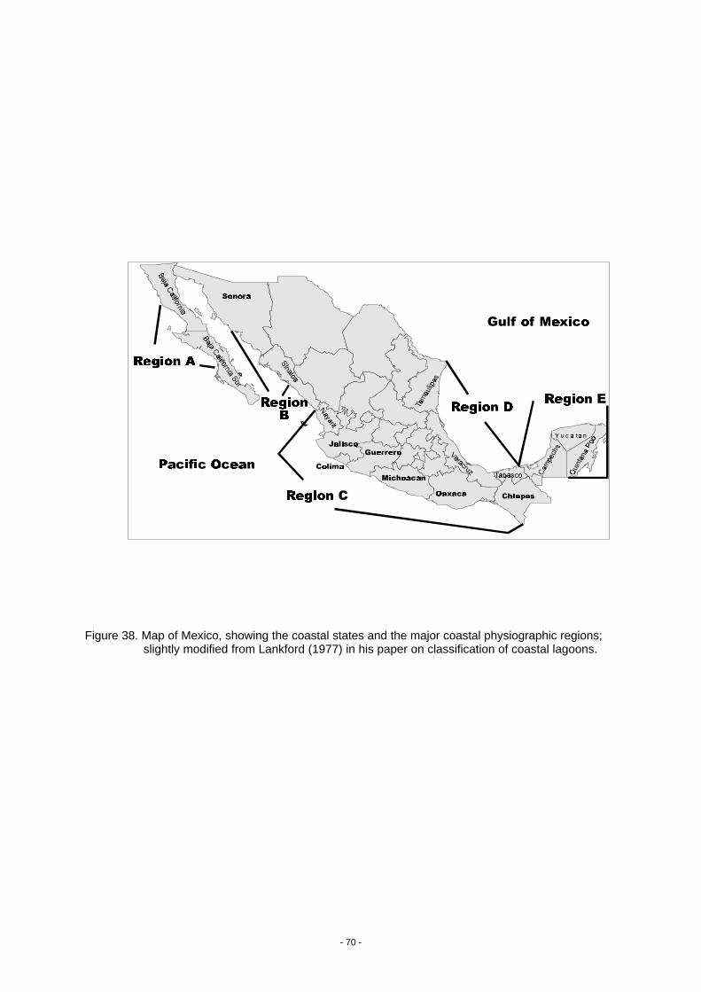
- 70 -
Figure 38. Map of Mexico, showing the coastal states and the major coastal physiographic regions;slightly modified from Lankford (1977) in his paper on classification of coastal lagoons.
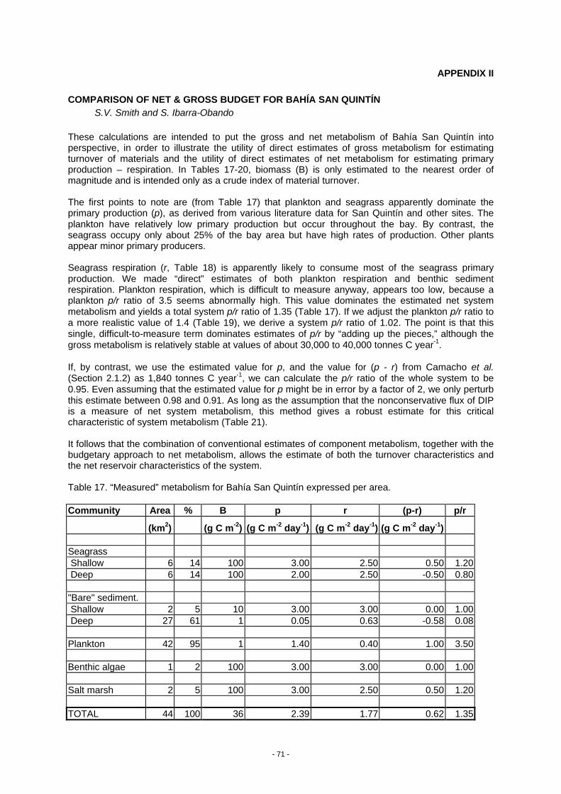
- 71 -
APPENDIX II
COMPARISON OF NET & GROSS BUDGET FOR BAHÍA SAN QUINTÍNS.V. Smith and S. Ibarra-Obando
These calculations are intended to put the gross and net metabolism of Bahía San Quintín intoperspective, in order to illustrate the utility of direct estimates of gross metabolism for estimatingturnover of materials and the utility of direct estimates of net metabolism for estimating primaryproduction – respiration. In Tables 17-20, biomass (B) is only estimated to the nearest order ofmagnitude and is intended only as a crude index of material turnover.
The first points to note are (from Table 17) that plankton and seagrass apparently dominate theprimary production (p), as derived from various literature data for San Quintín and other sites. Theplankton have relatively low primary production but occur throughout the bay. By contrast, theseagrass occupy only about 25% of the bay area but have high rates of production. Other plantsappear minor primary producers.
Seagrass respiration (r, Table 18) is apparently likely to consume most of the seagrass primaryproduction. We made “direct” estimates of both plankton respiration and benthic sedimentrespiration. Plankton respiration, which is difficult to measure anyway, appears too low, because aplankton p/r ratio of 3.5 seems abnormally high. This value dominates the estimated net systemmetabolism and yields a total system p/r ratio of 1.35 (Table 17). If we adjust the plankton p/r ratio toa more realistic value of 1.4 (Table 19), we derive a system p/r ratio of 1.02. The point is that thissingle, difficult-to-measure term dominates estimates of p/r by “adding up the pieces,” although thegross metabolism is relatively stable at values of about 30,000 to 40,000 tonnes C year-1.
If, by contrast, we use the estimated value for p, and the value for (p - r) from Camacho et al.(Section 2.1.2) as 1,840 tonnes C year-1, we can calculate the p/r ratio of the whole system to be0.95. Even assuming that the estimated value for p might be in error by a factor of 2, we only perturbthis estimate between 0.98 and 0.91. As long as the assumption that the nonconservative flux of DIPis a measure of net system metabolism, this method gives a robust estimate for this criticalcharacteristic of system metabolism (Table 21).
It follows that the combination of conventional estimates of component metabolism, together with thebudgetary approach to net metabolism, allows the estimate of both the turnover characteristics andthe net reservoir characteristics of the system.
Table 17. “Measured” metabolism for Bahía San Quintín expressed per area.
Community Area % B p r (p-r) p/r
(km2) (g C m-2) (g C m-2 day-1) (g C m-2 day-1) (g C m-2 day-1)
Seagrass Shallow 6 14 100 3.00 2.50 0.50 1.20 Deep 6 14 100 2.00 2.50 -0.50 0.80
"Bare" sediment. Shallow 2 5 10 3.00 3.00 0.00 1.00 Deep 27 61 1 0.05 0.63 -0.58 0.08
Plankton 42 95 1 1.40 0.40 1.00 3.50
Benthic algae 1 2 100 3.00 3.00 0.00 1.00
Salt marsh 2 5 100 3.00 2.50 0.50 1.20
TOTAL 44 100 36 2.39 1.77 0.62 1.35
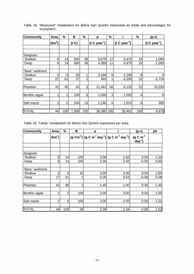
- 72 -
Table 18. “Measured” metabolism for Bahía San Quintín expressed as totals and percentages forecosystem.
Community Area % B % p % r % (p-r)
(km2) (t C) (t C year-1) (t C year-1) (t C year-1)
Seagrass Shallow 6 14 600 38 6,570 17 5,475 19 1,095 Deep 6 14 600 38 4,380 11 5,475 19 -1,095
"Bare" sediment Shallow 2 5 20 1 2,190 6 2,190 8 0 Deep 27 61 27 2 493 1 6,209 22 -5,716
Plankton 42 95 42 3 21,462 56 6,132 22 15,330
Benthic algae 1 2 100 6 1,095 3 1,095 4 0
Salt marsh 2 5 200 13 2,190 6 1,825 6 365
TOTAL 44 100 1,589 100 38,380 100 28,401 100 9,979
Table 19. “Likely” metabolism for Bahía San Quintín expressed per area.
Community Area % B p r (p-r) p/r
(km2) (g Cm-2) (g C m-2 day-1) (g C m-2 day-1) (g C m-2
day-1)
Seagrass Shallow 6 14 100 3.00 2.50 0.50 1.20 Deep 6 14 100 2.00 2.50 -0.50 0.80
"Bare" sediment. Shallow 2 5 10 3.00 3.00 0.00 1.00 Deep 27 61 1 0.05 0.63 -0.58 0.08
Plankton 42 95 1 1.40 1.00 0.40 1.40
Benthic algae 1 2 100 3.00 3.00 0.00 1.00
Salt marsh 2 5 100 3.00 2.50 0.50 1.20
TOTAL 44 100 36 2.39 2.34 0.05 1.02
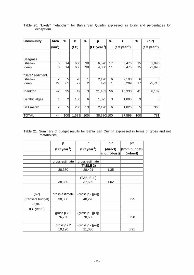
- 73 -
Table 20. “Likely” metabolism for Bahía San Quintín expressed as totals and percentages forecosystem.
Community Area % B % p % r % (p-r)
(km2) (t C) (t C year-1) (t C year-1) (t C year-1)
Seagrass shallow 6 14 600 38 6,570 17 5,475 15 1,095 deep 6 14 600 38 4,380 11 5,475 15 -1,095
"Bare" sediment. shallow 2 5 20 1 2,190 6 2,190 6 0 deep 27 61 27 2 493 1 6,209 17 -5,716
Plankton 42 95 42 3 21,462 56 15,330 41 6,132
Benthic algae 1 2 100 6 1,095 3 1,095 3 0
Salt marsh 2 5 200 13 2,190 6 1,825 5 365
TOTAL 44 100 1,589 100 38,380 100 37,599 100 781
Table 21. Summary of budget results for Bahía San Quintín expressed in terms of gross and netmetabolism.
p r p/r p/r
(t C year-1) (t C year-1) (direct) (from budget)(not robust) (robust)
gross estimate gross estimate(TABLE 3)
38,380 28,401 1.35
(TABLE 4.)38,380 37,599 1.02
(p-r) gross estimate (gross p - [p-r])(transect budget) 38,380 40,220 0.95
-1,840(t C year-1)
gross p x 2 (gross p - [p-r])76,760 78,600 0.98
gross p / 2 (gross p - [p-r])19,190 21,030 0.91
- 74 -
APPENDIX III
ECOLOGICAL SERVICES AND SOCIO-ECONOMIC SUSTAINABILITY -A case study: Bahía San Quintín
IntroductionThe overall aim of IGBP is “to describe and understand the interactive physical, chemical andbiological processes that regulate the total Earth system, the unique environment that it provides forlife, the changes that are occurring in the system and the manner in which they are influenced byhuman actions” (Pernetta and Milliman, 1995).
LOICZ is that component of the IGBP which focuses on the area of the earth’s surface where land,ocean and atmosphere meet and interact. The overall goal of this project is to determine at regionaland global scales: the nature of that dynamic interaction; how changes in various components of theEarth system are affecting coastal zones and altering their role in global cycles; to assess how futurechanges in these areas will affect their use by people; and to provide a sound scientific basis forfuture integrated management of coastal areas on a sustainable basis (Pernetta and Milliman, 1995).
One of the ways in which the LOICZ project is achieving the required integration to reach its goal isbudgeting water, C, N and P in the coastal zone. Human populations and economic activities alter C,N, P, water, and sediment inventories, and their fluxes within and through the coastal zone. Thesesame fluxes and inventories represent and control the processes that define the living resources --terrestrial, aquatic and marine -- that provide direct and indirect economic goods and services tohumankind. This link between natural science and socio-economics has yet to be successfullyaddressed by any of the IGBP core project elements. For this reason we have decided to undertakean integrative study using Bahía San Quintín as a study case.
The San Quintín system is represented by the San Simon valley and a coastal lagoon known asBahía San Quintín (Figure 5). This system is located in the Baja California Peninsula (30o N); itswatershed covers an area of approximately 2,000 km2, and the surface area of the Bay itself is about40 km2. The system is very arid, with an average annual rainfall of approximately 200 mm year-1 andpan evaporation of 1,500 mm year-1 near the coast. There is no significant surface runoff from landinto the bay except during major storms. Groundwater represents the only freshwater source and isheavily exploited in order to sustain agriculture. Agriculture (dominated by tomato growing)represents the most important economic activity in the region, providing jobs for local people andmigrants coming from the southern part of Mexico (mainly Oaxaca).
This agricultural activity is far more intensive than can be sustained naturally, and virtually all of theproduce is exported. Water use is about 12 x 106 m3 year-1 greater than the recharge of 30 x 106 m3
year-1, and the aquifer is being drawn down by about 3% per year. This is causing saline intrusionalong the coast, where the human population lives and relies on the groundwater for domestic,municipal and industrial water supplies. Further, this activity is relying heavily on the import ofinorganic fertilisers. Some of the fertiliser nutrient elements enter the aquifer, further contaminatingthe remaining fresh water.
The human population of the region is readily divided into two groups: a permanent population ofabout 25,000 persons, most of whom live in 3 towns in the San Quintín valley, and about that samenumber of migrant labourers, who are there an average of about half the year and who mostly live incamps. There is no sewage treatment for the wastes from either of these groups, so their dischargelargely percolates into the top of the aquifer.
The marine part of the system, known as Bahía San Quintín, is a hypersaline coastal lagoon; its areaconsists of two sub-basins: Bahía Falsa (west) and Bahía San Quintín (east) (Figure 5). The bay hasa permanent mouth and exchanges nutrients and organic materials with the coastal ocean. Thesystem is a net exporter of dissolved inorganic phosphorus, apparently derived from thedecomposition of particulate organic matter exported from outside the system.

- 75 -
Two economic activities are significant in extracting living resources from the marine system, butboth are sustained naturally. The first of these is an artesanal harvesting of the natural population ofclams. Second, since about 1970 Bahía Falsa has been used for oyster culture, with this being themost important economic activity for the marine part of the system. There is some question as towhether these two extractive industries compete with one another. Other relevant activities usinginclude tourism, especially sport fishing (outside the bay) and duck hunting.

- 76 -
APPENDIX IV
SOCIO-ECONOMIC SITUATION OF LAGUNA DE TERMINOSA. Vázquez-Botello
GeneralThe Mexican State of Campeche covers 2.6% of the total land surface of Mexico; in 1995 itspopulation represented 0.7% of the total population of the country with a density of 12.4 inhabitantskm-2. The rural population is 28% of the total state population and the urban population is mainlylocated in Campeche City and Isla del Carmen City.
Campeche state belongs to the 1V Region according to the classification of the fishing zones inMexico. There were 374 shrimp fishing boats of high level registered in 1993, and Del Carmen city isconsidered as one of main fishing ports. Its land surface covers about 13,000 km2, with humid warmclimate and heavy rainy season lasting 7 months.
The county’s population increased 2.3 times (234%) in 25 years, from about 80,000 inhabitants in1979 to 180,000 in 1995; with an annual growth rate of nearly 4%.
AgricultureThe area of cultivation is 1,600 km2, 93% of which is temporal and 7% uses both irrigation andtemporal systems. Subsistence agriculture is the mainly practised type and the most important cropsare: corn, rice, sorghum and green pepper.
CattleCattle ranching is practised in the Atasta peninsula, Sabancuy and Candelaria regions. It is of theextensive type and dairy cattle is very important with 260,000 head by 1993 (45 % of the state’sparticipation). There are also pigs, sheep, horses, chickens and bees raised for commercialpurposes.
ForestsForest exploitation has not been done carefully; wood production has significantly decreased, from55,000 m3 in 1993 to 4,000 in 1997 of wood roll. There are precious woods such as cedars andmahogany. The only products removed from the forests are gum and palm.
FishingThere are two main fishing zones in Campeche state: Del Carmen Island and The Sonda theCampeche. In 1993 the total fishing production was 20,000 tons. The fishing centres produced2,000,000 oysters larvae. There are 50 co-operative societies, 19 are for shrimp fishing and 31 forscale fish. The fishing fleet has 228 shrimp fishing boats and 2,700 shore fishing boats.
IndustryExtraction of crude oil and natural gas is truly the main industrial activity. In 1995 the Mexican oilcompany had registered 10,573 workers. In the Sonda de Campeche there are 413 productive oilwells in activity. The average daily production in the zone is 2,681,000 barrels of crude oil which isequivalent to 75% of the country production and 30% of natural gas nation wide.
Other important industries are metal products, food and drink production, tobacco, chemical industryas well as charcoal, rubber and plastics.
- 77 -
APPENDIX V
LOICZ WORKSHOP ON MEXICAN COASTAL LAGOONSCICESE, Ensenada, Mexico
2-3 June 1997
MEETING REPORT
1. Official Opening of the Workshop
Dr. Silvia Ibarra-Obando, Centro de Investigación Científica y de Educación Superior de Ensenada(CICESE), co-chair of the workshop, welcomed the participants (Appendix VI) to CICESE andgraciously explained that although the working language for the meeting is English, participantsshould feel free to make enquiries in Spanish.
Dr. Ibarra-Obando introduced Prof. Stephen Smith, LOICZ Scientific Steering Committee (SSC)Member and co-chair of the workshop.
The LOICZ Scientific Steering Committee (SSC) Members who are acting as resource persons inwere identify, Dr. Robert Buddemeier and Prof. Fred Wulff. Mr. Paul Boudreau, LOICZ Core ProjectScientist was identified as providing support for the workshop. Dr. Victor Camacho-Ibar was alsoidentified as a resource person.
2. Administration and Organisation of the Workshop2.1 Administrative and organisational matters
Dr. Ibarra-Obando informed the participants on a number of matters concerning the logistics of theworkshop. Ms. Amelia Chavez, CICESE librarian, was introduced and her offer to assist participantsin locating data and information in the library was gratefully accepted.
2.2 Introduction of Workshop participantsProf. Smith invited all of the participants to briefly introduce themselves and to say a few words abouttheir scientific background and geographic area of interest.
2.3 Purposes, expected outcome and schedule of the workshopProf. Smith then summarised the purposes of the workshop. He pointed out that Mexican coastallagoons span a climatic regime ranging from cool arid temperate to both wet and dry tropics. Theyrange from relatively little to high degree of perturbation from human activities and that many of thelagoons are relatively very well studied. This range in conditions, the large number of lagoons andthe small but active scientific community of researchers make Mexico an excellent region to developa core of biogeochemical budget models that can be used to investigate patterns of fluxes of carbon,nitrogen and phosphorus in coastal lagoons.
The expected outcome of the workshop is a number of biogeochemical budgets for a number oflagoons spanning the various regions in Mexico. It is hoped that a sufficient number of budgets(hopefully four but at least two) will be produced to allow for a useful comparison of non-conservativefluxes within and between regions. The workshop participants are asked to prepare as many budgetsas possible with the data available within the time of the workshop and that any additional budgetsprepared after the workshop will be considered for inclusion in the workshop report (this document).
Prof. Smith pointed out that the running of the workshop will be informal and scheduling of theagenda items (Appendix VII) will be determined as agreed by the participants. He suggested that thegeneral approach should be that following the opening plenary, participants would be broken intogroups by region to carry out budgeting exercises with the help of the resource persons. The resultsof these exercises would then be presented to the full group in a closing plenary as a means ofsharing the results among all participants and promoting intercomparison. This proposal wasaccepted by the participants.
- 78 -
3. Brief background and status of the International Geosphere-Biosphere Programme (IGBP)and to the Land Ocean Interactions in the Coastal Zone (LOICZ) Core Project of IGBP
Mr. Boudreau provided a very brief overview of the background and status of the InternationalGeosphere-Biosphere Programme (IGBP) and to the Land Ocean Interactions in the Coastal Zone(LOICZ) Core Project of IGBP. He pointed out that the main focus of the programme is the study ofglobal material flux related to global change. The LOICZ Project is one of eleven programmeelements in the IGBP and has as its goal the study of flux in the coastal zone. It includes research ondrainage basins, rivers, estuaries and continental shelves of the world. Although the presentworkshop is primarily focused on biogeochemistry, the integration of natural and socio-economicresearch in the study of changes in the coastal zone is an important component of LOICZ.
4. Natural history background of Mexican lagoons
Primarily for the benefit of the resource persons who may not be familiar with the natural history ofMexican lagoons, Dr. Ibarra-Obando presented a brief background (Appendix I). She pointed to thewide range in climate conditions. It was suggested that the major coastal physiographic regions asshown in Figure 38 be used to group participants for the small workgroups.
5. Brief background and LOICZ Biogeochemical Modelling Initiative5.1 General background and introduction
Prof. Smith provided a brief background to the LOICZ biogeochemical modelling initiative. Hepointed out that the LOICZ Biogeochemical Modelling Guidelines (Gordon et. al, 1996) that werecirculated to the participants before the workshop present a methodology for calculating budgets ofcarbon, nitrogen and phosphorus flux in coastal systems in a standard way. The application of suchmethodologies provides results that can then be compared among systems globally in an effort toestablish the importance of the coastal waters to the overall global flux and changes in these fluxes.
The participants were reminded that the LOICZ guidelines will not be applicable to all situations andthey were instructed to use their own experience and knowledge in generating the budget results.
A major initiative within the LOICZ Project is the compilation of as many budgets as possible for asmany regions of the world. The on-going results this compilation effort are to be made available onthe World Wide Web (WWW) home page (see next section). All budgets prepared by the workshopparticipants, either during or after the workshop, will be considered for inclusion in this compilationexercise. Submitted budgets will be reviewed for accuracy and completeness and, if they are judgedto be of sufficiently high quality, will be placed on the home page with full credit given to the originalauthors. As this effort greatly benefits the global LOICZ research, assistance is offered to authorswho may require help. Budgets and or requests for additional information, assistance should bedirected to either the LOICZ CPO, Prof. Smith or Prof. Wulff (addresses in Appendix VI).
5.2 LOICZ Biogeochemical Modelling Node WWW Home Page Demonstration
In an effort to introduce the participants to the specifics of budget preparation and to the end goal ofthe budgeting work, Prof. Wulff presented an introduction to the LOICZ Biogeochemical ModellingNode WWW Home Page. He showed the participants the present status of the home page andexplained that it is a very valuable source for researchers interested in generating such budgets. Thebudgets documented provide numerous examples of the data, calculations and presentation ofresults that are required for use by LOICZ. The home page can be accessed through the LOICZHome page at http://www.nioz.nl/loicz/modnod. All participants were encouraged to review the homepage and provide comments to Prof. Wulff. Budgets provided by the participants will be consideredfor addition to the home page.
- 79 -
6. Budget for Bahía San Quintín6.1 Overall (Net) Biogeochemical Budgets
Dr. Victor Camacho-Ibar presented a budget model for Bahía San Quintín, Baja California, as anintroduction to the details of the budget modelling. The presentation and associated documentation(Section 2.1.2, above) provided an excellent description of the modelling methodology. Thedocumentation provided was used by the participants in the working groups in developing theirbudgets. This work which updates and improves on the original Bahía San Quintín results publishedin Gordon et al. (1996) will be incorporated into the LOICZ biogeochemical analysis and home page.
6.2 Component Gross budgets
Dr. Ibarra-Obando presented a component gross budget for Bahía San Quintín (Appendix II). In thisbudget she attempted to estimate overall production and respiration for comparison with the valuesfor net flux presented by Dr. Camacho-Ibar. In her presentation she pointed out communityrespiration was particularly difficult to measure directly and that this poorly estimated value hadsignificant impact on the gross budget results. She contrasted this with the results for the net budgetas derived following the LOICZ approach with was much more robust.
7. Application of LOICZ Modelling Approach to Mexico Lagoon Situations
Smaller working groups were set up to carry out the budget modelling for specific Mexican lagoons.Based on the geographic areas of interest of the participants the following groups were formed toattempt to address the budgeting in the different regions (resource persons in italics):
GROUP REGION AREA CONDITIONS(see Figure 38) (see Figure 1)
1 A Baja California Peninsula AridB Sonora and Sinaloa
Botello-RuvalcabaDelgadillaLechuga-DevézePoumian-TapiaBoudreauCamacho-Ibar
2 C Nayarit to Chiapas Humid
Flores-VerdugoIbarra-Obandode la Lanza-EspinoWulff
3 D Tamaulipas, Veracruz & Semiarid Tabasco
E Campeche, Yucatan & Sub-humid Quintana Roo
CarriquiryContreras EspinosaGomez-ReyesVázquez-BotelloBuddemeier

- 80 -
The groups worked more or less independently, with the help of the resource persons. In all cases,the groups identified lagoons with sufficient data at hand to budget and proceeded to complete asmuch of the budgets as possible.
As a result of data availability, expertise and complexity of the systems chosen to budget, thedifferent groups were able to produce different numbers with different levels of completeness. Insummary, budgets were produced for the following areas:
GROUP LAGOON
1 Arid Baja California and Gulf of California coasts1.1) Bahía San Quintín, Baja California (a teaching example)1.2) Estero de Punta Banda, Baja California1.3) Bahía San Luis Gonzaga, Baja California1.4) Bahía Concepción, Baja California1.5) Estero La Cruz, Sonora
2 Humid Pacific Coast2.1) Teacapan-Agua Brava-Marismas Nacionales, Sinaloa and Nayarit2.2) Chantuto-Panzacola, Chiapas
3 Sub-Humid- Gulf of Mexico3.1) Laguna de Terminos, Campeche
Four additional budgets were provided immediately following the workshop:
LAGOON AUTHOR(S)
1) Carretas-Pereyra Contreras-Espinosa;2) Ensenada La Paz Lechuga-Devéze;3) Bahía de Altata-Ensenada del Pabellón Flores-Verdugo and de la Lanza-Espino; and,4) Laguna Madre Ibarra-Obando and Contreras-Espinosa.
8. Presentation and review of budgets
Each group presented the results of their work in a closing plenary. The authors took the suggestionsfrom the discussion to revise and improve the initial draft budgets.
9. Workplan and timetable for future activities
The co-chairs made it clear to the participants that submission of budgets for additional lagoons notconsidered during this workshop was greatly encouraged as soon as they become available. Inaddition, Prof. Smith presented a number of recommendations for future action:
• each research group to furnish at least one complete budget to the LOICZ CPO by June 15th.Additional budgets submitted within this time frame would be welcomed and included in thereport;
• the LOICZ CPO will circulate to all participants a copy of the report by July 1st for theirreview, comments and corrections;
• participants to submit additional budgets to the LOICZ CPO by August 1st for possibleinclusion in the final report;
• LOICZ CPO to circulate final report to the full network of LOICZ contacts by September 1st;• if a minimum of four budgets are submitted for each of the three regions, Prof. Smith will
take the lead in writing an article, co-authored by all participants and submitted to a refereedjournal comparing net ecosystem metabolism among Mexican coastal lagoons.
- 81 -
Participants agreed with these recommendations and the timetable proposed and committed toproviding additional budgets. In addition to these specific recommendations, a number of more general suggestions were agreedto: • all participants were encouraged to continue to submit budgets;• the process of regional budgeting workshops should be used in other areas to generate within
regional comparisons; and• results so far support the development of a typology of matching lagoonal ecosystem types with
ecosystem functions.
10. Approval of the report of the Workshop
It was agreed that the meeting report would be prepared by the workshop organisers and circulated tothe participants by July 1st. Participants agreed to review the draft meeting report and providecorrections, comments, additions and changes to the LOICZ CPO no later than August 1st. It wasagreed that the workshop resulted in sufficient scientific results that a LOICZ Reports & Studiesdocument be produced. It was agreed that the workshop report be published as an appendix of theR&S document. It was also agreed that the document should be widely circulated to the LOICZcommunity as a means of supporting the LOICZ modelling approach.
11. Closure of the Workshop
Dr. Ibarra-Obando, co-chair of the meeting, thanked the participants of the workshop for their effortsbefore and during the workshop. She also thanked the staff of the local organising committee for theirorganisation and administrative support to the workshop and in particular Mrs. Maria Eugenia Ovies.
There being no further business Dr. Ibarra-Obando and Prof. Smith closed the meeting at 14:30hours on 3 June 1997.
- 82 -
APPENDIX VI
LOICZ WORKSHOP ON MEXICAN COASTAL LAGOONSCICESE, Ensenada, Mexico
2-3 June 1997
PARTICIPANTS AND CONTRIBUTORS TO BUDGETS
Mr. Martín BOTELLO-RuvalcabaDepto. de Investigaciones Científicas
y TecnológicasUniversidad de Sonora (DICTUS-UNISON)Rosales y Niños Héroes s/nHermosillo, Sonora, MEXICOE-Mail: [email protected] mailing address:Dept. of Applied BiologyHull UniversityHull, UNITED KINGDOMPhone: 04180-465513Fax: 04182-465458E-Mail:[email protected]
Mr. Paul BOUDREAULOICZ Core Project OfficeNetherlands Institute for Sea ResearchP. O. Box 591790 AB Den Burg, TexelTHE NETHERLANDSPhone: 31-2223 69404Fax: 31-2223 69430E-Mail: [email protected]
Dr. Robert W. BUDDEMEIERKansas Geological SurveyUniversity of Kansas1930 Constant Ave.Campus WestLawrence, Kansas, 66047-3720Phone: 1-913-864-3965Fax: 1-913-864-5317(after 20/7/97 area code is 785)E-Mail: [email protected]
Dr. Víctor CAMACHO-Ibar*Inst. de Investigaciones OceanológicasUniversidad Autónoma de Baja California(IIO-UABC)Km. 103 Carretera Tijuana-EnsenadaApartado Postal 453Ensenada, Baja California 22830 MEXICOPhone: 1-61-74 4601 ext. 123Fax: 1-61-74 5303E-Mail: [email protected]
Dr. José D. CARRIQUIRY*Inst. de Investigaciones OceanológicasUniversidad Autónoma de Baja California(IIO-UABC)Km. 103 Carretera Tijuana-EnsenadaApartado Postal 453Ensenada, Baja California, 22830 MEXICOPhone: 1-61-74 4601 Ext. 123Fax: 1-61-74 5303E-Mail: [email protected]
Prof. Francisco CONTRERAS EspinosaUAM-IZTAPALAPACentro de Documentación sobre Ecosistemas Litorales MexicanosMichoacán y Purísima, Col. VicentinaApartado Postal 55-535México, D. F. 09340 MEXICOPhone: 52-5 724-4746Fax: 52-5 724-4738E-Mail: [email protected]
Dr. Guadalupe de la LANZA EspinoInstituto de BiologíaUniversidad Nacional Atuónoma de México(IB-UNAM)Apartado Postal 70-15304510 MEXICO, D. F.Phone: 525-622 5716Fax: 525 550 0164E-Mail: [email protected]
Mr. Francisco DELGADILLO Hinojosa*Instituto de Investigaciones OceanológicasUniversidad Autónoma de Baja California(IIO-UABC)Km. 103 Carretera Tijuana-EnsenadaApartado Postal 453Ensenada, Baja California 22830 MEXICOPhone: 1-61-744601 Ext. 122Fax: 1-61 74 53-03E-Mail: [email protected]
- 83 -
Dr. Francisco J. FLORES VerdugoInstituto de Ciencias del Mar y LimnologíaUniversidad Nacional Autónoma de México(ICML-UNAM)Laboratorio de Trofodinámica en Lagunas
CosterasExplanada de la Azada y Cerro del CrestónMazatlán, Sinaloa 82240 MEXICOPhone: 52-69 85 28 45Fax: 52-69 82-61-33E-Mail: [email protected]
Dr. Eugenio GOMEZ-ReyesUAM IZTAPALAPADivisión de Ciencias Básicas e Ing.Depto. de Ingeriería de Procesos e HidráulicaMichoacán y Purísima, Col. VicentinaMéxico, D. F. 09340 MEXICOPhone: 52-5 724-4646, 52-5-723-6992Fax: 52-5 724-4400E-Mail: [email protected]
Dr. Silvia IBARRA-Obando*Centro de Investigación Científica y deEducación Superior de Ensenada (CICESE)Km. 107 Carretera Tijuana-EnsenadaApartado Postal 2732Ensenada, Baja California 22860 MEXICOPhone: 52-61 74 42 00Fax: 52-61 74 5154E-Mail: [email protected]
Dr. Carlos H. LECHUGA-DevézeCentro de Investigaciones Biológicas delNoroesteKm. 0.5 a la TelefónicaApartado Postal 128La Paz, Baja California, Sur 23000 MEXICOPhone: 52-112-53626 Ext. 136Fax: 52-112-54710E-Mail: [email protected]
Ms. Miriam POUMIAN Tapia*Centro de Investigación Científica y deEducación Superior de Ensenada (CICESE)Km. 107 Carretera Tijuana-EnsenadaApartado Postal 2732Ensenada, Baja California 22860 MEXICOPhone: 52-61 74 4200Fax: 52-61 74-5154E-Mail: [email protected]
J. A. SEGOVIA-Zavala**contact throughMr. Francisco DELGADILLO Hinojosa
Prof. Stephen V. SMITHSchool of Ocean and Earth Science andTechnologyUniversity of Hawaii1000 Pope RoadHonolulul, Hawaii 96822 UNITED STATESPhone: 1-808-956 8693Fax: 1-808-956 7112E-Mail: [email protected]
Mr. E. VALDEZ-Holguín**Depto. de Investigaciones Científicas
y TecnológicasUniversidad de Sonora (DICTUS-UNISON)Rosales y Niños Héroes s/nHermosillo, Sonora, MEXICOE-Mail: [email protected]
Dr. Alfonso VÁZQUEZ-BotelloInstituto de Ciencias del Mar y LimnologíaUniversidad Nacional Autónoma de México(ICMyL-UNAM)Apartado Postal 70-30504510 México, D. F. MEXICOPhone: 52-5-622 5810Fax: 52-5-616 0748E-Mail: [email protected]
Prof. Fred WULFFDepartment of Systems EcologyStockholm University106 91 Stockholm SWEDENPhone: 46-8 16 42 50Fax: 46-8 15 84 17E-Mail: [email protected]
*U. S. Mailing addresses:Instituto de Investigaciones OceanológicasUniversidad Autónoma de Baja California(IIO-UABC)P. O. Box 189003-099Coronado, Ca. 92178United States
Centro de Investigación Científica y deEducación Superior de Ensenada (CICESE)P. O. Box 43-4844San Diego, Ca. 92143-4844United States
** contributor to budgets
- 84 -
APPENDIX VII
LOICZ WORKSHOP ON MEXICAN COASTAL LAGOONSCICESE, Ensenada, Mexico
2-3 June 1997
AGENDA
1. Official Opening of the Workshop
2. Administration and Organisation of the Workshop2.1 Administrative and organisational matters2.2 Introduction of Workshop participants2.3 Purposes, expected outcome and schedule of the workshop
3. Brief background and status of the International Geosphere-Biosphere Programme (IGBP)and to the Land Ocean Interactions in the Coastal Zone (LOICZ) Core Project of IGBP
4. Natural history background of Mexican lagoons
5. Brief background and LOICZ Biogeochemical Modelling Initiative5.1 General background and introduction5.2 LOICZ Biogeochemical Modelling Node WWW Home Page Demonstration
6. Budget for Bahía San Quintín6.1 Overall (Net) Biogeochemical Budgets6.2 Component Gross budgets
7. Application of LOICZ Modelling Approach to Mexico Lagoon Situations
8. Presentation and review of budgets
9. Workplan and timetable for future activities
10. Approval of the report of the Workshop
11. Closure of the Workshop