y

Proceedings of DETC’012001 ASME Design Engineering Technical ConferencesSeptember 9-12, 2001, Pittsburgh, Pennsylvania, USA

DETC01/DAC-0000

CLASSIFICATION OF DESIGNS FOR RRSS LINKAGES

Haijun Su

Robotics and Automation LaboratoryDepartment of Mechanical and Aerospace Engineering

University of CaliforniaIrvine, California 92697

Email: suh@eng.uci.edu

J. Michael McCarthy1

Robotics and Automation LaboratoryDepartment of Mechanical and Aerospace Engineering

University of CaliforniaIrvine, California 92697

Email: jmmccart@uci.edu

ABSTRACTThis paper presents a classification of designs for an RRSS

spatial linkage. The analysis of this linkage results in a well-known constraint equation that defines the configuration of thechain for given values of the input crank angle. The range ofmovement of this crank is defined by a condition on the valuesof the input crank angle. This condition is a quartic polyno-mial and its real roots provide a way to classify the movementof the RRSS linkage. This condition yields as many as four realroots, which means the input crank angle of an RRSS linkagecan have up to four limits to its range of movement. We usethree polynomial discriminants obtained from this quartic con-dition in order to find explicit conditions for all cases availablefor the movement of the input crank. Examples for each caseare provided. This result provides a means to classify the RRSSlinkage, and is important for the computer-aided-design of thesespatial mechanisms.

1 INTRODUCTION

This paper studies the relationship between the phys-ical dimensions of a spatial RRSS linkage and the rangeof movement of its input crank. The goal is to obtain arelationship between general features of the motion of thislinkage and its dimensions. An example of this kind of rela-tionship is known as Grashof’s condition for planar four-barlinkages, (Mallik et al. 1994, Waldron and Kinzel, 1999).

This effort can be compared to the classification of pla-nar and spherical 4R and spatial RCCC linkages developedby Murray and Larochelle (1998). While complete classi-fication results exist for planar and spherical 4R linkages,

1Address all correspondence to this author.

complete results are not available for the RRSS linkage.Dimensional synthesis of spatial linkages involves the

determination of link-lengths of a given linkage so as tofulfill the prescribed motion characteristics. Closed chainsare designed by solving two separate open chains to fulfillthe prescribed task and then combining them in to a singleclosed chain (Perez et al. 2000, McCarthy 2000). Thisreduces the number of design parameters and simplifies thesolution algorithms.

Before designing a linkage, it is important to study itskinematic features. In particular, it is desirable to under-stand how a linkage’s range of motion is related to its dimen-sional parameters. This information provides the designerwith qualitative and quantitative information that is usedto evaluate potential designs. The limit position analysisfor spatial linkage is studied by many authors. Nolle (1969)performed the limit analysis of the RGGR linkage by fac-torizing the general quartic into two quadratics. Sticher(1969) used an “Ellipse Diagram” to visualize the variouscases of the RSSR linkage. Williams et al. (1987) for-mulated the condition for the existence of the crank forRSSR and RRSS linkages using polynomial discriminants.Rastergar (1989) classified spatial linkages by intersectingthe reachable spaces of open-loop chains. Recently, Tinget al. (1994) classified the bimodal mechanisms into threemain categories by analyzing the limits of both input andoutput links.

This paper will focus on finding the limit positions ofthe input joint angle of an RRSS linkage. The limitingcondition is a fourth order function of the tangent of halfthe input angle. The real roots of this quartic equation

1 Copyright c© 2001 by ASME

S2

S1

r X

Y

Z′

X′

Z

h

b

a

α

φ

q

pθ

R2

R1

Figure 1. A RRSS LINKAGE

correspond to the extreme position of the input link. Theresults can be used in guiding the design of RRSS linkages.

2 ANALYSIS OF THE RRSS LINKAGE

The RRSS linkage is formed by rigidly connecting theend-effector of an RR and an SS open chain. Joints R1 andS1 are fixed on the base. We place the fixed coordinatesystem XY Z and the moving coordinate system X ′Y ′Z ′ asshow in Figure 1. We choose the Z axis along the first Rjoint axis and XZ plane so that the ball joint S1 lies onthe plane XZ. Similarly, we can choose Z ′ axis along thesecond R joint axis and X ′Z ′ plane so that the ball jointS2 lies on the plane X ′Z ′. The transform matrix from thecoordinate system X ′Y ′Z ′ to XY Z is:

[D] = [Z(θ)][X(a, α)][Z(φ)]. (1)

The coordinates of the moving ball joint S2 (x′2,y′2,z′2)in the moving frame can be transformed into the fixed frameby [D]. The constraint on the RRSS linkage is the lengthof the SS dyad. The constraint equation is the following:

(S1 − [D]S2)T (S1 − [D]S2) = h2, (2)

where S1 = (r, 0, p), S2 = (b, 0, q).

After expanding (2) and collecting terms of cos(φ) andsin(φ) we find

A(θ) cos(φ) +B(θ) sin(φ) + C(θ) = 0, (3)

where

A(θ) = A1 cos(θ) +A2

B(θ) = B1 sin(θ) +B2

C(θ) = C1 cos(θ) + C2 sin(θ) + C3,

and

A1 = −2brA2 = 2abB1 = 2br cos(α)B2 = −2bp sin(α)C1 = −2arC2 = −2qr sin(α)C3 = a2 + b2 − h2 + p2 + q2 + r2 − 2pq cos(α).

By solving the equation (3), we can get the couplerangle φ

φ = arctan(B ±

√∆

A− C ), (4)

where

∆ = A2 +B2 − C2. (5)

The sign of ∆ determines the existence of the coupler angleφ. The roots of ∆ = 0 give the limits of the input link angle.If no real roots exists, the input link can rotate fully.

3 THE LIMIT CONDITION FOR THE INPUT CRANK

3.1 Geometric Description of a Limit

It is interesting to investigate the geometric meaning ofthe expression ∆ because this will tell us when the inputjoint reaches its limit position. The normal distance of S1

to the plane X ′Z ′ can be found by computing

S′1 = [D]−1S1, (6)

2 Copyright c© 2001 by ASME

where S′1 = (x′1, y′1, z′1), and y′1 is written as

y′1 = (A cos(φ)−B sin(φ))/2b. (7)

From (3) and (7), we get the following relationship

∆ = 4b2y′21 . (8)

When ∆ = 0, the joint S1 lies on the plane X ′Z ′, and theinput link reaches its limits. If ∆ > 0, the two solutionsfor φ in equation (4) will be symmetric about the planeX ′Z ′. (Lee, 1994) considered the plane formed by Z ′ andS1 instead of the X ′Z ′ plane as the symmetry plane. Eitherway, the Z ′ axis and the line S1S2 lies in a plane.

3.2 Quartic Polynomial for Limits

To analyze the characteristics of the roots of ∆, wetransform equation (5) using the substitution t = tan(θ/2).The result is a quartic equation in terms of t

k4t4 + k3t

3 + k2t2 + k1t+ k0 = 0, (9)

where

k0 = (A1 +A2)2 +B22 − (C1 + C3)2

k1 = 4(B1B2 − C2C3 − C1C2)k2 = −2A2

1 + 4B21 + 2C2

1 + 2A22 + 2B2

2 − 4C22 − 2C2

3

k3 = 4(B1B2 − C2C3 + C1C2)k4 = (A1 −A2)2 +B2

2 − (C1 − C3)2.

Dividing equation (9) by k4 and substituting x = t +k3/(4k4) to get rid of the cubic term, equation (9) now hasthe form:

x4 + ux2 + vx+ w = 0, (10)

where

u = (8k2k4 − 3k23)/8k2

4

v = (k33 − 4k2k3k4 + 8k1k

24)/8k3

4

w = (−3k43 + 16k2k

23k4 − 64k1k3k

24 + 256k0k

34)/256k4

4.

4 THE EXISTENCE OF THE REAL ROOTS

4.1 Polynomial Discriminants of a Quartic Equation

A quartic equation (10) could have zero, two or four realroots. The discriminant matrix of equation (10) is given by

the Bezout resultant (Yang 1996) of (10) and its derivative.The matrix is written as

4 0 2u v0 −2u −3v −4w

2u −3v 2u2 − 4w uvv −4w uv v2 − 2uw

. (11)

The four sub determinants (divided by a positive constant)of (11) are

∆1 = 1∆2 = −u∆3 = −2u3 − 9v2 + 8uw∆4 = −4u3v2 − 27v4 + 16u4w + 144uv2w − 128u2w2 + 256w3.

References (Ting, 1994) and (Williams, 1987) also got sim-ilar results. The q, L and ∆ in (Williams, 1987) correspondto u, ∆3 and ∆4 in this paper respectively.

4.2 The Classification of Real Roots of a Quartic Equation

The characteristics of the roots of the equation (10) isdetermined by the signs of ∆1, ∆2, ∆3 and ∆4 (Yang, 1996).A practical way to do the classification is to make a list ofthe signs of the four polynomial discriminants

[s1, s2, s3, s4], (12)

where si =sign(∆i), i = 1, 2, 3, 4.Equation (12) is called the “original” sign list. If there

exists any “0” between any two nonzero numbers in thislist, set it to “-1”. We call the resulting list the “revised”sign list. We can classify the quartic equation using thislist. In the “revised” sign list, we count the number of signchanges in the sequence. Suppose we count to m. Then weknow equation (10) has m distinct pairs of conjugate com-plex roots. m could be 0,1 or 2. The number of the nonzerosigns in the “revised” list gives the number of distinct (realor complex) roots of equation. The 0’s at the end of the“revised” list tells us the multiplicity of the roots. For ourquartic equation, s1 always equals ∆1 = 1. The combina-tions of s2, s3 and s4 yield all the cases of real roots. Notethat some combinations, [1,0,1,s4] for instance, may neverhappen for real u, v and w.

Suppose we intend to find the condition when there area double real root and a pair of complex roots which isthe Case 2b in the Table 1. The “revised” list should be[1, s2,−1, 0]. Therefore, the condition for the Case 2b is∆4 = 0, ∆3 < 0, and ∆2 arbitrary.

3 Copyright c© 2001 by ASME

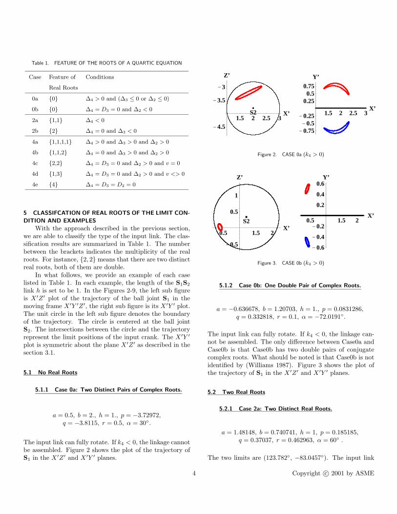
Table 1. FEATURE OF THE ROOTS OF A QUARTIC EQUATION

Case Feature of Conditions

Real Roots

0a {0} ∆4 > 0 and (∆3 ≤ 0 or ∆2 ≤ 0)

0b {0} ∆4 = D3 = 0 and ∆2 < 0

2a {1,1} ∆4 < 0

2b {2} ∆4 = 0 and ∆3 < 0

4a {1,1,1,1} ∆4 > 0 and ∆3 > 0 and ∆2 > 0

4b {1,1,2} ∆4 = 0 and ∆3 > 0 and ∆2 > 0

4c {2,2} ∆4 = D3 = 0 and ∆2 > 0 and v = 0

4d {1,3} ∆4 = D3 = 0 and ∆2 > 0 and v <> 0

4e {4} ∆4 = D3 = D2 = 0

5 CLASSIFCATION OF REAL ROOTS OF THE LIMIT CON-

DITION AND EXAMPLES

With the approach described in the previous section,we are able to classify the type of the input link. The clas-sification results are summarized in Table 1. The numberbetween the brackets indicates the multiplicity of the realroots. For instance, {2, 2} means that there are two distinctreal roots, both of them are double.

In what follows, we provide an example of each caselisted in Table 1. In each example, the length of the S1S2

link h is set to be 1. In the Figures 2-9, the left sub figureis X ′Z ′ plot of the trajectory of the ball joint S1 in themoving frame X ′Y ′Z ′, the right sub figure is its X ′Y ′ plot.The unit circle in the left sub figure denotes the boundaryof the trajectory. The circle is centered at the ball jointS2. The intersections between the circle and the trajectoryrepresent the limit positions of the input crank. The X ′Y ′

plot is symmetric about the plane X ′Z ′ as described in thesection 3.1.

5.1 No Real Roots

5.1.1 Case 0a: Two Distinct Pairs of Complex Roots.

a = 0.5, b = 2., h = 1., p = −3.72972,q = −3.8115, r = 0.5, α = 30◦.

The input link can fully rotate. If k4 < 0, the linkage cannotbe assembled. Figure 2 shows the plot of the trajectory ofS1 in the X ′Z ′ and X ′Y ′ planes.

1.5 2 2.5 3X’

-4.5

-3.5

-3

Z’

S2 1.5 2 2.5 3X’

-0.75-0.5-0.25

0.250.5

0.75

Y’

Figure 2. CASE 0a (k4 > 0)

0.5 1.5 2X’

-0.5

0.5

1

Z’

S2 0.5 1.5 2X’

-0.6

-0.4

-0.2

0.2

0.4

0.6Y’

Figure 3. CASE 0b (k4 > 0)

5.1.2 Case 0b: One Double Pair of Complex Roots.

a = −0.636678, b = 1.20703, h = 1., p = 0.0831286,q = 0.332818, r = 0.1, α = −72.0191◦.

The input link can fully rotate. If k4 < 0, the linkage can-not be assembled. The only difference between Case0a andCase0b is that Case0b has two double pairs of conjugatecomplex roots. What should be noted is that Case0b is notidentified by (Williams 1987). Figure 3 shows the plot ofthe trajectory of S1 in the X ′Z ′ and X ′Y ′ planes.

5.2 Two Real Roots

5.2.1 Case 2a: Two Distinct Real Roots.

a = 1.48148, b = 0.740741, h = 1, p = 0.185185,q = 0.37037, r = 0.462963, α = 60◦ .

The two limits are (123.782◦, −83.0457◦). The input link

4 Copyright c© 2001 by ASME

0.5 1 1.5X’

-0.5

0.5

1

Z’

S2 0.5 1 1.5X’

-1

-0.5

0.5

1Y’

Figure 4. CASE 2a

-0.5 0.5 1X’

-0.5

0.5

1

Z’

S2 -0.5 0.5 1X’

-0.4

-0.2

0.2

0.4Y’

Figure 5. CASE 2b (k4 > 0)

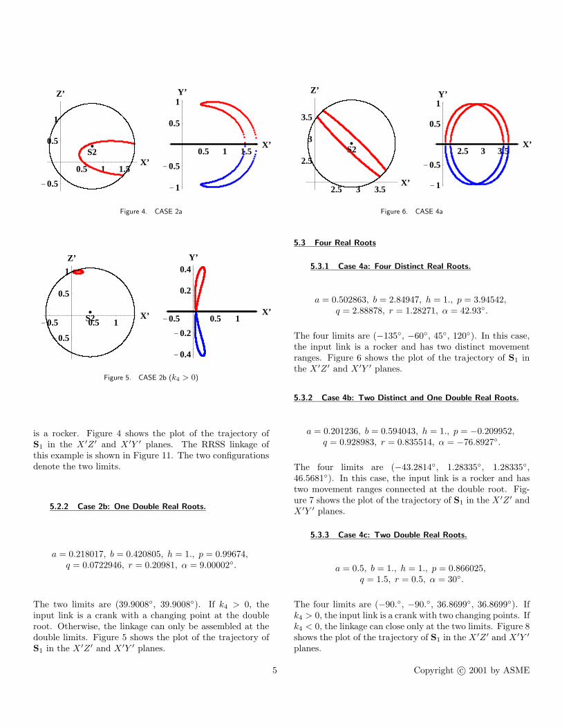
is a rocker. Figure 4 shows the plot of the trajectory ofS1 in the X ′Z ′ and X ′Y ′ planes. The RRSS linkage ofthis example is shown in Figure 11. The two configurationsdenote the two limits.

5.2.2 Case 2b: One Double Real Roots.

a = 0.218017, b = 0.420805, h = 1., p = 0.99674,q = 0.0722946, r = 0.20981, α = 9.00002◦.

The two limits are (39.9008◦, 39.9008◦). If k4 > 0, theinput link is a crank with a changing point at the doubleroot. Otherwise, the linkage can only be assembled at thedouble limits. Figure 5 shows the plot of the trajectory ofS1 in the X ′Z ′ and X ′Y ′ planes.

2.5 3 3.5X’

2.5

3

3.5

Z’

S2 2.5 3 3.5X’

-1

-0.5

0.5

1Y’

Figure 6. CASE 4a

5.3 Four Real Roots

5.3.1 Case 4a: Four Distinct Real Roots.

a = 0.502863, b = 2.84947, h = 1., p = 3.94542,q = 2.88878, r = 1.28271, α = 42.93◦.

The four limits are (−135◦, −60◦, 45◦, 120◦). In this case,the input link is a rocker and has two distinct movementranges. Figure 6 shows the plot of the trajectory of S1 inthe X ′Z ′ and X ′Y ′ planes.

5.3.2 Case 4b: Two Distinct and One Double Real Roots.

a = 0.201236, b = 0.594043, h = 1., p = −0.209952,q = 0.928983, r = 0.835514, α = −76.8927◦.

The four limits are (−43.2814◦, 1.28335◦, 1.28335◦,46.5681◦). In this case, the input link is a rocker and hastwo movement ranges connected at the double root. Fig-ure 7 shows the plot of the trajectory of S1 in the X ′Z ′ andX ′Y ′ planes.

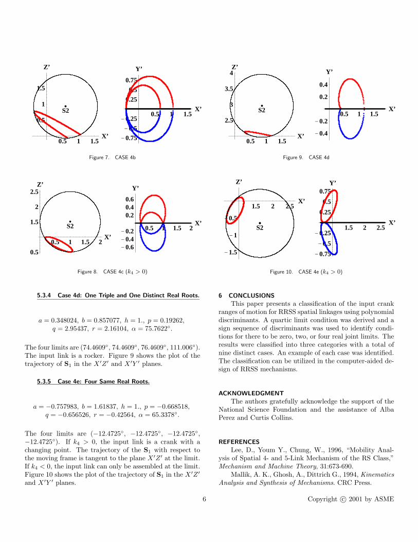
5.3.3 Case 4c: Two Double Real Roots.

a = 0.5, b = 1., h = 1., p = 0.866025,q = 1.5, r = 0.5, α = 30◦.

The four limits are (−90.◦, −90.◦, 36.8699◦, 36.8699◦). Ifk4 > 0, the input link is a crank with two changing points. Ifk4 < 0, the linkage can close only at the two limits. Figure 8shows the plot of the trajectory of S1 in the X ′Z ′ and X ′Y ′

planes.

5 Copyright c© 2001 by ASME

0.5 1 1.5X’

0.5

1

1.5

Z’

S2 0.5 1 1.5X’

-0.75

-0.5

-0.25

0.25

0.5

0.75

Y’

Figure 7. CASE 4b

0.5 1 1.5 2X’

0.5

1.5

2

2.5Z’

S2 0.5 1 1.5 2X’

-0.6-0.4-0.2

0.20.40.6

Y’

Figure 8. CASE 4c (k4 > 0)

5.3.4 Case 4d: One Triple and One Distinct Real Roots.

a = 0.348024, b = 0.857077, h = 1., p = 0.19262,q = 2.95437, r = 2.16104, α = 75.7622◦.

The four limits are (74.4609◦, 74.4609◦, 76.4609◦, 111.006◦).The input link is a rocker. Figure 9 shows the plot of thetrajectory of S1 in the X ′Z ′ and X ′Y ′ planes.

5.3.5 Case 4e: Four Same Real Roots.

a = −0.757983, b = 1.61837, h = 1., p = −0.668518,q = −0.656526, r = −0.42564, α = 65.3378◦.

The four limits are (−12.4725◦, −12.4725◦, −12.4725◦,−12.4725◦). If k4 > 0, the input link is a crank with achanging point. The trajectory of the S1 with respect tothe moving frame is tangent to the plane X ′Z ′ at the limit.If k4 < 0, the input link can only be assembled at the limit.Figure 10 shows the plot of the trajectory of S1 in the X ′Z ′

and X ′Y ′ planes.

0.5 1 1.5X’

2.5

3

3.5

4Z’

S2 0.5 1 1.5X’

-0.4

-0.2

0.2

0.4

Y’

Figure 9. CASE 4d

1.5 2 2.5X’

-1.5

-1

-0.5

Z’

S2 1.5 2 2.5X’

-0.75

-0.5

-0.25

0.25

0.5

0.75Y’

Figure 10. CASE 4e (k4 > 0)

6 CONCLUSIONS

This paper presents a classification of the input crankranges of motion for RRSS spatial linkages using polynomialdiscriminants. A quartic limit condition was derived and asign sequence of discriminants was used to identify condi-tions for there to be zero, two, or four real joint limits. Theresults were classified into three categories with a total ofnine distinct cases. An example of each case was identified.The classification can be utilized in the computer-aided de-sign of RRSS mechanisms.

ACKNOWLEDGMENT

The authors gratefully acknowledge the support of theNational Science Foundation and the assistance of AlbaPerez and Curtis Collins.

REFERENCES

Lee, D., Youm Y., Chung, W., 1996, “Mobility Anal-ysis of Spatial 4- and 5-Link Mechanism of the RS Class,”Mechanism and Machine Theory, 31:673-690.

Mallik, A. K., Ghosh, A., Dittrich G., 1994, KinematicsAnalysis and Synthesis of Mechanisms. CRC Press.

6 Copyright c© 2001 by ASME

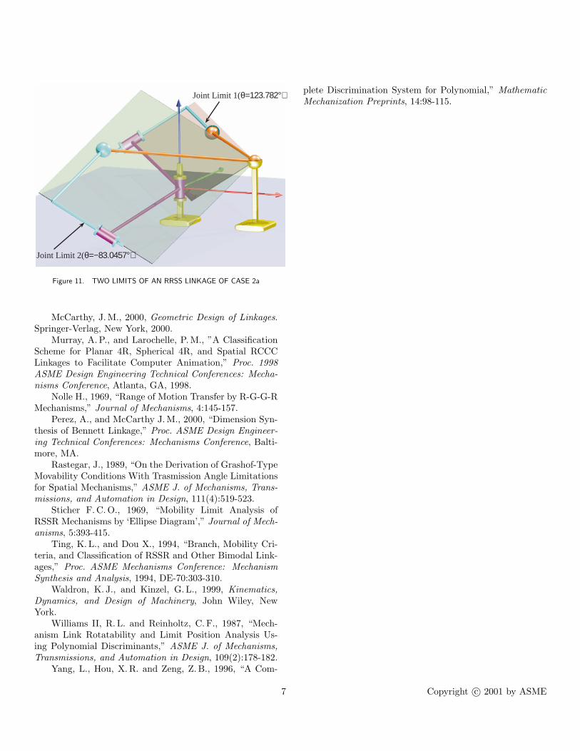
Joint Limit 2(θ=−83.0457°)

Joint Limit 1(θ=123.782°)

Figure 11. TWO LIMITS OF AN RRSS LINKAGE OF CASE 2a

McCarthy, J. M., 2000, Geometric Design of Linkages.Springer-Verlag, New York, 2000.

Murray, A. P., and Larochelle, P. M., ”A ClassificationScheme for Planar 4R, Spherical 4R, and Spatial RCCCLinkages to Facilitate Computer Animation,” Proc. 1998ASME Design Engineering Technical Conferences: Mecha-nisms Conference, Atlanta, GA, 1998.

Nolle H., 1969, “Range of Motion Transfer by R-G-G-RMechanisms,” Journal of Mechanisms, 4:145-157.

Perez, A., and McCarthy J. M., 2000, “Dimension Syn-thesis of Bennett Linkage,” Proc. ASME Design Engineer-ing Technical Conferences: Mechanisms Conference, Balti-more, MA.

Rastegar, J., 1989, “On the Derivation of Grashof-TypeMovability Conditions With Trasmission Angle Limitationsfor Spatial Mechanisms,” ASME J. of Mechanisms, Trans-missions, and Automation in Design, 111(4):519-523.

Sticher F. C. O., 1969, “Mobility Limit Analysis ofRSSR Mechanisms by ‘Ellipse Diagram’,” Journal of Mech-anisms, 5:393-415.

Ting, K. L., and Dou X., 1994, “Branch, Mobility Cri-teria, and Classification of RSSR and Other Bimodal Link-ages,” Proc. ASME Mechanisms Conference: MechanismSynthesis and Analysis, 1994, DE-70:303-310.

Waldron, K. J., and Kinzel, G. L., 1999, Kinematics,Dynamics, and Design of Machinery, John Wiley, NewYork.

Williams II, R. L. and Reinholtz, C. F., 1987, “Mech-anism Link Rotatability and Limit Position Analysis Us-ing Polynomial Discriminants,” ASME J. of Mechanisms,Transmissions, and Automation in Design, 109(2):178-182.

Yang, L., Hou, X. R. and Zeng, Z. B., 1996, “A Com-

plete Discrimination System for Polynomial,” MathematicMechanization Preprints, 14:98-115.

7 Copyright c© 2001 by ASME