bea.gov 1

Regional Price Parities

Bettina Aten, Eric Figueroa and Troy Martinrpp@bea.gov

Bureau of Economic Analysis

Pub

lic D

iscl

osur

e A

utho

rized

Pub

lic D

iscl

osur

e A

utho

rized

Pub

lic D

iscl

osur

e A

utho

rized

Pub

lic D

iscl

osur

e A

utho

rized

bea.gov 2

OverviewSpatial vs Time-to-time Price Indexes

1. Multilateral Price indexes:

▪ PPPs (purchasing power parities) in the international literature, with

a choice of numeraire currency, such as Euro, or US Dollar

▪ RPPs (regional price parities) within a country, same currency

2. Other types of Spatial Price indexes:

� Bilateral

� Cost of Living

bea.gov 3

Overview of BEA-BLS-Census Collaboration

� Office of Prices and Living Conditions at the Bureau of Labor

Statistics (BLS)

� CPI prices

� Expenditure weights

� Poverty Statistics Branch, Housing and Household Economic

Statistics (HHES) at the Census Bureau

� American Community Survey

� Housing survey

bea.gov 4

Overview of Data

1. Consumer Price Index (CPI) micro data on prices from BLS

� 207 item strata, 38 urban areas (1 million observations / year)

� Rents and Owners’ Equivalent Rents (34,000 observations / year)

2. Consumer Expenditure Survey (CE) weights data from BLS

� 207 item-level weights x 38 urban areas

� Plus 207 item-level weights x 4 rural areas

3. American Community Survey (ACS) from Census

� 51 states, 363 metro areas, 3143 counties: Rent price levels

� 5 year rolling average for all counties (10 million observations for 5 years)

bea.gov 5

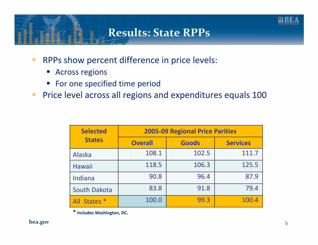
Results: State RPPs

� RPPs show percent difference in price levels:

� Across regions

� For one specified time period

� Price level across all regions and expenditures equals 100

Selected

States

2005-09 Regional Price Parities

Overall Goods Services

Alaska 108.1 102.5 111.7

Hawaii 118.5 106.3 125.5

Indiana 90.8 96.4 87.9

South Dakota 83.8 91.8 79.4

All States * 100.0 99.3 100.4

* Includes Washington, DC.

bea.gov 6

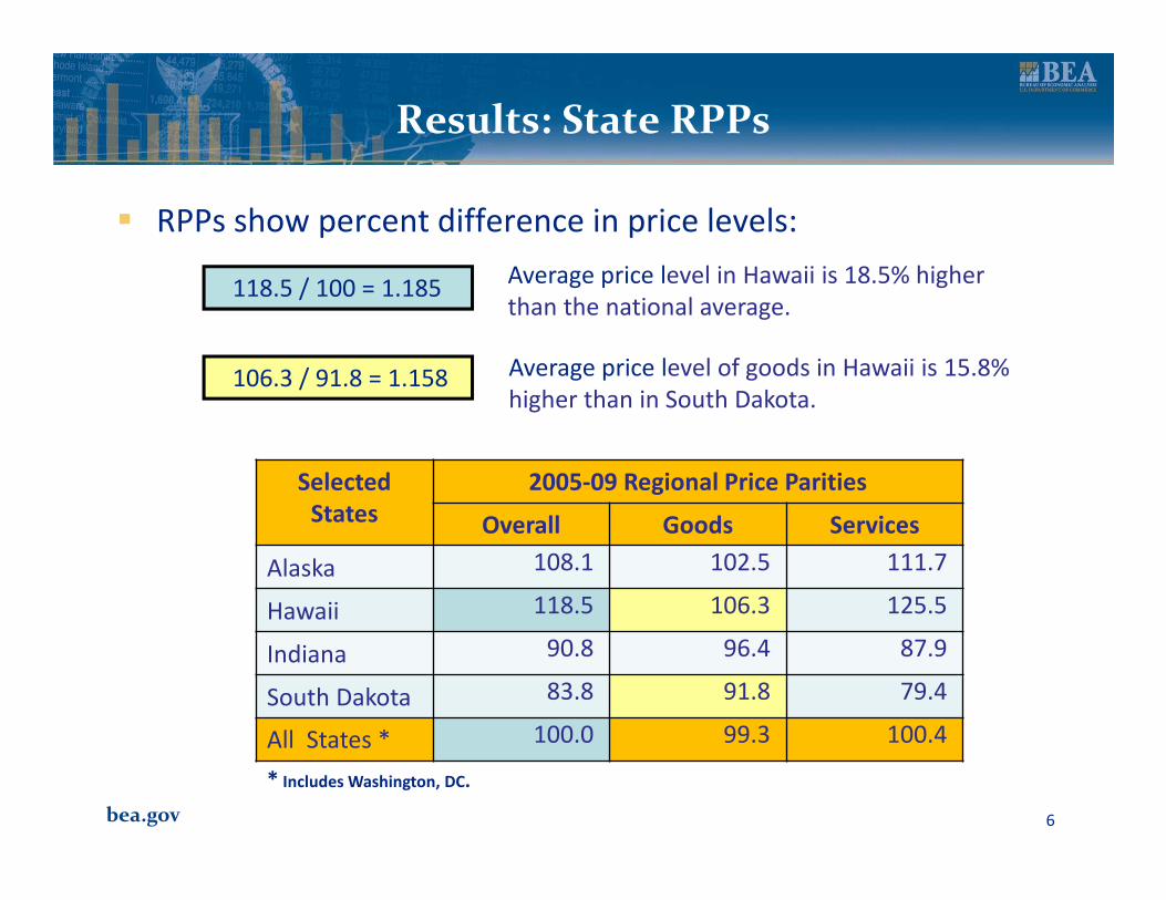
Results: State RPPs

� RPPs show percent difference in price levels:

Selected

States

2005-09 Regional Price Parities

Overall Goods Services

Alaska 108.1 102.5 111.7

Hawaii 118.5 106.3 125.5

Indiana 90.8 96.4 87.9

South Dakota 83.8 91.8 79.4

All States * 100.0 99.3 100.4

118.5 / 100 = 1.185

* Includes Washington, DC.

106.3 / 91.8 = 1.158

Average price level in Hawaii is 18.5% higher

than the national average.

Average price level of goods in Hawaii is 15.8%

higher than in South Dakota.

bea.gov 7

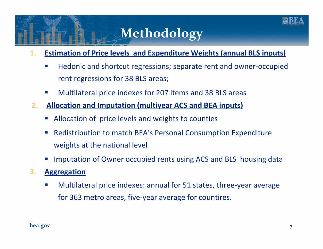
Methodology

1. Estimation of Price levels and Expenditure Weights (annual BLS inputs)

� Hedonic and shortcut regressions; separate rent and owner-occupied

rent regressions for 38 BLS areas;

� Multilateral price indexes for 207 items and 38 BLS areas

2. Allocation and Imputation (multiyear ACS and BEA inputs)

� Allocation of price levels and weights to counties

� Redistribution to match BEA’s Personal Consumption Expenditure

weights at the national level

� Imputation of Owner occupied rents using ACS and BLS housing data

3. Aggregation

� Multilateral price indexes: annual for 51 states, three-year average

for 363 metro areas, five-year average for countires.

bea.gov 8

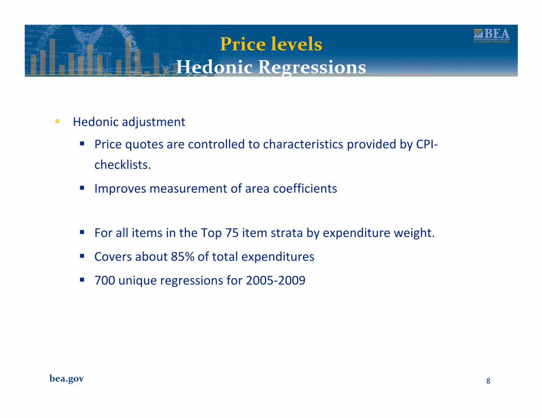
Price levelsHedonic Regressions

� Hedonic adjustment

� Price quotes are controlled to characteristics provided by CPI-

checklists.

� Improves measurement of area coefficients

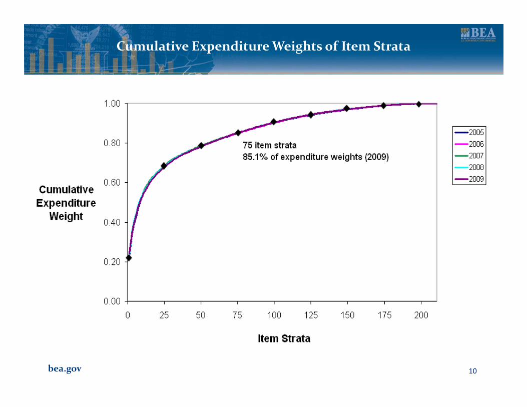
� For all items in the Top 75 item strata by expenditure weight.

� Covers about 85% of total expenditures

� 700 unique regressions for 2005-2009

bea.gov 9

Multilateral Aggregation (3) Weighted CPD

3. WCPD (Weighted CPD)

ln , weighted by

ln

c c c c

n n n n

c c

WCPD

p s

P

α β ε

α

= + +

=

The Weighted CPD index is a weighted average of the logarithms of the price relatives with weights that are harmonic means of the budget shares in the two areas.

Notation and formulas follow Deaton & Dupriez (2009).

P = price index, p = item price, s = budget share, q = notional quantity

Subscript i = 1…N indicates items; j = 1…M indicates areas; c, d indicate areas c,d.

bea.gov 10

Cumulative Expenditure Weights of Item Strata

bea.gov 11

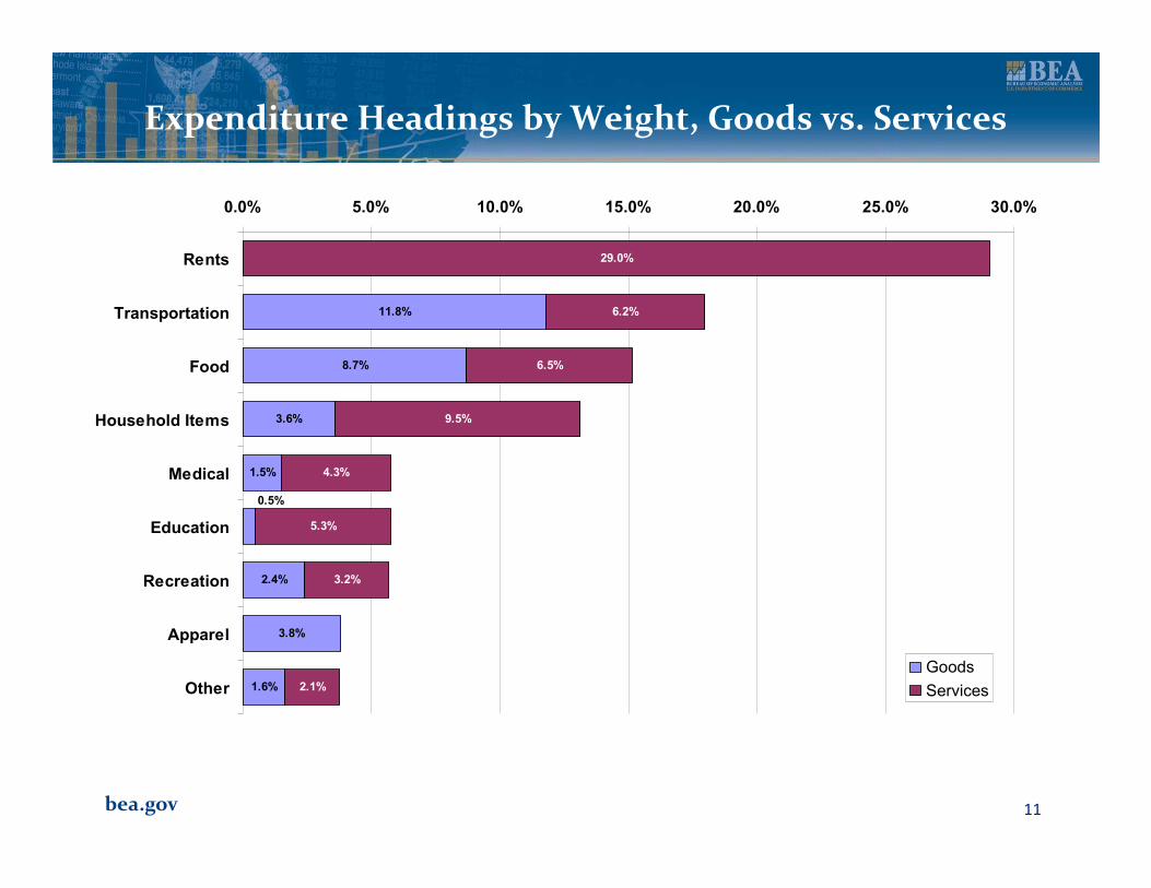
Expenditure Headings by Weight, Goods vs. Services

11.8%

8.7%

3.6%

1.5%

2.4%

3.8%

1.6%

29.0%

6.2%

6.5%

9.5%

4.3%

5.3%

3.2%

2.1%

0.5%

0.0% 5.0% 10.0% 15.0% 20.0% 25.0% 30.0%

Rents

Transportation

Food

Household Items

Medical

Education

Recreation

Apparel

Other

Goods

Services

bea.gov 12

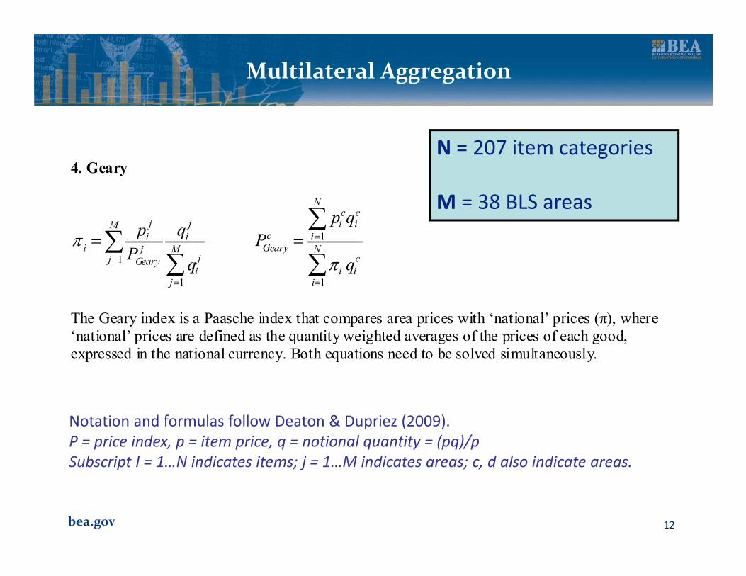
Multilateral Aggregation

Notation and formulas follow Deaton & Dupriez (2009).

P = price index, p = item price, q = notional quantity = (pq)/p

Subscript I = 1…N indicates items; j = 1…M indicates areas; c, d also indicate areas.

4. Geary

1

1

1 1

c c

j j i iMci i i

i GearyM jj cj Gearyi i i

j i

p qp q

PP

q q

ππ

=

=

= =

= =∑

∑∑ ∑

The Geary index is a Paasche index that compares area prices with ‘national’ prices (π), where ‘national’ prices are defined as the quantity weighted averages of the prices of each good, expressed in the national currency. Both equations need to be solved simultaneously.

N = 207 item categories

M = 38 BLS areas

bea.gov 13

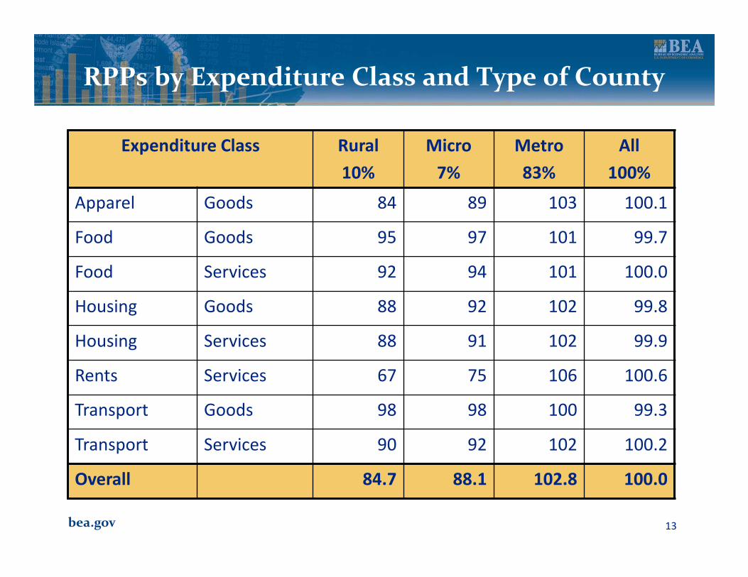
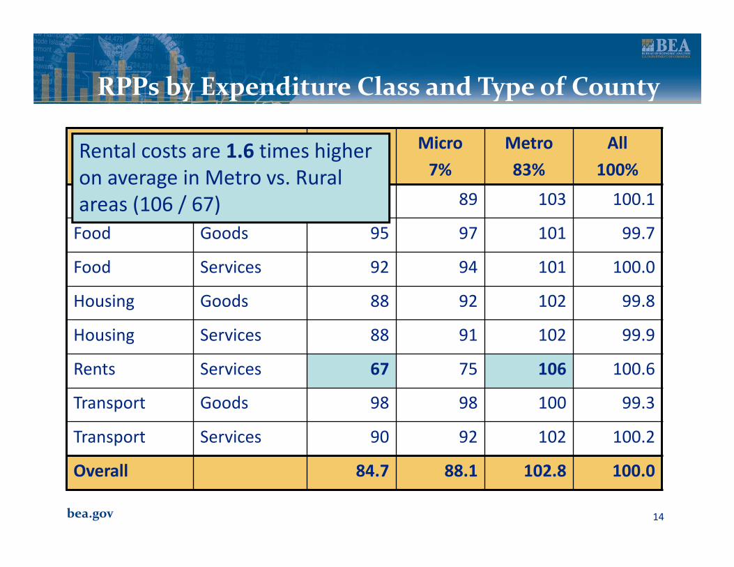
RPPs by Expenditure Class and Type of County

Expenditure Class Rural

10%

Micro

7%

Metro

83%

All

100%

Apparel Goods 84 89 103 100.1

Food Goods 95 97 101 99.7

Food Services 92 94 101 100.0

Housing Goods 88 92 102 99.8

Housing Services 88 91 102 99.9

Rents Services 67 75 106 100.6

Transport Goods 98 98 100 99.3

Transport Services 90 92 102 100.2

Overall 84.7 88.1 102.8 100.0

bea.gov 14

Expenditure Class Rural

10%

Micro

7%

Metro

83%

All

100%

Apparel Goods 84 89 103 100.1

Food Goods 95 97 101 99.7

Food Services 92 94 101 100.0

Housing Goods 88 92 102 99.8

Housing Services 88 91 102 99.9

Rents Services 67 75 106 100.6

Transport Goods 98 98 100 99.3

Transport Services 90 92 102 100.2

Overall 84.7 88.1 102.8 100.0

Rental costs are 1.6 times higher

on average in Metro vs. Rural

areas (106 / 67)

RPPs by Expenditure Class and Type of County

bea.gov 15

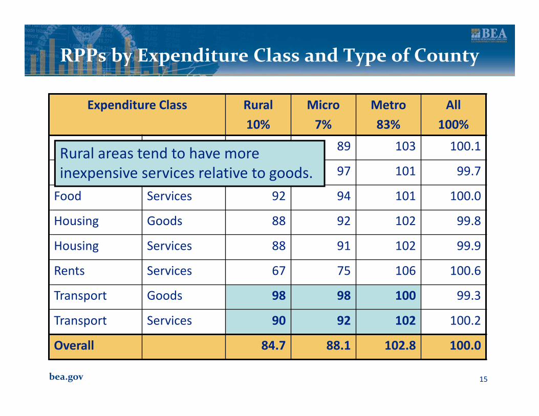
Expenditure Class Rural

10%

Micro

7%

Metro

83%

All

100%

Apparel Goods 84 89 103 100.1

Food Goods 95 97 101 99.7

Food Services 92 94 101 100.0

Housing Goods 88 92 102 99.8

Housing Services 88 91 102 99.9

Rents Services 67 75 106 100.6

Transport Goods 98 98 100 99.3

Transport Services 90 92 102 100.2

Overall 84.7 88.1 102.8 100.0

Rural areas tend to have more

inexpensive services relative to goods.

RPPs by Expenditure Class and Type of County

bea.gov 16

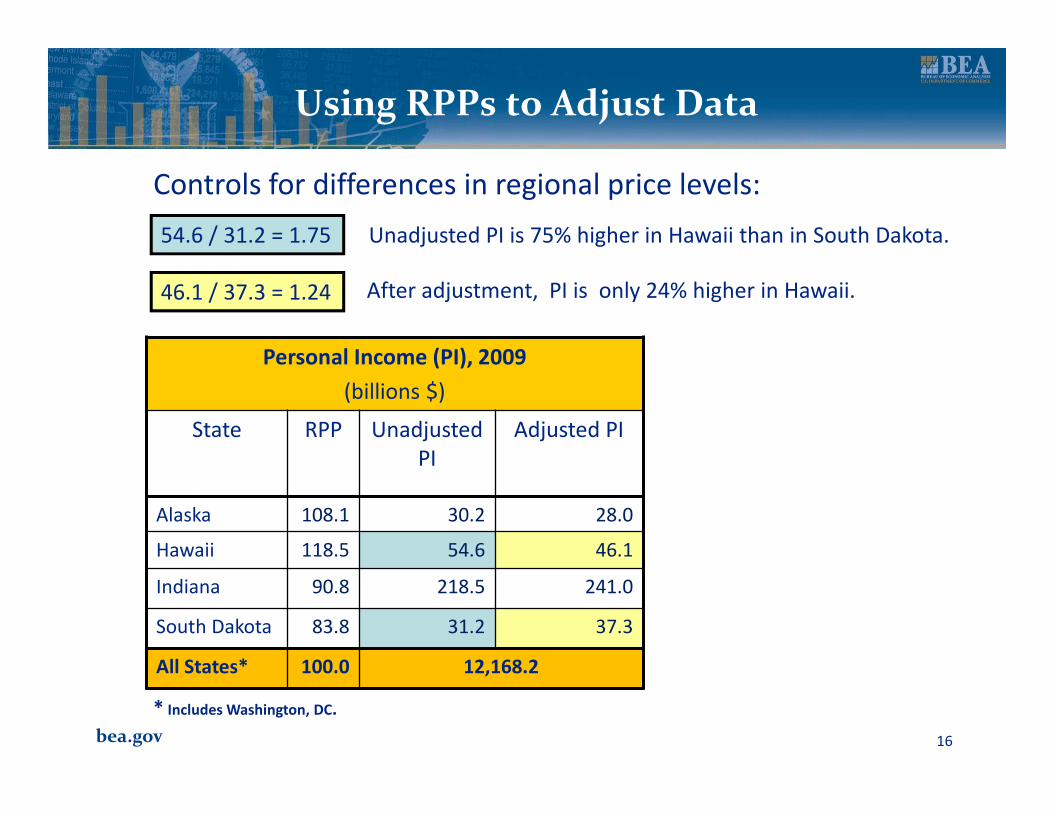
46.1 / 37.3 = 1.24

Using RPPs to Adjust Data

Controls for differences in regional price levels:

Personal Income (PI), 2009

(billions $)

State RPP Unadjusted

PI

Adjusted PI

Alaska 108.1 30.2 28.0

Hawaii 118.5 54.6 46.1

Indiana 90.8 218.5 241.0

South Dakota 83.8 31.2 37.3

All States* 100.0 12,168.2

* Includes Washington, DC.

54.6 / 31.2 = 1.75 Unadjusted PI is 75% higher in Hawaii than in South Dakota.

After adjustment, PI is only 24% higher in Hawaii.

bea.gov 17

bea.gov 18

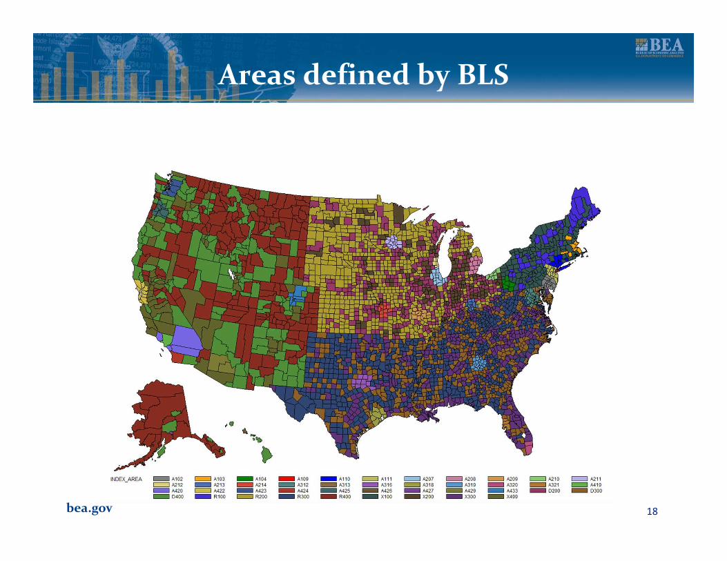
Areas defined by BLS

bea.gov 19

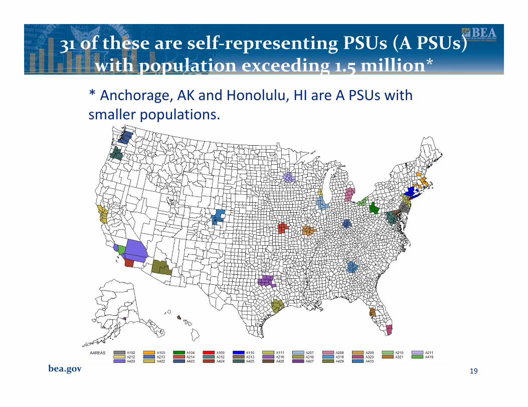
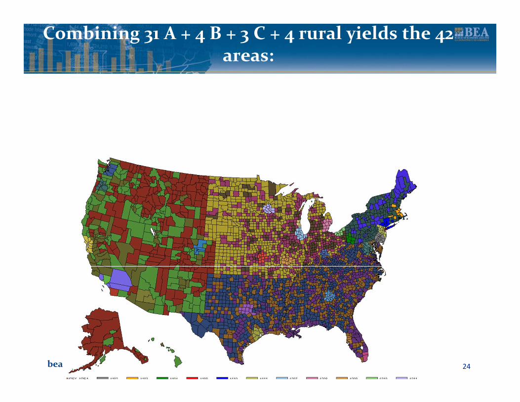
31 of these are self-representing PSUs (A PSUs) with population exceeding 1.5 million*

* Anchorage, AK and Honolulu, HI are A PSUs with

smaller populations.

bea.gov 20

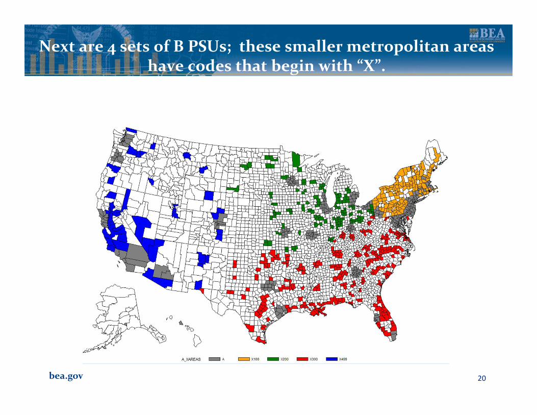
Next are 4 sets of B PSUs; these smaller metropolitan areas have codes that begin with “X”.

bea.gov 21

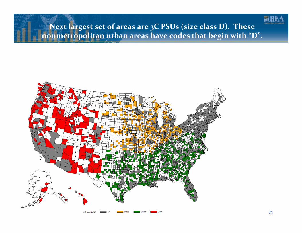
Next largest set of areas are 3C PSUs (size class D). These nonmetropolitan urban areas have codes that begin with “D”.

bea.gov 22

Together, the A, B and C PSU’s make up the urban portion of the US.

bea.gov 23

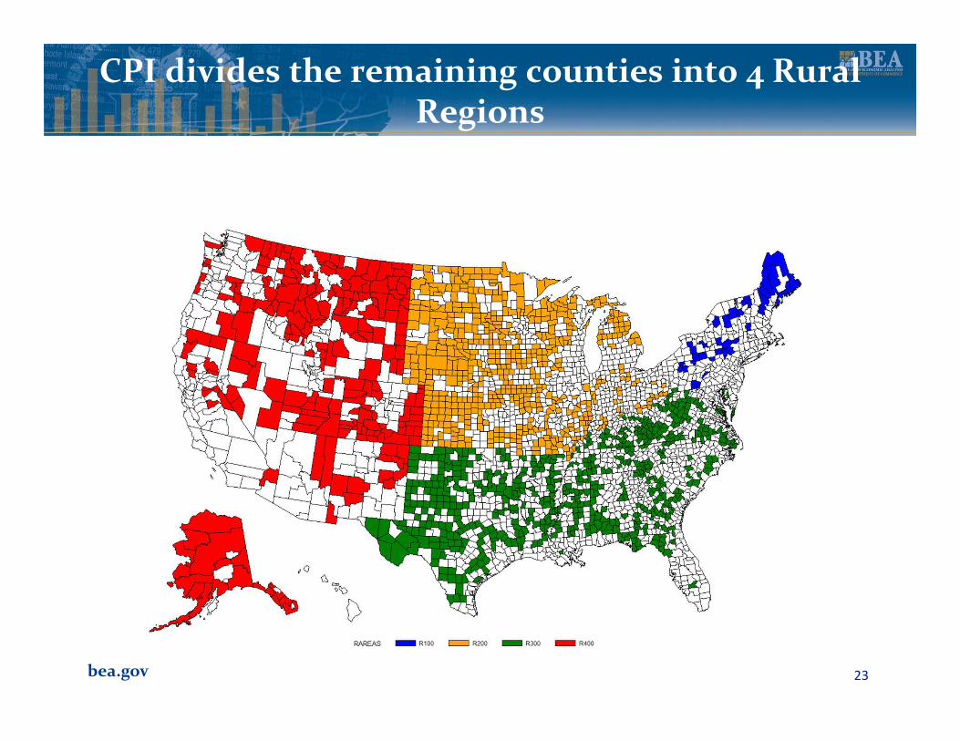
CPI divides the remaining counties into 4 Rural Regions

bea.gov 24

Combining 31 A + 4 B + 3 C + 4 rural yields the 42 areas:

bea.gov 25

Allocations

� Assumptions:

1. Price levels of the counties within BLS areas equal the price level of the

BLS area

2. Expenditure weights within areas proportional to income

� Except for Rents:

� Use actual ACS county level observations on Rent price levels and expenditures

� Use BLS relationship between Rent price level and Owner-occupied price levels to

impute Owner-occupied rent expenditures, by type of structure and number of

bedrooms

bea.gov 26

ACS Rents

� Close collaboration with the Poverty Statistics Branch of the Housing and

Household Economic Statistics Division (HHES) of the Census Bureau to

process the housing component of the ACS

� American Community Survey ( multiyear rolling average for all counties in

the U.S.)

� About 3 million observations on rents in the housing survey

� Hedonic regression for individual housing units

� Dependent variable = log of gross rents ($)

� Characteristics include number of bedrooms, type of unit (apartment, detached

house, etc.), year built, total number of rooms, and the survey year (2005-2009)

� Geographic coefficients by state (51 including DC), metro areas (366 as defined by

OMB) and three groupings (metro, micro and rural) also OMB defined

bea.gov 27

Final Multilateral Aggregation

1. Five-year averages for BLS price levels� Food, Apparel, Education, Medical, Transport, Recreation, Housing

(excluding Rents) and Other goods

2. Multiyear Rent and Owner-occupied rent levels:

1. Annual for States

2. Three-year for MSAs

3. Five-year for counties

� One RPP for each state, metro area and type of county

bea.gov 28

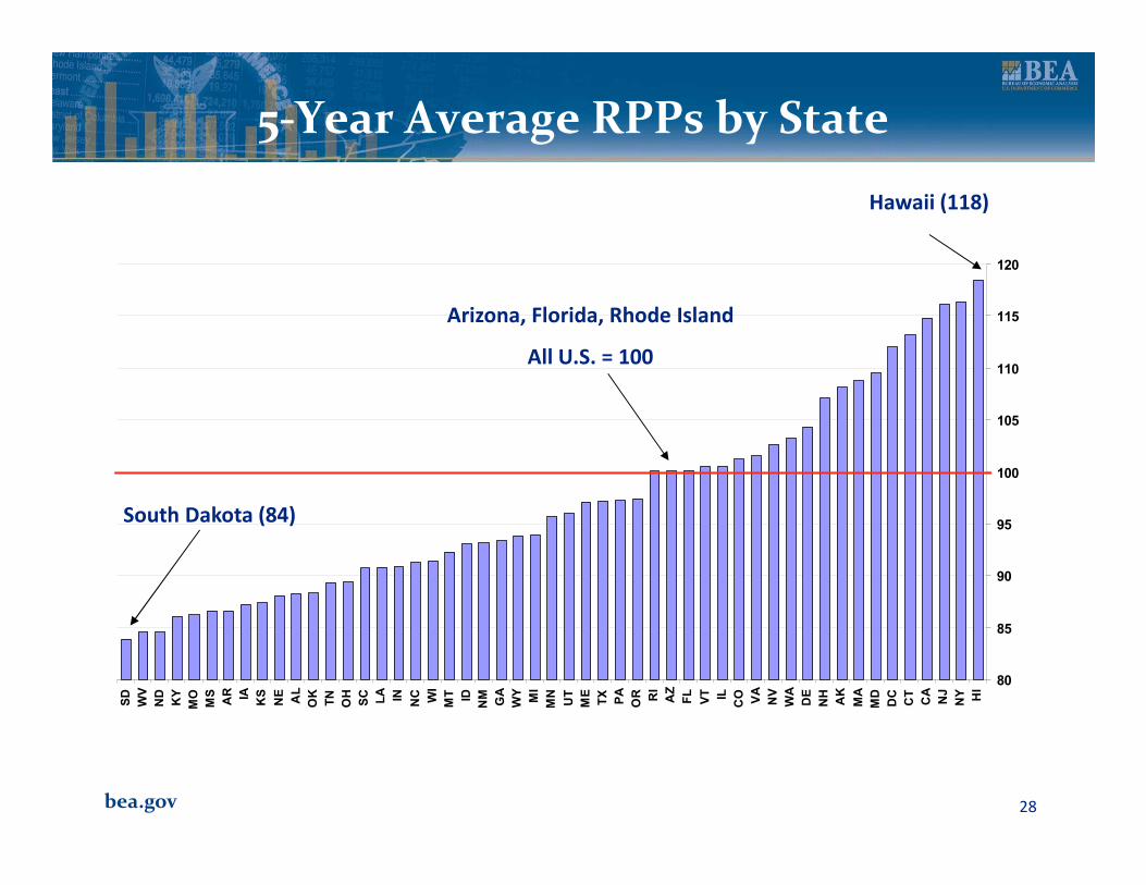
5-Year Average RPPs by State

80

85

90

95

100

105

110

115

120

HI

NY

NJ

CA

CT

DC

MD

MA

AK

NH

DE

WA

NV

VA

COILVT

FL

AZ

RI

OR

PA

TX

ME

UT

MNMI

WY

GA

NMID

MT

WI

NCINLA

SC

OH

TN

OK

AL

NE

KSIA

AR

MS

MO

KY

ND

WV

SD

South Dakota (84)

Hawaii (118)

Arizona, Florida, Rhode Island

All U.S. = 100

bea.gov 29

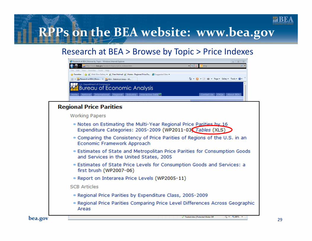
RPPs on the BEA website: www.bea.gov

Research at BEA > Browse by Topic > Price Indexes

bea.gov 30

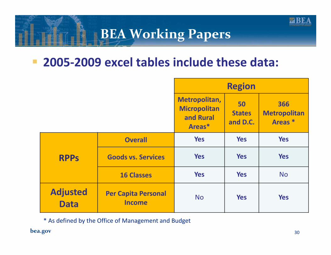
� 2005-2009 excel tables include these data:

BEA Working Papers

Region

Metropolitan,

Micropolitan

and Rural

Areas*

50

States

and D.C.

366

Metropolitan

Areas *

RPPs

Overall Yes Yes Yes

Goods vs. Services Yes Yes Yes

16 Classes Yes Yes No

Adjusted

DataPer Capita Personal

IncomeNo Yes Yes

* As defined by the Office of Management and Budget

bea.gov 31

Future Development

� RPPs by States, Metro and County Type for 2006-2010

� May 2012

� RPPs using Personal Consumption Expenditures (BEA concept)

� Currently using Consumption Expenditure concept used at BLS

� Differences in weights and coverage

� Owner-Occupied Rent price levels and expenditures

� Currently using Rents for both Renters and Owner-Occupied homes

bea.gov 32

Selected References

� ACS estimates of geographic differences can be found at: http://www.census.gov/hhes/povmeas/publications/working.html

� Deaton, Angus. “Price Indexes, Inequality, and the Measurement of World Poverty.” American Economic Review 2010, 100:1, 5-34.

� Deaton, Angus and Olivier Dupriez. “Purchasing Power Parity Exchange Rates for the Global Poor.” http://princeton.edu/~deaton/downloads/Purchasing_power_parity_exchange_rates_for_global_poor_Nov11.pdf

� Renwick, Trudi. “Alternative Geographic Adjustments of U.S. Poverty Thresholds: Impact on State Povery Rates.” U.S. Census Bureau 2009, http://www.census.gov/hhes/www/povmeas/papers/Geo-Adj-Pov-Thld8.pdf

� Verbrugge, Randal and Thesia Garner. “Reconciling User Costs and Rental Equivalence: Evidence from the U.S. Consumer Expenditure Survey.” U.S. Bureau of Labor Statistics 2009, Working Papers 247.

bea.gov 33

Multilateral Aggregation (1) Gini-EKS Tornqvist

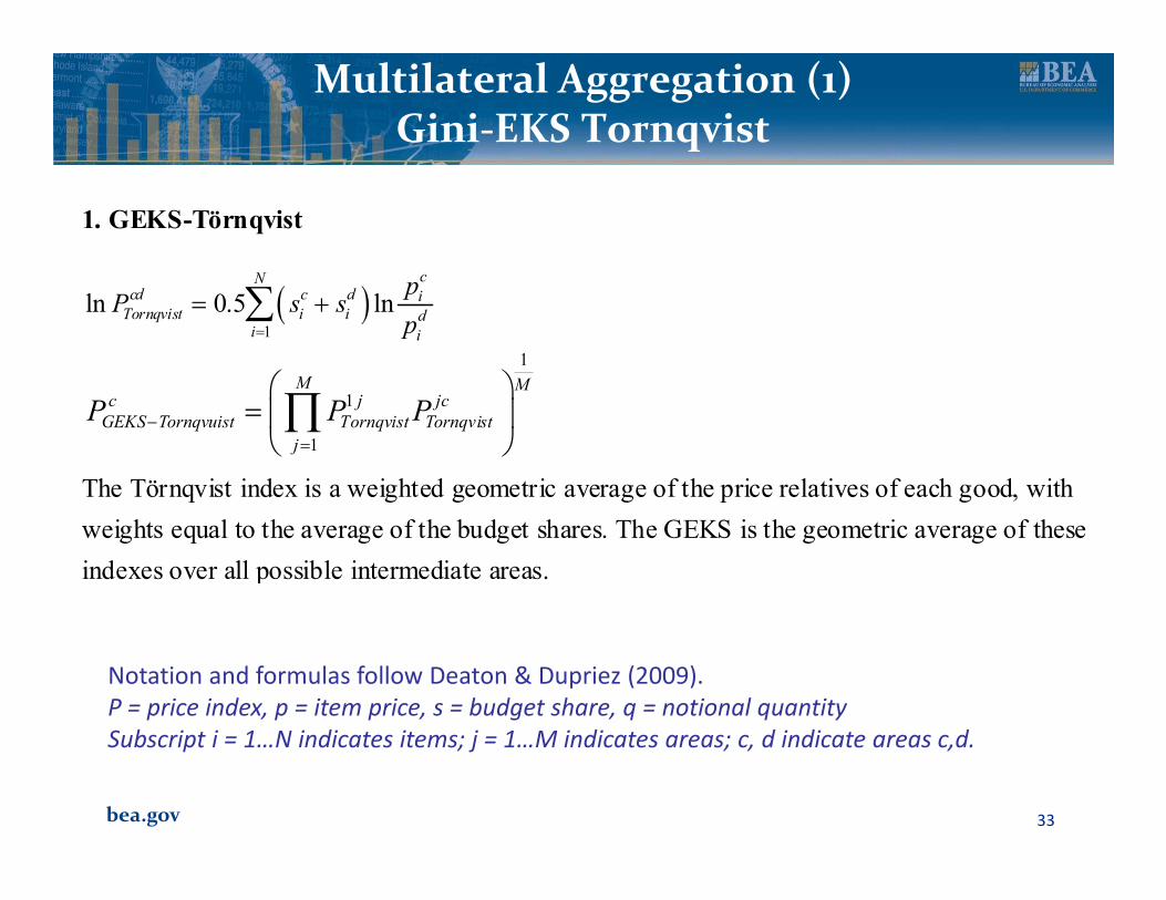
1. GEKS-Törnqvist

( )1

ln 0.5 ln

ccd c d iTornqvist i i d

i i

pP s s

p=

= +∑

1

1

1

M Mc j jc

GEKS Tornqvuist Tornqvist Tornqvist

j

P P P−=

= ∏

The Törnqvist index is a weighted geometric average of the price relatives of each good, with

weights equal to the average of the budget shares. The GEKS is the geometric average of these

indexes over all possible intermediate areas.

Notation and formulas follow Deaton & Dupriez (2009).

P = price index, p = item price, s = budget share, q = notional quantity

Subscript i = 1…N indicates items; j = 1…M indicates areas; c, d indicate areas c,d.

bea.gov 34

Multilateral Aggregation (2) Gini-EKS Fisher

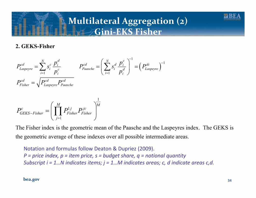
Notation and formulas follow Deaton & Dupriez (2009).

P = price index, p = item price, s = budget share, q = notional quantity

Subscript i = 1…N indicates items; j = 1…M indicates areas; c, d indicate areas c,d.

2. GEKS-Fisher

( )1

1

1 1

d c cd c cd d dci iLaspeyre i Paasche i Laspeyrec d

i ii i

p pP s P s P

p p

−−

= =

= = =

∑ ∑

cd cd cd

Fisher Laspeyre PaascheP P P=

1

1

1

M Mc j jc

GEKS Fisher Fisher Fisher

j

P P P−=

= ∏

The Fisher index is the geometric mean of the Paasche and the Laspeyres index. The GEKS is

the geometric average of these indexes over all possible intermediate areas.