KUNGL TEKNISKA HÖGSKOLANInstitutionen förSignaler, Sensorer & SystemSignalbehandling100 44 STOCKHOLM

ROYAL INSTITUTEOF TECHNOLOGY

Department ofSignals, Sensors & Systems

Signal ProcessingS-100 44 STOCKHOLM

Exact and Large Sample ML Techniques for

Parameter Estimation and Detection in Array

Processing

B� Ottersten� M� Viberg� P� Stoica� A� Nehorai

February ��� ����

TRITA�SB����

Chapter �

Exact and Large Sample ML

Techniques for Parameter

Estimation and Detection in Array

Processing

B� Ottersten�

M� Viberg�

P� Stoica�

A� Nehorai�

To appear in �Radar Array Processing��

Simon Haykin �ed��� Springer�Verlag�

�Bj�orn Ottersten and Mats Viberg are with the Department of Electrical Engineering� Link�opingUniversity� S���� �� Link�oping� Sweden

�Petre Stoica is with the Department of Control and Computers� Polytechnic Institute of Bucharest�Splaiul Independentei ���� R� �� Bucharest� Romania and his work was partially supported bygrants from the Swedish Intitute and the Royal Swedish Academy of Engineering Sciences�

�Arye Nehorai is with the Department of Electrical Engineering� Yale University� P�O� Box ��� YaleStation� New Haven� CT ���� USA and his work was supported by the AFOSR under Grant No�AFOSR � ��� and by the O�ce of Naval Research�

��� Introduction

Sensor array signal processing deals with the problem of extracting information from

a collection of measurements obtained from sensors distributed in space� The number

of signals present is assumed to be nite� and each signal is parametrized by a nite

number of parameters� Based on measurements of the array output� the objective is to

estimate the signals and their parameters� This research area has attracted considerable

interest for several years� A vast number of algorithms has appeared in the literature for

estimating unknown signal parameters from the measured output of a sensor array�

The interest in sensor array processing stems from the many applications where emit�

ter waveforms are measured at several points in space and�or time� In radar applications�

as discussed in Chapters � and � the objective is to determine certain parameters asso�

ciated with each return signal� these may include bearing� elevation� doppler shift� etc�

By using an array of antenna receivers� the accuracy with which the signal parameters

can be determined is greatly improved as compared to single�receiver systems�

As the signal environment becomes more dense� both in space and frequency� sensor

arrays will play a more signicant role in the eld of radio and microwave commu�

nications� Communication satellites placed in geostationary orbits are faced with an

increasing amount of channel interference because of limited space and a limited fre�

quency band� By utilizing the spatial selectivity that may be obtained with an array

of sensors� satellites operating in the same frequency band can be placed close together

without unacceptable interference� Mobile communication systems are faced with the

same problem� An increasing demand for mobile telephones and a limited bandwidth

has increased the number of base stations serving an area� If a base station is equipped

with a collection of receiving antennas� the spatial dimension can be used to distinguish

emitters� By appropriately processing the output of the antenna array� undesirable noise

and interference can be suppressed in favor of the signal�of�interest�

Underwater arrays with acoustical sensors �hydrophones� are frequently used in

surveillance� Several hydrophones are either towed behind a vessel or dropped in the

ocean to passively measure acoustical energy from other vessels� The objective is to de�

tect and estimate incoming signals in order to locate and identify vessels� In geophysical

�

exploration the ground is often excited by a detonation and waves re�ected from bound�

aries between layers in the earth are sensed by an array of geophones� By identifying the

wavefronts arriving at the array� information about the structure of the earth is inferred�

A common feature in the applications mentioned above is that several superimposed

waveelds are sampled both in space and in time� The same basic data model is there�

fore useful in all of these problems� Each application does� however� have aspects that

either complicate or simplify the estimation and detection procedures� In an underwater

environment� the propagation medium is often quite inhomogeneous and the wavefront

is dispersed and degraded� On the other hand� electromagnetic propagation in the atmo�

sphere is often well modeled as homogeneous propagation� An important complication

in� for example� radar systems arises from multipath propagation� i�e�� scenarios in which

scaled and delayed versions of the same wavefront impinge on the array from di�erent

directions�

It should also be noted that there are strong connections between array signal pro�

cessing and the harmonic retrieval problem� statistical factor analysis� and identication

of linear systems as well�

���� Background

Classical beamforming techniques were the rst attempts to utilize an array of sensors

to increase antenna aperture and directivity� By forming a weighted sum of the sensor

outputs� signals from certain directions are coherently added while incoherently adding

the noise and signals from other directions� The antenna is steered to di�erent directions

by altering the sensor weights� Adaptive antennas were later developed� in which the

sensor weights are updated on�line attempting to maximize desired signal energy while

suppressing interference and noise� Beamforming and adaptive antenna techniques have

been extensively studied in many books and papers� see for example ������� Details of

implementation are found in Chapter � of this book� whereas Chapter � is devoted to

beamforming in two dimensions �e�g�� azimuth and elevation�� Chapter � presents an

application to an imaging system� In the presence of multiple closely spaced sources�

beamforming techniques cannot provide consistent parameter estimates� The accuracy of

the estimates is not constrained by the amount of data� but rather by the array geometry

and sensor responses� which limit the resolution capabilities of these methods�

The availability of accurate and inexpensive analog to digital converters allows the de�

sign of arrays where each sensor output is digitized individually� This greatly expands the

signal processing possibilities for the array data� Identication methods adopted from

time series analysis were applied to the sensor array processing problem and demon�

strated a performance advantage relative to beamforming techniques� �������

The introduction of the MUSIC �MUltiple SIgnal Classication� algorithm �������

�see also ����� a generalization of Pisarenko�s harmonic retrieval method ���� provided

a new geometric interpretation for the sensor array processing problem� This was an

attempt to more fully exploit the correct underlying model of the parametrized sensor

array problem� The MUSIC data model is formulated using concepts of complex vector

spaces� and powerful matrix algebra tools are applied to the problem� Currently� the vec�

tor space formulation of the sensor array problem is used extensively� This has resulted

in a large number of algorithms� often referred to as eigenvector or subspace techniques�

see e�g� ���������

The MUSIC algorithm is based on a known parametrization of the array response�

which leads to a parametrized model of the sensor array output� When cast in an

appropriate statistical framework� the Maximum Likelihood �ML� parameter estimate

can be derived for the sensor array problem� ML estimation is a systematic approach to

many parameter estimation problems� and ML techniques for the sensor array problem

have been studied by a number of researchers� see for example ��������� Within the

vector space formulation� di�erent probabilistic models have been used for the emitter

signals� Performance bounds �Cram�er�Rao bounds� on the estimation error covariance

can be derived based on the di�erent model assumptions� see ��� and ������ ���

Unfortunately� the ML estimation method generally requires a multidimensional non�

linear optimization at a considerable computational cost� Reduced computational com�

plexity is usually achieved by use of a suboptimal estimator� in which case the quality

of the estimate is an issue� Determining what is an accurate estimator is in general a

very di�cult task� However� an analysis is possible� for example� when assuming a large

amount of data� Although asymptotic in character� these results are often useful for

�

algorithm comparison as well as for predicting estimation accuracy in realistic scenarios�

Therefore� there has recently been a great interest in analytic performance studies of

array processing algorithms� The MUSIC algorithm� because of its generality and pop�

ularity� has received the most attention� see e�g� ���� �� � and � ��� ��� Analysis of

other subspace based algorithms is found in� for example ���� �� and � ��������

���� Chapter Outline

This chapter attempts to establish a connection between the classical ML estimation

techniques and the more recent eigenstructure or subspace based methods� The estima�

tors are related in terms of their asymptotic behavior and also compared to performance

bounds� Computational schemes for calculating the estimates are also presented�

An optimal subspace based technique termed WSF �weighted subspace tting� is

discussed in some more detail� The detection problem is also addressed and a hypothesis

testing scheme� based on the WSF criterion� is presented� The estimation and detection

methods discussed herein are applicable to arbitrary array congurations and emitter

signals� The case of highly correlated or even coherent sources �specular multipath��

which is particularly relevant in radar applications� is given special attention�

The chapter is organized as follows� Section ��� presents a data model and the

underlying assumptions� In Section �� � two probabilistic models are formulated as well

as the corresponding ML estimators� Multidimensional subspace based methods� their

asymptotic properties� and the relation to the ML estimators is the topic of Section ����

In Section ���� a Newton type algorithm is applied to the various cost functions and

its computational complexity is discussed� Section ��� presents schemes for detecting

the number of signals� The performance of the estimation and detection procedures is

examined through numerical examples and simulations in Section ����

�

��� Sensor Array Processing

This section presents the mathematical model of the array output and introduces the

basic assumptions� Consider the scenario of Figure ��� An array of m sensors arranged

Figure ���� A passive sensor array receiving emitter signals from point sources�

in an arbitrary geometry� receives the waveforms generated by d point sources� The

output of each sensor is modeled as the response of a linear time�invariant system� Let

hki�t� be the impulse response of the kth sensor to a signal �si�t� impinging on the array�

The impulse response depends on the physical antenna structure� the receiver electronics�

other antennas in the array through mutual coupling� as well as the signal parameters�

The time delay of the ith signal at the kth array element� relative to some xed reference

point� is denoted �ki� The output of the kth array element can then be written as a

superposition

�xk�t� dXi��

hki�t� � �si�t� �ki� ! �nk�t� � ����

where ��� denotes convolution and �nk�t� is an additive noise term independent of �si�t��The sensor outputs are collected in the m�vector

�x�t�

��������x��t����

�xm�t�

������� �������Pd

i�� h�i � �si�t� ��i

���Pd

i�� hmi � �si�t� �mi

�������!��������n��t����

�nm�t�

������� � �����

�

���� Narrowband Data Model

Consider an emitter signal �s�t� and express this signal in terms of a center frequency �

�s�t� ��t� cos��t! ��t�� � ��� �

If the amplitude� ��t�� and phase� ��t�� of the signal vary slowly relative to the propa�

gation time across the array � � i�e�� if

��t� � � � ��t� ��t� � � � ��t� � �����

the signal is said to be narrowband� The narrowband assumption implies that

�s�t� � � ��t� � � cos���t� � � ! ��t� � �� � ��t� cos��t� �� ! ��t�� � �����

In other words� the narrowband assumption on �s�t� allows the time delay of the signal to

be modeled as a simple phase shift of the carrier frequency� Now� the stationary response

of the kth sensor to �s�t�� may be expressed as

�xk�t� hk�t� � �s�t� �k� hk�t� � ��t� cos��t� ��k ! ��t��

� jHk���j ��t� cos��t� ��k ! ��t� ! argHk���� � �����

where Hk��� is the Fourier transform of the impulse response hk�t�� The narrowband

assumption is implicitly used also here� It is assumed that the support of �s�t� in the

frequency domain� is small enough to model the receiver response� Hk� as constant over

this range�

It is notationally convenient to adopt a complex signal representation for �xk�t�� The

time delay of the narrowband signal is then expressed as a multiplication by a complex

number� The complex envelope of the noise�free signal has the form

xk�t� xck�t� ! jxsk�t�

Hk���e�j��k��t�ej��t�

Hk���e�j��ks�t� � �����

�

where signal s�t� is the complex envelope of �s�t� and

xck�t� jHk���j��t� cos���t� ! argHk���� ��k� �����

xsk�t� jHk���j��t� sin���t� ! argHk���� ��k� �����

are the low�pass in�phase and quadrature components of �xk�t�� respectively� In practice�

these are generated by a quadrature detector in which the signal is multiplied by sin��t�

and cos��t� and low�passed ltered

xck�t� ���xk�t� cos��t��LP �����

xsk�t� � ���xk�t� sin��t��LP � ����

When the narrowband assumption does not hold� temporal ltering of the signals is

required for the model ����� to be valid�

���� Parametric Data Model

We will now discuss the parametrized model that forms the basis for the later develop�

ments� A collection of unknown parameters is associated with each emitter signal� These

parameters may include bearing� elevation� range� polarization� carrier frequency� etc��

The p parameters associated with the ith signal are collected in the parameter vector

�i� The kth sensor�s response and the time delay of propagation for the ith signal are

denoted by� Hk��i� and �k��i� respectively� The following parametrized data model is

obtained �from ����� and ������

x�t�

�������x��t����

xm�t�

������� dXi��

�������a���i����

am��i�

������� si�t� !�������

n��t����

nm�t�

������� �a���� � � �a��d���s��t� � � � sd�t��

T ! n�t�

A����s�t� ! n�t� � �����

�

where the response of the kth sensor to the ith signal is ak��i� Hk��i�e�j��k��i�� The

vector x�t� belongs to an m�dimensional complex vector space� x�t� � Cm��� The pd�vector of the �true signal parameters� is denoted �� ����� � � � � ��p� � � � � �d�� � � � � �dp�T �

To illustrate the parametrization of the array response� consider a uniform linear array

�ULA� with identical sensors and uniform spacing "� Assume that the sources are in

the far eld of the array and that the medium is non�dispersive� so that the wavefronts

can be approximated as planar� Then� the parameter of interest is the direction of

arrival �DOA� of the wavefronts� �� measured relative to the normal of the array� The

propagation delay � between two adjacent sensors is related to the DOA by the following

equation

sin � c�

"� ��� �

where c is the wave propagation velocity� Hence� the array response vector is given by

a��� a���

����������

e�j��sin �

c

���

e�j�m�����sin �

c

����������� �����

where a��� is the response of the rst element� Vectors with this special structure are

commonly referred to as Vandermonde vectors�

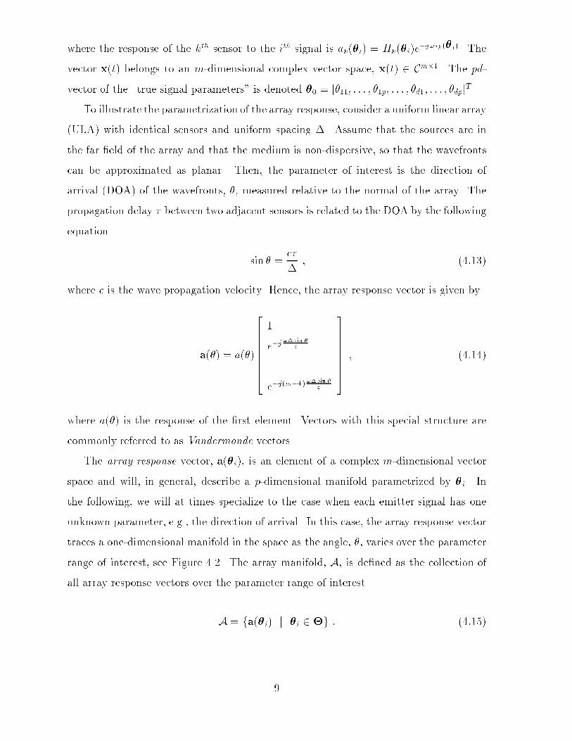
The array response vector� a��i�� is an element of a complex m�dimensional vector

space and will� in general� describe a p�dimensional manifold parametrized by �i� In

the following� we will at times specialize to the case when each emitter signal has one

unknown parameter� e�g�� the direction of arrival� In this case� the array response vector

traces a one�dimensional manifold in the space as the angle� �� varies over the parameter

range of interest� see Figure ���� The array manifold� A� is dened as the collection ofall array response vectors over the parameter range of interest�

A fa��i� j �i � �g � �����

�

a(θ)

Array Manifold

Figure ���� Array manifold�

Let the process x�t� be observed at N time instants� ft�� � � � � tNg� Each vector ob�servation is called a snapshot of the array output and the data matrix is the collection

of the array snapshots

XN �x�t�� � � �x�tN�� A����SN !NN � �����

where the matrices SN and NN are dened analogously to XN �

���� Assumptions and Problem Formulation

The received signal waveforms are assumed to be narrowband� see ������ When deriving

the ML estimator� the following assumptions regarding the statistical properties of the

data are further imposed� The signal� s�ti�� and noise� n�ti�� terms are independent�

zero�mean� complex� Gaussian random processes with second�order moments

Efs�ti�sH�tj�g S ij Efn�ti�nH�tj�g � I ij �����

�

Efs�ti�sT �tj�g � Efn�ti�nT �tj�g � � �����

where ���H denotes complex conjugate transpose� S is the unknown signal covariance

matrix� ij represents the Kronecker delta and I is the identity matrix� In many applica�

tions� the assumption of Gaussian emitter signals is not realistic� A common alternative

model assumes that the emitter signals are unknown deterministic wave forms� see Sec�

tion ��� In the next section� the deterministic �or conditional� model is discussed and

strong justication is provided for why the Gaussian model� which we refer to as the

stochastic model� is appropriate for the signal parameter estimation problem at hand�

The detection and estimation schemes derived from the Gaussian model is found to yield

superior performance� regardless of the actual emitter signals�

As seen from ������ the noise is assumed to be temporally white and also independent

from sensor to sensor� i�e�� spatially white� The noise power is assumed to be identical

in all sensors� and its value� �� is unknown� If the spatial whiteness condition is not

met� the covariance matrix of the noise must be known� e�g� from measurements with

no signals present� In such a case� a whitening transformation is performed on the data�

rendering the transformed noise to be spatially white as described in Section ���

Under the assumptions above the covariance matrix of the measured array output�

referred to as the array covariance� takes the following familiar form

R Efx�ti�xH�ti�g A����SAH���� ! �I � �����

A critical assumption for parameter based array processing techniques is that the func�

tional form of the parametrization of A is known� If the array is carefully designed�

deriving an analytic expression for the array response may be tractable� However� in

most practical applications only array calibration data are available� and the issue of

generating an appropriate array manifold is crucial� It is further required that the man�

ifold vectors are continuously di�erentiable w�r�t� the parameters� and that for any

collection of m distinct �i � �� the matrix �a����� � � � �a��m�� has full rank� An array

satisfying the latter assumption is said to be unambiguous� Due to the Vandermonde

structure of a��� in the ULA case� it is simple to show that the ULA is unambiguous if

the parameter set is � ������ �����

With these preliminaries the sensor array problem can now be formulated as follows�

Given the observations XN and a model for the array response a��i�� estimate

the number of incoming signals d� the signal parameters ��� the signal covariance

matrix S �or alternatively the waveforms SN� and the noise variance ��

The emphasis here is on the estimation of d and ��� Estimation of the other unknowns

is only brie�y discussed� Detailed treatments on the estimation of S is given in ���� and

����� whereas estimation of SN is the subject of �����

��� Parameter Identi�ability

Under the assumption of independent Gaussian distributed observations� all information

in the measured data is contained in the second�order moments� The question of pa�

rameter identiability is thus reduced to investigating under what conditions the array

covariance uniquely determines the signal parameters� Let � represent the unknown

parameters of the covariance R� It is assumed that no a priori information on the signal

covariance is available� Noting that S is a Hermitian matrix� � contains the following

d� ! pd ! real parameters

� h���� � � � � �dp� s��� � � � � sdd� �s��� #s��� � � � � �sd�d��� #sd�d���

�iT

� ������

where �sij Refsijg and #sij Imfsijg� Let R� and R� be two covariance matrices

associated with the parameter vectors �� and ��� and let A�� A� and S�� S� be the

corresponding response matrices and emitter covariances� We will distinguish between

system identi�ability �SI�

R� R� �� �A� A� and S� S�� � �����

and unambiguous parametrization �UP�

�A� A� and S� S�� �� �� �� � ������

�

The problem is parameter identiable �PI�� i�e��

R� R� �� �� �� ���� �

if and only if it is both SI and UP� Let A� and A� be two m d matrices of full rank�

whereas S� and S� are arbitrary d d matrices� Consider the relation

A�S�AH� ! �� I A�S�A

H� ! �� I � ������

If the number of signals is less than the dimension of x�ti�� i�e� d m� then ������

implies �� �� since the smallest eigenvalue of the two covariances must be equal� It

also follows that the matrices S� and S� have the same rank� denoted d�� In the case of

coherent signals �specular multipath or �smart jamming��� the emitter covariance matrix

is singular� i�e�� d� is strictly less than d� Let

Si LiLHi � i � � ������

denote the Cholesky factorization of Si� where Li� i � � are d d� matrices of full

rank� Clearly� ������ is equivalent to

A�L� A�L�L� � ������

for some d� d� unitary matrix L�� In ����� it is shown that a su�cient condition for

������ to imply A� A� �subject to the order of the columns� and� hence� S� S� is

that

d �m! d���� � ������

By assuming an unambiguous array� ������ is trivially satised and we conclude that

the problem is PI� Notice that the requirement that �a����� � � � �a��m�� has full rank for

distinct signal parameters is problem�dependent and� therefore� has to be established for

the specic array under study�

It has been recently shown in ���� that the condition ������ is not only su�cient but

also essentially necessary for PI� Note that if ������ is replaced by the weaker condition

d �d�m���d� ! p�� then PI is guaranteed except for a set of parameter values having

zero measure� see ����� Thus� the latter condition guarantees what is commonly called

generic parameter identiability� However� the concept of generic identiability is of

limited practical value� since for a non�zero measure set of scenarios with parameters

close to the non�identiable set� the accuracy of any parameter estimator will be very

poor� ����� Hence� we will assume in the following that ������ is satised�

�

��� Exact Maximum Likelihood Estimation

The Maximum Likelihood �ML� method is a standard technique in statistical estimation

theory� To apply the ML method� the likelihood function �see e�g� ���� ��� of the observed

data has to be specied� The ML estimates are calculated as the values of the unknown

parameters that maximize the likelihood function� This can be interpreted as selecting

the set of parameters that make the observed data most probable�

When applying the ML technique to the sensor array problem� two main methods

have been considered� depending on the model assumption on the signal waveforms�

When the emitter signals are modeled as Gaussian random processes� a stochastic ML

�SML� method is obtained� see also Sections ����� and ��� If on the other hand the

emitter signals are modeled as unknown deterministic quantities� the resulting estima�

tor is referred to as the deterministic �or conditional� ML �DML� estimator� see also

Sections �� � and ���

���� The Stochastic Maximum Likelihood Method

In many applications it is appropriate to model the signals as stationary stochastic pro�

cesses� possessing a certain probability distribution� The by far most commonly advo�

cated distribution is the Gaussian one� Not only is this for the mathematical convenience

of the resulting approach� but the Gaussian assumption is also often motivated by the

Central Limit Theorem�

Under the assumptions of Section ���� � the observation process� x�ti�� constitutes a

stationary� zero�mean Gaussian random process having second�order moments

Efx�ti�xH�tj�g R ij �A���SAH��� ! � I

ij ������

Efx�ti�xT �tj�g � � ������

In most applications� no a�priori information on the signal covariance matrix is available�

Since S is a Hermitian matrix� it can be uniquely parametrized by d� real parameters�

namely the real diagonal elements and the real and imaginary parts of the lower �or

�

upper� o��diagonal entries� cf� ������� Other possible assumptions are that S is com�

pletely known or unknown but diagonal �uncorrelated signals�� Herein� �� S and � are

all considered to be completely unknown� resulting in a total of d� ! pd ! unknown

parameters�

The likelihood function of a single observation� x�ti�� is

pi�x�

�mjRje�xHR��x � ��� ��

where jRj denotes the determinant of R� This is the complex m�variate Gaussian dis�

tribution� see e�g� ����� Since the snapshots are independent and identically distributed�

the likelihood of the complete data set x�t��� � � � �x�tN� is given by

p�x�t��� � � � �x�tN�j��S� ��

NYi��

�mjRje�xH�ti�R��x�ti� � ��� �

Maximizing p��� ��S� is equivalent to minimizing the negative log�likelihood function�

� log�p��� ��S�

�

NXi��

log

�mjRje�xH�ti�R��x�ti�

�

mN log � ! N log jRj!NXi��

xH�ti�R��x�ti� � ��� ��

Ignoring the constant term and normalizing by N � the SML estimate is obtained by

solving the following optimization problem�

�$�� $S� $�� arg min��S���

l���S� �� � ��� �

where the criterion function is dened as

l���S� �� log jRj!

N

NXi��

xH�ti�R��x�ti� � ��� ��

By well�known properties of the trace operator� Trf�g� the normalized negative log�likelihood function can be expressed as

l���S� �� log jRj! TrfR�� $Rg� ��� ��

�For a scalar a� Trfag � a� and for matricesA andB of appropriate dimensions� TrfABg � TrfBAg

and TrfAg� TrfBg � TrfA�Bg�

�

where $R is the sample covariance

$R

N

NXi��

x�ti�xH�ti� � ��� ��

With some algebraic e�ort the ML criterion function can be concentrated with re�

spect to S and � ���� ��� � �� thus� reducing the dimension of the required numerical

optimization to pd� The SML estimates of the signal covariance matrix and the noise

power are obtained by inserting the SML estimates of � in the following expressions

$S��� Ay���� $R� $���� I�AyH��� ��� ��

$����

m� dTrfP�

A��� $Rg � ��� ��

where Ay is the pseudo�inverse of A and P�Ais the orthogonal projector onto the null

space of AH � i�e�

Ay �AHA���AH ��� ��

PA AAy ������

P�A I�PA � �����

The concentrated form of the SML criterion is now obtained by substituting ��� ���

��� �� into ��� ��� The signal parameter estimates are obtained by solving the following

optimization problem

$� argmin�

VSML��� ������

VSML��� log���A���$S���AH��� ! $���� I

��� � ���� �

Remark ��� It is possible to include the obvious a�priori information that S is positive

semidenite� Since ��� �� may be indenite� this yields potentially a di�erent ML esti�

mator� see ����� In general� if the rank of S is known to be d�� a di�erent parametrization

should be employed� for instance� S LLH� where L is a d d� �lower triangular�

�

matrix� If d� d� these possible modications will have no e�ect for �large enough N��

since ��� �� is a consistent estimate of S� Even if d� d� it can be shown that the asymp�

totic �for large N� statistical properties of the SML estimate cannot be improved by the

square�root parametrization� Since the latter leads to a signicantly more complicated

optimization problem� the unrestricted parametrization of S appears to be preferable�

We will therefore always refer to the minimizer of ���� � as being the SML estimate of

the signal parameters� �

Although the dimension of the parameter space is reduced substantially� the form

of the resulting criterion function ���� � is complicated and the minimizing � can� in

general� not be found analytically� In Section ���� a numerical procedure is described for

carrying out the required optimization�

���� The Deterministic ML Method

In some applications� for example radar and radio communication� the signal waveforms

are often far from being Gaussian random variables� The deterministic model is then

a natural one� since it makes no assumptions at all on the signals� Instead s�ti�� i

� � � � � N are regarded as unknown parameters that have to be estimated� In fact� in some

applications� such as microwave communications� estimation of s�ti� is of more interest

than estimation of �� The ML estimator for this model is termed the DML method�

Similar to the stochastic signal model� the observation process� x�ti�� is Gaussian

distributed given the unknown quantities� The rst� and second�order moments are

di�erent though�

Efx�ti�g A���s�ti� ������

En�x�ti�� Efx�ti�g��x�tj�� Efx�tj�g�H

o �I ij ������

En�x�ti� � Efx�ti�g��x�tj�� Efx�tj�g�T

o � � ������

The unknown parameters are in this case� �� s�ti�� i � � � � � N � and ��

The joint probability distribution of the observations is formed by conditioning on

the parameters of the deterministic model� the signal parameters� the noise variance�

�

and the waveforms� As the snapshots are independent� the conditional density is given

by

p�x�t�� � � �x�tN�j�� ��SN� NYi��

j��Ije�����x�ti��A���s�ti��

H

�x�ti��A���s�ti�� � ������

and the negative log likelihood function has the following form

�log�p��� ��SN�� Nm log���� ! ��Trn�XN �A���SN�

H�XN �A���SN�o

Nm log���� ! ��kXN �A���SNk�F � ������

where k � kF is the Frobenius norm of a matrix� and XN and SN are dened in ������

The deterministicmaximum likelihood estimates are the minimizing arguments of �������

For xed � and SN � the minimum with respect to � is readily derived as

$�

mTrfP�

A��� $Rg � ������

Substituting ������ into ������ shows that $� and $SN are obtained by solving the non�

linear least�squares problem

�$�� $SN � arg min��SN

kXN �A���SNk�F � ������

Since the above criterion function is quadratic in the signal waveform parameters� it

is easy to minimize with respect to SN � see ���� � � ���� This results in the following

estimates

$SN Ay���XN �����

$� arg min�

VDML��� ������

VDML��� TrfP�A��� $Rg � ���� �

�The Frobenius norm of a matrix is given by the square root of the sum of the squared moduli of

the elements�

�

Comparing ���� � and ���� �� we see that the DML criterion depends on � in a simpler

way than does the SML criterion� It is� however� important to note that also �������

���� � is a non�linear multidimensional minimization problem� and the criterion function

often possesses a large number of local minima�

���� Bounds on the Estimation Accuracy

In any practical application involving the estimation of signal parameters� it is of utmost

importance to assess the performance of various estimation procedures� However� any

accuracy measure may be of limited interest unless one has an idea of what the best

possible performance is� An important measure of how well a particular method performs

is the covariance matrix of the estimation errors� Several lower bounds on the estimation

error covariance are available in the literature� see e�g�� � ���������� Of these� the Cram�er�

Rao Lower Bound �CRLB� is by far the most commonly used� The main reason for this

is its simplicity� but also the fact that it is often �asymptotically� tight� i�e�� there exists

an estimator that �asymptotically� achieves the CRLB� Such an estimator is said to be

�asymptotically� e�cient� Unless otherwise explicitly stated� the word �asymptotically�

is used throughout this chapter to mean that the amount of data �N� is large�

Theorem ��� Let $� be an unbiased estimate of the real parameter vector ��� i�e��

Ef$�g ��� based on the observations XN � The Cramer�Rao lower bound on the es�

timation error covariance is then given by

Ef�$� � ����$� � ���Tg

�E

�� log p�XN j��

����T

����� ������

�

The matrix within square brackets in ������ �i�e�� the inverse of the CRLB� is referred

to as the Fisher Information Matrix �FIM��

The Cram�erRao Lower Bound

The CRLB based on the Gaussian signal model is discussed� for example in ��� ���� and

is easily derived from the normalized negative log likelihood function in ��� ��� Let �

��

represent the vector of unknown parameters in the stochastic model

� h�T � s��� � � � � sdd� �s��� #s��� � � � � �sd�d��� #sd�d���

�iT

� ������

where �sij Refsijg and #sij Imfsijg� Introduce the short hand notation

Ri �R

��i������

and recall the following di�erentiation rules ����

�

��ilog jRj TrfR��Rig ������

�

��iTrfR�� $Rg �TrfR��RiR

�� $Rg � ������

������

The rst derivative of ��� �� with respect to the ith component of the parameter vector

is given by

�l���

��i TrfR��Ri�I�R�� $R�g� ������

The following then gives the ijth element of the inverse of the CRLB

fFIMgij N E

��l���

��j��i

���������

�

N EnTrh��R���jRi !R

��Rij

�I�R�� $R

�R��Ri�R

���j $Rio

N EnTrh�R��Ri�R

���j $Rio

N TrnR��RiR

��Rj

o� �����

The appearance of N on the right hand side above is due to the normalization of ��� ���

In many applications� only the signal parameters are of interest� However� the above

formula involves derivatives with respect to all d� ! pd ! components of �� and in

general none of the elements of ����� vanish� A compact expression for the CRLB on

�

the covariance matrix of the signal parameters only is presented in ���� �� ���� The

Cram�er�Rao inequality for � is given by

Ef�$� � ����$� � ���Tg BSTO � ������

where

fB��STOgij

�N

�Re

hTrnAH

j P�AAiSA

HR��ASoi

i� j � � � � � pd � ���� �

For the special case when there is one parameter associated with each signal �p ��

the CRLB for the signal parameters can be put in a simple matrix form

BSTO �

�N

hRe

n�DHP�

AD�� �SAHR��AS�Toi��

� ������

where � denotes the Hadamard �or Schur� product� i�e�� element�wise multiplication�

and

D

�� �a�����

���������

� � � � ��a���

��

��������d

�� � ������

The Deterministic Cram�erRao Lower Bound

The CRLB for deterministic signals is derived in � �� �� and is restated here in its

asymptotic form� and for the case p � The emitter signals are arbitrary second�order

ergodic sequences� and with some abuse of notation� the limiting signal sample covariance

matrix is denoted

S limN��

N

NXi��

s�ti�sH�ti� � ������

If the signal waveforms happen to be realizations of stationary stochastic processes� the

limiting signal sample covariance will indeed coincide with the signal covariance matrix

under mild assumptions �e�g�� bounded fourth�order moments��

Let $� be an asymptotically unbiased estimate of the true parameter vector ��� For

large N � the Cram�er�Rao inequality for the signal parameters can then be expressed as

Ef�$� � ����$� � ���Tg BDET � ������

��

where

fB��DETgij

�N

�Re

hTrnAH

j P�AAiS

oi� ������

It should be noted that the above inequality assumes implicitly that asymptotically

unbiased estimates of all unknown parameters in the deterministic model� i�e�� ��SN and

� are available� No assumptions on the signal waveforms are� however� made so the

inequality applies also if they happen to be realizations of Gaussian processes� One may

therefore guess that BSTO is tighter than BDET � We shall prove this statement later in

this section�

��� Asymptotic Properties of the ML Estimates

The ML estimator has a number of attractive properties that hold for general� su�ciently

regular� likelihood functions� The most interesting one for our purposes states that if

the ML estimates are consistent� then they are also asymptotically e�cient� In this

respect� the ML method has the best asymptotic properties possible�

Stochastic Maximum Likelihood

The SML likelihood function is regular and the general theory of ML estimation can be

applied to yield the following result�

Theorem ��� Under the Gaussian signal assumption� the SML parameter estimates are

consistent and the normalized estimation error�pN �$� � ���� has a limiting zero�mean�

normal distribution with covariance matrix equal to N times the CRLB on $��

Proof See for example Chapter ��� in ���� for a proof� �

From the above we conclude that for the SML method� the asymptotic distribution ofpN�$� � ��� is N���CSML�� where

CSML N BSTO � ������

and where BSTO is given by ���� ��

�An estimate is consistent if it converges to the true value as the amount of data tends to in�nity�

�

Deterministic Maximum Likelihood

The deterministic model for the sensor array problem has an important drawback� Since

the signal waveforms themselves are regarded as unknown parameters� it follows that

the dimension of the parameter vector grows without bound with increasing N � For this

reason� consistent estimation of all model parameters is impossible� More precisely� the

DML estimate of � is consistent� whereas the estimate of SN is inconsistent� To verify

the consistency of $�� observe that under mild conditions� the criterion function ���� �

converges w�p� and uniformly in � to the limit function

�VDML��� TrnP�A���R

o Tr

nP�A���

�A����SA

H���� ! �Io

������

as N tends to innity� Hence� $� converges to the minimizing argument of �VDML���� It

is readily veried that �VDML��� �TrfP�A���g ��m� d� �V ���� �recall that the

trace of a projection matrix equals the dimension of the subspace onto which it projects��

Let S LLH be the Cholesky�factorization of the signal covariance matrix� where L is

d d�� Clearly �VDML��� ��m� d� holds if and only if P�A���A����L �� in which

case

A���L� A����L � �����

for some d d� matrix L� of full rank� By the UP assumption and ������� the relation

����� is possible if and only if � ��� Thus� we conclude that the minimizer of ���� �

converges w�p� to the true value ���

The signal waveform estimates are� however� inconsistent since

$SN Ay�$��XN �� SN !Ay����NN as N � � ������

Owing to the inconsistency of $SN � the general properties of ML estimators are not valid

here� Thus� as observed in � ��� the asymptotic covariance matrix of the signal parameter

estimate does not coincide with the deterministic CRLB� Note that the deterministic

Cram�er�Rao inequality ������ is indeed applicable� as the DML estimate of SN can be

shown to be asymptotically unbiased �with some e�ort� in spite of its inconsistency�

��

The asymptotic distribution of the DML signal parameter estimates is derived in

� �� ��� and is given next for the case of one parameter per emitter signal�

Theorem �� Let $� be obtained from ������ Then�pN�$�� ��� converges in distribu�

tion to N���CDML�� where

NCDML BDET ! �N BDETRe

n�DHP�

AD�� �AHA��ToBDET � ���� �

where BDET is the asymptotic deterministic CRLB as de�ned in �� ���

From ���� �� it is clearly seen that the covariance of the DML estimate is strictly greater

than the deterministic CRLB� However� these two matrices approach the same limit as

the number of sensors� m� increases� see � ��� The requirement of the DML method to es�

timate the signal waveforms has thus a deteriorating e�ect on the DOA estimates� unless

m is large� In many applications the signal waveform estimates may be of importance

themselves� Though the DML technique provides such estimates� it should be remarked

that they are not guaranteed to be the most accurate ones� unless m is large enough�

���� Order Relations

As discussed above� the two models for the sensor array problem� corresponding to deter�

ministic and stochastic modeling of the emitter signals respectively� lead to di�erent ML

criteria and CRLB�s� The following result� due to � �� ��� relates the covariance matrices

of the stochastic and deterministic ML estimates and the corresponding CRLB�s�

Theorem ��� Let CSML and CDML denote the asymptotic covariances ofpN�$� �

���� for the stochastic and deterministic ML estimates� respectively� Furthermore� let

BSTO and BDET be the stochastic CRLB and the deterministic CRLB� The following

�in�equalities then hold

NCDML

NCSML BSTO BDET � ������

Proof Theorem ��� shows the middle equality above� The left inequality follows by

applying the DML method under the Gaussian signal assumption� The Cram�er�Rao

��

inequality then implies that N��CDML BSTO� To prove the right inequality in �������

apply the matrix inversion lemma �e�g�� ��� Lemma A�� to obtain

SAHR��AS S� S�I�AH�ASAH ! �I���AS

S� S

�I!AH��AS

��� ������

Since the matrix S�I!AH��AS��� is Hermitian �by the equality above� and positive

semi�denite� it follows that SAHR��AS � S� Hence� application of � ��� Lemma A���

yields

Ren�DHP�

AD�� �SAHR��AS�To� Re

n�DHP�

AD�� STo

������

By inverting both sides of ������� the desired inequality follows� If the matricesDHP�AD

and S are both positive denite� the inequality ������ is strict showing that the stochastic

bound is in this case strictly tighter than the deterministic bound� �

Remark ��� It is of course natural that the SML estimator is more accurate than the

DML method under the Gaussian signal assumption� However� this relation remains

true for arbitrary second�order ergodic emitter signals� which is more surprising� This

is a consequence of the asymptotic robustness property of both ML estimators� the

asymptotic distribution of the signal parameter estimates is completely specied by

limN����N�PN

i�� s�ti�sH�ti�� As shown in � �� ���� the actual signal waveform sequence

�or its distribution� is immaterial� The fact that the SMLmethod always outperforms the

DML method� provides strong justication for the stochastic model being appropriate

for the sensor array problem� Indeed� the asymptotic robustness and e�ciency of the

SML method implies that N BSTO CSML is a lower bound on the covariance matrix

of the normalized estimation error for any asymptotically robust method� �

��

��� Large Sample ML Approximations

The previous section dealt with optimal �in the ML sense� approaches to the sensor array

problem� Since these techniques are often deemed exceedingly complex� suboptimal

methods are of interest� In the present section� several subspace techniques are presented

based on geometrical properties of the data model�

The focus here is on subspace based techniques where the vector of unknown signal

parameters is estimated by performing a multidimensional search on a pd�dimensional

criterion� This is in contrast to techniques such as the MUSIC algorithm ��� �� where

the location of d peaks in a p�dimensional so�called spatial spectrum determines the signal

parameter estimates� Multidimensional versions of the MUSIC approach are discussed in

���� � ��� � �� A multidimensional subspace based technique termed MODE �method of

direction estimation� is presented and extensively analyzed in � �� �� ���� In ���� ��� ����

a related subspace tting formulation of the sensor array problem is analyzed and the

WSF �weighted subspace tting� method is proposed�

This section ties together many of the concepts and methods presented in the papers

above and discusses the relation of these to the ML techniques of the previous section� A

statistical analysis shows that appropriate selections of certain weighting matrices give

the subspace methods similar �optimal� estimation accuracy as the ML techniques� at a

reduced computational cost�

��� The Subspace Based Approach

All subspace based methods rely on geometrical properties of the spectral decomposition

of the array covariance matrix� R� The early approaches such as MUSIC su�er from a

large nite sample bias and are unable to cope with coherent signals�� This problem is

inherent due to the one�dimensional search �p�dimensional search when more than one

parameter is associated with each signal� of the parameter space� Means of reducing

the susceptibility of these techniques to coherent signals have been proposed for special

array structures� see e�g� ����� In the general case� methods based on a pd�dimensional

search need to be employed�

�Two signals are said to be coherent if they are identical up to amplitude scaling and phase shift�

��

If the signal waveforms are non�coherent� the signal covariance matrix� S� has full

rank� However� in radar applications where specular multipath is common� S may be

ill�conditioned or even rank decient� Let the signal covariance matrix have rank d�� The

covariance of the array output is

R A����SAH���� ! �I � ������

It is clear that any vector in the null space of the matrix ASAH is an eigenvector of R

with corresponding eigenvalue �� Since A has full rank� ASAH is positive semi�denite

and has rank d�� Hence� � is the smallest eigenvalue of R with multiplicitym� d�� Let

��� � � � � �m denote the eigenvalues of R in non�increasing order� and let e�� � � � � em be the

corresponding orthonormal eigenvectors� The spectral decomposition of R then takes

the form

R mXi��

�ieieHi Es�sE

Hs ! �EnE

Hn � ������

where

�s diag���� � � � � �d�� � Es �e�� � � � � ed�� � En �ed���� � � � � em� � ������

The diagonal matrix �s contains the so�called signal eigenvalues� and these are assumed

to be distinct� From the above discussion� it is clear that En is orthogonal to ASAH �

which implies that the d��dimensional range space of Es is contained in the d�dimensional

range space of A����

�fEsg � �fA����g � ������

If the signal covariance S has full rank� these subspaces coincide since they have the same

dimension� d� d� The range space of Es is referred to as the signal subspace and its

orthogonal complement� the range space of En� is called the noise subspace� The signal

and noise subspaces can be consistently estimated from the eigendecomposition of the

sample covariance

$R

N

NXi��

x�ti�xH�ti� $Es

$�s$EHs ! $En

$�n$EHn � �����

��

Signal Subspace Formulation

The relation in ������ implies that there exists a d d� matrix T of full rank� such that

Es A����T � ������

In general� there is no value of � such that $Es A���T when the signal subspace is

estimated from the noise�corrupted data� With this observation� a natural estimation

criterion is to nd the best weighted least squares �t of the two subspaces� viz�

�$�� $T� arg min��T

k$Es �A���Tk�W� ���� �

where kAk�W TrfAWAHg andW is a d�d� positive denite weighting matrix �to be

specied�� The optimization ���� � is a least�squares problem� which is linear in T and

non�linear in �� Substituting the pseudo�inverse solution� $TLS Ay$Es �see� e�g� ����

Complement C�� � in ���� �� we obtain

$� argmin�

VSSF ��� � ������

where

VSSF ��� k$Es �A���Ay���$Esk�W kfI�PA���g$Esk�W TrfP�

A���$EsW$EHs P

�A���g

TrfP�A���$EsW

$EHs g � ������

The above equations dene the class of subspace tting �SSF� methods� Di�erent mem�

bers in this class correspond to specic choices of weighting matrix in ������� It should

be noted that the choice W I yields Cadzow�s method� �� �� A statistical analysis

suggests other weightings� leading to superior performance as demonstrated later�

��

Noise Subspace Formulation

If the emitter signal covariance� S� has full rank� i�e�� d� d� it is clear that the columns

of A���� are orthogonal to the noise subspace� i�e�

EHn A���� � � ������

When an estimate of the noise subspace is available� a weighted least�squares measure of

orthogonality can be formulated� A natural estimate of � is then obtained by minimizing

that measure

$� argmin�

VNSF ��� � ������

where

VNSF ��� k$EHnA���k�U

Trf$EHn A���UA

H���$Eng TrfUAH���$En

$EHnA���g � ������

where U � is a d d weighting matrix� Di�erent choices of weighting� U� result

in signal parameter estimates with di�erent asymptotic properties� Indeed� if U is a

diagonal matrix� the problem decouples and the MUSIC estimator is obtained� Again�

a statistical analysis suggests other weightings giving better estimation accuracy�

��� Relation Between the Subspace Formulations

The subspace techniques above can be shown to be closely related� Before discussing their

relationship� it is necessary to dene what is meant herein by asymptotic equivalence of

estimators�

De�nition ��� Two estimates� $�� and $��� of the same true parameter vector are asymp�

totically equivalent if

pN�$�� � $���� � ������

in probability as N � �

�

Notice� in particular� that if $�� and $�� are asymptotically equivalent� the asymptotic

distributions of the normalized estimation errorspN �$�� � ��� and

pN�$�� � ��� are

identical� A rst�order Taylor expansion shows that under mild conditions� two consistent

parameter estimates obtained from the minimization of two di�erent functions J��� and

V ��� are asymptotically equivalent if

J ����� V ����� ! op��pN � ������

J ������ V ������ ! op�� � �����

where the symbol op��� represent the �in probability� version of the corresponding de�terministic notation �

The following theorem establishes the relationship between the signal and noise sub�

space formulations� ������ and �������

Theorem �� The estimate obtained by minimizing ����� with weighting matrix given

by

U Ay����$EsW$EHs A

yH����� ������

is asymptotically equivalent to the minimizing argument of ������

Proof To establish ������� consider rst the derivative of ������� Using the formula

�A� � for the derivative of the projection matrix and dening Ai �A���i� we have

�VSSF��i

�Trf�PA��i

$EsW$EHs g

��RehTrnP�AAiA

y$EsW$EHs

oi� ���� �

Next� examine the derivative of the cost function �������

�VNSF

��i �Re

hTrfUAH $En

$EHnAig

i� ������

�A sequence� xN � of random variables is op�aN � if the probability limit of a��N xN is zero�

Inserting the expression for the weighting matrix ������� the argument of the trace above

is

Ay$EsW$EHs A

yHAH $En$EHn Ai �Ay$EsW

$EHs P

�A$En$EHn Ai ������

�Ay$EsW$EHs P

�AEnE

Hn Ai ! op��

pN� ������

�Ay$EsW$EHs P

�AAi ! op��

pN� � ������

In ������� the relations AyHAH PA I � P�Aand $EH

s$En � are used� Noting that

$EHs P

�A Op��

pN� and $En

$EHn EnE

Hn ! op�� leads to ������� Finally� the fact that

P�AEnE

Hn P�

Ais used to obtain ������� Substituting ������ into ������ and comparing

with ���� � shows that ������ is satised�

Consider the second derivative of ������

��VNSF

��i��j �Re

hTrfUAH

i$En$EHn Aig

i! �Re

hTrfUAH $En

$EHnAijg

i� ������

Inserting ������ and evaluating the probability limit as N � � we obtain after somemanipulations

��VNSF

��i��j� �Re

hTrfAjP

�AA

Hi A

yEsWE�sAyHg

i� ������

Using �A���� it is straightforward to verify that the limiting second derivative of ������

coincides with ������� see also ����� �

Note that the weighting matrix in ������ depends on the true signal parameters ���

However� the following lemma shows that the weighting matrix �for both subspace for�

mulations� can be replaced by any consistent estimate thereof without a�ecting the

asymptotic properties� Thus� a two�step procedure can be applied� where �� is replaced

by a consistent estimate as described in ����

Lemma ��� If the weighting matrix W in ����� is replaced by a consistent estimate�

an asymptotically equivalent signal parameter estimate is obtained� If d� d� the same

is true for U in ������

�

Proof Let $W W!op�� and write VSSF �W� to stress its dependence on the weighting

matrix� Examine the derivative in ���� �

�VSSF��i

VSSF�i �W� ��RehTrfAy$EsW

$EHs P

�AAig

i� ������

Since $EHs P

�A Op��

pN �� it readily follows that VSSF�i �W� VSSF�i � $W� ! op��

pN�

which shows ������� Next� assume that d� d and let $U U ! op��� From ������ we

then have VNSF�i �U� VNSF�i � $U�!op��pN�� sinceAH $En

$EHn Op��

pN�� Condition

����� is trivially satised for both criteria� �

This result will be useful when considering di�erent choices of weighting matrices which

are data dependent�

��� Relation to ML Estimation

In the previous section� the subspace based methods are derived from a purely geo�

metrical point of view� The statistical properties of these techniques reveal unexpected

relations to the previously described ML methods� The following result gives the asymp�

totic distribution of the signal parameter estimates obtained using the signal subspace

technique and a general �positive denite� weighting matrix�

Theorem ��� Let $� be obtained from ����������� Then $� converges to the true

value� ��� w�p�� as N tends to in�nity� Furthermore� the normalized estimation error�pN�$� � ���� has a limiting zero�mean Gaussian distribution

pN�$� � ��� � AsN���C� � �����

The covariance of the asymptotic distribution has the form

C H��QH�� � ������

Here� H denotes the limiting Hessian matrix and Q is the asymptotic covariance matrix

of the normalized gradient

H limN��

V ��SSF ���� ���� �

Q limN��

N EfV �SSF ����V

�TSSF ����g � ������

The ijth elements of these matrices are given by

Hij �RehTrnAH

j P�AAiA

yEsWEHs A

yHoi

������

Qij ��Re�TrfAH

j P�AAiA

yEsW�se���

WEHs A

yHg�� ������

where

e� �s � � I � ������

�

Theorem ��� relates the asymptotic properties of the signal and noise subspace formula�

tions� Hence� the above result gives the asymptotic distribution for the latter estimator

as well� provided U is chosen conformally with ������� If d d�� this imposes no restric�

tion and an arbitrary U � � can be chosen� However� in case d� d the relation ������ is

not invertible and Theorem ��� gives the distribution only for U�s having this particular

form�

Some algebraic manipulations of the expression for the asymptotic estimation error

covariance give the following result�

Corollary ���

a� The weightings Wopt e�����s and Uopt Ay����$EsWopt

$EHs A

yH���� result in

estimators which are large sample realizations of the SML method� i�e�� the asymp�

totic distributions of the normalized estimation errors coincide�

b� If d� d� the weightings W e� and U Ay����$Ese�$EH

s AyH���� result in large

sample realizations of the DML method�

�

Proof To prove a�� note that H�Wopt� ��Q�Wopt�� Comparing ������ and ���� ��

it su�ces to verify that

AyEsWoptEHs A

yH SAHR��AS � ������

Equations ������������� imply

Es�sEHs ASAH ! �EsE

Hs � ������

from which it follows that

AyEse�EH

s AyH AyASAHAyH S � �����

Using ����� and the eigendecomposition of R��� we have

SAHR��AS AyEse�EH

s AyHAH

�Es�

��s EH

s ! ��EnEHn

AAyEs

e�EHs A

yH

AyEse����

se�EH

s AyH � ����

since AAyEs PAEs Es�

To establish b�� observe from ������� ������ and ������ that forW e�� H is given

by

H�� N

�BDET � �����

If d� d� ����� gives

AyEs�sEHs A

yH S! ��AHA��� � ��� �

and ������ reads

Qij ��RehTrnAH

j P�AAi�S! ��AHA����

oi

�

N�B��

DET �ij ! ��Re

hTrnAH

j P�AAi�A

HA���oi

� �����

�

Now� combining ������� ����� and ����� leads to the following covariance when the

weighting is chosen asW e� and p

C N BDET ! � N�BDETRe

n�DHP�

AD�� �AHA��ToBDET CDML �����

The last equality follows by comparing with ���� �� �

The result above states that with appropriate choice of weighting matrices� the subspace

based techniques are as accurate as the ML methods� In fact� the corresponding subspace

and ML estimates of the signal parameters are asymptotically equivalent� which is slightly

stronger�

It is interesting to observe that the DML weighting for the noise subspace technique

gives U � AyEse�EH

s AyH S� Thus� we rediscover the fact that MUSIC is a large

sample realization of the DML method if S is diagonal �uncorrelated sources�� Recall

that ������ reduces to MUSIC whenever U is diagonal� The asymptotic equivalence of

MUSIC and the DML method for uncorrelated signals was rst proved in � ��� It should

also be remarked that part b� above is also shown in � ��

It is straightforward to show that the weighting matrix that gives the lowest asymp�

totic estimation error variance is Wopt e�����s � This is not surprising� since the

corresponding estimation error covariance coincides with the stochastic CRLB� The op�

timally weighted signal subspace technique ������ is referred to as the weighted subspace

�tting �WSF� method� Systematic derivations of the method can be found in ����� where

the SML method is approximated by neglecting terms that do not a�ect the asymp�

totic properties� and in ���� ���� where the asymptotic likelihood function of P�A$Es is

considered�

Remark �� The optimally weighted noise subspace technique is obtained by using U

Ay����$EsWopt$EHs A

yH����� However� note that the replacement of �� by a consistent

estimate in this expression does a�ect the asymptotic distribution of $� if d� d� cf� the

requirement d� d in Lemma ��� In fact� one can show that for d� d� the signal

parameter estimates obtained using the optimally weighted noise subspace technique

�

are not asymptotically equivalent with the SML estimates� Modications to the cost

function can be made to obtain equivalence with the SML method� but this results in

an increase in the computational cost when minimizing the criterion function� In the

following we will therefore only consider the WSF cost function� �

�

��� Calculating the Estimates

All methods considered herein require a multidimensional non�linear optimization for

computing the signal parameter estimates� Analytical solutions are� in general� not avail�

able and one has to resort to numerical search techniques� Several optimization methods

have appeared in the array processing literature� including expected maximization �EM�

algorithms ���� ���� the alternating projection �AP� method ����� iterative quadratic ML

�IQML� ����� �global� search techniques ���������� as well as di�erent Newton�type tech�

niques �� � � � ���� �� ������� In this section� Newton�type algorithms for the SML� DML

and WSF techniques are described� For the special case of a uniform linear array� a

non�iterative scheme for the subspace�based method is presented�

���� Newton Type Search Algorithms

Assume that V ��� is a continuously di�erentiable function� whose minimizer� $�� is to be

found� One of the most e�cient optimization methods for such problems is the damped

Newton method ���� ���� The estimate is iteratively calculated as

�k�� �k � �kH��V �� �����

where �k is the estimate at iteration k� �k is the step length� H represents the Hessian

matrix of the criterion function� and V � is the gradient� The Hessian and gradient are

evaluated at �k� It is well�known that the Newton method gives locally a quadratic

convergence to $��

The step length� �k� should be appropriately chosen in order to guarantee convergence

to a local minimum� An often used scheme for Newton methods is to choose some �

and to take �k ���i for the smallest integer i � that causes �su�cient decrease�

in the criterion function� The reader is referred to ���� and ���� for more sophisticated

algorithms for selecting the step length� A useful modication of the damped Newton

method� particularly suited for ill�conditioned problems� is to use �H! �kI��� in lieu of

�kH��� where �k is increased from � until a decrease in the criterion function is observed�

This� in combination with the Gauss�Newton modication of the Hessian ���� ��� for non�

linear least squares problems� is referred to as the Levenberg�Marguardt technique�

�

The iterations ����� continue until some prescribed stopping criterion is satised�

Examples of such criteria are�

� jH��V �j is less than a specied tolerance and H � ��

� no improvement can be found along the search direction ��k smaller than a toler�ance��

� the number of iterations reaches a maximum limit�

The quality of the convergence point depends on the shape of the criterion function in

question� If V ��� possesses several minima� the iterations must be initialized �su�ciently

close� to the global minimum in order to prevent convergence to a local extremum�

Possible initialization schemes will be discussed in Section ������

���� Gradients and Approximate Hessians

The idea behind Newton�s method is to approximate the criterion function locally around

the stationary point by a quadratic function� The role of the Hessian can be seen

as a modication of the gradient direction� to take into account the curvature of the

approximation� The Newton method has some drawbacks when applied to the problems

of interest herein� Firstly� while the negative gradient is� by denition� a descent direction

for the criterion function� the Newton�direction ��H��V �� can be guaranteed to be

a descent direction only if H is positive denite� This may not be the case further

away from the minimum� where V ��� cannot� in general� be well�approximated by a

quadratic function� Hence� there may be no value of �k that causes a decrease in the

criterion� Secondly� the evaluation of the exact Hessian matrices for the SML� DML�

and WSF criteria is computationally cumbersome� A standard technique for overcoming

these di�culties is to use a less complex approximation of the Hessian matrix� which

is also guaranteed to be positive semidenite� The techniques to be described use the

asymptotic �for large N� form of the Hessian matrices� obtained from the previously

described asymptotic analysis� In the statistical literature� this is often referred to as

the scoring method� It is closely related to the Gauss�Newton technique for non�linear

least squares problems� It is interesting to observe that for the SML and WSF methods�

the inverse of the limitingHessian coincides �to within a scale factor� with the asymptotic

�

covariance matrix of the estimation errors� Consequently� an estimate of the accuracy is

readily available when the optimum is reached�

In the following� expressions for the gradients and the approximate Hessians are

presented for the methods in question� To keep the notation simple� we shall specialize

to the case of one parameter per source� i�e�� p � The extension to a general p is

straightforward�

Stochastic Maximum Likelihood

The SML cost function is obtained from ���� �� Evaluation of this expression requires

O�m�� complex �oating point operations ��ops�� Making use of the determinant rule

jI ! ABj jI !BAj �see e�g� ���� Appendix A� to rewrite ���� �� the computationalcost can be reduced to O�m�d� �ops as follows�

VSML��� log���A$S���AH ! $����I

��� log $�m���

���$�����$S���AHA ! I���

log $��m�d�������Ay $RA

��� � �����

where� in the last equality� we have used ��� ������ ���

Next� introduce the matrix

G Ah�AH $RA��� � $������AHA���

i� �����

The SML gradient can then be expressed as � ���

V �SML��� �Re

�Diag

hGH $RP�

ADi

� �����

where the matrix D is dened in ������ and the notation Diag�Y�� where Y is a square

matrix� means a column vector formed from the diagonal elements of Y� The approxi�

mate Hessian is obtained from the CRLB� From ������ we have

HSML��� �

�Re

n�DHP�

AD�� �SAHR��AS�T

o� ������

��

Replacing the unknown quantities S and � by their SML estimates ��� ������ �� and

R by A$S���AH ! $���� I in ������� leads after some manipulations to

$S���AH�A$S���AH ! $���� I

��A$S��� $����GH $RG � �����

Inserting ����� into ������ yields the asymptotic Hessian matrix

HSML �$����Re

n�DHP�

AD�� �GH $RG�To� ������

Deterministic Maximum Likelihood

The DML cost function is given by ���� �

VDML��� TrfP�A��� $Rg � ���� �

Di�erentiation with respect to � gives the gradient expression � �� ����

V �DML��� ��Re

nDiag�Ay $RP�

AD�o� ������

The asymptotic DML Hessian is derived in � �� ���

HDML �Ren�DHP�

AD�� STo� ������

A di�culty when using the above is that the DML method does not explicitly provide

an estimate of the signal covariance matrix� One could construct such an estimate from

the estimated signal waveforms ����� as

$$S

N$SN $S

HN Ay $RAyH � ������

Using this in ������ results in the modied Gauss�Newton method� as suggested in �����

However� ������ does not provide a consistent estimate of S� Thus� we propose here to

use the corresponding SML estimate ��� �� in ������ to give

HDML �Re��DHP�

AD��hAy� $R� $����I�AyH

iT�� ������

�

Subspace Fitting Criterion

The WSF cost function is given by �������

VWSF ��� TrfP�A$Es$Wopt

$EHs g � ������

where the data dependent weighting matrix

$Wopt �$�s � $�I�� $���

s ������

is used� Here� $� refers to a consistent estimate of the noise variance� for example the

average of the m � d� smallest eigenvalues of $R� Observe the similarity of ������ and

the DML criterion ���� �� The rst derivative is immediate from ������

V �WSF ��� ��Re

nDiag

hAy $Es

$Wopt$EHs P

�AD

io� ��� ��

The asymptotic expression for the WSF Hessian is obtained from ������ as

HWSF �Ren�DHP�

AD�� �Ay$Es$Wopt

$EHs A

yH�To� ��� �

It is interesting to observe that the scoring method for the WSF technique coincides with

the modied Gauss�Newton method used in �����

���� Uniform Linear Arrays

For the special case where the array elements are identical and equidistantly spaced

along a line� and p � the subspace�based method� ������� can be implemented in a

non�iterative fashion� ��� ����

This simplication is based on a reparametrization of the loss function in terms of

the coe�cients of the following polynomial

b�z� b�zd ! b�z

d�� ! � � �! bd b�dY

k��

�z � e�j�� sin �k�c� � ��� ��

��

Thus� the signal parameters can easily be extracted from the roots of the polynomial

once the latter is available� The array propagation matrix has a Vandermonde structure

in the ULA case� see ������ Dening �k ��"sin �k�c� we have

A���

����������

� � �

ej�� � � � ej�d

���� � �

���

ej�m����� � � � ej�m����d

����������� ��� �

Introduce the m �m� d� matrix B

BH

�������bd bd�� � � � b� �

� � � � � � � � �

� bd bd�� � � � b�

������� � ��� ��

and observe that

BHA � � ��� ��

Since B has rank �m� d�� it follows that B spans the null space of AH � i�e��

P�A PB B�BHB���BH � ��� ��

Hence� ������ can be rewritten in terms of the polynomial coe�cients as

V ��� TrnB�BHB���BH $EsW

$EHs

o� ��� ��

Since BH $Es is of order Op��pN� locally around the �true� B� it can easily be shown

that the term �BHB��� in ��� �� can be replaced by any consistent estimate without

a�ecting the asymptotic properties of the minimizing B� This observation leads to the

minimization of the function

TrnB� $BH $B���BH $EsW

$EHs

o Tr

n� $BH $B���BH $EsW

$EHs B

o� ��� ��

�

which is quadratic in B� A consistent initial estimate of B is obtained� for example by

using $BH $B I above� Some care must be exercised concerning the constraint on the

polynomial coe�cients� all roots of b�z� should lie on the unit circle� This constraint is

extensively discussed in ��� ���� and an algorithm for minimizing ��� �� involving only

the solution of a linear system of equations is proposed�

��� Practical Aspects

In this section� the computational requirements for obtaining the various estimates are

brie�y discussed� A detailed implementation of the scoring method for the WSF algo�

rithm is given�

Initial Data Treatment

The computational complexity of an algorithm depends clearly on the application and the

availability of parallel processors� For sequential batch processing� and for N � m� it is

clear that the computational cost is dominated by forming the sample covariance ��� ���

which takesNm� �ops� However� most applications involve the tracking of a time�varying

scenario� The sample covariance is then recursively updated� at a high rate �preferably

using parallel processing�� and estimates of $R are delivered to the estimation routine at a

relatively low rate� This is because the scenario varies usually rather slowly as compared

to the sampling rate� To be able to track time�variations� the sample covariance estimate

$R could be reset to zero after each delivery� or alternatively a forgetting factor �e�g��

���� Chapter �� could be used when forming $R� The speed at which signal parameter

estimates must be calculated is clearly related to how quickly the scenario is changing�

The subspace�based methods require the eigenvalues and the d� principal eigenvec�

tors of $R� The signal subspace dimension� d�� is typically determined by testing the

multiplicity of the smallest eigenvalue of $R ���� ��� ���� See also Chapters � and � A

standard routine for calculating the required eigendecomposition costs approximately

�m� �ops ���� However� much attention has recently been paid to utilize the structure

It is numerically more reliable to update the Cholesky factor of the sample covariance to avoid

squaring the data� see e�g�� ����

��

of R to reduce this cost� In ����� a �batch�type� procedure for computing an approxi�

mation of the eigendecomposition is proposed� The referenced technique requires O�m��

operations and includes a scheme for estimating d�� Fast algorithms for updating the

signal subspace after a rank�one modication of $R �i�e�� after collecting one additional

snapshot� are discussed in� e�g�� �� �������

Estimator Implementation

Given the sample covariance or its eigendecomposition� an iteration of the scoring method

involves the evaluation of the current values of the criterion function V � gradient V ��

approximate Hessian H� and search direction� s �H��V ��

All techniques require the calculation of Ay and P�A� This is best done by QR�

decomposition of A using� for example� Householder transformations ���

A QR �Q��Q��

��� R�

�

��� �

Ay R��� QH

� � P�A Q�Q

H� �

Performing a QR�decomposition using Householder transformations requires d��m�d� �operations� The matrix Q is stored as a product of Householder transformations� which

allows forming QHx� where x is an m�vector� with O�md� �ops� see ����

We shall describe a detailed implementation of the WSF�scoring method� For the

stochastic and deterministic ML techniques� only an approximate operation count is

presented� The eigendecomposition of $R is assumed available� as well as A and D� as

evaluated at the current iterate�

��

WSFscoring implementation

� Weighted signal subspace matrix

M $Es� $�s � $�I� $�����

s �

where $� �Pm

i�d���$�i���m� d���

� QR�decomposition using Householder transformations

A �Q��Q��

��� R�

�

���

� Intermediate variables

� QH� D� � MHQ�� � R��

� QH� M

� Criterion function� gradient� and Hessian

V Trf��HgV � ��RefDiag�����gH �Ref��H��� ���H�Tg

� Search direction� Solve Hs �V �

The above scheme takes about md�! �mdd� !O�d�� �ops� Similar implementations of

the SML� and DML�scoring techniques require each approximately � d!�m�!�md�!

O�d�� �ops per iteration� When m � d� as is common in radar applications� the WSF

iterations can thus be implemented using signicantly less operations than the SML and

DML methods�

��

Initialization

For the Newton type techniques discussed above� initialization is of course a crucial issue�

A natural way to obtain initial estimates is to use a �consistent� suboptimal estimator�

When the array has a special invariance structure� the Total Least Squares �TLS� version

of the ESPRIT algorithm� ���� is an attractive choice� This algorithm is applicable to any

array that consists of two identical subarrays� For more general array geometries� the

MUSIC algorithm ��� � could be used� An important drawback of most suboptimal

techniques is the severe degradation of the estimation accuracy in the presence of highly

correlated signals� For regular array structures� spatial smoothing techniques can be

applied to cope with coherent signals ����� However� for a general array structure other

methods for initialization have to be considered�

A promising possibility is the initialization scheme from the alternating projection

�AP� algorithm ����� see also Section ����� This technique is an application of the relaxed

optimization principle ��search for one parameter while keeping the others xed�� to the

optimization problem in question� The algorithm was originally proposed for the DML

method� but it is obviously applicable also to the WSF method� simply by replacing the

sample covariance matrix by $Es$Wopt

$EHs � The AP algorithm is applicable to a general

array structure and it converges to a local minimum� The convergence can� however�

be very slow when the Hessian matrix is ill�conditioned� One possibility is to perform

only one step �the initial step� of the AP algorithm and to feed the result to the scoring

iterations� This initialization procedure is expected to work also for highly correlated

or fully coherent signal waveforms� at least if the INR �Information�to�Noise Ratio� is

�high enough�� When the number of sources is large �d �� it may be advisable to

perform more than the initial step of the AP algorithm before starting the local Newton

search�

��

��� Detection of CoherentNonCoherent Signals

Any parametric method requires knowledge of the number of signals d� Determining the

number of signals is often referred to as detection� The eigenstructure�based techniques

require� in addition� information on the dimension of the signal subspace� d�� If the signal

covariance has full rank� i�e�� there are no coherent signals present� d and d� are identical�

Detection schemes� based on a test of the multiplicity of the smallest eigenvalue of $R

have been proposed in several papers� see e�g�� ���� ��� ��� and are discussed in Chapters �

and � In the general case� these techniques can be used only for determining d�� In this

section we describe two techniques for determining the number of signals� d� for arbitrary

emitter covariances�

Optimal approaches to sensor array processing involve solving the detection and es�

timation problems simultaneously� A standard technique in the statistical estimation

literature is the generalized likelihood ratio test �GLRT�� see e�g� ����� Another im�

portant approach to the detection problem is the minimum description length �MDL�

principle� ����� This technique has been used for estimating the signal subspace dimen�

sion ����� and also for detecting the number of sources �����

Application of the GRLT technique to the Gaussian signal model is described in

Section ����� whereas Section ����� describes a subspace�based approach to the detection

problem� Simulations� comparing the proposed techniques to the MDL based approach�

are included in Section ����

���� GLRT Based Detection

A natural scheme for detecting the number of signals is to formulate a likelihood ratio test

based on the maximum likelihood estimator described in Section �� � Such a test is often

referred to as a generalized likelihood ratio test �GLRT�� The sensor array data model

has strong similarities with the factor analysis model used in the statistical literature�

���� ��� We will follow a standard �goodness of t� test� where the hypothesis that d

signals are adequate to describe the observed data is tested against the alternative that

R has an arbitrary structure� More specically� the hypotheses are that the x�ti��s are

i�i�d�� N���R�� with

��

H� � R ASAH ! �I� where A is m d �

H� � R is arbitrary�

Under H�� the ML estimate of R is simply given by $R� the sample covariance matrix�

���� Under H�� a structured estimate of R is obtained from

$R�$�� A�$��$S�$��AH�$�� ! $��$�� I � ��� ��

where $S�$��� $��$�� are obtained from ��� ������ �� and $� from ����������� �� The log�

likelihood ratio for this test can be expressed as

LR log��� $R�$������ log ��� $R��� � ������

Standard GLRT theory gives the following result�

Theorem ��� Under H�� the asymptotic distribution of the normalized log�likelihood

ratio

�N LR �����

is �� with m� � d� � pd � degrees of freedom�

Proof Observing that R is Hermitian� it is uniquely parametrized by m� parameters

under H�� The normalized log�likelihood ratio is asymptotically �� distributed with

degrees of freedom equal to the number of constraints imposed by the parametrization

of R under H� rather than H�� see ����� The dimension of the full parameter vector

������ is d� ! pd ! � and hence there are m� � d� � pd � such constraints� �

The asymptotic distribution of the normalized log�likelihood ratio can be utilized to

devise a sequential test procedure as follows�

��

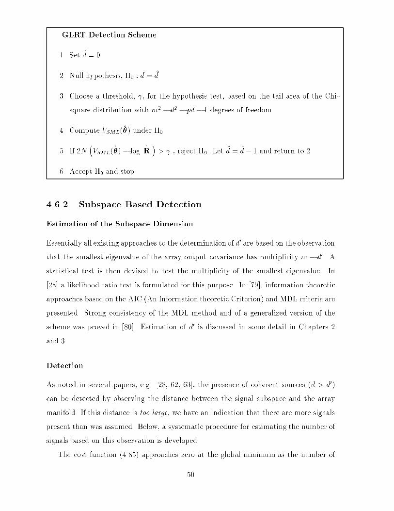
GLRT Detection Scheme

� Set $d �

�� Null hypothesis� H� � d $d�

� Choose a threshold� �� for the hypothesis test� based on the tail area of the Chi�

square distribution with m� � d� � pd � degrees of freedom�

�� Compute VSML�$�� under H��

�� If �N�VSML�$��� log

��� $R��� � � � reject H�� Let $d $d! and return to �

�� Accept H� and stop�

���� Subspace Based Detection

Estimation of the Subspace Dimension

Essentially all existing approaches to the determination of d� are based on the observation

that the smallest eigenvalue of the array output covariance has multiplicity m � d�� A

statistical test is then devised to test the multiplicity of the smallest eigenvalue� In

���� a likelihood ratio test is formulated for this purpose� In ����� information theoretic

approaches based on the AIC �An Information theoretic Criterion� and MDL criteria are

presented� Strong consistency of the MDL method and of a generalized version of the

scheme was proved in ����� Estimation of d� is discussed in some detail in Chapters �

and �

Detection

As noted in several papers� e�g� ���� ��� � �� the presence of coherent sources �d � d��

can be detected by observing the distance between the signal subspace and the array

manifold� If this distance is too large� we have an indication that there are more signals

present than was assumed� Below� a systematic procedure for estimating the number of

signals based on this observation is developed�

The cost function ������ approaches zero at the global minimum as the number of

��

data becomes large� provided that the correct dimensions� d and d� are chosen� If d is

chosen too small the cost increases� A statistical test is necessary to decide when the

cost function is close enough to zero for concluding that the choice of d is correct� The

test can be formulated as chosing between

H� � There are d signals

H� � There are more than d signals

Clearly� H� should be accepted when the value of the WSF criterion function is small�

The following result provides the necessary basis for appropriately setting the threshold�

Theorem ��� Under H�� the normalized WSF cost function

�N

$�VWSF ���

�N

$�TrfP�

A���$Es$Wopt

$EHs g � ������

evaluated at �� is asymptotically Chi�squared distributed with �d��m� d� degrees of free�

dom� When the criterion is evaluated at $�� the asymptotic distribution is still Chi�square�

but with �d��m � d� � pd degrees of freedom� Here $� refers to any consistent estimate

of the noise variance�

Proof See Appendix B� �

An algorithm for detection� based on Theorem ���� is outlined below� The signal subspace

dimension or an estimate thereof is assumed available�

�

WSF Detection Scheme

� Set $d d��

�� Null hypothesis� H� � d $d�

� Choose a threshold� �� for the hypothesis test� based on the tail area of the Chi�

square distribution with �d��m� d�� pd degrees of freedom�

�� Compute VWSF �$�� under H��

�� If �N���VWSF �$�� � � � reject H�� Let $d $d! � and return to �

�� Accept H� and stop�

By appropriately chosing the threshold� �� the user can determine the �asymptotic�

error�rate of the test� According to Theorem ���� the probability of rejecting H� when it

is true� is equal to the tail area of the corresponding ���distribution� Consequently� the

above technique does not yield a consistent estimate of d� To guarantee correct detection

for su�ciently large sample sizes� the threshold must be allowed to depend on N � In ����

it is shown that if � ��N� is chosen to satisfy

limN��

��N�

N � ���� �

limN��

��N�

log logN � ������

the estimate of the number of signals is strongly consistent� In practice� consistent

detection may be of little interest� since only a xed number of snapshots are available�

Note that the WSF criterion does not require a consistent estimate of the signal

subspace dimension d� to ensure a consistent detection and estimation procedure� This

is seen by letting d� m� �step above is then replaced by $d � and estimating $�

by the smallest eigenvalue of the sample covariance matrix� The smallest eigenvalue is

a consistent estimate of the noise variance� and asymptotically $Wopt �$�s � $�I�� $���s

provides a rank d� matrix with the correct weights� However� for obtaining e�cient

estimates it is crucial that the signal subspace dimension is not underestimated� see also

�����

��

For small sample sizes the situation is rather di�erent� When the signal waveforms

are highly correlated but not coherent� the signal covariance is nearly rank decient� The

small sample behavior of the detection�estimation scheme can then often be improved

by underestimating d�� For su�ciently high signal correlation� this will in fact be done

by any of the well known tests of the multiplicity of the smallest eigenvalue� see e�g�

���� ����

�

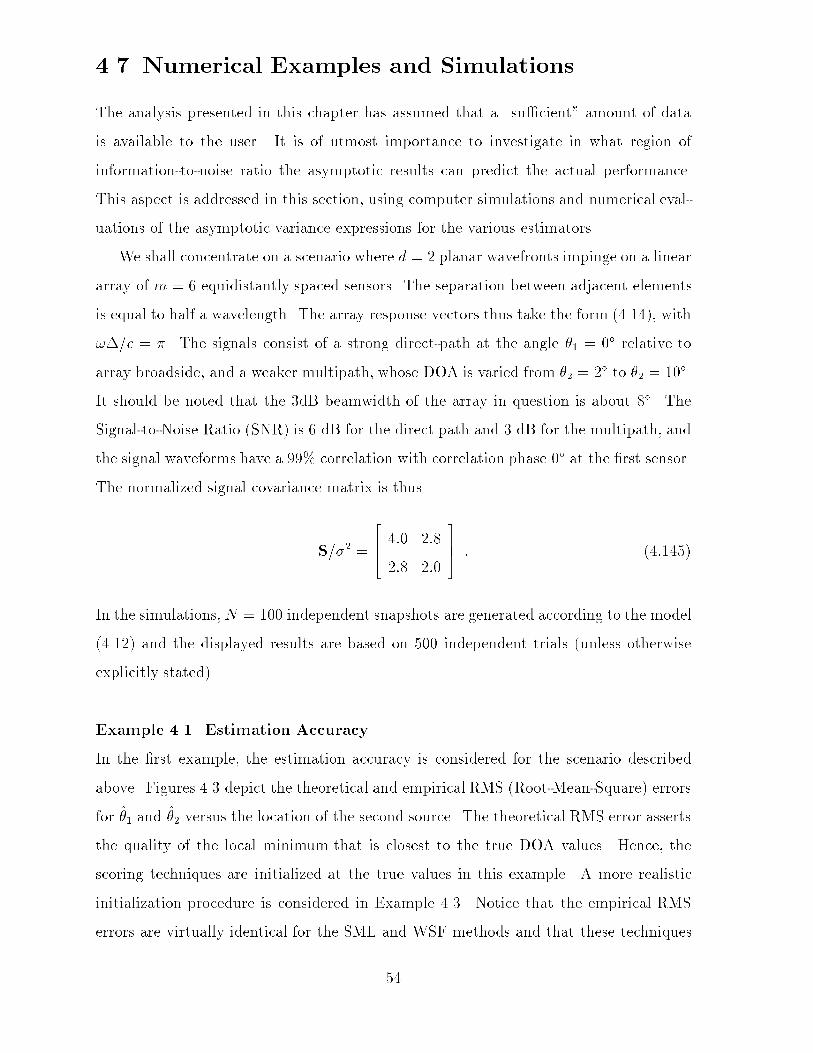
��� Numerical Examples and Simulations

The analysis presented in this chapter has assumed that a �su�cient� amount of data

is available to the user� It is of utmost importance to investigate in what region of

information�to�noise ratio the asymptotic results can predict the actual performance�

This aspect is addressed in this section� using computer simulations and numerical eval�

uations of the asymptotic variance expressions for the various estimators�

We shall concentrate on a scenario where d � planar wavefronts impinge on a linear

array of m � equidistantly spaced sensors� The separation between adjacent elements

is equal to half a wavelength� The array response vectors thus take the form ������ with

�"�c �� The signals consist of a strong direct�path at the angle �� �� relative to

array broadside� and a weaker multipath� whose DOA is varied from �� �� to �� �

��

It should be noted that the dB beamwidth of the array in question is about ��� The

Signal�to�Noise Ratio �SNR� is � dB for the direct path and dB for the multipath� and

the signal waveforms have a ��% correlation with correlation phase �� at the rst sensor�

The normalized signal covariance matrix is thus

S��

��� ��� ���

��� ���

��� � ������

In the simulations�N �� independent snapshots are generated according to the model

����� and the displayed results are based on ��� independent trials �unless otherwise

explicitly stated��

Example ��� Estimation Accuracy

In the rst example� the estimation accuracy is considered for the scenario described

above� Figures �� depict the theoretical and empirical RMS �Root�Mean�Square� errors

for $�� and $�� versus the location of the second source� The theoretical RMS error asserts

the quality of the local minimum that is closest to the true DOA values� Hence� the

scoring techniques are initialized at the true values in this example� A more realistic

initialization procedure is considered in Example �� � Notice that the empirical RMS

errors are virtually identical for the SML and WSF methods and that these techniques

��

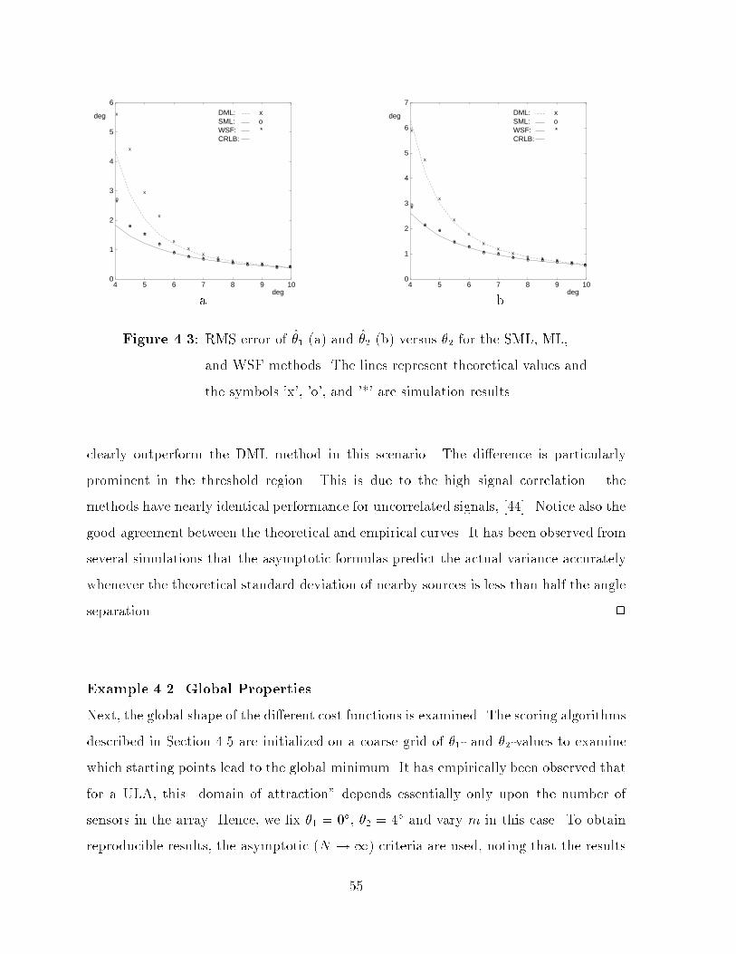
0

1

2

3

4

5

6

4 5 6 7 8 9 10

x

x

x

x

x

xx

xx x x

x x

o

o

o

o

oo o o o o o o o

*

**

** * * * * * * * *

deg

deg

DML: xSML: oWSF: *CRLB:

0

1

2

3

4

5

6

7

4 5 6 7 8 9 10

x

x

x

x

x

xx

xx x x x x

o

oo

oo

o oo o o o o o

*

**

**

* * * * * * * *

deg

deg

DML: xSML: oWSF: *CRLB:

a b

Figure ��� RMS error of $�� �a� and $�� �b� versus �� for the SML� ML�

and WSF methods� The lines represent theoretical values and

the symbols �x�� �o�� and �&� are simulation results�

clearly outperform the DML method in this scenario� The di�erence is particularly

prominent in the threshold region� This is due to the high signal correlation � the

methods have nearly identical performance for uncorrelated signals� ����� Notice also the

good agreement between the theoretical and empirical curves� It has been observed from

several simulations that the asymptotic formulas predict the actual variance accurately

whenever the theoretical standard deviation of nearby sources is less than half the angle

separation� �

Example ��� Global Properties

Next� the global shape of the di�erent cost functions is examined� The scoring algorithms

described in Section ��� are initialized on a coarse grid of ��� and ���values to examine

which starting points lead to the global minimum� It has empirically been observed that

for a ULA� this �domain of attraction� depends essentially only upon the number of

sensors in the array� Hence� we x �� ��� �� �� and vary m in this case� To obtain

reproducible results� the asymptotic �N � � criteria are used� noting that the results

��

will be similar for all values of N above a certain threshold� Figure ��� shows the results

form � andm �� whereas the cases ofm � andm � are presented in Figure ����

The region of attraction is identied as the �completely lled� area surrounding the

global minimum� From the gures we see that the SML and WSF methods have similar

regions of attraction in the scenarios in question and the region for the DML method is

smaller in all cases� It is also interesting to observe that for the WSF algorithm� there

are a large number of starting points further away from the minimum that also lead to

global convergence� However� the number of such points is reduced as m is increased� It

is quite clear from this example that proper initialization of the search methods becomes

more crucial with increasing array aperture� In ����� this e�ect is studied in some detail

for the related problem of estimating the frequencies of superimposed sinusoids� The

asymptotic �for large m� radius of the domain of attraction for the DML algorithm is

found to be inversely proportional to m� This is in good agreement with the empirical

results presented in this example� This observation suggests that for large m� the initial

estimates should have a variance of order o��m�� �for a ULA� to guarantee global

convergence of the search algorithm� Simulation results presented in ���� �see also below�

indicate that this is indeed the case for the AP initialization scheme� �

Example �� Initialization and Number of Iterations

In this example� the scoring techniques for minimizing the di�erent cost functions are

studied in some more detail� The alternating projection initialization scheme suggested

in ���� is used for initializing the scoring methods described in Section ���� The original

version is used for the SML and DML methods� whereas the same schemewith $R replaced

by $Es$Wopt

$EHs is used for the WSF technique� The overall performance is assessed by

displaying the probability of reaching the global minimum �Figure ���a� and the average

number of iterations necessary to fulll the stopping condition �Figure ���b� versus ���

The iterations terminated successfully when jH��V �j ���� in the vast majority of thetrials �more than ��% for �� ��� In a small number of trials in the threshold region�the maximum number of iterations �set to �� was reached or the search terminated at

a point were no improvement could be found along the scoring direction ��k �������

��

From Figure ���a� it is clear that the AP initialization scheme performs excellent for the

WSF method � the global minimum was reached in all trials� However� a large number

of iterations is necessary in the di�cult cases where the angle separation is less than

�� The AP initialization performs satisfactory also for the DML method and somewhat

worse� but still acceptable for the SML technique� Recall that the RMS error for $�� is

more than half the angle separation when �� ����� Notice also that for �� � ��� the

WSF�scoring technique converges in a smaller number of iterations than the DML and

SML scoring methods� Still� the DML�scoring technique performs signicantly better

than the modied Gauss�Newton technique suggested in ����� �

Example ��� Detection Performance

In the nal example� we compare the performance of the various detection procedures

outlined in Section ���� The scenario is the same as in the previous examples� The

estimates are calculated as in Example �� � Figure ��� displays the probability of correct

detection versus the location of the second source for the di�erent detection schemes�

The detection results from the MDLC method of ���� are included for comparison� This

scheme is based on the DML cost function and relies on the DML estimates� The WSF

detection scheme requires information of the signal subspace dimension� The MDL test

of ���� is used for this purpose� which results in the value d� in all trials� As seen

from Figure ���� the WSF detection scheme has a slightly lower threshold than the GLRT

based technique� whereas the MDLC criterion performs clearly worse� Note that as ��

increases� the detection probabilities for the WSF and GLR tests approach the value

preset by the threshold� Another important observation is that the threshold value of

the angle separation for the WSF and GLRT detection schemes �about �� for WSF and

���� for GLRT� is lower than the value at which reliable estimates is obtained �e�g�� when

the standard deviation of both angle estimates is lower than half the angle separation�� cf�

Figure �� b� On the other hand� the value at which the global minimum can be reached

using the AP initialization scheme is still lower for the WSF algorithm �less than ����

whereas it is similar to the detection threshold for the SML method and the GLR test�

cf� Figure ���a� One may suspect that the initialization procedure indeed is the limiting

��

factor for the GLR test� This is� however� not the case� since for �� � ��� essentially allerrors are due to underestimation of d� so the detection performance cannot be improved

upon by using a more e�cient initialization procedure� In summary� this observation

suggests that the estimation accuracy is indeed the limiting factor for both the WSF and

the SML methods if the proposed schemes for calculating the estimates and determining

the number of sources are used� However� the estimation accuracy is the best possible

in terms of estimation error variance� Of course� no general conclusions can be drawn

from the rather limited scenario presented in this study� but similar observations have

been made also in other cases� see e�g�� ����� �

��

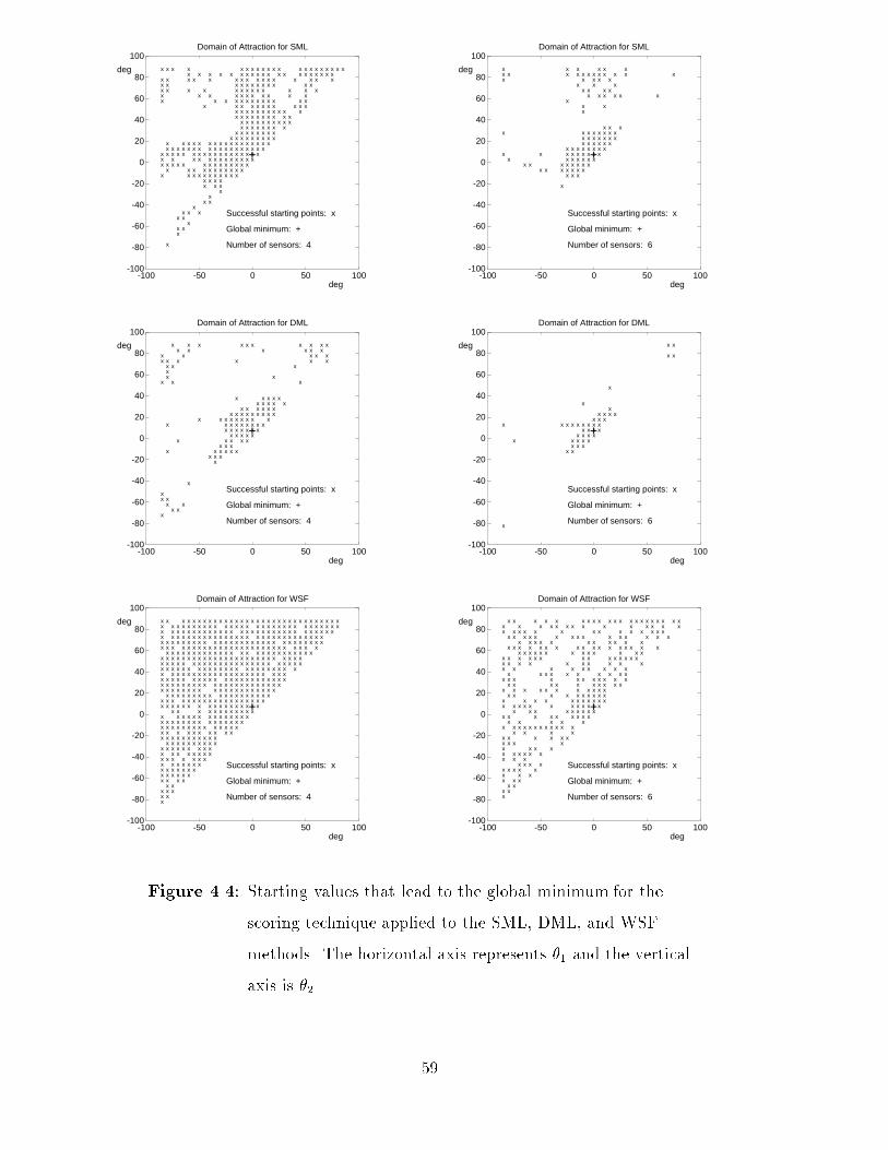
-100

-80

-60

-40

-20

0

20

40

60

80

100

-100 -50 0 50 100

x

xxx

xxxxx

x

x

xx

xxx

xxx

x

xxxx

x

xx

x

x

xx

x

xx

x

xxx

x

x

xx

xx

x

xxx

x

xx

xxxx

x

x

x

xxxx

x

x

x

xxxxx

x

x

x

xx

xxxxxxxx

x

xx

xxxxxxxxx

x

xxxxxxxxxx

x

xxxxxxx

x

xxxxxxxx

x

xxxxxxxxx

xxxxxxxx

xxxxxxxxxxxxxxxxxxxx

xxxxxxxxxxx

xxxxxxx

xxxxxxxxxxxxxxx

xx

xxxxxxxxxxx

xxxxx

xxxxxxxxxxxxxxxx

xxxxxxxxxx

xxxx

xxxxxxxx

xx

x

x

x

xx

xxxx

x

xx

xx

x

x

xxx

xx

xxxxx

xx

xxxx

x

xxx

xx

xx

xxx x x

+

Domain of Attraction for SML

deg

deg

Successful starting points: x

Global minimum: +

Number of sensors: 4

-100

-80

-60

-40

-20

0

20

40

60

80

100

-100 -50 0 50 100

x

x

xxx

x

x

x xx

x

x

x

xx

xxxxxx

x

xx

xxxxxx

xxxxxx

x

xx

xxxxxxxx

xx

x

xx

xxxxxxx

xx

x

xxxxxx

xxx

xxxxx

x

xxx

xxxxx

x

xx

xx

xxxx

x

x

xx

x

x

x

x

x

xx

x

x

+

Domain of Attraction for SML

deg

deg

Successful starting points: x

Global minimum: +

Number of sensors: 6

-100

-80

-60

-40

-20

0

20

40

60

80

100

-100 -50 0 50 100

x

xx

x

xx

xx

x

x

xxxx

x

x

x

x

x

x

x

x

x

x

x

xx

x

x

xxxx

xxx

x

xxx

xxx

xxxxxxxx

x

xxxxx

x

x

xxxxxxx

x

xxxxxxx

x

xxxxx

x

xx

xxx

x

xxxx

x

xxxxx

xxxx

x

xx

x

x

xx

xxxx

xxx

xx

x

+

Domain of Attraction for DML

deg

deg

Successful starting points: x

Global minimum: +

Number of sensors: 4

-100

-80

-60

-40

-20

0

20

40

60

80

100

-100 -50 0 50 100

x

x

x

x

x

x

xxx

x

xxx

x

xxxxx

x

xxxx

xxxx

xxxx

xx x

x

x

x

x

x

x

x

+

Domain of Attraction for DML

deg

deg

Successful starting points: x

Global minimum: +

Number of sensors: 6

-100

-80

-60

-40

-20

0

20

40

60

80

100

-100 -50 0 50 100

xxx

xxxxxxx

xxxxx

xx

xxxxxxx

xxxxxx

xxxxxx

x

xxxxxx

xxxxxx

xxxxxx

x

xx

xxxxxxxx

xx

xxxxxxxxxxxxxxxxx

xxxx

xxxxxxxxxx

xxxxxxxxx

xxxx

xxxxx

xxx

xxx

xxxxxxxxxxxxxxxxx

xxx

xxxxxxxx

xxxxx

xx

xxxxxxxx

xxxx

xxxxxx

xxxxxx

xxxxxxxxx

xxxxxxxxxxxxxxxxxxxxxxxxxxxx

xxxxx

x

xx

xxxxxxxxxxxxx

xxxxx

xxxxxx

xxxxxxx

xxxx

xxxxxxxxx

xxxxxxxxxxxxxx

xxxxxxxxx

xxxxxxxxx

x

xxxxxxxxxxxxxxxxxxxxxx

xxxxxxxxxxxxxxxxxxxxxx

xxxxxxxxxxxxxx

xxx

xx

xxxxxxxxxx

xxxxxxxxx

xxxxxxxxxxxxxxxxxxx

xxxxxxxxxxx

xx

x

x

xxxxxxxxxxxxxxxxx

xxxxxxxxxxxxxxxx

xxxx

xxxxxxxxxx

xxxxx

xxxxxxxx

xxxxx

xx

xxxx

xxxxxxxxxxxx

xxx

xxxxx

xxxxxxxxxx

xxxxxx

x

xxxxxxx

x

xxxxx

xxxxxx

xxxxx

xxx

xxx

xx

+

Domain of Attraction for WSF

deg

deg

Successful starting points: x

Global minimum: +

Number of sensors: 4

-100

-80

-60

-40

-20

0

20

40

60

80

100

-100 -50 0 50 100

xx

xxx

xxxxx

x

x

xx

x

x

xxx

xx

xx

x

xx

xx

x

xxx

xx

x

x

x

xx

x

xx

x

xx

xx

xxxx

x

x

xx

x

xxxx

x

xx

x

xxxxx

xx

xxx

xx

xx

x

x

xx

x

x

xx

x

xx

xxxxxx

x

x

x

x

xx

x

xx

xxx

x

x

x

x

x

x

xxxx

x

x

x

x

x

xx

x

x

xxxxx

x

x

xxxx

x

x

x

x

xx

x

x

xx

xx

xx

x

x

x

x

x

x

x

xx

xxxx

x

x

x

x

xxxxxxxxx

x

x

xxxxxx

x

xxxxx

x

xx

xxxxxx

xxxx

x

x

xxxxxxx

xxx

x

x

xxxxxxx

x

x

x

xxxxx

x

x

x

xx

xxx

x

xx

x

x

x

x

x

x

xxxx

xx

x

xxx

x

xxx

x

x

xxx

xx

x

x

xxx

x

x

x

xx

xxx

x

xx

x

xxx

x

xxx

+

Domain of Attraction for WSF

deg

deg

Successful starting points: x

Global minimum: +

Number of sensors: 6

Figure ���� Starting values that lead to the global minimum for the

scoring technique applied to the SML� DML� and WSF

methods� The horizontal axis represents �� and the vertical

axis is ���

��

-100

-80

-60

-40

-20

0

20

40

60

80

100

-100 -50 0 50 100

xx

xxxxx

xxxxx

x

xxxxxx

xx

x

xxxxx

x

xx

xxxx

x

x

xxxx

x

xx

xx

xx x

+

Domain of Attraction for SML

deg

deg

Successful starting points: x

Global minimum: +

Number of sensors: 8

-100

-80

-60

-40

-20

0

20

40

60

80

100

-100 -50 0 50 100

xx

xxxx

xxx

xxxxx

xx

xxxx

x

xxx

xxx

x

+

Domain of Attraction for SML

deg

deg

Successful starting points: x

Global minimum: +

Number of sensors: 10

-100

-80

-60

-40

-20

0

20

40

60

80

100

-100 -50 0 50 100

x

x x xx x

xx

xxx

xxx

xxx x

xxx

x

+

Domain of Attraction for DML

deg

deg

Successful starting points: x

Global minimum: +

Number of sensors: 8

-100

-80

-60

-40

-20

0

20

40

60

80

100

-100 -50 0 50 100

x

x

xx

x

x

xxx

xxx

x

xxxxx

xx

xx

xxx

+

Domain of Attraction for DML

deg

deg

Successful starting points: x

Global minimum: +

Number of sensors: 10

-100

-80

-60

-40

-20

0

20

40

60

80

100

-100 -50 0 50 100

x

x

x

x

x

x

x

x

x

x

x

x

x

x

x

x

x

x

xx

x

x

x

x

xx

x

x

xxx

x

xx

x

x

xx

xx

x

x

x

x

x

x

xxxxx

x

xx

x

x

x

xxx

x

x

x

xxx

x

x

xx

x

x

x

xx

xx

x

xx

x

xx

xx

x

xx

x

xxxx

x

x

x

xxx

xxxxx

x

xx

x

xxxxx

x

x

x

xxx

x

x

xx

xxx

x

x

x

x

x

x

x

x

x

x

x

x

xx

xx

x

xxxx

xx

xx

x

+

Domain of Attraction for WSF

deg

deg

Successful starting points: x

Global minimum: +

Number of sensors: 8

-100

-80

-60

-40

-20

0

20

40

60

80

100

-100 -50 0 50 100

x

xx

x

x

x

x

x

xx

x

x

xxx

x

x

x

x

xx

x

x

x

x

x

xx

x

x

x

x

x

x

xx

x

x

x

x

x

x

x

x

x

x

x

x

x

xx

x

x

xx

x

x

x

x

xxxx

xxx

xxxxx

x

xx

xxx

xx

x

xx

x

x

x

x

x

x

xx

x

x

x x

x

x

x

x

x

x

x

x

x

x

xx

x

x

+

Domain of Attraction for WSF

deg

deg

Successful starting points: x

Global minimum: +

Number of sensors: 10

Figure �� � Starting values that lead to the global minimum for the

scoring technique applied to the SML� DML� and WSF

methods� The horizontal axis represents �� and the vertical

axis is ���

��

0.5

0.6

0.7

0.8

0.9

1

1.1

2 3 4 5 6 7 8 9 10

Prob

deg

WSF:DML:SML:

1

2

3

4

5

6

7

8

9

10

11

2 3 4 5 6 7 8 9 10

# iter

deg

WSF:SML:DML:

a b

Figure ���� Probability of global convergence �a� and average number of

iterations �b� versus �� for the SML� DML� and WSF methods�

0

0.1

0.2

0.3

0.4

0.5

0.6

0.7

0.8

0.9

1

2 3 4 5 6 7 8 9 10

Prob

deg

WSF, 95% :GLRT, 95% :MDLC :

0

0.1

0.2

0.3

0.4

0.5

0.6

0.7

0.8

0.9

1

2 3 4 5 6 7 8 9 10

Prob

deg

WSF, 99% :GLRT, 99% :MDLC :

a b

Figure ���� Probability of correct detection using ��% �a� and ��% �b�

condence levels versus �� for the GLRT and WSF detection

schemes� The results for the MDLC technique is the same in

both plots� since it requires no threshold setting�

�

��� Conclusions

This chapter presents exact and large sample realizations of ML estimation techniques

for signal parameter estimation from array data� Two di�erent signal models �determin�

istic vs� stochastic� are considered and the ML estimator is formulated for each model�

The asymptotic properties of these methods are examined and related to the correspond�

ing Cram�er�Rao lower bounds� The stochastic ML �SML� method is found to provide

more accurate estimates than the deterministic ML �DML� technique� independent of

the actual emitter signal waveforms� Under the Gaussian signal assumption� the SML

method is asymptotically e�cient� i�e�� the estimation error attains the CRLB�

Two classes of multidimensional subspace or eigenstructure techniques are presented�

the noise and signal subspace formulations� The relation between the these is established

by comparing their asymptotic distributions� The subspace methods that are asymp�

totically identical to the ML techniques are identied� In the case of coherent signals

�specular multipath�� only the signal subspace version can yield optimal �SML� per�

formance� This optimal signal subspace method is termed WSF �Weighted Subspace

Fitting��

All methods considered herein require a multidimensional search to nd the param�

eter estimates� Newton�type descent algorithms for calculating the ML and signal sub�

space estimates are presented� and their implementation and initialization is discussed�

The Newton�type algorithm for the signal subspace formulation requires O�md�� �ops

per iteration� whereas both ML implementations cost O�m�d�� Consequently� the sub�

space technique o�ers a computational advantage when the number of emitters �d� is

less than the number of sensors �m��

A generalized likelihood ratio test �GLRT� for determining the number of emitters

is derived� as well as a detection scheme based on the WSF criterion� The methods are

similar in structure� and require a threshold which sets the �asymptotic� probability of

detection�

Numerical examples and simulations are presented� comparing the various detection

and estimation algorithms� Examples studying empirical vs� theoretical estimation

accuracy� global convergence properties� average number of iterations� and detection

��

performance are included� The performance of the WSF and SML�GLRT techniques is

found to be limited only by the estimation accuracy� In other words� global convergence

and correct detection is obtained with high probability whenever accurate parameter

estimation is possible� In these cases� the estimation error variance is found to be in good

agreement with the theoretical variance� based on the asymptotic covariance matrix�

�

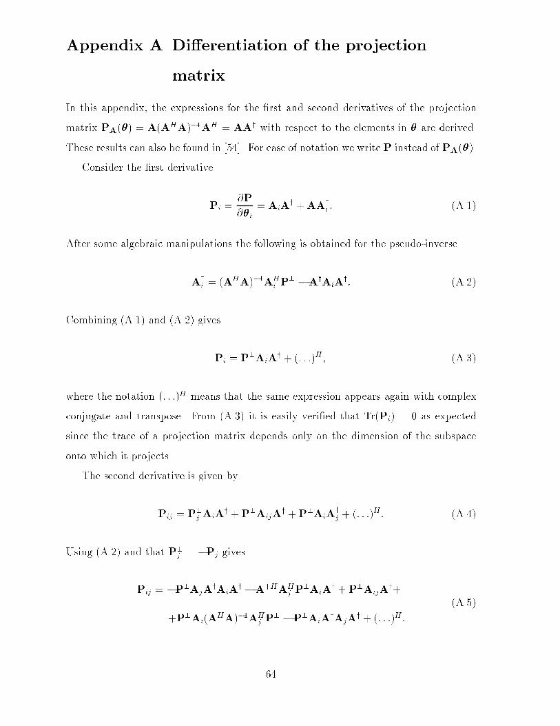
Appendix A Di erentiation of the projection

matrix

In this appendix� the expressions for the rst and second derivatives of the projection

matrix PA��� A�AHA���AH AAy with respect to the elements in � are derived�

These results can also be found in ����� For ease of notation we write P instead of PA����

Consider the rst derivative

Pi �P

��i AiA

y !AAyi � �A��

After some algebraic manipulations the following is obtained for the pseudo�inverse

Ayi �A

HA���AHi P

� �AyAiAy� �A���

Combining �A�� and �A��� gives

Pi P�AiAy ! �� � ��H � �A� �

where the notation �� � ��H means that the same expression appears again with complex

conjugate and transpose� From �A� � it is easily veried that Tr�Pi� � as expected

since the trace of a projection matrix depends only on the dimension of the subspace

onto which it projects�

The second derivative is given by

Pij P�j AiA

y !P�AijAy !P�AiA

yj ! �� � ��

H � �A���

Using �A��� and that P�j �Pj gives

Pij �P�AjAyAiA

y �A�HAHj P

�AiAy !P�AijA

y!

!P�Ai�AHA���AHj P

� �P�AiAyAjA

y ! �� � ��H�

�A���

��

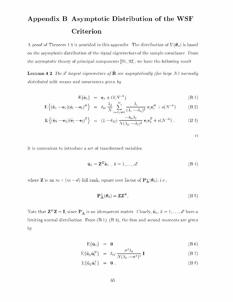
Appendix B Asymptotic Distribution of the WSF

Criterion

A proof of Theorem ��� is provided in this appendix� The distribution of V ���� is based

on the asymptotic distribution of the signal eigenvectors of the sample covariance� From

the asymptotic theory of principal components ��� ���� we have the following result�

Lemma ��� The d� largest eigenvectors of $R are asymptotically �for large N� normally

distributed with means and covariances given by

Ef$ekg ek !O�N��� �B��

En�$ek � ek��$el � el�

Ho kl

�kN

mXi���i�k

�i��i � �k��

eieHi ! o�N��� �B���

En�$ek � ek��$el � el�

To �� kl�

��k�lN��k � �l��

eleTk ! o�N��� � �B� �

�

It is convenient to introduce a set of transformed variables

$uk ZH$ek � k � � � � � d� �B���

where Z is an m �m� d� full rank� square root factor of P�A����� i�e��

P�A���� ZZH � �B���

Note that ZHZ I� since P�Ais an idempotent matrix� Clearly� $uk� k � � � � � d� have a

limiting normal distribution� From �B����B� �� the rst and second moments are given

by

Ef$ukg � �B���

Ef$uk$uHl g kl��k

N��k � ���I �B���

Ef$uk$uTl g � � �B���

��

From ������� we can rewrite the normalized WSF cost function as

�N

$�VWSF ����

�N

$�TrfZZH $Es

$Wopt$EHs g

�N

$�

d�Xk��

$wk$uHk $uk

�N

$�$uH $u

�N

$���uT �u ! #uT #u� � �B���

where $wk �$�k � $����$�k� $u hp$w�$uT� � � �

p$wd� $uTd�

iT� �u Re�$u�� and #u Im�$u��

Since $u is of order Op�N����� for large N � we can replace the consistent estimates of

� and �k above with the true quantities without changing the asymptotic properties�

The assertion on the asymptotic distribution of VWSF ���� then follows from the fact

that �B��� is a sum of �d��m � d� squared random variables that are asymptotically

independent and N�����

To determine the distribution of the cost function evaluated at the parameter esti�

mate� consider the Taylor series expansions

V �$�� V ���� ! V �T ����#� !

�#�TV ������#� ! o�j#�j�� �B���

V ��$�� � V ����� ! V ������#� ! o�j#�j� �B��

�where the subscript has been dropped from VWSF ��� for notational convenience�� Here�

#� denotes the estimation error� #� $� � ��� The regularity assumptions on the array

response vectors guarantee that V ������ converges �w�p�� as N � � The limitingHessian� denoted H� is assumed to be non�singular� Equations �B�����B�� can be

written

V �$�� V ���� ! V �T ����#� !

�#�TH#� ! o�j#�j��� �B���

V ��$�� � V ����� !H#� ! o�j#�j� � �B� �

The �in�probability� rate of convergence of the estimation error is Op�N������ Thus�

inserting �B� � into �B��� yields

V �$�� � V ����� V �T ����H��V ����� !

�V �T ����H

��V �����

��

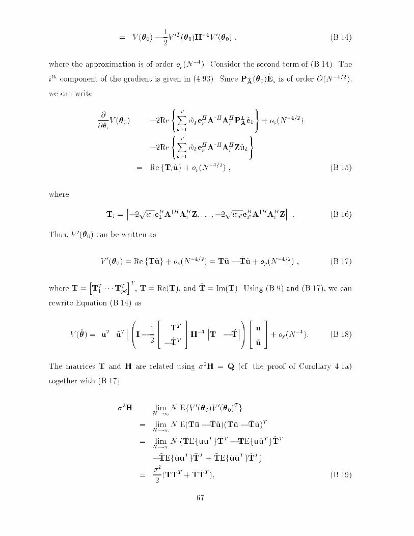
V ����� �V �T ����H

��V ����� � �B���

where the approximation is of order op�N���� Consider the second term of �B���� The

ith component of the gradient is given in ���� �� Since P�A����$Es is of order O�N

������

we can write

�

��iV ���� ��Re

���d�Xk��

$wkeHk A

yHAHi P

�A$ek

���! op�N�����

��Re���

d�Xk��

$wkeHk A

yHAHi Z$uk

��� Re fTi$ug! op�N

����� � �B���

where

Ti h��pw�e

H� A

yHAHi Z� � � � ���

pwd�e

Hd�A

yHAHi Z

i� �B���

Thus� V ����� can be written as

V ����� Re fT$ug! op�N����� �T�u� #T#u! op�N

����� � �B���

where T hTT

� � � �TTpd

iT� �T Re�T�� and #T Im�T�� Using �B��� and �B���� we can

rewrite Equation �B��� as

V �$�� h�uT #uT

i�B�I� �

��� �TT

�#TT

���H��h�T � #T

i�CA��� �u#u

���! op�N���� �B���

The matrices T and H are related using �H Q �cf� the proof of Corollary ��a�

together with �B���

�H limN��

N EfV �����V�����

Tg lim

N��N E��T�u� #T#u�� �T�u � #T#u�T

limN��

N � �TEf�u�uTg�TT � �TEf�u#uTg#TT

�#TEf#u�uTg�TT ! #TEf#u#uTg#TT �

�

�� �T�TT ! #T #TT �� �B���

��

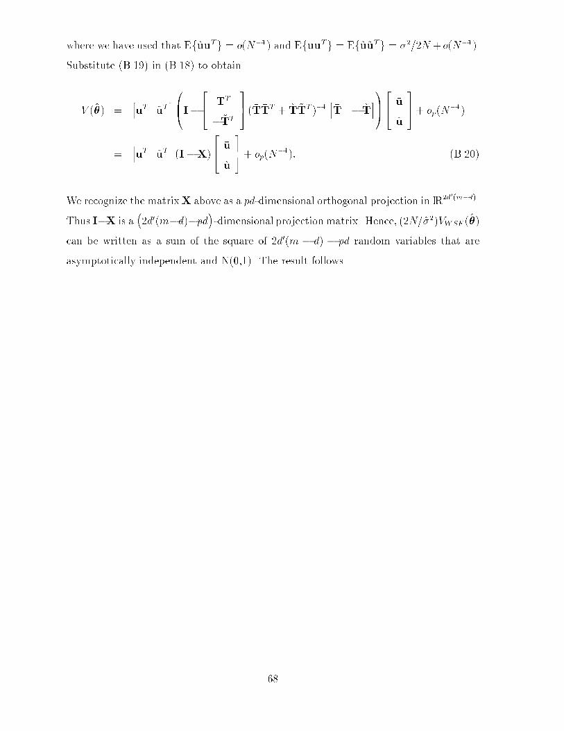
where we have used that Ef#u�uTg o�N��� and Ef�u�uTg Ef#u#uTg ���N ! o�N����

Substitute �B��� in �B��� to obtain

V �$�� h�uT #uT

i�B�I���� �TT

�#TT

��� � �T�TT ! #T#TT ���h�T � #T

i�CA��� �u#u

���! op�N���

h�uT #uT

i�I�X�

��� �u#u

���! op�N���� �B����

We recognize the matrixX above as a pd�dimensional orthogonal projection in IR�d��m�d��

Thus I�X is a��d��m�d��pd

�dimensional projection matrix� Hence� ��N�$��VWSF �$��

can be written as a sum of the square of �d��m � d� � pd random variables that are

asymptotically independent and N����� The result follows�

��

References

�� S� P� Applebaum� �Adaptive Arrays�� Technical Report SPL TR ���� Syracuse

University Research Corporation� August ����

��� B� Widrow� P�E� Mantey� L�J� Gri�ths� and B�B� Goode� �Adaptive Antenna Sys�

tems�� Proc� IEEE� ��� ����� Dec� ����

� � F�C� Schweppe� �Sensor Array Data Processing for Multiple Signal Sources�� IEEE

Trans� on IT� IT������� ��� ����

��� V�H� MacDonald and P�M� Schultheiss� �Optimum Passive Bearing Estimation in a

Spatially Incoherent Noise Environment�� J� Acoust� Soc� Am�� ����� ��� � ����

��� J� Capon� �High Resolution Frequency Wave Number Spectrum Analysis�� Proc�

IEEE� ��������� ����

��� R�A� Monzingo and T�W� Miller� Introduction to Adaptive Arrays� Wiley� ����

��� S� Haykin� editor� Array Signal Processing� Prentice�Hall� Englewood Cli�s� NJ�

����

��� B�D� Van Veen and K�M� Buckley� �Beamforming� A Versatile Approach to Spatial

Filtering�� IEEE ASSP Magazine� pages ����� April ����

��� J� P� Burg� �Maximum Entropy Spectral Analysis�� In Proceedings of the �th

Annual International SEG Meeting� Oklahoma City� OK�� ����

��� D�W� Tufts and R� Kumaresan� �Estimation of Frequencies of Multiple Sinu�

soids� Making Linear Prediction Perform Like Maximum Likelihood�� Proc� IEEE�

����������� Sept� ����

�� R� Kumaresan and D�W� Tufts� �Estimating the Angles of Arrival of Multiple Plane

Waves�� IEEE Trans� Aerosp� Electron� Syst�� AES��� �� �� Jan� �� �

��� R�O� Schmidt� �Multiple Emitter Location and Signal Parameter Estimation�� In

Proc� RADC Spectrum Estimation Workshop� pages �� ����� Rome� NY� ����

��

� � G� Bienvenu and L� Kopp� �Principle de la goniometrie passive adaptive�� In

Proc� ��eme Colloque GRESIT� pages ��������� Nice� France� ����

��� G� Bienvenu and L� Kopp� �Adaptivity to Background Noise Spatial Coherence for

High Resolution Passive Methods�� In Proc� IEEE ICASSP� pages ��� �� Denver�

CO�� ����

��� N�L� Owsley� �Data Adaptive Orthonormalization�� In Proc� ICASSP ��� pages

����� Tulsa� OK� ����

��� V�F� Pisarenko� �The retrieval of harmonics from a covariance function�� Geophys�

J� Roy� Astron� Soc�� � ��� ��� �� �

��� G� Bienvenu and L� Kopp� �Optimality of High Resolution Array Processing��

IEEE Trans� ASSP� ASSP��� ������ Oct� �� �

��� A� Paulraj� R� Roy� and T� Kailath� �A Subspace Rotation Approach to Signal

Parameter Estimation�� Proceedings of the IEEE� pages �������� July ����

��� S�Y� Kung� C�K� Lo� and R� Foka� �A Toeplitz Approximation Approach to Coher�

ent Source Direction Finding�� In Proc� ICASSP � � ����

���� S�J� Orfanidis� �A Reduced MUSICAlgorithm�� In Proc� IEEE ASSP rd Workshop

Spectrum Est� Modeling� pages ������ Boston� MA� Nov� ����

��� W� J� Bangs� Array Processing with Generalized Beamformers� PhD thesis� Yale

University� New Haven� CT� ���

���� M� Wax� Detection and Estimation of Superimposed Signals� PhD thesis� Stanford

Univ�� Stanford� CA� March ����

�� � J�F� B'ohme� �Estimation of Source Parameters By Maximum Likelihood and Non�

linear Regression�� In Proc� ICASSP �� pages �� ���� ��� ����

���� J�F� B'ohme� �Estimation of Spectral Parameters of Correlated Signals in Wave�

elds�� Signal Processing� ��� ��� �� ����

��

���� P� Stoica and A� Nehorai� �MUSIC� MaximumLikelihood and Cram�er�Rao Bound��

In Proc� ICASSP �� Conf� pages ���������� New York� April ����

���� B� Ottersten and L� Ljung� �Asymptotic Results for Sensor Array Processing�� In

Proc� ICASSP ��� pages ���������� Glasgow� Scotland� May ����

���� B� Ottersten and M� Viberg� �Analysis of Subspace Fitting Based Methods for Sen�

sor Array Processing�� In Proc� ICASSP ��� pages ��������� Glasgow� Scotland�

May ����

���� R� O� Schmidt� A Signal Subspace Approach to Multiple Emitter Location and

Spectral Estimation� PhD thesis� Stanford Univ�� Stanford� CA� Nov� ���

���� B� Ottersten� B� Wahlberg� M� Viberg� and T� Kailath� �Stochastic Maximum

Likelihood Estimation in Sensor Arrays by Weighted Subspace Fitting�� In Proc�

� rd Asilomar Conf� Sig�� Syst�� Comput�� pages ������ � Monterey� CA� Nov� ����

� �� P� Stoica and A� Nehorai� �MUSIC� MaximumLikelihood and Cram�er�Rao Bound��

IEEE Trans� ASSP� ASSP��������� May ����

� � H� Clergeot� S� Tressens� and A� Ouamri� �Performance of High Resolution Fre�

quencies Estimation Methods Compared to the Cram�er�Rao Bounds�� IEEE Trans�

ASSP� ������ ����� November ����

� �� P� Stoica and A� Nehorai� �Performance Study of Conditional and Unconditional

Direction�of�Arrival Estimation�� IEEE Trans� ASSP� ASSP���� ����� Octo�

ber ����

� � K� Sharman� T�S� Durrani� M� Wax� and T� Kailath� �Asymptotic Performance

of Eigenstructure Spectral Analysis Methods�� In Proc� ICASSP � Conf� pages

������������� San Diego� CA� March ����

� �� D�J� Je�ries and D�R� Farrier� �Asymptotic Results for Eigenvector Methods�� IEE

Proceedings F� �������������� June ����

�

� �� M� Kaveh and A� J� Barabell� �The Statistical Performance of the MUSIC and

the Minimum�Norm Algorithms in Resolving Plane Waves in Noise�� IEEE Trans�

ASSP� ASSP�� � �� April ����

� �� B� Porat and B� Friedlander� �Analysis of the Asymptotic Relative E�ciency of the

MUSIC Algorithm�� IEEE Trans� ASSP� ASSP��� ������ April ����

� �� B� D� Rao and K� V� S� Hari� Performance analysis of root�music� IEEE Trans�

ASSP� ASSP������ ������ Dec� ����

� �� B� D� Rao and K� V� S� Hari� Performance analysis of ESPRIT and TAM in de�

termining the direction of arrival of plane waves in noise� IEEE Trans� ASSP�

ASSP������������� Dec� ����

� �� P� Stoica and A� Nehorai� �MUSIC� Maximum Likelihood and Cram�er�Rao Bound�

Further Results and Comparisons�� IEEE Trans� ASSP� ASSP���������� De�

cember ����

���� P� Stoica and A� Nehorai� �Performance Comparison of Subspace Rotation and

MUSIC Methods for Direction Estimation�� IEEE Trans� ASSP� Feb� ���

��� P� Stoica and K� Sharman� �A Novel Eigenanalysis Method for Direction Estima�

tion�� Proc� IEE� F������ Feb ����

���� P� Stoica and K� Sharman� �Maximum Likelihood Methods for Direction�of�Arrival

Estimation�� IEEE Trans� ASSP� ASSP�� ��� � July ����

�� � D� Starer� Algorithms for Polynomial�Based Signal Processing� PhD thesis� Yale

University� New Haven� CT� May ����

���� M� Viberg and B� Ottersten� �Sensor Array Processing Based on Subspace Fitting��

IEEE Trans� ASSP� ASSP�� May ���

���� B� Ottersten� M� Viberg� and T� Kailath� �Performance Analysis of the Total Least

Squares ESPRIT Algorithm�� IEEE Trans� on ASSP� ASSP�� May ���

��

���� Y� Bresler� �Maximum Likelihood Estimation of Linearly Structured Covariance

with Application to Antenna Array Processing�� In Proc� th ASSP Workshop on

Spectrum Estimation and Modeling� pages ������ Minneapolis� MN� Aug� ����

���� B� Ottersten� R� Roy� and T� Kailath� �Signal Waveform Estimation in Sensor Array

Processing�� In Proc� � rd Asilomar Conf� Sig�� Syst�� Comput�� Nov� ����

���� M� Wax and I� Ziskind� �On Unique Localization of Multiple Sources by Passive

Sensor Arrays�� IEEE Trans� on ASSP� ASSP������������� July ����

���� A� Nehorai� D� Starer� and P� Stoica� �Direction�of�Arrival Estimation in Applica�

tions with Multipath and Few Snapshots�� Circuits� Systems� and Signal Processing�

��� to appear�

���� K�V� Mardia� J�T� Kent� and J�M� Bibby� Multivariate Analysis� Academic Press�

London� ����

��� T�W� Anderson� An Introduction to Multivariate Statistical Analysis� �nd edition�

John Wiley ( Sons� New York� ����

���� N�R� Goodman� �Statistical Analysis Based on a Certain Multivariate Complex

Gaussian Distribution �An Introduction��� Annals Math� Stat�� Vol� ��������

�� �

�� � A� G� Ja�er� �Maximum Likelihood Direction Finding of Stochastic Sources� A

Separable Solution�� In Proc� ICASSP ��� volume �� pages ��� ������ New York�

New York� April ����

���� G� Golub and V� Pereyra� �The Di�erentiation of Pseudo�Inverses and Nonlinear

Least Squares Problems Whose Variables Separate�� SIAM J� Num� Anal�� ���� �

� �� �� �

���� S�D� Silvey� Statistical Inference� Penguin Books� London� ����

���� E�L� Lehmann� Theory of Point Estimation� John Wiley ( Sons� New York� �� �

�

���� A�J� Weiss and E� Weinstein� �Lower Bounds in Parameter Estimation � Summary

of Results�� In Proc� ICASSP � � pages �������� Tokyo� Japan� ����

���� A� Graham� Kronecker Products and Matrix Calculus with Applications� Ellis Hor�

wood Ltd� Chichester� UK� ���

���� A�J� Weiss and B� Friedlander� �On the Cram�er�Rao Bound for Direction Finding

of Correlated Signals�� Technical report� Signal Processing Technology� Ltd�� Palo

Alto� CA� July ����

���� B� Ottersten� M� Viberg� and T� Kailath� �Asymptotic Robustness of Sensor Array

Processing Methods�� In Proc� ICASSP �� Conf� pages �� ���� �� Albuquerque�

NM� April ����

��� T� S'oderstr'om and P� Stoica� System Identi�cation� Prentice�Hall� Englewood Cli�s�

NJ� ����

���� R� H� Roy� ESPRIT� Estimation of Signal Parameters via Rotational Invariance

Techniques� PhD thesis� Stanford Univ�� Stanford� CA� Aug� ����

�� � J�A� Cadzow� �A High Resolution Direction�of�Arrival Algorithm for Narrow�Band

Coherent and Incoherent Sources�� IEEE Trans� ASSP� ASSP���������� July

����

���� M� Viberg� B� Ottersten� and T� Kailath� �Detection and Estimation in Sensor

Arrays Using Weighted Subspace Fitting�� IEEE Trans� ASSP� ASSP�� Nov�

���

���� T�J� Shan� M� Wax� and T� Kailath� �On Spatial Smoothing for Direction�of�Arrival

Estimation of Coherent Signals�� IEEE Trans� ASSP� ASSP������� Aug�

����

���� M� Feder and E� Weinstein� �Parameter Estimation of Superimposed Signals Using

the EM Algorithm�� IEEE Trans� ASSP� ASSP���������� April ����

��

���� M�I� Miller and D�R� Fuhrmann� �Maximum�Likelihood Narrow�Band Direction

Finding and the EM Algorithm�� IEEE Trans� ASSP� ASSP�������������

Sept� ����

���� I� Ziskind and M� Wax� �Maximum Likelihood Localization of Multiple Sources by

Alternating Projection�� IEEE Trans� on ASSP� ASSP���� ����� Oct� ����

���� Y� Bresler and A� Macovski� �Exact Maximum Likelihood Parameter Estimation of

Superimposed Exponential Signals in Noise�� IEEE Trans� ASSP� ASSP�����

���� Oct� ����

���� K� Sharman� �Maximum Likelihood Estimation by Simulated Annealing�� In Proc�

ICASSP �� Conf� pages ��������� New York� April ����

��� D� Goryn and M� Kaveh� �Neural Networks for Narrowband and Wideband Direc�

tion Finding�� In Proc� ICASSP ��� volume �� pages �������� New York� New

York� April ����

���� K� Sharman and G�D� McClurkin� �Genetic Algorithms for Maximum Likelihood

Parameter Estimation�� In Proc� ICASSP �� Conf� pages �������� Glasgow�

Scotland� May ����

�� � M� Wax and T� Kailath� �Optimal Localization of Multiple Sources by Passive

Arrays�� IEEE Trans� on ASSP� ASSP�������� Oct� �� �

���� J�F� B'ohme and D� Kraus� �On Least Squares Methods for Direction of Arrival

Estimation in the Presence of Unknown Noise Fields�� In Proc� ICASSP ��� pages

�� ��� �� New York� N�Y�� ����

���� D� Starer and A� Nehorai� �Newton Algorithms for Conditional and Uncondi�

tional Maximum Likelihood Estimation of the Parameters of Exponential Signals

in Noise�� IEEE Trans� ASSP� ��� to appear�

���� P�E� Gill� W� Murray� and M�H� Wright� Practical Optimization� Academic Press�

London� ���

��

���� J�E� Dennis and R�B� Schnabel� Numerical Methods for Unconstrained Optimization

and Nonlinear Equations� Prentice Hall� Englewood Cli�s� NJ�� �� �

���� P�E� Gill� G�H� Golub� W� Murray� and M�A� Saunders� �Methods for Modifying

Matrix Factorizations�� Math� Comp�� ������������ �� ����

���� M� Wax and T� Kailath� �Detection of Signals by Information Theoretic Criteria��

IEEE Trans� on ASSP� ASSP���� ��� ��� April ����

���� L�C� Zhao� P�R� Krishnaiah� and Z�D� Bai� �On Detection of the Number of Signals

in Presence of White Noise�� J� of Multivariate Analysis� ��������� ����

��� G�H� Golub and C�F� Van Loan� Matrix Computations� �nd edition� Johns Hopkins

University Press� Baltimore� MD�� ����

���� G� Xu and T� Kailath� �Fast Signal Subspace Decomposition Without Eigende�

composition�� In Proc� ��th Asilomar Conf� Sig�� Syst�� Comput�� Monterey� CA�

November ����

�� � I� Karasalo� �Estimating the Covariance Matrix by Signal Subspace Averaging ��

IEEE Trans� ASSP� ASSP�������� February ����

���� R� Schreiber� �Implementation of Adaptive Array Algorithms�� IEEE Trans� ASSP�

ASSP��� ������ Oct� ����

���� P� Comon� �Fast Updating of A Low�Rank Approximation to a Varying Hermitean

Matrix�� In Proc� � rd Asilomar Conf� Sig�� Syst�� Comput�� pages ��� ��� Mon�

terey� CA� Nov� ����

���� A�H� Abdallah and Y�H� Hu� �Parallel VLSI Computing Array Implementation

for Signal Subspace Updating Algorithm�� IEEE Trans� ASSP� ASSP����������

May ����

���� R� Roy and T� Kailath� �ESPRIT � Estimation of Signal Parameters via Rotational

Invariance Techniques�� IEEE Trans� on ASSP� ASSP������������� July ����

��

���� J� Rissanen� �Modeling by Shortest Data Description�� Automatica� ����������

����

���� M� Wax and I� Ziskind� �Detection of the Number of Coherent Signals by the MDL

Principle�� IEEE Trans� on ASSP� ASSP����������� Aug� ����

���� P� Stoica� R�L� Moses� B� Friedlander� and T� S'oderstr'om� �Maximum Likelihood

Estimation of the Parameters of Multiple Sinusoids from Noisy Measurements��

IEEE Trans� ASSP� ASSP�� ��� ��� March ����

��� T�W� Anderson� �Asymptotic Theory for Principal Component Analysis��

Ann� Math� Statist�� �������� �� �

���� R� P� Gupta� �Asymptotic Theory for Principal Component Analysis in the Com�

plex Case�� Journal of the Indian Stat� Assoc�� Vol� ������� ����

��