Routing methods for warehouses with multiple cross aisles · Routing methods for warehouses with multiple cross aisles ... Routing methods for warehouses with multiple ... all items

Routing methods for warehouseswith multiple cross aislesKees Jan Roodbergen and René de Koster

Erasmus University RotterdamRotterdam School of Management / Faculteit BedrijfskundeP.O. box 1738, 3000 DR Rotterdam, The Netherlands

Phone: +31-10-4088723, Fax: +31-10-4089014

Please refer to this article as:Roodbergen, K.J. and De Koster, R. (2001), Routing methods for warehouses with multiple

cross aisles. International Journal of Production Research 39(9), 1865-1883.

Abstract

This paper considers routing and layout issues for parallel aisle warehouses. In such ware-houses order pickers walk or drive along the aisles to pick products from storage. They canchange aisles at a number of cross aisles. These cross aisles are usually located at the front andback of the warehouse, but there can also be one or more cross aisles at positions in between.

We describe a number of heuristics to determine order picking routes in a warehouse with twoor more cross aisles. To analyse the performance of the heuristics, a branch-and-bound algorithmis used that generates shortest order picking routes. Performance comparisons between heuristicsand the branch-and-bound algorithm are given for various warehouse layouts and order sizes.For the majority of the instances with more than two cross aisles, a newly developed heuristicappears to perform better than the existing heuristics.

Furthermore, some consequences for layout are discussed. From the results it appears thatthe addition of cross aisles to the warehouse layout can decrease handling time of the ordersby lowering average travel times. However, adding a large number of cross aisles may increaseaverage travel times because the space occupied by the cross aisles has to be traversed as well.

1 Introduction

Warehouses form an important link in the supply chain. Products can be stored temporarilyin warehouses and customer orders can be filled by retrieving products from storage. However,warehousing generally requires a considerable amount of product handling, which is time con-suming. One way to decrease handling time is an entirely new design of the warehouse. Butoften it is also possible to decrease handling time by less radical methods such as changing theoperational procedures.

The order picking process is the process of retrieving products from specified storage locationson the basis of customer orders. The order picking process is in general one of the most timeconsuming processes in warehouses and contributes for a large extent to warehousing costs (seee.g. Tompkins et al. 1996). The productivity of the order picking process depends on factorssuch as the storage systems (racks), the layout and the control mechanisms. Order pickingproductivity can be improved by reducing handling time, i.e. reducing the time needed forpicking an order. This total picking time can be roughly divided in time for driving or walkingto locations (travel time), time for picking the products and time for remaining activities (such asobtaining a picklist and an empty pick carrier). In warehouses with manual picking operations,travel time often forms the largest component of total picking time (Tompkins et al. 1996).

1

Several methods can be used to reduce travel times by means of more efficient control mech-anisms. One approach is to determine good order picking routes. The problem of determiningorder picking routes consists of finding a sequence in which products have to be retrieved fromstorage such that travel distances are as short as possible. For a warehouse with two cross aisles,one at the front and one at the back, an efficient algorithm to determine shortest order pickingroutes has been developed by Ratliff and Rosenthal (1983). Heuristics for warehouses with twocross aisles can be found in Hall (1993). Performance comparisons between optimal routing andheuristics for this type of warehouses are given in Petersen (1997) and De Koster and Van derPoort (1998). Another method to reduce travel times is zoning, i.e. an order picker picks onlythat part of an order that is in his or her assigned zone. Also storage assignment rules canreduce travel times by assigning products to the right storage locations. For example, frequentlydemanded products can be located where they are easily accessible. Important in this respect isthe interaction between the routing method and the storage assignment rule, see e.g. Petersenand Schmenner (1999). Finally, we can think of batching as a means of reducing travel times.Batching is concerned with combining several (partial) orders in a single order picking route.For batching strategies see e.g. Gibson and Sharp (1992), De Koster et al. (1999) or Ruben andJacobs (1999).

This paper will focus on routing methods for warehouses with more than two cross aisles.A preliminary study on heuristic routing in this type of warehouses was done by Roodbergenand De Koster (1998). They compare three heuristics for a number of situations, including anarrow-aisle high-bay warehouse where order picking trucks are used. A routing heuristic, usingdynamic programming, for warehouses with more than two cross aisles is presented by Vaughanand Petersen (1999).

In this paper we will extend heuristics, that exist for warehouses with two cross aisles, sothey can be used in warehouses with more than two cross aisles. Furthermore, we will present anew routing heuristic, called the combined heuristic, and give some improvements for it, whichwill be tested under the name combined+. Like the heuristic of Vaughan and Petersen (1999),the combined heuristic uses dynamic programming to determine order picking routes. The maindifference lies in the restrictions on the sequencing of the picks. The performance of all heuristicsis compared for the situation of a shelf area where order pickers walk through the warehouseto pick items, using a small pick cart. A branch-and-bound procedure that generates shortestorder picking routes is used as a benchmark. It is shown that in most cases, the combined+

heuristic has a better performance than the other methods.Section 2 describes warehouse layout and routing issues and extensions of some existing

routing methods. In section 3 the combined routing heuristic is described to determine routesin a warehouse with two or more cross aisles. Section 4 compares the performance of all routingmethods. Section 5 contains conclusions.

2 Warehouse layout and routing

A graphical sketch of the warehouse layout considered in this paper is given in figure 1. Thewarehouse is rectangular with no unused space and consists of a number of parallel pick aisles.The warehouse is divided into a number of blocks, each of which contains a number of subaisles.A subaisle is that part of a pick aisle that is within one block. The term aisle is used when astatement holds for both pick aisles and subaisles. At the front and back of the warehouse andbetween each pair of blocks, there is a cross aisle. Cross aisles do not contain storage locations,but can be used to change aisles. Every block has a front cross aisle and a back cross aisle; thefront cross aisle of one block is the back cross aisle of another block, except for the first block.

2

The number of cross aisles equals the number of blocks plus one. This holds because there isone cross aisle in the front, one in the back and one between each two adjacent blocks.

[Insert figure 1 about here]

Order pickers are assumed to be able to traverse the aisles in both directions and to beable to change direction within the aisles. The aisles are narrow enough to allow picking fromboth sides of the aisle without changing position. See Goetschalckx and Ratliff (1988) for issuesconcerning aisle width. Each order consists of a number of items that are usually spread out overa number of subaisles. We assume that the items of an order can and will be picked in a singleroute. Aisle changes are possible in any of the cross aisles. Picked orders have to be depositedat the depot, where the picker also receives the instructions for the next route. The depot islocated at the head of the first pick aisle in the front cross aisle. Note that the location of thedepot can potentially influence the average travel time. Petersen (1997) evaluated the effect ofdepot location for five pick list sizes and four warehouse layouts. On average the difference inroute length between a depot located in the corner and a depot in the middle was less than 1%.

In the remainder of this section we describe four different types of routing. Two heuristicsare based on well known heuristics for a layout with two cross aisles: S-shape and largest gap.Furthermore, the routing strategy of Vaughan and Petersen (1999) is described briefly. Thefourth routing method, consists of finding a shortest route.

2.1 S-shape

Basically, any subaisle containing at least one pick location is traversed through the entirelength. Subaisles where nothing has to be picked are skipped. In the following more elaboratedescription of the heuristic, letters between brackets correspond to the letters in the exampleroute depicted in figure 2a.

1. Determine the left most pick aisle that contains at least one pick location (called left pickaisle) and determine the block farthest from the depot that contains at least one picklocation (called farthest block).

2. The route starts by going from the depot to the front of the left pick aisle (a).

3. Traverse the left pick aisle up to the front cross aisle of the farthest block (b).

4. Go to the right through the front cross aisle of the farthest block until a subaisle with apick is reached (c). If this is the only subaisle in this block with pick locations then pickall items and return to the front cross aisle of this block. If there are two or more subaisleswith picks in this block, then entirely traverse the subaisle (d).

5. At this point, the order picker is in the back cross aisle of a block, call this block the currentblock. There are two possibilities.(1) There are picks remaining in the current block (not picked in any previous step). Deter-mine the distance from the current position to the left most subaisle and the right most sub-aisle of this block with picks. Go to the closer of these two (e). Entirely traverse this sub-aisle (f) and continue with step 6.(2) There are no items left in the current block that have to be picked. In this case, con-tinue in the same pick aisle (i.e. the last pick aisle that was visited in either step 7 or inthis step) to get to the next cross aisle and continue with step 8.

3

6. If there are items left in the current block that have to be picked, then traverse the crossaisle towards the next subaisle with a pick location (g) and entirely traverse that subaisle(h). Repeat this step until there is exactly one subaisle left with pick locations in thecurrent block.

7. Go to the last subaisle with pick locations of the current block (i). Retrieve the itemsfrom the last subaisle and go to the front cross aisle of the current block (j). This step canactually result in two different ways of traveling through the subaisle (1) entirely traversingthe subaisle or (2) enter and leave the subaisle from the same side.

8. If the block closest to the depot has not yet been examined, then return to step 5.

9. Finally, return to the depot (k).

2.2 Largest gap heuristic

The largest gap heuristic basically follows the perimeter of each block entering subaisles whenneeded. The heuristic first goes to the farthest block and then proceeds block by block to thefront of the warehouse. A route resulting from this heuristic is depicted in figure 2b. Lettersbetween brackets correspond to the letters in figure 2b. In this description we say that eachsubaisle is entered as far as the ’largest gap’ Here we mean with a gap the distance betweenany two adjacent pick locations within a subaisle, or between a cross aisle and the nearest picklocation. The largest gap is the largest of all gaps in a subaisle. The largest gap divides the picklocations in a subaisle into two sets. One set of pick locations is accessed from the back crossaisle; the other set from the front cross aisle. Note that one or both of the sets may be empty,making it unnecessary to enter the subaisle from that side.


2. The route starts by going from the depot to the front of the left pick aisle (a).

3. Traverse the left pick aisle up to the front cross aisle of the farthest block (b).

4. Go to the right through the front cross aisle of the farthest block until a subaisle with apick is reached (c). If this is the only subaisle in this block with pick locations then pickall items and return to the front cross aisle of this block. If there are two or more subaisleswith picks in this block, then entirely traverse the subaisle (d).

5. At this point, the order picker is in the back cross aisle of a block, call this block the currentblock. There are two possibilities.(1) There are picks remaining in the current block (not picked in any previous step). Deter-mine the subaisle of the current block with pick locations that is farthest from the currentposition. Call this subaisle the last subaisle of the current block. Continue with step 6.(2) (2) There are no items left in the current block that have to be picked. Continue inthe same pick aisle (i.e. the last pick aisle that was visited in either step 7, step 8 or inthis step) to get to the next cross aisle and continue with step 9.

6. Follow the shortest path through the back cross aisle starting at the current position,visiting all subaisles that have to be entered from the back (e) and ending at the last

4

subaisle of the current block (f). Each subaisle that is passed has to be entered up to thelargest gap. Note that this step may require the order picker to walk part of the cross aisleboth from left to right and from right to left (see the example of figure 2b)

7. Entirely traverse the last subaisle of the current block to get to the front cross aisle (g).

8. Start at the last subaisle of the current block and move past all subaisles of the currentblock that have picks left. Enter these subaisles up to the largest gap to pick the items(h).

9. If the block closest to the depot has not yet been examined, then return to step 5.

10. Finally, return to the depot (k).

2.3 Aisle-by-aisle

This heuristic for warehouses with multiple cross aisles is presented in Vaughan and Petersen(1999). Order picking routes resulting from this heuristic visit every pick aisle exactly once.That is, first all items in pick aisle 1 are picked, then all items in pick aisle 2, and so on.Dynamic programming is used to determine the best cross aisles to go from pick aisle to pickaisle.

The order picking route starts at the depot. For every cross aisle i the distance is calculated,that is needed to start at the depot, pick all items in pick aisle 1 and exit the pick aisle via crossaisle i. If there are m cross aisles, then this results in m distances each with a correspondingpartial order picking route. Now for each cross aisle j, we determine cross aisle i such that thedistance to start at the depot, pick all items in pick aisle 1, pick all items in pick aisle 2 andexit pick aisle 2 at cross aisle j, is shortest if we go from pick aisle 1 to pick aisle 2 via crossaisle i. This gives us again m distances and partial order picking routes. Continuing in a similarfashion, we determine for each cross aisle j exiting pick aisle 3 the best cross aisle to go frompick aisle 2 to pick aisle 3. This process is repeated until all pick aisles have been considered.Then the order picker returns to the depot. An example route is given in figure 2c.

Note that the algorithm originally assumed that the order picker starts at the head of theleft most pick aisle of the warehouse and ends at the right most pick aisle of the warehouse. Forreasons of compatibility with the other routing methods, a minor change in the heuristic wasmade such that routes start and end at the depot.

2.4 Optimal algorithm

The routing of order pickers in a warehouse is a special case of the Travelling Salesman Problem.A number of locations have to be visited with the objective to travel as little as possible. Forthe Traveling Salesman Problem there is no polynomial-time algorithm known that can findshortest routes. For warehouses with two cross aisles however, an efficient routing algorithmwas developed by Ratliff and Rosenthal (1983). Their method uses dynamic programming tosolve the problem. Extensions of the algorithm to more cross aisles are non-trivial and thenumber of equivalence classes and possible transitions increase rapidly. Therefore, we determineshortest order picking routes in this paper with a branch-and-bound procedure for the TravellingSalesman Problem (see e.g. Little et al. 1963). In figure 2d an example route is depicted. Theresults from the branch-and-bound procedure will be used as a benchmark in the performanceanalysis of the heuristics described in this paper.

5


3 Combined heuristic

For practice, it is generally preferred to have a routing method that generates routes that have aclear and easy to understand structure. Routes having a clear pattern reduce the time spent byorder pickers on searching for locations and reduces the risk of pick errors. The combined routingmethod generates such routes. Every subaisle, that contains items, is visited exactly once. Theroute starts and ends at the depot. The order picker goes through the left most pick aisle thatcontains items towards the block farthest from the depot that contains items. The subaisles ofthe farthest block are visited sequentially from left to right. Then the order picker goes to thenext block (one block closer to the depot). The items in this block are picked. This processis repeated until all blocks with items have been visited. See figure 6a for an example route.The subaisles are either entirely traversed or the order picker enters and leaves the subaisle fromthe same side. These choices are made with a dynamic programming method which will beexplained in section 3.2. The construction of a complete route is discussed in section 3.3.

3.1 Definitions

We define the following variables:k the number of blocksn the number of pick aislesWe denote some physical locations in the warehouse as follows:aij the back end of subaisle j in block i, for each block i, i = 1, ..., k and for each subaislej, j = 1, ..., nbij the front end of subaisle j in block i, for each block i, i = 1, ..., k and for each subaislej, j = 1, ..., nd the depot

Note that for i = 1, 2, ..., k− 1 it holds that bij = ai+1,j . This holds because we assume thatthe order pickers walk through the middle of the cross aisles. The distance from the end of asubaisle to the centre of a cross aisle is administrated as if it belongs to the subaisle.

For each block we will use a dynamic programming method. We will first describe thisdynamic programming method for a single block in section 3.2. In section 3.3 we describe howthe heuristic creates routes, using the dynamic programming method for each single block.

3.2 Dynamic programming method

This section describes a dynamic programming method to route an order picker through a singleblock i (i = 1, ..., k). The route starts at the left most subaisle that contains items ( ) and endsat the right most subaisle that contains items (r). We define Lj to be a partial route visitingall pick locations in subaisles through j and we distinguish two classes of partial routes:

Laj which is a partial route that ends at the back of subaisle j

Lbj which is a partial route that ends at the front of subaisle j

We distinguish two ways to go from subaisle j − 1 to subaisle j (see figure 3):

6

ta which goes along the back of the blocktb which goes along the front of the block

Furthermore, we distinguish four ways to pick all items in subaisle j. These four transitionsare (see figure 3):

t1 entirely traverse the subaislet2 do not enter this subaisle at allt3 enter and leave the subaisle from the front of the blockt4 enter and leave the subaisle from the back of the block

Clearly, transition t2 is only allowed if the subaisle does not contain any items.With Lj+tw we denote that partial route Lj is extended with transition tw (w = 1, 2, 3, 4, a, b).

The function c(.) gives the travel time associated with its argument, e.g. c(Lbj + t1) gives the

time needed to walk the partial route Lbj plus the time needed to walk transition t1. Note that

the transitions only contain information on how to enter and leave the subaisles. The exact pathwithin the subaisle — and therefore the travel time associated with a transition — is dependenton the item locations within the subaisle under consideration.


Using the potential states, the possible transitions between the states and the costs (traveltime) involved in such transition, we now give the dynamic programming method. This methodwill determine a partial route, going through one block. The construction of the full orderpicking path, connecting the partial routes for the individual blocks, will be described in section3.3.

Step 1

The block under consideration is block i.If block i is the block farthest from the depot, that contains items, then start with the twopartial routes:

La which starts at node bi , ends at node ai and consists of transition t1Lb which starts and ends at node bi and consists of transition t3

Otherwise, start with two partial routes:

La which starts and ends at node ai and consists of transition t4Lb which starts at node ai , ends at node bi and consists of transition t1

Step 2

For each consecutive subaisle j ( < j < r) we determine Laj and Lb

j as follows.If subaisle j contains items then:

Laj =

½Laj−1 + ta + t4 if c(La

j−1 + ta + t4) < c(Lbj−1 + tb + t1)

Lbj−1 + tb + t1 otherwise

Lbj =

½Lbj−1 + tb + t3 if c(Lb

j−1 + tb + t3) < c(Laj−1 + ta + t1)

Laj−1 + ta + t1 otherwise

7

If subaisle j does not contain items then:

Laj = La

j−1 + ta

Lbj = Lb

j−1 + tb

Step 3

For the last subaisle of the block (subaisle r), we determine

Lbr =

½Lbr−1 + tb + t3 if c(Lb

r−1 + tb + t3) < c(Lar−1 + ta + t1)

Lar−1 + ta + t1 otherwise

The resulting partial route Lbr will be used to form the complete order picking route. In this

step we do not need Lar anymore. This is because once all items have been picked in a block,

then we need to go to the front of the block to be able to continue to the next block (see section3.3).

3.2.1 Example

Consider one block with 3 subaisles for which we will apply the dynamic programming algorithm.Figure 4a gives the block with pick locations for this example. This block is assumed to be theblock farthest from the depot that contains items. In total 7 items have to be picked from thisblock. The length of a subaisle is 8 metres (1 metre for each section plus 0.5 metre on bothsides to go to the centre of the cross aisle). The distance between two neighbouring subaisles is4 metres. Travel speed is 1 metre per second. Figure 4b depicts the situation of figure 4a withnodes for the pick locations and the heads of the subaisles and with edges for the possible travelpaths. Figure 5 visualises the steps of the dynamic programming algorithm. Note that in thisexample = 1 and r = 3. All travel times in this example are expressed in seconds.

Step 1 Since the block under consideration (block i) is assumed to be the block farthest from thedepot, we start with two partial routes La

1 and Lb1. L

a1 starts at node bi1, ends at node ai1

and consists of transition t1, with associated travel time c(t1) = 8. Lb1 starts and ends at

node bi1 and consists of transition t3, with associated travel time c(t3) = 14.

Step 2 We have two possibilities for creating La2, namely as L

a1+ta+t4 (travel time 8+4+4 = 16)

or as Lb1 + tb + t1 (travel time 14 + 4 + 8 = 26). We choose the shortest of the two. Thus

La2 = La

1 + ta + t4.

Similarly, we have two possibilities for creating Lb2, namely as L

b1 + tb + t3 (travel time

14 + 4 + 12 = 30) or as La1 + ta + t1 (travel time 8 + 4 + 8 = 20). We choose the shortest

of the two. Thus Lb2 = La

1 + ta + t1.

Step 3 We have two possibilities to create Lb3. Clearly, L

a2 + ta + t1 (travel time 16 + 4 + 8 = 28)

is faster than Lb2 + tb + t3 (travel time 20 + 4 + 10 = 34). Therefore, Lb

3 = La2 + ta + t1.

This completes the partial route created by the dynamic programming algorithm. Thecreation of a full order picking route, going through multiple blocks, will be discussed in thenext section.



8

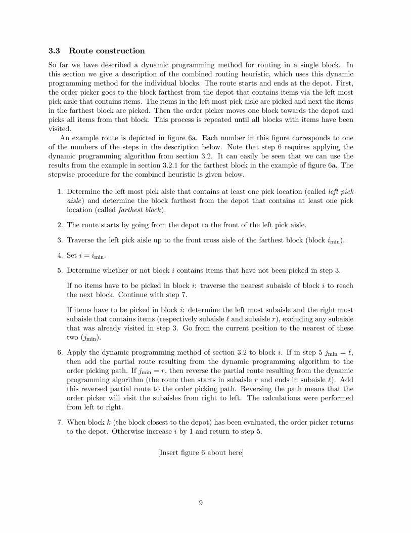
3.3 Route construction

So far we have described a dynamic programming method for routing in a single block. Inthis section we give a description of the combined routing heuristic, which uses this dynamicprogramming method for the individual blocks. The route starts and ends at the depot. First,the order picker goes to the block farthest from the depot that contains items via the left mostpick aisle that contains items. The items in the left most pick aisle are picked and next the itemsin the farthest block are picked. Then the order picker moves one block towards the depot andpicks all items from that block. This process is repeated until all blocks with items have beenvisited.

An example route is depicted in figure 6a. Each number in this figure corresponds to oneof the numbers of the steps in the description below. Note that step 6 requires applying thedynamic programming algorithm from section 3.2. It can easily be seen that we can use theresults from the example in section 3.2.1 for the farthest block in the example of figure 6a. Thestepwise procedure for the combined heuristic is given below.


2. The route starts by going from the depot to the front of the left pick aisle.

3. Traverse the left pick aisle up to the front cross aisle of the farthest block (block imin).

4. Set i = imin.

5. Determine whether or not block i contains items that have not been picked in step 3.

If no items have to be picked in block i: traverse the nearest subaisle of block i to reachthe next block. Continue with step 7.

If items have to be picked in block i: determine the left most subaisle and the right mostsubaisle that contains items (respectively subaisle and subaisle r), excluding any subaislethat was already visited in step 3. Go from the current position to the nearest of thesetwo (jmin).

6. Apply the dynamic programming method of section 3.2 to block i. If in step 5 jmin = ,then add the partial route resulting from the dynamic programming algorithm to theorder picking path. If jmin = r, then reverse the partial route resulting from the dynamicprogramming algorithm (the route then starts in subaisle r and ends in subaisle ). Addthis reversed partial route to the order picking path. Reversing the path means that theorder picker will visit the subaisles from right to left. The calculations were performedfrom left to right.

7. When block k (the block closest to the depot) has been evaluated, the order picker returnsto the depot. Otherwise increase i by 1 and return to step 5.


9

3.4 Improvements

First of all, consider the routing in the block closest to the depot. The starting point for routingin this block is determined by the position where the order picker ends his route through theprevious block. This could lead to a route in which aisles are visited from the left to the right.This implies that the order picker ends his route somewhere at the right of the front cross aisle.After this, a considerable part of the front cross aisle has to be traversed before reaching thedepot. This can be prevented by forcing the route to visit aisles from the right to the left inthe block closest to the depot. It can easily be seen that this change in the heuristic will eitherdecrease travel time or leave the travel time unaltered.

Secondly, consider the path of the order picker from the depot to the farthest block. This pathgoes through the left most pick aisle with pick locations. However one can think of situationswhere it can be advantageous to deviate from this path. In the example of figure 6a, traveltime can be decreased by going through the second pick aisle towards the back of the warehouseinstead of through the first pick aisle. Stated more general, we could create routes such that theorder picker picks items from the left x pick aisles on his way to the farthest block and picksitems from the right n− x pick aisles when returning to the front. The dynamic programmingmethod is applied to the left x subaisles of each block on the way to the back and to the rightn−x subaisles of each block on the way to the front. By optimising over x we obtain a route thatis guaranteed to be shorter or at most as long as the route generated by the original combinedheuristic.

We adapt the combined heuristic to incorporate both improvements suggested in this sectionand call the result the combined+ heuristic. An example route is given in figure 6b. Note thatthe two improvements could also be added to the largest gap and S-shape heuristic. However,the main advantage of these two heuristics is meant to be their ease of use, which would diminishby such substantial alterations. Therefore, we do not alter the other heuristics.

4 A comparison of heuristics

This section compares the optimal and heuristic solutions in a practical order picking system,namely a shelf area. We consider a shelf area where order pickers walk through the warehouseto pick small items, using a small pick cart. The following assumptions are made. The averagewalking speed in both cross aisles and pick aisles is 0.6 metres per second. The centre-to-centredistance between two neighbouring pick aisles is 2.5 metres and no additional time is needed foraisle changing. Cross aisle width is 2.5 metres. Picking of items can be performed simultaneouslyfrom both sides of a pick aisle since the aisles are fairly narrow. Order pickers are assumed towalk through the middle of the pick aisles and cross aisles.

For this type of warehouse we assume the following measures to be representative. Pick aislelength varies between 10 and 30 metres. Each order picker works in a zone consisting of 7 to15 pick aisles. Each picking route has to visit between 10 and 30 locations. These values arebased on observations of numerous actual manual shelf warehouse operations by the authors.We use the extremes of these values for our simulation experiments, which gives eight differentconfigurations. For each configuration, we generate a number of random orders. The locationsof the items in an order are uniformly and independently distributed over the order pickingarea. That is we assume that products are stored randomly in the storage area. No positioningaccording to demand frequencies is used. See for example Caron et al. (1998) for issues involvingnon-random storage.

For each random order, the route length in a warehouse with two cross aisles is calculated for

10

the S-shape, largest gap, aisle-by-aisle, combined and combined+ heuristics and for the optimalalgorithm. Then, an additional cross aisle is added and route length for each of the routingmethods is calculated. Another cross aisle is added, route length is calculated, and so on.Averages are taken over the instances with the same number of cross aisles.

We can distinguish between two ways to increase the number of cross aisles. Firstly, wecan fix the number of storage locations. In this approach the length of the warehouse willincrease if cross aisles are added. Secondly, we could fix the size of the warehouse and addcross aisles by losing storage locations. Since usually in design the amount of storage space isdecided in advance, we choose the first approach. This is consistent with Vaughan and Petersen(1999). The minimum number of cross aisles is two. Such a warehouse with two cross aisleshas one cross aisle in the front and one cross aisle in the back. This restriction is needed sinceall routing methods assume that the order picker is able to enter and leave the subaisles bothfrom the front and from the back. Additional cross aisles are inserted such that the centredistance between any two adjacent cross aisles is equal. Other ways of cross aisle distributionmay be interesting especially in situations where a storage method other than random storageis used. The maximum number of cross aisles is 11 for the experiments. Since the shortest pickaisles in the experiments are 10 metres, having 11 cross aisles means that the shortest subaisleencountered in the experiments is 1 metre. One metre can be considered to be the minimumrack length that is practically feasible in a shelf warehouse.

For each simulation experiment, the necessary number of replications needs to be determinedsuch that the estimate for the mean travel time has a relative error smaller than some γ, for0 < γ < 1. An approximation for the necessary number of replications, such that the relativeerror is smaller than γ with a probability of 1− α, is given in Law and Kelton (1991). For allsituations considered in this paper, a replication size of 2000 orders has appeared to be sufficientto guarantee a relative error of at most 1% with a probability of 95%.

Table 1 gives the average travel time for each combination of the 8 instances, 10 cross aisleconfigurations and 6 routing methods. For each configuration, the best heuristic is indicatedby making the corresponding cell of the table grey. From the table we can see that the S-shape heuristic never had the best performance of the five heuristics. Largest gap had the bestperformance in 5 situations each of which has a layout with two cross aisles. Aisle-by-aisle hadthe best performance in 4 situations, of which 3 equal the travel time of the combined andcombined+ heuristics. The combined+ heuristic gave the best results in 74 of the 80 instances,of which 3 equal the travel time of the aisle-by-aisle and combined heuristics. For each of theheuristics the average calculation time for a single route was less than 0.1 seconds on a 350Mhzcomputer.

[Insert table 1 about here]

If we compare the combined and the S-shape heuristic on theoretical grounds, we can statethat for each individual order combined will give a route that is equal to or shorter than the S-shape route. This is because S-shape entirely traverses every subaisle containing items, whereasthe combined heuristic chooses between entirely traversing the subaisle or returning to the sameside of the subaisle, depending on which gives the shortest travel time. Thus, the combinedheuristic is capable of generating routes that are exactly the same as those of S-shape, however —if possible — it will give shorter order picking routes by returning within subaisles. The differencein performance between S-shape and combined depends on the situation under consideration.For the situations analysed in this paper it holds that average travel time for S-shape is at least7% higher than for combined in warehouses with three cross aisles. The difference between

11

S-shape and combined tends to zero when increasing the number of cross aisles. The percentagedifference between combined and S-shape is smaller if the pick density is high (30 items insteadof 10 items). This is due to the fact that optimal routes generally tend to entirely traverse moreaisles if pick density is higher. Therefore S-shape routes are closer to optimal and the room forimprovement is smaller for the combined heuristic.

A second interesting property of the heuristics is the fact that routes of the aisle-by-aisle,combined and combined+ heuristics are identical for warehouses with two cross aisles. This isdue to the fact that the heuristics use the same system of dynamic programming. Aisle-by-aislecreates routes through all blocks and uses one equivalence class for each cross aisle. Combinedand combined+ apply dynamic programming to each block individually and use two equivalenceclasses, for each cross aisle one. If the warehouse has two cross aisles (i.e. consists of one block)then both heuristics use the same two equivalence classes and consequently give the same routes.

Now let us look at the effect of the improvements for the combined heuristic suggested insection 3.4. Combined and combined+ are the same for warehouses with two cross aisles, becausethe changes only apply to blocks between the depot and the farthest block. For situations withthree cross aisles, the difference between combined and combined+ is minor. The improvementsare however substantial for situations with more than three cross aisles. Average travel time ofcombined was in these cases up to 24.6% over that of combined+.

In the situations with three or more cross aisles, combined+ had the best performance ofthe heuristics for all situations except one. For picklists of 10 items and with three or morecross aisles, the difference between combined+ and optimal is less than 7.5%. For the situationsconsidered in this paper, the size of the gap between combined+ and the optimal algorithm variesbetween 1% and 25% (see table 2). The largest differences occurred for picklists of 30 items.The situations with 7 pick aisles gave a smaller difference between optimal and combined+ thanthe situations with 15 pick aisles. Generally we can say that the gap between optimal andcombined+ tends to be larger if the situation is more complex, i.e. more aisles and/or moreitems.

[Insert table 2 about here]

The observed gap between the best heuristic and the optimal algorithm gives rise to twodifferent approaches for further research: (1) develop better heuristics or (2) use an optimalalgorithm for routing order pickers. Both approaches have their advantages and disadvantages.The heuristics are fairly simple in structure and therefore easy to implement in a practicalsituation. For situations with a large number of cross aisles, it may be worthwhile to analysethe performance of standard routing heuristics for the traveling salesman problem. On the otherhand optimal routing gives significantly shorter routes. However, the logic may be unclear to theorder picker which may cause him to accidentally walk the wrong way or to override the systemand walk the way he thinks is best. Furthermore, in this paper we used a branch-and-boundmethod to calculate the shortest routes. Such a method has unpredictable computation times,which is an undesirable property for practical implementations.

From table 1, we can also see the effect of adding cross aisles to the layout. In general wecan say that travel time decreases if we change the layout from two to three cross aisles. Twoexceptions occur: (1) with largest gap for warehouses with short pick aisles and (2) for a smallwarehouse with many picks. Both exceptions seem intuitively clear. For the first exceptionconsider that if a warehouse has short pick aisles then the distance travelled in the cross aislesaccounts for a relatively large amount of the travel time. This is even more the case whenusing largest gap in warehouses with three or more cross aisles, since routes resulting from this

12

heuristic often traverse cross aisles (except those at the back and front) twice. Consequently, alarge increase in travel time occurs if a third cross aisle is added to the layout. For the secondexception consider a warehouse with a few short pick aisles and many pick locations. Themain advantage of adding cross aisles is that more possibilities arise to route the order picker.However, if the order picker has to visit many locations, then entirely traversing pick aisles isclose to optimal. Any extra cross aisle only increases the warehouse size and therefore traveltimes.

More cross aisles may or may not improve the average time needed to pick an order. Formost situations it holds that adding cross aisles decreases average travel time up to a certainpoint after which average travel time starts increasing again. The optimal number of cross aisleswith respect to travel time seems to depend on the number of pick aisles, the aisle length andthe number of items. Especially aisle length seems to be important in the sense that longeraisles most often require more cross aisles. Important for warehouse design is that more crossaisles implies higher space requirements. Therefore, the cost reductions from adding cross aisleshave to be weighed against increased costs for the building.

5 Concluding remarks

Performances of heuristics in warehouses with two cross aisles have been studied extensively. Inthis paper, we have introduced several methods for routing order pickers in a warehouse withmultiple cross aisles. Two methods, the S-shape and largest gap heuristics, are straight forwardextensions of existing methods for warehouses with two cross aisles. The aisle-by-aisle heuristicwas introduced by Vaughan and Petersen (1999). The combined and combined+ heuristics areintroduced in this paper.

For the majority of the situations (74 of 80) evaluated in this paper, the combined+ heuristichad the best performance of the heuristics. Largest gap was found to be useful in situationswith two cross aisles and low pick densities, which is consistent with Hall (1993).

The performance of the heuristics was also compared to the results of a branch-and-boundprocedure that generates shortest order picking routes. It has to be noted that the gap betweenthis optimal routing method and the best heuristic varies substantially. Implementation of theoptimal procedure in practical situations may however give rise to problems such as unpredictablecomputation times. It could therefore be desirable to improve heuristic performance or find moreefficient methods to calculate shortest routes.

In this paper we considered only situations where products are stored randomly. Otherstorage assignment rules may cause a different ranking among the heuristics. Furthermore, thepositioning of the cross aisles may be an interesting aspect to consider when using non-randomstorage, since there will be much activity in the area with the frequently requested products.

Generally, average travel times decreases when changing the layout from two to three crossaisles. Two exceptions are the situation of a small warehouse with many picks for all rout-ing methods and the situations with short pick aisles for largest gap. More cross aisles mayor may not decrease travel times, depending on the routing method and the situation underconsideration.

6 References

Caron, F., Marchet, G., and Perego, A., 1998, Routing policies and COI-based storage policiesin picker-to-part systems. International Journal of Production Research, 36(3), 713-732.

13

De Koster, R., and Van der Poort, E., 1998, Routing orderpickers in a warehouse: a comparisonbetween optimal and heuristic solutions. IIE Transactions, 30, 469-480.De Koster, R., Van der Poort, E., and Wolters, M., 1999, Efficient orderbatching methods inwarehouses. International Journal of Production Research, 37(7), 1479-1504.Gibson, D. R., and Sharp, G. P., 1992, Order batching procedures. European Journal of Opera-tions Research, 58(1), 57-67.Hall, R. W. H., 1993, Distance approximations for routing manual pickers in a warehouse. IIETransactions, 25(4), 76-87.Goetschalckx, M., and Ratliff, H. D., 1988, Order picking in an aisle. IIE Transactions, 20(1),53-62.Law, A. M., and Kelton, W. D., 1991, Simulation Modeling & Analysis, 2nd ed. (New York:McGraw-Hill, Inc.), chapter 9, pp. 522-581.Little, J. D. C., Murty, K. G., Sweeney, D. W., and Karel, C., 1963, An algorithm for thetraveling salesman problem. Operations Research, 11, 972-989.Petersen, C. G., 1997, An evaluation of order picking routeing policies. International Journalof Operations & Production Management, 17(11), 1098-1111.Petersen, C.G., and Schmenner, R.W., 1999, An evaluation of routing and volume-based storagepolicies in an order picking operation. Decision Sciences, 30(2), 481-501.Ratliff, H. D., and Rosenthal, A. S., 1983, Orderpicking in a rectangular warehouse: A solvablecase of the traveling salesman problem. Operations Research, 31, 507-521.Roodbergen, K. J., and De Koster, R., 1998, Routing orderpickers in a warehouse with multiplecross aisles. In R. J. Graves, L. F. McGinnis, D. J. Medeiros, R. E. Ward and M. R. Wil-helm (eds.), Progress in Material Handling Research: 1998 (Charlotte, NC: Material HandlingInstitute), pp. 451-467.Ruben, R. A., and Jacobs, F. R., 1999, Batch construction heuristics and storage assignmentstrategies for walk/ride and pick systems. Management Science, 45(4), 575-596.Tompkins, J. A., White, J. A., Bozer, Y. A., Frazelle, E. H., Tanchoco, J. M. A., and Trevino,J., 1996, Facilities Planning, 2nd ed. (New York: John Wiley & Sons, Inc.).Vaughan, T. S., and Petersen, C. G., 1999, The effect of warehouse cross aisles on order pickingefficiency. International Journal of Production Research, 37(4), 881-897.

14

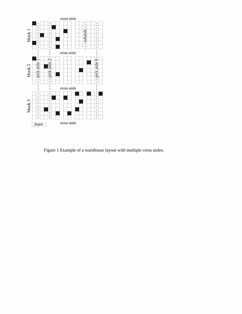
Figure 1 Example of a warehouse layout with multiple cross aisles.

- - -

suba

isle

- - -

- - -

- - -

- - -

- - -

- - -

- - p

ick

aisl

e 1

- - -

- - -

- - -

- - -

- - -

- - -

- - -

- - -

- - -

- - -

- - p

ick

aisl

e 2

- - -

- - -

- - -

- - -

- - -

- - -

- - -

- - -

- - -

- - -

- - p

ick

aisl

e 6

- - -

- - -

- - -

- - -

- - -

a

bc

d e

f i j

hi

f g

i h g h

je

fghgjk

e

a

bc

de

e ee e

g

g

g

f

f

f

h

hhh

k

e

Figure 2 Example routes for four routing methods.

bijbi,j-1 bijbi,j-1

aijai,j-1aij

bij

aij

bij

aij

bij

aij

bij

aijai,j-1

ta tb t1 t2 t3 t4 Figure 3 Transitions used by the combined routing heuristic.

Figure 4 Example situation for the dynamic programming method.

bi1

ai1

bi2 bi3

ai2 ai3

(a) (b)

1

3

2

2

2

6

3

2

2

1

4 4

4 4

Figure 5 Visualisation of the steps taken by the dynamic programming method.

STEP 1 STEP 2 STEP 3

L a1 = t1

L b1 = t3

L a2 = L + t + ta

1 a 4

Lb2 = L + t + ta

1 a 1 L b3 = L + t + ta

2 a 1

bi1

ai1

bi2 bi3

ai2 ai3

bi1

ai1

bi2 bi3

ai2 ai3

bi1

ai1

bi2 bi3

ai2 ai3

bi1

ai1

bi2 bi3

ai2 ai3

bi1

ai1

bi2 bi3

ai2 ai3

7 6

5

6,753,4,5

1,2

Figure 6 Route resulting from applying the combined routing method.

optimal number of cross aisles # aisles length # items 2 3 4 5 6 7 8 9 10 11

7 10 10 138.7 129.7 131.5 135.7 141.7 148.0 155.5 162.0 169.6 177.4 7 10 30 186.6 191.4 198.6 207.1 216.3 224.9 235.0 243.2 252.8 261.6 15 10 10 219.6 202.0 201.4 205.2 211.4 218.2 226.7 233.8 242.2 251.0 15 10 30 337.5 314.3 311.6 315.7 324.5 333.4 346.1 355.6 368.7 381.4 7 30 10 269.6 222.9 211.1 209.0 211.4 215.8 221.3 227.4 233.9 240.2 7 30 30 398.3 361.1 342.9 336.5 333.8 334.2 337.0 340.8 345.0 349.7 15 30 10 377.3 308.0 290.9 287.7 289.3 293.5 299.2 305.4 312.0 318.5 15 30 30 665.5 540.6 495.9 479.8 473.3 472.8 475.9 480.7 486.0 491.7

Largest gap number of cross aisles

# aisles length # items 2 3 4 5 6 7 8 9 10 11 7 10 10 146.6 156.9 164.6 169.3 176.3 181.9 187.4 194.7 201.9 209.3 7 10 30 208.6 240.9 273.9 303.5 330.3 348.6 363.4 379.6 394.4 408.4 15 10 10 227.3 265.2 287.2 296.2 305.7 312.2 317.1 324.6 331.4 338.4 15 10 30 357.5 413.5 484.5 552.1 614.6 660.1 692.3 724.7 750.1 776.3 7 30 10 295.1 259.9 250.7 246.3 247.4 250.3 254.5 259.7 264.9 270.6 7 30 30 451.7 424.7 425.7 435.9 446.9 456.1 464.1 472.2 478.4 488.7 15 30 10 401.0 377.6 379.1 377.2 379.5 382.4 386.6 390.6 395.2 400.6 15 30 30 715.6 646.0 665.4 705.2 746.3 779.9 805.0 826.5 842.8 863.7

S-shape number of cross aisles


Aisle-by-aisle number of cross aisles


Combined number of cross aisles


Combined+ number of cross aisles


Table 1 Average travel time for six routing methods.

Percentage difference number of cross aisles # aisles length # items 2 3 4 5 6 7 8 9 10 11

7 10 10 7.1 2.7 3.6 3.3 3.0 2.8 2.5 2.4 2.2 2.07 10 30 2.9 2.4 13.2 12.0 12.9 12.6 10.9 10.6 9.4 8.5

15 10 10 7.1 2.5 6.5 7.6 7.7 7.4 6.8 6.6 6.1 5.515 10 30 5.7 2.9 19.8 20.2 23.7 24.6 22.9 22.9 21.4 19.97 30 10 13.0 5.6 3.9 2.8 2.2 1.9 1.8 1.5 1.4 1.47 30 30 5.2 5.7 10.6 8.7 8.6 7.9 7.3 6.7 6.3 6.0

15 30 10 13.2 4.9 4.9 4.5 4.1 3.7 3.6 3.4 3.2 3.215 30 30 10.1 6.8 14.5 12.5 13.8 13.5 13.0 12.7 12.2 12.0

Table 2 Percentage difference in average travel time between the combined+ and the optimal routing method.

Documents

Routing methods for warehouses with multiple cross aisles · Routing methods for warehouses with multiple cross aisles ... Routing methods for warehouses with multiple ... all items