Embed Size (px)
Citation preview
1
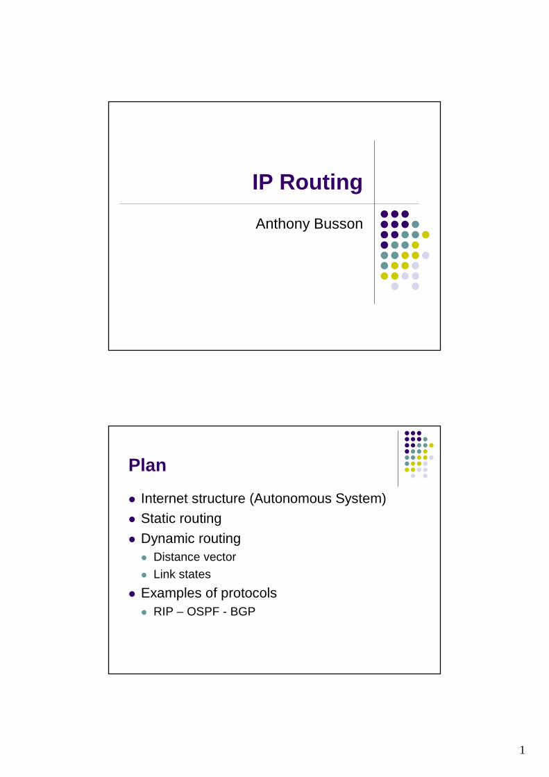
IP Routing
Anthony Busson
Plan
� Internet structure (Autonomous System)� Static routing
� Dynamic routing� Distance vector� Link states
� Examples of protocols� RIP – OSPF - BGP
2
AS u
AS w
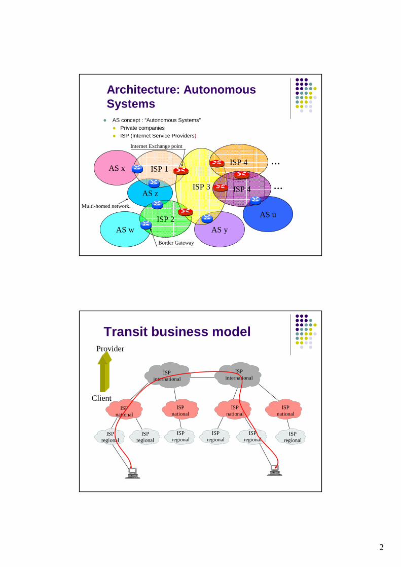
� AS concept : “Autonomous Systems”
� Private companies� ISP (Internet Service Providers)
Architecture: Autonomous Systems
AS x
AS z
AS y
ISP 1
ISP 2
ISP 3
Multi-homed network.
Border Gateway
Internet Exchange point
ISP 4 ...
ISP 4 ...
Transit business model
ISPregional
ISPregional
ISPregional
ISPregional
ISPregional
ISPregional
ISPnational
ISPnational
ISPnational
ISPnational
ISPinternational
ISPinternational
Client
Provider
3
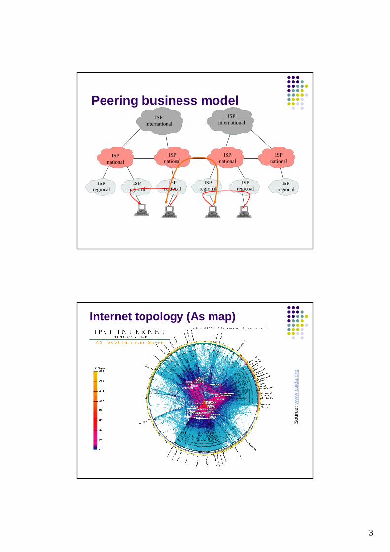
Peering business model
ISPregional
ISPregional
ISPregional
ISPregional
ISPregional
ISPregional
ISPnational
ISPnational
ISPnational
ISPnational
ISPinternational
ISPinternational
Internet topology (As map)
Source: www.caida.org
4
Routing:a computer
direct – indirect routing
� When a computer emits a packet to a given IP destination address� It performs a logical bitwise operation « AND » between its
own mask and the IP destination address� It compares the result with its own network address
� If they are identical: direct routing (an ARP request is sent to the destination).
� If they are not identical: indirect routing (the packet will be sent to the router: the ARP request is sent to the router).
ARP: Address Resolution ProtocolARP: Address Resolution Protocol
5
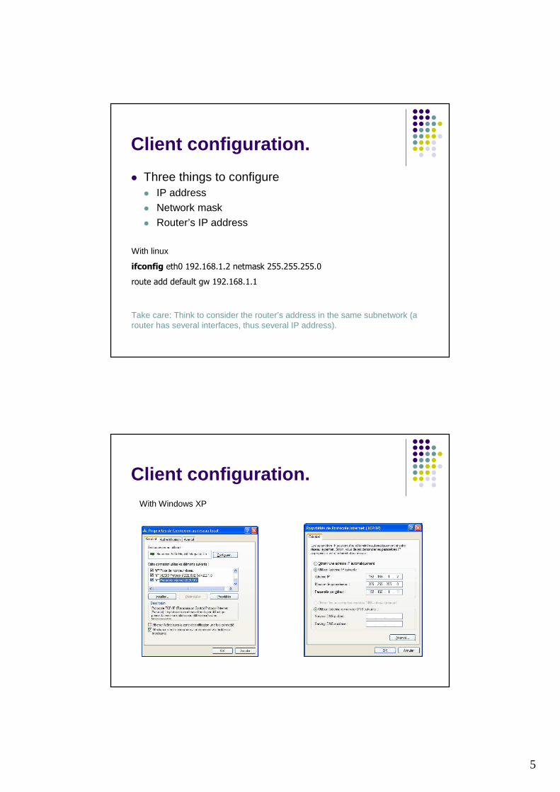
Client configuration.
� Three things to configure� IP address� Network mask� Router’s IP address
With linux
ifconfig eth0 192.168.1.2 netmask 255.255.255.0
route add default gw 192.168.1.1
Take care: Think to consider the router’s address in the same subnetwork (a router has several interfaces, thus several IP address).
Client configuration.With Windows XP
6
Routing table andstatic routing
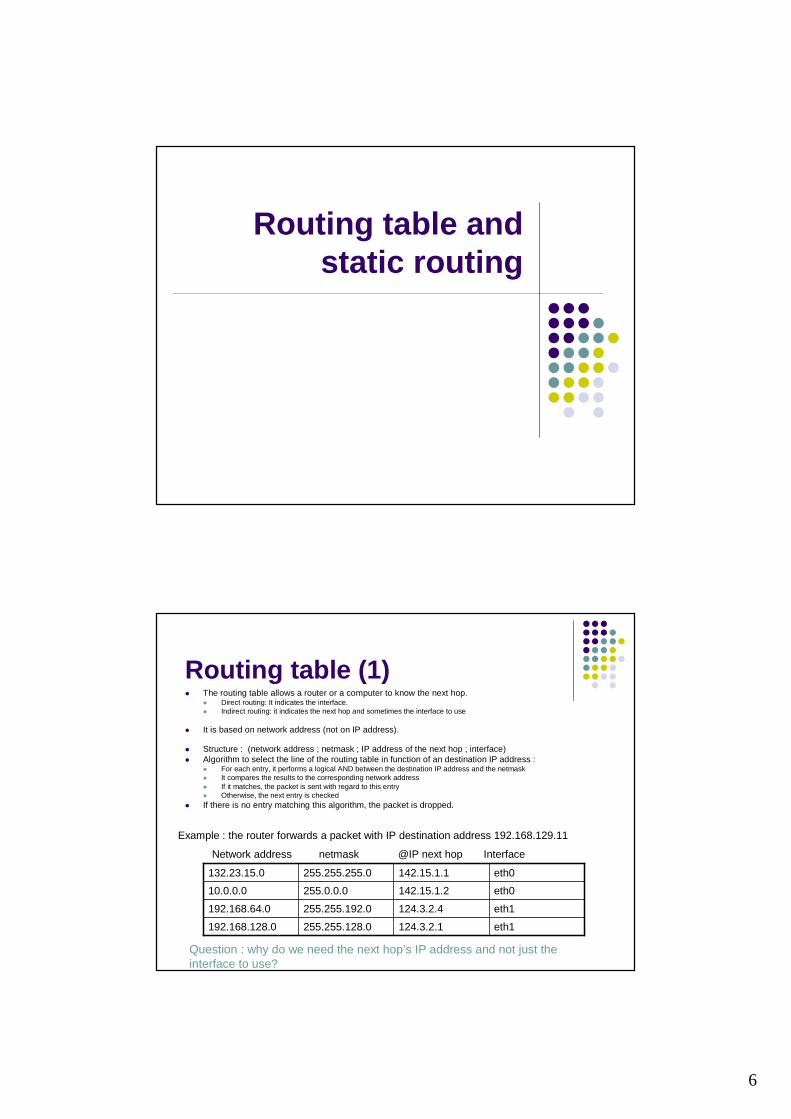
Routing table (1)� The routing table allows a router or a computer to know the next hop.
� Direct routing: It indicates the interface. � Indirect routing: it indicates the next hop and sometimes the interface to use
� It is based on network address (not on IP address).
� Structure : (network address ; netmask ; IP address of the next hop ; interface)� Algorithm to select the line of the routing table in function of an destination IP address :
� For each entry, it performs a logical AND between the destination IP address and the netmask� It compares the results to the corresponding network address� If it matches, the packet is sent with regard to this entry� Otherwise, the next entry is checked
� If there is no entry matching this algorithm, the packet is dropped.
Example : the router forwards a packet with IP destination address 192.168.129.11
eth1124.3.2.1255.255.128.0192.168.128.0
eth1124.3.2.4255.255.192.0192.168.64.0
eth0142.15.1.2255.0.0.010.0.0.0
eth0142.15.1.1255.255.255.0132.23.15.0
Network address netmask @IP next hop Interface
Question : why do we need the next hop’s IP address and not just the interface to use?
7
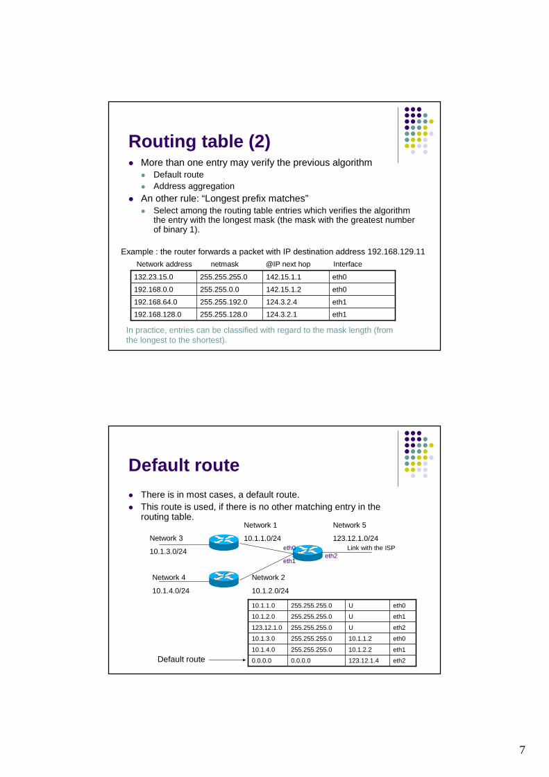
Routing table (2)� More than one entry may verify the previous algorithm
� Default route� Address aggregation
� An other rule: “Longest prefix matches”� Select among the routing table entries which verifies the algorithm
the entry with the longest mask (the mask with the greatest number of binary 1).
Example : the router forwards a packet with IP destination address 192.168.129.11
eth1124.3.2.1255.255.128.0192.168.128.0
eth1124.3.2.4255.255.192.0192.168.64.0
eth0142.15.1.2255.255.0.0192.168.0.0
eth0142.15.1.1255.255.255.0132.23.15.0
Network address netmask @IP next hop Interface
In practice, entries can be classified with regard to the mask length (from the longest to the shortest).
Default route� There is in most cases, a default route.� This route is used, if there is no other matching entry in the
routing table.
Link with the ISP
Network 1
10.1.1.0/24
Network 2
10.1.2.0/24
Network 4
10.1.4.0/24
Network 3
10.1.3.0/24 eth0
eth1eth2
eth2U255.255.255.0123.12.1.0
eth110.1.2.2255.255.255.010.1.4.0
eth2123.12.1.40.0.0.00.0.0.0
eth010.1.1.2255.255.255.010.1.3.0
eth1U255.255.255.010.1.2.0
eth0U255.255.255.010.1.1.0
Network 5
123.12.1.0/24
Default route
8
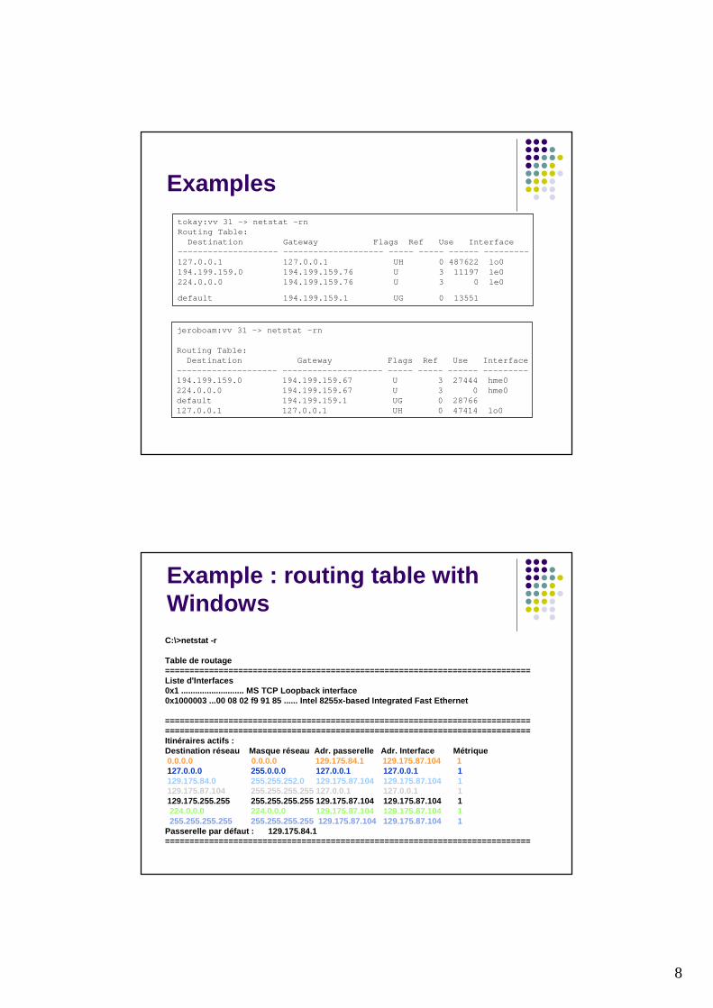
Examplestokay:vv 31 -> netstat -rnRouting Table:
Destination Gateway Flags Ref Use Interface-------------------- -------------------- ----- ----- ------ ---------127.0.0.1 127.0.0.1 UH 0 487622 lo0194.199.159.0 194.199.159.76 U 3 11197 le0224.0.0.0 194.199.159.76 U 3 0 le0
default 194.199.159.1 UG 0 13551
jeroboam:vv 31 -> netstat -rn
Routing Table:Destination Gateway Flags Ref Use Interface
-------------------- -------------------- ----- ----- ------ ---------194.199.159.0 194.199.159.67 U 3 27444 hme0224.0.0.0 194.199.159.67 U 3 0 hme0default 194.199.159.1 UG 0 28766127.0.0.1 127.0.0.1 UH 0 47414 lo0
Example : routing table withWindowsC:\>netstat -r
Table de routage===========================================================================Liste d'Interfaces0x1 ........................... MS TCP Loopback inte rface0x1000003 ...00 08 02 f9 91 85 ...... Intel 8255x-b ased Integrated Fast Ethernet
======================================================================================================================================================Itinéraires actifs :Destination réseau Masque réseau Adr. passerell e Adr. Interface Métrique0.0.0.0 0.0.0.0 129.175.84.1 129.175.87.104 1127.0.0.0 255.0.0.0 127.0.0.1 127.0.0.1 1129.175.84.0 255.255.252.0 129.175.87.104 129.175.87.104 1129.175.87.104 255.255.255.255 127.0.0.1 127.0.0.1 1129.175.255.255 255.255.255.255 129.175.87.104 129.175.87.104 1224.0.0.0 224.0.0.0 129.175.87.104 129.175.87.104 1255.255.255.255 255.255.255.255 129.175.87.104 129.175.87.104 1
Passerelle par défaut : 129.175.84.1===========================================================================
9
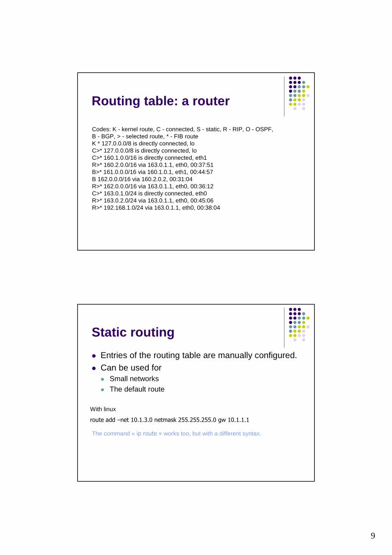
Routing table: a router
Codes: K - kernel route, C - connected, S - static, R - RIP, O - OSPF,B - BGP, > - selected route, * - FIB routeK * 127.0.0.0/8 is directly connected, loC>* 127.0.0.0/8 is directly connected, loC>* 160.1.0.0/16 is directly connected, eth1R>* 160.2.0.0/16 via 163.0.1.1, eth0, 00:37:51B>* 161.0.0.0/16 via 160.1.0.1, eth1, 00:44:57B 162.0.0.0/16 via 160.2.0.2, 00:31:04R>* 162.0.0.0/16 via 163.0.1.1, eth0, 00:36:12C>* 163.0.1.0/24 is directly connected, eth0R>* 163.0.2.0/24 via 163.0.1.1, eth0, 00:45:06R>* 192.168.1.0/24 via 163.0.1.1, eth0, 00:38:04
Static routing
� Entries of the routing table are manually configured.
� Can be used for� Small networks� The default route
With linux
route add –net 10.1.3.0 netmask 255.255.255.0 gw 10.1.1.1
The command « ip route » works too, but with a different syntax.
10
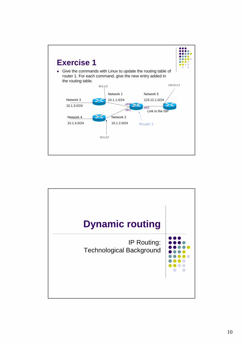
Exercise 1� Give the commands with Linux to update the routing table of
router 1. For each command, give the new entry added in the routing table.
Link to the ISP
Network 1
10.1.1.0/24
Network 2
10.1.2.0/24
Network 4
10.1.4.0/24
Network 3
10.1.3.0/24 eth0
eth1eth2
Network 5
123.12.1.0/24
Router 1
10.1.1.2
10.1.2.2
123.12.1.2
Dynamic routing
IP Routing:Technological Background
11
Routing protocolDefinition and requirements� A routing protocol is a mechanism used to build and update the routing
table. It relies on information exchanged between the routers. � The routing protocol specifies:
� The method of exchanging messages between routers (frequency, scope, transport protocol, etc.)
� The format and the content of the messages exchanged between the router� The algorithm used to compute the routing table (from the set of messages
received from the routers)
� A routing protocol should be (ideally)� Efficient : compute the best path for each destination� Simple : quite easy to implement� Flexible : adapt quickly to topology changes� Not greedy : it shouldn’t consume too much bandwidth� Converge quickly
Dynamic routing
� Building and update of the routing table.� Routers send messages to announce and
learn the route to the different subnetwork.� The router’s interface have to be manually
configurerd (IP address and netmask).
� Two kind of routing protocols in the Internet:� Distance Vector� Link States
12
Distance vectorprotocol
Distance vector
� Distance vector protocols are based on mechanisms developed by Bellman-Ford.
� Routes are announced through « Vector » with two fields (destination, distance) where the distance is a metric (number of hops for instance).
� Routers regularly broadcast to their direct neighbors a simplified version of their routing table (destination, distance).
� Upon receiving a vector from a neighbor, a router compares the routes of the vector with the routes of its routing table and update it.
13
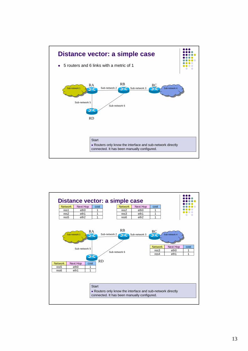
Distance vector: a simple case
� 5 routers and 6 links with a metric of 1
RA RB RC
RD
Sub-network 4Sub-network 4
Sub-network 1Sub-network 1
Sub-network 6
Sub-network 2 Sub-network 3
Sub-network 5
Start� Routers only know the interface and sub-network directly connected. It has been manually configured.
Distance vector: a simple case
RA RB RC
RD
Sub-network 4Sub-network 4
Sub-network 1Sub-network 1
Sub-network 6
Sub-network 2 Sub-network 3
Sub-network 5Network Next Hop
res3 eth0cost
1res4 eth1 1
Network Next Hopres2 eth0
cost1
res3 eth1 1
Network Next Hopres1 eth0
cost1
res2 eth1 1
Network Next Hopres5 eth0
cost1
res6 eth1 1
res5 eth2 1 res6 eth2 1
Start� Routers only know the interface and sub-network directly connected. It has been manually configured.
14
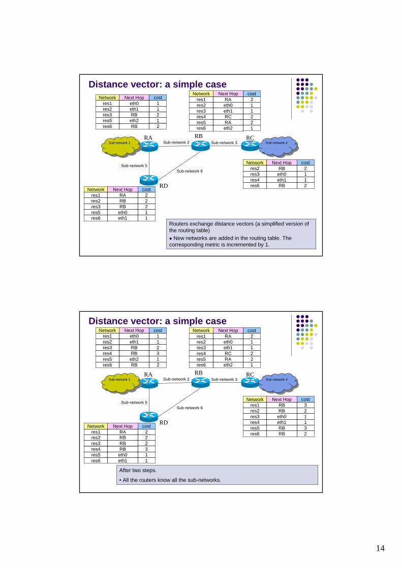
Distance vector: a simple case
RA RB RC
RD
Sub-network 4Sub-network 4
Sub-network 1Sub-network 1
Sub-network 6
Sub-network 2 Sub-network 3
Sub-network 5
Routers exchange distance vectors (a simplified version of the routing table)� New networks are added in the routing table. The corresponding metric is incremented by 1.
Network Next Hop cost
res3 eth0 1res4 eth1 1
Network Next Hopres1 eth0
cost1
res2 eth1 1
Network Next Hop cost
res5 eth0 1res6 eth1 1
res2 RB 2
res1 RA 2
res5 eth2 1
res2 RB 2res3 RB 2
res3 RB 2
res6 RB 2
Network Next Hop cost
res2 eth0 1res3 eth1 1res4 RC 2
res6 eth2 1
res1 RA 2
res5 RA 2
res6 RB 2
Distance vector: a simple case
RA RB RC
RD
Sub-network 4Sub-network 4
Sub-network 1Sub-network 1
Sub-network 6
Sub-network 2 Sub-network 3
Sub-network 5
After two steps.
• All the routers know all the sub-networks.
Network Next Hop cost
res3 eth0 1res4 eth1 1
Network Next Hopres1 eth0
cost1
res2 eth1 1
Network Next Hop cost
res5 eth0 1res6 eth1 1
res1 RB 3res2 RB 2
res1 RA 2
res5 eth2 1
res2 RB 2res3 RB 2
res3 RB 2
res6 RB 2
Network Next Hop cost
res2 eth0 1res3 eth1 1res4 RC 2
res6 eth2 1
res1 RA 2
res5 RA 2
res5 RB 3
res4 RB 3
res4 RB 3
res6 RB 2
15
Distance vector: a simple case
RA RB RC
RD
Sub-network 4Sub-network 4
Sub-network 1Sub-network 1
Sub-network 6
Sub-network 2 Sub-network 3
Sub-network 5
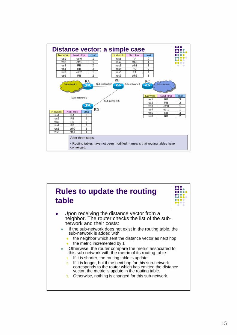
After three steps.
• Routing tables have not been modified. It means that routing tables have converged.
Network Next Hop cost
res3 eth0 1res4 eth1 1
Network Next Hopres1 eth0
cost1
res2 eth1 1
Network Next Hop cost
res5 eth0 1res6 eth1 1
res1 RB 3res2 RB 2
res1 RA 2
res5 eth2 1
res2 RB 2res3 RB 2
res3 RB 2
res6 RB 2
Network Next Hop cost
res2 eth0 1res3 eth1 1res4 RC 2
res6 eth2 1
res1 RA 2
res5 RA 2
res5 RB 3
res4 RB 3
res4 RB 3
res6 RB 2
Rules to update the routingtable
� Upon receiving the distance vector from a neighbor. The router checks the list of the sub-network and their costs:
� If the sub-network does not exist in the routing table, the sub-network is added with
� the neighbor which sent the distance vector as next hop� the metric incremented by 1
� Otherwise, the router compare the metric associated to this sub-network with the metric of its routing table
1. If it is shorter, the routing table is update. 2. If it is longer, but if the next hop for this sub-network
corresponds to the router which has emitted the distance vector, the metric is update in the routing table.
3. Otherwise, nothing is changed for this sub-network.
16
Distance vector – link failure
RA RB RC
RD
Sub-network 4Sub-network 4
Sub-network 1Sub-network 1
Sub-network 6
Sub-network 2Sub-network 3
Sub-network5
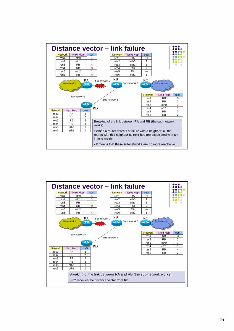
Breaking of the link between RA and RB (the sub-network works).
• When a router detects a failure with a neighbor, all the routes with this neighbor as next hop are associated with an infinite metric.
• It means that these sub-networks are no more reachable.
Network Next Hop cost
res3 eth0 1res4 eth1 1
Network Next Hopres1 eth0
cost1
res2 eth1 1
Network Next Hop cost
res5 eth0 1res6 eth1 1
res1 RB 3res2 RB 2
res1 RA 2
res5 eth2 1
res2 RB 2res3 RB 2
res3 RB ∞
res6 RB ∞
Network Next Hop cost
res2 eth0 1res3 eth1 1res4 RC 2
res6 eth2 1
res1 RA ∞
res5 RA ∞
res5 RB 3
res4 RB ∞
res4 RB 3
res6 RB 2
Distance vector – link failure
RA RB RC
RD
Sub-network 4Sub-network 4
Sub-network 1Sub-network 1
Sub-network 6
Sub-network 2Sub-network 3
Sub-network 5
Breaking of the link between RA and RB (the sub-network works).
• RC receives the distance vector from RB.
Network Next Hop cost
res3 eth0 1res4 eth1 1
Network Next Hopres1 eth0
cost1
res2 eth1 1
Network Next Hop coût
res5 eth0 1res6 eth1 1
res1 RB ∞res2 RB 2
res1 RA 2
res5 eth2 1
res2 RB 2res3 RB 2
res3 RB ∞
res6 RB ∞
Network Next Hop cost
res2 eth0 1res3 eth1 1res4 RC 2
res6 eth2 1
res1 RA ∞
res5 RA ∞
res5 RB ∞
res4 RB ∞
res4 RB 3
res6 RB 2
17
Distance vector – link failure
RA RB RC
RD
Sub-network 4Sub-network 4
Sub-network 1Sub-network 1
Sub-network 6
Sub-network 2Sub-network 3
Sub-network 5
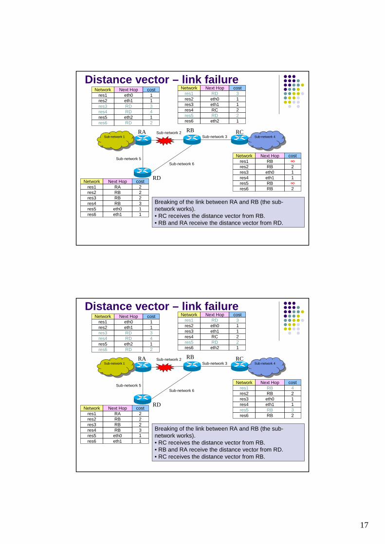
Breaking of the link between RA and RB (the sub-network works). • RC receives the distance vector from RB.• RB and RA receive the distance vector from RD.
Network Next Hop cost
res3 eth0 1res4 eth1 1
Network Next Hopres1 eth0
cost1
res2 eth1 1
Network Next Hop cost
res5 eth0 1res6 eth1 1
res1 RB ∞res2 RB 2
res1 RA 2
res5 eth2 1
res2 RB 2res3 RB 2
res3 RD 3
res6 RD 2
Network Next Hop cost
res2 eth0 1res3 eth1 1res4 RC 2
res6 eth2 1
res1 RD 3
res5 RD 2
res5 RB ∞
res4 RD 4
res4 RB 3
res6 RB 2
Distance vector – link failure
RA RB RC
RD
Sub-network 4Sub-network 4
Sub-network 1Sub-network 1
Sub-network 6
Sub-network 2Sub-network 3
Sub-network 5
Breaking of the link between RA and RB (the sub-network works). • RC receives the distance vector from RB.• RB and RA receive the distance vector from RD.• RC receives the distance vector from RB.
Network Next Hop cost
res3 eth0 1res4 eth1 1
Network Next Hopres1 eth0
cost1
res2 eth1 1
Network Next Hop cost
res5 eth0 1res6 eth1 1
res1 RB 4res2 RB 2
res1 RA 2
res5 eth2 1
res2 RB 2res3 RB 2
res3 RD 3
res6 RD 2
Network Next Hop cost
res2 eth0 1res3 eth1 1res4 RC 2
res6 eth2 1
res1 RD 3
res5 RD 2
res5 RB 3
res4 RD 4
res4 RB 3
res6 RB 2
18
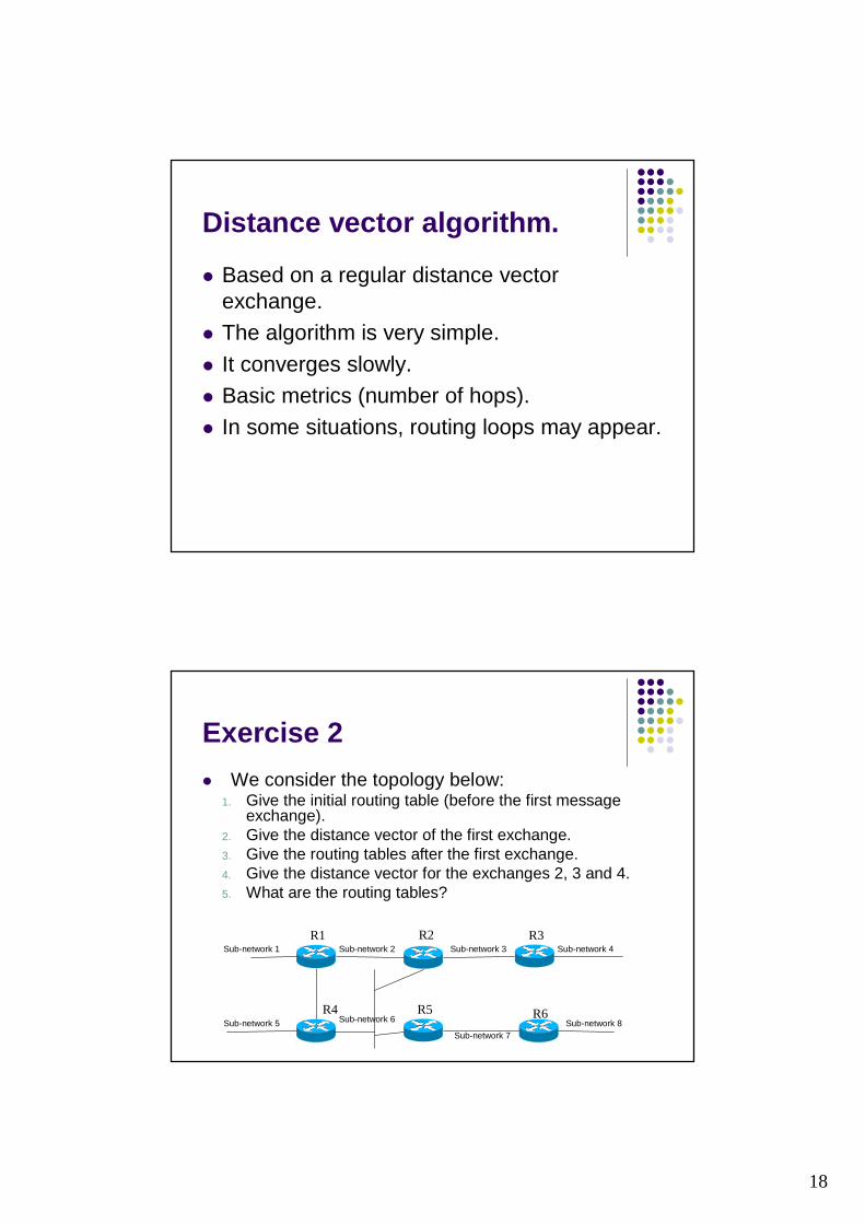
Distance vector algorithm.
� Based on a regular distance vector exchange.
� The algorithm is very simple.
� It converges slowly.� Basic metrics (number of hops).� In some situations, routing loops may appear.
Exercise 2
� We consider the topology below:1. Give the initial routing table (before the first message
exchange).2. Give the distance vector of the first exchange.3. Give the routing tables after the first exchange.4. Give the distance vector for the exchanges 2, 3 and 4. 5. What are the routing tables?
R1 R2
Sub-network 7
Sub-network 2 Sub-network 3Sub-network 1 Sub-network 4
Sub-network 5 Sub-network 6 Sub-network 8R4 R5 R6
R3
19
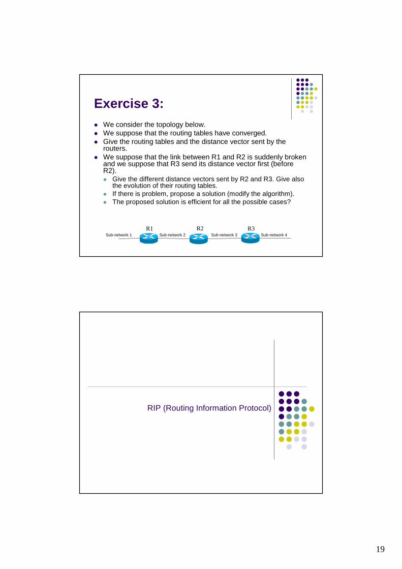
Exercise 3:� We consider the topology below.� We suppose that the routing tables have converged. � Give the routing tables and the distance vector sent by the
routers.� We suppose that the link between R1 and R2 is suddenly broken
and we suppose that R3 send its distance vector first (before R2).� Give the different distance vectors sent by R2 and R3. Give also
the evolution of their routing tables.� If there is problem, propose a solution (modify the algorithm).� The proposed solution is efficient for all the possible cases?
R1 R2Sub-network 2 Sub-network 3Sub-network 1 Sub-network 4
R3
RIP (Routing Information Protocol)
20
� History:� Originally defined by Xerox to be used in the XNS architecture
(Xerox Network Systems). It was then recovered by the Internet community, RFC 1058 (1988).
� RIPv2 (RFC2453) proposed in late 1998� Characteristics:
� Simple distance vector protocol� Metric: Number of hops� VLSM introduced in RIPv2
� Advantages :� Simple and well adapted to small networks
� Limitations:� Metric: only the number of hops Maximal diameter: 15 hops.
� Two mechanisms to avoid loops� Split Horizon� Triggered update
RIP: Summary
RIP Database
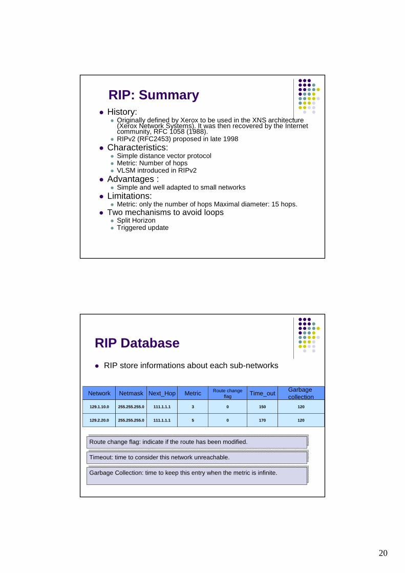
� RIP store informations about each sub-networks
Network Netmask Next_Hop Route change flag Time_out
Garbagecollection
129.1.10.0 255.255.255.0 111.1.1.1 0 150 120
129.2.20.0 255.255.255.0 111.1.1.1 0 170 120
Metric
3
5
Route change flag: indicate if the route has been modified.Route change flag: indicate if the route has been modified.
Timeout: time to consider this network unreachable.Timeout: time to consider this network unreachable.
Garbage Collection: time to keep this entry when the metric is infinite.Garbage Collection: time to keep this entry when the metric is infinite.
21
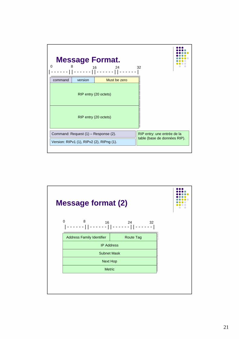
Message Format.| - - - - - - | | - - - - - - | | - - - - - - | | - - - - - - |
RIP entry (20 octets)RIP entry (20 octets)
RIP entry (20 octets)RIP entry (20 octets)
0 8 16 24 32
commandcommand versionversion Must be zeroMust be zero
Command: Request (1) – Response (2).
Version: RIPv1 (1), RIPv2 (2), RIPng (1).
RIP entry: une entrée de la table (base de données RIP).
Message format (2)
MetricMetric
Next HopNext Hop
Subnet MaskSubnet Mask
| - - - - - - | | - - - - - - | | - - - - - - | | - - - - - - |
IP AddressIP Address
Address Family IdentifierAddress Family Identifier
0 8 16 24 32
Route TagRoute Tag
22
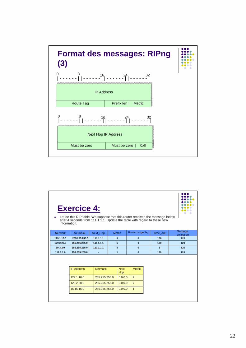
Format des messages: RIPng(3)
| - - - - - - | | - - - - - - | | - - - - - - | | - - - - - - |
Route TagRoute Tag Prefix len | MetricPrefix len | Metric
IP AddressIP Address
0 8 16 24 32
| - - - - - - | | - - - - - - | | - - - - - - | | - - - - - - |
Must be zeroMust be zero Must be zero | 0xffMust be zero | 0xff
Next Hop IP AddressNext Hop IP Address
0 8 16 24 32
Exercice 4:� Let be this RIP table. We suppose that this router received the message below
after 4 seconds from 111.1.1.1. Update the table with regard to these new information.
Network Netmask Next_Hop Route change flag Time_outGarbagecollection
129.1.10.0 255.255.255.0 111.1.1.1 0 150 120
129.2.20.0 255.255.255.0 111.1.1.1 0 170 120
Metric
3
5
19.3.2.0 255.255.255.0 111.1.1.1 0 3 1205
111.1.1.0 255.255.255.0 - 0 180 1201
10.0.0.0255.255.255.015.15.15.0
70.0.0.0255.255.255.0129.2.20.0
20.0.0.0255.255.255.0129.1.10.0
MetricNextHop
NetmaskIP Address
23
Link-states Algorithm
© CentralWeb - 1998 52
Link States algorithm.
� Each router is responsible for the discovering of the � The sub-network directly connected� Routers directly connected
� Each router build a « Link State » packet (LSP) that contains the lists of the links to the neighbors and the associated costs.
� The LSP is broadcasted in the whole network.
� Each router keeps in a database the most recent LSP sent by each router.
� Therefore, each router knows the whole toplogy of the network. It computes the best path to each sub-network and update the routing table.
24
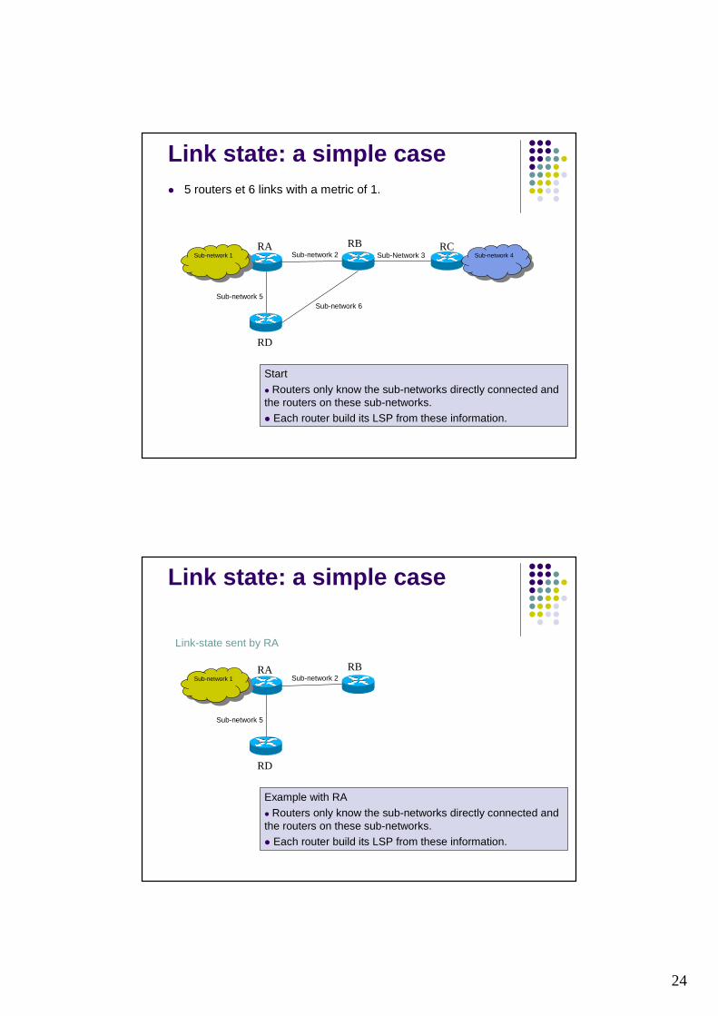
Link state: a simple case� 5 routers et 6 links with a metric of 1.
RA RB RC
RD
Sub-network 4Sub-network 4
Sub-network 1Sub-network 1
Sub-network 6
Sub-network 2 Sub-Network 3
Sub-network 5
Start
� Routers only know the sub-networks directly connected andthe routers on these sub-networks. � Each router build its LSP from these information.
Link state: a simple case
RA RB
RD
Sub-network 1Sub-network 1 Sub-network 2
Sub-network 5
Example with RA
� Routers only know the sub-networks directly connected andthe routers on these sub-networks. � Each router build its LSP from these information.
Link-state sent by RA
25
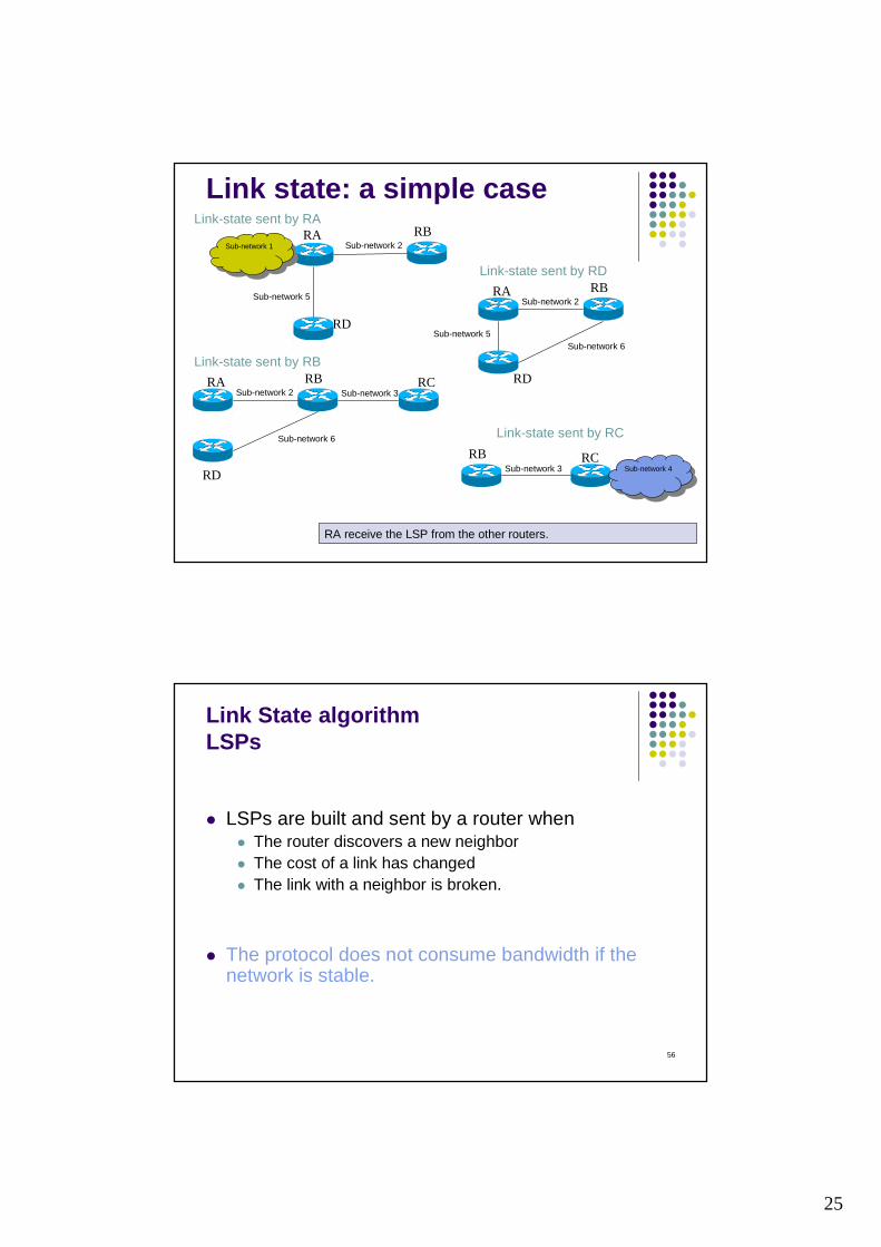
Link state: a simple case
RA receive the LSP from the other routers.
RA RB RC
RD
Sub-network 6
Sub-network 2 Sub-network 3
RA RB
RD
Sub-network 1Sub-network 1 Sub-network 2
Sub-network 5
RB RCSub-network 4
Sub-network 4Sub-network 3
Link-state sent by RC
Link-state sent by RB
Link-state sent by RA
RA RB
RD
Sub-network 2
Link-state sent by RD
Sub-network 6Sub-network 5
© CentralWeb - 1998 56
Link State algorithmLSPs
� LSPs are built and sent by a router when� The router discovers a new neighbor� The cost of a link has changed� The link with a neighbor is broken.
� The protocol does not consume bandwidth if the network is stable.
26
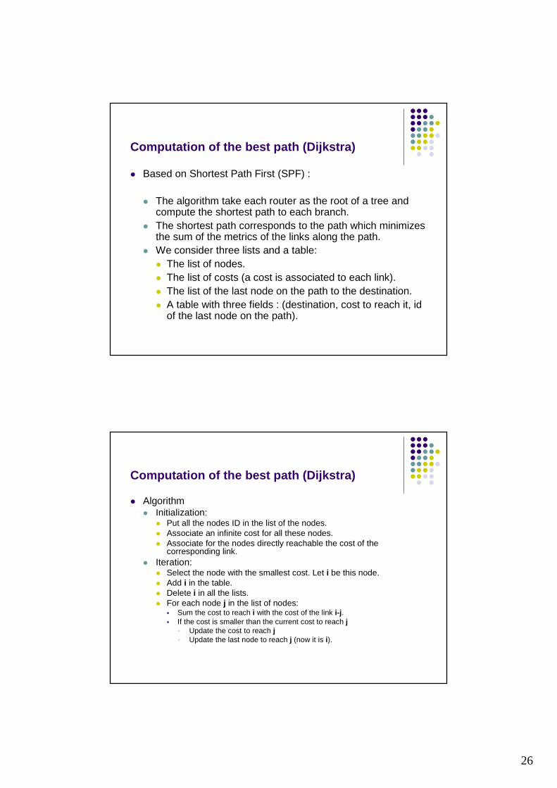
Computation of the best path (Dijkstra)
� Based on Shortest Path First (SPF) :
� The algorithm take each router as the root of a tree and compute the shortest path to each branch.
� The shortest path corresponds to the path which minimizes the sum of the metrics of the links along the path.
� We consider three lists and a table:� The list of nodes. � The list of costs (a cost is associated to each link). � The list of the last node on the path to the destination. � A table with three fields : (destination, cost to reach it, id
of the last node on the path).
Computation of the best path (Dijkstra)
� Algorithm� Initialization:
� Put all the nodes ID in the list of the nodes.� Associate an infinite cost for all these nodes. � Associate for the nodes directly reachable the cost of the
corresponding link.� Iteration:
� Select the node with the smallest cost. Let i be this node. � Add i in the table.� Delete i in all the lists.� For each node j in the list of nodes:
� Sum the cost to reach i with the cost of the link i-j.� If the cost is smaller than the current cost to reach j
� Update the cost to reach j� Update the last node to reach j (now it is i).
27
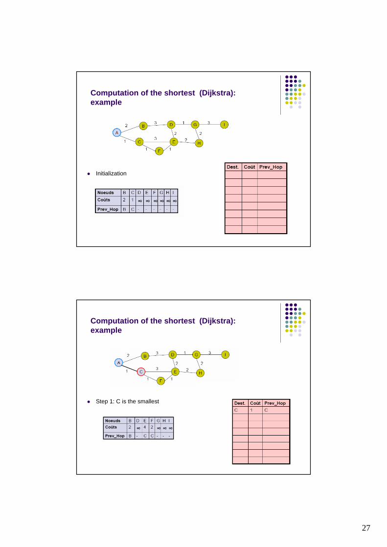
Computation of the shortest (Dijkstra):example
� Initialization
Computation of the shortest (Dijkstra):example
� Step 1: C is the smallest
28
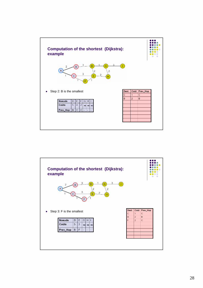
Computation of the shortest (Dijkstra):example
� Step 2: B is the smallest
Computation of the shortest (Dijkstra):example
� Step 3: F is the smallest
29
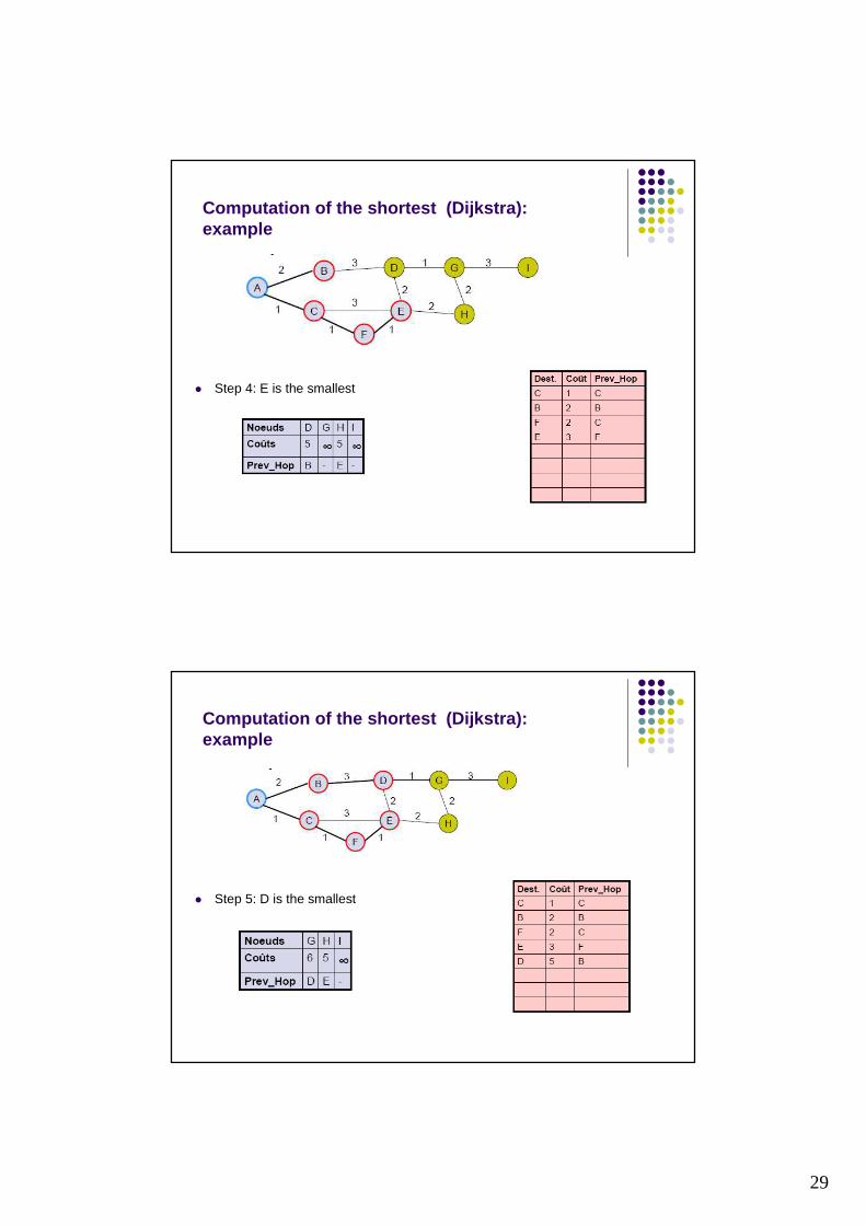
Computation of the shortest (Dijkstra):example
� Step 4: E is the smallest
Computation of the shortest (Dijkstra):example
� Step 5: D is the smallest
30
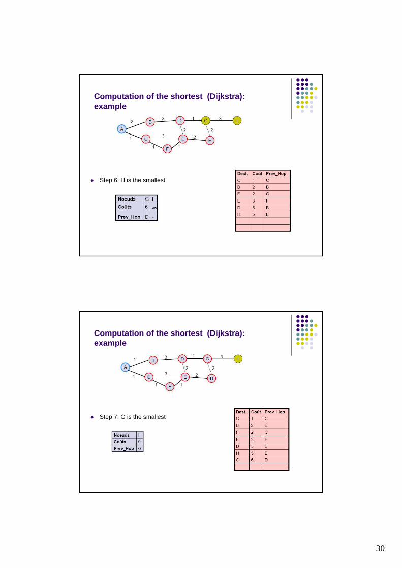
Computation of the shortest (Dijkstra):example
� Step 6: H is the smallest
Computation of the shortest (Dijkstra):example
� Step 7: G is the smallest
31
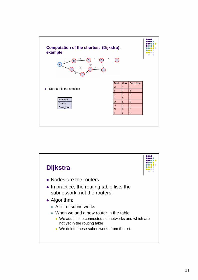
Computation of the shortest (Dijkstra):example
� Step 8: I is the smallest
Dijkstra
� Nodes are the routers� In practice, the routing table lists the
subnetwork, not the routers.
� Algorithm:� A list of subnetworks� When we add a new router in the table
� We add all the connected subnetworks and which are not yet in the routing table
� We delete these subnetworks from the list.
32
© CentralWeb - 1998 69
Link-state algorithm
� Benefit of the Link State algorithm:� It converges quickly� It does not create routing loop
� Drawback of the Link State algorithm:� Complexity� Size of the database
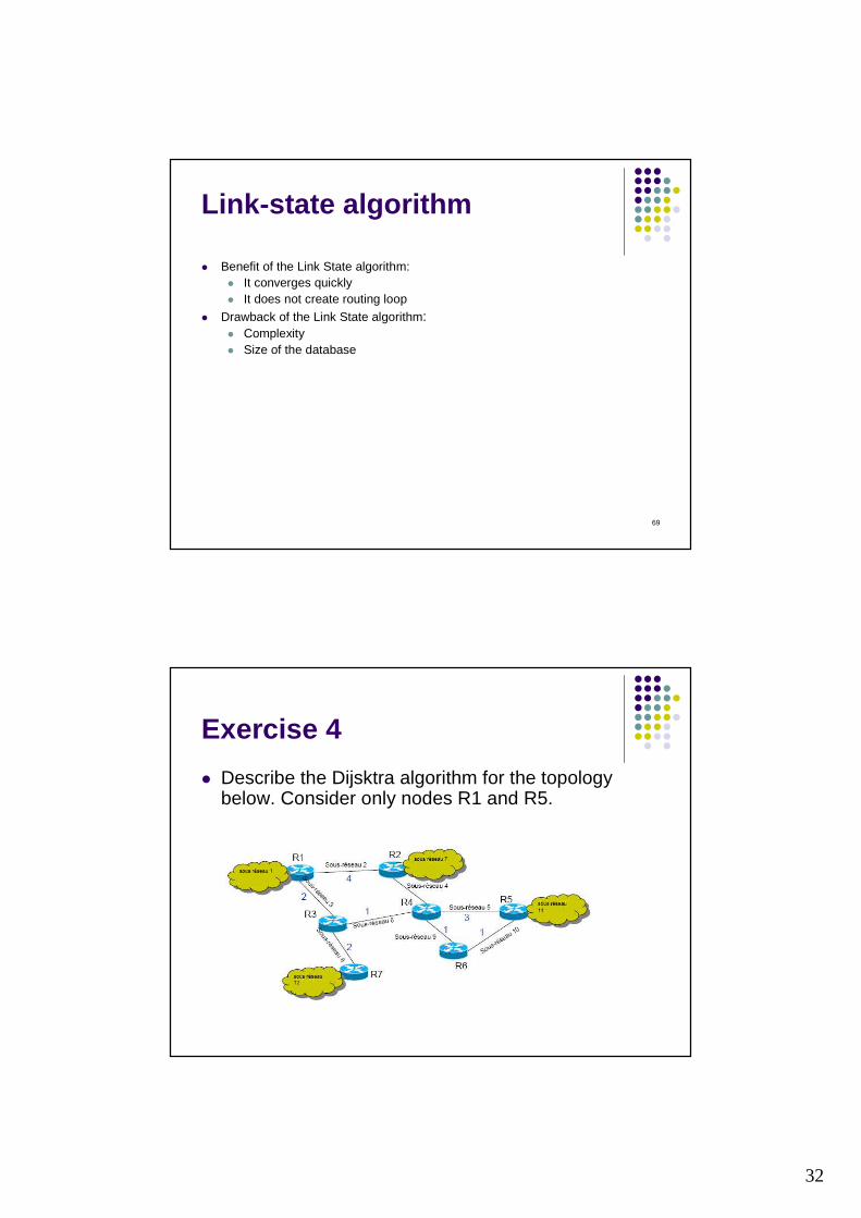
Exercise 4
� Describe the Dijsktra algorithm for the topologybelow. Consider only nodes R1 and R5.
33
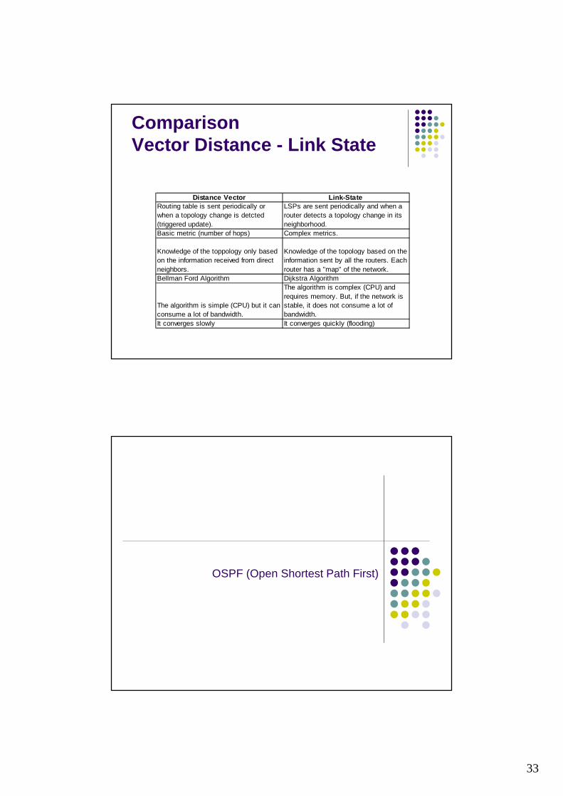
ComparisonVector Distance - Link State
Distance Vector Link-StateRouting table is sent periodically or when a topology change is detcted (triggered update).
LSPs are sent periodically and when a router detects a topology change in its neighborhood.
Basic metric (number of hops) Complex metrics.
Knowledge of the toppology only based on the information received from direct neighbors.
Knowledge of the topology based on the information sent by all the routers. Each router has a "map" of the network.
Bellman Ford Algorithm Dijkstra Algorithm
The algorithm is simple (CPU) but it can consume a lot of bandwidth.
The algorithm is complex (CPU) and requires memory. But, if the network is stable, it does not consume a lot of bandwidth.
It converges slowly It converges quickly (flooding)
OSPF (Open Shortest Path First)
34
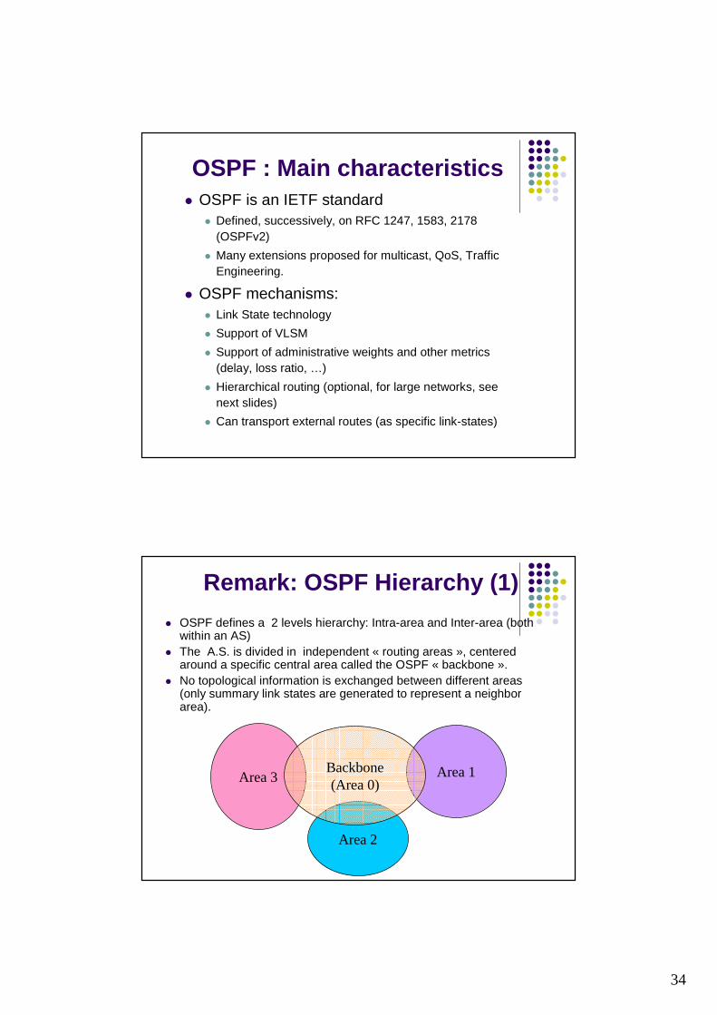
� OSPF is an IETF standard� Defined, successively, on RFC 1247, 1583, 2178
(OSPFv2)
� Many extensions proposed for multicast, QoS, Traffic Engineering.
� OSPF mechanisms:� Link State technology
� Support of VLSM
� Support of administrative weights and other metrics (delay, loss ratio, …)
� Hierarchical routing (optional, for large networks, see next slides)
� Can transport external routes (as specific link-states)
OSPF : Main characteristics
Area 3
Area 2
Area 1
� OSPF defines a 2 levels hierarchy: Intra-area and Inter-area (both within an AS)
� The A.S. is divided in independent « routing areas », centeredaround a specific central area called the OSPF « backbone ».
� No topological information is exchanged between different areas (only summary link states are generated to represent a neighborarea).
Remark: OSPF Hierarchy (1)
Backbone(Area 0)
35
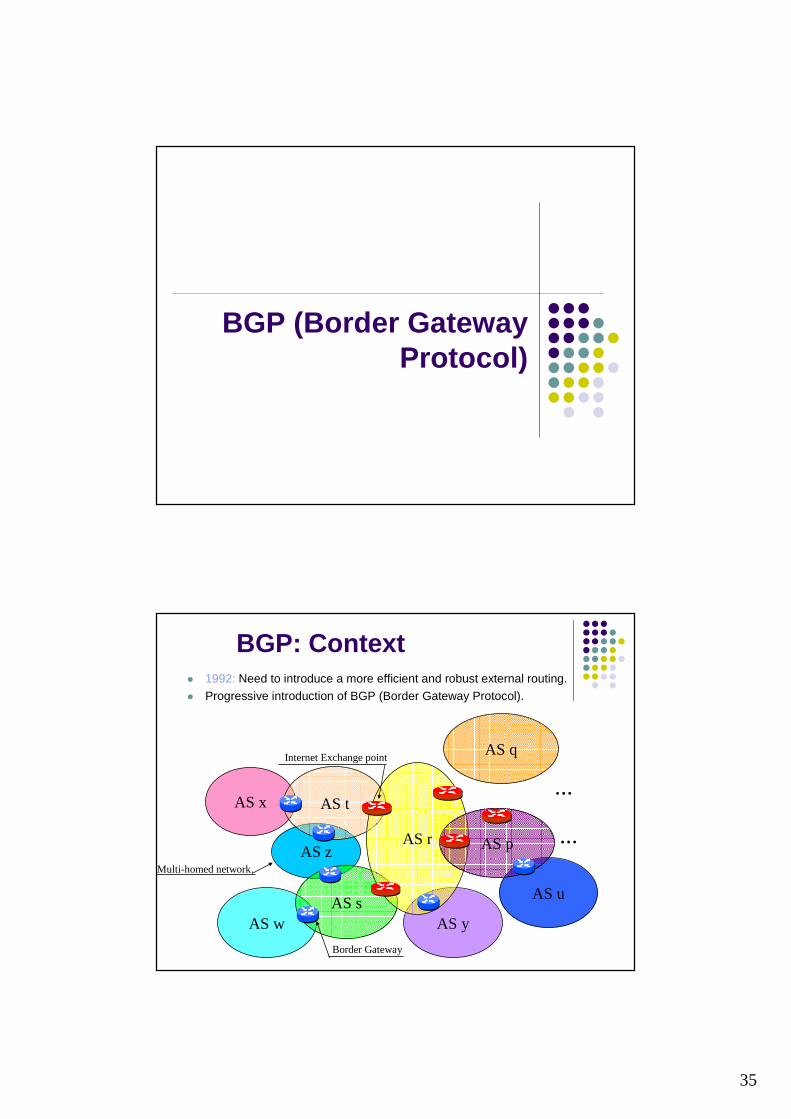
BGP (Border Gateway Protocol)
AS u
AS w
� 1992: Need to introduce a more efficient and robust external routing.
� Progressive introduction of BGP (Border Gateway Protocol).
BGP: Context
AS x
AS z
AS y
AS t
AS s
AS r
Multi-homed network.
Border Gateway
Internet Exchange pointAS q
...
AS p ...
36
BGP: Rationales
� Choice of Routing Technology:� Link State can’t be used for internet wide
graph� Use of hierarchy seems difficult to implement,
in particular for political reasons
� Distance Vector scales…� But has robustness issues that need to be
addressed.� Proposed extensions for robustness:
� Path Vector (see below) for loop avoidance
� Incremental updates (scalability, limitation of overhead)
� Runs on top of TCP (robustness)
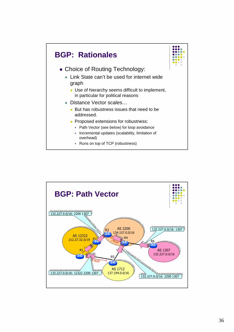
AS 12322212.27.32.0/19 AS 12322
212.27.32.0/19
AS 2200134.157.0.0/16AS 2200
134.157.0.0/16
BGP: Path Vector
AS 1307132.227.0.0/16AS 1307
132.227.0.0/16
AS 1712137.194.0.0/16AS 1712
137.194.0.0/16
e-BGP
i-BGP
132.227.0.0/16: 1307132.227.0.0/16: 1307
R1
R2
R3
R4
R5
R6
132.227.0.0/16: 12322 2200 1307132.227.0.0/16: 12322 2200 1307132.227.0.0/16: 2200 1307132.227.0.0/16: 2200 1307
132.227.0.0/16: 2200 1307132.227.0.0/16: 2200 1307
37
AS 1712137.194.0.0/16AS 1712
137.194.0.0/16
AS 12322212.27.32.0/19 AS 12322
212.27.32.0/19
AS 2200134.157.0.0/16AS 2200
134.157.0.0/16
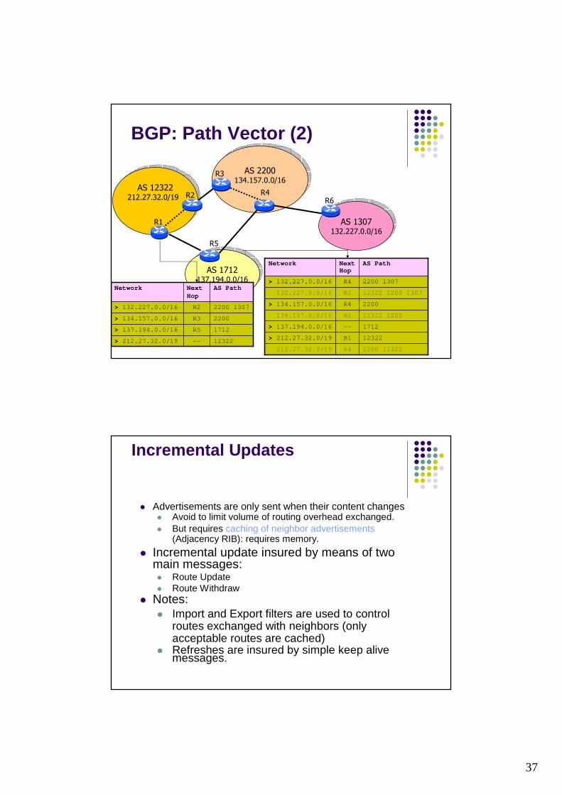
BGP: Path Vector (2)
AS 1307132.227.0.0/16AS 1307
132.227.0.0/16
R1
R2
R3
R4
R5
R6
12322R1> 212.27.32.0/19
2200 12322R4212.27.32.0/19
1712--> 137.194.0.0/16
12322 2200R1134.157.0.0/16
2200R4> 134.157.0.0/16
12322 2200 1307R1132.227.0.0/16
2200 1307R4> 132.227.0.0/16
AS PathNextHop
Network
12322--> 212.27.32.0/19
1712R5> 137.194.0.0/16
2200R3> 134.157.0.0/16
2200 1307R2> 132.227.0.0/16
AS PathNextHop
Network
Incremental Updates
� Advertisements are only sent when their content changes� Avoid to limit volume of routing overhead exchanged.� But requires caching of neighbor advertisements
(Adjacency RIB): requires memory.
� Incremental update insured by means of two main messages: � Route Update � Route Withdraw
� Notes:� Import and Export filters are used to control
routes exchanged with neighbors (only acceptable routes are cached)
� Refreshes are insured by simple keep alive messages.