Embed Size (px)
Citation preview
Advanced routing topics
Tuomas Launiainen
Suboptimal routing
Routing trees
Measurement of routing trees
Adaptive routing
Problems
Fault-tolerant tables
Point-of-failure rerouting
Point-of-failure shortest path rerouting
Correctness
Compact tables
Routing with interwals
Restrictions used:
I Bidirectional Links (BL)
I Connectivity (CN)
I Total Reliability (TR)
I Initial Distinct Values (ID)

Suboptimal routing
I Optimal (shortest path guaranteed) routing is expensive
I Suboptimal routing does not guarantee shortest paths, but isoften sufficient
Routing trees
Routing can be done using a single spanning tree, a routing tree.All messages are passed using only the edges in the routing tree.
I Relatively easy to construct
I Guaranteed delivery
I Guaranteed to use no more messages than the diameter of thetree

Centre-based routing tree
Since messages are delivered with no more than diam(T ) hops in arouting tree T , one logical choise for the routing tree is one rootedat the centre of the graph (a node that has the smallest distanceto the farthest node from it).
Construction:
1. Find the centre of the graph
2. Construct the shortest path spanning tree for that node
The diameter of the spanning tree is bound from above:diam(G ) ≤ diam(PT(c)) ≤ 2diam(G ).
Median-based routing tree
Since a tree has no loops, each edge e = (x , y) of the routing treesplits the tree in two: T [x − y ], and T [y − x ]. This means thatevery message passing from one half to the other must go throughe, the use of which costs θ(e).
If all nodes send the same amount of messages on average, andthe destinations are evenly distributed independent of the sender,the overall average cost of using T for routing is relative to:
∑(x ,y)∈T
|T [x − y ]| |T [y − x ]| θ((x , y))
This is also the sum of all distances between every pair of nodes.

Median-based routing tree (contd.)
If message passing is evenly distributed, the overall cost of arouting tree can be minimized by minimizing the sum of everydistance in the tree. Unfortunately constructing such a tree isdifficult.
A near-optimal solution, a median-based routing tree, is simple toconstruct, however. The median node of a graph is one that hasthe smallest sum of distances to every other node.
The average cost of a median-based routing tree is (claimed to be)no worse than twice the average cost of the cost-minimizingrouting tree.

Minimum-cost routing tree
Another natural choise is the spanning tree that minimizes the sumof costs of it’s edges. It can be constructed with e.g. MegaMerger.

Measurement of routing trees
Examine how much a routing tree stretches the distance betweentwo nodes.
I Strecth factor: the maximum streching between nodes:maxx ,y∈V
dT (x ,y)dG (x ,y)
I Dilation: the maximum length between neighbours in theoriginal graph: max
(x ,y)∈EdT (x , y)
I Edge-stretch factor: maximum stretch of an edge:max
(x ,y)∈E
dT (x ,y)θ((x ,y)) (also called the dilation factor)
I Also average stretch factor and average dilation factor

Adaptive routing
Adaptive routing tries to handle routing in a system where thecosts of edges change.
I When the cost of a link (x , y) changes, both x and y arenotified
I The restriction Total Reliability is replaced with TotalComponent Reliability
I New restriction Cost Change Detection
I A link failure can be described by setting it’s cost to ∞
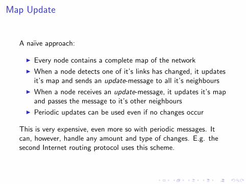
Map Update
A naıve approach:
I Every node contains a complete map of the network
I When a node detects one of it’s links has changed, it updatesit’s map and sends an update-message to all it’s neighbours
I When a node receives an update-message, it updates it’s mapand passes the message to it’s other neighbours
I Periodic updates can be used even if no changes occur
This is very expensive, even more so with periodic messages. Itcan, however, handle any amount and type of changes. E.g. thesecond Internet routing protocol uses this scheme.
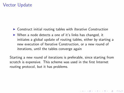
Vector Update
I Construct initial routing tables with Iterative Construction
I When a node detects a one of it’s links has changed, itinitiates a global update of routing tables, either by starting anew execution of Iterative Construction, or a new round ofiterations, until the tables converge again
Starting a new round of iterations is preferable, since starting fromscratch is expensive. This scheme was used in the first Internetrouting protocol, but it has problems.

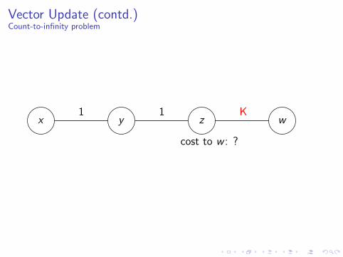
Vector Update (contd.)Count-to-infinity problem
x y z w1 1 1
cost to w : 1
Vector Update (contd.)Count-to-infinity problem
x y z w1 1 K
cost to w : ?

Vector Update (contd.)Count-to-infinity problem
x y z w1 1 K
cost to w : 3

Vector Update (contd.)Count-to-infinity problem
x y z w1 1 K
cost to w : 3cost to w : 4

Oscillation
A problem concerning many approaches is oscillation. It occurswhen the cost of using a link is proportional to the amount oftraffic through it.
x
z
w
y
If x wants to send lots of messages to y , the best path will start tooscillate between z and w .

Fault-tolerant tables
Upholding optimal routing tables in a changing system is veryexpensive. If suboptimal routes are allowed and link failures arelimited to a single link at a time (single-link crash failure),fault-tolerant tables can be used to relay messages with minimalcommunication.

Point-of-failure rerouting
I Each node stores two edge-disjoint paths to each destination.
I Messages are delivered through the shortest path from theirsource to their destination, assuming no link crashes haveoccurred.
I If the message arrives to a node whose link has crashed (pointof failure), it is rerouted to it’s destination via the alternatepath.
Suboptimal service is provided only when a crash occurs, andinformation about crashes does not need to be relayed.
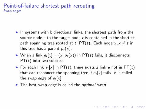
Point-of-failure shortest path reroutingSwap edges
I In systems with bidirectional links, the shortest path from thesource node s to the target node t is contained in the shortestpath spanning tree rooted at t, PT(t). Each node x , x 6= t inthis tree has a parent pt(x).
I When a link et [x ] = (x , pt(x)) in PT(t) fails, it disconnectsPT(t) into two subtrees.
I For each link et [x ] in PT(t), there exists a link e not in PT(t)that can reconnect the spanning tree if et [x ] fails. e is calledthe swap edge of et [x ].
I The best swap edge is called the optimal swap.
Point-of-failure shortest path rerouting (contd.)Routing tables
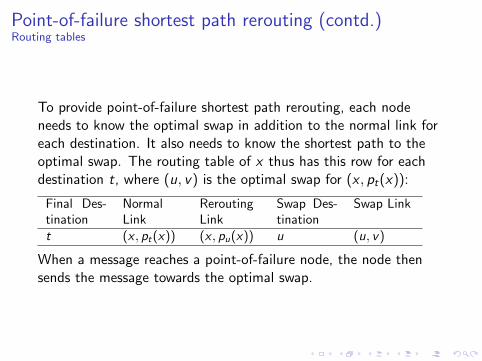
To provide point-of-failure shortest path rerouting, each nodeneeds to know the optimal swap in addition to the normal link foreach destination. It also needs to know the shortest path to theoptimal swap. The routing table of x thus has this row for eachdestination t, where (u, v) is the optimal swap for (x , pt(x)):
Final Des-tination
NormalLink
ReroutingLink
Swap Des-tination
Swap Link
t (x , pt(x)) (x , pu(x)) u (u, v)
When a message reaches a point-of-failure node, the node thensends the message towards the optimal swap.

Point-of-failure shortest path rerouting (contd.)Algorithm (sort of)
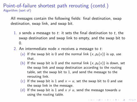
All messages contain the following fields: final destination, swapdestination, swap link, and swap bit.
1. s sends a message to t: it sets the final destination to t, theswap destination and swap link to empty, and the swap bit to0.
2. An intermediate node x receives a message to t:
(a) If the swap bit is 0 and the normal link (x , pt(x)) is up, usethat.
(b) If the swap bit is 0 and the normal link (x , pt(x)) is down, setthe swap link and swap destination according to the routingtable, set the swap bit to 1, and send the message to thererouting link.
(c) If the swap bit is 1 and x = u, set the swap bit to 0 and usethe swap link in the message.
(d) If the swap bit is 1 and x 6= u, send the message towards uusing the routing table.

Point-of-failure shortest path rerouting (contd.)Algorithm (sort of)
All messages contain the following fields: final destination, swapdestination, swap link, and swap bit.
1. s sends a message to t: it sets the final destination to t, theswap destination and swap link to empty, and the swap bit to0.
2. An intermediate node x receives a message to t:
(a) If the swap bit is 0 and the normal link (x , pt(x)) is up, usethat.
(b) If the swap bit is 0 and the normal link (x , pt(x)) is down, setthe swap link and swap destination according to the routingtable, set the swap bit to 1, and send the message to thererouting link.
(c) If the swap bit is 1 and x = u, set the swap bit to 0 and usethe swap link in the message.
(d) If the swap bit is 1 and x 6= u, send the message towards uusing the routing table.

Correctness
Consider this example, where the blue node wants to send amessage to the green node, but just before the message reaches it,the red link before it goes down.
We cannot make any guarantees that a message will arrive to it’sdestination. We can, however, guarantee that if the changes in thesystem stop (for a long enough period), the message will bedelivered through the point-of-failure shortest path.

Compact tables
Routing tables are quite large:
I O(n2 log n) bits each for full routing tables
I O(n log n) bits each, if only destination-link pairs are stored(for each destination t, the routing table of x stores the link(x , pt(x)))
Without special knowledge about node naming and networktopology, this is about as good as we can get, since an entry needsto be made for each destination.
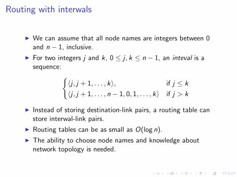
Routing with interwals
I We can assume that all node names are integers between 0and n − 1, inclusive.
I For two integers j and k, 0 ≤ j , k ≤ n − 1, an inteval is asequence:{
〈j , j + 1, . . . , k〉, if j ≤ k
〈j , j + 1, . . . , n − 1, 0, 1, . . . , k〉 if j > k
I Instead of storing destination-link pairs, a routing table canstore interwal-link pairs.
I Routing tables can be as small as O(log n).
I The ability to choose node names and knowledge aboutnetwork topology is needed.

Routing with interwals (contd.)Example
0
7 2
36
1
45
right
The routing table of 0
Link Interwal
left (1, 4) = 〈1, 2, 3, 4〉right (5, 7) = 〈5, 6, 7〉
In sorted and directed rings O(log n) can be achieved.
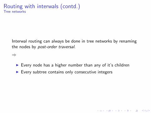
Routing with interwals (contd.)Tree networks
Interwal routing can always be done in tree networks by renamingthe nodes by post-order traversal.
⇒
I Every node has a higher number than any of it’s children
I Every subtree contains only consecutive integers

Routing with interwals (contd.)Tree example
15
0 1
2
3
4 5
6 7
121110
9
14
13
8
An example of a 16-node tree network with nodes named bypost-order traversal.
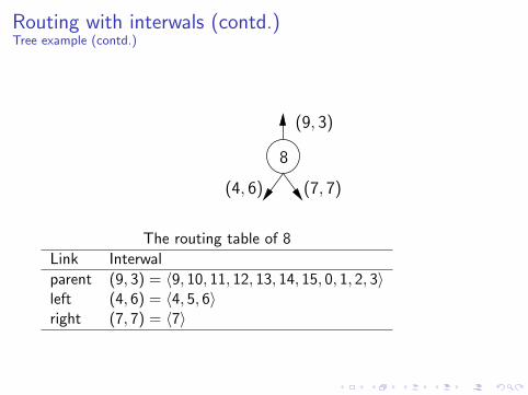
Routing with interwals (contd.)Tree example (contd.)
8
(9, 3)
(7, 7)(4, 6)
The routing table of 8
Link Interwal
parent (9, 3) = 〈9, 10, 11, 12, 13, 14, 15, 0, 1, 2, 3〉left (4, 6) = 〈4, 5, 6〉right (7, 7) = 〈7〉

Routing with interwals (contd.)Globe graph
Interwal routing is not always possible, however. Here is anexample of such a case, called a globe graph:

Suboptimal routing with interwals
If providing shortest path routing is not necessary, for any networka routing tree can be constructed. As already seen, interwalrouting always works in trees.

Recap
I Optimal routing is expensive, but suboptimal, efficient, andoften good enough solutions exist. The primary methodcovered here uses some spanning tree to route traffic.
I Adaptive routing tries to cope with changing costs of links.Optimal solutions are very expensive, but e.g. point-of-failurererouting uses no extra communication after the initialconstruction, and manages single-link crash failures. Messagedelivery cannot be guaranteed while crashes continue tooccur, however.
I Complete routing tables are very large. The only way to getbelow O(n log n) size per table is to use special knowledgeabout the network.