Embed Size (px)
Citation preview

Implied volatility Stochastic volatility Realized volatility The RFSV model Pricing Fitting SPX Forecasting
Rough volatility
Jim Gatheral(joint work with Christian Bayer, Peter Friz,
Thibault Jaisson, Andrew Lesniewski, and Mathieu Rosenbaum)
National School of Development, Peking University,Tuesday November 10, 2015
Implied volatility Stochastic volatility Realized volatility The RFSV model Pricing Fitting SPX Forecasting
Outline of this talk
The volatility surface: Stylized facts
A remarkable monofractal scaling property of historicalvolatility
Fractional Brownian motion (fBm)
The Rough Fractional Stochastic Volatility (RFSV) model
The Rough Bergomi (rBergomi) model
Fits to SPX
Forecasting the variance swap curve

Implied volatility Stochastic volatility Realized volatility The RFSV model Pricing Fitting SPX Forecasting
SPX volatility smiles as of 15-Sep-2005
Figure 1: SVI fit superimposed on smiles.

Implied volatility Stochastic volatility Realized volatility The RFSV model Pricing Fitting SPX Forecasting
The SPX volatility surface as of 15-Sep-2005
Figure 2: The SPX volatility surface as of 15-Sep-2005 (Figure 3.2 ofThe Volatility Surface).

Implied volatility Stochastic volatility Realized volatility The RFSV model Pricing Fitting SPX Forecasting
Interpreting the smile
We could say that the volatility smile (at least in equitymarkets) reflects two basic observations:
Volatility tends to increase when the underlying price falls,
hence the negative skew.
We don’t know in advance what realized volatility will be,
hence implied volatility is increasing in the wings.
It’s implicit in the above that more or less any model that isconsistent with these two observations will be able to fit onegiven smile.
Fitting two or more smiles simultaneously is much harder.
Heston for example fits a maximum of two smilessimultaneously.SABR can only fit one smile at a time.
Implied volatility Stochastic volatility Realized volatility The RFSV model Pricing Fitting SPX Forecasting
Term structure of at-the-money skew
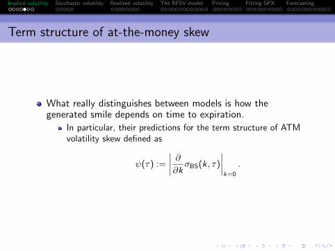
What really distinguishes between models is how thegenerated smile depends on time to expiration.
In particular, their predictions for the term structure of ATMvolatility skew defined as
ψ(τ) :=
∣∣∣∣ ∂∂k σBS(k , τ)
∣∣∣∣k=0
.

Implied volatility Stochastic volatility Realized volatility The RFSV model Pricing Fitting SPX Forecasting
Term structure of SPX ATM skew as of 15-Sep-2005
Figure 3: Term structure of ATM skew as of 15-Sep-2005, with powerlaw fit τ−0.44 superimposed in red.

Implied volatility Stochastic volatility Realized volatility The RFSV model Pricing Fitting SPX Forecasting
Stylized facts
Although the levels and orientations of the volatility surfaceschange over time, their rough shape stays very much thesame.
It’s then natural to look for a time-homogeneous model.
The term structure of ATM volatility skew
ψ(τ) ∼ 1
τα
with α ∈ (0.3, 0.5).

Implied volatility Stochastic volatility Realized volatility The RFSV model Pricing Fitting SPX Forecasting
Motivation for Rough Volatility I: Better fitting stochasticvolatility models
Conventional stochastic volatility models generate volatilitysurfaces that are inconsistent with the observed volatilitysurface.
In stochastic volatility models, the ATM volatility skew isconstant for short dates and inversely proportional to T forlong dates.Empirically, we find that the term structure of ATM skew isproportional to 1/Tα for some 0 < α < 1/2 over a very widerange of expirations.
The conventional solution is to introduce more volatilityfactors, as for example in the DMR and Bergomi models.
One could imagine the power-law decay of ATM skew to bethe result of adding (or averaging) many sub-processes, eachof which is characteristic of a trading style with a particulartime horizon.

Implied volatility Stochastic volatility Realized volatility The RFSV model Pricing Fitting SPX Forecasting
Bergomi Guyon
Define the forward variance curve ξt(u) = E [vu| Ft ].
According to [Bergomi and Guyon], in the context of avariance curve model, implied volatility may be expanded as
σBS(k ,T ) = σ0(T ) +
√w
T
1
2w2C x ξ k + O(η2) (1)
where η is volatility of volatility, w =∫ T
0 ξ0(s) ds is totalvariance to expiration T , and
C x ξ =
∫ T
0dt
∫ T
tdu
E [dxt dξt(u)]
dt. (2)
Thus, given a stochastic model, defined in terms of an SDE,we can easily (at least in principle) compute this smileapproximation.
Implied volatility Stochastic volatility Realized volatility The RFSV model Pricing Fitting SPX Forecasting
The Bergomi model
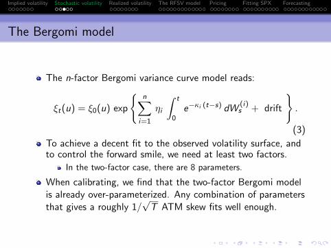
The n-factor Bergomi variance curve model reads:
ξt(u) = ξ0(u) exp
{n∑
i=1
ηi
∫ t
0e−κi (t−s) dW
(i)s + drift
}.
(3)
To achieve a decent fit to the observed volatility surface, andto control the forward smile, we need at least two factors.
In the two-factor case, there are 8 parameters.
When calibrating, we find that the two-factor Bergomi modelis already over-parameterized. Any combination of parametersthat gives a roughly 1/
√T ATM skew fits well enough.

Implied volatility Stochastic volatility Realized volatility The RFSV model Pricing Fitting SPX Forecasting
ATM skew in the Bergomi model
The Bergomi model generates a term structure of volatilityskew ψ(τ) that is something like
ψ(τ) =∑
i
1
κi τ
{1− 1− e−κi τ
κi τ
}.
This functional form is related to the term structure of theautocorrelation function.Which is in turn driven by the exponential kernel in theexponent in (3).
The observed ψ(τ) ∼ τ−α for some α.
It’s tempting to replace the exponential kernels in (3) with apower-law kernel.

Implied volatility Stochastic volatility Realized volatility The RFSV model Pricing Fitting SPX Forecasting
Tinkering with the Bergomi model
This would give a model of the form
ξt(u) = ξ0(u) exp
{η
∫ t
0
dWs
(t − s)γ+ drift
}which looks similar to
ξt(u) = ξ0(u) exp{ηWH
t + drift}
where WHt is fractional Brownian motion.

Implied volatility Stochastic volatility Realized volatility The RFSV model Pricing Fitting SPX Forecasting
Motivation for Rough Volatility II: Power-law scaling of thevolatility process
The Oxford-Man Institute of Quantitative Finance makeshistorical realized variance (RV) estimates freely available athttp://realized.oxford-man.ox.ac.uk. These estimatesare updated daily.
Using daily RV estimates as proxies for instantaneous variance,we may investigate the time series properties of vt empirically.

Implied volatility Stochastic volatility Realized volatility The RFSV model Pricing Fitting SPX Forecasting
SPX realized variance from 2000 to 2014
Figure 4: KRV estimates of SPX realized variance from 2000 to 2014.

Implied volatility Stochastic volatility Realized volatility The RFSV model Pricing Fitting SPX Forecasting
The smoothness of the volatility process
For q ≥ 0, we define the qth sample moment of differences oflog-volatility at a given lag ∆1:
m(q,∆) = 〈|log σt+∆ − log σt |q〉
For example
m(2,∆) = 〈(log σt+∆ − log σt)2〉
is just the sample variance of differences in log-volatility at thelag ∆.
1〈·〉 denotes the sample average.

Implied volatility Stochastic volatility Realized volatility The RFSV model Pricing Fitting SPX Forecasting
Scaling of m(q,∆) with lag ∆
Figure 5: logm(q,∆) as a function of log ∆, SPX.

Implied volatility Stochastic volatility Realized volatility The RFSV model Pricing Fitting SPX Forecasting
Monofractal scaling result
From the log-log plot Figure 5, we see that for each q,m(q,∆) ∝ ∆ζq .
Furthermore, we find the monofractal scaling relationship
ζq = q H
with H ≈ 0.14.
Note however that H does vary over time, in a narrow range.Note also that our estimate of H is biased high because weproxied instantaneous variance vt with its average over each
day 1T
∫ T
0vt dt, where T is one day.

Implied volatility Stochastic volatility Realized volatility The RFSV model Pricing Fitting SPX Forecasting
Distributions of (log σt+∆ − log σt) for various lags ∆
Figure 6: Histograms of (log σt+∆ − log σt) for various lags ∆; normalfit in red; ∆ = 1 normal fit scaled by ∆0.14 in blue.

Implied volatility Stochastic volatility Realized volatility The RFSV model Pricing Fitting SPX Forecasting
Estimated H for all indices
Repeating this analysis for all 21 indices in the Oxford-Man datasetyields:
Index ζ0.5/0.5 ζ1 ζ1.5/1.5 ζ2/2 ζ3/3SPX2.rv 0.128 0.126 0.125 0.124 0.124FTSE2.rv 0.132 0.132 0.132 0.131 0.127N2252.rv 0.131 0.131 0.132 0.132 0.133GDAXI2.rv 0.141 0.139 0.138 0.136 0.132RUT2.rv 0.117 0.115 0.113 0.111 0.108AORD2.rv 0.072 0.073 0.074 0.075 0.077DJI2.rv 0.117 0.116 0.115 0.114 0.113IXIC2.rv 0.131 0.133 0.134 0.135 0.137FCHI2.rv 0.143 0.143 0.142 0.141 0.138HSI2.rv 0.079 0.079 0.079 0.080 0.082KS11.rv 0.133 0.133 0.134 0.134 0.132AEX.rv 0.145 0.147 0.149 0.149 0.149SSMI.rv 0.149 0.153 0.156 0.158 0.158IBEX2.rv 0.138 0.138 0.137 0.136 0.133NSEI.rv 0.119 0.117 0.114 0.111 0.102MXX.rv 0.077 0.077 0.076 0.075 0.071BVSP.rv 0.118 0.118 0.119 0.120 0.120GSPTSE.rv 0.106 0.104 0.103 0.102 0.101STOXX50E.rv 0.139 0.135 0.130 0.123 0.101FTSTI.rv 0.111 0.112 0.113 0.113 0.112FTSEMIB.rv 0.130 0.132 0.133 0.134 0.134
Table 1: Estimates of ζq for all indices in the Oxford-Man dataset.

Implied volatility Stochastic volatility Realized volatility The RFSV model Pricing Fitting SPX Forecasting
Universality?
[Gatheral, Jaisson and Rosenbaum] compute daily realizedvariance estimates over one hour windows for DAX and Bundfutures contracts, finding similar scaling relationships.
We have also checked that Gold and Crude Oil futures scalesimilarly.
Although the increments (log σt+∆ − log σt) seem to be fattertailed than Gaussian.

Implied volatility Stochastic volatility Realized volatility The RFSV model Pricing Fitting SPX Forecasting
A natural model of realized volatility
Distributions of differences in the log of realized volatility areclose to Gaussian.
This motivates us to model σt as a lognormal random variable.
Moreover, the scaling property of variance of RV differencessuggests the model:
log σt+∆ − log σt = ν(WH
t+∆ −WHt
)(4)
where WH is fractional Brownian motion.
In [Gatheral, Jaisson and Rosenbaum], we refer to a stationaryversion of (4) as the RFSV (for Rough Fractional StochasticVolatility) model.

Implied volatility Stochastic volatility Realized volatility The RFSV model Pricing Fitting SPX Forecasting
Fractional Brownian motion (fBm)
Fractional Brownian motion (fBm) {WHt ; t ∈ R} is the unique
Gaussian process with mean zero and autocovariance function
E[WH
t WHs
]=
1
2
{|t|2 H + |s|2 H − |t − s|2 H
}where H ∈ (0, 1) is called the Hurst index or parameter.
In particular, when H = 1/2, fBm is just Brownian motion.
If H > 1/2, increments are positively correlated.If H < 1/2, increments are negatively correlated.
Implied volatility Stochastic volatility Realized volatility The RFSV model Pricing Fitting SPX Forecasting
Representations of fBm
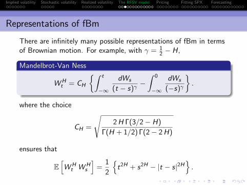
There are infinitely many possible representations of fBm in termsof Brownian motion. For example, with γ = 1
2 − H,
Mandelbrot-Van Ness
WHt = CH
{∫ t
−∞
dWs
(t − s)γ−∫ 0
−∞
dWs
(−s)γ
}.
where the choice
CH =
√2H Γ(3/2− H)
Γ(H + 1/2) Γ(2− 2H)
ensures that
E[WH
t WHs
]=
1
2
{t2H + s2H − |t − s|2H
}.

Implied volatility Stochastic volatility Realized volatility The RFSV model Pricing Fitting SPX Forecasting
Comte and Renault: FSV model
[Comte and Renault] were perhaps the first to model volatilityusing fractional Brownian motion.
In their fractional stochastic volatility (FSV) model,
dSt
St= σt dZt
d log σt = −α (log σt − θ) dt + γ dWHt (5)
with
WHt =
∫ t
0
(t − s)H−1/2
Γ(H + 1/2)dWs , 1/2 ≤ H < 1
and E [dWt dZt ] = ρ dt.
The FSV model is a generalization of the Hull-Whitestochastic volatility model.

Implied volatility Stochastic volatility Realized volatility The RFSV model Pricing Fitting SPX Forecasting
RFSV and FSV
The model (4):
log σt+∆ − log σt = ν(WH
t+∆ −WHt
)(6)
is not stationary.
Stationarity is desirable both for mathematical tractability andalso to ensure reasonableness of the model at very large times.
The RFSV model (the stationary version of (4)) is formallyidentical to the FSV model. Except that
H < 1/2 in RFSV vs H > 1/2 in FSV.αT � 1 in RFSV vs αT ∼ 1 in FSV
where T is a typical timescale of interest.

Implied volatility Stochastic volatility Realized volatility The RFSV model Pricing Fitting SPX Forecasting
FSV and long memory
Why did [Comte and Renault] choose H > 1/2?Because it has been a widely-accepted stylized fact that thevolatility time series exhibits long memory.
In this technical sense, long memory means that theautocorrelation function of volatility decays as a power-law.One of the influential papers that established this was[Andersen et al.] which estimated the degree d of fractionalintegration from daily realized variance data for the 30 DJIAstocks.
Using the GPH estimator, they found d around 0.35 whichimplies that the ACF ρ(τ) ∼ τ 2 d−1 = τ−0.3 as τ →∞.
But every statistical estimator assumes the validity of someunderlying model!
In the RFSV model,
ρ(∆) ∼ exp
{−η
2
2∆2 H
}.
Implied volatility Stochastic volatility Realized volatility The RFSV model Pricing Fitting SPX Forecasting
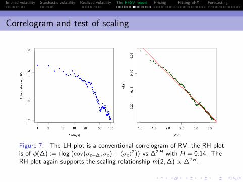
Correlogram and test of scaling
Figure 7: The LH plot is a conventional correlogram of RV; the RH plotis of φ(∆) := 〈log
(cov(σt+∆, σt) + 〈σt〉2
)〉 vs ∆2 H with H = 0.14. The
RH plot again supports the scaling relationship m(2,∆) ∝ ∆2 H .

Implied volatility Stochastic volatility Realized volatility The RFSV model Pricing Fitting SPX Forecasting
Model vs empirical autocorrelation functions
Figure 8: Here we superimpose the RFSV functional form
ρ(∆) ∼ exp{−η
2
2 ∆2 H}
(in red) on the empirical curve (in blue).

Implied volatility Stochastic volatility Realized volatility The RFSV model Pricing Fitting SPX Forecasting
Volatility is not long memory
It’s clear from Figures 7 and 8 that volatility is not longmemory.
Moreover, the RFSV model reproduces the observedautocorrelation function very closely.
[Gatheral, Jaisson and Rosenbaum] further simulate volatilityin the RFSV model and apply standard estimators to thesimulated data.
Real data and simulated data generate very similar plots andsimilar estimates of the long memory parameter to thosefound in the prior literature.
The RSFV model does not have the long memory property.
Classical estimation procedures seem to identify spurious longmemory of volatility.

Implied volatility Stochastic volatility Realized volatility The RFSV model Pricing Fitting SPX Forecasting
Incompatibility of FSV with realized variance (RV) data
In Figure 9, we demonstrate graphically that long memoryvolatility models such as FSV with H > 1/2 are notcompatible with the RV data.
In the FSV model, the autocorrelation functionρ(∆) ∝ ∆2 H−2. Then, for long memory, we must have1/2 < H < 1.
For ∆� 1/α, stationarity kicks in and m(2,∆) tends to aconstant as ∆→∞.For ∆� 1/α, mean reversion is not significant andm(2,∆) ∝ ∆2 H .

Implied volatility Stochastic volatility Realized volatility The RFSV model Pricing Fitting SPX Forecasting
Incompatibility of FSV with RV data
Figure 9: Black points are empirical estimates of m(2,∆); the blue lineis the FSV model with α = 0.5 and H = 0.53; the orange line is theRFSV model with α = 0 and H = 0.14.

Implied volatility Stochastic volatility Realized volatility The RFSV model Pricing Fitting SPX Forecasting
Does simulated RSFV data look real?
Figure 10: Volatility of SPX (above) and of the RFSV model (below).

Implied volatility Stochastic volatility Realized volatility The RFSV model Pricing Fitting SPX Forecasting
Remarks on the comparison
The simulated and actual graphs look very alike.
Persistent periods of high volatility alternate with low volatilityperiods.
H ∼ 0.1 generates very rough looking sample paths(compared with H = 1/2 for Brownian motion).
Hence rough volatility.
On closer inspection, we observe fractal-type behavior.
The graph of volatility over a small time period looks like thesame graph over a much longer time period.
This feature of volatility has been investigated both empiricallyand theoretically in, for example, [Bacry and Muzy].
In particular, their Multifractal Random Walk (MRW) isrelated to a limiting case of the RSFV model as H → 0.

Implied volatility Stochastic volatility Realized volatility The RFSV model Pricing Fitting SPX Forecasting
Pricing under rough volatility
The foregoing behavior suggest the following model for volatilityunder the real (or historical or physical) measure P:
log σt = νWHt .
Let γ = 12 − H. We choose the Mandelbrot-Van Ness
representation of fractional Brownian motion WH as follows:
WHt = CH
{∫ t
−∞
dWPs
(t − s)γ−∫ 0
−∞
dWPs
(−s)γ
}where the choice
CH =
√2H Γ(3/2− H)
Γ(H + 1/2) Γ(2− 2H)
ensures that
E[WH
t WHs
]=
1
2
{t2H + s2H − |t − s|2H
}.

Implied volatility Stochastic volatility Realized volatility The RFSV model Pricing Fitting SPX Forecasting
Pricing under rough volatility
Then
log vu − log vt
= ν CH
{∫ u
t
1
(u − s)γdWP
s +
∫ t
−∞
[1
(u − s)γ− 1
(t − s)γ
]dWP
s
}=: 2 ν CH [Mt(u) + Zt(u)] . (7)
Note that EP [Mt(u)| Ft ] = 0 and Zt(u) is Ft-measurable.
To price options, it would seem that we would need to knowFt , the entire history of the Brownian motion Ws for s < t!
Implied volatility Stochastic volatility Realized volatility The RFSV model Pricing Fitting SPX Forecasting
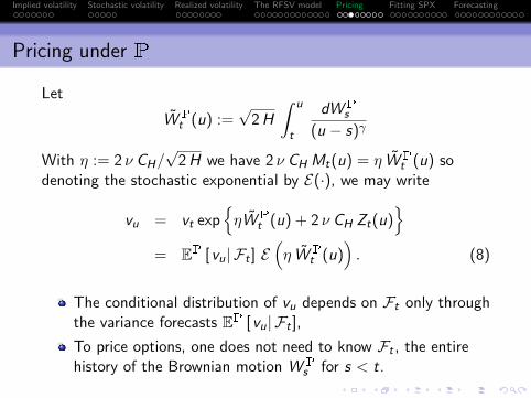
Pricing under P
Let
WPt (u) :=
√2H
∫ u
t
dWPs
(u − s)γ
With η := 2 ν CH/√
2H we have 2 ν CH Mt(u) = η WPt (u) so
denoting the stochastic exponential by E(·), we may write
vu = vt exp{ηWP
t (u) + 2 ν CH Zt(u)}
= EP [vu| Ft ] E(η WP
t (u)). (8)
The conditional distribution of vu depends on Ft only throughthe variance forecasts EP [vu| Ft ],
To price options, one does not need to know Ft , the entirehistory of the Brownian motion WP
s for s < t.

Implied volatility Stochastic volatility Realized volatility The RFSV model Pricing Fitting SPX Forecasting
Pricing under Q
Our model under P reads:
vu = EP [vu| Ft ] E(η WP
t (u)). (9)
Consider some general change of measure
dWPs = dWQ
s + λs ds,
where {λs : s > t} has a natural interpretation as the price ofvolatility risk. We may then rewrite (9) as
vu = EP [vu| Ft ] E(η WQ
t (u))
exp
{η√
2H
∫ u
t
λs
(u − s)γds
}.
Although the conditional distribution of vu under P islognormal, it will not be lognormal in general under Q.
The upward sloping smile in VIX options means λs cannot bedeterministic in this picture.

Implied volatility Stochastic volatility Realized volatility The RFSV model Pricing Fitting SPX Forecasting
The rough Bergomi (rBergomi) model
Let’s nevertheless consider the simplest change of measure
dWPs = dWQ
s + λ(s) ds,
where λ(s) is a deterministic function of s. Then from (38), wewould have
vu = EP [vu| Ft ] E(η WQ
t (u))
exp
{η√
2H
∫ u
t
1
(u − s)γλ(s) ds
}= ξt(u) E
(η WQ
t (u))
(10)
where the forward variances ξt(u) = EQ [vu| Ft ] are (at least inprinciple) tradable and observed in the market.
ξt(u) is the product of two terms:EP [vu| Ft ] which depends on the historical path {Ws , s < t}of the Brownian motiona term which depends on the price of risk λ(s).

Implied volatility Stochastic volatility Realized volatility The RFSV model Pricing Fitting SPX Forecasting
Features of the rough Bergomi model
The rBergomi model is a non-Markovian generalization of theBergomi model:
E [vu| Ft ] 6= E[vu|vt ].
The rBergomi model is Markovian in the (infinite-dimensional)state vector EQ [vu| Ft ] = ξt(u).
We have achieved our aim of replacing the exponential kernelsin the Bergomi model (3) with a power-law kernel.
We may therefore expect that the rBergomi model willgenerate a realistic term structure of ATM volatility skew.

Implied volatility Stochastic volatility Realized volatility The RFSV model Pricing Fitting SPX Forecasting
The stock price process
The observed anticorrelation between price moves andvolatility moves may be modeled naturally by anticorrelatingthe Brownian motion W that drives the volatility process withthe Brownian motion driving the price process.
ThusdSt
St=√vt dZt
withdZt = ρ dWt +
√1− ρ2 dW⊥
t
where ρ is the correlation between volatility moves and pricemoves.

Implied volatility Stochastic volatility Realized volatility The RFSV model Pricing Fitting SPX Forecasting
Simulation of the rBergomi model
We simulate the rBergomi model as follows:
Construct the joint covariance matrix for the Volterra processW and the Brownian motion Z and compute its Choleskydecomposition.
For each time, generate iid normal random vectors andmultiply them by the lower-triangular matrix obtained by theCholesky decomposition to get a m × 2 n matrix of paths ofW and Z with the correct joint marginals.
With these paths held in memory, we may evaluate theexpectation under Q of any payoff of interest.
This procedure is very slow!
Speeding up the simulation is work in progress.

Implied volatility Stochastic volatility Realized volatility The RFSV model Pricing Fitting SPX Forecasting
Guessing rBergomi model parameters
The rBergomi model has only three parameters: H, η and ρ.
If we had a fast simulation, we could just iterate on theseparameters to find the best fit to observed option prices. Butwe don’t.
However, the model parameters H, η and ρ have very directinterpretations:
H controls the decay of ATM skew ψ(τ) for very shortexpirationsThe product ρ η sets the level of the ATM skew for longerexpirations.Keeping ρ η constant but decreasing ρ (so as to make it morenegative) pushes the minimum of each smile towards higherstrikes.
So we can guess parameters in practice.

Implied volatility Stochastic volatility Realized volatility The RFSV model Pricing Fitting SPX Forecasting
Parameter estimation from historical data
Both the roughness parameter (or Hurst parameter) H and thevolatility of volatility η should be the same under P and Q.
Earlier, using the Oxford-Man realized variance dataset, weestimated the Hurst parameter Heff ≈ 0.14 and volatility ofvolatility νeff ≈ 0.3.
However, we not observe the instantaneous volatility σt , only1δ
∫ δ0 σ
2t dt where δ is roughly 3/4 of a whole day from close
to close.
Using Appendix C of [Gatheral, Jaisson and Rosenbaum], werescale finding H ≈ 0.05 and ν ≈ 1.7.
Also, recall that
η = 2 νCH√2H
= 2 ν
√Γ(3/2− H)
Γ(H + 1/2) Γ(2− 2H)
which yields the estimate η ≈ 2.5.

Implied volatility Stochastic volatility Realized volatility The RFSV model Pricing Fitting SPX Forecasting
SPX smiles in the rBergomi model
In Figures 11 and 12, we show how well a rBergomi modelsimulation with guessed parameters fits the SPX optionmarket as of February 4, 2010, a day when the ATM volatilityterm structure happened to be pretty flat.
rBergomi parameters were: H = 0.07, η = 1.9, ρ = −0.9.
Only three parameters to get a very good fit to the whole SPXvolatility surface!

Implied volatility Stochastic volatility Realized volatility The RFSV model Pricing Fitting SPX Forecasting
rBergomi fits to SPX smiles as of 04-Feb-2010
Figure 11: Red and blue points represent bid and offer SPX impliedvolatilities; orange smiles are from the rBergomi simulation.

Implied volatility Stochastic volatility Realized volatility The RFSV model Pricing Fitting SPX Forecasting
Shortest dated smile as of February 4, 2010
Figure 12: Red and blue points represent bid and offer SPX impliedvolatilities; orange smile is from the rBergomi simulation.

Implied volatility Stochastic volatility Realized volatility The RFSV model Pricing Fitting SPX Forecasting
ATM volatilities and skews
In Figures 13 and 14, we see just how well the rBergomi model canmatch empirical skews and vols. Recall also that the parameterswe used are just guesses!

Implied volatility Stochastic volatility Realized volatility The RFSV model Pricing Fitting SPX Forecasting
Term structure of ATM skew as of February 4, 2010
Figure 13: Blue points are empirical skews; the red line is from therBergomi simulation.

Implied volatility Stochastic volatility Realized volatility The RFSV model Pricing Fitting SPX Forecasting
Term structure of ATM vol as of February 4, 2010
Figure 14: Blue points are empirical ATM volatilities; the red line isfrom the rBergomi simulation.

Implied volatility Stochastic volatility Realized volatility The RFSV model Pricing Fitting SPX Forecasting
Another date
Now we take a look at another date: August 14, 2013, twodays before the last expiration date in our dataset.
Options set at the open of August 16, 2013 so only onetrading day left.
Note in particular that the extreme short-dated smile is wellreproduced by the rBergomi model.
There is no need to add jumps!

Implied volatility Stochastic volatility Realized volatility The RFSV model Pricing Fitting SPX Forecasting
SPX smiles as of August 14, 2013
Figure 15: Red and blue points represent bid and offer SPX impliedvolatilities; orange smiles are from the rBergomi simulation.
Implied volatility Stochastic volatility Realized volatility The RFSV model Pricing Fitting SPX Forecasting
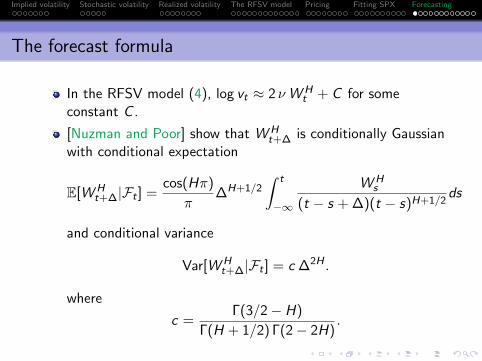
The forecast formula
In the RFSV model (4), log vt ≈ 2 νWHt + C for some
constant C .
[Nuzman and Poor] show that WHt+∆ is conditionally Gaussian
with conditional expectation
E[WHt+∆|Ft ] =
cos(Hπ)
π∆H+1/2
∫ t
−∞
WHs
(t − s + ∆)(t − s)H+1/2ds
and conditional variance
Var[WHt+∆|Ft ] = c ∆2H .
where
c =Γ(3/2− H)
Γ(H + 1/2) Γ(2− 2H).

Implied volatility Stochastic volatility Realized volatility The RFSV model Pricing Fitting SPX Forecasting
The forecast formula
Thus, we obtain
Variance forecast formula
EP [vt+∆| Ft ] = exp{EP [ log(vt+∆)| Ft ] + 2 c ν2∆2 H
}(11)
where
EP [ log vt+∆| Ft ]
=cos(Hπ)
π∆H+1/2
∫ t
−∞
log vs
(t − s + ∆)(t − s)H+1/2ds.
Implied volatility Stochastic volatility Realized volatility The RFSV model Pricing Fitting SPX Forecasting
Forecasting the variance swap curve
For each of 2,658 days from Jan 27, 2003 to August 31, 2013:
We compute proxy variance swaps from closing prices of SPXoptions sourced from OptionMetrics(www.optionmetrics.com) via WRDS.
We form the forecasts EP [vu| Ft ] using (11) with 500 lags ofSPX RV data sourced from The Oxford-Man Institute ofQuantitative Finance(http://realized.oxford-man.ox.ac.uk).
We note that the actual variance swap curve is a factor (ofroughly 1.4) higher than the forecast, which we may attributeto overnight movements of the index.Forecasts must therefore be rescaled to obtain close-to-closerealized variance forecasts.

Implied volatility Stochastic volatility Realized volatility The RFSV model Pricing Fitting SPX Forecasting
The RV scaling factor
Figure 16: The LH plot shows actual (proxy) 3-month variance swapquotes in blue vs forecast in red (with no scaling factor). The RH plotshows the ratio between 3-month actual variance swap quotes and3-month forecasts.
Implied volatility Stochastic volatility Realized volatility The RFSV model Pricing Fitting SPX Forecasting
The Lehman weekend
Empirically, it seems that the variance curve is a simplescaling factor times the forecast, but that this scaling factor istime-varying.
Recall that as of the close on Friday September 12, 2008, itwas widely believed that Lehman Brothers would be rescuedover the weekend. By Monday morning, we knew thatLehman had failed.
In Figure 17, we see that variance swap curves just before andjust after the collapse of Lehman are just rescaled versions ofthe RFSV forecast curves.

Implied volatility Stochastic volatility Realized volatility The RFSV model Pricing Fitting SPX Forecasting
Actual vs predicted over the Lehman weekend
Figure 17: SPX variance swap curves as of September 12, 2008 (red)and September 15, 2008 (blue). The dashed curves are RFSV modelforecasts rescaled by the 3-month ratio (1.29) as of the Friday close.

Implied volatility Stochastic volatility Realized volatility The RFSV model Pricing Fitting SPX Forecasting
Remarks
We note that
The actual variance swaps curves are very close to theforecast curves, up to a scaling factor.
We are able to explain the change in the variance swap curvewith only one extra observation: daily variance over thetrading day on Monday 15-Sep-2008.
The SPX options market appears to be backward-looking in avery sophisticated way.

Implied volatility Stochastic volatility Realized volatility The RFSV model Pricing Fitting SPX Forecasting
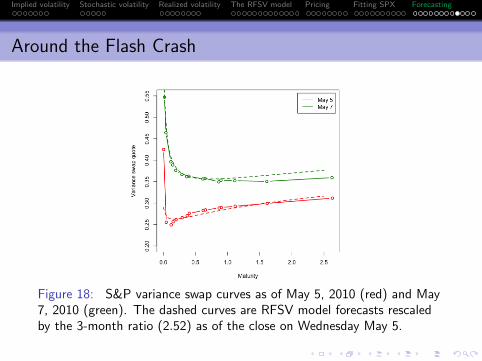
The Flash Crash
The so-called Flash Crash of Thursday May 6, 2010 causedintraday realized variance to be much higher than normal.
In Figure 18, we plot the actual variance swap curves as of theWednesday and Friday market closes together with forecastcurves rescaled by the 3-month ratio as of the close onWednesday May 5 (which was 2.52).
We see that the actual variance curve as of the close onFriday is consistent with a forecast from the time series ofrealized variance that includes the anomalous price action ofThursday May 6.
In Figure 19 we see that the actual variance swap curve onMonday, May 10 is consistent with a forecast that excludesthe Flash Crash.
Volatility traders realized that the Flash Crash should notinfluence future realized variance projections.
Implied volatility Stochastic volatility Realized volatility The RFSV model Pricing Fitting SPX Forecasting
Around the Flash Crash
Figure 18: S&P variance swap curves as of May 5, 2010 (red) and May7, 2010 (green). The dashed curves are RFSV model forecasts rescaledby the 3-month ratio (2.52) as of the close on Wednesday May 5.

Implied volatility Stochastic volatility Realized volatility The RFSV model Pricing Fitting SPX Forecasting
The weekend after the Flash Crash
Figure 19: LH plot: The May 10 actual curve is inconsistent with aforecast that includes the Flash Crash. RH plot: The May 10 actualcurve is consistent with a forecast that excludes the Flash Crash.

Implied volatility Stochastic volatility Realized volatility The RFSV model Pricing Fitting SPX Forecasting
Summary
We uncovered a remarkable monofractal scaling relationship inhistorical volatility.
This leads to a natural non-Markovian stochastic volatilitymodel under P.
The simplest specification of dQdP gives a non-Markovian
generalization of the Bergomi model.
The history of the Brownian motion {Ws , s < t} required forpricing is encoded in the forward variance curve, which isobserved in the market.
This model fits the observed volatility surface surprisingly wellwith very few parameters.
For perhaps the first time, we have a simple consistent modelof historical and implied volatility.

Implied volatility Stochastic volatility Realized volatility The RFSV model Pricing Fitting SPX Forecasting
References
Torben G Andersen, Tim Bollerslev, Francis X Diebold, and Heiko Ebens, The distribution of realized stock
return volatility, Journal of Financial Economics 61 (1) 43–76 (2001).
Christian Bayer, Peter Friz and Jim Gatheral, Pricing under rough volatility, Quantitative Finance,
forthcoming. Available at SSRN 2554754, (2015).
Emmanuel Bacry and Jean-Francois Muzy, Log-infinitely divisible multifractal processes, Communications in
Mathematical Physics 236(3) 449–475 (2003).
Lorenzo Bergomi, Smile dynamics II, Risk Magazine 67–73 (October 2005).
Lorenzo Bergomi and Julien Guyon, Stochastic volatility’s orderly smiles. Risk Magazine 60–66, (May 2012).
Fabienne Comte and Eric Renault, Long memory in continuous-time stochastic volatility models,
Mathematical Finance 8 29–323(1998).
Jim Gatheral, The Volatility Surface: A Practitioner’s Guide, Wiley Finance (2006).
Jim Gatheral and Antoine Jacquier, Arbitrage-free SVI volatility surfaces, Quantitative Finance, 14(1)
59–71 (2014).
Jim Gatheral, Thibault Jaisson and Mathieu Rosenbaum, Volatility is rough, Available at SSRN 2509457,
(2014).
Carl J. Nuzman and H. Vincent Poor, Linear estimation of self-similar processes via Lamperti’s
transformation, Journal of Applied Probability 37(2) 429–452 (2000).