Volatility of volatility is (also) rough

Jose Da Fonseca∗ Wenjun Zhang†

July 27, 2018

Abstract

Using high frequency data for major volatility indexes we compute the volatility of volatil-ity and show that its logarithm follows a fractional Brownian motion with Hurst parametersmaller than 1/2 thereby extending to this asset class (i.e. the volatility asset class) therecent findings obtained for the equity and the equity index markets. The results confirmthat the volatility of volatility is a rough process and standard long memory estimation pro-cedures can lead to conclude that it possesses the long memory property. We also investigatethe correlation between the volatility and the volatility of volatility and obtain results thatare consistent with the shape of the smile observed in the volatility option market.

JEL Classification: C4, C5, C6Keywords: High frequency data; Volatility of volatility smoothness; Fractional Brownian mo-tion; Fractional Ornstein-Uhlenbeck; Long memory; Volatility of volatility persistence∗Auckland University of Technology, Business School, Department of Finance, Private Bag 92006, 1142 Auck-

land, New Zealand. Phone: +64 9 9219999 extn 5063. Email: jose.dafonseca@aut.ac.nz and PRISM SorbonneEA 4101, Universite Paris 1 Pantheon - Sorbonne, 17 rue de la Sorbonne, 75005 Paris, France.†Auckland University of Technology, School of Computing and Mathematical Sciences, Private Bag 92006,

1142 Auckland, New Zealand. Phone: +64 9 9219999 extn 5094. Email: wenjun.zhang@aut.ac.nz

1

1 Introduction

The modeling of financial assets is often preformed within the framework of stochastic differential

equations driven by Brownian motions. However, empirical studies have underlined the prop-

erty of long memory of financial time series that is incompatible with the standard framework.

To cope with this important empirical feature, Comte et al. (2012) propose a fractional affine

model, it is a diffusion process driven by a fractional Brownian motion with Hurst parameter

H > 1/2 that possesses this important property. Recent works related to option pricing have

shown that the shape of the smile depends on the Hurst parameter and that it should be smaller

than 1/2 therefore rejecting both the standard Brownian motion commonly used in standard

option pricing theory and the Comte et al. (2012)’s specification. Furthermore, Gatheral et al.

(2018) show that a stochastic volatility model driven by a fractional Ornstein-Uhlenbeck process

with Hurst parameter H < 1/2 could generate the right shape for the implied volatility sur-

face with the additional property that the spot volatility has an autocovariance function that is

compatible with empirical observations thereby implying a long memory property even though

H < 1/2. This kind of model is qualified as rough stochastic volatility model. This important

work was followed by many other works showing that many assets possess that “rough” prop-

erty, in particular Bennedsen et al. (2017) develops an extensive analysis of the U.S. market and

confirm Gatheral et al. (2018)’s findings while Livieri et al. (2018) find that at-the-money short

term volatility from S&P500 options is also rough.

Nowadays, as the volatility is actively traded it can be considered as an asset class as such.

Indeed, futures, options and (leveraged) exchange traded funds on volatility are traded in ex-

change markets while variance and volatility swaps are commonly available in OTC markets.

As result, it is of interest to investigate the rough property of the volatility market. To this

end, we consider major volatility indexes from U.S. and European markets, we extract realized

volatilities using high frequency data sampled at five minutes and determine their regularity or

rough property. For each volatility index, estimation results show that its volatility of volatility

is rough as the Hurst parameter is around 0.06. Similarly to the equity volatility and equity

index volatility markets, the volatility market also possesses the rough property.

The paper is organized as follows. We present the main equations, most of them extracted from

2

Gatheral et al. (2018), in Section 2. The empirical analysis is developed in Section 3. Section 4

concludes the paper by providing some open questions.

2 Volatility of volatility properties

2.1 A rough volatility of volatility dynamics

The growth of the volatility market during the past 15 years has the turned the volatility an

new asset class. As a result it is possible to trade volatility in the market and different kind

of volatility derivatives, such as variance swap, futures and options, are actively traded. The

most well known stochastic volatility model is certainly the Heston (1993) model due to its high

level of tractability. The first and most well known volatility index is the VIX that is computed

from European options of the S&P500 index using a model free formula. Futures and options on

that volatility index are also available and are used to hedge against a change in the S&P500’s

volatility. To price of VIX options, a simple albeit rather imperfect modeling strategy consists in

specifying a diffusion process for the VIX without any reference to S&P500 options. This strat-

egy was used by several authors, see Detemple and Osakwe (2000) and Park (2016) among others.

The recent work of Gatheral et al. (2018) showed that the log of the S&P500’s volatility follows a

fractional Brownian motion with Hurst parameter smaller than 1/2 and proposed a new stochas-

tic volatility model called the rough stochastic volatility model. Furthermore, they showed that

using standard tests one could misleadingly conclude that the process has the long memory

property.1 This fact is particularly important as many financial assets possess that long mem-

ory property, a result that is problematic as diffusion processes commonly used in continuous

time finance, the Heston (1993) model is one of them, do not have that property. Another reason

for the importance of Gatheral et al. (2018), and possibly the most important one, is related to

the shape of the term structure of at-the-money volatility skew that implies H < 1/2.

Following Gatheral et al. (2018) important work, more recent studies showed that this rough

property held for many other equity indexes and equities. It is therefore natural to assess

whether the VIX itself possesses the rough property, that is, to determine if the volatility of

volatility is rough. To this end, we specify for the logarithm of the VIX, denoted vt = ln(vixt),

1A Hurst parameter smaller than 1/2 implies that the process does not have the long memory property.

3

the following dynamics:

dvt = κ(θ − vt)dt+ νtdWt (1)

νt = ext (2)

dxt = α(m− xt)dt+ εdWHt (3)

where (κ, θ, α, ε) ∈ R4+, m a constant, (Wt)t≥0 is a Brownian motion and (WH

t )t≥0 is a fractional

Brownian motion with Hurst parameter equals to H < 1/2 (see the seminal work of Mandelbrot

and Van Ness (1968) for the definition of the process).

2.2 The regularity of volatility of volatility

Given a time grid with mesh ∆ on [0 T ] and let (ν0, ν∆, . . . , νk∆, . . .) with k ∈ {0 bT/∆c} the

values of the volatility of volatility . Let N = bT/∆bc and q > 0, define m(q,∆) as

m(q,∆) =1

N

N∑k=1

| log(νk∆)− log(ν(k−1)∆)|q. (4)

Under the dynamic Eqs. (1)-(3) then N qHm(q,∆) → bq as ∆ → 0 with bq > 0. Assuming

stationarity of the log of volatility of volatility process then m(q,∆) in Eq.4 is the empirical

counterpart of

E [| log(ν∆)− log(ν0)|q] . (5)

We follow Gatheral et al. (2018) and suppose that ∆ is one day and proxy the true spot volatility

of volatility by the realized volatility of volatility computed using 5 minutes data. Mathemati-

cally, it writes as

ν2∆ ∼

M∑i=1

(log(vixti)− log(vixti−1)

)2=

∫ ∆

0ν2udu (6)

with (ti; i = 0, . . . ,M) a regular partition of the interval [0 ∆]. As explained in Gatheral et al.

(2018), this realized quantity is an integrated variance that induces a regularization effect and

tend to lower the estimate of H.

Under the stationarity assumption, thanks to the following equality

E [| log(ν∆)− log(ν0)|q] = Kq∆ξq (7)

with ξq ∼ Hq, the Hurst parameter H can be estimated from market data.

4

2.3 On the volatility and volatility of volatility correlation

An important feature of derivative options is the shape of the smile. It is known that for equity

index options the smile is not symmetric, it is often qualified as a smirk. It translates into a

negative correlation between the equity index and its volatility, it corresponds to the asymmetric

volatility effect whereby a decrease of the asset is associated with an increase of its volatility.

Regarding the smile of volatility options, the smile is well known that it is increasing, see Sepp

(2008) for example. As result, the correlation between the noises is worth investigation. To this

end, we rely on the following result presented in Amblard et al. (2012) that states

Covt[(vt+δ − vt)(xt+δ − xt)] = νtερδH+1/2 (8)

with ρ the instantaneous correlation between the volatility index and its volatility.

3 Empirical results

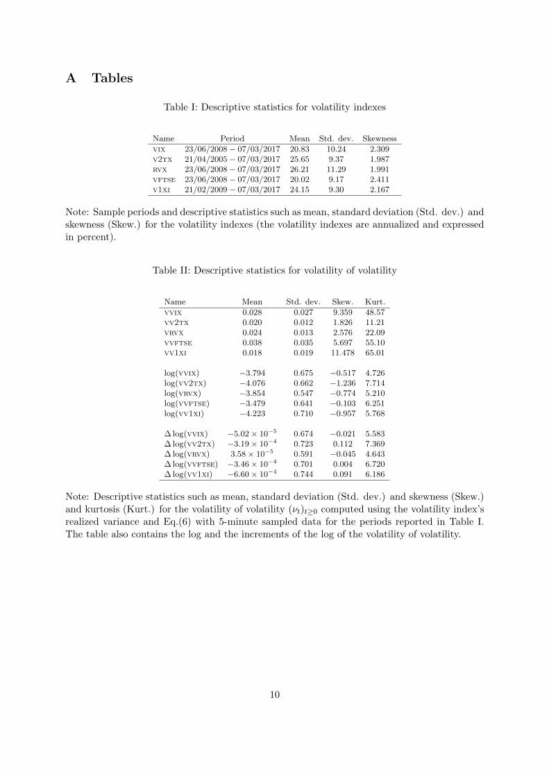
The data: We consider the volatility indexes: vix, v2tx, rvx, rvx and v1xi. The vix is the

volatility index computed from European S&P500 options, v2tx is the EuroStoxx50 volatility

index (also named VSTOXX), the rvx is the Russell 2000 volatility index that is computed

from options on that index, vftse if the FTSE volatility index and v1xi is the volatility index

computed from DAX30 options (also called the VDAX). Due to data constraints, these volatility

indexes are available for different time periods, we refer to Table I for the details. All the data

are sampled at a 5-minute frequency and simple descriptive statistics for these volatility in-

dexes are reported in that table. The mean values of the volatility indexes are all around 20% to

30% while standard deviations and skewnesses are approximately equal to 10 and 2, respectively.

[ Insert Table I here ]

For a given volatility index, its realized volatility of volatility is computed using Eq.(6) and basic

statistics such as mean, standard deviation, skewness and kurtosis are given in Table II. For

a given volatility index, its volatility of volatility is named by prefixing the volatility index’s

name by the letter “v”, so vvix stands for the volatility of volatility of the VIX while vv2tx

stands for the volatility of volatility of the V2TX. The other volatility of volatility indexes are

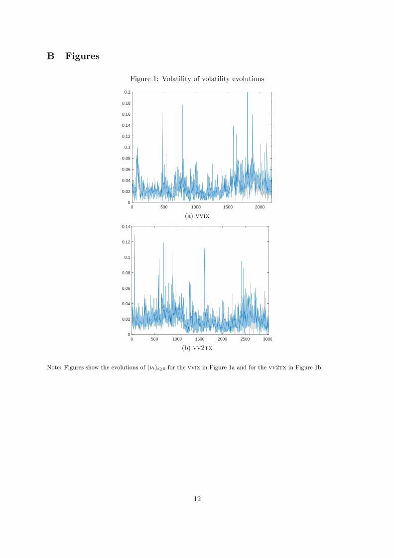
named accordingly. Figures 1 report the evolutions of vvix and vv2tx. Table II also reports

5

the statistics for each volatility of volatility index, the logarithm of the volatility of volatility

index as well as the increments of the logarithm of the volatility of volatility. The table shows

that mean values of the volatility of volatility indexes range from 0.018 for the vv1xi to 0.038

for the vvftse. This latter index also displays the highest standard deviation (i.e. 0.035).

Regarding the skewness and kurtosis, the vv2tx achieves the lowest values while the highest

values are achieved by the vv1xi. Taking the logarithm has the well known effect of reducing the

discrepancies between the variables and turns the distributions closer to the normal distribution.

Indeed, the skewnesses are much smaller and the kurtoses are closer to 3 (but still larger). Also,

of interest are the volatility of volatility log increments, the table II shows that the kurtoses

range from 4.6 to 7.3 while the skewnesses are very small and around 10−2 in absolute value

terms for all indexes but vv2tx that is equal to 0.112. The distributions of the logarithm of

the volatility of volatility increments for the vvix (upper figures) and vv2tx (lower figures) are

shown in Figure 2 for the two time intervals ∆ = 1 day and ∆ = 5 days. A Gaussian fit is also

reported for each distribution and shows that this approximation is reasonable (at least visually).

[ Insert Table II here ]

[ Insert Figures 1 here ]

[ Insert Figures 2 here ]

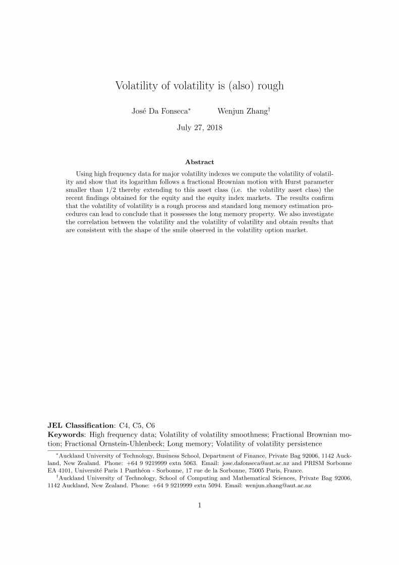
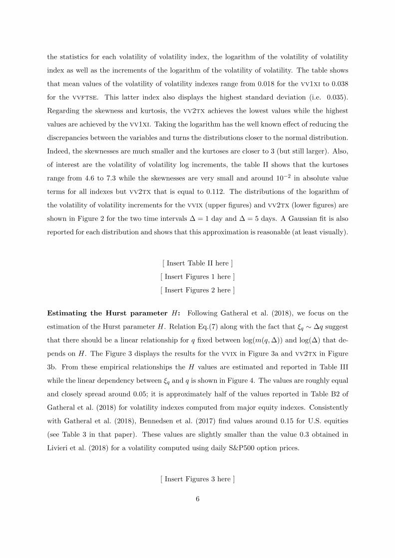
Estimating the Hurst parameter H: Following Gatheral et al. (2018), we focus on the

estimation of the Hurst parameter H. Relation Eq.(7) along with the fact that ξq ∼ ∆q suggest

that there should be a linear relationship for q fixed between log(m(q,∆)) and log(∆) that de-

pends on H. The Figure 3 displays the results for the vvix in Figure 3a and vv2tx in Figure

3b. From these empirical relationships the H values are estimated and reported in Table III

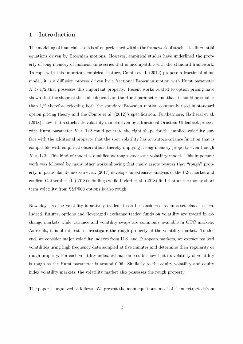
while the linear dependency between ξq and q is shown in Figure 4. The values are roughly equal

and closely spread around 0.05; it is approximately half of the values reported in Table B2 of

Gatheral et al. (2018) for volatility indexes computed from major equity indexes. Consistently

with Gatheral et al. (2018), Bennedsen et al. (2017) find values around 0.15 for U.S. equities

(see Table 3 in that paper). These values are slightly smaller than the value 0.3 obtained in

Livieri et al. (2018) for a volatility computed using daily S&P500 option prices.

[ Insert Figures 3 here ]

6

[ Insert Table III here]

[ Insert Figures 4 here ]

Autocovariance functions of the log of volatility of volatility: It was established in

Gatheral et al. (2018) that for t > 0 and ∆ > 0, if α → 0 in Eq.(3) then the following

approximation holds

cov(xαt , xαt+∆) = var(xαt )− 1

2ε2∆2H + o(1). (9)

In Figures 5, the autocovariance functions of the log of volatility of volatility log(νt) as a function

of ∆2H are reported. The Figure 5a is for the vvix with H = 0.06 while the Figure 5b is for the

vv2tx with H = 0.04. From the relation Eq.9, Gatheral et al. (2018) further show that when

αto0 then the following approximation holds

E[νt+∆νt] ∼ exp

(2E[xαt ] + 2var(xαt )− ε2

2∆2H

). (10)

As a result, the log(E[νt+∆νt]) is a linear function of ∆2H , this property is assessed empirically

in Figures 6, for the vvix it is Figure 6a with H = while for the vv2tx it is Figure 6b with

H = 0.04.

[ Insert Figures 5 here ]

[ Insert Figures 6 here ]

The correlation between the volatility index and its volatility: Thanks to the relation

Eq.(8) we evaluate the coefficient ρ, the results are reported in Table IV. All the correlations are

positive and range between 13% to 20%, it is consistent with the shape of the smile observed in

the volatility options market that is increasing. As the volatility market becomes more volatile

its volatility, thus the volatility of volatility, increases. It is a symmetric effect.

[ Insert Table IV here]

4 Conclusion

In this work we analyse the volatility of volatility indexes and show that its logarithm follows

a fractional Ornstein-Uhlenbeck process. For major volatility indexes, we compute the realized

volatility using 5-minute data and use it as a proxy for the instantaneous volatility of volatility

7

and estimate the Hurst parameter and find values around 0.05, roughly half of the values found

in the literature for equity indexes and equities. As for these two asset classes our results show

that the volatility follows a rough process. It has several consequences. First, it implies that

option pricing formulas for this framework have to be developed. Second, econometric estimation

procedures have to be built to take into account the fractional property of the process. Third,

combining Gatheral et al. (2018) and our results implies that there are two fractional levels, one

for the volatility and another one for the volatility of volatility, building a model that integrates

these two dimensions is an open and challenging problem.

8

ReferencesP.-O. Amblard, J.-F. Coeurjolly, F. Lavancier, and A. Philippe. Basic properties of the multivariate fractional

Brownian motion. ArXiv e-prints, 2012.

M. Bennedsen, A. Lunde, and M. S. Pakkanen. Decoupling the short- and long-term behavior of stochasticvolatility. arXiv:1610.00332v2, 2017.

F. Comte, L. Coutin, and E. Renault. Affine fractional stochastic volatility models. Annals of Finance, 8(2-3):337–378, 2012.

J. Detemple and C. Osakwe. The valuation of volatility options. European Finance Review, 4(1):21–50, 2000. doi:10.1023/A:1009814324980.

J. Gatheral, T. Jaisson, and M. Rosenbaum. Volatility is rough. Quantitative Finance, 18(6):933–949, 2018. doi:10.1080/14697688.2017.1393551.

S. L. Heston. A closed-form solution for options with stochastic volatility with applications to bond and currencyoptions. Review of Financial Studies, 6(2):327–343, 1993. doi: 10.1093/rfs/6.2.327.

G. Livieri, S. Mouti, A. Pallavicini, and M. Rosenbaum. Rough volatility: evidence from option prices. IISETransactions, 2018. doi: 10.1080/24725854.2018.1444297.

B. B. Mandelbrot and J. W. Van Ness. Fractional brownian motions, fractional noises and applications. SIAMReview, 10(4):422–437, 1968. doi: 10.1137/1010093.

Y.-H. Park. The effects of asymmetric volatility and jumps on the pricing of VIX derivatives. Journal ofEconometrics, 192(1):313–328, 2016. doi: 10.1016/j.jeconom.2016.01.001.

A. Sepp. VIX option pricing in a jump-diffusion model. Risk Magazine, 2:84–89, 2008.

9

A Tables

Table I: Descriptive statistics for volatility indexes

Name Period Mean Std. dev. Skewness

vix 23/06/2008 − 07/03/2017 20.83 10.24 2.309v2tx 21/04/2005 − 07/03/2017 25.65 9.37 1.987rvx 23/06/2008 − 07/03/2017 26.21 11.29 1.991vftse 23/06/2008 − 07/03/2017 20.02 9.17 2.411v1xi 21/02/2009 − 07/03/2017 24.15 9.30 2.167

Note: Sample periods and descriptive statistics such as mean, standard deviation (Std. dev.) andskewness (Skew.) for the volatility indexes (the volatility indexes are annualized and expressedin percent).

Table II: Descriptive statistics for volatility of volatility

Name Mean Std. dev. Skew. Kurt.

vvix 0.028 0.027 9.359 48.57vv2tx 0.020 0.012 1.826 11.21vrvx 0.024 0.013 2.576 22.09vvftse 0.038 0.035 5.697 55.10vv1xi 0.018 0.019 11.478 65.01

log(vvix) −3.794 0.675 −0.517 4.726log(vv2tx) −4.076 0.662 −1.236 7.714log(vrvx) −3.854 0.547 −0.774 5.210log(vvftse) −3.479 0.641 −0.103 6.251log(vv1xi) −4.223 0.710 −0.957 5.768

∆ log(vvix) −5.02 × 10−5 0.674 −0.021 5.583∆ log(vv2tx) −3.19 × 10−4 0.723 0.112 7.369∆ log(vrvx) 3.58 × 10−5 0.591 −0.045 4.643∆ log(vvftse) −3.46 × 10−4 0.701 0.004 6.720∆ log(vv1xi) −6.60 × 10−4 0.744 0.091 6.186

Note: Descriptive statistics such as mean, standard deviation (Std. dev.) and skewness (Skew.)and kurtosis (Kurt.) for the volatility of volatility (νt)t≥0 computed using the volatility index’srealized variance and Eq.(6) with 5-minute sampled data for the periods reported in Table I.The table also contains the log and the increments of the log of the volatility of volatility.

10

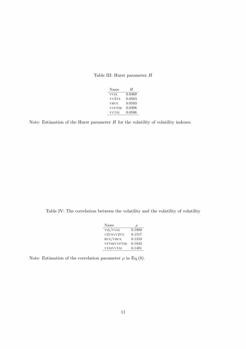
Table III: Hurst parameter H

Name H

vvix 0.0369vv2tx 0.0563vrvx 0.0593vvftse 0.0398vv1xi 0.0506

Note: Estimation of the Hurst parameter H for the volatility of volatility indexes.

Table IV: The correlation between the volatility and the volatility of volatility

Name ρ

vix/vvix 0.1989v2txvv2tx 0.1517rvx/vrvx 0.1310vftsevvftse 0.1843v1xivv1xi 0.1481

Note: Estimation of the correlation parameter ρ in Eq.(8).

11

B Figures

Figure 1: Volatility of volatility evolutions

0 500 1000 1500 20000

0.02

0.04

0.06

0.08

0.1

0.12

0.14

0.16

0.18

0.2

(a) vvix

0 500 1000 1500 2000 2500 30000

0.02

0.04

0.06

0.08

0.1

0.12

0.14

(b) vv2tx

Note: Figures show the evolutions of (νt)t≥0 for the vvix in Figure 1a and for the vv2tx in Figure 1b.

12

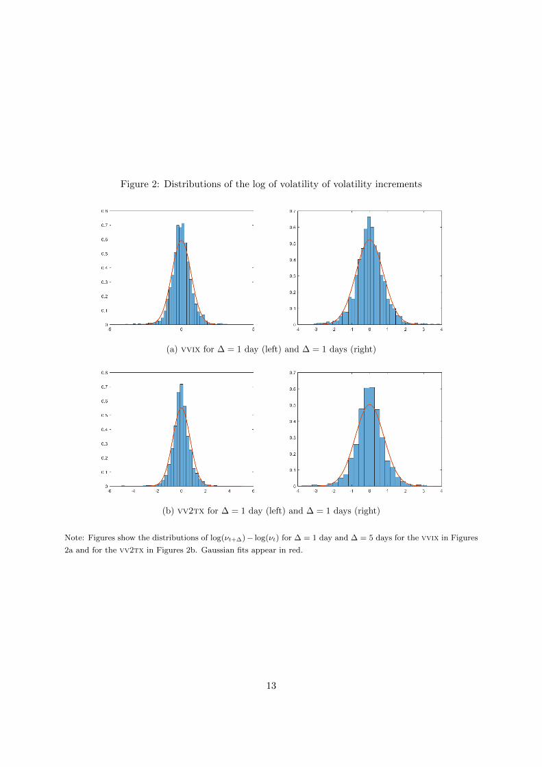
Figure 2: Distributions of the log of volatility of volatility increments

(a) vvix for ∆ = 1 day (left) and ∆ = 1 days (right)

(b) vv2tx for ∆ = 1 day (left) and ∆ = 1 days (right)

Note: Figures show the distributions of log(νt+∆)− log(νt) for ∆ = 1 day and ∆ = 5 days for the vvix in Figures

2a and for the vv2tx in Figures 2b. Gaussian fits appear in red.

13

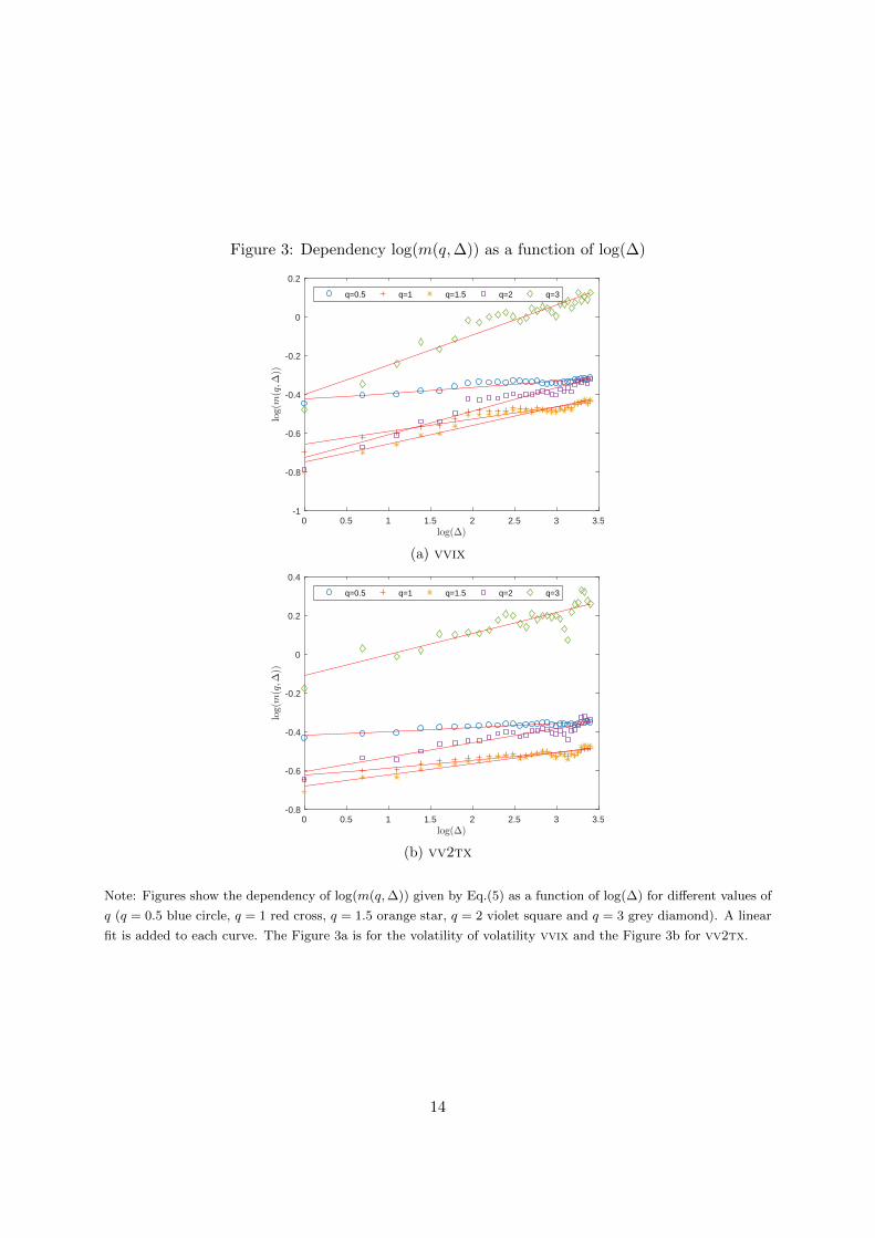
Figure 3: Dependency log(m(q,∆)) as a function of log(∆)

0 0.5 1 1.5 2 2.5 3 3.5-1

-0.8

-0.6

-0.4

-0.2

0

0.2

q=0.5 q=1 q=1.5 q=2 q=3

(a) vvix

0 0.5 1 1.5 2 2.5 3 3.5-0.8

-0.6

-0.4

-0.2

0

0.2

0.4

q=0.5 q=1 q=1.5 q=2 q=3

(b) vv2tx

Note: Figures show the dependency of log(m(q,∆)) given by Eq.(5) as a function of log(∆) for different values of

q (q = 0.5 blue circle, q = 1 red cross, q = 1.5 orange star, q = 2 violet square and q = 3 grey diamond). A linear

fit is added to each curve. The Figure 3a is for the volatility of volatility vvix and the Figure 3b for vv2tx.

14

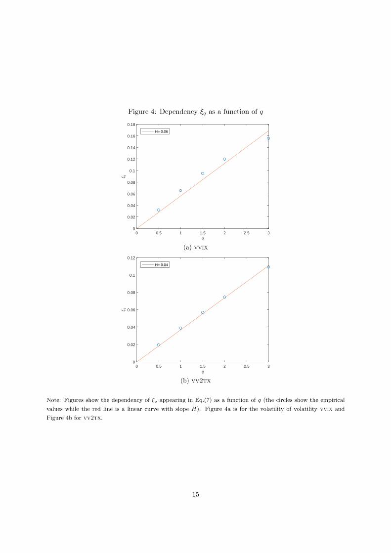
Figure 4: Dependency ξq as a function of q

0 0.5 1 1.5 2 2.5 30

0.02

0.04

0.06

0.08

0.1

0.12

0.14

0.16

0.18

H= 0.06

(a) vvix

0 0.5 1 1.5 2 2.5 30

0.02

0.04

0.06

0.08

0.1

0.12

H= 0.04

(b) vv2tx

Note: Figures show the dependency of ξq appearing in Eq.(7) as a function of q (the circles show the empirical

values while the red line is a linear curve with slope H). Figure 4a is for the volatility of volatility vvix and

Figure 4b for vv2tx.

15

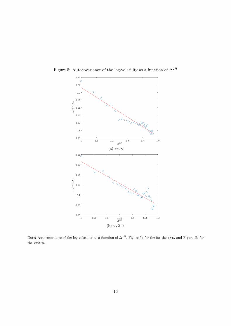
Figure 5: Autocovariance of the log-volatility as a function of ∆2H

1 1.1 1.2 1.3 1.4 1.50.08

0.1

0.12

0.14

0.16

0.18

0.2

0.22

0.24

(a) vvix

1 1.05 1.1 1.15 1.2 1.25 1.30.06

0.08

0.1

0.12

0.14

0.16

0.18

(b) vv2tx

Note: Autocovariance of the log-volatility as a function of ∆2H , Figure 5a for the for the vvix and Figure 5b for

the vv2tx.

16

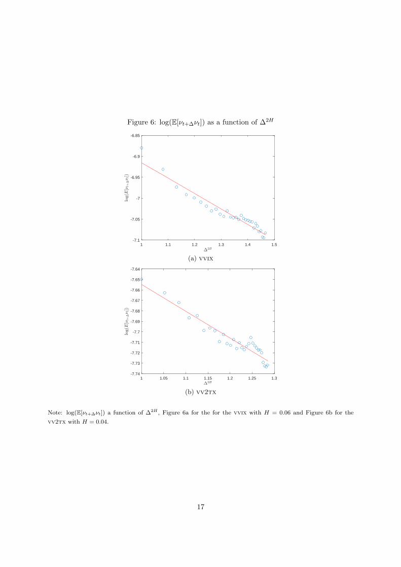
Figure 6: log(E[νt+∆νt]) as a function of ∆2H

1 1.1 1.2 1.3 1.4 1.5-7.1

-7.05

-7

-6.95

-6.9

-6.85

(a) vvix

1 1.05 1.1 1.15 1.2 1.25 1.3-7.74

-7.73

-7.72

-7.71

-7.7

-7.69

-7.68

-7.67

-7.66

-7.65

-7.64

(b) vv2tx

Note: log(E[νt+∆νt]) a function of ∆2H , Figure 6a for the for the vvix with H = 0.06 and Figure 6b for the

vv2tx with H = 0.04.

17