Embed Size (px)
Citation preview

NASA CONTRACTOR
REPORT
ROOT LOCUS DIAGRAMS BY DIGITAL COMPUTER
by Alh M. Krd und Robert Fonmro _. ,- :” ; i ,.’ . . ,I .. ‘C _ I.
Prepared by i ,... , ..’ . ’ : PENNSYLVANIA STATE UNIVERSITY
’ .:, ‘.’ ‘._ University Park, Pa. ‘/ _
* f Or \ _’
‘.._,’ NATIONAL AERONAUTICS AND SPACE ADMINISTRATION . WASHINGTON, D. C. “‘0. ‘%$liST 1966
https://ntrs.nasa.gov/search.jsp?R=19660024172 2018-09-02T04:45:21+00:00Z
TECH LIBRARY KAFB, NM
0099474 NASA CR-555
ROOT LOCUS DIAGRAMS BY DIGITAL COMPUTER
By Allan M. Krall and Robert Fornaro
Distribution of this report is provided in the interest of information exchange. Responsibility for the contents resides in the author or organization that prepared it.
Prepared under Grant No. NGR-39 -009-041 by PENNSYLVANIA STATE UNIVERSITY
University Park, Pa.
for
NATIONAL AERONAUTICS AND SPACE ADMINISTRATION
For sale by the Clearinghouse for Federal Scientific and Technical information Springfield, Virginia 22151 - Price $2.00

Introduction. Most continuously operating physical systems being
developed today are described by a system of differential equations. The
simplest of these are the linear systems, and the simplest of the linear
systems are those with constant coefficients. The concept of stability is
important in all such systems. In the last case, stability can be determined
by- examining the characteristic equation which is associated with each such
system.
There are several stability techniques available for systems with
constant coefficients: criteria due to Bode [l], Evans (Root-Locus) [3],
Michailov ['7], Neimark [g] and Pontrjagin [ll]. Each has its own advantages
and disadvantages.
The root locus method, which is to be discussed here, describes how to
construct the graph of the roots of the characteristic equation as one
parameter varies. This enables the designer to choose the positions of the
roots with some freedom, possibly achieving stability.
While most of the techniques are easily adapted for programming on a
digital computer, the root locus has proved more difficult. The purpose of
this article is to describe just how such a program was developed and to
show what information it gives.

The Root Locus. The root locus method has been developed for ordinary
systems and for systems with one time delay. We discuss the general system
(with delay). Let g(z) = zn + azn" + . . . . . . and h(z) = zm + bzm-' + . . . .
be polynomials with (constant) complex coefficients. Let Tando be
constant real numbers, T is 0, ose< 2Yf, and let K be real valued.
The characteristic equation we wish to consider is
F(z) = g(z) - -TZh(z) - Keiee = 0.
Definition. The root locus of F(z) is the set of all points z
such that z is a zero of h(z) or suchthat z is a zero of F(z) for
some real value of K.
The set of all points z on the root locus for values of K > 0 is
the positive root locus. The set of all points z on the root locus for
values of K < 0 is the negative root locus.
Theorem 1. The point z = x + iy is on the root locus of F(z) if
and only if @(x,y) = cos(e-my) Im (h(z)m ) + sin(e-7y) Re (h(z)m ) = 0.
Proof. Suppose z is on the root-locus. If g(z) # O>then for some
K # 0, h(z)Keiee-TZ/g(z) = 1. Thus
* h ') = K-1 e7X[cos(8 - my) - gz
i sin ((3 - Ty)].
h(z)g(z) = K-l eTx lk?(Z)12 [cos (e - Ty) - i sin (e - TY) 1 *
Since K, 7, x are real,
Re (h(z)m> = K-'eTx]g(z)12 cos (0 - my),

Im (h(z)m) = -K-1eTxlg(z)12 sin (e - Ty).
Multiplying the first by sin (e - Ty), the second by cos (e - Ty) and add-
ing completes the first part.
Conversely, if the equation is satisfied, then Im (el'e -7zh(z)g(z)) = 0.
So elee -TZh(z)m = R(z), where R(z) is real. If R(z) = 0, then
either h(z) = 0, or g(z) = 0, and z is on the root-locus. If
R(z) # 0, let K = ig(z)12/R(z). If K = 0, then g(z) = Oj and
Z is on the root-locus. If K # 0, then KeieemTZh(z)/g(z) = 1,and
F(z) = 0.
Note that K can be found by
K = eTxlg(z)12 cos (e - Ty)/Re(h(z)m),
or by
K = -e Txlg(z)12 sin (0 - I-y) /Id-ddg(z) > .
Lemma 1. Let h(z) and g(z) have real coefficients. Then
m h(z) = Cjzo h(j)(x) (iy)j / j! ,
m = cn j=O g(j)(x) (-iy)j/ jr .
Proof. These are just Maclaurin expansions.
Lemma 2. Let h(z) and g(z) h ave real coefficients. Then
n+m mj cj h(z)g(z) = C (-,pJk) (,jg(j-k) cx) .
j=O j: k=O
Proof. This follows from Lemma 1.
3

Lemma 3. If h(z) - and g(z) have real coefficients, then
Re(h(dg(z)) = xLco y&g PO ( 2; ) (-1)2k-$(i)(x)g(2k-i)(x),
(-l)k 2k+1 2k+l dh(dm) = m. & cico
Proof. This follows immediately from Lemma 2.
In any physical situation the coefficients of h(z) and g(z) must
be real, and 8 must be either 0 or aI. If K is permitted to take on
all real values, we lose no generality by fixing 8 at one of these values.
Since negative feedback is most frequently encountered, we let 8 = A .
Theorem 2. Let h(z) and g(z) have real coefficients, and let 8 = R.
Then z = x +iy is on the root locus of F(z) if and only if
fd(x, y) = cos Ty (-l)2k+l-ih(i)(x)g(2k+l-i)(x)
- sin * C" k=. 'w Z;ro e) (-l)2k-ih(i)(x)g(2k-i)(x) = 0.
The graph of this equation in the xy-plane is the root locus of F(z) l
The Root Locus by Digital Computer. AS might be anticipated, we will
use $(x,y) = 0 t o construct the root locus of F(z) rather than F(z)
itself. There are several reasons for this. First, in'the ordinary case
(7 = 01, we have no control over where the roots of F(z) might lie, so
factoring by machine is impractical. In the case with time delay (7 # 0),
F(z) = 0 has an infinite number of roots, and factoring is not possible.
In addition, the roots of F(z) = 0 do not vary at a uniform rate as
K varies. It is impossible to say in general how small the increments in
K should be in order to construct a reasonable graph.
On the other hand, $(x,y) = 0 does not involve K. On each vertical
line where x is fixed, the y coordinates of the root locus are the real
roots of @(X,Y> = 0. The procedure found to be most practical for determin-
ing those real roots y (where x is fixed) offers a direct means of
controling the error encountered in approximating these roots, and it works
just as well for systems with a time delay. It is as follows:
We choose any rectangular region in which the root locus is desired.
Let such a region be denoted by xR 5 x 5 xr, yb 5 y 5 yt. We divide
CX RJXrJ into increments xR,xR + Ax, xR + 2Ax, . . . . x . r For each point
XR + mAx in turn we divide [Yb'Yt] into increments in a similar manner,
yt>yt - &, yt - DAY, ..- yb- We then compute $(x,y) at these points,
first fixing x, then letting y vary from yt to yb- In so doing, for
a fixed x, we look for intervals in [Yb’Ytl over which ej(X,Y) changes
sign. The sign change indicates that a point of the root locus lies in the
interval. Each y interval where $(x,y) changes sign is divided in half,
and these subintervals are considered separately. The subinterval where #(x,y)
changes sign is itself divided in half, etc. In this manner the y
coordinate of the point on the root locus may be found quickly and accurately.
After the vertical strip from yt to yb has been exhausted and all the
points on the root locus have been found for that fixed value of x, x is
increased by Ax, and the process is repeated. As x varies from xR to
X r every point on the root locus in the rectangle is found. These points
are stored and then plotted by the computer.
The value of the parameter K is computed for each point on the root
locus using the formulas following theorem 1. The program plots + if
K>O, and-ifK<O. In addition, the triple (x,Y, K) is printed
out separately for each point on the root locus.
The program was designed for the IBM 7074 at the Computation Center
of The Pennsylvania State University, University Park, Pennsylvania, under
control of the Dual Autocoder Fortran Translator (DJJ'T) compiler system.
We hope that, with a minmum number of changes, it can be adapted for use
elsewhere.

FLOW CHART
START 7
v READ Y PARAMETERS
V INITIALIZE
READ COEFFICIENT / ROOT
VARIABLE = I EJ3TER
COMPUTE = G and H COEFFICIENTS (
FROM ROOTS I ENTER:1
READ G and H COEFFICIENTS
I
7

I COMPUTE INDEX LIMIT (= LIMIT)
-FOR COSINJ3 TERMS I
\L READ TAU
COMPUTE DERIVATIVES
OF G and H AT X
INITIALIZE
SPECIAL CASE NN52
FOR COSINE TERMS
COMPUTE COSINE
TERMS
8

j COMPl.WEFzEXXz;= LIMT)
COMPUTESINE
PRINT COEFFICIENTS e SEARCH
= INTERVAL [O, TOP]
FOR SIGN CHANGE I-
SEARCH INTERVAL
[YO, nl FOR SIGN CHANGE
3'
V
9

PRIMARY SEARCH FOR
SIGN CHANGES
\L COMPUTE K
d i ATTACH SIGN OF K
TO CORRESPONDING ROOT
RECORD NUMBER OF
ROOTS
v PRINT ROOTS
10
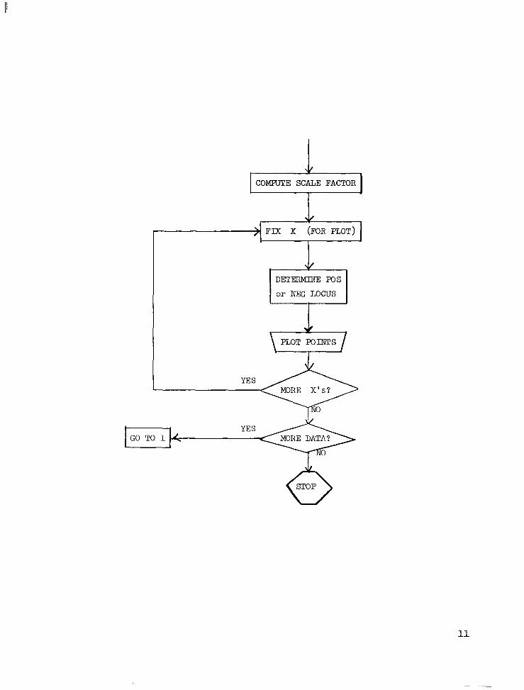
FIX X (FOR PLOT)
DEZZRMINEFOS
or NEG LOCUS
PLOT POINTS
MORE DATA?
11

Parameters Necessary for Execution : Data Cards
Card No. 1 Variable Names: DELTA, BGN, END.
Use: Determines points on real axis where coefficients of closed
form'ploynomial will be evaluated. Left hand endpoint BGN,
right hand endpoint END. The interval [BGN, EBD] divided
into subintervals of length DELTA. hraluation takes place
at each endpoint of these subintervals, i.e. at
EN, BGN-DELTA, EGN-2 DELTA, . . . , END.
Card format: columns l-10 numerical value of: DELTA PEAL K)DE,
n 11-20 I, EGN 1, ,
II 21-30 II END II .
Card No. 2 Variable Names: DEC, YO, Yl, TOP, ISIG.
Use: DEC: decrement to be used for isolation of roots.
yo,n: Allow detailed inspection of any interval along
Y-axis. YO < Yl. If their sum is zero (usual case),
program sets upper bound for roots (See comment).
TOP: Maximum value desired along vertical axis (Vertical scale
factor).
ISIG: Tolerance desired for roots is l@*(-ISIG), where
1 _< ISIG < 10.
Comment: The usual case is to set YO = 0.0; and Yl = 0.0, and
TOP = a (a some value). Occasionally detailed inspection
of some interval [a 1'"2] may be desirable al < a2 < a.
12

If the magnification factor is to be the same,set YO = al,
n = a2, TOP = al. To magnify, set YO = al, Yl = a2,
TOP = a2.
Card format: columns l-10 numerical value of: DEC REAL MODE,
I, 11-20 11 YO !1 ,
11 21-30 I, n ,I > II 31-40 I, TOP I,
,
column 45 II ISIG INTEGER MODE.
Card No. 3 Variable Name: IENTER
Use: A numerical value of 1 will cause the program to assume that
h and g are given in factored form and enter appropriate
routines to calculate their coefficients. Any other value will
cause the program to assume that the coefficients of h and
g are being provided directly.
Card format: column 5 1 Integer Mode,
columns l-5 any integer ff I, .
If card #3 contains the digit 1 in column 5 these data cards
must follow:
Card No. 4* Variable names (Used in COMPCO): M,N
Use: M- number of conjugate pairs of complex roots of g (must
be 5 6).
N- number of real roots of g (must be 5 12).
Card format: columns l-5 (right justified) M IJXJTEGES MODE,
II 6-10 " " N II .
13

Card No. 5*: complex roots of g
Card format: Columns real part
l-5
11-15
imaginarypart 6-10 REAL MODE,
16-20 II ,
21-25 26-30 II .
etc.
Card No. 6*: keal roots of g
Card format: Columns
l-5
6-10
etc.
REAL MODE,
II >
11 ,
II .
CardNo.7*and8*: ssmeas5* and 6* except information must pertain to
h.
If card #3 contains any integer in columns l-5 other than 1 in column 5
these data cards must follow:
Card No. 43Hc Variable Names: NG, NH
Use: NG- degree of g (must be 5 12).
NH- degree of h (must be 5 12).
Card format: columns l-5 (right justified) NG
6-10 " " NH
Card No. 5*: coefficients of g (highest power first)
Card format: columns l-10 coefficients of x n
11-20 fl n-l X
etc.
INTEGER MODE,
11 .
REAL MODE,
,l ,
14

Card No. 6~: coefficients of h
Card format: (same as 5*)
Card No. p (or 7*) Variable name: TAU
Use: Time Lag Parameter
Card format: columns l-10 RFAL MODE.
Card No. 1W (or 8**) Variable name: I STOP
Use: A numerical value of 1 will cause the program to
re-initialize itself, i.e., start over. A numerical value
of 2 will result in termination of execution. If the
program starts over, additional sets of data cards, as
described above, must be included in sequence.
Card format: column 5 INTEGER MODE.
15

THE PROGRAM
*tttY*t~~tttttttttttt~~tttttt*ttttt*ttttt~tttttttttttttttttttttttttttttttttttt +c IDENTIFICATION l c l C CHAR ,PLOT -- USED IN PLOTTING SECTION WC FRT -I FORMAT CONTROL +c 5 -- LEFT ENDPOINT OF SIGN CHANGE INTERVAL *c Y*C -- TEMPORARY STORAGE *-c A -- COEFFICIENTS OF POWERS OF Y l c X em POINTS ALONG X-AXIS l C YVAR e- POINTS TO BE PLOTTED +c NROO TS -- NUMBER OF ROOT LOCUS POINTS AT A GIVEN POINT ON X-AXIS l c CG -i COEFFICIENTS OF G AND ASSOCIATED DERIVATTVES *c CH -- COEFFICIENTS OF H AND ASSOCIATED DERIVATIVES l C NG -- ORDER OF G l C NH es ORDER OF H l c G PO VALUES OF G AN0 ASSOCIATED DERIVATIVES AT SORE POINT l C Ii -- VALUES OF H AND ASSOCIATED DERIVATIVES AT SOME POINT l c TAU -- TIME LAG +c KVAL me VALUES OF K FOR EACH POINT TO BE PLOTTED l c tc CHARACTER MODE = DAFT FEATURE... l C ADDRESSES EACH CHARACTER OF A STRING INDIVIOUALLY tt+t*tttttttt~ttttttttttttttttttt4ttttttttt&ttt*tttttttttttttttttttt*ttttttttt
CHARACTER CHAR~121,PLOTKl00~,Fnr(25~ DIMENSION S~12~rY~L2~,AI25~rX~2OO~,YVAR~l2,2OO~,NROOTS~2OO~,C~l5~ COMMON CGTl3r13~,CH~13,13~,NG,NH,G~26~,H~26~,TAU REAL KVAL(12)
*t4tttttt**tttt*tttttt**tttttttt*ttttt*tttt*t*ttttttttttttt*tttttttttt**tttttt
+c
l c INITIALIZATION 4C *t4.+ttttttttt*ttttt*t*ttttttttttt*ttttt**tt*t**ttttt*tttttttt*t*t+*ttt*ttttttt
10 DO 12 I-l,200 NROOTSt I a=0 X~I?=O.O 00 12 J=l,12 YVARiJ,I)=O.O
12 CONTINUE DO 13 I=l,lOO
13 PLOTL I l=lH PRINT 14
14 FORHAT~lHlrlOX~ t*4tttt*tt*ttttt*ttttt*tttttt*tttttttttttt**tttt*tt4tttttt*ttttttttt*ttttttttt
+C READ X PARAMETERS *C DELTA -P X-AXIS INCREMENT 4c BGN -- LEFT POINT X-AXIS tc END PB RIGHT POINT X-AXIS *t4t*m*+ttt,4ttttt+tttttttt*ttttt*tt**tttttttttttttt*t*t*tttttttttttt*tttttttt
READ 100. DELTA. BGN.END 100 FORMATl3FlO.O)
17
-
tttttttttttttttttttttttttttttttttttttttttttt*tttttttt4tttttttt*ttt4ttttttttttt
*c l c COMPUTE X-AXIS POINTS l c ttt*tttttttttttttttttttttttttttttffttttttt4ttttttt*ttttttttttttttttttttttttt*tt
M=ABS(BGN-ENDI/DELTA+l.O XI l)=BGN IFtM-200) 7s 7, 8
8 H=200 7 DO 9 I=2,H 9 Xt I )=X( I-ll+DECTA
ttttt~tttttttttttttttttttttttttttttttttttttttttttttttttttttttt*ttttttttttttttt l c READ Y PARAMETERS l c DEC -- ROOT SEARCH INCREMENT l c YOIYl -- PERMIT DETAILED INSPECTION OF Y-AXIS l C TOP -- UPPER BOUND FOR ROOTS (SCALE FACTOR ON VERTICAL) *c ISIG -- ROOT TOLERANCE..E=lO**I-ISIGT **ttt~t*tttttttttttttttttttttttttttttttttttttttttttttttttttttttttttttttttttttt
READ l1O,DEC,YO,YlrTOP.ISIG 110 FORHAT(4FlO.O,15)
ttttttttttttttttttttttttttttttttttttttt+tttttttttttttttttttttt+ttttttttttt~ttt l c COMPUTE TOLERANCE FOR ROOT ERROR AND l c OBTAIN CORRESPONDING FORMAT STATEMENT ttt,t~ttttttttt+~ttttttttttttttttttttttttttttttttttttttttttttttttttttttttttt~t
E=(lO.O)**(-ISIG) CALL FRMATTFMT,ISIG~
tttttttttttt*ttttttttttttttttttttttttttttttttttttttttttttttttttttttttttttttttt l c l c INITIALIZATION l c ttt+t~ttttttttttttttttttttt*tt+ttttttttttttttttttttttttttttttttttttttttttttttt
DO 15 1=1,13 DO 15 J=1,13 CH(I,Jl=O.O
15 CGtI,J)=O.O ***+t~tttttttttt~tttttt+ttttt*tttttt~ttttttttttttttttttttttttttttttttttttttttt l c l c COEFFICIENT/ROOT OPTION l c tttttttttttttttttttttttttttttttttttttttttttttttttttttttttttttttttttttttttttt~t
READ 97,IENTER IFiIENTER-1) 17, 16, 17
ttt*t4tttt+tttttttttttt*tttttttttttttttttttttttttttttttttttttttttttttttttttttt +c l c COMPUTE G COEFFICIENTS FROM ROOTS (IENTER= l c *ttQt*ttttttttttttt*tt+tttttttttt4tttt*t*ttt*tttt*tttttttttttttttttttttttttttt
16 PRINT 99 99 FORMATt 1H rl2HFACTORS OF G)
CALL COMPCOfC,NGl) NG=NGl-1 DO 18 I=lrNGl
18 CGll~I~=C(I~

tttttttttttttttttttttttttttttttttttttttttttttttttttttttttttt+ttttttttttttttttt~ +c l c COMPUTE H COEFFICIENTS FROM ROOTS (IENTER= l c ttttt*tttttttttttttttttttttttttttttttttttttttttttttttttttttttttt*tttt*tt*ttt*ti
PRINT 98 98 FORHATtlH rl2HFACTORS OF HI
CALL COMPCO(C,NHl) NH=NHl-1 DO 19 I=l,NHl
19 CHIl,I~=C~I~ GO TO 20
tttttttttttttttttt*tttttttttttttt*tttttt&tttttttttttttttttttttt*ttt*tttttttttt4 l c l c READ COEFFICIENTS OF G AND H LIENTER=O) +c ttttttt*ttttttttttttttttttttttttttttttttttttttttttttttttttttttttttttttt*tttt*t~
17 READ 97,NG,NH 97 FORMATIZIS)
NGl=NG+l NHl=NH+l READ 96,(CG(l,I~,I=l,NG1~ READ 96,(CH(l,Il,I=l,NHlI
96 FORMAT(BFlO.0) tttttttttttttttttttttttttttttttttttttttttttttttttttttttttttttttttttttttttttttt4 l c +c COMPUTE DERIVATIVE COEFFICIENTS AND PRINT l c tttttttttttttttttttttttttttttttttttttttttttttttttttttttttttttttttttttttttttttt4
20 NlG-NGl 00 21 1=2,NGi NlG=NlG-1 DO 21 J=l,NlG CGfI,J)=FLOAT(NlG+l-J)tCGo
21 CONTINUE NlH=NHl DO 22 1=2,NHl NlH=NlH-1 DO 22 J=l,NlH CHII,J~=FLOAT~N1H+1-J)+CHo
22 CONTINUE PRINT 95 r(lCG(I~J~rJ=lrl3~rI=l,l3~ PRINT 94 ,I(CHIIrJ~rJ=lsl3~rI=lt13)
95 FORMATISOH COEFFICIENTS OF G AND ASSOCIATED DERIVATIVES // l(lH ,12FlO.l,F9.lII
94 FORMATLSOH COEFFICIENTS OF H AND ASSOCIATED DERIVATIVES B/ l(lH r12FlO.l,F9.1)1 ttttttttttttttttttttttttttt~*tttttttttttttttttttttttttttttttttttttttttttttttttt
+c +c SUMMING INDEX . ..NN=DEGREE OF Y POLYNOMIAL *c tttttttCttttttttt,ttttttttttttttttttttttttttttttttttttttttttttttttttttttttttttt
NN=NG+NH LIMIT-INN-lI/2
19

IF(LIMIT-$1)26,26,27 27 PRINT 93,NN 93 FORMAT1 @ DEGREE OF POLYNOMIAL (‘,12,‘1 EXCEEDS PROGRAM LIMIT')
STOP 26 READ 92,TAU 92 FORHAT(FlO.0)
DO 28 IM=l,M CALL COHPDERIV(X(IM)I
tttYttttttttttttttttttttttttttttttttttttttttt*tttttttttttttttttttttt*ttttttt~4
l c l C INITIALIZATION +c ttttttttttttttttttttttttttttttttttttttttttttttttttttttttttttttttttttttttttfftt4
DO 11 I=1112 S(Il=O.O Y(II=O.O
11 CONTINUE DO 29 I=lr25
29 A(I)=O.O ttt~t4ttttttttttttttttttttttttt4tttttttttttttttttttttttttttttttttttt~tttttttt4
l c l c Y COEFFICIENT CDMPUTATION..COSINE TERMS +c ttttfftttttttttttttttttttttttttttttttttttttttttttttttttttttttttttttttttttttttt4
IFtNN-2)31,31,32 31 KK= 1
KI=NN DO 33 I=O,KK KIK=KK-I A~K1l=AIKI~+COMB~KK,I~*~-l.O~**KIK*H~I+l~/FACT~KK~*G~~KIK+l~
33 CONTINUE GO TO 34
32 DO 35 K=O,LIHIT KK=2*K+l Cl=(-l.Dl**K KI=NN+l-KK DO 36 I=O,KK KIK=KK-I A~KI~=A~KI~+COMB~KK,I)+o l *KIK*HII+1~/FACT~KK~*G~KIK+l~
36 CONTINUE A(KI)=AIKI)*Cl
35 CONTINUE ttttt4ttttttttttttttttttt*ttttttttttttttttttttttttttttttttttttttttttttttttttt4 +c d-4 COMPUTATION OF SINE TERMS l c +tt,ttttttttttttttttttttttttttttttttttttttttttttttttttttttttttttttttttttttttt4
34 IF(TAU)37,38,37 37 LIMT =NN/2
A(NN+lT=H(l)*G(ll IFLLIMT 138.38.39
20

39 DO 40 K=lrLIMT Cl=(-l.O)**K KK=Z*K KI=NN+l-KK DO 41 I=O,KK KIK=KK-I A~KI~=A~KI~+COM6~KK,I~*~-l.O~**KIK*H~I+1~/FACT~KK~*GfKIK+l~
41 CONTINUE A(K1 )=A(KI )*Cl
40 CONTINUE ttt*tttttttttttttttttttttttttttttttttttttttttttttttttttttttttttttttttttttttttt l c +c PRINT Y COEFFICIENTS l c tttttttttttttttttttttttttttttttttttttttttttttttttttttttttttttttttt4*ttt4t*t4t*
38 Nl=NN+l PRINT 112rXfIH~,(A~I~,I=l,Nl~
112 FORHATtlH ///ZZHOCOEFFICIENTS FOR X= ,F6.2//(15X,E15.8)) N=NN IF(YO+Y1)42r55,42
55 Yl=TOP YO=O.O
ttttttttttttttttttttttttttttt*tttttttt4tt*ttttttttttt*ttttttttttttttttttttt*tt
+c
64 PRIMARY SEARCH FOR SIGN CHANGES l c ttttttttttttttttttttttttttt*ttttttt4tttttttt4tttttttttttttttttttt**tttttt**4t*
42 CALL SEARCH~YO,Yl,DEC,S,J,A,N~ IF(J) 43,43,44
43 PRINT 102 102 FORMAT(‘OSEARCH NEGATIVE’)
GO TO 28 ttttttttttttttttttttttttttttttttttttttttttttttttttt*ttttttttt*ttttttttttttttt4 +c l C FINAL ROOT COMPUTATION +c K COMPUTATION l c *t****tttt*t**t*t**t*t**t**t**t*ttt***t*t*t4*tttt*ttttttttt*tt**t**tttt**t*t4*
44 K=O GO 45 I=lrJ XL=SlI) CALL ROOT tXL,DEC, A,N,E,AROIJT) K=K+l YTKb=AROOT KVAL(K1=COMPK(AROOT,Xo) YVAR~KoIM~=SIGN(AROOT~KVAL~K)I
ttttt*ttttttttttttttt*ttttttttttttttttttttttttttttttttttttttttttt*ttt*t4t*t*tt
l c l c 5IGNtA.B) .,-RETURNS VALUE OF A HITH SIGN OF B l c *t4ttttttttttt*tttttt*ttttttttttttttttttttttttttt*tttttttttttttttt4t**4*t*tttt
45 CONTINUE
21

NROOTSf IMl=K PRINT 113
113 FORMAT{ ‘OROOTS ARE’) PRINT FHT,~Y(I~,KVAL~I~,I=l,K~
28 CONTINUE ttt*t+4ttt*ttttttttttttttttttt*tttttttttttttttttttttttttttttttttttttttttttttttt
4C SCALiNG AND GRAPHING +c +c SCALE AND GRAPH... 4C SYSTEMS LIBRARY ROUTINES WHICH WILL SCALE DATA AND +c SET UP PLOT ARRAY AS 100 CHARACTER IMAGE l C OF LINE TO BE PRINTED **~+t~t*t*tt4~tt~t*tttt4*tt*t*t~4*tttt*4ttttt*tt~tttttttttttttt~ttttttttttttttt
80 81 47
51
50 49 48
90 46
88
89
52
PRINT 14 FACTGR=(TOP-YOE/lO.O CALL SCALE~YO,FACTOH,YO,FACTOR,YO,FACTOR,YO,FACTOR,YO,FACTOR
1 ,Y0,FACT0RsY0,FAtT0R,Y0,FACT0R,Y0,FACT0R,Y0,FACT0R 2 ,YO,FACTORIYOIFACTOR)
DO 46 KK=lrM 00 47 I=lr 12 IF~YVARII,KK~~8lr80,8l YVAR(I,KK)=YO CHARII)=lH CONTINUE K=NROOTS(KK) DO 48 I=lrK IFIYVAR(I,KK~)50,51,51 CHAR(I)=lH+ GO TO 49 CHARl I )=lH- YVARIT,KK)=ABSTYVARiI,KKi1 CONT! NUE CALL GRAPH%PLG~,YVAR~lrKK~rCHAK~l~rYVAR~2~KK~rC~AR12~,YVAR~3,KK~,
lCHAR(31,YVPRi4,KK~rCHARI45rYVAR1SrKK)rCHAR~5~~YVAR~6~KK~,CHAR(6~, ZYVARi7,KK1,CHAR~7),YVARI8rKK)rCHAR[8)rYVAR~9,KK),CHAR(9),YVAR(lO, 3KK~,CHAR~10~,YVAR~11,KK~,CHAR~11~,YVAR~12,KK~,CHAR~12~~
PRINT 90sXfKKlrPLOT FGRMAT~lHS~F10.2,5XslOOC~ CONTINUE PRINT 88 FORMAT(16X,“be,98X,‘S’1 PRINT 89,TOPvFACTOR FORMAT(l6X,3H0.0,94X,F4.1/17HGSCALE FACTOR IS rF’+.ltlbH UNITS PER
1 INCH) READ 97rISTOP GO TO Ll0,52)rISTUP STOP
22
SUBROUTINE COMPCOtC,NN) ttt*tttttttttttttttttttttttttttttttttttttttttttttttttttttttttttttttttttttttt*t l c SUBROUTINE READS IN REAL AND/OR COMPLEX ROOTS AND COMPUTES +c COEFFICIENTS OF THE RESULTING, POLYNOMIAL. l c l c C = ARRAY OF COEFFICIENTS +c NN = DEGREE OF POLYNOMIAL+1 *ttttttttttttttttttttttttttttttttttttttttttttttttttttttttttttttttttttttttttt*4
9
1
2
3
100
25
200
26 28 27
201 32 101 31
10
11
12
17 35
CHARACTER FHDI51 DIMENSION CRTSf6,2~rRRTS~121rC(15),Ao DATA FMD/‘(Z -(@I DO 9,X=1,15 0(X)=0.0 C(I)=O.O DO 1 Jrl.6 DO 1 I+112 CRTS(J,I)=O.O DO 2 J=l,12 RRTS(Jl=O.O DO 3 J=1,6 DO 3 1=1,13 A(J,I)=O.O LOW1 IN=1 II=2 READ 1OO.M.N FORMATI IFIMI25.26.25 READ 10lrl(CRTS(I,J~,J=l,2)rI=lrM) PRINT 200,(FHD,(CRTS~I,J~rJ=l,2~,I=l,M~ F0RMAT~1H0,6~5C,F5~1,3H+/-,F5.1,3H1~~~~ GO TO 28 II=1 IF(N127r32.27 READ lOl,(RRTS~I~rI=lrN~ PRINT 201 r(FMD,RRTS~I~,I=l,N~ FORMAT(lHO,10(5C rF5.1,2H)))1 GO TOf30,31),11 FORMATf16F5elI DO lO,I=lrM A(I,l)=l.O AfIr =-2.O*CRTS(I.l) A(I,3~=CRTS~I,1~**2+CRTSo++2 DO 11,1=1,3 CII)=Afl,I) 1F~M-1~12,16r12 J=2 LIM=3 DO 35,I=l,LIM D(I)=C(II LIM=LIM+Z
23
DO 15, I=lrLIM C(I)=O.O DO 15,K=l, I
15 ClI~=C(I~+AIJ,K~*D(I+l-Kl J=J+l IFtH-JIl6,17,17
30 C~l)=l.O C(Z)=-RRTSfll LOWL IH=2 NN=2 GO TO 18
16 NN=2*M+l IF(N118r19.18
18 IF(LOWLIM-NI50,50,19 50 00 20 J=LOWLIH,N
T=-RRTSfJI NN=NN+l DO 20,K=l,NN Tl=- RRTS(J)*C(K+l) C(K+l)=T+C(K+ll T=Tl
20 CONTINUE 19 RETURN
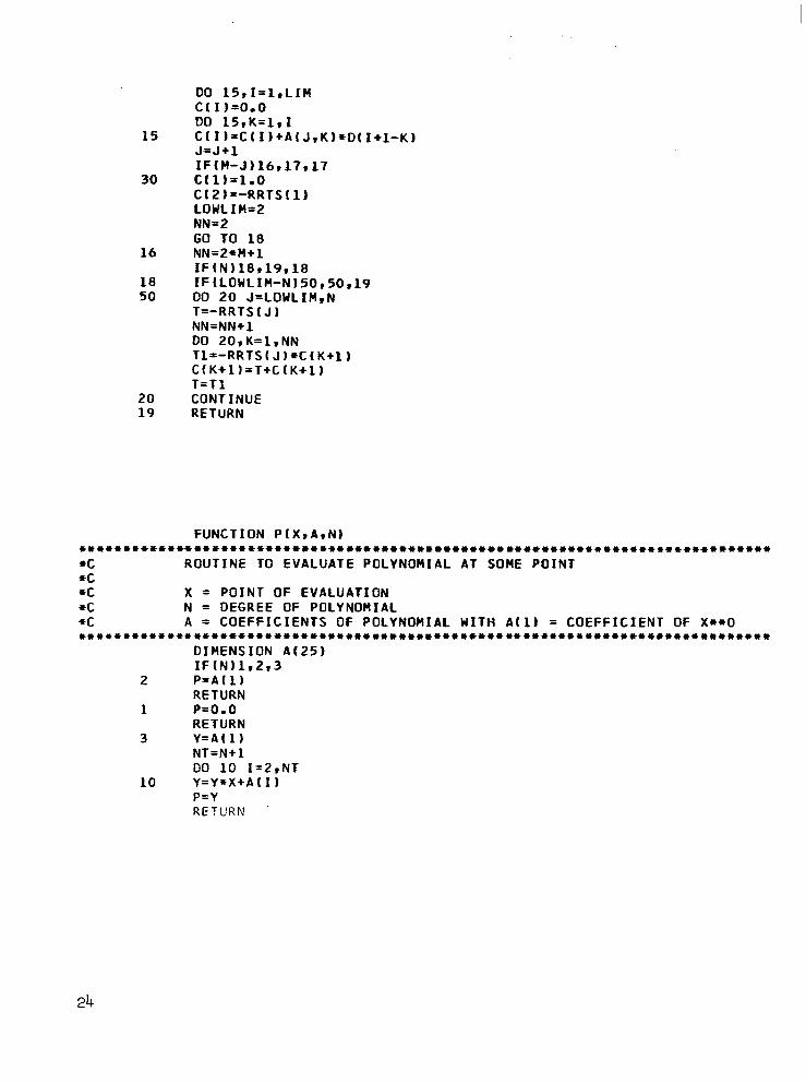
FUNCTION P1X.A.N) t4ttttttttttttttttttttttttttttttttttttttttttttttttttttttttttttttttttt*4ttttttt
l c ROUTINE TO EVALUATE POLYNOMIAL AT SOME POINT l c l c x = POINT OF EVALUATION l c N = DEGREE OF POLYNOMIAL 4c A = COEFFICIENTS OF POLYNOMIAL WITH A(1) = COEFFICIENT OF X*+0 ttttttttt4tttttttttt4tttttttttttt4tttttttttttttttttttttttttttttttttttttttttttt
DIMENSION Al251 IF(N)lr2,3
2 P=A(l) RETURN
1 P=O.O RETURN
3 Y=A(l) NT=N+ 1 DO 10 1=2,NT
10 Y=Y*X+A(I) P=Y RETURN
24
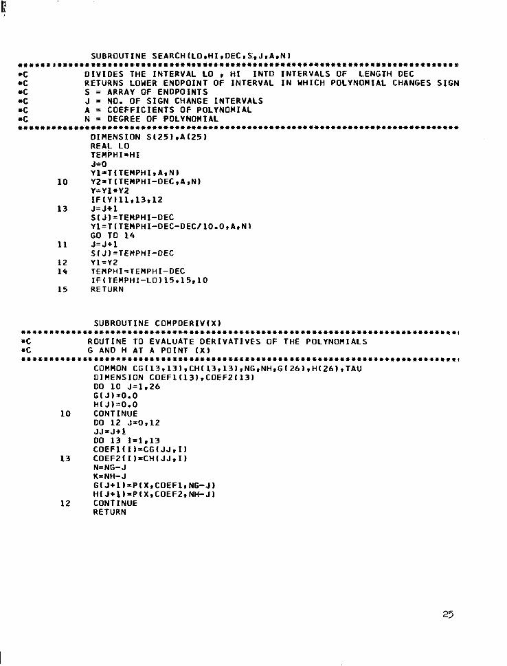
SUBROUTINE SEARCH~LO,HI,DEC,S,J,A,N~ tttttt,ttttttttttttttttttttttttttttttttttttttttttttttttttttttttttttt4*ttt4ttttt
*c DIVIDES THE INTERVAL LO , HI INTO INTERVALS OF LENGTH DEC l c RETURNS LOWER ENDPOINT OF INTERVAL IN WHICH POLYNOMIAL CHANGES SIGN l c S = ARRAY OF ENDPOINTS +c J = NO. OF SIGN CHANGE INTERVALS tc A = COEFFICIENTS OF POLYNOMIAL l c N= DEGREE OF POLYNOMIAL ttt*ttttttttttttttttttttttttttttttttttttttttt4fftttttff4ttttttttttttttttttttttttt
DIMENSION S(25IrAt25) REAL LO TEMPHI=HI J=O Yl;T(TEMPHI,A,N)
10 Y2=T(TEMPHI-DEC,A,N) Y=Yl*YL 1FIY~11,13,12
13 J=Jtl S(J)=TEMPHI-DEC Yl=T(TEMPHI-DEC-DEC/lO.O,A,Nl GO TO 14
11 J=J+l S(Jl=TEMPHI-DEC
12 Yl=Y2 14 TEMPHI=TEMPHI-DEC
IFtTEMPHI-LO)l5,15,10 15 RETURN
SUBROUTINE COHPDERIVtX) tttttttttttttttt4tt4tttttttttttttt*ttttt4tttttttt*ttttttt*tttt4ttttttttttt4ttti
*C ROUTINE TO EVALUATE DERIVATIVES OF THE POLYNOMIALS 4c G AND H AT A POINT (Xl tttttt*t*4ttttttt4ttttttttt4ttttttt4ttttt*tttttt*t4ttttttttttttt*tttttttttt*t*4
COMMON CG(13.13~,CH(13,13~,NG,NH,G~26)rHorTAU DIMENSION COEFl113),COEF2l131 DO 10 J=1.26 GK JbrO.0 H( J)=O.O
10 CONTINUE DO 12 J=O,12 JJ=J+L DO 13 I=lr13 COEFL(Il=CG(JJ,I)
13 COEFE(I)=CH(JJ,I) N=NG-J K=NH- J G(J+l)=P(X,COEFl,NG-J) H( J+ll=PlX,COEFZ,NH-JI
12 CONTINUE RETURN
25
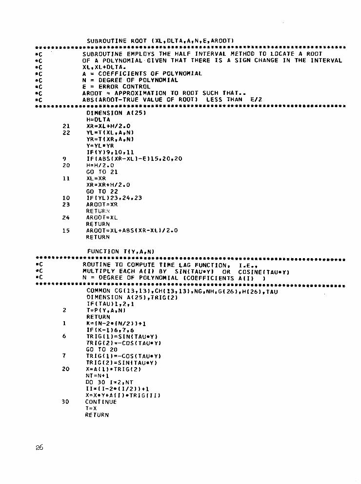
SUBROUTINE ROOT (XL,DLTA,A,N,E,AROOT) *t***,t*t4tttt*t****ttt44tttttt4tttttt4t4tttttttt*ttt**4tt**tt4tt*ttt*tttttt~4
l c SUBROUTINE EMPLOYS THE HALF INTERVAL METHOD TO LOCATE A ROOT l c OF A POLYNOMIAL GIVEN THAT THERE IS A SIGN CHANGE IN THE INTERVAL l c XL, XL+DLTA. l c A = COEFFICIENTS Of POLYNOMIAL l c N = DEGREE, OF POLYNOMIAL l c E = ERROR CONTROL l c AROOT = APPROXIMATION TO ROOT SUCH THAT.. l c A85 ( AROOT-TRUE VALUE OF ROOT) LESS THAN E/2 ~~t~~~tt~ttttttttttttttttttttttttttttttttttttttttttttttttttt44ttttt~tttttttt~t
DIMENSION A(251 H=DLTA
21 XR=XL+H/2.0 22 YL=T(XL,A,N)
YR=T(XR,A,N) Y=YL*YR IF(Y)9,10,11
9 1F(A85(XR-XL~-E~15,20,20 20 H=H/2.0
GO TO 21 11 XL=XR
XR=XR+H/Z.O GO TO 22
10 IF(YL)23,24,23 23 AROOT=XR
RETURh! 24 ARGOT=XL
RETURN 15 ARDOT=XL+ABS(XR-XL)/2.0
RETURN
FUNCTION TIY,A,N) tttttItttttttttt*ttt*ttttttttttttttttt4tt4ttttttttttttt**ttt4*4**4t**t***t*4tt
l c ROUTINE TO COMPUTE TIME LAG FUNCTION, IiE., l c MULTIPLY EACH A(I) BY SiN(TAU*Yl OR COSINEf TAU*Y) l c N = DEGREE OF POLYNOMIAL (COEFFICIENTS A(I) ) tttt4t4t4ttttttttttttttttttt4ttttttttt*t**t**t*t******4*4t*t****t*tt***t*t4t*t
COMMON ~G(13r13~,~H~13,13~,NG,NH,G~26)rH!26]1TAU DIMENSION A(251rTRIGL2)
7
20
30
IF(TAU)l,2,1 T=P(Y,A,N) RETURN K=fN-2*1N/2))+1 IF(K-1)6,7,6 TRIG(l)=SIN(TAU*Y) TRIG(Z) =-COSITAU*Y) GO TO 20 TRIG(l) =-CO5 (TAU*Y) TRIG(Z)=SIN(TAU*Y) X=AI$)*TRIGtZ) NT=N+ 1 DO 30 1=2rNT II=(I-2+(1/2)1+1 X=X+Y+AfI)+TRIGIII) CONTINUE T=X RETURN
26
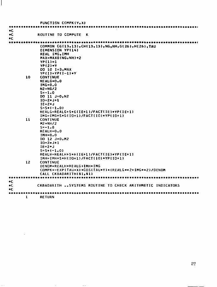
FUNCTION C0MPKfY.X) ttttttttttttttttttttttttttttttttttttttt4*ttt4ttttttttttt**ttt***tt*tttt*tt*ttt~
l c l c ROUTINE TO COMPUTE K l c ttttttttttttttttttttttttttttt4tttttttttttttttttttttttttttttttttt4ttttttttttttt4
COMMON CG~13,13~,CH~13,131,NG,NH,Gf26I,H~26)rtAU DIMENSION YP(14) REAL IMG,IHH HAX=MAXOtNG,NH)+2 YP(l)=l YP(2)-Y DO 10 1=3,MAX YP(I)=YP(I-lI*Y
10 CONTINUE REALGsO.0 IMG=O.O N2=NG/2 s=-1.0 DO 11 J=O,Nt 10=2*J+l IE=ZI*J S=S*f-1.0) REALG=REALG+S+GIIE+1)/FACT(IE)+YP(IE+l~ IMG=IMG+S*G~IO+1~/FACT(IO)rYP(IO+l~
11 CONTINUE M2=NH/2 s=-1.0 REALH=O.O IMH=O.O DO 12 J=O,M2 10=2*J+l IE=Z+J S=S*(-1.01 REALH=REALH+S*H~IE+1)/FACT(IE~*YP~IE+l~ IMH=IMH+S*HIIO+1~/FACTorYP(IO+l~
12 CONTINUE DENOM=REALH*REALG+IMH*IMG COMPK =-EXP(TAU*X~*COS~TAU*Y~*~REALG**2+IMG**2~/DENOM CALL CKBADARITHTSl,Sl~
ttt~**tttttt*tt*t*tttt~t4tttt*tttttt4~4t4tttttttttttt*ttt4tttttt44ttt44*tttt~t4
4c
l c CKBADARITH ..SYSTEMS ROUTINE TO CHECK ARITHMETIC INDICATORS l c tttttt4ttttttttttttttttttttttttttttttttttttt4t4tt4tttttttttttttttt4ttttttttt4t4
1 RETURN
27

SUBROUTINE FRMATtFMTiISIGJ tttYttttttttttttttttttttttttttttt4ttttttttttttt4tttt4ttttttttt*ttttttttttttttt
l c l c FORMAT CONTROL SUBROUTINE l c tttttttttttttttttttttt*tttttttttttttttttt*tttttt4tttt*tttttttttt*ttttttttttttt
CHARACTER FMT(25l,FHD(9),FMAT(25) DATA FMAT/,(9X,F14.6,9X,3HK =,El7.81'/,FMD/'123456789'/ DO 10 1=1,25 FMT(I)=FMAT(II
10 CONTINUE FMT( 9)=FHD(ISIG) RETURN
28

Examples
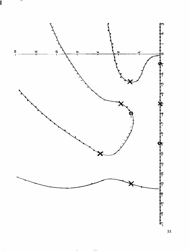
The following diagrams are the root-loci for g(z) + KemTZh(z) = 0
where
g(z) = (z + 5)(z + 3 + 3i>(z + 3 - 3i)(z + 5 + 4i)(z + 5 - 4i)
l (z + 10 + 6i)(z + 10 - 6i)(z + 13 + 3i)(z + 13 - 3i),
h(z) = (Z + l)(z + a)(z + 6 + 3i)(z + 6 - 3i), T is successively
0, l/4, l/2, 1,ana 2.
29

t
30
31

32


‘r +
\ +
\ +
+
\
+
\ \I \
+ +
t
34
REFERENCES
1. H. W. Bode, "Network Analysis and Feedback Amplifier Design," D. Van
Nostrand Co., New York, 1948.
2. W. R. Evans, "Graphical Analysis of Control Systems," Trans. A.I.E.E.,
67, (1948) ppe 547-551.
3. , 'Control System Synthesis by the Root-Locus Method,"
Trans. A.I.E.E., 69, (1~01, PP. 66-69.
4. A. M. Krall, 'An Extension and Proof of the Root-Locus Method,"
Jour. S.I.A.M., 9, (1%) PP. 644-63.
5. , "A Closed Expression for the Root Locus Method," Jour.
S.I..A.M., 11, (l%l), pp. 700-704 l
6. , "Stability Criteria for Feedback Systems with a Time Lag,"
Jour. S.I.A.M., Ser. A, Control, 2.2, (1%5), pp. 160-170.
7. A. V. Michailov, ltHarmonic Analysis in the Theory of Automatic Control,"
Auto. iTele,,Moscow, 1938.
8. J. I. Neimark, llOn the Distribution of Roots of Polynomials," Dokl.
Akad. Nauk., 58, (1947).
9* UOn the Structure of the D-Partitions of Polynomials,"
Dokl. Akad. iauk, 59, (1948).
10. H. Nyquist, "Regeneration Theory," Bell System Tech. J., 11, (1932).
11. L. S. Pontrjagin, "On the Zeros of Some Elementary Transcendental
Functions," Amer. Math. Sot. Transl. Ser. 2, Vol. 1, (1955) pp. s-110.
NASA-Langley, 1966 35
“The aeronautical and space activities of the United States shall be conducted so as to contribute . . . to the expansion of hllmdll knowl- edge of phenomena ill the atmosphere and space. The Administration shall provide for the widest practicable and appropriate dissemination of information concerning its activities and the results thereof.”
-NATIONAL AERONAUTICS mm SPACE ACT OF 1958
NASA SCIENTIFIC AND TECHNICAL PUBLICATIONS
TECHNICAL REPORTS: Scientific and technical information considered important, complete, and a lasting contribution to existing knowledge.
TECHNICAL NOTES: Information less broad in scope but nevertheless of importance as a contribution to existing knowledge.
TECHNICAL MEMORANDUMS: Information receiving limited distri- bution because of preliminary data, security classification, or other reasons.
CONTRACTOR REPORTS: Technical information generated in con- nection with a NASA contract or grant and released under NASA auspices.
TECHNICAL TRANSLATIONS: Information published in a foreign language considered to merit NASA distribution in English.
TECHNICAL REPRINTS: Information derived from NASA activities and initially published in the form of journal articles.
SPECIAL PUBLICATIONS: Information derived from or of value to NASA activities but not necessarily reporting the results .of individual NASA-programmed scientific efforts. Publications include conference proceedings, monographs, data compilations, handbooks, sourcebooks, and special bibliographies.
Details on the availability of these publications may be obtained from:
SCIENTIFIC AND TECHNICAL INFORMATION DIVISION
NATIONAL AERONAUTICS AND SPACE ADMINISTRATION
Washington, D.C. PO546