Embed Size (px)
DESCRIPTION
Multiple-criteria ranking using an additive value function constructed via ordinal regresion : UTA method. Roman Słowiński Poznań University of Technology, Poland. Roman Słowiński. g 2 ( x ). g 2max. A. g 2min. g 1 ( x ). g 1min. g 1max. Problem statement. - PowerPoint PPT Presentation
Citation preview

Multiple-criteria ranking
using an additive value function
constructed via ordinal regresion :
UTA method
Roman SłowińskiPoznań University of Technology, Poland
Roman Słowiński
2
Problem statement
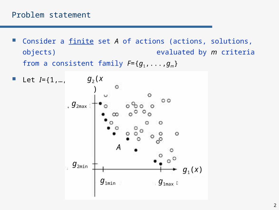
Consider a finite set A of actions (actions, solutions, objects)
evaluated by m criteria from a consistent family F={g1,...,gm}
Let I={1,…,m}
g2max
g1(x)
g2(x)
g2min
g1min g1max
A
3
What is a consistent family of criteria ?
A family of criteria F={g1,...,gn} is consistent if it is:
Complete – if two actions have the same evaluations on all criteria,
then they have to be indifferent, i.e.
if for any a,bA, there is gi(a)~gi(b), iI, then a~b
Monotonic – if action a is preferred to action b (ab), and there is
action c, such that gi(c)gi(a), iI, then cb
Non-redundant – elimination of any criterion from the family F
should violate at least one of the above properties
4
Problem statement
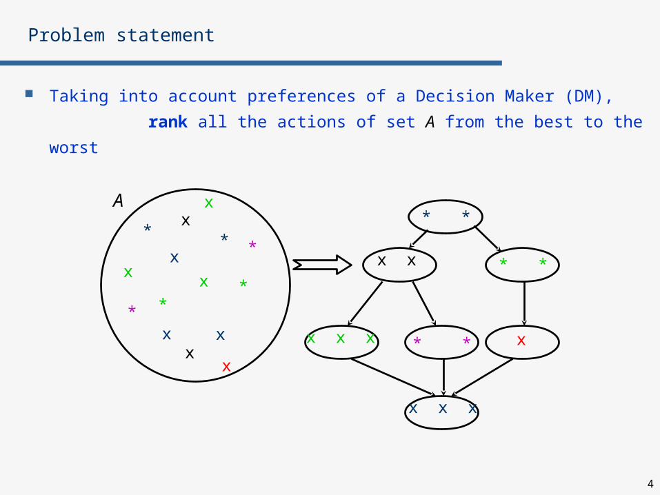
Taking into account preferences of a Decision Maker (DM),
rank all the actions of set A from the best to the worst
A
**
**
x
xx
xx
x
*
*
x
x * *
x x * *
x x x * * x
x x x
x
5
Dominance relation
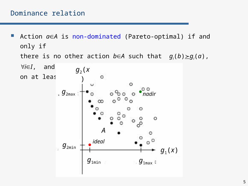
Action aA is non-dominated (Pareto-optimal) if and only if
there is no other action bA such that gi(b)gi(a), iI, and
on at least one criterion jI, gi(b)gi(a)
g2max
g1(x)
g2(x)
g2min
g1min g1max
A
ideal
nadir

6
Criteria aggregation model = preference model
Dominance relation is too poor – it leaves many actions non-comparable
One can „enrich” the dominance relation, using preference information
elicited from the Decision Maker
Preference information permits to built a preference model that
aggregates the vector evaluations of elements of A

7
Why traditional MCDM methods may confuse their users ?
Traditional MCDM methods require a rich and difficult preference information:
many intracriteria and intercriteria parameters: thresholds, weights, …
complete set of pairwise comparisons of actions on each criterion
complete set of pairwise comparisons of criteria
…
They suppose the DM understands the logic of a particular aggregation model:
meaning of weights: substitution ratios or relative strengths
meaning of lotteries (ASSESS)
meaning of indifference, preference and veto thresholds (ELECTRE)
meaning of the ratio scale of the intensity of preference (AHP)
meaning of „neutral” and „good” levels on particular criteria (MACBETH)
…
8
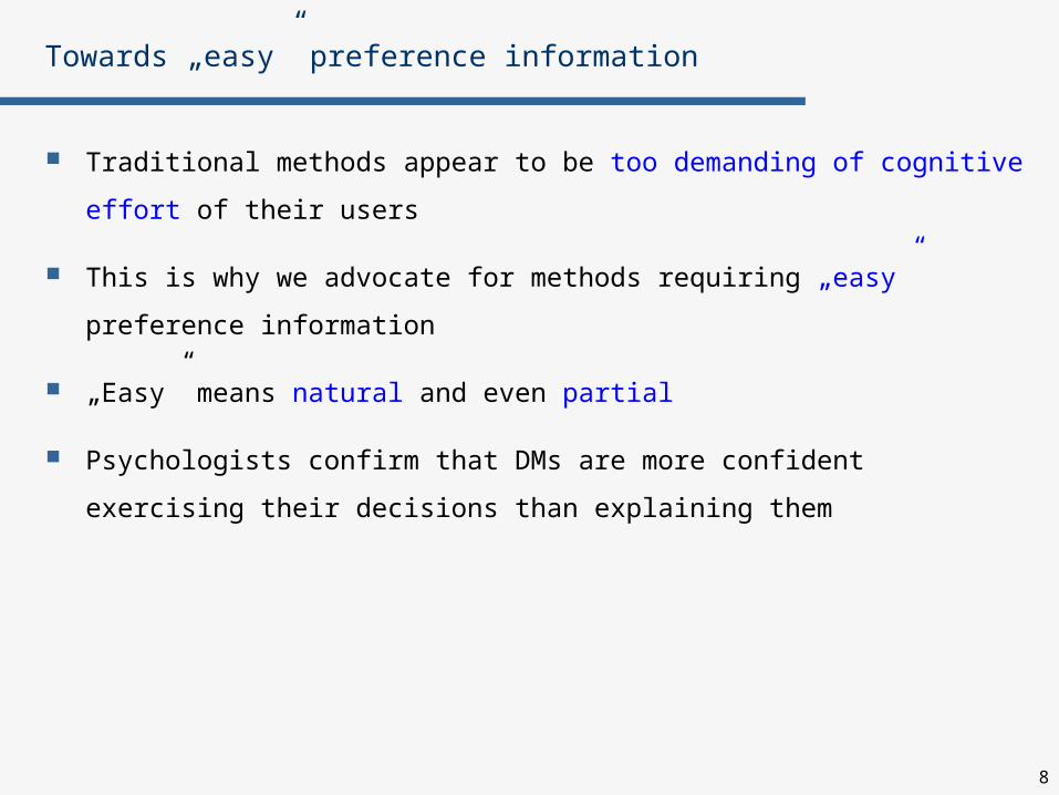
Towards „easy” preference information
Traditional methods appear to be too demanding of cognitive effort of
their users
This is why we advocate for methods requiring „easy” preference
information
„Easy” means natural and even partial
Psychologists confirm that DMs are more confident exercising their
decisions than explaining them
9
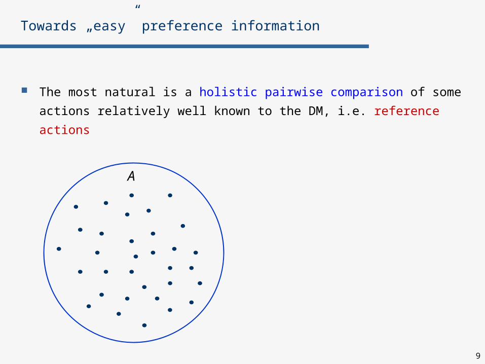
Towards „easy” preference information
The most natural is a holistic pairwise comparison of some actions
relatively well known to the DM, i.e. reference actions
A
10
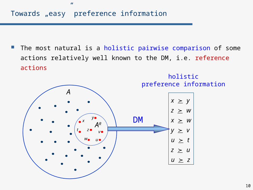
Towards „easy” preference information
The most natural is a holistic pairwise comparison of some actions
relatively well known to the DM, i.e. reference actions
A
ARx
t z
w
v
y
u
DM
x y
z w
x w
y v
u t
z u
u z
holisticpreference information
11
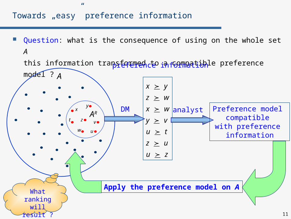
Towards „easy” preference information
Question: what is the consequence of using on the whole set A
this information transformed to a compatible preference model ?
A
ARx
t z
w
v
y
u
DM
x y
z w
x w
y v
u t
z u
u z
preference information
analyst Preference model compatible
with preference information
Apply the preference model on AWhat
ranking will
result ?
12
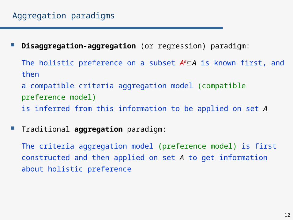
Aggregation paradigms
Disaggregation-aggregation (or regression) paradigm:
The holistic preference on a subset ARA is known first, and then
a compatible criteria aggregation model (compatible preference model)
is inferred from this information to be applied on set A
Traditional aggregation paradigm:
The criteria aggregation model (preference model) is first constructed
and then applied on set A to get information about holistic preference

13
Aggregation paradigms
The disaggregation-aggregation paradigam has been introduced
to MCDS by Jacquet-Lagreze & Siskos (1982) in the UTA method:
the inferred criteria aggregation
model is the additive value function with piecewise-linear marginal
value functions
The disaggregation-aggregation paradigam is consistent with the
„posterior rationality” principle by March (1988) and
„learning from examples” used in AI and knowledge discovery
Other aggregation models inferred in this way:
Fishburn (1967) – trade-off weights
Mousseau & Słowiński (1998) – outranking relation (ELECTRE TRI)
Greco, Matarazzo & Słowiński (1999) – decision rules or trees (DRSA – Dominance-based Rough Set Approach)
14
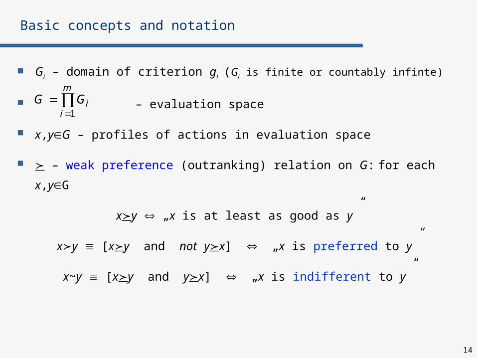
Basic concepts and notation
Gi – domain of criterion gi (Gi is finite or countably infinte)
– evaluation space
x,yG – profiles of actions in evaluation space
– weak preference (outranking) relation on G: for each x,yG
xy „x is at least as good as y”
xy [xy and not yx] „x is preferred to y”
x~y [xy and yx] „x is indifferent to y”
m
iiGG
1

15
Reminder of the UTA method (Jacquet-Lagreze & Siskos, 1982)
For simplicity: Gi , iI, where I={1,…,m}
For each gi, Gi=[i, i] is the criterion evaluation scale, i i ,
where i and i, are the worst and the best (finite) evaluations, resp.
Thus, A is a finite subset of G and
Additive value (or utility) function on G: for each xG
where ui are non-decreasing marginal value functions, ui : Gi , iI
m
iii xguxU
1
Gx,...,xxg,...,xgAx,A:g mmiii 11 , and
16
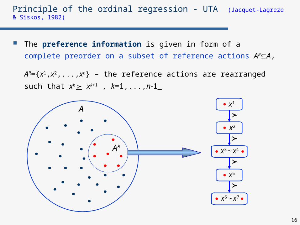
The preference information is given in form of a complete
preorder on a subset of reference actions ARA,
AR={x1,x2,...,xn} – the reference actions are rearranged such that
xk xk+1 , k=1,...,n-1
Principle of the ordinal regression - UTA (Jacquet-Lagreze & Siskos, 1982)
A
AR
x1
x2
x5
x6x7
x3x4

17
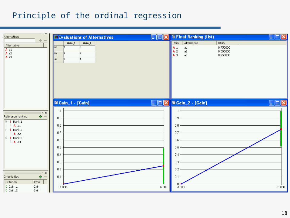
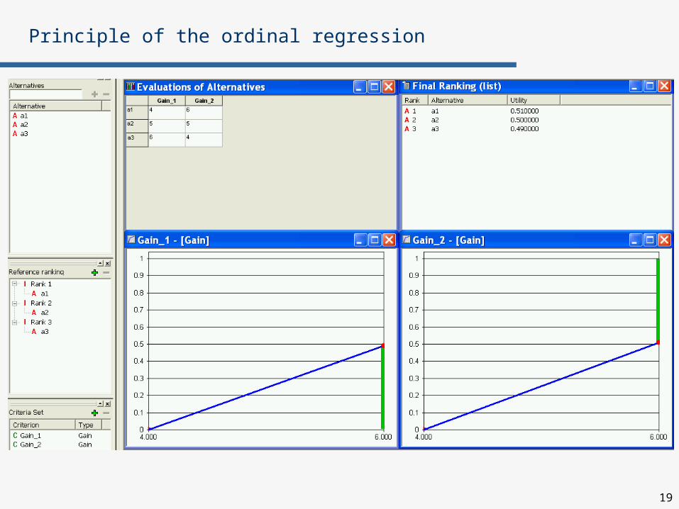
Example:
Let AR={a1, a2, a3}, G={Gain_1, Gain_2}
Evaluation of reference actions on criteria Gain_1, Gain_2:
Reference ranking:
Principle of the ordinal regression
Gain_1 Gain_2
a1 4 6
a2 5 5
a3 6 4
a1
a2
a3
18
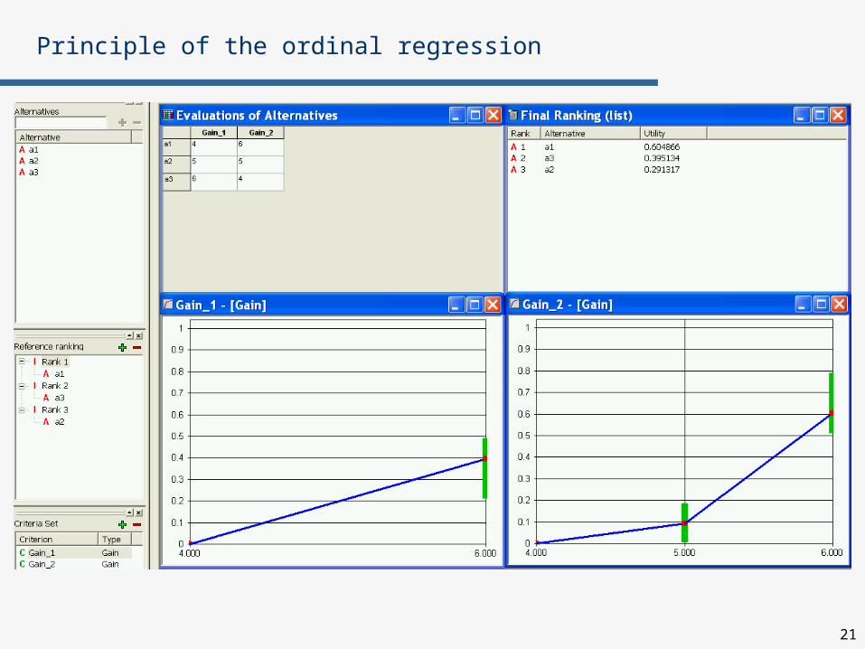
Principle of the ordinal regression
19
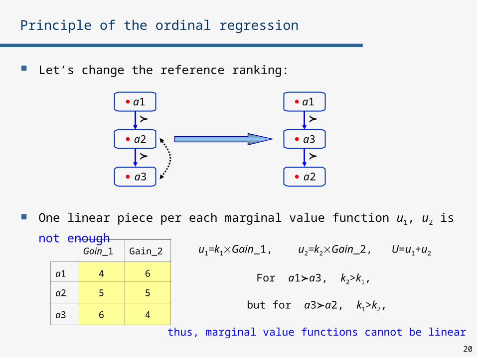
Principle of the ordinal regression
20
Let’s change the reference ranking:
One linear piece per each marginal value function u1, u2 is not enough
Principle of the ordinal regression
Gain_1 Gain_2
a1 4 6
a2 5 5
a3 6 4
a1
a3
a2
a1
a2
a3
u1=k1Gain_1, u2=k2Gain_2, U=u1+u2
For a1a3, k2>k1,
but for a3a2, k1>k2,
thus, marginal value functions cannot be linear
21
Principle of the ordinal regression

22
xxxguxg'Um
iii
1
The comprehensive preference information is given in form of
a complete preorder on a subset of reference actions ARA,
AR={x1,x2,...,xn} – the reference actions are rearranged such that
xk xk+1 , k=1,...,n-1
The inferred value of each reference action xAR
where
+ and - are potential errors of over- and under-estimation of the
right value, resp.
The intervals [i, i] are divided into i equal sub-intervals
with the end points (iI)
Principle of the UTA method (Jacquet-Lagreze & Siskos, 1982)
iiii
iji ,...,j,
jx
0 11
23
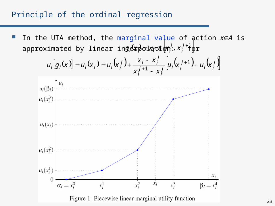
Principle of the ordinal regression
In the UTA method, the marginal value of action xA is approximated
by linear interpolation: for 1 ji
jiii x,xxxg
jii
jiij
iji
jiij
iiiiii xuxuxx
xxxuxuxgu
1
1

24
UTA additive preference model
25
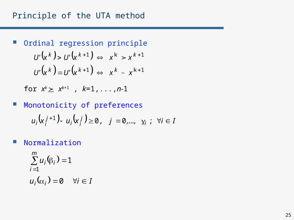
Ordinal regression principle
for xk xk+1 , k=1,...,n-1
Monotonicity of preferences
Normalization
Principle of the UTA method
1k
1
1k1
xxxU'xU'
xxxU'xU'
~kkk
kkk
Ii,...,jxuxu ijii
jii ; 0 ,01
Iiu
u
ii
m
iii
0
11

26
Principle of the UTA method
The marginal value functions (breakpoint variables) are estimated by solving the LP problem
where is a small positive constant
Ii,...,jxuxu ijii
jii ; 0 01
ji,Ax,x,x,xu
Iiu
u
Rkkkjii
ii
m
iii
and 0 0 0
0
11
(C)
1
1
11
to subject
Min
k~kkk
kkkk
Ax
kkUTA
xxxU'xU'
xxxU'xU'
xxERk
k=1,...,n-1
27
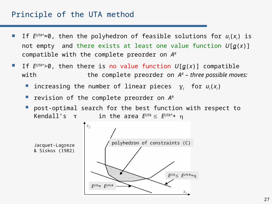
Principle of the UTA method
If EUTA*=0, then the polyhedron of feasible solutions for ui(xi) is not empty
and there exists at least one value function U[g(x)] compatible with the complete preorder on AR
If EUTA*>0, then there is no value function U[g(x)] compatible with the complete preorder on AR – three possible moves:
increasing the number of linear pieces i for ui(xi)
revision of the complete preorder on AR
post-optimal search for the best function with respect to Kendall’s in the area EUTA EUTA*+
Jacquet-Lagreze & Siskos (1982)
EUTA EUTA*+
polyhedron of constraints (C)
EUTA= EUTA*

28
Współczynnik Kendalla
Do wyznaczania odległości między preporządkami stosuje się miarę Kendalla
Przyjmijmy, że mamy dwie macierze kwadratowe R i R* o rozmiarze m m, gdzie m = |AR|, czyli m jest liczbą wariantów referencyjnych
macierz R jest związana z porządkiem referencyjnym podanym przez decydenta,
macierz R* jest związana z porządkiem dokonanym przez funkcję użyteczności wyznaczoną z zadania PL (zadania regresji porządkowej)
Każdy element macierzy R, czyli rij (i, j=1,..,m), może przyjmować wartości:
To samo dotyczy elementów macierzy R*
Tak więc w każdej z tych macierzy kodujemy pozycję (w porządku) wariantu a względem wariantu b
gdy ,1
gdy ,50
gdy ,0
ji
i~j
ij
ij
aa
aa.
aalubji
r

29
Współczynnik Kendalla
Następnie oblicza się współczynnik Kendalla :
gdzie dk(R,R*) jest odległością Kendalla między macierzami R i R*:
Stąd -1, 1
Jeżeli = -1, to oznacza to, że porządki zakodowane w macierzach R i R*
są zupełnie odwrotne, np. macierz R koduje porządek a b c d,
a macierz R* porządek d c b a
Jeżeli = 1, to zachodzi całkowita zgodność porządków z obydwu macierzy.
W tej sytuacji błąd estymacji funkcji użyteczności F*=0
W praktyce funkcję użyteczności akceptuje się, gdy 0.75
1
41
mm
*R,Rdk
m
i
m
jijijk *rr*R,Rd
1 121
30
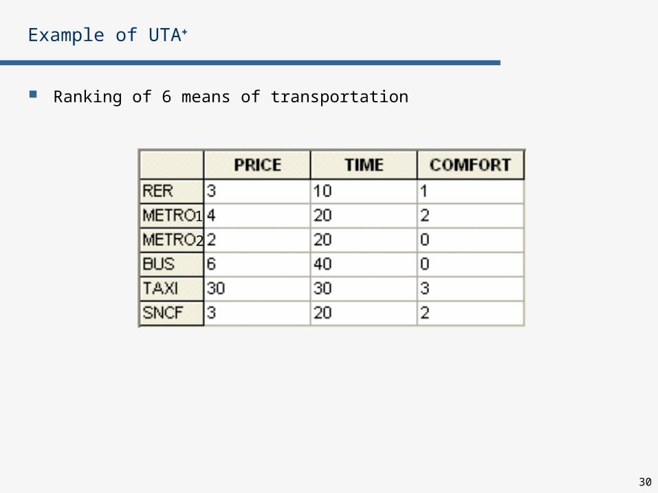
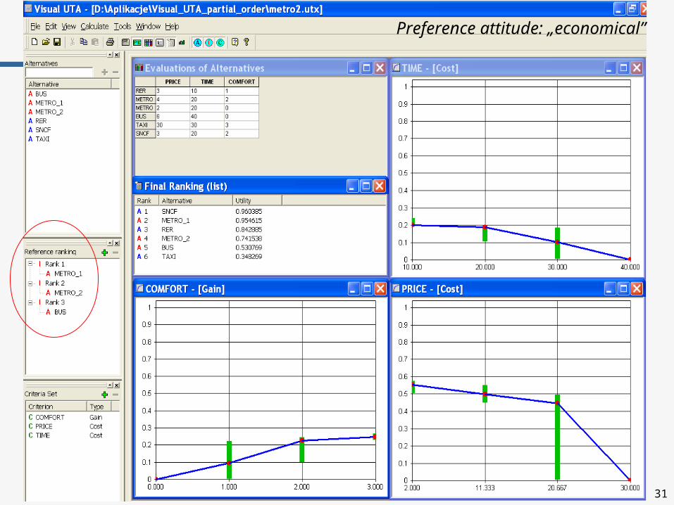
Example of UTA+
Ranking of 6 means of transportation
1
2
31
Preference attitude: „economical”
32
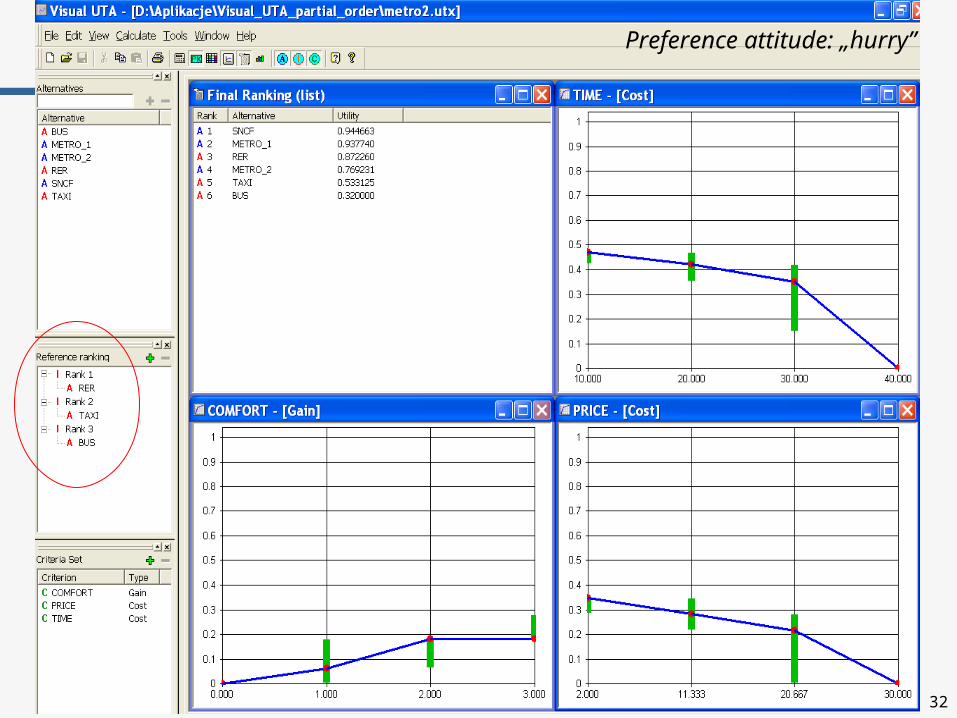
Preference attitude: „hurry”
33
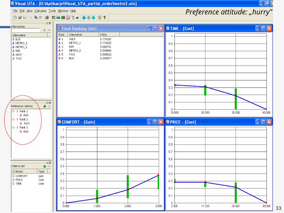
Preference attitude: „hurry”
34
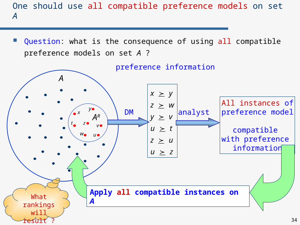
One should use all compatible preference models on set A
Question: what is the consequence of using all compatible preference
models on set A ?
A
ARx
t z
w
v
y
u
DM
x y
z w
y v
u t
z u
u z
preference information
analystAll instances of
preference model compatible
with preference information
What rankings
will result ?
Apply all compatible instances on A
35
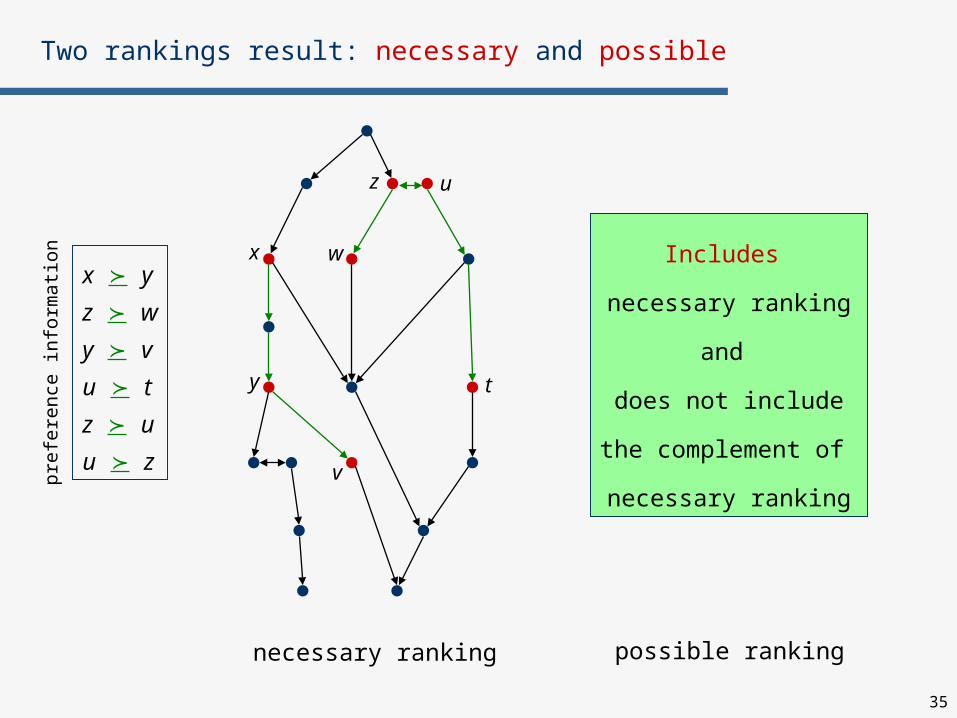
Two rankings result: necessary and possible
x
y
w
z
t
u
v
necessary ranking possible ranking
Includes
necessary ranking
and
does not include
the complement of
necessary ranking
x y
z w
y v
u t
z u
u zpre
fere
nce
info
rmati
on
36
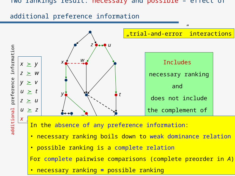
Two rankings result: necessary and possible – effect of additional preference information
possible rankingimpoverished
Includes
necessary ranking
and
does not include
the complement of
necessary ranking
x y
z w
y v
u t
z u
u z
x w
addit
ion
al pre
fere
nce
info
rmati
on
x
y
w
z
t
u
v
necessary rankingenriched
„trial-and-error” interactions
In the absence of any preference information:
• necessary ranking boils down to weak dominance relation
• possible ranking is a complete relation
For complete pairwise comparisons (complete preorder in A):
• necessary ranking = possible ranking
37
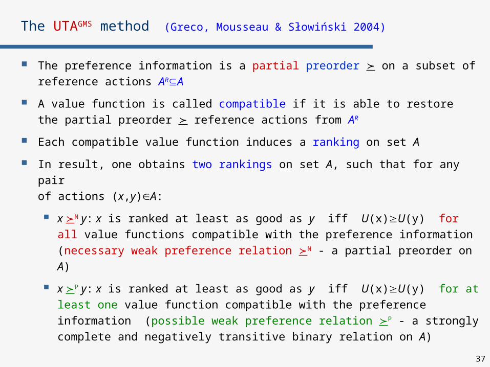
The UTAGMS method (Greco, Mousseau & Słowiński 2004)
The preference information is a partial preorder on a subset of reference actions ARA
A value function is called compatible if it is able to restore the partial preorder reference actions from AR
Each compatible value function induces a ranking on set A
In result, one obtains two rankings on set A, such that for any pair of actions (x,y)A:
x N y: x is ranked at least as good as y iff U(x)U(y) for all value functions compatible with the preference information (necessary weak preference relation N - a partial preorder on A)
x P y: x is ranked at least as good as y iff U(x)U(y) for at least one value function compatible with the preference information (possible weak preference relation P - a strongly complete and negatively transitive binary relation on A)
38
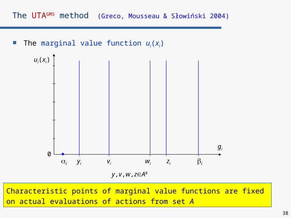
The UTAGMS method (Greco, Mousseau & Słowiński 2004)
The marginal value function ui(xi)
ui(xi)
gi
0i yi iwi zivi
y,v,w,zAR
Characteristic points of marginal value functions are fixed on actual evaluations of actions from set A

39
The UTAGMS method (Greco, Mousseau & Słowiński 2004)
The marginal value function ui(xi)
ui(xi)
gi
0i yi iwi zivi
??
?
??
y,v,w,zAR
Marginal values in characteristic points are unknown

40
The UTAGMS method (Greco, Mousseau & Słowiński 2004)
The marginal value function ui(xi)
ui(xi)
gi
0i yi iwi zivi
y,v,w,zAR
In fact, they are intervals, because all compatible value functions are considered
41
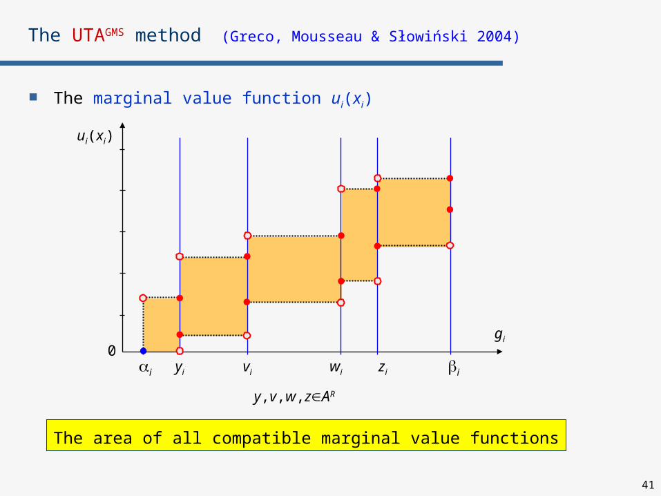
The UTAGMS method (Greco, Mousseau & Słowiński 2004)
The marginal value function ui(xi)
ui(xi)
gi
0i yi iwi zivi
y,v,w,zAR
The area of all compatible marginal value functions
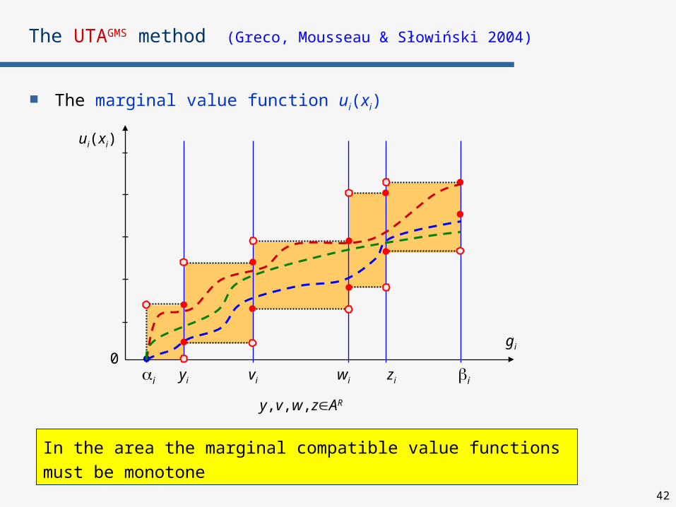
42
The UTAGMS method (Greco, Mousseau & Słowiński 2004)
The marginal value function ui(xi)
ui(xi)
gi
0i yi iwi zivi
y,v,w,zAR
In the area the marginal compatible value functions must be monotone
43
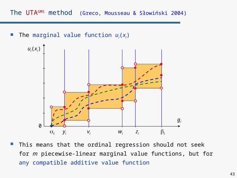
The UTAGMS method (Greco, Mousseau & Słowiński 2004)
The marginal value function ui(xi)
This means that the ordinal regression should not seek
for m piecewise-linear marginal value functions, but for
any compatible additive value function
ui(xi)
gi
0i yi iwi zivi
44
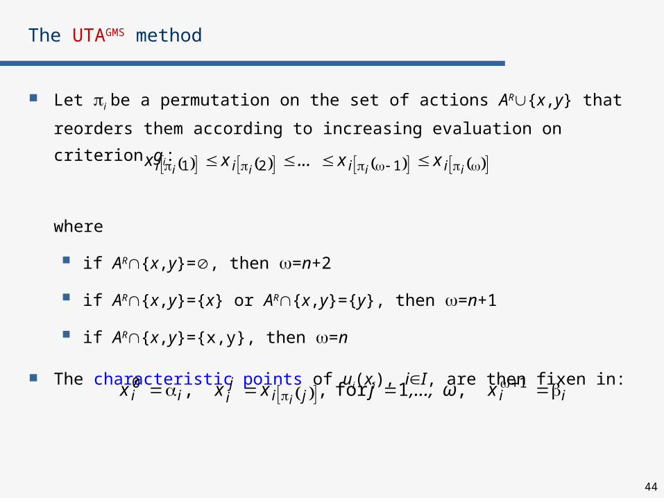
The UTAGMS method
Let i be a permutation on the set of actions AR{x,y} that reorders
them according to increasing evaluation on criterion gi:
where
if AR{x,y}=, then =n+2
if AR{x,y}={x} or AR{x,y}={y}, then =n+1
if AR{x,y}={x,y}, then =n
The characteristic points of ui(xi), iI, are then fixen in:
iiii iiii xx...xx 121
iijijiii x,..., ωjxxx
i
10 ,1for , ,
45
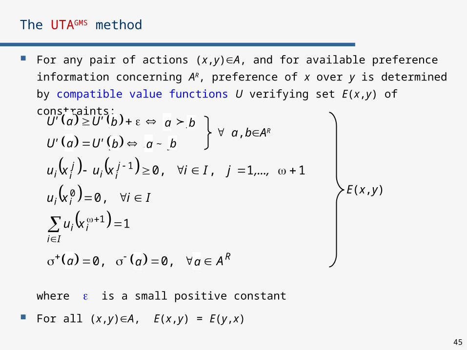
The UTAGMS method
For any pair of actions (x,y)A, and for available preference
information concerning AR, preference of x over y is determined
by compatible value functions U verifying set E(x,y) of constraints:
where is a small positive constant
For all (x,y)A, E(x,y) = E(y,x)
R
Iiii
ii
jii
jii
~
Axxx
xu
Iixu
,...,jIixuxu
yxy'Ux'U
yxy'Ux'U
,0 ,0
1
0,
11 , ,0
1
0
1
a,bAR
E(x,y)
a
b
b
b
b
a
aaa
a
a
46
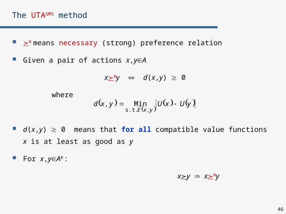
N means necessary (strong) preference relation
Given a pair of actions x,yA
xNy d(x,y) 0
where
d(x,y) 0 means that for all compatible value functions
x is at least as good as y
For x,yAR :
xy xNy
The UTAGMS method
yUxUy,xdy,xE
s.t.Min
47
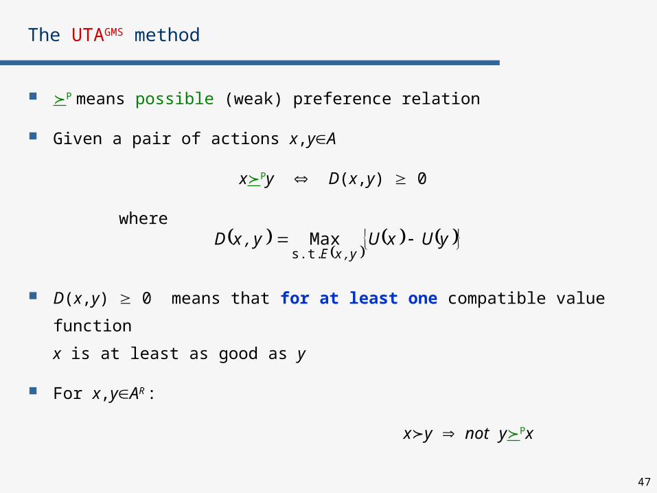
P means possible (weak) preference relation
Given a pair of actions x,yA
xPy D(x,y) 0
where
D(x,y) 0 means that for at least one compatible value function
x is at least as good as y
For x,yAR :
xy not yPx
The UTAGMS method
yUxUy,xDy,xE
s.t.Max
48
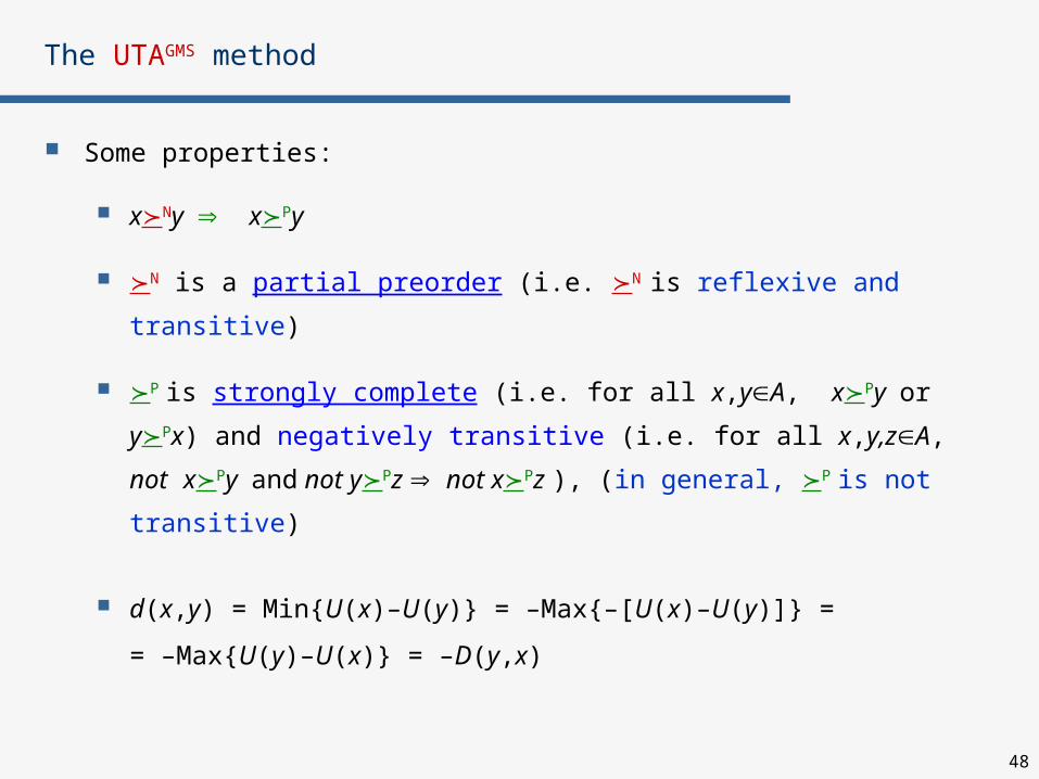
Some properties:
xNy xPy
N is a partial preorder (i.e. N is reflexive and transitive)
P is strongly complete (i.e. for all x,yA, xPy or yPx) and
negatively transitive (i.e. for all x,y,zA, not xPy and not yPz
not xPz ), (in general, P is not transitive)
d(x,y) = Min{U(x)–U(y)} = –Max{–[U(x)–U(y)]} =
= –Max{U(y)–U(x)} = –D(y,x)
The UTAGMS method
49
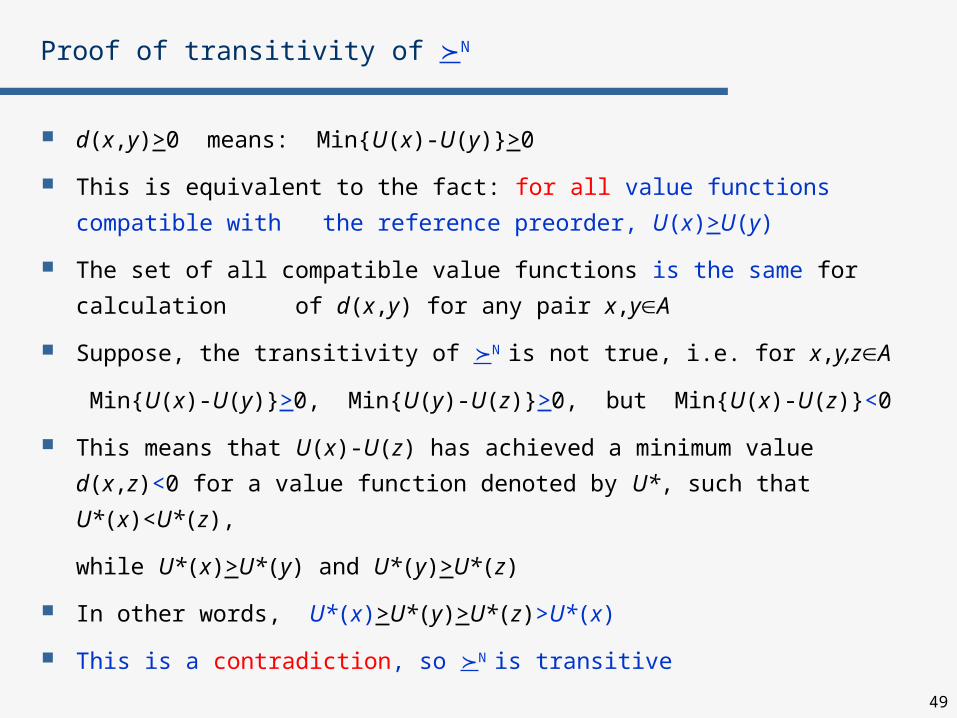
Proof of transitivity of N
d(x,y)>0 means: Min{U(x)-U(y)}>0
This is equivalent to the fact: for all value functions compatible with
the reference preorder, U(x)>U(y)
The set of all compatible value functions is the same for calculation
of d(x,y) for any pair x,yA
Suppose, the transitivity of N is not true, i.e. for x,y,zA
Min{U(x)-U(y)}>0, Min{U(y)-U(z)}>0, but Min{U(x)-U(z)}<0
This means that U(x)-U(z) has achieved a minimum value d(x,z)<0 for
a value function denoted by U*, such that U*(x)<U*(z),
while U*(x)>U*(y) and U*(y)>U*(z)
In other words, U*(x)>U*(y)>U*(z)>U*(x)
This is a contradiction, so N is transitive

50
The UTAGMS method
Elaboration of the final ranking:
for the necessary preference relation being a partial preorder
(N is supported by all compatible value functions)
preference: xNy if xNy and not yNx
indifference: xNy if xNy and yNx
incomparability: x ? y if not xNy and not yNx
for the possible preference relation being complete
(P is supported by at least one compatible value function)
preference: xPy if xPy and not yPx
indifference: xPy if xPy and yPx
N.B. It is impossible to infer one ranking from another because
strong and weak outranking relations are not dual

51
The UTAGMS method – final ranking (partial preorder)
Final ranking corresponding to necessary (strong) preference :
N
N
N
N
N
N
N
N
N
52
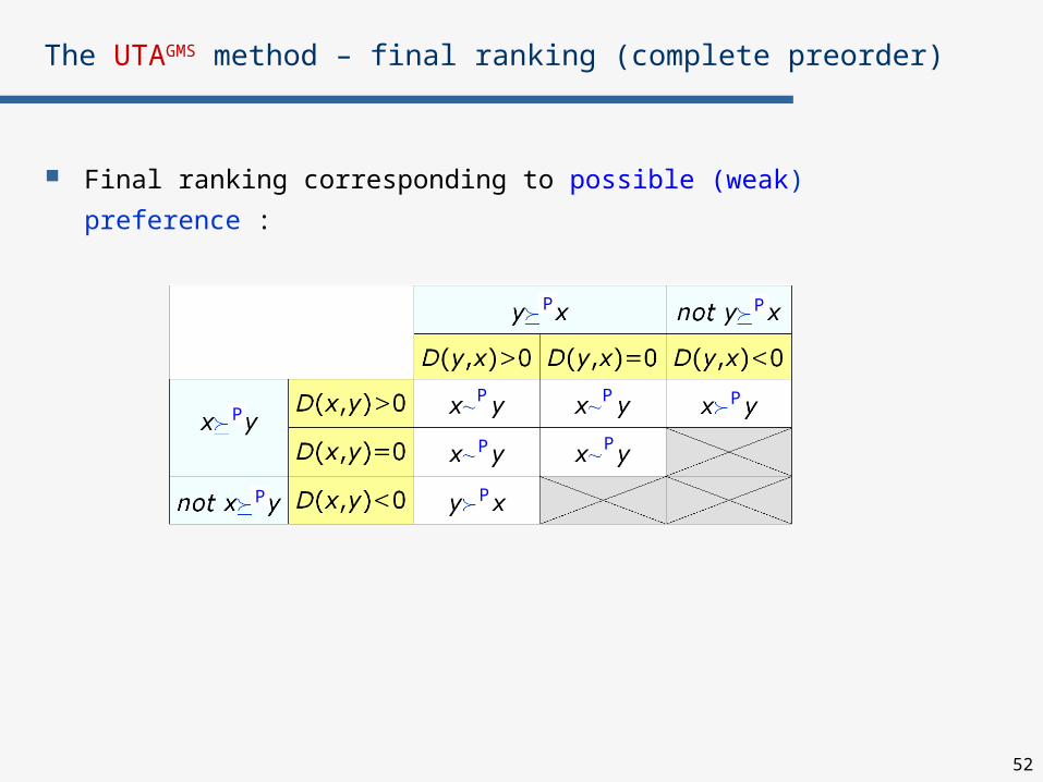
Final ranking corresponding to possible (weak) preference :
The UTAGMS method – final ranking (complete preorder)
PP
P P
PP
P
P
P
P
53
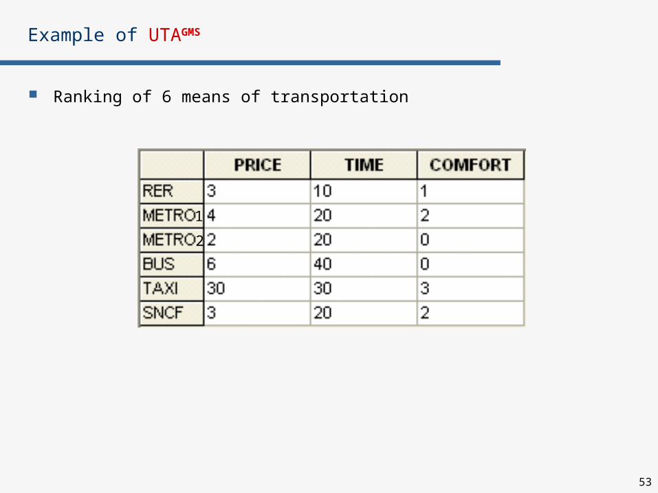
Example of UTAGMS
Ranking of 6 means of transportation
1
2
54
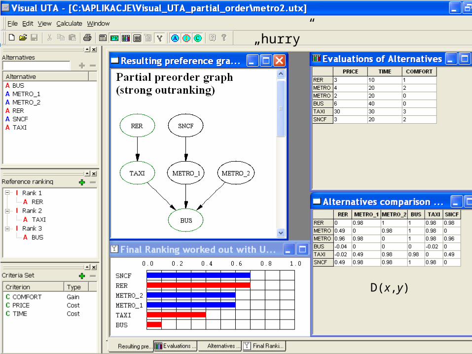
„hurry”
D(x,y)
56
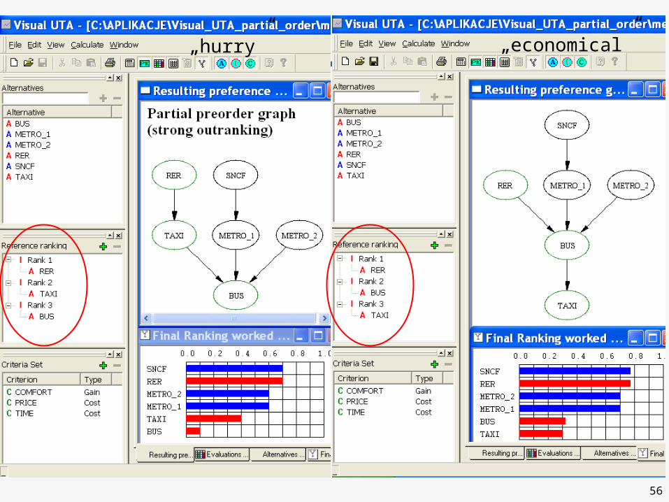
„hurry” „economical”
57
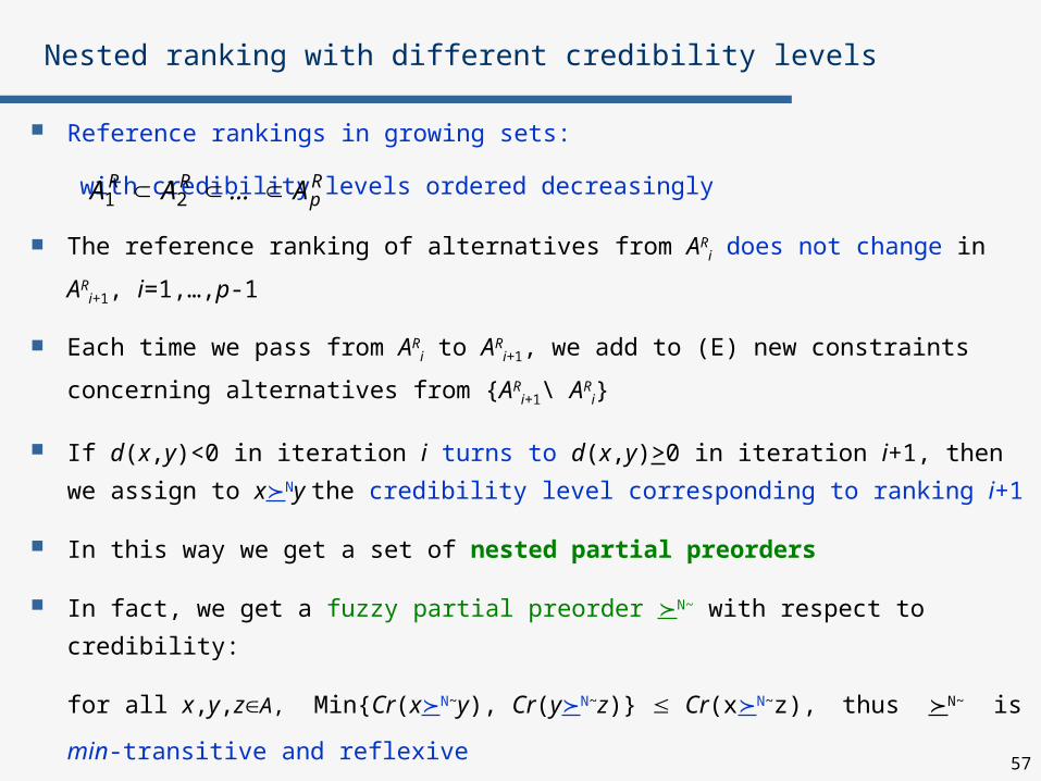
Nested ranking with different credibility levels
Reference rankings in growing sets:
with credibility levels ordered decreasingly
The reference ranking of alternatives from ARi does not change in AR
i+1,
i=1,…,p-1
Each time we pass from ARi to AR
i+1, we add to (E) new constraints
concerning alternatives from {ARi+1\ AR
i}
If d(x,y)<0 in iteration i turns to d(x,y)>0 in iteration i+1, then we assign
to xNy the credibility level corresponding to ranking i+1
In this way we get a set of nested partial preorders
In fact, we get a fuzzy partial preorder N~ with respect to credibility:
for all x,y,zA, Min{Cr(xN~y), Cr(yN~z)} Cr(xN~z),
thus N~ is min-transitive and reflexive
Rp
RR A...AA 21

58
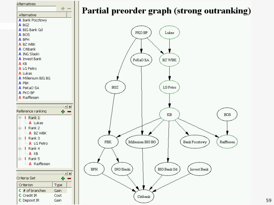
Software demonstration
Bank
59

60
New reference action
61
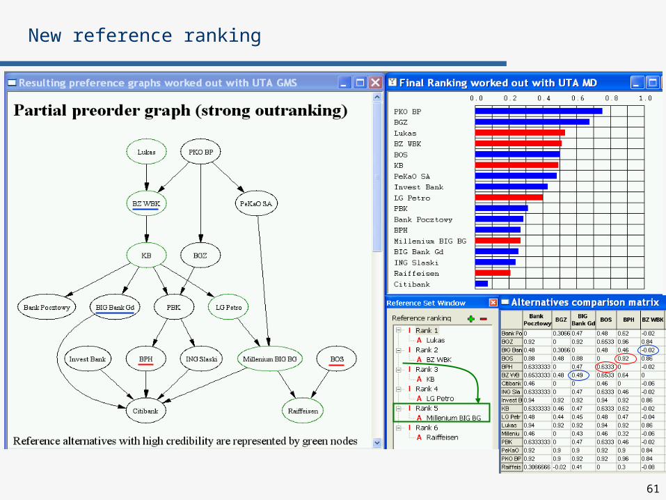
New reference ranking

62
High credibility ranking embedded in low credibility ranking
Partial preorder graph (strong outranking)

63
GRIP – Generalized Regression with Intensities of Preference (Figueira, Greco, Słowiński 2006)
GRIP extends the UTAGMS method by adopting all features of UTAGMS
and by taking into account additional preference information :
comprehensive comparisons of intensities of preference between
some pairs of reference actions,
e.g. „x is preferred to y at least as much as w is preferred to z”
partial comparisons of intensities of preference between some
pairs of reference actions on particular criteria,
e.g. „x is preferred to y at least as much as w is preferred to z, on
criterion giF”
64
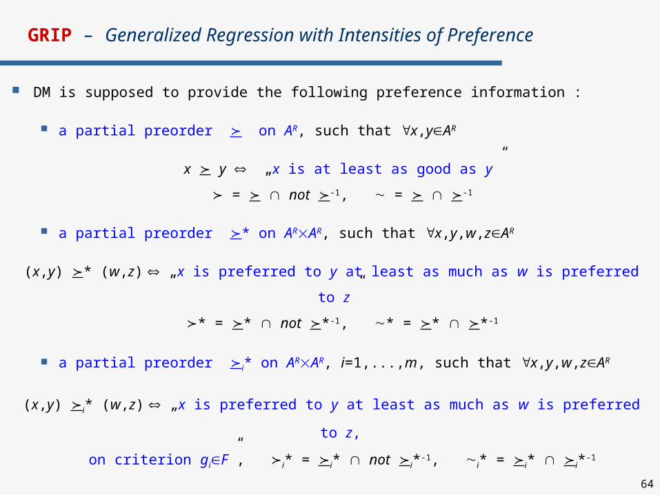
GRIP – Generalized Regression with Intensities of Preference
DM is supposed to provide the following preference information :
a partial preorder on AR, such that x,yAR
x y „x is at least as good as y”
= not -1, = -1
a partial preorder * on ARAR, such that x,y,w,zAR
(x,y) * (w,z) „x is preferred to y at least as much as w is preferred to z”
* = * not *-1, * = * *-1
a partial preorder i* on ARAR, i=1,...,m, such that x,y,w,zAR
(x,y) i* (w,z) „x is preferred to y at least as much as w is preferred to z,
on criterion giF”, i* = i* not i*-1, i* = i* i*-1
65
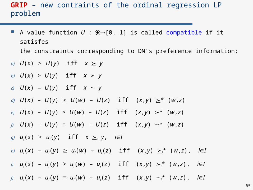
GRIP – new contraints of the ordinal regression LP problem
A value function U : [0, 1] is called compatible if it satisfes
the constraints corresponding to DM’s preference information:
a) U(x) U(y) iff x y
b) U(x) > U(y) iff x y
c) U(x) = U(y) iff x y
d) U(x) – U(y) U(w) – U(z) iff (x,y) * (w,z)
e) U(x) – U(y) > U(w) – U(z) iff (x,y) * (w,z)
f) U(x) – U(y) = U(w) – U(z) iff (x,y) * (w,z)
g) ui(x) ui(y) iff x i y, iI
h) ui(x) – ui(y) ui(w) – ui(z) iff (x,y) i* (w,z), iI
i) ui(x) – ui(y) > ui(w) – ui(z) iff (x,y) i* (w,z), iI
j) ui(x) – ui(y) = ui(w) – ui(z) iff (x,y) i* (w,z), iI
66
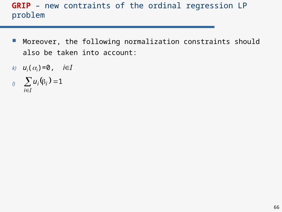
GRIP – new contraints of the ordinal regression LP problem
Moreover, the following normalization constraints should also be
taken into account:
k) ui(i)=0, iI
l) 1Ii
iiu
67
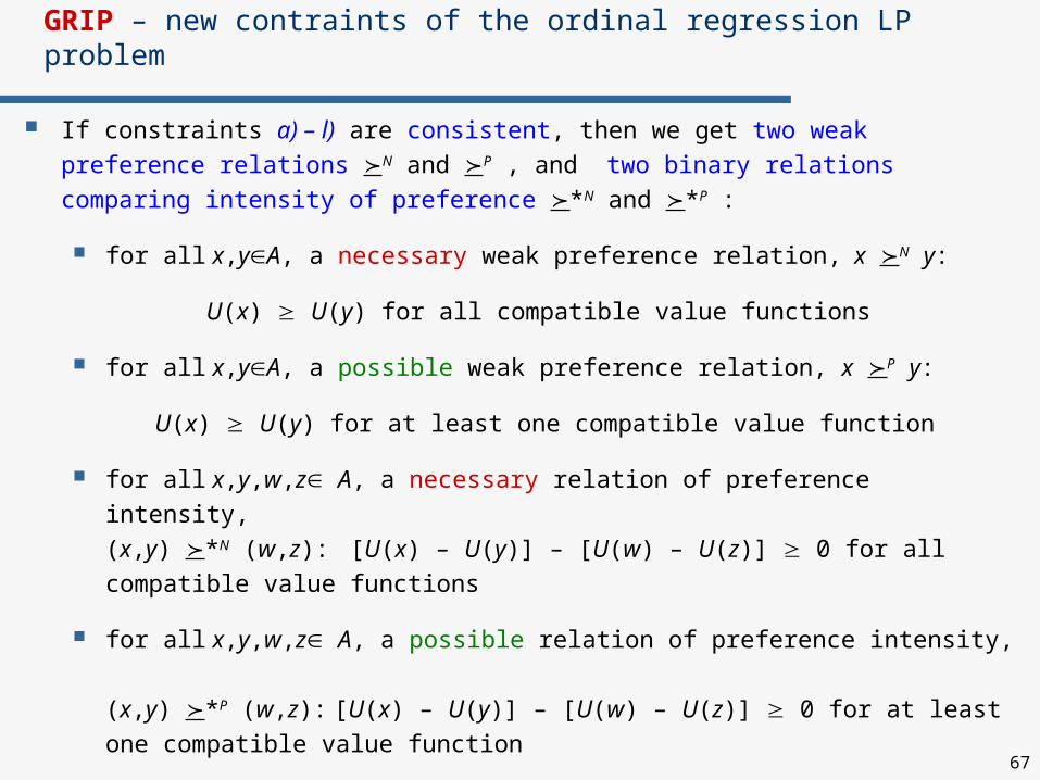
If constraints a) – l) are consistent, then we get two weak preference relations N and P , and two binary relations comparing intensity of preference *N and *P :
for all x,yA, a necessary weak preference relation, x N y:
U(x) U(y) for all compatible value functions
for all x,yA, a possible weak preference relation, x P y:
U(x) U(y) for at least one compatible value function
for all x,y,w,z A, a necessary relation of preference intensity,(x,y) *N (w,z): [U(x) – U(y)] – [U(w) – U(z)] 0 for all compatible value functions
for all x,y,w,z A, a possible relation of preference intensity, (x,y) *P (w,z): [U(x) – U(y)] – [U(w) – U(z)] 0 for at least one compatible value function
GRIP – new contraints of the ordinal regression LP problem

68
Theorem: If constaraints a) – l) are satisfied, then the properties hold:
1. For all x,yA, x N y x P y
2. For all x,yAR, x y x N y
3. N is a partial preorder (i.e. the relation is transitive and reflexive) andP is strongly complete and negatively transitive
4. For all x,y,zA, [x N y and y P z] x P z
5. For all x,y,zA, [x P y and y N z] x P z
6. For all x,y,w,zA, (x,y) *N (w,z) (x,y) *P (w,z)
7. For all x,y,w,zA, (x,y) * (w,z) (x,y) *N (w,z)
3. *N is a partial preorder and *P is strongly complete and negatively transitive
9. For all x,y,w,z,r,sA, [(x,y) *N (w,z) and (w,z) *P (r,s)] (x',y) *P (r,s)
10. For all x,y,w,z,r,sA, [(x,y) *P (w,z) and (w,z) *N (r,s)] (x,y) *P (r,s)
11. For all x,x’,y,w,zA, [x’ N x and (x,y) *N (w,z)] (x’,y) *N (w,z)
12. For all x,x’,y,w,zA, [x’ N x and (x,y) *P (w,z)] (x’,y) *P (w,z)
13. For all x,x’,y,w,zA, [x’ P x and (x,y) *N (w,z)] (x’,y) *P (w,z)
GRIP – fundamental properties of N, P, *N, *P

69
14. For all x,y,y’,w,zA, [y N y’ and (x,y) *N (w,z)] (x,y’) *N (w,z)
15. For all x,y,y’,w,zA, [y N y’ and (x,y) *P (w,z)] (x,y’) *P (w,z)
16. For all x,y,y’,w,zA, [y P y’ and (x,y) *N (w,z)] (x,y’) *P (w,z)
17. For all x,y,w,w’,zA, [w N w’ and (x,y) *N (w,z)] (x,y) *N (w’,z)
18. For all x,y,w,w’,zA, [w N w’ and (x,y) *P (w,z)] (x,y) *P (w’,z)
19. For all x,y,w,w’,zA, [w P w’ and (x,y) *N (w,z)] (x,y) *P (w’,z)
20. For all x,y,w,z,z’A, [z’ N z and (x,y) *N (w,z)] (x,y) *N (w,z’)
21. For all x,y,w,z,z’A, [z’ N z and (x,y) *P (w,z)] (x,y) *P (w,z’)
22. For all x,y,w,z,z’A, [z’ P z and (x,y) *N (w,z)] (x,y) *P (w,z’)
23. For all x,x’,yA, (x’,y) *N (x,y) x’ N x
24. For all x,x’,yA, (x’,y) *P (x,y) x’ P x
25. For all x,y,y’A, (x,y) *N (x,y’) y’ N y
26. For all x,y,y’A, (x,y) *P (x,y’) y’ P y
GRIP – fundamental properties of N, P, *N, *P
70
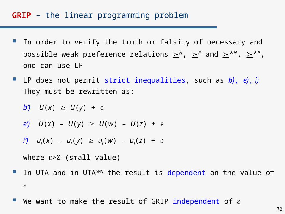
GRIP – the linear programming problem
In order to verify the truth or falsity of necessary and possible weak
preference relations N, P and *N, *P, one can use LP
LP does not permit strict inequalities, such as b), e), i)
They must be rewritten as:
b’) U(x) U(y) +
e’) U(x) – U(y) U(w) – U(z) +
i’) ui(x) – ui(y) ui(w) – ui(z) +
where >0 (small value)
In UTA and in UTAGMS the result is dependent on the value of
We want to make the result of GRIP independent of
71
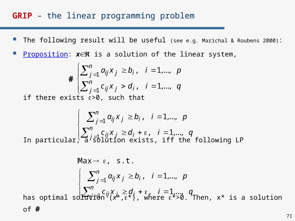
GRIP – the linear programming problem
The following result will be useful (see e.g. Marichal & Roubens 2000):
Proposition: x is a solution of the linear system,
if there exists >0, such that
In particular, a solution exists, iff the following LP
has optimal solution (x*,*), where *>0. Then, x* is a solution of #
nj ijij
nj ijij
q,...,idxc
p,...,ibxa
1
1
1 ,
1 ,
nj ijij
nj ijij
q,...,idxc
p,...,ibxa
1
1
1 ,
1 ,#
nj ijij
nj ijij
q,...,idxc
p,...,ibxa
1
1
1 ,
1 ,
s.t. ,MinMax
72
GRIP – the linear programming problem
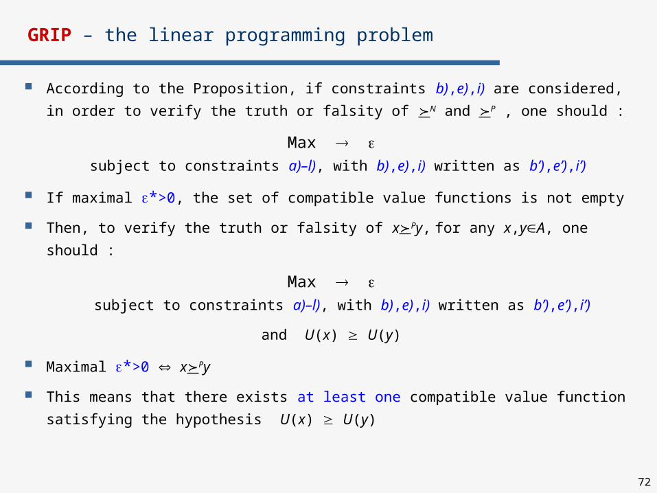
According to the Proposition, if constraints b),e),i) are considered,
in order to verify the truth or falsity of N and P , one should :
Max subject to constraints a)–l), with b),e),i) written as b’),e’),i’)
If maximal *>0, the set of compatible value functions is not empty
Then, to verify the truth or falsity of xPy, for any x,yA, one should :
Max subject to constraints a)–l), with b),e),i) written as b’),e’),i’)
and U(x) U(y)
Maximal *>0 xPy
This means that there exists at least one compatible value function
satisfying the hypothesis U(x) U(y)
73
GRIP – the linear programming problem
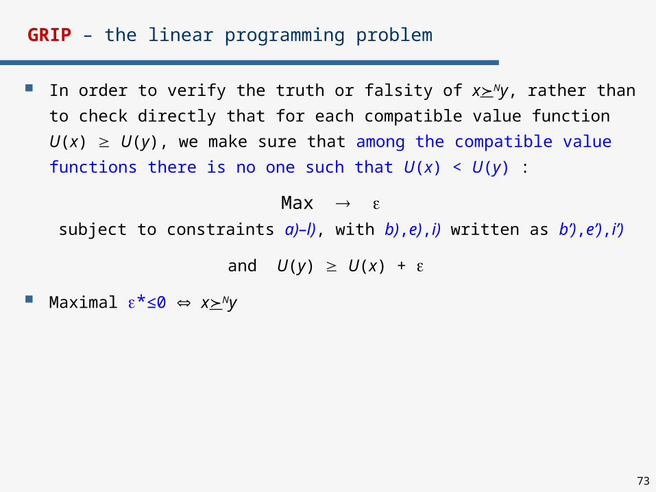
In order to verify the truth or falsity of xNy, rather than to check
directly that for each compatible value function U(x) U(y), we make
sure that among the compatible value functions there is no one such
that U(x) < U(y) :
Max subject to constraints a)–l), with b),e),i) written as b’),e’),i’)
and U(y) U(x) +
Maximal *≤0 xNy
74
GRIP – the linear programming problem
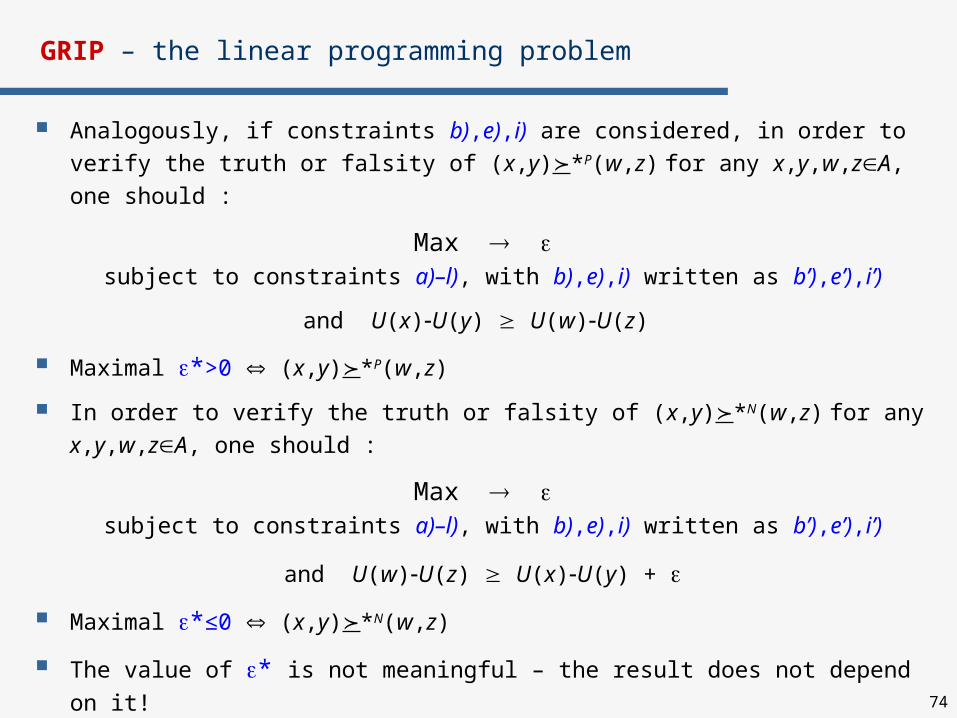
Analogously, if constraints b),e),i) are considered, in order to verify the truth or falsity of (x,y)*P(w,z) for any x,y,w,zA, one should :
Max subject to constraints a)–l), with b),e),i) written as b’),e’),i’)
and U(x)U(y) U(w)U(z)
Maximal *>0 (x,y)*P(w,z)
In order to verify the truth or falsity of (x,y)*N(w,z) for any x,y,w,zA, one should :
Max subject to constraints a)–l), with b),e),i) written as b’),e’),i’)
and U(w)U(z) U(x)U(y) +
Maximal *≤0 (x,y)*N(w,z)
The value of * is not meaningful – the result does not depend on it!

75
Comparison of GRIP and MACBETH (Bana e Costa & Vansnick 1994)
MACBETH
• Ordinal preference inf. w.r.t. each criterion for all not equally attractive pairs of actions: xiy or yix, x,yA
• Definition of „neutral” and „good” level on original scales of criteria
• Absolute qualitative judgement of differences of attractiveness for all not equally attractive pairs of actions w.r.t. each criterion, including „good” and „neutral” points (e.g. v_weak, weak, moderate,..., extreme int.pref. for (x,y))
• Ordinal preference inf. for all not equally attractive criteria: gigj or gjgi
• Absolute qualitative judgement of differences of attractiveness for all not equally attractive pairs of criteria (e.g. v_weak, weak, moderate,..., extreme intensity of preference for (gi,gj))
GRIP
• Ordinal comprehensive preference inf. on pairwise comparison of some
reference actions: xy, x,yAR
• Absolute qualitative judgement of intensity of preference for some pairs of reference actions – partial and/or comprehensive (e.g. v_weak, weak, moderate,..., extreme intensity of preference for (x,y))
OR• Comparison of intensities of preference for some pairs of reference actions – partial and/or comprehens.: (x,y)i(w,z) and/or (x,y)(w,z)
Pre
fere
nce
info
rmati
on
76
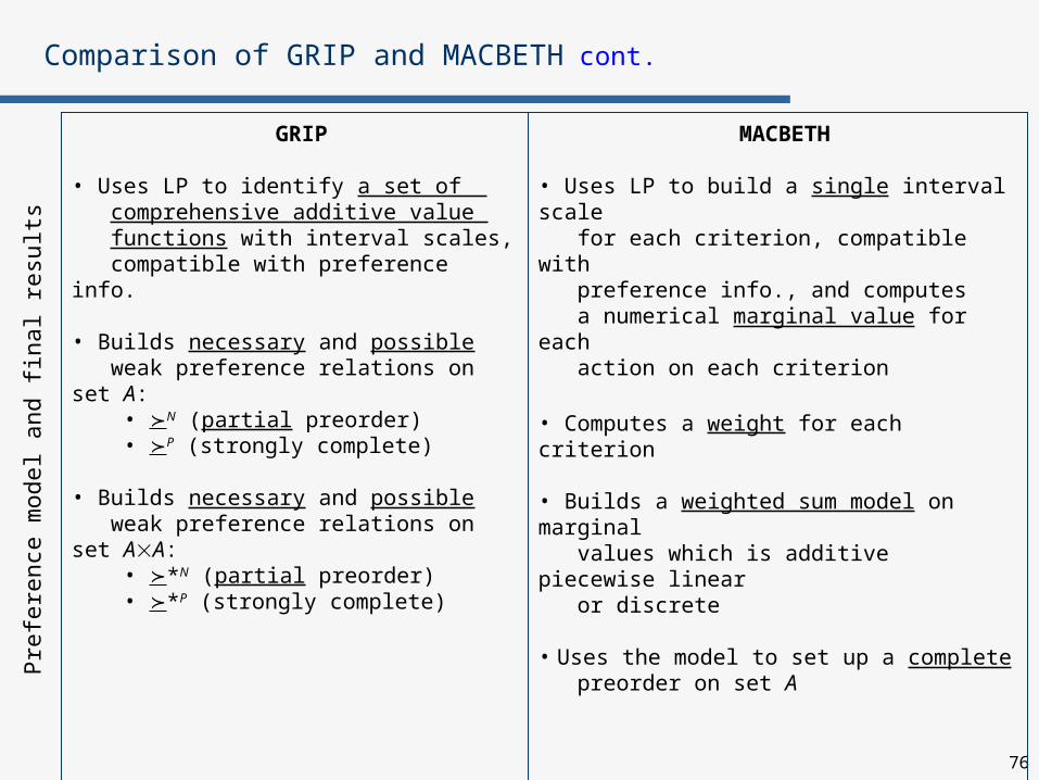
Comparison of GRIP and MACBETH cont.
MACBETH
• Uses LP to build a single interval scale for each criterion, compatible with preference info., and computes a numerical marginal value for each action on each criterion
• Computes a weight for each criterion
• Builds a weighted sum model on marginal values which is additive piecewise linear or discrete
• Uses the model to set up a complete preorder on set A
GRIP
• Uses LP to identify a set of comprehensive additive value functions with interval scales, compatible with preference info.
• Builds necessary and possible weak preference relations on set A:
• N (partial preorder)• P (strongly complete)
• Builds necessary and possible weak preference relations on set AA:
• *N (partial preorder) • *P (strongly complete)
Pre
fere
nce
model and fi
nal re
sult
s
77
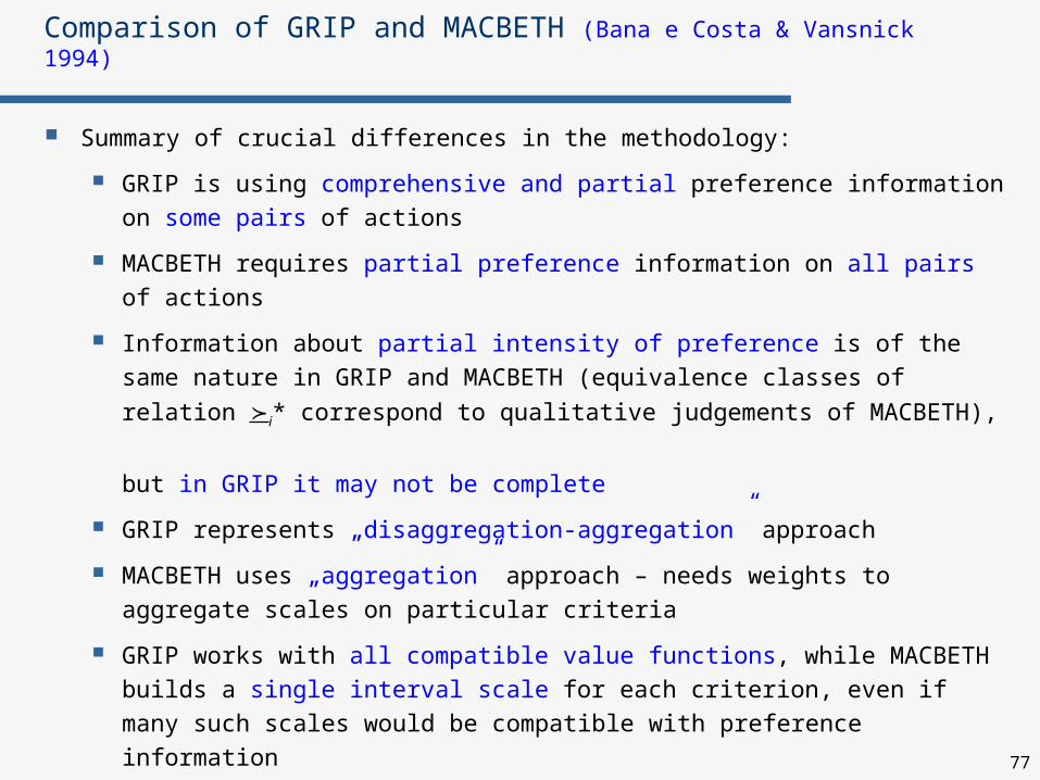
Comparison of GRIP and MACBETH (Bana e Costa & Vansnick 1994)
Summary of crucial differences in the methodology:
GRIP is using comprehensive and partial preference information on some pairs of actions
MACBETH requires partial preference information on all pairs of actions
Information about partial intensity of preference is of the same
nature in GRIP and MACBETH (equivalence classes of relation i*
correspond to qualitative judgements of MACBETH), but in GRIP it may not be complete
GRIP represents „disaggregation-aggregation” approach
MACBETH uses „aggregation” approach – needs weights to aggregate scales on particular criteria
GRIP works with all compatible value functions, while MACBETH builds a single interval scale for each criterion, even if many such scales would be compatible with preference information
78
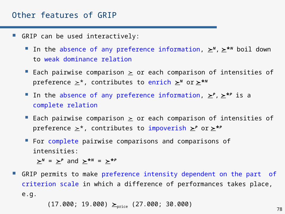
Other features of GRIP
GRIP can be used interactively:
In the absence of any preference information, N, *N boil down to
weak dominance relation
Each pairwise comparison or each comparison of intensities of
preference *, contributes to enrich N or *N
In the absence of any preference information, P, *P is a
complete relation
Each pairwise comparison or each comparison of intensities of
preference *, contributes to impoverish P or *P
For complete pairwise comparisons and comparisons of intensities:
N = P and *N = *P
GRIP permits to make preference intensity dependent on the part of
criterion scale in which a difference of performances takes place, e.g.
(17.000; 19.000) price (27.000; 30.000)
79
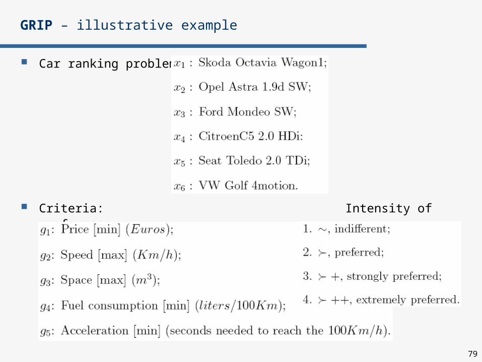
GRIP – illustrative example
Car ranking problem
Criteria: Intensity of preference:

80
GRIP – illustrative example
Performance matrix
Skoda
Opel
Ford
Citroen
Seat
VW
Price Speed Space Fuel_cons. Acceleration
81
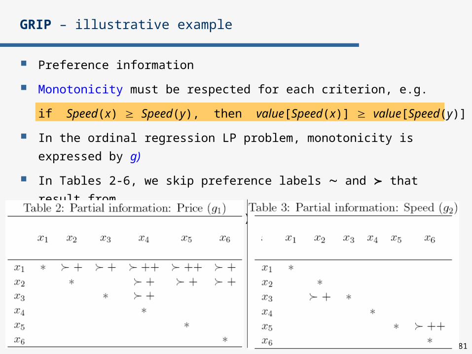
Preference information
Monotonicity must be respected for each criterion, e.g.
if Speed(x) Speed(y), then value[Speed(x)] value[Speed(y)]
In the ordinal regression LP problem, monotonicity is expressed by g)
In Tables 2-6, we skip preference labels and that result from
simple monotonicity, i.e. gi(x)=gi(y) or gi(x)gi(y), respectively
GRIP – illustrative example

82
GRIP – illustrative example
Partial information about
preference intensity serves to
define constraints h) and j)
representing partial preorder i*
83
GRIP – illustrative example
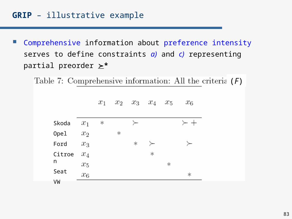
Comprehensive information about preference intensity serves to
define constraints a) and c) representing partial preorder *
(F)
Skoda
Opel
Ford
Citroen
Seat
VW
84
GRIP – illustrative example
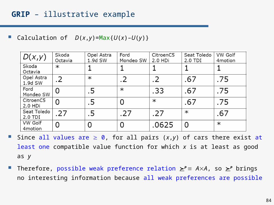
Calculation of D(x,y)=Max{U(x)–U(y)}
Since all values are 0, for all pairs (x,y) of cars there exist at least
one compatible value function for which x is at least as good as y
Therefore, possible weak preference relation P AA, so P brings
no interesting information because all weak preferences are possible
85
GRIP – illustrative example
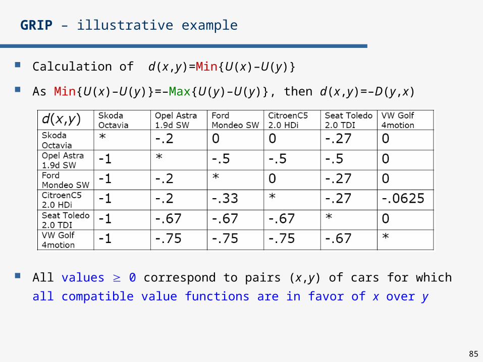
Calculation of d(x,y)=Min{U(x)–U(y)}
As Min{U(x)–U(y)}=–Max{U(y)–U(y)}, then d(x,y)=–D(y,x)
All values 0 correspond to pairs (x,y) of cars for which all compatible
value functions are in favor of x over y
86
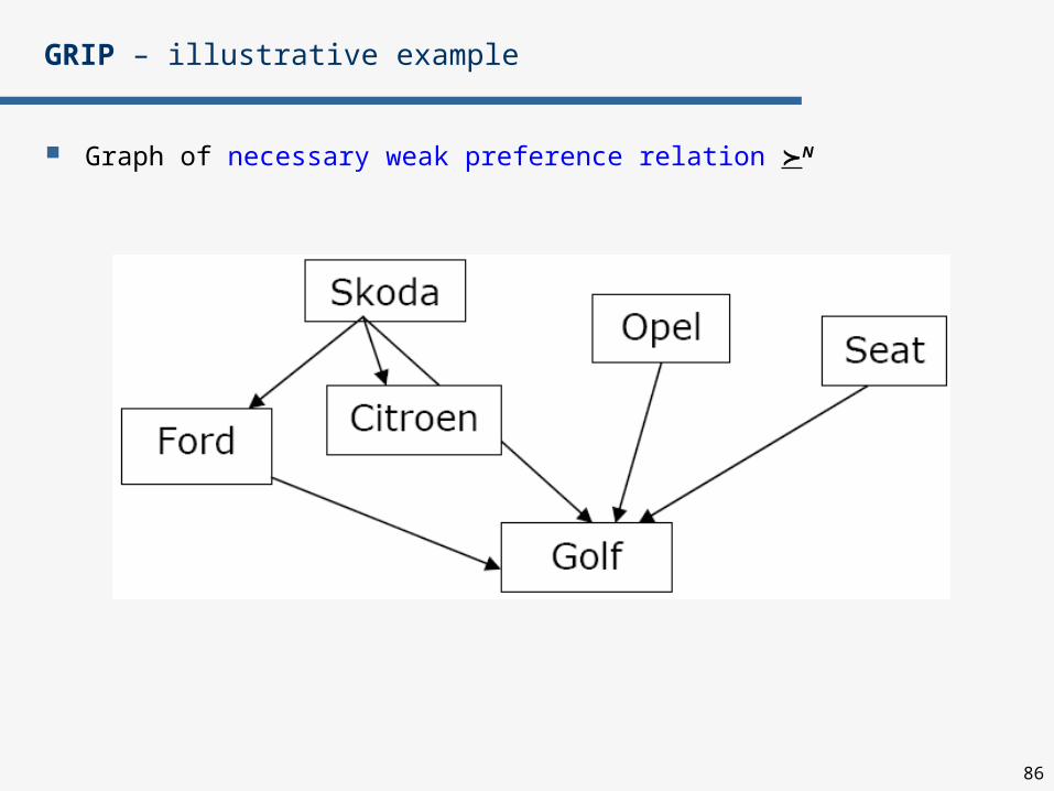
GRIP – illustrative example
Graph of necessary weak preference relation N

87
In GRIP, preference information is given by the DM in terms of:
partial preorder in the set of reference actions
partial and comprehensive comparisons of intensities of preference between some pairs of reference actions,
The preference information is used within regression approach to build a complete set of compatible additive value functions
Considering all compatible value functions permits to find as result:
necessary w.pref. relation in A and in AA (partial preorder) N, *N
possible w.pref. relation in A and in AA (strongly complete) P, *P
Possible extensions:
preference information with gradual credibility
group decision
Conclusions