Role of the Indian Ocean sea surface temperature in shapingthe natural variability in the flow of Nile River

Mohamed S. Siam • Guiling Wang •

Marie-Estelle Demory • Elfatih A. B. Eltahir

Received: 15 April 2013 / Accepted: 31 March 2014

� Springer-Verlag Berlin Heidelberg 2014

Abstract A significant fraction of the inter-annual vari-

ability in the Nile River flow is shaped by El Nino Southern

Oscillation (ENSO). Here, we investigate a similar role for

the Indian Ocean (IO) sea surface temperature (SST) in

shaping the inter-annual variability of the Nile River flow.

Using observations of global SST distribution and river

flow in addition to atmospheric general circulation model

sensitivity experiments, we show that North and Middle IO

SSTs play a significant intermediate role in the telecon-

nection between ENSO and the Nile flow. Applying partial

coherency analyses, we demonstrate that the connection

between North and Middle IO SSTs and Nile flow is

strongly coupled to ENSO. During El Nino events, SST in

the North and Middle IO increases in response to the

warming in the Tropical Eastern Pacific Ocean and forces a

Gill-type circulation with enhanced westerly low-level

flow over East Africa and the Western IO. This anomalous

low-level flow enhances the low-level flux of air and

moisture away from the Upper Blue Nile (UBN) basin

resulting in reduction of rainfall and river flow. SSTs in the

South IO also play a significant role in shaping the vari-

ability of the Nile flow that is independent from ENSO. A

warming over the South IO, generates a cyclonic flow in

the boundary layer, which reduces the cross-equatorial

meridional transport of air and moisture towards the UBN

basin, favoring a reduction in rainfall and river flow. This

independence between the roles of ENSO and South IO

SSTs allows for development of new combined indices of

SSTs to explain the inter-annual variability of the Nile

flow. The proposed teleconnections have important impli-

cations regarding mechanisms that shape the regional

impacts of climate change over the Nile basin.

Keywords Nile � ENSO � Indian Ocean

1 Introduction

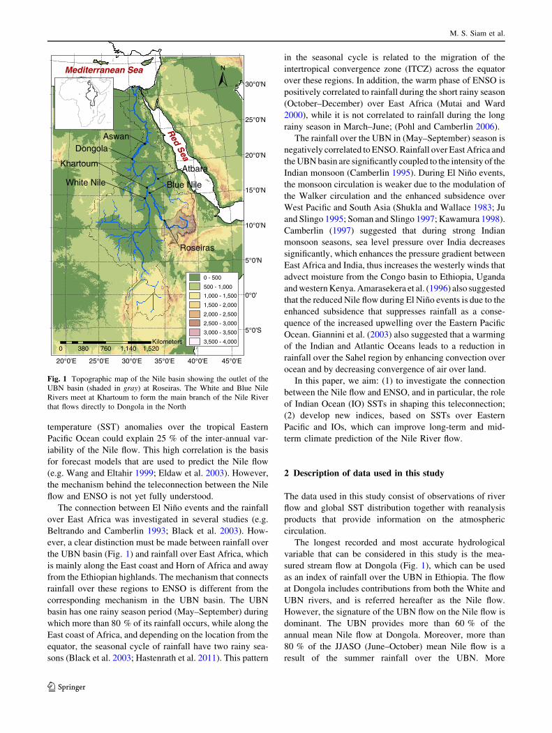
The Nile basin covers an area of 2.9 9 106 km2, which is

approximately 10 % of the African continent (Fig. 1). It

has two main tributaries, the White Nile and the Blue Nile

that originate from the equatorial lakes and Ethiopian

highlands respectively. The Upper Blue Nile (UBN) basin

is the main source of water for the Nile River. It contributes

to approximately 60 % of the main flow of the Nile

(Conway and Hulme 1993). It extends over an area of

175 9 103 km2 (7�N–12�50N, 34�50E–40�E). The mean

annual rainfall over this basin is 1,200 mm/year (Conway

and Hulme 1993). Almost 60 % of the annual rainfall over

the UBN occurs during the summer between July and

August and the river flow lags rainfall by about 1 month

with an average annual volume of 46 km3 based on the

record for the period 1961–1990 (ElShamy 2009).

The inter-annual variability in the flow of the Nile River

is strongly correlated with El Nino Southern Oscillations

(ENSO), its warm phase being associated with a reduced

Nile flow. Eltahir (1996) determined that sea surface

M. S. Siam (&) � E. A. B. Eltahir

Ralph M. Parsons Laboratory, Massachusetts Institute of

Technology, 15 Vassar St., Cambridge, MA 02139, USA

e-mail: msiam@mit.edu

G. Wang

Department of Civil and Environmental Engineering

and Center for Environmental Sciences and Engineering,

University of Connecticut, Storrs, CT, USA

M.-E. Demory

National Centre for Atmospheric Science, Department of

Meteorology, University of Reading, Reading, UK

123

Clim Dyn

DOI 10.1007/s00382-014-2132-6

temperature (SST) anomalies over the tropical Eastern

Pacific Ocean could explain 25 % of the inter-annual var-

iability of the Nile flow. This high correlation is the basis

for forecast models that are used to predict the Nile flow

(e.g. Wang and Eltahir 1999; Eldaw et al. 2003). However,

the mechanism behind the teleconnection between the Nile

flow and ENSO is not yet fully understood.

The connection between El Nino events and the rainfall

over East Africa was investigated in several studies (e.g.

Beltrando and Camberlin 1993; Black et al. 2003). How-

ever, a clear distinction must be made between rainfall over

the UBN basin (Fig. 1) and rainfall over East Africa, which

is mainly along the East coast and Horn of Africa and away

from the Ethiopian highlands. The mechanism that connects

rainfall over these regions to ENSO is different from the

corresponding mechanism in the UBN basin. The UBN

basin has one rainy season period (May–September) during

which more than 80 % of its rainfall occurs, while along the

East coast of Africa, and depending on the location from the

equator, the seasonal cycle of rainfall have two rainy sea-

sons (Black et al. 2003; Hastenrath et al. 2011). This pattern

in the seasonal cycle is related to the migration of the

intertropical convergence zone (ITCZ) across the equator

over these regions. In addition, the warm phase of ENSO is

positively correlated to rainfall during the short rainy season

(October–December) over East Africa (Mutai and Ward

2000), while it is not correlated to rainfall during the long

rainy season in March–June; (Pohl and Camberlin 2006).

The rainfall over the UBN in (May–September) season is

negatively correlated to ENSO. Rainfall over East Africa and

the UBN basin are significantly coupled to the intensity of the

Indian monsoon (Camberlin 1995). During El Nino events,

the monsoon circulation is weaker due to the modulation of

the Walker circulation and the enhanced subsidence over

West Pacific and South Asia (Shukla and Wallace 1983; Ju

and Slingo 1995; Soman and Slingo 1997; Kawamura 1998).

Camberlin (1997) suggested that during strong Indian

monsoon seasons, sea level pressure over India decreases

significantly, which enhances the pressure gradient between

East Africa and India, thus increases the westerly winds that

advect moisture from the Congo basin to Ethiopia, Uganda

and western Kenya. Amarasekera et al. (1996) also suggested

that the reduced Nile flow during El Nino events is due to the

enhanced subsidence that suppresses rainfall as a conse-

quence of the increased upwelling over the Eastern Pacific

Ocean. Giannini et al. (2003) also suggested that a warming

of the Indian and Atlantic Oceans leads to a reduction in

rainfall over the Sahel region by enhancing convection over

ocean and by decreasing convergence of air over land.

In this paper, we aim: (1) to investigate the connection

between the Nile flow and ENSO, and in particular, the role

of Indian Ocean (IO) SSTs in shaping this teleconnection;

(2) develop new indices, based on SSTs over Eastern

Pacific and IOs, which can improve long-term and mid-

term climate prediction of the Nile River flow.

2 Description of data used in this study

The data used in this study consist of observations of river

flow and global SST distribution together with reanalysis

products that provide information on the atmospheric

circulation.

The longest recorded and most accurate hydrological

variable that can be considered in this study is the mea-

sured stream flow at Dongola (Fig. 1), which can be used

as an index of rainfall over the UBN in Ethiopia. The flow

at Dongola includes contributions from both the White and

UBN rivers, and is referred hereafter as the Nile flow.

However, the signature of the UBN flow on the Nile flow is

dominant. The UBN provides more than 60 % of the

annual mean Nile flow at Dongola. Moreover, more than

80 % of the JJASO (June–October) mean Nile flow is a

result of the summer rainfall over the UBN. More

45°0'E40°0'E35°0'E30°0'E25°0'E20°0'E

30°0'N

25°0'N

20°0'N

15°0'N

10°0'N

5°0'N

0°0'

5°0'S

0 380 760 1,140 1,520Kilometers

Mediterranean Sea

Red

Sea

White Nile

0 - 500

500 - 1,000

1,000 - 1,500

1,500 - 2,000

2,000 - 2,500

2,500 - 3,000

3,000 - 3,500

3,500 - 4,000

AswanDongola

Khartoum

Roseiras

Blue Nile

Atbara

Fig. 1 Topographic map of the Nile basin showing the outlet of the

UBN basin (shaded in gray) at Roseiras. The White and Blue Nile

Rivers meet at Khartoum to form the main branch of the Nile River

that flows directly to Dongola in the North

M. S. Siam et al.

123

importantly, the flow in the Blue Nile explains most of the

inter-annual variability in the flow of the Nile River. The

monthly mean flow data at Dongola were extracted from

the Global River Discharge Database (RivDIS v 1.1) for

the period 1871–2000 (Vorosmarty et al. 1998).

The SST data were extracted from the global monthly

mean (HadISST V 1.1) dataset, available on a 1 � latitude–

longitude grid from 1871 to 2000 (Rayner et al. 2003).

Monthly anomalies of the SSTs were averaged over three

Eastern Pacific Ocean regions (2�N–6�N, 170�W–90�W;

6�S–2�N, 180�W–90�W; 10�S–6�S, 150�W–110�W) and

used as ENSO indices. These regions have the highest cor-

relations with the mean Nile flow and cover the same areas as

the Nino 3 and 3.4 indices (Trenberth 1997). In addition,

monthly anomalies of SSTs were averaged over three dif-

ferent regions in the IO. These regions are defined hereafter

as the North IO (0–15�N, 50�E–70�E), the Middle IO (10�S–

0, 50�E–70�E) and the South IO (25�S–35�S, 50�E–80�E).

Also, these regions exhibit the highest correlations with the

Nile flow, compared to other regions of the IO.

The variables considered to study the atmospheric circu-

lation in response to changes in SST include zonal and

meridional wind speed components on pressure levels. These

are obtained from the ERA-Interim (ERAI) reanalysis product

for the period 1979–2010 (Dee et al. 2011). ERAI was chosen

among other reanalysis products because it has the most

accurate representation of the hydrological cycle over the

UBN basin (Siam et al. 2013) and wind circulation over Africa

compared to other reanalysis products such as ERA40

(Uppala et al. 2005) or NCEP–NCAR (Kalnay et al. 1996).

3 Observational analyses of the relationships

between Nile flow and SSTs in Indian and Pacific

Oceans

3.1 Cross-correlation analyses

In this section, a detailed analysis of correlations between

SSTs over the Indian and Pacific Oceans and the Nile flow

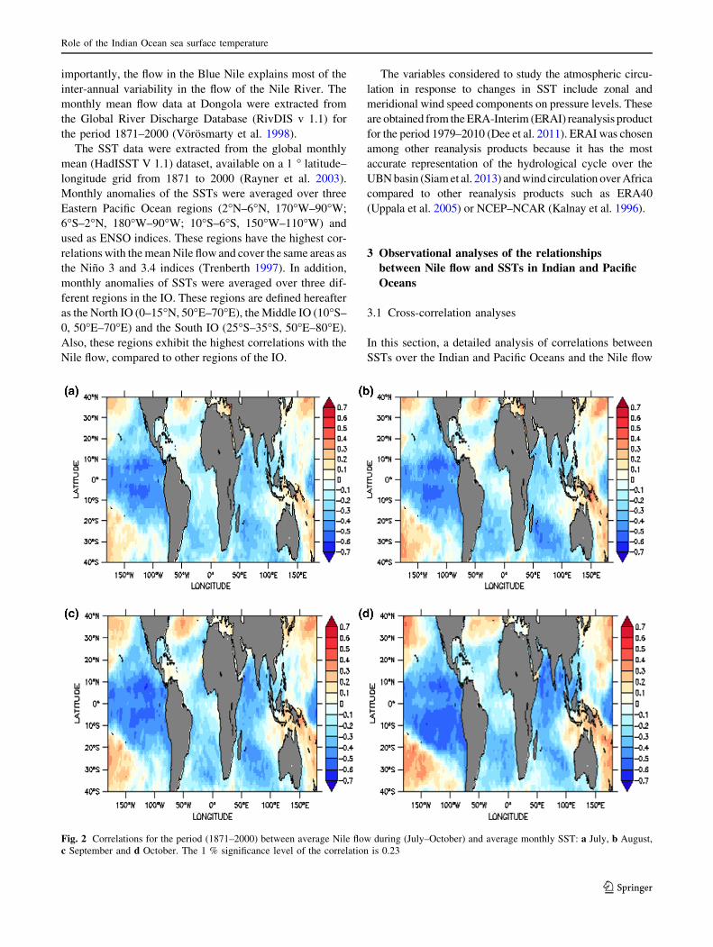
Fig. 2 Correlations for the period (1871–2000) between average Nile flow during (July–October) and average monthly SST: a July, b August,

c September and d October. The 1 % significance level of the correlation is 0.23

Role of the Indian Ocean sea surface temperature

123

is presented. From July to October, tropical Eastern Pacific

SSTs show a persistent and significant negative correlation

with the JASO (July–October) mean Nile flow for the

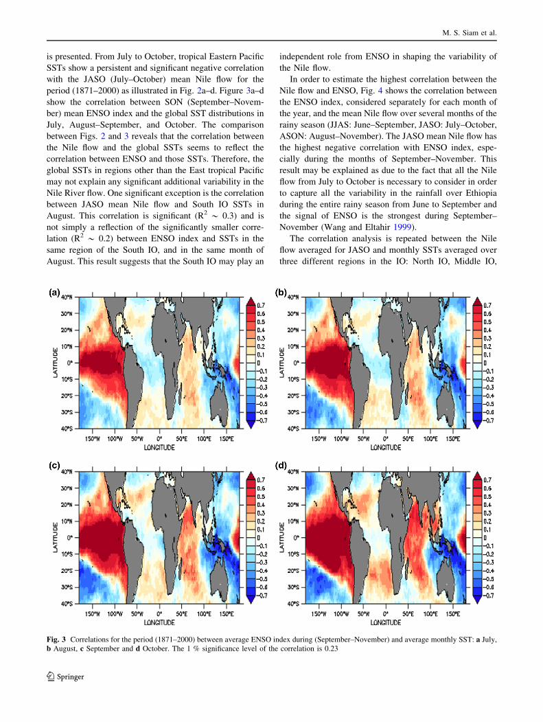
period (1871–2000) as illustrated in Fig. 2a–d. Figure 3a–d

show the correlation between SON (September–Novem-

ber) mean ENSO index and the global SST distributions in

July, August–September, and October. The comparison

between Figs. 2 and 3 reveals that the correlation between

the Nile flow and the global SSTs seems to reflect the

correlation between ENSO and those SSTs. Therefore, the

global SSTs in regions other than the East tropical Pacific

may not explain any significant additional variability in the

Nile River flow. One significant exception is the correlation

between JASO mean Nile flow and South IO SSTs in

August. This correlation is significant (R2 * 0.3) and is

not simply a reflection of the significantly smaller corre-

lation (R2 * 0.2) between ENSO index and SSTs in the

same region of the South IO, and in the same month of

August. This result suggests that the South IO may play an

independent role from ENSO in shaping the variability of

the Nile flow.

In order to estimate the highest correlation between the

Nile flow and ENSO, Fig. 4 shows the correlation between

the ENSO index, considered separately for each month of

the year, and the mean Nile flow over several months of the

rainy season (JJAS: June–September, JASO: July–October,

ASON: August–November). The JASO mean Nile flow has

the highest negative correlation with ENSO index, espe-

cially during the months of September–November. This

result may be explained as due to the fact that all the Nile

flow from July to October is necessary to consider in order

to capture all the variability in the rainfall over Ethiopia

during the entire rainy season from June to September and

the signal of ENSO is the strongest during September–

November (Wang and Eltahir 1999).

The correlation analysis is repeated between the Nile

flow averaged for JASO and monthly SSTs averaged over

three different regions in the IO: North IO, Middle IO,

Fig. 3 Correlations for the period (1871–2000) between average ENSO index during (September–November) and average monthly SST: a July,

b August, c September and d October. The 1 % significance level of the correlation is 0.23

M. S. Siam et al.

123

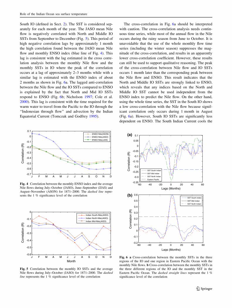
South IO (defined in Sect. 2). The SST is considered sep-

arately for each month of the year. The JASO mean Nile

flow is negatively correlated with North and Middle IO

SSTs from September to December (Fig. 5). This period of

high negative correlation lags by approximately 1 month

the high correlation found between the JASO mean Nile

flow and monthly ENSO index (blue line of Fig. 4). This

lag is consistent with the lag estimated in the cross corre-

lation analysis between the monthly Nile flow and the

monthly SSTs in IO where the peak of the correlation

occurs at a lag of approximately 2–3 months while with a

similar lag is estimated with the ENSO index of about

2 months as shown in Fig. 6a. The lagged anti-correlation

between the Nile flow and the IO SSTs compared to ENSO

is explained by the fact that North and Mid IO SSTs

respond to ENSO (Fig. 6b; Nicholson 1997; Cole et al.

2000). This lag is consistent with the time required for the

warm water to travel from the Pacific to the IO through the

‘‘Indonesian through flow’’ and advection by the Indian

Equatorial Current (Tomczak and Godfrey 1995).

The cross-correlation in Fig. 6a should be interpreted

with caution. The cross-correlation analysis needs contin-

uous time series, while most of the annual flow in the Nile

occurs during the rainy season from June to October. It is

unavoidable that the use of the whole monthly flow time

series (including the winter season) suppresses the mag-

nitude of the cross-correlation, and results in an apparently

lower cross-correlation coefficient. However, these results

can still be used to support qualitative reasoning. The peak

of the cross-correlation between Nile flow and IO SSTs

occurs 1 month later than the corresponding peak between

the Nile flow and ENSO. This result indicates that the

North and Middle IO SSTs are strongly linked to ENSO,

which reveals that any indices based on the North and

Middle IO SST cannot be used independent from the

ENSO index to predict the Nile flow. On the other hand,

using the whole time series, the SST in the South IO shows

a low cross-correlation with the Nile flow because signif-

icant correlation only occurs during 1 month in August

(Fig. 6a). However, South IO SSTs are significantly less

dependent on ENSO. The South Indian Current cools the

J F M A M J J A S O N D-0.7

-0.6

-0.5

-0.4

-0.3

-0.2

-0.1

0

0.1

Cor

rela

tion

(R)

ENSO-Nile(ASON)

ENSO-Nile(JASO)

ENSO-Nile(JJAS)

Fig. 4 Correlation between the monthly ENSO index and the average

Nile flows during July–October (JASO), June–September (JJAS) and

August–November (ASON) for 1871–2000. The dashed line repre-

sents the 1 % significance level of the correlation

J F M A M J J A S O N D-0.6

-0.5

-0.4

-0.3

-0.2

-0.1

0

Month

Cor

rela

tion

(R)

Indian South-Nile(JASO)

Indian North-Nile(JASO)

Indian Mid-Nile(JASO)

Fig. 5 Correlation between the monthly IO SSTs and the average

Nile flows during July–October (JASO) for 1871–2000. The dashed

line represents the 1 % significance level of the correlation

-60 -40 -20 0 20 40 60-0.2

-0.1

0

0.1

0.2

0.3

0.4

0.5

0.6

Lags (Months)

Cor

rela

tion

(R)

SST South Indian

SST Mid Indian

SST North Indian

-60 -40 -20 0 20 40 60-0.35

-0.3

-0.25

-0.2

-0.15

-0.1

-0.05

0

0.05

0.1

Lags (Months)

Cor

rela

tion

(R)

SST South Indian

SST Mid Indian

SST North Indian

Eastern Pacific

(a)

(b)

Fig. 6 a Cross-correlation between the monthly SSTs in the three

regions of the IO and one region in Eastern Pacific Ocean with the

monthly Nile flows. b Cross-correlation between the monthly SSTs in

the three different regions of the IO and the monthly SST in the

Eastern Pacific Ocean. The dashed straight lines represent the 1 %

significance level of the correlation

Role of the Indian Ocean sea surface temperature

123

South IO surface and decreases the effect of the warm

South Equatorial Current on the South IO (Tomczak and

Godfrey 1995).

3.2 Partial coherency analysis

The dependence of the Nile flow on SSTs in the Indian and

Pacific Oceans is analyzed in this section using partial

coherency analysis. ‘‘Partial coherency’’ represents a gen-

eralization of the concept of partial correlation coefficient.

Partial correlation analysis focuses on the relationship

between two variables in the presence of a third variable

(Jobson 1991). It quantifies the correlation between these

two variables after evaluating the impact of the third var-

iable. In this study, the two variables are the Nile flow and

IO SSTs, and the third variable is the ENSO index. The

partial correlation coefficient quantifies how much of the

Nile flow variability, which cannot be explained by ENSO,

is explained by IO SSTs. However, the partial correlation

coefficient does not show how this correlation is distributed

over different frequencies. Here, we apply the partial

coherency analysis, which describes how the partial cor-

relation is distributed among different frequencies. By

‘‘partial coherency’’, we mean the cross-coherency

between IO SSTs and the portion of the Nile flow vari-

ability that cannot be explained by ENSO.

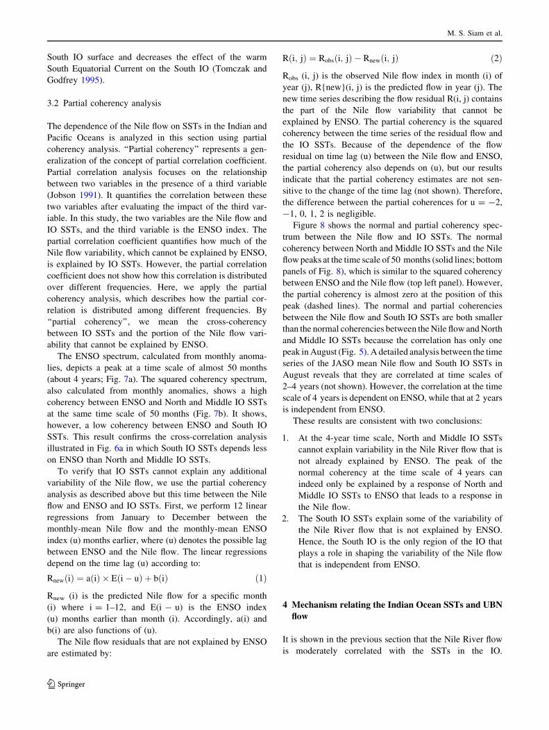
The ENSO spectrum, calculated from monthly anoma-

lies, depicts a peak at a time scale of almost 50 months

(about 4 years; Fig. 7a). The squared coherency spectrum,

also calculated from monthly anomalies, shows a high

coherency between ENSO and North and Middle IO SSTs

at the same time scale of 50 months (Fig. 7b). It shows,

however, a low coherency between ENSO and South IO

SSTs. This result confirms the cross-correlation analysis

illustrated in Fig. 6a in which South IO SSTs depends less

on ENSO than North and Middle IO SSTs.

To verify that IO SSTs cannot explain any additional

variability of the Nile flow, we use the partial coherency

analysis as described above but this time between the Nile

flow and ENSO and IO SSTs. First, we perform 12 linear

regressions from January to December between the

monthly-mean Nile flow and the monthly-mean ENSO

index (u) months earlier, where (u) denotes the possible lag

between ENSO and the Nile flow. The linear regressions

depend on the time lag (u) according to:

RnewðiÞ ¼ aðiÞ � Eði� uÞ þ bðiÞ ð1Þ

Rnew (i) is the predicted Nile flow for a specific month

(i) where i = 1–12, and E(i - u) is the ENSO index

(u) months earlier than month (i). Accordingly, a(i) and

b(i) are also functions of (u).

The Nile flow residuals that are not explained by ENSO

are estimated by:

R i; jð Þ ¼ Robs i; jð Þ � Rnew i; jð Þ ð2Þ

Robs (i, j) is the observed Nile flow index in month (i) of

year (j), R{new}(i, j) is the predicted flow in year (j). The

new time series describing the flow residual R(i, j) contains

the part of the Nile flow variability that cannot be

explained by ENSO. The partial coherency is the squared

coherency between the time series of the residual flow and

the IO SSTs. Because of the dependence of the flow

residual on time lag (u) between the Nile flow and ENSO,

the partial coherency also depends on (u), but our results

indicate that the partial coherency estimates are not sen-

sitive to the change of the time lag (not shown). Therefore,

the difference between the partial coherences for u = -2,

-1, 0, 1, 2 is negligible.

Figure 8 shows the normal and partial coherency spec-

trum between the Nile flow and IO SSTs. The normal

coherency between North and Middle IO SSTs and the Nile

flow peaks at the time scale of 50 months (solid lines; bottom

panels of Fig. 8), which is similar to the squared coherency

between ENSO and the Nile flow (top left panel). However,

the partial coherency is almost zero at the position of this

peak (dashed lines). The normal and partial coherencies

between the Nile flow and South IO SSTs are both smaller

than the normal coherencies between the Nile flow and North

and Middle IO SSTs because the correlation has only one

peak in August (Fig. 5). A detailed analysis between the time

series of the JASO mean Nile flow and South IO SSTs in

August reveals that they are correlated at time scales of

2–4 years (not shown). However, the correlation at the time

scale of 4 years is dependent on ENSO, while that at 2 years

is independent from ENSO.

These results are consistent with two conclusions:

1. At the 4-year time scale, North and Middle IO SSTs

cannot explain variability in the Nile River flow that is

not already explained by ENSO. The peak of the

normal coherency at the time scale of 4 years can

indeed only be explained by a response of North and

Middle IO SSTs to ENSO that leads to a response in

the Nile flow.

2. The South IO SSTs explain some of the variability of

the Nile River flow that is not explained by ENSO.

Hence, the South IO is the only region of the IO that

plays a role in shaping the variability of the Nile flow

that is independent from ENSO.

4 Mechanism relating the Indian Ocean SSTs and UBN

flow

It is shown in the previous section that the Nile River flow

is moderately correlated with the SSTs in the IO.

M. S. Siam et al.

123

100

101

102

0

0.5

1

1.5

2

Months

Spe

ctru

m

Sprectrum of ENSO

100

101

102

0

0.2

0.4

0.6

0.8

1

Months

Squ

ared

Coh

eren

cy (

R2)

Squared Coherency between ENSO index and Indian Ocean SSTs

South Indian

Mid Indian

North Indian

(a)

(b)

Fig. 7 a Spectrum of ENSO,

b squared coherency between

ENSO and SSTS in the IO. The

straight dashed line represents

the 1 % significance level of the

correlation

100

101

102

0

0.2

0.4

0.6

Months

Squ

ared

Coh

eren

cy (

R2 )

Squared Coherency between Nile flow and ENSO

100

101

102

0

0.2

0.4

0.6

Months

Squ

ared

Coh

eren

cy (

R2 )

Squared Coherency between Nile flow and South Indian SST

100

101

102

0

0.2

0.4

0.6

Months

Squ

ared

Coh

eren

cy (

R2 )

Squared Coherency between Nile flow and Middle Indian SST

100

101

102

0

0.2

0.4

0.6

Months

Squ

ared

Coh

eren

cy (

R2 )

Squared Coherency between Nile flow and North Indian SST

Normal Coherency

Partial Coherency

Normal Coherency

Partial CoherencyNormal Coherency

Partial Coherency

Fig. 8 Squared Coherency

between the Nile flows and

SSTs in the Pacific (ENSO

index) and IO. The straight

dashed lines represent the 1 %

significance level of the

correlation

Role of the Indian Ocean sea surface temperature

123

Furthermore, we found that the SSTs in the North and

Middle IO respond to the warming in the Pacific, while the

SSTs of South IO are less dependent on the Pacific SSTs.

In this section we propose a mechanism that explains these

teleconnections between ENSO, IO SSTs and Nile flow.

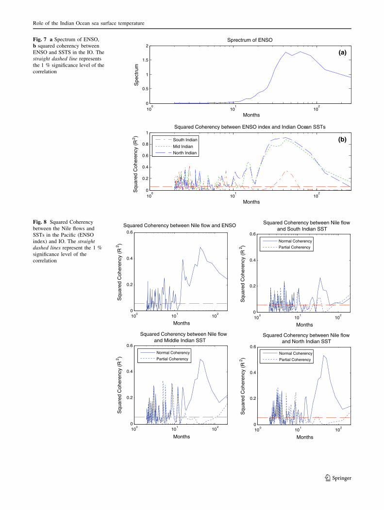
Figure 9 shows the ERAI averaged wind fluxes at 800

mb during August 1979–2011. The wind circulation is

mainly composed of two anticyclones in the North and

South of the Equator. The anticyclone located in the South

is responsible for maintaining the cross-equatorial meridi-

onal southerly flow and the associated convergence of air

over the UBN basin. The anticyclone located in the North

is associated with low level westerly winds that forces

divergence of air away from the UBN.

The intensity of the anticyclonic circulations is reflected in

the magnitude of the relative vorticity: strong westerly and

cross-equatorial southerly low-level flows correspond to high

values of relative vorticity over the North and South IO,

respectively. It is important to notice that the sign of vorticity

in the South of IO is positive (anti-clockwise) and negative

(clockwise) in the North of IO (Fig. 9). The correlation

between relative vorticity at 700 mb and convergence of air in

the lowest 300 mb over the UBN basin in July is shown on

Fig. 10a, and that for August is shown on Fig. 11a. The

Fig. 9 Average wind

circulation during August

(1979–2011) at 800 mb using

ERAI reanalysis product. The

UBN basin (shaded in brown)

(a) (b)

Fig. 10 a Correlation between the relative vorticity at 700 mb over

the IO and averaged convergence of air in the lowest 300 mb over the

UBN basin (shaded in brown) during July, and b correlation between

average relative vorticity over (60�E–80�E and 5�S–10�N) and SSTs

in the IO during July

M. S. Siam et al.

123

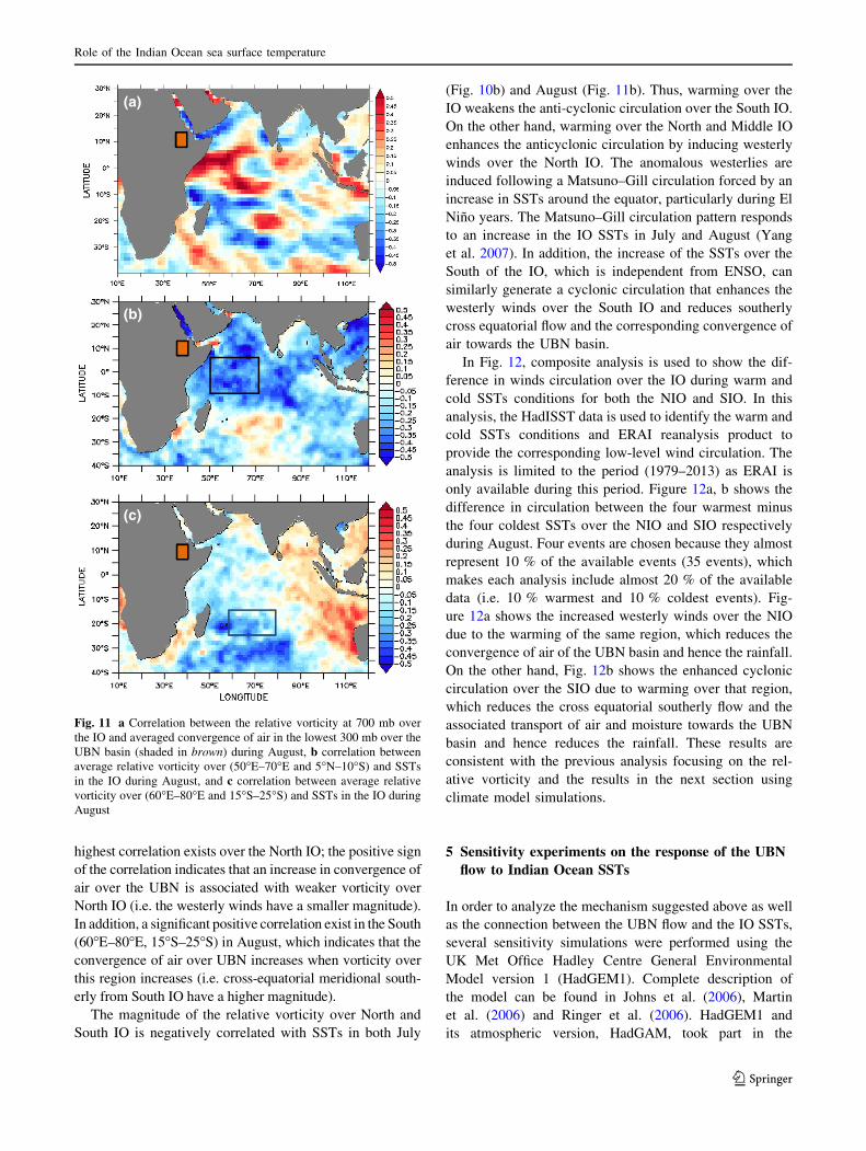
highest correlation exists over the North IO; the positive sign

of the correlation indicates that an increase in convergence of

air over the UBN is associated with weaker vorticity over

North IO (i.e. the westerly winds have a smaller magnitude).

In addition, a significant positive correlation exist in the South

(60�E–80�E, 15�S–25�S) in August, which indicates that the

convergence of air over UBN increases when vorticity over

this region increases (i.e. cross-equatorial meridional south-

erly from South IO have a higher magnitude).

The magnitude of the relative vorticity over North and

South IO is negatively correlated with SSTs in both July

(Fig. 10b) and August (Fig. 11b). Thus, warming over the

IO weakens the anti-cyclonic circulation over the South IO.

On the other hand, warming over the North and Middle IO

enhances the anticyclonic circulation by inducing westerly

winds over the North IO. The anomalous westerlies are

induced following a Matsuno–Gill circulation forced by an

increase in SSTs around the equator, particularly during El

Nino years. The Matsuno–Gill circulation pattern responds

to an increase in the IO SSTs in July and August (Yang

et al. 2007). In addition, the increase of the SSTs over the

South of the IO, which is independent from ENSO, can

similarly generate a cyclonic circulation that enhances the

westerly winds over the South IO and reduces southerly

cross equatorial flow and the corresponding convergence of

air towards the UBN basin.

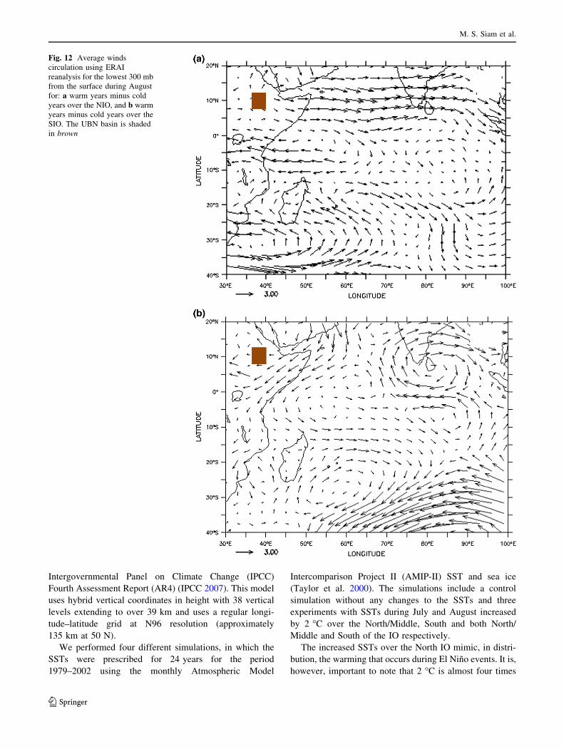
In Fig. 12, composite analysis is used to show the dif-

ference in winds circulation over the IO during warm and

cold SSTs conditions for both the NIO and SIO. In this

analysis, the HadISST data is used to identify the warm and

cold SSTs conditions and ERAI reanalysis product to

provide the corresponding low-level wind circulation. The

analysis is limited to the period (1979–2013) as ERAI is

only available during this period. Figure 12a, b shows the

difference in circulation between the four warmest minus

the four coldest SSTs over the NIO and SIO respectively

during August. Four events are chosen because they almost

represent 10 % of the available events (35 events), which

makes each analysis include almost 20 % of the available

data (i.e. 10 % warmest and 10 % coldest events). Fig-

ure 12a shows the increased westerly winds over the NIO

due to the warming of the same region, which reduces the

convergence of air of the UBN basin and hence the rainfall.

On the other hand, Fig. 12b shows the enhanced cyclonic

circulation over the SIO due to warming over that region,

which reduces the cross equatorial southerly flow and the

associated transport of air and moisture towards the UBN

basin and hence reduces the rainfall. These results are

consistent with the previous analysis focusing on the rel-

ative vorticity and the results in the next section using

climate model simulations.

5 Sensitivity experiments on the response of the UBN

flow to Indian Ocean SSTs

In order to analyze the mechanism suggested above as well

as the connection between the UBN flow and the IO SSTs,

several sensitivity simulations were performed using the

UK Met Office Hadley Centre General Environmental

Model version 1 (HadGEM1). Complete description of

the model can be found in Johns et al. (2006), Martin

et al. (2006) and Ringer et al. (2006). HadGEM1 and

its atmospheric version, HadGAM, took part in the

(a)

(b)

(c)

Fig. 11 a Correlation between the relative vorticity at 700 mb over

the IO and averaged convergence of air in the lowest 300 mb over the

UBN basin (shaded in brown) during August, b correlation between

average relative vorticity over (50�E–70�E and 5�N–10�S) and SSTs

in the IO during August, and c correlation between average relative

vorticity over (60�E–80�E and 15�S–25�S) and SSTs in the IO during

August

Role of the Indian Ocean sea surface temperature

123

Intergovernmental Panel on Climate Change (IPCC)

Fourth Assessment Report (AR4) (IPCC 2007). This model

uses hybrid vertical coordinates in height with 38 vertical

levels extending to over 39 km and uses a regular longi-

tude–latitude grid at N96 resolution (approximately

135 km at 50 N).

We performed four different simulations, in which the

SSTs were prescribed for 24 years for the period

1979–2002 using the monthly Atmospheric Model

Intercomparison Project II (AMIP-II) SST and sea ice

(Taylor et al. 2000). The simulations include a control

simulation without any changes to the SSTs and three

experiments with SSTs during July and August increased

by 2 �C over the North/Middle, South and both North/

Middle and South of the IO respectively.

The increased SSTs over the North IO mimic, in distri-

bution, the warming that occurs during El Nino events. It is,

however, important to note that 2 �C is almost four times

Fig. 12 Average winds

circulation using ERAI

reanalysis for the lowest 300 mb

from the surface during August

for: a warm years minus cold

years over the NIO, and b warm

years minus cold years over the

SIO. The UBN basin is shaded

in brown

M. S. Siam et al.

123

the standard deviation of the SST variation in these regions.

The intention for applying such a large SST warming is to

force the model to respond strongly, which makes it easier

to analyze the results than with a weak warming. Further-

more, as shown in the previous sections, the SSTs are

increased over the South IO to show their independent

impact from ENSO on the Nile River flow. The monthly

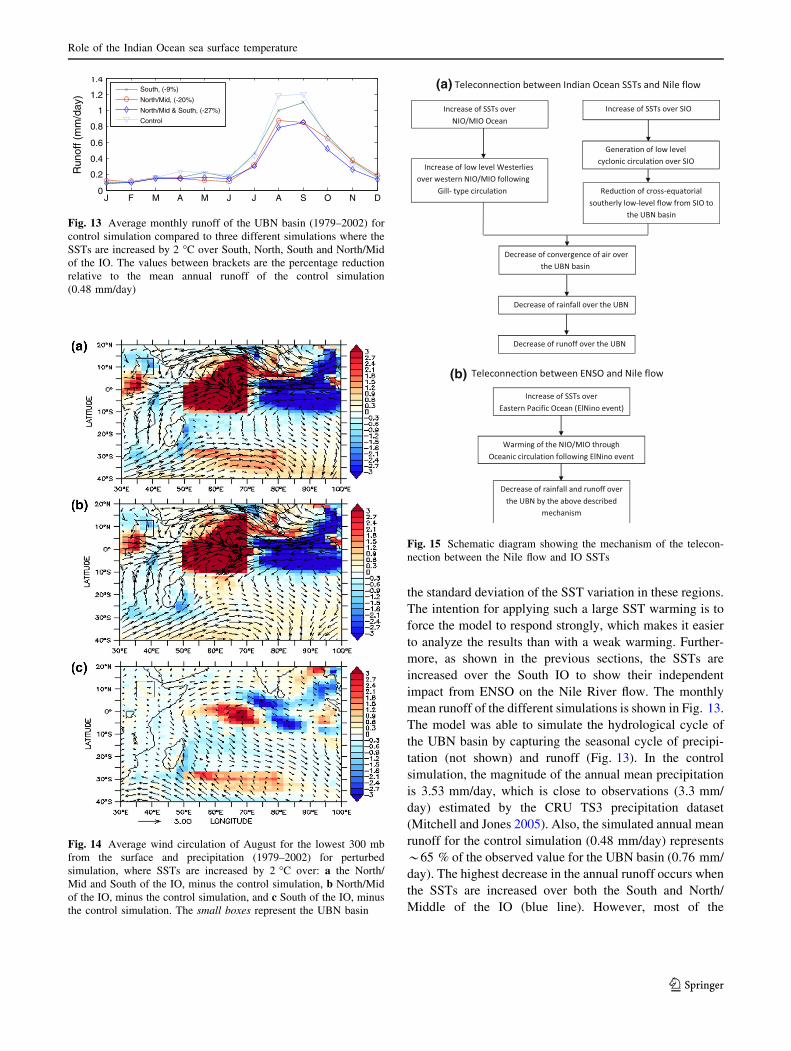
mean runoff of the different simulations is shown in Fig. 13.

The model was able to simulate the hydrological cycle of

the UBN basin by capturing the seasonal cycle of precipi-

tation (not shown) and runoff (Fig. 13). In the control

simulation, the magnitude of the annual mean precipitation

is 3.53 mm/day, which is close to observations (3.3 mm/

day) estimated by the CRU TS3 precipitation dataset

(Mitchell and Jones 2005). Also, the simulated annual mean

runoff for the control simulation (0.48 mm/day) represents

*65 % of the observed value for the UBN basin (0.76 mm/

day). The highest decrease in the annual runoff occurs when

the SSTs are increased over both the South and North/

Middle of the IO (blue line). However, most of the

J F M A M J J A S O N D0

0.2

0.4

0.6

0.8

1

1.2

1.4R

unof

f (m

m/d

ay)

South, (-9%)

North/Mid, (-20%)

North/Mid & South, (-27%)

Control

Fig. 13 Average monthly runoff of the UBN basin (1979–2002) for

control simulation compared to three different simulations where the

SSTs are increased by 2 �C over South, North, South and North/Mid

of the IO. The values between brackets are the percentage reduction

relative to the mean annual runoff of the control simulation

(0.48 mm/day)

Fig. 14 Average wind circulation of August for the lowest 300 mb

from the surface and precipitation (1979–2002) for perturbed

simulation, where SSTs are increased by 2 �C over: a the North/

Mid and South of the IO, minus the control simulation, b North/Mid

of the IO, minus the control simulation, and c South of the IO, minus

the control simulation. The small boxes represent the UBN basin

(a)

(b)

Fig. 15 Schematic diagram showing the mechanism of the telecon-

nection between the Nile flow and IO SSTs

Role of the Indian Ocean sea surface temperature

123

reduction is related to the increased SSTs over the North/

Middle of IO (red line). The highest decrease of the runoff is

relatively large (i.e. 27 %), relative the coefficient of vari-

ation in the observed flow *22 %, which indicates that the

UBN flow is sensitive to the warming over selected regions

and that SSTs are negatively correlated with the UBN flow.

In addition, it is important to notice that we made these

experiments with one model; it is possible that other models

may have stronger response on the Nile flow for the

warming of the IO.

The corresponding anomalous wind circulations for the

simulation in which the SSTs are increased over the North/

Mid and South IO are shown in Fig. 14. The anomalous

westerlies are seen for August along the coast of Africa and

over the North/Middle IO following the Matsuno–Gill

circulations. These anomalous circulations reduce conver-

gence of air in the boundary layer over the UBN basin and

thus the precipitation and the runoff over the basin. The

response of the circulation to the warming in the South IO

is relatively weak, and fails to reduce the expected impact

on the cross-equatorial southerly low-level flow towards

the UBN basin. As a result the magnitude of the impact on

rainfall and runoff seems low. The mechanism of the

teleconnection between the Nile flow and the ENSO and IO

SSTs is summarized in Fig. 15.

6 Conclusions

In this paper, we investigate the connections between the

Nile flow, IO SSTs and ENSO. We show that SSTs over

North and Middle IO are responding to the warming of the

Pacific Ocean, particularly during El Nino events. More-

over, they do not force any independent significant vari-

ability of the Nile River flow. However, the SSTs over the

South of IO are less dependent on ENSO and explain some

of the variability of the Nile flow that is not explained by

ENSO.

A mechanism that connects the Nile flow to SSTs in IO

and the Pacific Ocean is investigated in this study. The

increase of the SSTs over the North and Middle of the IO,

during El Nino events, forces a Matsuno–Gill circulation

over these regions, which enhances westerly winds and

reduces the convergence of air over the UBN basin. Sim-

ilarly the increase in SSTs over the South IO generates an

anomalous cyclonic circulation that reduces the cross-

equatorial southerly low-level flow and the associated

convergence of air towards the UBN basin. This reduction

in convergence of air is translated to a reduction of rainfall

and runoff over the UBN basin. This mechanism was

simulated using an atmospheric general circulation model

(AGCM) forced with observed SSTs that were modified to

simulate a warming over the IO. It is shown that increasing

SSTs over IO reduces the Nile flow, which highlights some

of the potential mechanisms shaping the impact of climate

change on the Nile River flow, through warming of the

Pacific and IOs.

References

Amarasekera KN, Lee RF, Williams ER, Eltahir EA (1996) B: ENSO

and the natural variability in the flow of tropical rivers. J Hydrol

200:24–39

Beltrando G, Camberlin P (1993) Interannual variability of rainfall in

Eastern Horn of Africa and indicators of atmospheric circulation.

Int J Climatol 13:533–546

Black E, Slingo J, Sperber KR (2003) An observational study of the

relationship between excessively strong short rains in coastal

East Africa and Indian Ocean SST. Mon Weather Rev 31:74–94

Camberlin P (1995) June–September rainfall in North-Eastern Africa

and atmospheric signals over the tropics: a zonal perspective. Int

J Climatol 15:773–783

Camberlin Pierre (1997) Rainfall anomalies in the source region of

the Nile and their connection with the Indian summer monsoon.

J Clim 10:1380–1392

Cole JE et al (2000) Tropical pacific forcing of decadal SST

variability in the western Indian Ocean over the past two

centuries. Science 287(5453):617–619

Conway D, Hulme M (1993) Recent fluctuations in precipitation and

runoff over the Nile sub-basins and their impact on main Nile

discharge. Clim Change 25:127–151

Dee DP et al (2011) The ERA-Interim reanalysis: configuration and

performance of the data assimilation system. Q J R Meteorol Soc

137:553–597

ElDaw A, Salas JD, Garcia LA (2003) Long-range forecasting of the

Nile River flows using climate forcing. J Appl Meteorol 42:

890–904

ElShamy ME (2009) Impacts of climate change on Blue Nile flows

using bias corrected GCM scenarios. Hydrol Earth Syst Sci

13:551–565

Eltahir EAB (1996) ElNino and the natural variability in the flow of

the Nile River. Water Resour Res 32(1):131–137

Giannini A, Saravanan R, Chang P (2003) Oceanic forcing of Sahel

rainfall on interannual to interdecadal time scales. Science

302:1027–1030

Hastenrath Stefan, Polzin Dierk, Mutai Charles (2011) Circulation

mechanisms of Kenya rainfall anomalies. J Clim 24:404–412

IPCC (2007) The physical science basis. Contribution of working

group I to the fourth assessment report of the intergovernmental

panel on climate change. In: Solomon S, Qin D, Manning M,

Chen Z, Marquis M, Averyt KB, Tignor M, Miller HL (eds)

Climate change 2007. Cambridge University Press, Cambridge,

United Kingdom and New York, NY, USA

Jobson JD (1991) Applied multivariate data analysis. Volume I:

regression and experimental design. Springer, New York,

pp 182–185

Johns TC et al (2006) The new hadley centre climate model

(HadGEM1): evaluation of coupled simulations. J Clim 19:

1327–1353

Ju J, Slingo JM (1995) The Asian summer monsoon and ENSO. Q J R

Meteorol Soc 121:1133–1168

Kalnay E et al (1996) The NCEP/NCAR 40-year reanalysis project.

Bull Am Meteorol Soc 77:437–471

Kawamura R (1998) A possible mechanism of the Asian summer

monsoon-ENSO coupling. J Meteorol Soc Jpn 76:1009–1027

M. S. Siam et al.

123

Martin GM, Ringer MA, Pope VD, Jones A, Dearden C, Hinton TJ

(2006) The physical properties of the atmosphere in the New

Hadley Centre Global Environmental Model (HadGEM1). Part I:

model description and global climatology. J Clim 19(7):1274–

1301. doi:10.1175/JCLI3636.1

Mitchell TD, Jones PD (2005) An improved method of constructing a

database of monthly climate observations and associated high-

resolution grids. Int J Climatol 25:693–712

Mutai Charles C, Neil Ward M (2000) East African rainfall and the

tropical circulation/convection on intraseasonal to interannual

timescales. J Clim 13:3915–3939

Nicholson Sharon E (1997) An analysis of the ENSO signal in the

tropical Atlantic and western Indian Oceans. Int J Climatol

17(4):345–375

Pohl B, Camberlin P (2006) Influence of the Madden–Julian oscillation

on East African rainfall. Part I: intraseasonal variability and

regional dependency. Q J R Meteorol Soc 132:2521–2539

Rayner NA, Parker DE, Horton EB, Folland CK, Alexander LV,

Rowell DP, Kent EC, Kaplan A (2003) Global analyses of sea

surface temperature, sea ice, and night marine air temperature

since the late nineteenth century. J Geophys Res 108(D14):4407

Ringer MA, Martin GM, Greeves CZ, Hinton TJ, James PM, Pope

VD, Scaife AA, Stratton RA, Inness PM, Slingo JM, Yang GY

(2006) The physical properties of the atmosphere in the New

Hadley Centre Global Environmental Model (HadGEM1). Part

II: aspects of variability and regional. J Clim 19:1302–1326

Shukla J, Wallace JM (1983) Numerical simulation of the atmo-

spheric response to equatorial Pacific sea surface temperature

anomalies. J Atmos Sci 40:1613–1630

Siam SM, Demory ME, Eltahir EAB Hydrological cycles over the

Congo and upper Blue Nile basins: evaluation of general

circulation models simulations and reanalysis data products.

J Clim. doi:10.1175/JCLI-D-12-00404.1

Soman MK, Slingo J (1997) Sensitivity of the Asian summer

monsoon to aspects of sea-surface-temperature anomalies in the

tropical Pacific Ocean. Q J R Meteorol Soc 123:309–336

Taylor KE, Williamson D, Zwiers F (2000) The sea surface

temperature and sea-ice concentration boundary conditions for

AMIP II simulations. Technical Report 60, PCMDI

Tomczak M, Godfrey JS (1995) Regional oceanography: an intro-

duction. Pregamon, London

Trenberth KE (1997) The definition of El Nino. Bull Am Meteorol

Soc 78:2771–2777

Uppala SM et al (2005) The ERA-40 re-analysis. Q J R Meteorol Soc

131:2961–3012

Vorosmarty CJ, Fekete B, Tucker BA (1998) River discharge

database, Version 1.1 (RivDIS v 1.0 supplement). Available

through the institute for the study of earth, oceans and space

University of New Hampshire, Durham NH (USA)

Wang G, Eltahir EAB (1999) Use of ENSO information in medium

and long range forecasting of the Nile floods. J Clim 12:

1726–1737

Yang JL, Liu QY, Xie SP et al (2007) Impact of the Indian Ocean

SST basin mode on the Asian summer monsoon. Geophys Res

Lett 34:L02708. doi:10.1029/2006GL028571

Role of the Indian Ocean sea surface temperature

123