Embed Size (px)
Citation preview

1
Diagnosis of decadal predictability of Southern Ocean sea surface temperature in 1
the GFDL CM2.1 model 2
Liping Zhang1& 2
, Thomas L. Delworth2, and Liwei Jia
1&2 3
4
1Atmospheric and Oceanic Science 5
Princeton University 6
New Jersey, U.S. 7
8 2NOAA/Geophysical Fluid Dynamics Laboratory, Princeton 9
New Jersey, U.S. 10
11
12
Revised to JC 13
Oct, 2016 14
Corresponding author address: Liping Zhang, NOAA/Geophysical Fluid Dynamics Laboratory, 15
201 Forrestal Rd., Princeton, NJ 08540. E-mail: [email protected] 16
17

2
Abstract 18
The average predictability time (APT) method is used to identify the most 19
predictable components of decadal sea surface temperature (SST) variations over the 20
Southern Ocean (SO). These components are identified from a 4000 year unforced 21
control run of the GFDL CM2.1 model. The most predictable component shows 22
significant predictive skill for periods as long as 20 years. The physical pattern of this 23
variability has a uniform sign of SST anomalies over the SO, with maximum values 24
over the Amundsen-Bellingshausen-Weddell Seas. Spectral analysis of the associated 25
APT time series shows a peak on time scales of 70-120 years. This most predictable 26
pattern is closely related to the mature phase of a mode of internal variability in the 27
SO that is associated with fluctuations of deep ocean convection. The second most 28
predictable component of SO SST is characterized by a dipole structure, with SST 29
anomalies of one sign over the Weddell Sea and SST anomalies of the opposite sign 30
over the Amundsen-Bellingshausen Seas. This component has significant predictive 31
skill for periods as long as 6 years. This dipole mode is associated with a transition 32
between phases of the dominant pattern of SO internal variability. The long time 33
scales associated with variations in SO deep convection provide the source of the 34
predictive skill of SO SST on decadal scales. These analyses suggest that if we could 35
adequately initialize the SO deep convection in a numerical forecast model, the future 36
evolution of SO SST and its associated climate impacts is potentially predictable. 37
38

3
39
1. Introduction 40
Over the past decade, the observed sea surface temperature (SST) in the 41
Southern Ocean (SO) did not increase (e.g., Latif et al. 2013; Zhang et al. 2016), but 42
instead exhibited cooling anomalies. The associated Antarctic sea ice extent showed 43
an expansion, with a record maximum occurring in September 2012 (e.g., Cavalieri 44
and Parkinson 2008; Comiso and Nishio 2008). In the meantime, the Southern Ocean 45
subsurface (below 500m) warmed considerably (Purkey and Johnson 2010, 2012). 46
The slowdown in the rate of SO warming can’t be attributed to a decrease in 47
greenhouse-gas emission from human activity. Climate models forced by observed 48
temporally varying radiative forcing do not reproduce the observed cooling around 49
the Antarctic, but instead simulate a slow but steady warming and Antarctic sea ice 50
loss (Purich et al. 2016). It is therefore likely that internal variability is contributing to 51
the declining SSTs in the SO (Cane 2010; Zunz et al. 2012; Polvani and Smith 2013). 52
However, the extent to which such SO internal climate variability can be simulated 53
and hence predicted on decadal timescales is still not known. 54
Decadal predictions are in high demand by decision makers who help plan 55
infrastructure investments and resource rearrangements (Cane 2010). The scientific 56
basis of decadal prediction should be built firmly before this demand can be met. A 57
first step is to estimate whether there is a potentially predictable component on 58
decadal scales. Decadal predictability is commonly estimated by two approaches: 59
prognostic and diagnostic approaches (e.g., Pohlmann et al. 2004). In the prognostic 60
approach, decadal predictability is evaluated based on an atmosphere-ocean fully 61

4
coupled model (AOGCM) initialized by identical oceanic and perturbed atmospheric 62
conditions. The spread within the ensemble is interpreted as an estimate of 63
predictability. Previous studies further extend this method to decadal 64
hindcasts/forecasts that are initialized with observations. The prediction skill is 65
assessed by how close the time evolving variable produced by the initialized model 66
matches the observation. The assumption is that the coupled model could be 67
realistically initialized with three-dimensional observational fields. However, this is 68
frequently not possible, particularly over the SO where long term observations are 69
rare. Thus, pioneering studies using prognostic method primarily focused on the 70
North Atlantic and North Pacific Oceans where the observations are more numerous 71
and can better be used for model initialization (Keenlyside et al. 2008; Smith et al. 72
2007; Robson et al. 2012; Yeager et al. 2012; Yang et al. 2013; Msadek et al. 2014; 73
Mochizuki et al. 2010; Meehl and Teng, 2012). These model results suggested that the 74
observation-based initial conditions improve skill in the North Atlantic and, to a lesser 75
extent, North Pacific. 76
Compared to prognostic approaches, the diagnostic approaches are easier to 77
carry out since they don’t require extensive data for initializing prediction models. 78
Diagnostic predictability can be evaluated by various statistical methods, including 79
examining eigenmodes of a linear inverse model (LIM) (Newman 2007), examining 80
the growth of optimal perturbations (Zanna et al. 2012) and investigating the potential 81
predictability variance fraction (ppvf) (Boer 2004; 2011). These statistical tools can 82
identify where and on what time scale the variables have potential high predictability. 83

5
Using multi-model ensemble data participating in the Coupled Model 84
Intercomparison Project (CMIP), Boer (2004) found that the largest potential 85
predictability on decadal scales is predominately over the high-latitude oceans, 86
particularly in the SO and North Atlantic. These diagnostic approaches might serve as 87
a useful benchmark for decadal predictions that are based on observation-initialized 88
numerical models. 89
Given the dearth of long term observations over the SO, we choose to use a 90
diagnostic method to investigate the potential predictability of decadal-scale SO SST 91
variations by taking advantage of a long control integration of the GFDL CM2.1 92
model. The decadal-scale SO SST variability found in CM2.1 model has great 93
similarities to that shown in Latif et al. (2013) and Wang and Dommenget (2016). The 94
method we used here is called average predictability time (APT), as proposed by 95
DelSole and Tippett (2009a, b). The APT method finds the most predictable patterns. 96
One advantage of this technique is that it can capture predictable features that 97
contribute little to total variance growth or cannot be expressed as oscillatory modes 98
(DelSole et al. 2013). The main goal of the current study is to examine the leading 99
predictable components of SO SST and the associated climate impacts within a long 100
control simulation of the GFDL CM2.1 model. The physical processes contributing to 101
this predictability are also investigated. We hope our diagnostic analysis can provide a 102
useful reference point for future SO decadal forecasts using observation-initialized 103
numerical models. 104

6
The rest of the paper is organized as follows: We briefly describe the CM2.1 105
model, ppvf and APT methodologies in section 2. In section 3, the potential 106
predictability of SO SST using both ppvf and APT methods is presented. In section 4, 107
we explore the physical mechanisms that give rise to high decadal predictability over 108
the SO. The multiyear predictability of SO SST related climate impacts over the 109
Antarctic continent is examined in section 5. The paper concludes with a discussion 110
and summary in section 6, including a comparison of results found with CM2.1 to 111
results from another GFDL climate model, CM3. 112
2. Models and Methods 113
a. Coupled Model 114
The long-time integrated control run we used in the present paper comes from 115
the Geophysical Fluid Dynamics Laboratory (GFDL) Coupled Model version 2.1 116
(CM2.1, Delworth et al. 2006). The CM2.1 model has an atmospheric horizontal 117
resolution of 2o×2
o, with 24 levels in the vertical. The ocean and ice models have a 118
horizontal resolution of 1o in the extratropics, with meridional grid linearly decreasing 119
to 1/3o near the equator. The ocean model has 50 levels in the vertical, with 22 evenly 120
spaced levels over the top 220 m. A 4000 year control simulation is conducted with 121
atmospheric constituents and external forcing held constant at 1860 conditions. We 122
perform analyses using the last 3000 years of the simulation (1001-4000yr) to avoid 123
initial model drift. All data are linearly detrended before analysis. Characteristics of 124
the model's Antarctic bottom water and its relationship with the Weddell Gyre have 125
previously been described (e.g., Zhang and Delworth, 2016). The impact of 126

7
multi-decadal Atlantic meridional overturning circulation (AMOC) variations on the 127
SO using this model was also described in Zhang et al. (2016). The realism of the 128
model characteristics as described in these previous studies provides some level of 129
confidence that this model is an appropriate tool for studies of the model 130
predictability of SO. 131
b. Methods 132
We first use the potential predictability variance fraction (ppvf) (Boer 2004; 133
2008) to give general information about the high predictability regions. Boer (2004) 134
suggested that the total climate variability (σ2) can be decomposed into the slow time 135
scale “potentially predictable” component (𝜎𝐿2) and unpredictable climate noise 136
(𝜎𝜀2). The ppvf is therefore defined as a fraction of long time scale (or low frequency) 137
variability with respect to the total variability (ppvf = 𝜎𝐿2/σ2). 𝜎𝐿
2 is the variance 138
of m-year mean SST, where m can be selected as any integer number. The high ppvf 139
regions identify those areas in which long timescale variability stands out clearly from 140
short timescale variability, and thus variability in these regions may be at least 141
potentially predictable. 142
We then use the APT method to derive leading predictable components over 143
these high ppvf regions. A standard measure of predictability (DelSole and Tippett 144
2009b) is defined as: 145
P(τ) =𝜎∞
2−𝜎𝜏2
𝜎∞2 , (1) 146

8
where 𝜎∞2 is climatological variance and 𝜎𝜏
2 is the ensemble forecast variance at 147
lead time τ. This measure is close to 1 for a perfect forecast and close to zero when 148
the ensemble forecast spread approaches the climatological spread. 149
The APT is defined as the integral of predictability over all lead times: 150
APT = 2 ∑ (𝜎∞
2−𝜎𝜏2
𝜎∞2 )∞
𝜏=1 . (2) 151
It is an integral measure of predictability and thus is independent of lead time. To 152
maximize APT, we seek an inner product qTx, where q is a projection vector, x is the 153
state vector and superscript T denotes the transpose operation. The component qTx has 154
respective forecast and climatological variances, 155
𝜎𝜏2 = 𝐪T ∑ 𝐪𝜏 and 𝜎∞
2 = 𝐪T ∑ 𝐪∞ . (3) 156
Substituting (3) into (2) generates 157
APT = 2 ∑ (𝐪T( ∑ − ∑ ) 𝐪𝜏 ∞
𝐪T ∑ 𝐪∞) .∞
𝜏=1 (4) 158
DelSole and Tippett (2009b) and Jia and DelSole (2011) pointed out that maximizing 159
APT leads to an eigenvalue problem 160
2 ∑ ( ∑ − ∑ ) 𝐪𝜏 ∞ = 𝜆∞𝜏=1 ∑ 𝐪∞ . (5) 161
Since the control run data we used here only has a single ensemble member, a 162
linear regression model is adopted to estimate APT . The regression model is written 163
as 164
�̂�𝑡+𝜏 = 𝐋𝜏𝐱(𝑡) + 𝜖(𝑡), (6) 165
where 𝐱(𝑡) denotes the predictor at time τ, �̂�𝑡+𝜏 is the predictand at time t + τ, 166
𝐋𝜏 is the regression coefficient at time τ and 𝜖(𝑡) is the residual term. The 167
climatological and forecast and matrices thus have the form of 168

9
∑ = ∞ 𝐂0 𝑎𝑛𝑑 ∑ = 𝐂0 −𝜏 𝐂𝜏𝐂0−1𝐂𝜏
𝑇, (7) 169
where 𝐂𝜏 is the time-lagged covariance matrix and 𝐂0 is the climatological 170
variance. Substituting (7) into the eigenvalue problem (5) gives 171
(2 ∑ 𝐂𝜏∞𝜏=1 𝐂0
−1𝐂𝜏𝑇)𝐪 = 𝜆𝐂0𝐪, (8) 172
The left term in (8) represents the integration of signal covariance, while the right 173
term represents the total climatological covariance in which 𝜆 and 𝐪 denote the 174
eigenvalue and projection vector, respectively. 175
When we apply this method to our control simulation, both the predictors and 176
predictands are projected on the leading 30 Principal components (PCs). The resulting 177
3000-yr length PCs are then split in half, as also seen in Jia and DelSole (2011). The 178
first 1500 year data from the control run, called training data, are used to maximize 179
APT in equation (8), and the second 1500 year are kept for verification. As suggested 180
by DelSole and Tippett (2009b), we use the squared multiple correlation 𝑅𝜏2 to 181
estimate the potential predictability. 𝑅𝜏2 can represent the amount of variation in the 182
predictand that is accounted for by the variation in the predictors and has a form of 183
𝑅𝜏2 =
𝐪𝑇𝐂𝜏𝐂0−1𝐂𝜏
𝑇𝐪
𝐪𝑇𝐂0𝐪. (9) 184
The q is calculated from the training data, while the covariance terms 𝐂𝜏 and 𝐂0 are 185
obtained from verification data. In general, the slower decrease of 𝑅𝜏2 with lead time, 186
the larger potential predictability. The statistical significance of APT is examined by 187
Monte Carlo experiments. We generate two independent random matrices that have 188
zero mean and unit variance and apply them to equation (8) to produce an ordered 189
sequence of optimized APT values. This procedure is then repeated 100 times and the 190

10
95% eigenvalue from (8) was selected. If the APT value computed from training data 191
exceeds the 95% value from the Monte Carlo experiments, the null hypothesis (white 192
noise, unpredictable) will be rejected and the APT value from training data is 193
significant at 5% significance level. 194
3. Potential predictability over the Southern Ocean 195
a. High predictability regions 196
Fig. 1 shows the ppvf of 5-yr, 11-yr and 25-yr mean SST over the global oceans 197
in CM2.1 model. In agreement with previous studies (e.g., Boer 2004; Boer and 198
Lambert 2008), high latitude regions exhibit relatively higher potential predictability 199
than the middle and low latitudes. This contrast becomes more obvious when the 200
averaging scale increases from 5-yr to 11-yr (Fig. 1a versus Fig. 1b). The potential 201
predictability of 11-yr mean SST is primarily concentrated in the North Atlantic, 202
North Pacific and SO, with comparable magnitudes in both hemispheres (Fig. 1b). 203
When we consider the 25-yr mean SST, the SO potential predictability is even higher 204
than the North Atlantic and North Pacific Oceans (Fig. 1c). The large values of ppvf 205
over the SO in GFDL model indicate that the long timescale variability over the SO is 206
very pronounced. 207
b. APT analysis of SO SST 208
We identify the leading predictable components of SO SST using standard APT 209
analysis. The analyzed area is from 35oS to 80
oS and from 0
oE to 360
oE. Note that the 210
results are not sensitive to the northern boundary choices, as long as the latitude is 211
within the Southern Hemisphere (not shown). The leading two components have 212
11
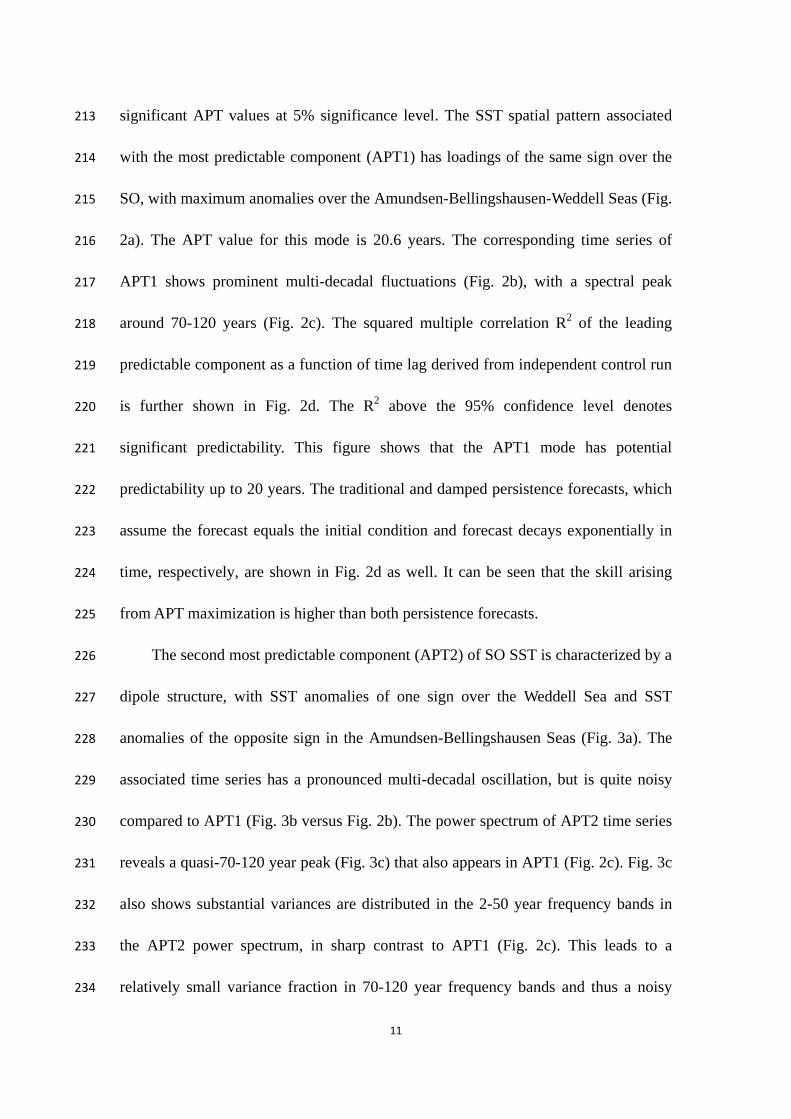
significant APT values at 5% significance level. The SST spatial pattern associated 213
with the most predictable component (APT1) has loadings of the same sign over the 214
SO, with maximum anomalies over the Amundsen-Bellingshausen-Weddell Seas (Fig. 215
2a). The APT value for this mode is 20.6 years. The corresponding time series of 216
APT1 shows prominent multi-decadal fluctuations (Fig. 2b), with a spectral peak 217
around 70-120 years (Fig. 2c). The squared multiple correlation R2 of the leading 218
predictable component as a function of time lag derived from independent control run 219
is further shown in Fig. 2d. The R2 above the 95% confidence level denotes 220
significant predictability. This figure shows that the APT1 mode has potential 221
predictability up to 20 years. The traditional and damped persistence forecasts, which 222
assume the forecast equals the initial condition and forecast decays exponentially in 223
time, respectively, are shown in Fig. 2d as well. It can be seen that the skill arising 224
from APT maximization is higher than both persistence forecasts. 225
The second most predictable component (APT2) of SO SST is characterized by a 226
dipole structure, with SST anomalies of one sign over the Weddell Sea and SST 227
anomalies of the opposite sign in the Amundsen-Bellingshausen Seas (Fig. 3a). The 228
associated time series has a pronounced multi-decadal oscillation, but is quite noisy 229
compared to APT1 (Fig. 3b versus Fig. 2b). The power spectrum of APT2 time series 230
reveals a quasi-70-120 year peak (Fig. 3c) that also appears in APT1 (Fig. 2c). Fig. 3c 231
also shows substantial variances are distributed in the 2-50 year frequency bands in 232
the APT2 power spectrum, in sharp contrast to APT1 (Fig. 2c). This leads to a 233
relatively small variance fraction in 70-120 year frequency bands and thus a noisy 234

12
APT2 time series. The R2 of this second most predictable component indicates a 235
potential predictability up to 5 years (Fig. 3d), which is much shorter than the first 236
predictable mode due to noisy characteristics. The APT2 predictability is only slightly 237
higher than the persistence forecasts (Fig. 3d), suggesting that the skill mainly arises 238
from the SST persistence. 239
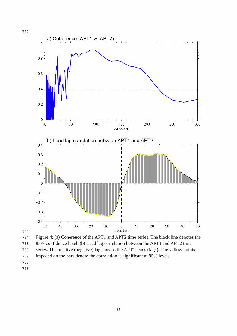
The coherent spectrum of APT1 and APT2 time series shows high coherences 240
over their common peak period 70-120yr (Fig.4a), suggesting that the leading two 241
predictable components may have the same ocean origin. To confirm our hypothesis, 242
we conduct a lead lag correlation analysis between these two time series (Fig. 4b). As 243
expected, the simultaneous correlation is zero due to the orthogonality of the APT 244
decomposition. Significant positive (negative) correlations are found when the APT1 245
leads (lags) APT2 by 10-30 years. These lead and lag times account for approximately 246
a quarter of the APT1/APT2 period (70-120 year). These phenomena imply that the 247
two predictable components are very likely quadrature related. 248
4. Ocean origin of high decadal predictability of SO SST 249
a. Climate fluctuations associated with leading predictable modes 250
To understand the physical processes associated with the leading predictable 251
components, we regress several important variables onto the APT1 and APT2 time 252
series, respectively (Fig. 5 and 6). Fig. 5a exhibits the surface net heat flux and mixed 253
layer depth (MLD) anomalies associated with the APT1 time series. The SO 254
experiences broad negative heat flux anomalies that tend to damp positive surface 255
temperature anomalies. This implies that the uniform SO SST warming in APT1 256

13
originates from the ocean dynamics, instead of atmosphere forcing. The MLD change 257
shown in Fig. 5a displays a strong positive anomaly over the Weddell Sea, indicating 258
strong deep convection there. Note that the long term mean global meridional 259
overturning circulation (GMOC) has a negative value south of 60oS, which represents 260
an anticlockwise cell that denotes the strength of Antarctic Bottom water (AABW) 261
formation as well as deep convection (Fig. 7a). Fig. 5b shows prominent negative 262
GMOC anomalies south of 20oS, suggesting a strengthening and northward extension 263
of the AABW Cell. In the mean state the subsurface is warmer than the surface in the 264
region of the SO. Therefore, the spin up of AABW cell drives a subsurface-surface 265
temperature dipole in the SO, with a cooling anomaly in the subsurface and a 266
warming anomaly at the surface (Fig. 5c) that corresponds to a decrease of Antarctic 267
sea ice (Fig. 5d). The surface wind is characterized by a zonally-oriented anticyclone 268
around 40oS-60
oS band, which is very likely due to local SST feedback (Zhang et al. 269
2016). These ocean and atmosphere variabilities associated with the APT1 mode are 270
consistent with the SO centennial climate variability found in Kiel Climate Model 271
(Latif et al. 2013). 272
The heat flux and MLD anomalies associated with the APT2 time series show 273
opposite signs with the APT1 (Fig. 6a versus Fig. 5a), suggesting a weakening of deep 274
convection over the Weddell Sea. Accordingly, the GMOC anomaly shows a spin 275
down of AABW cell (Fig. 6b). Compared to APT1, the GMOC change is relatively 276
weak and mainly confined south of 60oS (Fig. 5b versus Fig. 6b). The associated 277
zonal mean temperature shows a weak cold surface-warm subsurface dipole structure 278

14
over the SO (Fig. 6c). In contrast to the uniform sea ice response in APT1, the sea ice 279
change associated with APT2 exhibit a dipole pattern, with sea ice increase in the 280
Weddell Sea and sea ice decrease over the Amundsen-Bellingshausen Seas (Fig. 6d). 281
The sea ice anomaly over the Amundsen-Bellingshausen Seas is not only related to 282
the SST anomalies but also linked with the surface wind. As shown in Fig. 6d, there is 283
an anticyclonic wind around 160o-40
oW over the SO, which corresponds to a 284
northwest wind anomaly over the Amundsen-Bellingshausen Seas. The northwest 285
wind favors poleward warm temperature advection and thus a decrease of sea ice 286
there. 287
The above regression analyses suggest that the leading two predictable 288
components of SO SST are very likely to be associated with deep convection changes. 289
To test this hypothesis, we examine the SO deep convection characteristics in the 290
CM2.1 model. As mentioned above, we use the AABW cell anomaly to represent the 291
SO deep convection fluctuations. The strength of the AABW cell each year is defined 292
as the minimum value of the streamfunction south of 60oS (Fig. 7a). Note that if the 293
AABW cell index is a negative anomaly, which means a strong overturning cell. The 294
time series of AABW cell index (Fig. 7b) has pronounced multi-decadal variabilities 295
at 70-120yr time scales (Fig. 7c) which coincide with the typical period peaks of 296
APTs (Fig. 7c versus Fig. 2c and Fig. 3c). We also show in Fig. 7d the lead lag 297
correlation between the AABW cell index and APT1 time series. It shows a negative 298
correlation as low as -0.6 when the AABW leads the APT1 by about 5 years. Since the 299

15
APT1 and APT2 time series are in quadrature, significant correlations are also found 300
between the AABW index and APT2 with some time lags (not shown). 301
b. Southern Ocean multi-decadal variability 302
To further confirm the close relationship between the leading predictable 303
components and SO deep convection, we show in Fig. 8 the multi-decadal cycle of 304
AABW cell. The AABW cell cycle is obtained by the lagged regression of GMOC 305
anomalies upon the AABW cell index. To focus on multi-decadal variability, all data 306
are first 10-yr averaged prior to regression. At a lag of 0yr, the AABW cell is in its 307
mature positive phase, with a maximum increase south of 60oS and a northward 308
extension to 40oS (Fig. 8a). We characterize the evolution of the AABW cell cycle by 309
the regression coefficients at various lags. As we move forward from lag 0, the 310
GMOC anomalies south of 60oS gradually weaken, while the northward extension 311
becomes stronger and stronger (Fig. 8b-d). The GMOC negative anomalies extend to 312
about 20oN at a lag of 15yr (Fig. 8d). At a lag of 20yr, a positive GMOC anomaly 313
emerges south of 60oS. This positive GMOC anomaly then intensifies and gradually 314
spreads northward, which in turn weakens the negative GMOC anomaly in the north 315
(Fig. 8e-j). At a lag of 45yr, the AABW phase is totally flipped and reaches its mature 316
negative phase (Fig. 8j). A close examination finds that the spatial structure of quasi 317
mature phase of AABW cell (Fig. 8a, b) closely resembles the GMOC anomalies 318
associated with the APT1 (Fig. 5b). Similarly, the transition phase of AABW cycle 319
(Fig. 8f) matches with the GMOC anomalies associated with the APT2 very well (Fig. 320
6b). 321

16
We show in Fig. 9 the multidecadal SST cycle associated with the deep 322
convection. During the AABW cell mature positive phase, the SO experiences broad 323
warming anomalies, with maximum values over the Weddell Sea (Fig. 9a, b). The 324
warm SST over the SO corresponds to a zonally-oriented anticyclone wind, with 325
easterly anomalies around 40oS and westerly anomalies at 75
oS. We note that the 326
mature phase of the SO SST cycle here is in good agreement with the SST pattern in 327
APT1 (Fig. 9a, b versus Fig. 2a). Accompanied with the AABW cell weakening south 328
of 60oS (Fig. 8a-d), the positive SST anomalies over the Weddell Sea gradually 329
weaken (Fig. 9a-d). At the same time, the Southeast Pacific SST warming gradually 330
spreads to the equator through the fast positive wind-evaporation-SST (WES) 331
feedback and slow weakening of subtropical cell (e.g., Zhang et al. 2011) (Fig. 9a-d). 332
Once the warm SST anomaly reaches the equatorial eastern Pacific, it triggers the 333
tropical positive Bjerknes feedback to further amplify the initial SST anomaly. The 334
warm SST anomaly over the tropical Pacific induces the positive phase of Pacific 335
North America (PNA) teleconnection (e.g., Horel and Wallace 1981) and Pacific 336
South America (PSA) teleconnection (Mo and Higgins 1997) as well. The PNA 337
teleconnection leads to a PDO-like (e.g. Zhang and Delworth, 2015, 2016) SST 338
pattern over the North Pacific with cold SST anomalies over the western and central 339
Oceans (Fig. 9b-d). The PSA teleconnection induces a wavenumber 3 in the 340
mid-latitude, with an anticyclonic circulation over the Amundsen-Bellingshausen Seas 341
that favors warm poleward advection and thus warm SST there (Fig. 9c-d). At a lag of 342
20yr, a cooling SST anomaly appears in the Weddell Sea (Fig. 9e) resulting from the 343

17
emergence of a negative AABW cell shown in Fig. 8e. The SST over the SO is 344
characterized by a dipole pattern at this moment, with a warm SST in the 345
Amundsen-Bellingshausen Seas and a cold SST in the Weddell Sea. The negative SST 346
anomaly in the Weddell Sea further grows in the Weddell Sea and then extends to the 347
entire SO (Fig. 9f-j). At lags of 35-45yr, the SO is almost covered by the negative SST 348
anomalies (Fig. 9h-j), which reaches to the opposite phase of deep convection. We 349
note again that the transition phase of SO SST cycle matches very well with the SST 350
pattern in APT2 (Fig. 9f versus Fig. 3a). These SST pattern similarities suggest that 351
the leading two predictable components of SO SST originate from the internal 352
multi-decadal cycle of SO deep convection. The first component arises from the quasi 353
mature phase of deep convection, while the second component is contributed from the 354
transition phase of deep convection. 355
The associated sea ice and subsurface temperature variabilities (Fig. 10, 11) are 356
physically consistent with our previous analyses. The sea ice primarily follows the 357
SST changes, with a cold (warm) SST anomaly corresponding to a sea ice increase 358
(decrease). Thus, the mature positive phase sea ice at lag 0yr is characterized by a sea 359
ice decrease over the SO (Fig. 10a, b), whereas the transition phase sea ice at lag 25yr 360
exhibits a sea ice decrease in the Amundsen-Bellingshausen Seas and a sea ice 361
increase in the Weddell Sea (Fig. 10f). These sea ice characteristics are consistent 362
with the sea ice anomalies associated with the APT1 and APT2 (Fig. 10a, b versus 363
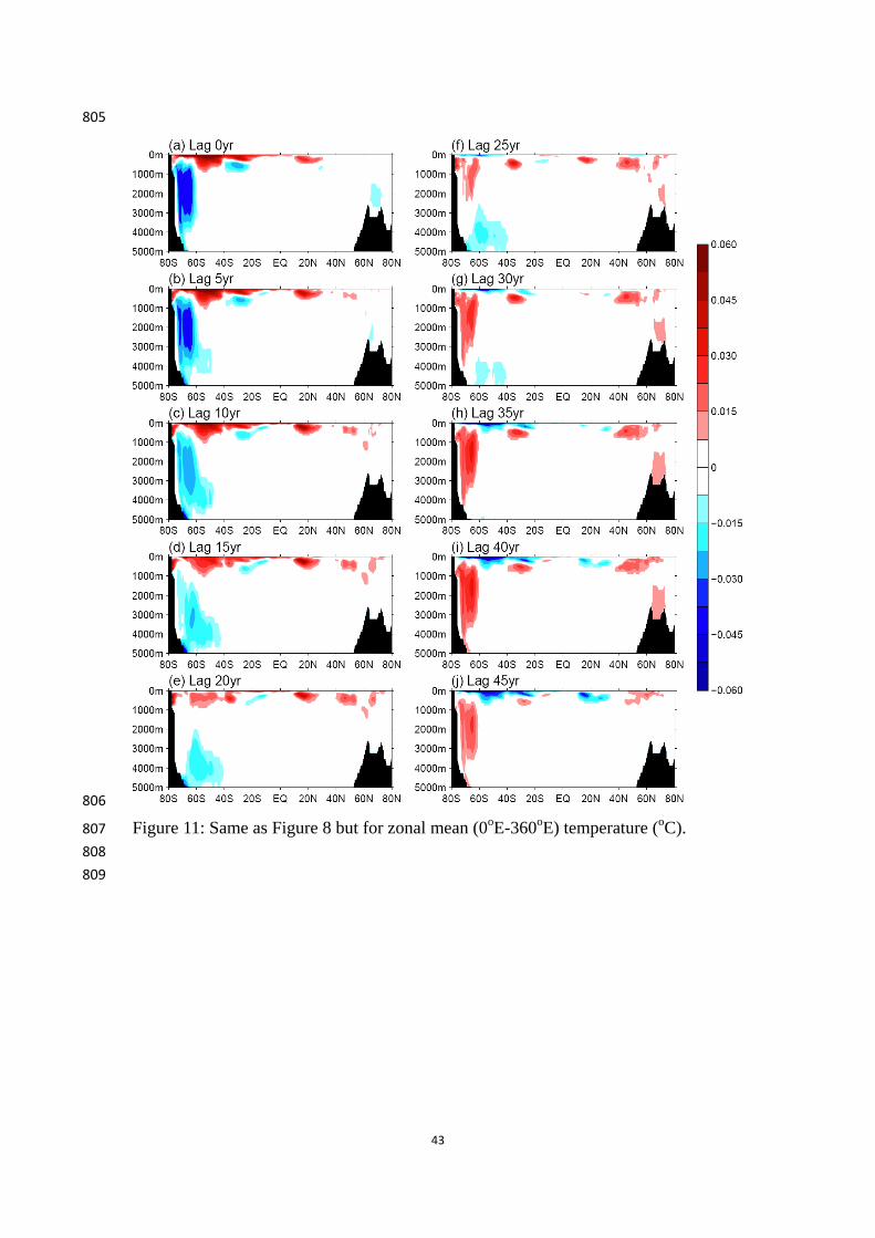
Fig. 5d; Fig. 10e, f versus Fig. 6d). Fig. 11 shows the multidecadal zonal mean 364
temperature cycle. As expected, the temperature response agrees with the deep 365

18
convection change (Fig. 11 versus Fig. 8). The spin up (spin down) of AABW cell 366
brings subsurface warm water to the surface, thereby leading to a warm (cold) SST in 367
the surface and a cold (warm) temperature in the subsurface. The dipole temperature 368
weakens as the AABW cell spins down and vice versa. The temperature dipole 369
structure becomes quite weak during the deep convection transition phase as 370
compared to the mature phase (Fig. 11f versus Fig. 11a). Again, these zonal mean 371
temperature anomalies in the mature and transition phases match with the temperature 372
responses in APT1 and APT2, respectively (Fig. 11a, b versus Fig. 5c; Fig. 11f versus 373
Fig. 6c). 374
We note that the most predictable SST (APT1) time series over the SO lags the 375
AABW cell index by about 5 years (Fig. 7d). The delayed SST response primarily 376
arises from the slow adjustment of the ocean that consists of advection/wave 377
propagation (Zhang and Delworth 2016), which is also seen in the CM2.1 fully 378
coupled control run. Fig. 12a exhibits the SO (50o-75
oS, 0
o-360
oE) area averaged SST 379
time series, the Weddell Sea (75-55oS, 52
oW-30
oE) area averaged SST time series as 380
well as the AABW cell index. Their lead-lag correlations are shown in Fig. 12b. All 381
three indices have pronounced multi-decadal fluctuations and they are highly 382
correlated. The AABW cell index is simultaneously correlated with the local (Weddell 383
Sea) SST due to strong deep convection there. In contrast, the maximum correlation 384
between the AABW cell index and remote SO SST occurs when the AABW cell leads 385
by about 5 years (Fig. 12b). The delayed SST response is again related to the slow 386
ocean adjustment. 387

19
c. Mechanisms contributing to SO multi-decadal variability 388
The main driver of the deep convection in CM2.1 model is the heat reservoir at 389
mid-depth and its recharge process, which have great similarities with that in Kiel 390
Climate model (Martin et al. 2013). Fig. 13a shows the time evolution of annual mean 391
vertical temperature anomaly averaged over the Weddell Sea. The temperature 392
anomaly is relative to a composite of 30 years of two major convection periods (year 393
2950-2980 and year 3020-3050). During active convection, the temperature 394
distribution is almost homogeneous over the entire water column. However, the heat 395
tends to accumulate at mid-depth when the convection stops. The heat spreads over 396
time, warms the entire water column below 300m, destabilizes the ocean stratification, 397
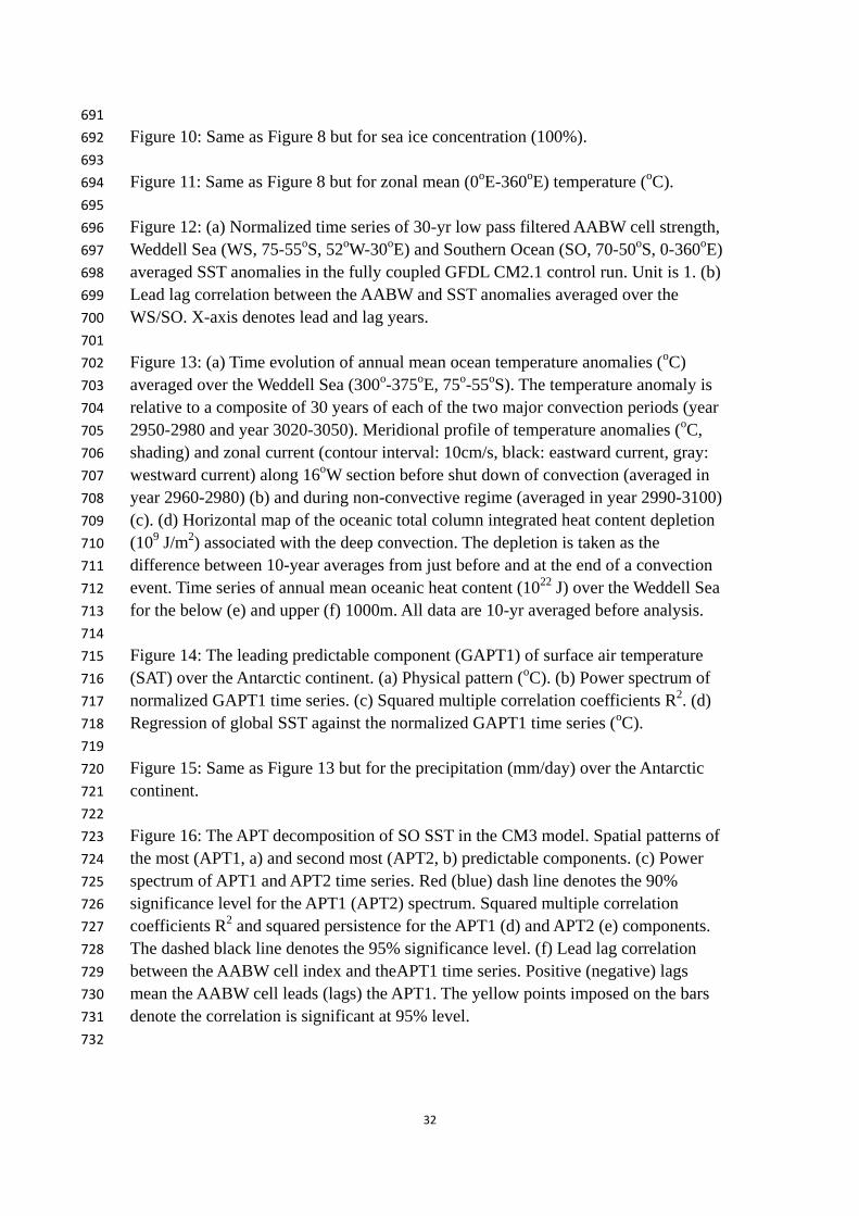
and eventually triggers the occurrence of deep convection. 398
The heat at mid-depth over the Weddell Sea primarily comes from the northern 399
subtropics. Before the shutdown of deep convection, the westward return flow in the 400
southern branch of the Weddell Gyre effectively drags heat into the Weddell Sea (Fig. 401
13b). This strong barotropic clockwise gyre exists over almost the entire water 402
column and its’ strength is strongly associated with the deep convection itself due to 403
interactions between the AABW outflow and topography (Zhang and Delworth 2016). 404
The gyre still exits when the convection spins down, albeit with a weak amplitude 405
(Fig. 13c). 406
The convection shutdown is the depletion of heat reservoir at mid-depth (Fig. 13a). 407
The deep convection leads to a heat depletion in the entire Atlantic and Indian Ocean 408
Basins (Fig. 13d). By separating the heat content into upper 1000m and deep 409

20
components, we can see the deep ocean loses and the upper ocean gains heat when the 410
convection occurs and vice versa (Fig. 13e, f). Moreover, the deep ocean heat content 411
dominates the whole water column heat changes. Most of the heat lost during the deep 412
convection is imported into the Weddell Sea by the westward return flow of the 413
Weddell Gyre (Fig. 13b). 414
In brief, the recharge/discharge processes of heat reservoir at mid-depth are the 415
main mechanism driving multi-decadal variability over the SO, although other 416
processes such as heat flux loss to the atmosphere, freshwater change in the surface 417
and sea ice melt/formation could slightly modulate this variability (not shown). The 418
timescale of the cycle is largely determined by the recharge and discharge processes 419
of the heat reservoir over the Weddell Sea. The heat content variation there is 420
associated with the warm water in the northern subtropics and the Weddell Gyre 421
strength. 422
5. Climate impacts 423
In this section, we examine the potential multiyear predictability of surface air 424
temperature (SAT) and precipitation over the Antarctic continent. We find the 425
multiyear predictability of land variables using land predictor itself is lower than the 426
predictability using global SST (not shown). This suggests that the land predictability 427
on interannual-to-decadal time scales is primarily driven by SST (Hoerling and 428
Kumar 2003; Held et al. 2005). Thus, we use a generalized APT method (GAPT) (Jia 429
and DelSole 2011), which is similar to the standard APT described in section 2, except 430
21
that the predictor and predictand are two different variables. Here the predictor is 431
global SST, while the predictand is SAT or precipitation. 432
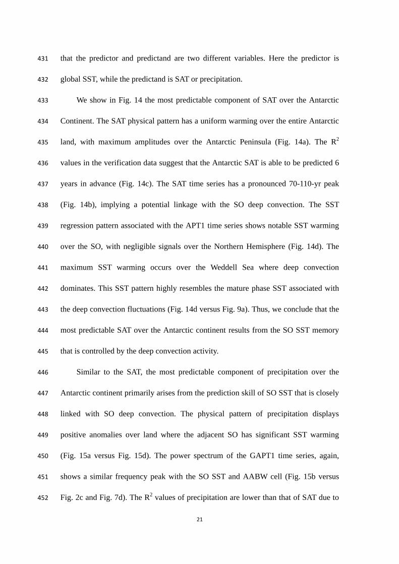
We show in Fig. 14 the most predictable component of SAT over the Antarctic 433
Continent. The SAT physical pattern has a uniform warming over the entire Antarctic 434
land, with maximum amplitudes over the Antarctic Peninsula (Fig. 14a). The R2 435
values in the verification data suggest that the Antarctic SAT is able to be predicted 6 436
years in advance (Fig. 14c). The SAT time series has a pronounced 70-110-yr peak 437
(Fig. 14b), implying a potential linkage with the SO deep convection. The SST 438
regression pattern associated with the APT1 time series shows notable SST warming 439
over the SO, with negligible signals over the Northern Hemisphere (Fig. 14d). The 440
maximum SST warming occurs over the Weddell Sea where deep convection 441
dominates. This SST pattern highly resembles the mature phase SST associated with 442
the deep convection fluctuations (Fig. 14d versus Fig. 9a). Thus, we conclude that the 443
most predictable SAT over the Antarctic continent results from the SO SST memory 444
that is controlled by the deep convection activity. 445
Similar to the SAT, the most predictable component of precipitation over the 446
Antarctic continent primarily arises from the prediction skill of SO SST that is closely 447
linked with SO deep convection. The physical pattern of precipitation displays 448
positive anomalies over land where the adjacent SO has significant SST warming 449
(Fig. 15a versus Fig. 15d). The power spectrum of the GAPT1 time series, again, 450
shows a similar frequency peak with the SO SST and AABW cell (Fig. 15b versus 451
Fig. 2c and Fig. 7d). The R2 values of precipitation are lower than that of SAT due to 452

22
the noisy characteristics of precipitation (Fig. 14c versus Fig. 15c). However, the 453
potential predictability of precipitation can still be up to 4 years (Fig. 15c). 454
6. Summary, discussion and conclusion 455
By taking advantage of the GFDL CM2.1 4000-yr control run integration, we 456
investigate the potential decadal predictability of SO SST in the present paper. We use 457
a new statistical optimization technique, called APT analysis (DelSole and Tippett 458
2009a, b), to identify the leading predictable components of SO SST on decadal time 459
scales. The APT analysis maximizes an integrated prediction variance obtained from a 460
linear regression model, in which both the predictor and predictand are SST. Note that 461
the long term control integration does not include anthropogenic forcing or changes in 462
natural forcing from volcanoes or interannual variations of solar irradiance. The 463
potential predictability shown here is therefore purely from internal variability. 464
The most predictable component of SO SST can be predicted in an independent 465
verification data by a linear regression model, with significant skill up to 20 years. 466
The predictable pattern has a uniform SST sign over the SO, with maximum values 467
over the Amundsen-Bellingshausen-Weddell Seas. The associated APT time series has 468
a 70-120-yr spectral peak. This predictable pattern is closely related to the mature 469
phase of the SO internal variability that originates from deep convection fluctuations. 470
In the CM2.1 model, deep convection mainly occurs over the Weddell Sea and has 471
multidecadal fluctuations on a 70-120-yr time scale. This multi-decadal timescale 472
selection is largely associated with the discharge and recharge processes of heat 473
reservoir in the deep ocean. Slow subsurface ocean processes provide long time scales 474

23
that give rise to decadal predictability of SO SST. The SO SST has significant climate 475
impacts on the SAT and precipitation over the Antarctic continent. The SAT and 476
precipitation can be potentially predictable up to 6yr and 4yr in advance, respectively. 477
These multiyear prediction skills arise from the SO SST, which is again attributed to 478
the internal deep convection fluctuations over the Weddell Sea. 479
The second most predictable component of SO SST is characterized by a dipole 480
structure, with SST anomalies of one sign over the Weddell Sea and SST anomalies of 481
the opposite sign over the Amundsen-Bellingshausen Seas. This component has 482
statistically significant prediction skill for 6 years based on a linear regression model. 483
A close examination reveals that this dipole mode primarily arises from the transition 484
phase of the dominant pattern of SO internal variability. Again, the slow ocean 485
memory associated with the SO deep convection provides the multiyear prediction 486
skill of this second most predictable component. Interestingly, this second component 487
corresponds to a sea ice dipole structure over the Amundsen-Bellingshausen-Weddell 488
Seas, which somewhat resembles the observed sea ice trend in recent years (e.g., Li et 489
al. 2014). The associated surface wind over the SO characterized by a cyclone (or 490
anticyclone) around 160o-40
oW favors sea ice dipole formation, which is also 491
consistent with what was found in observation. These similarities provide a 492
hypothesis that some prominent trends observed during the recent decades in the 493
Southern Hemisphere may have some contributions from internal variability in the SO 494
that is strongly associated with deep convection fluctuations. 495

24
In order to provide some perspective on the robustness of our results, we perform 496
the same APT diagnostics on a long control integration of a different GFDL climate 497
model, CM3 (Donner et al., 2011). The CM3 model has an ocean component that is 498
quite similar to CM2.1, but the atmospheric component of CM3 has substantial 499
differences from CM2.1. Similar to CM2.1, the most predictable SST pattern in CM3 500
displays a uniform sign over the SO, while the second most predictable SST pattern 501
shows a dipole structure (Fig. 16a, b). The maximum SST centers associated with 502
these two modes are primarily over continental shelfs of the Weddell and Ross Seas 503
(Fig. 16a and b), which are somewhat different from CM2.1 (Fig. 2 and 3). These SST 504
center differences are largely associated with the deep convection position in two 505
models (not shown). The SO deep convection mainly occurs in the Weddell Sea in 506
CM2.1 model, including both open oceans and continental shelf. In contrast, the deep 507
convection in CM3 model takes places in continental shelfs of the Weddell and Ross 508
Seas. 509
The power spectrum of APT1 and APT2 time series in CM3 model shows 510
prominent spectrum peaks around 300 years, which are longer than that in CM2.1 511
model (Fig. 16c versus Fig. 2c and 3c). This leads to a long persistence time of SST 512
and therefore a long predictability skill, as presented in Fig. 16d and e. The predictive 513
skill can be up to 30 years for APT1 component and 10 years for APT2 mode. In 514
agreement with that in the CM2.1 model, these leading predictable components are 515
found to be closely linked with the SO deep convection fluctuations (Fig. 16f). 516

25
Our diagnostic approaches for the decadal predictability of SO SST in the current 517
paper suggest that if we could correctly initialize the SO deep convection in the 518
numerical forecast model, the future evolution of SO SST and its associated climate 519
impacts might be predictable on decadal scales. Such predictions would ideally be 520
performed using models with simulations of the SO that are as realistic as possible. In 521
addition, enhanced ocean observations, particularly subsurface observations over the 522
far SO, are also needed to characterize the state of the SO. An important caveat is that 523
the realism of model's simulation of the SO will impact how relevant such potential 524
predictive skill is for predictions of the real climate system. The decadal prediction 525
skill of SO SST based on real decadal hindcasts/forecasts is currently under 526
investigation and will be the topic of a forthcoming paper. 527
528
Acknowledgement: 529
We are grateful to Soyna Legg and Carolina O. Dufour for their constructive 530
comments on an early version of the paper. The work of T. Delworth is supported as a 531
base activity of NOAA’s Geophysical Fluid Dynamics Laboratory. L. Zhang and L. 532
Jia are supported through Princeton University under block funding from 533
NOAA/GFDL. 534
535

26
Reference: 536
537
Boer, G. J., 2004: Long time-scale potential predictability in an ensemble of coupled 538
climate models. Climate Dyn., 23, 29-44. 539
Boer, G. J., 2011: Decadal potential predictability of twenty-first century climate. 540
Climate Dyn., 36, 1119-1133. 541
Boer, G. J., and S. J. Lambert, 2008: Multi-model decadal potential predictability of 542
precipitation and temperature. Geophys. Res. Lett., 35, L05706, 543
doi:10.1029/2008GL033234. 544
Cane, M. A., 2010: Climate science: Decadal predictions in demand. Nat. Geosci., 3, 545
231–232. 546
Cavalieri, D. J., and C. L. Parkinson, 2008: Antarctic sea ice variability and trends, 547
1979-2006. J. Geophys. Res., 113, C07004, doi:10.1029/2007JC004564. 548
Chen, X., and K.-K. Tung, 2014: Varying planetary heat sink led to global-warming 549
slowdown and acceleration. Science, 345, 897–903. 550
Comiso, J. C., and F. Nishio, 2008: Trends in the sea ice cover using enhanced and 551
compatible AMSR-E, SSM/I, and SMMR data. J. Geophys. Res., 113, C02S07, 552
doi:10.1029/2007JC004257. 553
DelSole, T., and M. K. Tippett, 2009a: Average predictability time. Part I: Theory. J. 554
Atmos. Sci., 66, 1172–1187. 555
DelSole, T. , and M. K. Tippett, 2009b: Average predictability time. Part II: Seamless 556
diagnosis of predictability on multiple time scales. J. Atmos. Sci., 66, 1172–1187. 557
DelSole, T., L. Jia, and M. K. Tippett, 2013: Decadal prediction of observed and 558

27
simulated sea surface temperatures. Geophys. Res. Lett., 40, 2773–2778, 559
doi:10.1002/grl.50185. 560
Delworth, T. L., and Coauthors, 2006: GFDL’s CM2 global coupled climate models. 561
Part I: Formulation and simulation characteristics. J. Climate, 19, 643–674. 562
Donner, L. J., and coauthors, 2011: The dynamical core, physical parameterizations, 563
and basic simulation characteristics of the atmospheric component AM3 of the 564
GFDL global coupled model CM3. J. Climate, 24, 3484-3519, doi: 565
10.1175/2011JCLI3955.1. 566
Held, I. M., T. L. Delworth, J. Lu, K. L. Findell, and T. R. Knutson, 2005: Simulation 567
of Sahel drought in the 20th and 21st centuries. Proc. Natl. Acad. Sci., 102, 568
17891-17896. 569
Hoerling, M., and A. Kumar, 2003: The perfect ocean for drought. Science, 299, 691–570
694. 571
Horel, J. D., and J. M. Wallace, 1981: Planetary-scale atmospheric phenomena 572
associated with the Southern Oscillation. Mon. Wea. Rev., 109, 813–829. 573
Jia, L., and T. DelSole, 2011: Diagnosis of multiyear predictability on continental 574
scales. J. Climate, 24, 5108–5124. 575
Keenlyside, N. S., M. Latif, J. Jungclaus, L. Kornblueh, and E. Roeckner, 2008: 576
Advancing decadal-scale climate prediction in the North Atlantic sector. Nature, 577
453, 84-88. 578
Latif, M., T. Martin, and W. Park, 2013: Southern Ocean sector centennial climate 579
variability and recent decadal trends. J. Climate, 26, 7767–7782, 580

28
doi:10.1175/JCLI-D-12-00281.1. 581
Martin, T., W. Park and M. Latif, 2013: Multi-centennial variability controlled by 582
Southern Ocean convection in the Kiel Climate Model. Clim. Dyn., 40, 583
2005-2022. 584
Msadek, R., and Coauthors, 2014: Predicting a decadal shift in North Atlantic climate 585
variability using the GFDL forecast system. J. Climate, 27, 6472-6496. 586
Meehl, G. A., and H. Teng, 2012: Case studies for initialized decadal hindcasts and 587
predictions for the Pacific region. Geophys. Res. Lett., 39, L22705, 588
doi:10.1029/2012GL053423. 589
Mo, K. C., and R. W. Higgins, 1997: The Pacific–South American mode and tropical 590
convection during the Southern Hemisphere winter. Mon. Wea. Rev., 126, 1581–591
1596. 592
Mochizuki, T., and Coauthors, 2010: Pacific decadal oscillation hindcasts relevant to 593
near-term climate prediction. Proc. Natl. Acad. Sci., 107, 1833-1837. 594
Newman, M., 2007: Interannual to decadal predictability of tropical and North Pacific 595
sea surface temperatures. J. Climate, 20, 2333-2356. 596
Polvani, L. M., and K. L. Smith, 2013: Can natural variability explain observed 597
Antarctic sea ice trends? New modeling evidence from CMIP5. Geophys. Res. 598
Lett., 40(12), 3195–3199, doi: 10.1002/grl.50578. 599
Pohlmann, H., M. Botzet, M. Latif, A. Roesch, M. Wild, and P. Tschuck, 2004: 600
Estimating the decadal predictability of a coupled AOGCM. J. Climate, 17, 601
4463–4472. 602

29
Purkey, S. G., and G. C. Johnson, 2010: Warming of global abyssal and deep Southern 603
Ocean waters between the1990s and 2000s: Contributions to global heat and sea 604
level rise budgets. J. Climate, 23, 6336–6351. 605
Purkey, S. G., and G. C. Johnson, 2012: Global contraction of Antarctic Bottom Water 606
between the 1980s and 2000s. J. Climate, 25, 5830–5844. 607
Purich, A., W. Cai, M. H. England and T. Cowan, 2016: Evidence for link between 608
modelled trends in Antarctic sea ice and underestimated westerly wind changes. 609
Nature Communications, 7, 10409, doi:10.1038/ncomms10409. 610
Robson, J. I., R. T. Sutton, and D. M. Smith, 2012: Initialized decadal predictions of 611
the rapid warming of the North Atlantic Ocean in the mid 1990s. Geophys. Res. 612
Lett., 39, L19713, doi:10.1029/2012GL053370. 613
Smith, T. M., and R. W. Reynolds, 2004: Improved extended reconstruction of SST 614
(1854-1997). J. Climate, 17, 2466-2477. 615
Smith, D. M., S. Cusack, A. W. Colman, C. K. Folland, G. R. Harris, and J. M. 616
Murphy, 2007: Improved surface temperature prediction for the coming decade 617
from a global climate model. Science, 317, 796-799. 618
Wang, G., and D. Dommenget, 2016: The leading modes of decadal SST variability in 619
the Southern Ocean in CMIP5 simulations. Clim. Dyn., 47, 1775-1792. 620
Yang, X., and Coauthors, 2013: A predictable AMO-like pattern in the GFDL fully 621
coupled ensemble initialized and decadal forecasting system. J. Climate, 26, 622
650-661. 623
Yeager, S. G., A. Karspeck, G. Danabasoglu, J. Tribbia, and H. Teng, 2012: A decadal 624

30
prediction case study: Late twentieth-century North Atlantic Ocean heat content. 625
J. Climate, 25, 5173–5189. 626
Zunz, V., H. Goosse, and F. Massonnet, 2013: How does internal variability influence 627
the ability of CMIP5 models to reproduce the recent trend in Southern Ocean sea 628
ice extent? Cryosphere, 7, 451-468. 629
Zanna, L., P. Heimbach, A. M. Moore, and E. Tziperman, 2012: Upper-ocean singular 630
vectors of the North Atlantic climate with implications for linear predictability 631
and variability. Quart. J. Roy. Meteor. Soc., 138, 500–513, doi:10.1002/qj.937. 632
Zhang, L., L. W, and J. Zhang, 2011: Simulated response to recent freshwater flux 633
change over the gulf stream and its extension: coupled Ocean-Atmosphere 634
adjustment and Atlantic-Pacific Teleconnection. J. Climate., 24(15), 3971-3988. 635
Zhang, L., and T. L. Delworth, 2015: Analysis of the characteristics and mechanisms 636
of the Pacific Decadal Oscillation in a suite of coupled models from the 637
Geophysical Fluid Dynamics Laboratory. J. Climate, 28, 7678–7701. 638
Zhang, L., and T. L. Delworth, 2016: Simulated response of the Pacific decadal 639
oscillation to climate change. J. Climate, 29, 5999–6018. 640
Zhang, L., T. L. Delworth and F. Zeng, 2016: The impact of multidecadal Atlantic 641
meridional overturning circulation variations on the Southern Ocean. Clim. Dyn., 642
doi:10.1007/s00382-016-3190-8. 643
Zhang, L., and T. L. Delworth 2016: Impact of the Antarctic bottom water formation 644
on the Weddell Gyre and its northward propagation characteristics in GFDL 645
model. Journal of Geophysical Research: Oceans, 121(8), 5825-5846. 646

31
647
Figure Captions: 648
649
Figure 1: Spatial patterns of potential predictability variance fraction (ppvf) for 5-yr 650
(a), 11-yr (b) and 25-yr (c) mean SST in GFDL CM2.1 control run. 651
652
Figure 2: The leading predictable component (APT1) of Southern Ocean (SO) SST in 653
GFDL CM2.1 model. (a) Spatial pattern (oC). (b) Normalized time series. (c) Power 654
spectrum of time series (black line). The blue line denotes the 90% confidence level 655
based on red noise null hypothesis (d) Squared multiple correlation coefficients R2. 656
The dashed black line denotes the 95% significance level. 657
658
Figure 3: Same as Figure 2 but for the second most predictable component (APT2). 659
660
Figure 4: (a) Coherence of the APT1 and APT2 time series. The black line denotes the 661
95% confidence level. (b) Lead lag correlation between the APT1 and APT2 time 662
series. The positive (negative) lags means the APT1 leads (lags). The yellow points 663
imposed on the bars denote the correlation is significant at 95% level. 664
665
Figure 5: Regression of (a) mixed layer depth (m, shading)/ net heat flux (Contour 666
interval is 1W/m2. Black solid lines denote the atmosphere heating the ocean, while 667
the grey dash lines denote the ocean losing heat to the atmosphere), (b) global 668
meridional overturning circulation (GMOC, Sv), (c) zonal mean (0o-360
oE) 669
temperature (oC) and (d) sea ice concentration (100%)/surface wind (m/s) upon the 670
normalized APT1 time series. Shown are only regions where the regression is 671
significant at 95% confidence level. 672
673
Figure 6: Same as Figure 5 but upon the normalized APT2 time series. 674
675
Figure 7: Characteristics of internal deep convection over the SO in GFDL CM2.1 676
model. (a) Long term mean GMOC (Sv). Red (blue) color denotes clockwise 677
(anti-clockwise) cell. (b) Normalized time series of Antarctic Bottom Water (AABW) 678
Cell index which is defined as the minimum value of GMOC value south of 60oS. (c) 679
Power spectrum of AABW cell index. (d) Lead lag correlation between the AABW 680
cell index and the most predictable component of SO SST (APT1). Positive (negative) 681
lags mean the AABW cell leads (lags) the APT1. 682
683
Figure 8: Lagged regression of GMOC anomalies against the normalized AABW cell 684
index in GFDL CM2.1 model. Unit is Sv. All data are 10-yr averaged before 685
regression. Shown are only regions where the regression is significant at 95% 686
confidence level. 687
688
Figure 9: Same as Figure 8 but for the SST (shading) and surface wind stress (vector). 689
Units are oC for SST and N/m
2 for wind stress. 690
32
691
Figure 10: Same as Figure 8 but for sea ice concentration (100%). 692
693
Figure 11: Same as Figure 8 but for zonal mean (0oE-360
oE) temperature (
oC). 694
695
Figure 12: (a) Normalized time series of 30-yr low pass filtered AABW cell strength, 696
Weddell Sea (WS, 75-55oS, 52
oW-30
oE) and Southern Ocean (SO, 70-50
oS, 0-360
oE) 697
averaged SST anomalies in the fully coupled GFDL CM2.1 control run. Unit is 1. (b) 698
Lead lag correlation between the AABW and SST anomalies averaged over the 699
WS/SO. X-axis denotes lead and lag years. 700
701
Figure 13: (a) Time evolution of annual mean ocean temperature anomalies (oC) 702
averaged over the Weddell Sea (300o-375
oE, 75
o-55
oS). The temperature anomaly is 703
relative to a composite of 30 years of each of the two major convection periods (year 704
2950-2980 and year 3020-3050). Meridional profile of temperature anomalies (oC, 705
shading) and zonal current (contour interval: 10cm/s, black: eastward current, gray: 706
westward current) along 16oW section before shut down of convection (averaged in 707
year 2960-2980) (b) and during non-convective regime (averaged in year 2990-3100) 708
(c). (d) Horizontal map of the oceanic total column integrated heat content depletion 709
(109 J/m
2) associated with the deep convection. The depletion is taken as the 710
difference between 10-year averages from just before and at the end of a convection 711
event. Time series of annual mean oceanic heat content (1022
J) over the Weddell Sea 712
for the below (e) and upper (f) 1000m. All data are 10-yr averaged before analysis. 713
714
Figure 14: The leading predictable component (GAPT1) of surface air temperature 715
(SAT) over the Antarctic continent. (a) Physical pattern (oC). (b) Power spectrum of 716
normalized GAPT1 time series. (c) Squared multiple correlation coefficients R2. (d) 717
Regression of global SST against the normalized GAPT1 time series (oC). 718
719
Figure 15: Same as Figure 13 but for the precipitation (mm/day) over the Antarctic 720
continent. 721
722
Figure 16: The APT decomposition of SO SST in the CM3 model. Spatial patterns of 723
the most (APT1, a) and second most (APT2, b) predictable components. (c) Power 724
spectrum of APT1 and APT2 time series. Red (blue) dash line denotes the 90% 725
significance level for the APT1 (APT2) spectrum. Squared multiple correlation 726
coefficients R2 and squared persistence for the APT1 (d) and APT2 (e) components. 727
The dashed black line denotes the 95% significance level. (f) Lead lag correlation 728
between the AABW cell index and theAPT1 time series. Positive (negative) lags 729
mean the AABW cell leads (lags) the APT1. The yellow points imposed on the bars 730
denote the correlation is significant at 95% level. 731
732

33
733
734
735
Figure 1: Spatial patterns of potential predictability variance fraction (ppvf) for 5-yr 736
(a), 11-yr (b) and 25-yr (c) mean SST in GFDL CM2.1 control run. 737

34
738
739
Figure 2: The leading predictable component (APT1) of Southern Ocean (SO) SST in 740
GFDL CM2.1 model. (a) Spatial pattern (oC). (b) Normalized time series. (c) Power 741
spectrum of time series (black line). The blue line denotes the 90% confidence level 742
based on red noise null hypothesis. (d) Squared multiple correlation coefficients R2. 743
The dashed black line denotes the 95% significance level. 744
745

35
746
747
748
Figure 3: Same as Figure 2 but for the second most predictable component (APT2). 749
750
751
36
752
753
Figure 4: (a) Coherence of the APT1 and APT2 time series. The black line denotes the 754
95% confidence level. (b) Lead lag correlation between the APT1 and APT2 time 755
series. The positive (negative) lags means the APT1 leads (lags). The yellow points 756
imposed on the bars denote the correlation is significant at 95% level. 757
758
759

37
760
761
Figure 5: Regression of (a) mixed layer depth (m, shading)/ net heat flux (Contour 762
interval is 1W/m2. Black solid lines denote the atmosphere heating the ocean, while 763
the grey dash lines denote the ocean losing heat to the atmosphere), (b) global 764
meridional overturning circulation (GMOC, Sv), (c) zonal mean (0o-360
oE) 765
temperature (oC) and (d) sea ice concentration (100%)/surface wind (m/s) upon the 766
normalized APT1 time series. Shown are only regions where the regression is 767
significant at 95% confidence level. 768
769
770

38
771
772
Figure 6: Same as Figure 5 but upon the normalized APT2 time series. 773
774
775

39
776
777
Figure 7: Characteristics of internal deep convection over the SO in GFDL CM2.1 778
model. (a) Long term mean GMOC (Sv). Red (blue) color denotes clockwise 779
(anti-clockwise) cell. (b) Normalized time series of Antarctic Bottom Water (AABW) 780
Cell index which is defined as the minimum value of GMOC value south of 60oS. (c) 781
Power spectrum of AABW cell index. (d) Lead lag correlation between the AABW 782
cell index and the most predictable component of SO SST (APT1). Positive (negative) 783
lags mean the AABW cell leads (lags) the APT1. 784
785

40
786
787
Figure 8: Lagged regression of GMOC anomalies against the normalized AABW cell 788
index in GFDL CM2.1 model. Unit is Sv. All data are 10-yr averaged before 789
regression. 790
791
792

41
793
794
Figure 9: Same as Figure 8 but for the SST (shading) and surface wind stress (vector). 795
Units are oC for SST and N/m
2 for wind stress. 796
797
798
799

42
800
801 Figure 10: Same as Figure 8 but for sea ice concentration (100%). 802
803
804
43
805
806
Figure 11: Same as Figure 8 but for zonal mean (0oE-360
oE) temperature (
oC). 807
808
809

44
810
811
Figure 12: (a) Normalized time series of 30-yr low pass filtered AABW cell strength, 812
Weddell Sea (WS, 75-55oS, 52
oW-30
oE) and Southern Ocean (SO, 70-50
oS, 0-360
oE) 813
averaged SST anomalies in the fully coupled GFDL CM2.1 control run. Unit is 1. (b) 814
Lead lag correlation between the AABW and SST anomalies averaged over the 815
WS/SO. X-axis denotes lead and lag years. 816
817

45
818
819
Figure 13: (a) Time evolution of annual mean ocean temperature anomalies (oC) 820
averaged over the Weddell Sea (300o-375
oE, 75
o-55
oS). The temperature anomaly is 821
relative to a composite of 30 years of each of the two major convection periods (year 822
2950-2980 and year 3020-3050). Meridional profile of temperature anomalies (oC, 823
shading) and zonal current (contour interval: 10cm/s, black: eastward current, gray: 824
westward current) along 16oW section before shut down of convection (averaged in 825
year 2960-2980) (b) and during non-convective regime (averaged in year 2990-3100) 826
(c). (d) Horizontal map of the oceanic total column integrated heat content depletion 827
(109 J/m
2) associated with the deep convection. The depletion is taken as the 828
difference between 10-year averages from just before and at the end of a convection 829
event. Time series of annual mean oceanic heat content (1022
J) over the Weddell Sea 830
for the below (e) and upper (f) 1000m. All data are 10-yr averaged before analysis. 831

46
832
833
Figure 14: The leading predictable component (GAPT1) of surface air temperature 834
(SAT) over the Antarctic continent. (a) Physical pattern (oC). (b) Power spectrum of 835
normalized GAPT1 time series. (c) Squared multiple correlation coefficients R2. (d) 836
Regression of global SST against the normalized GAPT1 time series (oC). 837
838
839
840

47
841
842
Figure 15: Same as Figure 14 but for the precipitation (mm/day) over the Antarctic 843
continent. 844
845

48
846
847
848
Figure 16: The APT decomposition of SO SST in the CM3 model. Spatial patterns of 849
the most (APT1, a) and second most (APT2, b) predictable components. (c) Power 850
spectrum of APT1 and APT2 time series. Red (blue) dash line denotes the 90% 851
significance level for the APT1 (APT2) spectrum. Squared multiple correlation 852
coefficients R2 and squared persistence for the APT1 (d) and APT2 (e) components. 853
The dashed black line denotes the 95% significance level. (f) Lead lag correlation 854
between the AABW cell index and theAPT1 time series. Positive (negative) lags 855
mean the AABW cell leads (lags) the APT1. The yellow points imposed on the bars 856
denote the correlation is significant at 95% level. 857