Embed Size (px)
Citation preview
Robustness and Separation
in Multidimensional Screening
Gabriel Carroll, Stanford University
June 14, 2015
Abstract
A principal wishes to screen an agent along several dimensions simultaneously.
The agent has quasilinear preferences that are additively separable across the various
components. We consider a robust version of the principal’s problem, in which
she knows the marginal distribution of each component of the agent’s type, but
does not know the joint distribution. Any mechanism is evaluated by its worst-case
expected profit, over all joint distributions consistent with the known marginals. We
show that the optimum for the principal is simply to screen along each component
separately. This result does not require any assumptions (such as single-crossing)
on the structure of preferences within each component. Applications of the model
include monopoly pricing and dynamic taxation.
This paper has greatly benefited from conversations with Florian Scheuer, as well as
helpful comments from (in random order) Richard Holden, Dawen Meng, Andy
Skrzypacz, Jean Tirole, Alex Wolitzky, Nima Haghpanah, Paul Milgrom, Drew
Fudenberg, Eric Maskin, Ben Brooks, Yiqing Xing, and Ilya Segal.
1 Introduction
The multidimensional screening problem stands out among current problems in economic
theory for being easy to state formally, yet analytically intractable. Whereas the canonical
one-dimensional screening model is well-explored, its natural multidimensional analogue
1
appears drastically more complex, and even in cases where solutions have been obtained,
they are known to be poorly-behaved.
Consider, for example, the simplest (and most widely studied) version of the problem:
A monopolist has two goods, 1 and 2, to sell to a buyer. Marginal costs are zero; the
buyer’s preferences are quasi-linear and additively separable in the two goods. The mo-
nopolist has a prior belief about the joint distribution of the buyer’s values for the two
goods, (v1, v2). She wants to find a mechanism for selling the goods so as to maximize
expected revenue. She may simply post a price for each good separately; she may also
wish to set a price for the bundle of both goods, which may be greater or less than the
sum of the two separate prices. But she can also offer probabilistic combinations of goods,
say, a 2/3 chance of getting good 1 and a 3/4 chance of good 2, for yet another price.
The single-good version of the problem is simple: the optimum is simply to sell deter-
ministically at a fixed price [32]. Not so in the two-good problem. Even in the benchmark
case where the values for each good are independent uniform on [0, 1], known analytical
solutions are difficult [26]. In other cases, the optimum may require a menu of infinitely
many probabilistic bundles [14]. Moreover, revenue is non-monotone — moving the distri-
bution of buyer’s types upwards (in the stochastic dominance sense) may decrease optimal
revenue [23]. And none of these results is an artifact of the possibilities for correlation
in the multidimensional problem, since each of them holds even when the values for the
two goods are assumed to be independently distributed. In addition, with correlation, it
may happen that restricting the seller to any fixed number k of bundles can lead to an
arbitrarily small fraction of the optimal revenue [22], and finding the optimal mechanism
is computationally intractable [10, 15]. With these challenges arising even for the simple
monopoly problem, the prospects for more complex multidimensional screening problems
are even more daunting.
This paper puts forward an alternative framework for writing models that may escape
some of these complexities, and thereby offer new traction. We consider a principal
screening an agent with quasi-linear preferences, who has several components of private
information. For each component g = 1, . . . , G, the agent will be assigned a (possibly
random) allocation xg, from which he derives a value that depends on his corresponding
type θg. His total payoff is additively separable across components,∑
g ug(xg, θg). Unlike
the traditional model, in which the principal maximizes her expected profit according to
a prior distribution over the full type θ = (θ1, . . . , θG), here we assume that the principal
only has beliefs about the marginal distribution of each component θg, but does not know
how the various components are correlated with each other. She evaluates any possible
2
mechanism according to the worst-case expected profit, over all possible joint distributions
that are consistent with the known marginals. Thus, she desires a mechanism whose
performance is robust to her uncertainty about the joint distribution.
Our main result says that the optimal mechanism separates: for each component g, the
principal simply offers the optimal mechanism for that marginal distribution. In the simple
monopolist example above, this says that the optimal mechanism is to post a price for
each good separately, without any bundling. But the result also allows, for example, that
each component g represents a Mussa-Rosen-style price discrimination problem in which
different qualities of product may be offered at different prices [29]. In fact, our result is
much more general: In the above examples, each component g represents a standard one-
dimensional screening problem, satisfying (for example) single-crossing conditions, but we
do not actually require this; ours is a general separability result, in which the structure
of preferences within each component can be totally arbitrary. Further applications will
be discussed ahead.
Much of the literature on multidimensional mechanism design has emphasized the
advantages of bundling (to use the monopolist terminology) — or, more generally, of
creating interactions between the different dimensions of private information. In this con-
text, our result expresses the following simple counterpoint: If you don’t know enough
to be confident you can benefit from bundling, then don’t. Indeed, a simple intuition
behind the result is as follows: The solution to a maxmin problem (such as the princi-
pal’s problem that we set up here) often involves equalizing payoffs across many possible
environments. In this case, the separate mechanism does exactly that; since the principal
knows the marginal distribution of each θg, she can calculate her expected profit, without
needing to know anything about how the different components are correlated. However,
this intuition is incomplete, and we have yet to find a proof of the theorem that reflects
it. Instead, the proof approach here involves explicitly constructing a joint distribution
for which no mechanism performs better than separate screening. A seemingly straight-
forward construction for such a distribution succeeds in only a subset of cases (as we
discuss in more detail in Section 3). The general method here works through the dual
problem and involves a fair amount of calculation. It seems that the result still awaits an
understanding that matches the simplicity of its statement.
The main purpose of this of this paper is as a methodological contribution in an area
where new tools seem to be called for. Screening problems are now pervasive in many areas
of economic theory, and in many applications, agents have private information that cannot
be conveniently expressed along a single dimension: In a Mirrlees-style tax model, workers
3
may have multiple dimensions of ability, e.g. ability in different kinds of jobs [34, 35]. In a
Baron-Myerson-style regulation model, it is natural for a regulated firm to have its costs
of production described by more than one parameter, e.g. fixed and marginal costs. In a
Rothschild-Stiglitz-style insurance model, consumers may have different probabilities of
facing different kinds of adverse events. In addition, there is a recent growth of interest
in dynamic mechanism design, in which information arrives in each period; even if each
period’s information is single-dimensional, this field presents some of the same analytical
challenges as static multidimensional mechanism design [6]. Rochet and Stole, in their
survey [33] (which also describes more applications), put the point more forcefully: “In
most cases that we can think of, a multidimensional preference parameterization seems
critical to capturing the basic economics of the environment” (p. 150).
This range of applications highlights the need for tractable models for multidimen-
sional screening, to make it easier to gain insight into the economics of these problems.
Accordingly, an intended message of this paper is that the robust approach may provide
one way to write down models with simple solutions. Our result is admittedly only an
initial step in this direction: in particular, interactions across the dimensions of private
information — which our model exactly rules out — are at the heart of many applica-
tions, and so a challenge for future work is to find applications of the robust approach
that explore such interactions. One way of viewing the contribution here is as providing
a baseline for such explorations, by showing how to first write down a model where no
interactions in the formulation lead to no interactions in the solution.
Aside from the methodological contribution, our result may also have some value as a
positive description of the world. When a buyer walks into a store that sells a thousand
different items, she sees separate posted prices for each item (and perhaps special deals for
a few combinations of items that are naturally grouped together, or overall bulk discounts).
Why has the storekeeper not solved the high-dimensional problem of optimally selling all
items simultaneously? One natural answer is that the storekeeper has simply chosen to
price items separately as a self-imposed simplicity constraint, to keep her own problem
manageable. Our result suggests an alternative take: applying bounded rationality to the
structure of the manager’s information instead of the space of mechanisms — perhaps
the manager can easily observe the distribution of values for each item separately, but
thinking about joint distributions quickly becomes unwieldy, or unreliable due to the curse
of dimensionality. Separate pricing then emerges as a natural solution without a priori
restricting the space of mechanisms.
This work connects with several branches of literature. It is part of a growing body
4
of work in robust mechanism design, seeking to explain intuitively simple mechanisms as
providing guaranteed performance in uncertain environments, and formalizing this intu-
ition by showing how to obtain simple mechanisms as solutions to worst-case optimization
problems. This includes earlier work by this author on moral hazard problems in uncer-
tain environments [12, 11], as well as several others, for example [7, 9, 13, 18, 19]. It
also relates to a recent spurt of interest in multidimensional screening, particularly in the
algorithmic game theory world. In particular, several recent papers have given conditions
under which simple mechanisms can be shown to be optimal, using variants of the usual
virtual-surplus-maximization procedure [20, 40]. Others [21, 25] have argued that simple
mechanisms are approximately optimal under broad conditions; most recently, [8] shows
in an analytical tour de force that, for the monopoly problem with independently drawn
values for each item, either separate item pricing or a single price for the bundle of all
items always comes within a constant factor of the best possible revenue. Finally, there is
a longstanding, more applied literature on bundling in industrial organization [38, 1, 28],
to which we shall return periodically.
2 Model and result
We shall first lay out the model, and then describe a number of applications.
We will notate the metric on an arbitrary metric space by d; no confusion should
result. For a compact metric space X, we write ∆(X) with the space of Borel probability
distributions on X, with the weak topology.
2.1 Screening problems
We first formally define a screening problem, the building block of our model. We assume
throughout that there is a single agent with quasi-linear utility.
A screening environment (Θ, X, u) is defined by a type space Θ and an allocation space
X, both assumed to be compact metric spaces endowed with the Borel σ-algebra; and a
utility function u : X×Θ → R, which is assumed to be (jointly) Lipschitz continuous. We
define Eu : ∆(X)×Θ → R as the extension of u by taking expectations over allocations.
In such an environment, the agent may be screened by a mechanism. We allow for
arbitrary probabilistic mechanisms; thus, a mechanism is a pair M = (x, t), with x : Θ →
∆(X) and t : Θ → R, with t measurable, and satisfying the usual incentive-compatibility
5
(IC) and individual rationality (IR) conditions:
Eu(x(θ), θ)− t(θ) ≥ Eu(x(θ), θ)− t(θ) for all θ, θ ∈ Θ; (2.1)
Eu(x(θ), θ)− t(θ) ≥ 0 for all θ ∈ Θ. (2.2)
(We will write x both for an element of X and for the allocation-rule component
of a mechanism; this should not cause confusion in practice.) As usual, we are using
the revelation principle to justify this formulation of mechanisms as functions of the
agent’s type; we will generally stick to this formalism, although the verbal descriptions of
mechanisms may use other, equivalent formulations.
Note that the formulation here of the IR constraints has assumed each type’s outside
option is zero. This is essentially without loss of generality, by an additive renormalization
of the utility function. We write M for the space of all mechanisms.
A screening problem consists of a screening environment as above, together with one
more ingredient, a given probability distribution over types, π ∈ ∆(Θ). Then, the princi-
pal evaluates any mechanism by the resulting expected payment, Eπ[t(θ)].
It is known from the literature (e.g. [5, Theorem 2.2]) that there exists a mechanism
maximizing expected payment. Indeed, if Θ is finite then this is easy to see by compactness
arguments. The proof for general Θ is much more difficult and will not be presented here.
However, for the sake of self-containedness, we may point out that we will not actually
need to use the general existence result or its proof in what follows: when we refer to
the optimal profit in some screening problem, it is sufficient to assume we refer to the
supremum over mechanisms (without knowing whether it is attained).
2.2 Joint screening
In our main model, the agent is to be screened according toG pieces of private information,
g = 1, . . . , G, that enter separately into his utility function. Thus, we assume given a
screening problem (Θg, Xg, ug, πg) for each g. We will refer to these as the component
screening problems.
These G component screening problems give rise to a joint screening environment
(Θ, X, u), where the type space is Θ = ×Gg=1 Θ
g and the allocation space is X = ×Gg=1 X
g,
with representative elements θ = (θ1, . . . , θG) and x = (x1, . . . , xG); and the utility func-
6
tion u : X ×Θ → R is given by
u(x, θ) =G∑
g=1
ug(xg, θg).
(Admittedly, there is potential for confusion with the use of these same variables (Θ, X, u)
to refer to an arbitrary screening environment in the previous subsection. From now on,
they will refer specifically to this product environment unless stated otherwise.)
We will use standard notation such as Θ−g = ×h 6=g Θh; θ−g for a representative element
of Θ−g; and (θg, θ−g) for an element of Θ with one component singled out.
The combined utility function u can be extended to probability distributions over X
as before. Note however that if ρ is a probability distribution over X, then the expected
utility of the agent of type θ is
∑
g
Eρ[ug(xg, θg)] =
∑
g
EmargXg (ρ)[ug(xg, θg)],
that is, it depends only on the marginal distribution over Xg for each g. Then, we will
think of a random allocation as an element of ×g ∆(Xg), and define the expected utility
Eu : ×g ∆(Xg) → R accordingly. A mechanism in this environment then can be defined
as a pair of functions (x, t), with x : Θ → ×g ∆(Xg) and t : Θ → R measurable, satisfying
conditions (2.1) and (2.2) as before.
In this joint problem, unlike in Subsection 2.1, we assume that the principal does not
know the distribution of the agent’s full type θ. Instead, she knows only the marginal
distributions of each component, π1, . . . , πG, but not how these components are correlated
with each other. Our principal possesses non-Bayesian uncertainty about the correlation
structure; she evaluates any mechanism (x, t) by its worst-case expected profit over all
possible joint distributions. Formally, let Π be the set of all distributions π ∈ ∆(Θ) that
have marginal πg on Θg for each g. Then, a mechanism (x, t) is evaluated by
infπ∈Π
Eπ[t(θ)]. (2.3)
One thing the principal can do is to screen each component separately. In particular,
let us write R∗g for the optimal profit in screening problem (Θg, Xg, ug, πg), and (x∗g, t∗g)
for the corresponding optimal mechanism. Then define R∗ =∑
g R∗g. (As mentioned in
Subsection 2.1 above, the optimum for each g exists. Even if it did not, we could still
take R∗g to be the corresponding supremum, and our statement and proof of Theorem
7
2.1 below would go through essentially unchanged.) The separate-screening mechanism
(x∗, t∗) corresponding to these component mechanisms is given by
x∗(θ) = (x∗1(θ1), . . . , x∗G(θG));
t∗(θ) = t∗1(θ1) + · · ·+ t∗G(θG)
for each θ = (θ1, . . . , θG) ∈ Θ. It is immediate that this mechanism satisfies (2.1) and
(2.2). And its expected profit is predictable despite the principal’s uncertainty: for any
possible π ∈ Π, we always have
Eπ[t∗(θ)] =
∑
g
Eπ[t∗g(θg)] =
∑
g
Eπg [t∗g(θg)] =∑
g
R∗g = R∗.
The full class of mechanisms we have allowed is much more general: each component
xg of the allocation can depend on the agent’s entire type θ (unlike in separate screening
where it depends only on the corresponding component θg). However, our main result
says that separate screening is optimal:
Theorem 2.1. For any mechanism, the value of the objective (2.3) is at most R∗.
We show this by constructing a specific distribution π on which the value is at most
R∗. More precisely, for most of the proof we work with a discrete approximation (both
Θ and X finite), and in that setting we construct a specific π; we then extend to the
continuous case by an approximation argument. Some discussion about how to construct
this distribution appears in Section 3, followed by the actual proof in Section 4. In
addition, a natural follow-up question is how sensitive the result is to the exact joint
distribution — whether allowing the principal to know a small amount of additional
information besides the marginals would allow her a worst-case profit strictly better than
R∗; we explore this question in Section 5.
2.3 Examples
Here we describe several applications of the result.
Linear monopoly. In the monopoly sales setting described in the introduction,
the principal is a seller with G goods available for sale, and the buyer’s preferences are
additively separable across goods. In this case, θg is the buyer’s value for getting good
g, so Θg is an interval in R+, say Θg = [0, θ
g]; and Xg = {0, 1}, with 1 corresponding to
8
receiving the good g and 0 corresponding to not receiving the good. (Note however that
we allow for probabilistic mechanisms, which can give the good with probability between
0 and 1.) The corresponding utility function is ug(xg, θg) = θgxg.
For each g, πg is the prior distribution over the buyer’s value for good g. In this
model, it is well-known (e.g. [32]) that the optimal selling mechanism for a single good is
a single posted price p∗g: that is (xg(θg), tg(θg)) = (1, p∗g) if θg ≥ p∗g and (0, 0) otherwise.
Consequently, Theorem 2.1 says that, in our model where the seller knows the marginal
distribution of values for each good but not the joint distribution of values, the worst-
case-optimal mechanism simply consists of posting price p∗g for each good g separately.
We shall refer to this example as the benchmark application, and shall return to it
periodically in discussion.
We have written this application with a single buyer, but note that it works equally
well with a continuum population of buyers, in which πg denotes the cross-sectional dis-
tribution of values for good g. In this case, our restriction to direct mechanisms is not
immediately without loss: since the seller does not know the joint distribution π, she could
in principle do better by adaptively learning the distribution as in [36], or by asking each
buyer for beliefs about the distribution as in [9, 13]. However, since we actually construct
a specific joint distribution that holds the seller down to R∗, this learning would not help
her do better in the worst case.
Nonlinear monopoly. More generally, we can consider a multi-good sales model
in which each good g can be allocated continuously: Xg = [0, 1]. Then we can regard
each good g as divisible, and interpret xg as a quantity; or, alternatively, xg may be a
measure of quality, as in a Mussa-Rosen model [29]. The payoff function ug(xg, θg) may
be an arbitrary Lipschitz function in our model, although usually in the literature one
imposes structural assumptions that make it possible to solve explicitly for the component-
g optimal mechanism — most importantly, an increasing differences condition.
In general, the optimal mechanism for component g will no longer consist of a single
posted price for xg = 1, but rather a menu of multiple bundles of probabilistic quantities
and prices (xg, tg), from which each type is assigned its favorite. However, our result
still says that, from the point of view of the principal who is uncertain about the joint
distribution of the different components of type, the worst-case-optimal joint screening
mechanism consists of a separate such menu for each component g.
Although we have implicitly assumed no costs for the principal of producing the good,
the model can also easily accommodate costs of production: Suppose that in the compo-
nent screening problem, the agent’s payoff is given by ug(xg, θg), and producing quantity
9
xg costs cg(xg) for the principal (which we extend to probabilistic allocations by linearity);
the principal thus wishes to find a mechanism that maximizes Eπg [tg(θg) − cg(xg(θg))].
This can be renormalized to fit our model with zero production costs, by defining allo-
cation xg to be “receiving quantity xg and paying the production cost” instead of just
“receiving quantity xg.” Explicitly, the model with production cost is equivalent to the
original model with payoff function ug(xg, θg) = ug(xg, θg)− cg(xg).
Note also that, while we have insisted on allowing probabilistic mechanisms, there
are some conditions under which the optimal mechanism is actually deterministic. For
example, suppose preferences are linear, ug(xg, θg) = θgxg, but there is a convex cost
function cg. Then any probabilistic mechanism can be improved on by replacing each
type θg’s random allocation by its mean, since this reduces the principal’s cost and has
no effect on the IC and IR constraints. Strausz [39] also gives more general conditions for
deterministic mechanisms to be optimal; more on this in Section 3 below.
Optimal taxation. A less obvious application of our model is to a Mirrlees-style
taxation problem, in which preferences are quasi-linear and the planner has a Rawlsian
objective, to maximize the payoff of the worst-off type.
To illustrate the connection, let us first ignore the joint screening apparatus and return
to the general screening language of Subsection 2.1. The taxation problem would be
formulated as follows. There is a population of heterogeneous agents, of unit mass, with
types indexed by θ ∈ Θ following a known population distribution π. There is a single
consumption good; each agent θ can produce any amount x ∈ X = [0, x] of the good, at
a disutility cost h(x, θ), which we extend linearly to random x (and notate the extension
by Eh). We need not make any structural assumptions (e.g. Θ single-dimensional, single-
crossing preferences). A mechanism then consists of an allocation rule x : Θ → ∆(X),
and consumption function c : Θ → R, satisfying the incentive constraint
c(θ)− Eh(x(θ), θ) ≥ c(θ)− Eh(x(θ), θ) for all θ, θ
and the resource constraint
∫c(θ) dπ ≤
∫E[x(θ)] dπ. (2.4)
There is no individual rationality constraint, since everyone can be compelled to partici-
pate.
The planner’s problem is to find a mechanism to maximize the payoff of the worst-off
10
type, minθ∈Θ(c(θ)− Eh(x(θ), θ)).
To see how this is equivalent to our formulation, we reparameterize the model so
that an agent by default consumes whatever he produces, and the transfer represents
the net amount redistributed away. Thus, we write u(x, θ) = x − h(x, θ). Notice that
an allocation rule and consumption rule (x(θ), c(θ)) then satisfy incentive compatibility
in the taxation problem if and only if the allocation-transfer rule pair (x(θ), E[x(θ)] −
c(θ)) satisfies incentive compatibility in the original formulation of the mechanism design
problem. Moreover, for any (x(θ), c(θ)), adjusting the consumption to c(θ)+∆ for constant
∆ preserves incentive compatibility, and changes the planner’s objective by ∆; the optimal
∆ is the one for which the resource constraint just binds, namely∫(E[x(θ)] − c(θ)) dπ.
Thus, in the taxation model, the planner’s problem is equivalent to maximizing
minθ(c(θ)− Eh(x(θ), θ)) +
∫(E[x(θ)]− c(θ)) dπ
over all mechanisms satisfying the IC constraint only. Likewise, in the screening formula-
tion, every type’s transfer can be adjusted by a constant ∆, and the optimal ∆ is the one
that makes IR just bind, namely minθ(c(θ)− Eh(x(θ), θ)); then, the principal’s problem
is equivalent to maximizing
∫(E[x(θ)]− c(θ)) dπ +min
θ(c(θ)− Eh(x(θ), θ))
over all mechanisms satisfying IC only. So the two problems are equivalent.
Now consider the joint taxation problem: there are multiple income-producing activ-
ities g = 1, . . . , G; each agent is parameterized by a type for each activity, so the overall
type and allocation spaces are Θ = ×gΘg, X = ×gX
g with Xg = [0, xg], and payoffs are
given by c−∑
g hg(xg, θg). The planner knows the marginal distribution πg of each θg in
the population, but not the joint distribution π.
A mechanism should specify a (probabilistic) level of production in each activity g,
and a consumption level, for each type θ ∈ Θ, satisfying incentive-compatibility. However
it is not clear how the resource constraint should be written when π is unknown. One
option would be to make each agent’s allocation and consumption depend on the entire
realized distribution π. Another, much more restrictive, possibility would be to have them
depend only on the agent’s own type, and require that the resource constraint be satisfied
for every π, with any surplus resources to be redistributed lump-sum, say.
In any case, one mechanism that will always work is to separate across the activities
11
g: if the optimal tax schedule for activity g is (x∗g, c∗g), then each agent θ is assigned
to produce x∗g(θg) in each activity g, and receive consumption equal to∑
g c∗g(θg). This
always satisfies the aggregate resource constraint, for any joint type distribution π. Then,
Theorem 2.1 implies that this mechanism is worst-case optimal: no better value of the
Rawlsian objective can be guaranteed across all joint distributions.
If we interpret each g as a time period, then this instance of our model connects with
a recent literature in dynamic public finance, in which agents’ income-producing abilities
evolve over time. A prediction of such models is that, in the optimal mechanism, each
agent’s tax will typically depend on the entire history of his past income. This litera-
ture has tacitly acknowledged such history-dependent taxation schemes as unrealistically
complicated, and responded by quantitatively comparing with the optima obtained using
more restrictive tax instruments, such as ones depending only on age and current income
[16, 37, 17]. However, the theoretical foundations for this approach, or more generally
for delineating which kinds of tax systems are or are not “simple,” are yet to be estab-
lished; as Findeisen and Sachs [17, fn. 3] discuss, real-world tax systems do include some
history-dependent elements. Our model gives one, albeit stylized, approach to motivat-
ing history-independence. In our model, if the planner knows the distribution of ability
within each period but not the correlation structure across periods nor the information
each agent has about his own future ability, then the worst-case-robust tax policy is to
tax and redistribute within each period separately.
3 Unsuccessful proof approaches
As indicated above, we prove Theorem 2.1 by constructing a particular joint distribution
on Θ for which no mechanism can generate profit greater than R∗. In order to better
understand the content of the result, we consider some straightforward ways one might
try to construct such a joint distribution.
3.1 Independent distributions
One natural first try would be to have the different components θg be independently
distributed, π = ×gπg. After all, if there are neither preference interactions nor informa-
tional interactions (via correlation) across the components, why would it be useful for the
principal to have interactions in the allocation?
However, this approach is a nonstarter even in the benchmark monopoly problem, as
12
is well known from the bundling literature. For example, with a large number of goods
with i.i.d. values, the value for the bundle of all goods is approximately pinned down by
the law of large numbers; hence, the seller can extract almost all surplus by bundling,
which she could not do with separately posted prices [3, 4]. Hart and Nisan [21] show
that independence also fails in a minimal example: two goods, where the buyer’s value
for each good is either 1 or 2 with probability 1/2 each. The seller can then extract profit
1 for each good, by setting either price 1 or price 2; so her optimal profit from selling the
two goods separately is 2. But if the values are independent, she can instead charge a
price 3 for the bundle of both goods, which she then sells probability 3/4 and so earns
expected profit 9/4 > 2.
In fact, McAfee, McMillan and Whinston [28] show that with continuous distributions,
separate pricing is never optimal under independence. This follows from considering the
first-order condition for charging a price for the bundle that is just slightly less than the
sum of separate prices.
Actually, it is not hard to see that in order for Theorem 2.1 to be true, the worst-
case joint distribution must be qualitatively different from the independent distribution.
For example, in the benchmark application, when each πg is represented by a continuous
density on Θg ⊆ R+, it can happen that under optimal separate prices, all types of buyer
buy all the goods. However, as observed by Armstrong [2], for any joint distribution
representable by a density on Θ, there would be a positive mass of “excluded” types
who receive zero utility in the optimal mechanism (which is thus different from separate
pricing). Intuitively, if this were not the case, the seller could increase the price of all
nonzero bundles by ǫ, obtaining an order-ǫ gain in profits from the non-excluded types, and
only an order-ǫG loss from excluding the bottom corner of Θ. In our worst-case setting,
this intuition does not hold because the worst-case distribution may not be representable
by a density, and the mass of types in the size-ǫ corner can actually be of order ǫ.
3.2 Maximal positive correlation
Another approach comes from considering the case where the G separate screening prob-
lems (Θg, Xg, ug, πg) are all identical. In this case, one possible joint distribution π is
that all components of the agent’s type are identical: π is distributed along the diagonal
{θ ∈ Θ | θ1 = · · · = θG}. For this distribution, the multidimensional joint mechanism
design problem reduces to the component problem. Indeed, from any mechanism (x, t)
13
for the joint problem, we can define a mechanism (x1, t1) for the component problem by
x1(θ1) =1
G
∑
g
xg(θ1, . . . , θ1); t1 =1
Gt(θ1, . . . , θ1),
which satisfies the necessary IC and IR constraints. Hence, optimal profit in the compo-
nent problem is at least 1/G times optimal profit in the joint screening problem; equiv-
alently, in the joint screening problem, no mechanism earns more than G · R∗1 = R∗, as
needed.
This suggests the possibility that in general, the worst-case joint distribution would
have all G components of the type be “as positively correlated as possible,” so as to
again reduce the mechanism design problem to a single-dimensional type. For example,
in the benchmark monopoly application where θg ∈ Θg ⊆ R is the value for good g, let
qg : [0, 1] → Θg be the inverse quantile function, defined by
qg(z) = min{θg | Prπg(θ ≤ θg) ≥ z},
and then define the joint distribution by randomly drawing z ∼ U [0, 1] and taking θg =
qg(z) for each g. We refer to this as the comonotonic joint distribution.
A problem with this approach is that it is unclear how it would work in general, when
each Θg is not necessarily single-dimensional. But even in the benchmark application it
does not always succeed. For a counterexample, consider two goods. Suppose the possible
values for the first good are 1, 2, with probability 1/2 each; and the possible values for
the second good are 2, 3, 4, with probabilities 1/3, 1/6, 1/2 respectively. The seller can
earn an expected profit of 1 from the first good alone (either by setting price 1 or price
2), and 2 from the second good alone (either by price 2, 3 or 4), so the maximum profit
from separate pricing is 3.
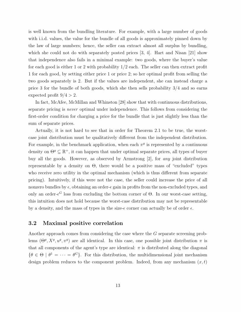
In the comonotonic joint distribution π, there are three possible types, (1, 2), (1, 3),
(2, 4), occurring with probabilities 1/3, 1/6, 1/2 respectively (as shown in Figure 1(a)). If
this is the joint distribution, then we propose the following mechanism: the buyer can
either
• receive good 1 at a price of 1;
• receive good 2 at a price of 3;
• receive both goods at a price of 5; or
14
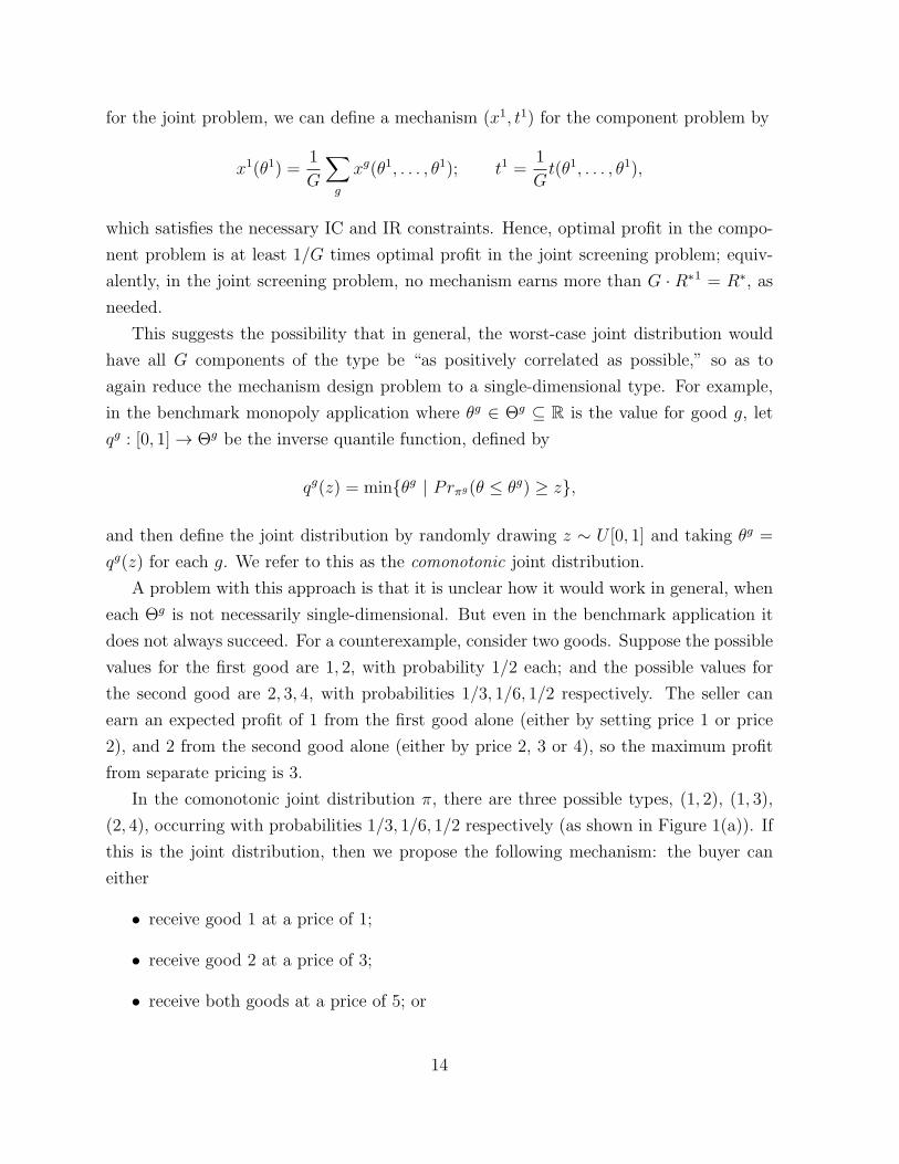
• receive nothing and pay nothing.
Figure 1(b) shows the regions of buyer space in which each option is chosen; in particular,
it is incentive-compatible for the (1, 2)-buyer to buy only good 1, the (1, 3)-buyer to buy
only good 2, and the (2, 4)-buyer to buy the bundle, leading to revenue
1
3· 1 +
1
6· 3 +
1
2· 5 =
10
3> 3.
1/3
1/6
1/2
1 2
2
3
4
θ1
θ2
(a)
(1,0)
1
(0,1)
3
(1,1)
5
θ1
θ2
(b)
1 2
2
3
4
θ1
θ2
3/20
1/10
1/4
7/20
1/15
1/12
(c)
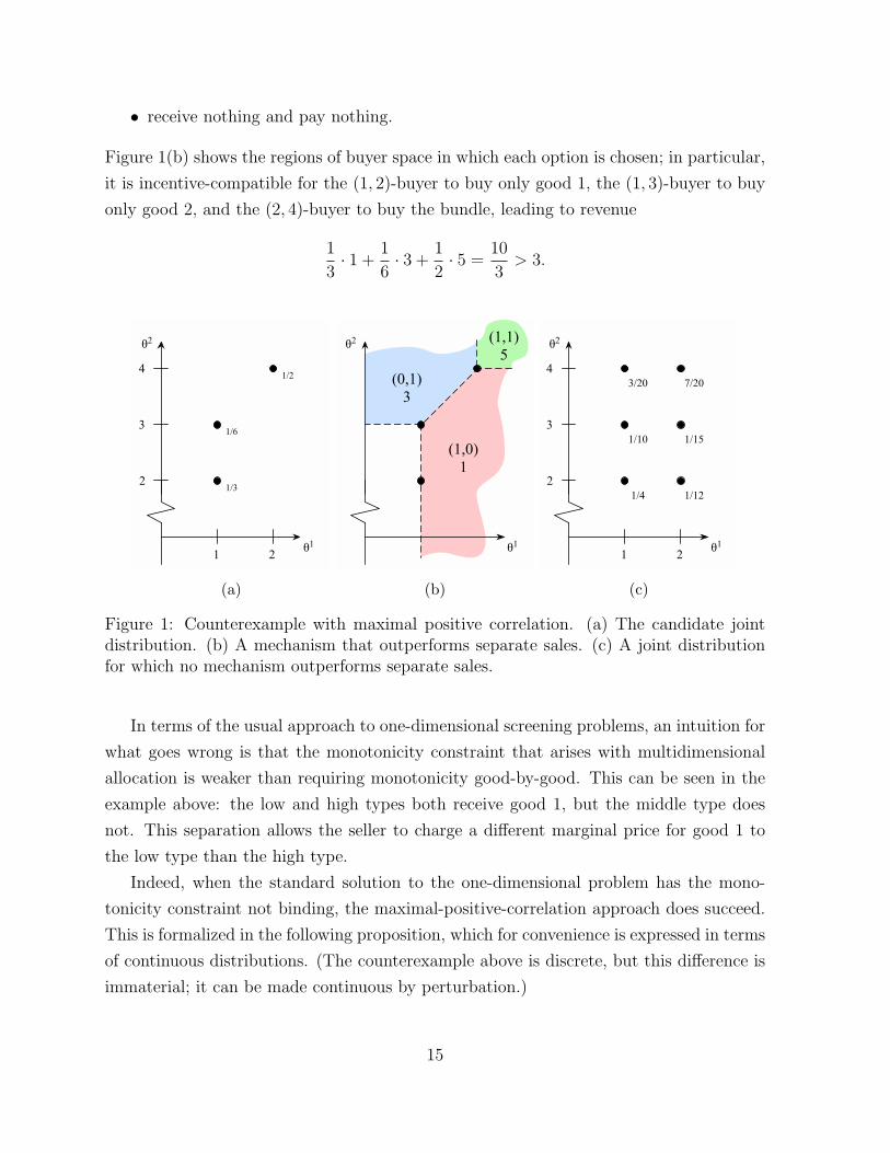
Figure 1: Counterexample with maximal positive correlation. (a) The candidate jointdistribution. (b) A mechanism that outperforms separate sales. (c) A joint distributionfor which no mechanism outperforms separate sales.
In terms of the usual approach to one-dimensional screening problems, an intuition for
what goes wrong is that the monotonicity constraint that arises with multidimensional
allocation is weaker than requiring monotonicity good-by-good. This can be seen in the
example above: the low and high types both receive good 1, but the middle type does
not. This separation allows the seller to charge a different marginal price for good 1 to
the low type than the high type.
Indeed, when the standard solution to the one-dimensional problem has the mono-
tonicity constraint not binding, the maximal-positive-correlation approach does succeed.
This is formalized in the following proposition, which for convenience is expressed in terms
of continuous distributions. (The counterexample above is discrete, but this difference is
immaterial; it can be made continuous by perturbation.)
15
Proposition 3.1. Consider the benchmark monopoly application. Suppose each marginal
distribution πg is represented by a continuous, positive density f g, and write F g for the
cumulative distribution. Suppose that for each g, there is a type θ∗g such that the virtual
value
vg = θg −1− F g(θg)
f g(θg)(3.1)
is negative for θg < θ∗g and positive for θg > θ∗g. Let π be the comonotonic joint
distribution. For this π, no mechanism yields higher expected profit than R∗.
This can be shown by the usual method of ignoring the monotonicity constraint, using
the infinitesimal downward IC constraints to rewrite profit in terms of virtual surplus,
and then maximizing virtual surplus pointwise. The details are in Appendix A.
On the other hand, we can give a partial converse, generalizing the idea of our coun-
terexample to a class of distributions for which monotonicity does bind, so that the
optimal mechanism for one good either sells to some types whose virtual value is negative
or excludes some types whose virtual value is positive:
Proposition 3.2. Consider the benchmark monopoly application with continuous, positive
densities. Let p∗g denote the optimal posted price for each good g, and z∗g = F g(p∗g).
Suppose there are two goods g, g′ for which either
(i) z∗g > z∗g′
but the virtual value vg′
(defined in (3.1)) is negative at θg′
= qg′
(z∗g); or
(ii) z∗g < z∗g′
, but vg′
is positive at θg′
= qg′
(z∗g).
Then, for the comontonic joint distribution π, there exists a mechanism that earns profit
strictly above R∗.
Thus, in the light of Propositions 3.1 and 3.2, our Theorem 2.1 can be seen as a result
about the relationship between multidimensional ironing and single-dimensional ironing.
However, as multidimensional ironing is still poorly understood, we do not pursue this
direction of approach here (besides which, as already indicated, it would not be clear
how to generalize this idea beyond the setting where each component problem is one-
dimensional). Instead, we directly construct our joint distribution π using a duality
approach. For the above example, the π we construct is as shown in Figure 1(c).
In this example, there are other joint distributions that also pin down profit to at most
R∗; all of them place positive probability on at least five of the six possible types. However,
for the distribution shown, a subset of the constraints — namely, the IC constraints for
16
reporting as the next lower value for one good (and truthful reporting for the other good),
plus the IR constraint for the lowest type — are enough to pin down revenue to R∗; and
it is the unique distribution with this property.
Before wrapping up this discussion, we comment that the result of Proposition 3.1
extends more generally to combinations of single-dimensional screening problems with
single-crossing (we omit the details here). This observation lets us elaborate on the rele-
vance of the work by Strausz [39] on deterministic mechanisms, mentioned in Subsection
2.3 above. Strausz shows that in general single-dimensional screening problems where the
monotonicity constraint does not bind in finding the optimal deterministic mechanism,
the optimal probabilistic mechanism is in fact the deterministic one. However, we do not
wish to emphasize these instances here, because these are exactly the cases for which our
comonotonic π succeeds, so Theorem 2.1 is relatively straightforward in these cases.
We turn now to the general proof.
4 The actual proof
The proof is fairly notation-heavy, so it seems helpful to give a more verbal overview first.
The bulk of the proof consists of the case where Θg and Xg and finite; afterwards, we
extend to the general case by an approximation argument.
For the finite case, we regard each component screening problem as a linear program-
ming problem, with the components of the mechanism (the probability of each allocation
at each type, and the payments) as the variables. Then, LP duality tells us that the linear
inequalities that every mechanism (xg, tg) must satisfy — the IC and IR constraints, and
the feasibility constraints (allocation probabilities are nonnegative and sum to one) — can
be multiplied by some weights and added up to give the inequality∑
θg πg(θg)tg(θg) ≤ R∗g.
We would like to find some probability distribution π on Θ so that we can do the same
in the joint screening problem: there should be some weighted sum of the IC, IR, and
feasibility constraints in the joint problem that yields the inequality∑
θ π(θ)t(θ) ≤ R∗.
If we can do this, it shows that no joint screening mechanism can earn expected profit
more than R∗. Our strategy, then, is to simultaneously construct the distribution π and
the multipliers on the constraints so that the constraints add up in the desired way. In
fact, we will need only a subset of the IC constraints — namely, the ones for misreporting
a single component of the type; that is, the IC constraints for type (θg, θ−g) to imitate
a type (θg, θ−g), for some g and θg. Moreover, we will end up using only the constraints
for which the corresponding constraint in the component problem (θg imitating θg) was
17
binding. We are thus studying a relaxed problem, and showing that these constraints
already ensure that no mechanism earns profit above R∗.
Once we have this proof strategy in mind, execution is mostly straightforward (if
involved). The algebra inexorably leads us to formulas that must give us the correct
multipliers, if the strategy is to succeed. We then need to check that these multipliers,
and the corresponding probabilities, are actually nonnegative.
The multipliers we construct for the joint screening problem are (mostly) obtained
by taking the corresponding multipliers from the component problems, and rescaling by
certain reweighting coefficients γg[θ] — one coefficient for each choice of g = 1, . . . , G and
θ ∈ Θ. More specifically, the joint multipliers and probabilities are constructed as follows:
• the multiplier on the IC constraint (θg, θ−g) → (θg, θ−g) equals γg[θg, θ−g] times the
corresponding multiplier on θg → θg in the component problem;
• the multipliers on the feasibility constraints at θ equal γg[θ] times the corresponding
multipliers in the component problems;
• the multiplier on the IR constraint at θ is the product of the corresponding multi-
pliers from the G component problems (no γg used here);
• the probability π(θ) equals γg[θ] · πg(θg), which turns out to be the same for all g.
The γg[θ] need to satisfy a particular system of linear equations; a key step in the
proof is showing that this system actually has a nonnegative solution (Lemma 4.4). Our
proof here is non-explicit, by showing that a linear operator corresponding to the system
has a (nonnegative) fixed point. This ensures that the multipliers and probabilities are
all nonnegative, as required.
We then check that the π constructed above has the correct marginal distributions πg,
and that by multiplying the constraints by these multipliers and summing, we do obtain
the inequality∑
θ π(θ)t(θ) ≤ R∗.
Now it’s time to begin the proof.
4.1 Preliminary tools
We first gather a couple of technical facts about screening problems. For this subsection,
we use the variables (Θ, X, u, π) to refer to an arbitrary screening problem as in Subsection
2.1, not the product environment of our main model.
First, a simple continuity result:
18
Lemma 4.1. Consider a screening environment (Θ, X, u), with Θ, X finite. Then, the
maximum expected profit is continuous as a function of the distribution π.
The straightforward proof is in Appendix A.
A second, related result is an approximation lemma due to Madarasz and Prat [27]
that applies to continuous type spaces. It shows that when each type in a given screening
problem is moved by a small amount, the principal’s optimal profit does not degrade
significantly, even though the optimal mechanism may be discontinuous. The idea is
that any given mechanism can be made robust to slight changes in the type distribution
by refunding a small fraction of the payment to the agent: doing so pads the incentive
constraints in such a way that, if the agent is induced to change his chosen allocation, he
does so in favor of more expensive allocations; and this effect outweighs any small change
in the agent’s location in type space.
Formally, say that two distributions π, π′ ∈ ∆(Θ) are δ-close if Θ can be partitioned
into disjoint measurable sets S1, . . . , Sr such that d(θ, θ′) < δ for any θ, θ′ in the same cell
Sk, and π(Sk) = π′(Sk) for each Sk.
Lemma 4.2. [27] Take the environment (X,Θ, u) as fixed. For any ǫ > 0, there exists
a number δ > 0 with the following property: For any mechanism (x, t), there exists a
mechanism (x, t) such that
(a) for any two types θ, θ′ with d(θ, θ′) < δ, then t(θ′) > t(θ)− ǫ;
(b) for any two distributions π, π′ that are δ-close,
Eπ′ [t(θ)] > Eπ[t(θ)]− ǫ.
Again, we include the proof in Appendix A for completeness.
Finally, we give an elementary algebra lemma that will be useful.
Lemma 4.3. Let c1, . . . , cN , d1, . . . , dN , and r be real numbers, with ci > di ≥ 0 for each
i. Then the system of N linear equations in N real variables,
cixi +∑
j 6=i
djxj = r (i = 1, . . . , N),
has a unique solution, given by
xi =1
ci − di×
r
1 +∑
j
djcj−dj
.
19
Proof. Writing s =∑
j djxj, the system is equivalent to the (N + 1)-variable system
(ci − di)xi + s = r (i = 1, . . . , N); (4.1)∑
j
djxj = s.
The first N equations can be used to write xi = (r − s)/(ci − di), which can be then
plugged into the last equation, which determines s uniquely. Solving for s, then plugging
back into (4.1), gives the stated formula for xi.
4.2 The finite case
Now we start the proof of the theorem. Suppose for now that for each g, both Θg and
Xg are finite. Refer to allocations in Xg simply by numbers 1, 2, . . . , kg. By creating
duplicates if needed, we can assume that each Xg contains the same number of elements,
kg = k. We will also identify a type θg ∈ Θg with the k-dimensional vector specifying its
payoff from each allocation, thus writing θgi instead of ug(i, θg), for i = 1, . . . , k.
We also assume for now that every type has positive probability, πg(θg) > 0. (This is
not quite without loss of generality: note that we cannot simply ignore probability-zero
types, as their IR constraints may affect the set of possible mechanisms. At the end, we
will show how to allow for probability-zero types.)
A mechanism for component g then consists of a vector of |Θg| · (k + 1) numbers,
namely the probabilities of each allocation, xgi (θ
g) for each θg and i = 1, . . . , k, and the
payments tg(θg) for each θg, satisfying the constraints
∑
i
θgi xgi (θ
g)− tg(θg) ≥∑
i
θgi xgi (θ
g)− tg(θg) for all θg, θg ∈ Θg; (4.2)
∑
i
θgi xgi (θ
g)− tg(θg) ≥ 0 for all θg ∈ Θg; (4.3)
xgi (θ
g) ≥ 0 for all θg ∈ Θg, i = 1, . . . , k; (4.4)∑
i
xgi (θ
g) = 1 for all θg ∈ Θg. (4.5)
The maximum expected profit over all such mechanisms is given by
max(xg ,tg)
∑
θg
πg(θg)tg(θg) = R∗g.
20
Maximizing this profit is just a linear programming problem. Hence, by LP duality,
there exist multipliers on the constraints (which are indexed by types, indicated in square
brackets):
λg[θg → θg] ≥ 0 for each θg, θg;
κg[θg] ≥ 0 for each θg;
µgi [θ
g] ≥ 0 for each θg, i;
νg[θg] for each θg
such that adding up λg[θg → θg] times (4.2), κg[θg] times (4.3), µgi [θ
g] times (4.4) and
νg[θg] times (4.5) gives the inequality∑
θg πg(θg)tg(θg) ≤ R∗g.
Writing out these dual constraints explicitly, we have:
∑
θg
λg[θg → θg]θgi −∑
θg
λg[θg → θg]θgi − κg[θg]θgi − µgi [θ
g]− νg[θg] = 0 (4.6)
for each θg and i, as the constraint corresponding to xgi (θ
g);
∑
θg
λg[θg → θg]−∑
θg
λg[θg → θg] + κg[θg] = πg(θg) (4.7)
for each θg, as the constraint corresponding to tg(θg); and from the constants,
−∑
θg
νg[θg] = R∗g. (4.8)
For each component g, we find such multipliers.
Now we look at the joint screening problem. We wish to show that, for some joint
distribution π over Θ, the constraints in the joint screening problem imply that total
profit is at most R∗. This will happen if, analogously to the component problem, we
can find some multipliers on each of the constraints defining the joint problem so that,
when the constraints are suitably multiplied and added up, we end up with the inequality∑
θ π(θ)t(θ) ≤ R∗. Our approach will be to simultaneously construct both the desired
distribution π and the multipliers.
As outlined earlier, we shall not use all of the constraints in the joint screening problem.
In particular, we use only the incentive constraints for an agent to misrepresent one
component of his type. Thus, we write a mechanism in the joint problem as a vector of
21
|Θ| · (kG+ 1) numbers, xgi (θ) for each θ, g, and i, and t(θ) for each θ; and these numbers
must satisfy the following constraints (among others):
∑
g
∑
i
θgi xgi (θ
h, θ−h)− t(θh, θ−h) ≥∑
g
∑
i
θgi xgi (θ
h, θ−h)− t(θh, θ−h) (4.9)
for each h, θh, θh, θ−h;∑
g
∑
i
θgi xgi (θ)− t(θ) ≥ 0 for all θ ∈ Θ; (4.10)
xgi (θ) ≥ 0 for all θ, g, i; (4.11)
∑
i
xgi (θ) = 1 for all θ, g. (4.12)
We begin to specify our desired multipliers. We first define κ[θ], for each θ ∈ Θ, by
κ[θ] =∏
g
κg[θg].
Note for future reference that, for each fixed g, if we sum up (4.7) over all θg, the λg[· · · ]
terms cancel, and we are left with
∑
θg
κg[θg] =∑
θg
πg(θg) = 1. (4.13)
Multiplying across all g, we then get
∑
θ∈Θ
κ[θ] = 1 (4.14)
as well. And if we fix g and θg, and multiply (4.13) only for all other components h 6= g,
we likewise get ∑
θ−g∈Θ−g
κ[θg, θ−g] = κg[θg] (4.15)
which will also be useful later.
Now, the key step in constructing our remaining multipliers is to show that a particular
system of equations has a nonnegative solution:
Lemma 4.4. There exist nonnegative numbers γg[θ], for each θ ∈ Θ and each g, satisfying
22
the equations
γg[θ]×
∑
θg
λg[θg → θg] + κg[θg]
+
∑
h 6=g
γh[θ]×
∑
θh
λh[θh → θh]
=∑
h
∑
θh
γh[θh, θ−h]λh[θh → θh] + κ[θ] (4.16)
for all θ and all g.
(The right-side sum over h includes h = g as well as h 6= g.)
Proof. First, for any fixed vector γ of |Θ| ·G real numbers γg(θ), consider seeking a vector
β consisting of |Θ| ·G numbers βg(θ) to satisfy the |Θ| ·G linear equations
βg[θ]×
∑
θg
λg[θg → θg] + κg[θg]
+
∑
h 6=g
βh[θ]×
∑
θh
λh[θh → θh]
=∑
h
∑
θh
γh[θh, θ−h]λh[θh → θh] + κ[θ] (4.17)
for each θ and g. Note that this system breaks into |Θ| smaller systems: for each fixed θ,
we have a system of G equations in the G variables βg[θ] (g = 1, . . . , G). Moreover, this
smaller system satisfies the conditions of Lemma 4.3, since
∑
θg
λg[θg → θg] + κg[θg]
−
∑
θg
λg[θg → θg]
= πg(θg) > 0 (4.18)
by (4.7). Therefore, we obtain a unique vector β satisfying these equations, with formula
given by Lemma 4.3. Moreover, the components of β depend linearly on γ, and β is
nonnegative if γ is.
Then, define B(γ) to be the resulting vector β. This defines a linear map B (more
precisely, an affine map) from R|Θ|·G to itself. We would like to show that B has a fixed
point, with nonnegative components.
Define S : R|Θ|·G → R by
S(γ) =∑
θ
∑
g
γg[θ]×
∑
θg
λg[θg → θg]
.
23
This is a linear function with all nonnegative coefficients. Then, if γ ∈ R|Θ|·G is nonnega-
tive, the formula from Lemma 4.3 implies
S(B(γ)) =∑
θ
τ [θ]
1 + τ [θ]
∑
h
∑
θh
γh[θh, θ−h]λh[θh → θh] + κ[θ]
where
τ [θ] =∑
g
∑θgλg[θg → θg]
πg(θg).
(We have used (4.18) to simplify the denominator.) In particular, taking ρ = maxθτ [θ]
1+τ [θ]<
1, we have (by nonnegativity)
S(B(γ)) ≤ ρ ·∑
θ
∑
h
∑
θh
γh[θh, θ−h]λh[θh → θh] + κ[θ]
= ρ · (S(γ) +
∑
θ
κ[θ]).
Hence, recalling∑
θ κ[θ] = 1 from (4.14), if S(γ) ≤ ρ/(1− ρ), then
S(B(γ)) ≤ ρ · (S(γ) + 1) ≤ ρ
(ρ
1− ρ+ 1
)=
ρ
1− ρ.
Thus, the affine map B maps the set of nonnegative vectors γ satisfying S(γ) ≤
ρ/(1− ρ) into itself.
We would now like to apply a fixed-point theorem. However, the above set is not
necessarily compact, since some coefficients of S may be zero. To rectify this, define a
pair (θ, g) to be active if λg[θg → θg] > 0 for at least one value of θg. Notice that the
value of B(γ) depends only on the coordinates of γ that correspond to active pairs, since
the inactive coordinates contribute nothing to the right side of (4.17). Thus, if we let
Z ⊆ Θ×{1, . . . , G} be the set of active pairs, B induces a linear map B : R|Z| → R|Z|, by
taking any γ consistent with the given active coordinates, applying B, and disregarding
the inactive coordinates of the output. Likewise, the value of S(γ) depends only on the
active coordinates of γ, and the coefficient of each such coordinate is strictly positive, by
definition of active pairs. Hence, S induces a strictly increasing linear map S : R|Z| → R.
Then, B maps the set of nonnegative |Z|-dimensional vectors γ satisfying S(γ) ≤
ρ/(1 − ρ) into itself; and this set is compact. Therefore, by (say) Brouwer’s theorem, B
has a fixed point γ in this set. By lifting this γ to an element of R|Θ|·G and applying B, we
get a fixed point of B, with all nonnegative coordinates. This satisfies (4.16), as needed.
24
Now, taking the γg[θ] as given by the lemma, we are ready to construct the rest of our
multipliers, and our joint distribution. We do the latter first. For each θ and g, subtract∑
h γh[θ]×
(∑θhλh[θh → θh]
)from both sides of (4.16), and apply (4.7); we then have
γg[θ]πg(θg) = −∑
h
∑
θh
γh[θ]λh[θh → θh] +∑
h
∑
θh
γh[θh, θ−h]λh[θh → θh] + κ[θ]. (4.19)
The right hand side depends only on θ and not on g. In particular, we can define π(θ) to
be equal to this expression, and we have π(θ) = γg[θ]πg(θg) for each g.
This gives us a nonnegative number π(θ) for each θ. Our next task is to check that
these form a joint distribution, and that it has the correct marginals πg. Note that for
this it suffices to show the following:
Lemma 4.5. For each g and each value of θg,∑
θ−g γg[θg, θ−g] = 1.
Proof. Fix any g. Consider the following system of |Θg| linear equations in |Θg| variables,
one variable zg[θg] for each θg:
zg[θg]×
∑
θg
λg[θg → θg] + κg[θg]
=
∑
θg
zg[θg]× λg[θg → θg] + κg[θg] (4.20)
for each θg.
Note that the system has the trivial solution zg[θg] = 1 for all θg. On the other hand,
taking zg[θg] =∑
θ−g γg[θg, θ−g] also gives a solution. To see this, hold fixed θg, vary θ−g,
and sum up the resulting copies of equation (4.16). For each h 6= g, the terms in the
second sum on the left side of (4.16) cancel with the terms in the first sum on the right
side — the term γh[θg, θh, θ−gh]λh[θh → θh] appears once on each side for each choice of
θh, θh and θ−gh. After cancelling these terms we are left with
∑
θ−g
γg[θg, θ−g]×
∑
θg
λg[θg → θg] + κg[θg]
=
∑
θ−g
∑
θg
γg[θg, θ−g]λg[θg → θg]+∑
θ−g
κ[θg, θ−g].
Applying (4.15) to reduce the last right-hand sum to κg[θg], we confirm that zg[θg] =∑
θ−g γg[θg, θ−g] is a solution to (4.20).
However, the inequality (4.18) implies that the matrix corresponding to this linear
system is strictly diagonally dominant, and therefore invertible (see e.g. [31, p. 226] or
25
[24, p. 302]). Therefore, the system of equations can have only one solution. It follows
that∑
θ−g γg[θg, θ−g] = 1 for each θg, as claimed.
This verifies that π is indeed a joint distribution with the correct marginals πg.
We now define the remaining multipliers for the joint mechanism design problem. For
each g, put
λg[(θg, θ−g) → (θg, θ−g)] = γg[θg, θ−g]× λg[θg → θg] for each θg, θg, θ−g;
µgi [θ
g, θ−g] = γg[θg, θ−g]× µgi [θ
g] for each θg, θ−g, i;
νg[θg, θ−g] = γg[θg, θ−g]× νg[θg] for each θg, θ−g.
This is slightly overloaded notation since we used the same letters λg[· · · ], µgi [· · · ], ν
g[· · · ]
for multipliers in the component problem. Note however that we are distinguishing the
multipliers in the joint screening problem by using joint-screening types for the bracketed
indices, so no genuine ambiguity arises. Because all the γg[· · · ] are nonnegative, the newly
defined multipliers λg[· · · ] and µgi [· · · ] are also nonnegative.
Now consider any possible mechanism (x, t) for the joint screening problem. It satisfies
the constraints (4.9–4.12).
For each h, θh, θh and θ−h, multiply (4.9) by λh[(θh, θ−h) → (θh, θ−h)]; for each θ,
multiply (4.10) by κ[θ]; for each θ, g, i, multiply (4.11) by µgi [θ]; and for each θ, g, multiply
(4.12) by νg[θ]; and sum up. What do we get?
To avoid ambiguity with signs, let us move all terms to the right-hand side of the
summed-up inequality. Then, we successively determine the coefficient of each variable
xgi (θ), the coefficient of t(θ), and the constant term.
First, consider the coefficient of xgi (θ), for each θ, g, and i. This variable occurs on the
left side of (4.9) once for each choice of h and each θh; in each such instance, it appears
with coefficient λh[(θh, θ−h) → (θh, θ−h)]θgi . It also occurs an equal number of times on
the right side of (4.9), once for each possible h and θh, corresponding to the IC constraint
(θh, θ−h) → (θh, θ−h); in this case, the resulting coefficient is λh[(θh, θ−h) → (θh, θ−h)]θgi if
h 6= g, and is λh[(θh, θ−h) → (θh, θ−h)]θgi if h = g. This variable also occurs once on the
left side of (4.10), with coefficient κ[θ]θgi ; once on the left side of (4.11), with coefficient
µgi [θ]; and once on the left side of (4.12), with coefficient νg[θ]. Adding up, then, the
26

difference between the right- and left-side coefficients of xgi (θ) is
∑
h 6=g
∑
θh
λh[(θh, θ−h) → (θh, θ−h)]θgi +∑
θg
λg[(θg, θ−g) → (θg, θ−g)]θgi
−∑
h
∑
θh
λh[(θh, θ−h) → (θh, θ−h)]θgi − κ[θ]θgi − µgi [θ]− νg[θ].
Plugging in explicitly from the definitions of our multipliers, this becomes
∑
h 6=g
∑
θh
γh[θ]λh[θh → θh]θgi +∑
θg
γg[θ]λg[θg → θg]θgi (4.21)
−∑
h
∑
θh
γh[θh, θ−h]λh[θh → θh]θgi − κ[θ]θgi − γg[θ]µgi [θ
g]− γg[θ]νg[θg].
The first, third and fourth terms, together, are equal to θgi times the quantity
∑
h 6=g
∑
θh
γh[θ]λh[θh → θh]−∑
h
∑
θh
γh[θh, θ−h]λh[θh → θh]− κ[θ]
and this latter quantity, by (4.16), is equal to
−γg[θ]×
∑
θg
λg[θg → θg] + κg[θg]
.
Thus, (4.21) simplifies to
∑
θg
γg[θ]λg[θg → θg]θgi − γg[θ]
∑
θg
λg[θg → θg] + κg[θg]
θgi − γg[θ]µg
i [θg]− γg[θ]νg[θg].
We can pull out a factor of γg[θ] and the rest is equal to
∑
θg
λg[θg → θg]θgi −
∑
θg
λg[θg → θg] + κg[θg]
θgi − µg
i [θg]− νg[θg].
This is exactly zero, by (4.6). Thus, in our summed-up inequality, all xgi (θ) terms cancel
out completely.
Next, we consider the coefficient of t(θ), for each θ. This appears on the left side of
(4.9) with coefficient −λh[(θh, θ−h) → (θh, θ−h)], for each h and θh, and on the right side
27
of (4.9) with coefficient −λh[(θh, θ−h) → (θh, θ−h)], for each h and θh; it also appears on
the left side of (4.10) once, with coefficient −κ[θ]. Thus, when we sum up, the difference
in the coefficients of t(θ) between the right and left sides is
−∑
h
∑
θh
λh[(θh, θ−h) → (θh, θ−h)] +∑
h
∑
θh
λh[(θh, θ−h) → (θh, θ−h)] + κ[θ]
which, by definition of the joint λh multipliers, equals
−∑
h
∑
θh
γh[θ]λh[θh → θh] +∑
h
∑
θh
γh[θh, θ−h]λh[θh → θh] + κ[θ].
This is equal to π(θ), by definition of π (4.19).
Finally, we consider the constant terms. The only nonzero constants arise from (4.12),
which gives νg[θ] on the right side for each θ and g; summing then gives
∑
g
∑
θ
νg[θ] =∑
g
∑
θ
γg[θ]νg[θg]
=∑
g
∑
θg
(∑
θ−g
γg[θg, θ−g]
)νg[θg]
=∑
g
∑
θg
νg[θg] (by Lemma 4.5)
=∑
g
(−R∗g) (by (4.8))
= −R∗.
In conclusion, our grand added-up inequality reads simply
0 ≥∑
θ
π(θ)t(θ)−R∗.
So any joint screening mechanism gives expected profit at most R∗ with respect to the
type distribution π, which is what we wanted to show.
This covers the case where each πg has full support. To allow for probability-zero
types, we use our earlier continuity result, Lemma 4.1.
For each g, suppose πg is an arbitrary distribution on Θg, with R∗g the corresponding
maximum expected profit. Let πg1 , π
g2 , . . . be a sequence of full-support distributions on
Θg that converges to πg. Then, if we let R∗g1, R
∗g2, . . . be the corresponding values of the
28
maximum expected profit, Lemma 4.1 says that R∗gn → R∗g as n → ∞.
For each n, the proof we have just completed shows that there exists a joint distribution
πn on Θ, with marginals πgn, such that no mechanism earns an expected profit of more than
R∗n =
∑g R
∗gn with respect to πn. By compactness, we can assume (taking a subsequence
if necessary) that πn converges to some distribution π on Θ. Then π has marginal πg
on each Θg. And for any mechanism (x′, t′), we have Eπn[t′(θ)] ≤ R∗
n; taking limits as
n → ∞, we have Eπ[t′(θ)] ≤ R∗. Thus, no mechanism earns expected profit more than
R∗ on distribution π.
4.3 The general case
Now we can give the general proof of Theorem 2.1, with potentially infinite type and
allocation spaces.
First, extending to general allocation spaces, but keeping type spaces finite, is com-
pletely straightforward. Indeed, suppose each Θg is finite, and let R∗g be the optimal
revenue in component g, and R∗ =∑
g R∗g. Suppose there exists a mechanism (x′, t′)
that achieves revenue at least R∗+ ǫ with respect to every joint distribution π ∈ Π, where
ǫ > 0.
For each component g, define an auxiliary screening problem (Θg, Xg, ug, πg) as follows:
Θg = Θg and πg = πg; Xg = {x′g(θ) | θ ∈ Θ}; ug(xg, θg) = Eug(xg, θg). That is, we
consider only the component-g allocations which were actually assigned to some type in
the mechanism (x′, t′); such an allocation may have been a lottery, but we treat it as a
single allocation in the new screening problem. It is evident that any mechanism for this
new screening problem translates to a mechanism for the original component-g screening
problem, with the same expected profit; hence, the optimal profit for the new component-
g screening problem is R∗g ≤ R∗g. Because Θg and Xg are finite, we can apply the case
of the previous subsection to see that there is a joint distribution π for which no joint
screening mechanism can give expected profit more than R∗. But (x′, t′) evidently gives us
a joint screening mechanism for the new problem, which produces expected profit ≥ R∗+ǫ
for every possible joint distribution — a contradiction.
Finally, we can remove the restriction to finite type spaces. Here is where we will apply
Lemma 4.2, the approximation result for continuous types. Consider the general setting
of Subsection 2.2. Let R∗ be defined as in that section, and suppose, for contradiction,
that there exists a mechanism (x′, t′) that achieves profit at least R∗ + ǫ against every
possible joint distribution π, where ǫ > 0.
29
For each component g, let δg be as given by Lemma 4.2 with ǫ/(2G+1) as the allowable
profit loss. By making δg smaller if necessary, we may also assume that any two types
at distance at most δg have their utility for every xg ∈ Xg differ by at most ǫ/(2G + 1).
Also, consider the joint screening environment, with the metric on Θ given by the sum of
componentwise distances, and let δ be as given by Lemma 4.2 with ǫ/(2G+1) as allowable
loss again. Now let δ = min{δ1, . . . , δG, δ/G}.
For each g, we form an approximate distribution on Θg with finite support, as follows:
Let Θg be a finite subset of Θg, with the property that every element of Θg is within
distance δ of some element of Θg (this can be done by compactness). Arbitrarily partition
Θg into disjoint measurable subsets Sgθg , for θ
g ∈ Θg, such that each element of any Sgθg
is within distance δ of θg, and θg itself is in Sgθg . Then define a distribution πg ∈ ∆(Θg),
supported on Θg, by πg(θg) = πg(Sgθg).
Evidently, πg is δ-close to πg. Therefore, the maximum profit attainable in the screen-
ing problem (Θg, Xg, ug, πg) is at most R∗g + ǫ/(2G+1): otherwise, Lemma 4.2 would be
violated in going from πg from πg.
In turn, we can view πg as a distribution just on Θg, and any mechanism for screen-
ing problem (Θg, Xg, ug, πg) extended to a mechanism on the whole type space Θg, by
assigning each type its preferred outcome from the set {(xg(θg), tg(θg)) | θg ∈ Θg}, and
subtracting ǫ/(2G+ 1) from all payments (in order to make sure that IR is still satisfied
for types outside of Θg). This extension causes a profit loss of ǫ/(2G + 1). We con-
clude that the maximum profit attainable in screening problem (Θg, Xg, ug, πg) is at most
R∗g + 2ǫ/(2G+ 1).
Since this is true for each g, we can apply the finite-type-space version of our result
to conclude the following: there is a distribution π on Θ = ×g Θg, with marginals πg, for
which any mechanism earns expected profit at most R∗ + 2Gǫ/(2G+ 1).
Now we will construct a measure on Θ based on our discretization, but with marginals
given by the original πg. For each θ = (θ1, . . . , θG) ∈ Θ, let Sθ ⊆ Θ be the product set
×g Sgθg ; notice that as θ varies over Θ, the sets Sθ form a partition of Θ.
For each such θ, we define a measure πθ on Sθ as follows. If πg(θg) = 0 for some g, let
πθ be the zero measure. Otherwise, consider the conditional probability measure πg|Sgθg
for each component g (which is well-defined since πg assigns positive probability to Sgθg).
Define πθ to be the product of these conditional measures, multiplied by the scalar π(θ).
We can extend πθ to a measure on all of Θ (by taking it to be zero outside Sθ). Now
simply define a measure π on Θ as the sum of πθ, over all θ ∈ Θ.
Note that π is indeed a probability measure; this follows from the fact that the measure
30
assigned to any Sθ equals π(θ), and hence the total measure of Θ is
π(Θ) =∑
θ∈Θ
π(Sθ) =∑
θ∈Θ
π(θ) = 1.
In fact, its marginal along component g must equal πg, for each g. This follows from two
facts: first, the probability assigned to any cell Sgθg under this marginal is equal to
∑
θ−g∈Θ−g
π(S(θg ,θ−g)) =∑
θ−g∈Θ−g
π(θg, θ−g) = πg(θg) = πg(Sgθg);
and second, conditional on cell Sgθg , the distribution along the g-component follows πg|Sg
θg
(because this is true for each of the cells S(θg ,θ−g)).
Consequently, our mechanism (x′, t′) satisfies Eπ[t′(θ)] ≥ R∗ + ǫ, by assumption.
In addition, the fact that π(Sθ) = π(θ) for every θ ∈ Θ implies that π is δ-close to
π, since every element of Sgθg is within distance δ ≤ δ/G of θg, for each component g.
Consequently, Lemma 4.2 assures us the existence of a mechanism whose expected profit
with respect to π is greater than (R∗ + ǫ)− ǫ/(2G+ 1) = R∗ + 2Gǫ/(2G+ 1).
But we already showed it is impossible to earn profit greater than R∗ + 2Gǫ/(2G+ 1)
against π. Contradiction.
�
5 Sensitivity analysis
A natural response to Theorem 2.1 is to ask how sensitive the result is to the assumption
of extreme uncertainty about the joint distribution π. In particular, our proof approach
constructs a very specific π — and not one that has an immediate intuitive meaning
(unlike, say the independent distribution, or the maximal-correlation distribution from
Subsection 3.2). If there were some other mechanism that performed better than sepa-
rate screening as long as the joint distribution is not this specific π, that would lessen
the appeal of the result — both its methodological appeal (since it could be taken to say
that our approach of taking the worst case over Π is somewhat contrived), and its literal
appeal as an explanation of, say, separate posted prices in the real world. Accordingly,
this section will briefly attempt to investigate how often the result that separate screening
is optimal becomes overturned if the designer has a little information about the joint dis-
tribution. For concreteness, we focus on the benchmark monopoly application throughout
31
this section.
One immediate difficulty is that it is not clear exactly what it means to have “a little
information” about π. One might impose some one-dimensional moment restriction, of
the form
Eπ[z(θ)] = 0 (5.1)
or
Eπ[z(θ)] ≥ 0 (5.2)
for some function z : Θ → R, and let Π′ be the set of all π ∈ Π satisfying the restriction,
and then evaluate a mechanism (x, t) according to infπ∈Π′ Eπ[t(θ)] instead of the original
objective (2.3), and ask whether separate sales is still optimal. However, it is clear that
some versions of this approach will give a negative result. For example, we know that
some other mechanisms (x′, t′) will sometimes give higher profit than R∗, so if our moment
restriction is of the form Eπ[t′(θ)] ≥ R′ for R′ > R∗, clearly our result fails. The question
then seems to be, what are the interesting restrictions to consider?
We explore two approaches here. First, we consider one particular moment restriction
suggested by the literature, namely negative correlation in values between two goods.
Second, we show that in the finite-type version of the model, in general there is an open
set of distributions π for which separate pricing is optimal; this gives some assurance
that Theorem 2.1 is not a knife-edge result, without needing to take a stand on specific
moment restrictions.
5.1 Negative correlation
One of the main intuitions from the early bundling literature is that bundling is profitable
when values for goods are negatively correlated, although the argument comes largely from
examples [38, 1]; in the extreme case where the total value for all goods is deterministic,
the seller can extract the full surplus by selling the bundle of all goods. In addition, this
seems a natural place to look for restrictions to overturn the separation result, since it in
a sense opposite to the positively-correlated case of Subsection 3.2.
Accordingly, let us take the restriction of negative correlation literally, and test it by
considering G = 2 goods and imposing the moment restriction
Eπ[θ1θ2] ≤ Eπ1 [θ1]× Eπ2 [θ2]
on the possible joint distributions π. It turns out that with this restriction, it may or may
32

not happen that the worst-case-optimal revenue is still the R∗ from selling separately.
To get some sense of whether one case or the other is common, random numerical
experiments were run in Matlab, using finite type spaces Θ. Note that for any one-
dimensional moment restriction of the form Eπ[z(θ)] ≥ 0, the worst-case-optimization
problem
max(x,t)∈M
(minπ∈Π′
Eπ[t(θ)]
)(5.3)
can be computationally implemented as follows: Since the inner minimization is a linear
program (with the probabilities π(θ) as the choice variables), by LP duality, it can also
be expressed as a maximization problem, namely
maxαg [θg ],β
∑
g
∑
θg
αg[θg]
over all choices of real numbers αg[θg] (for each g = 1, . . . , G and θg ∈ Θg) and β ≥ 0
satisfying ∑
g
αg[θg] + βz(θ) ≤ t(θ) for all θ = (θ1, . . . , θG) ∈ Θ. (5.4)
Therefore, the problem in (5.3) can be expressed as a single maximization — over all
choices of the mechanism (x, t), and all αg[θg] and β satisfying (5.4) — that can be solved
as a standard LP.
In the simulations, we randomly generated 1000 choices for the marginal distributions
(π1, π2), calculated the mechanism that maximizes the worst-case revenue over negatively
correlated distributions as just described, and checked whether the worst-case revenue
was strictly higher than obtained by selling the two goods separately. The set of possible
values for each good was Θ1 = Θ2 = {1, 2, 3, 4, 5}, and the marginals πg were generated
by drawing a probability uniformly from [0, 1] for each value, then rescaling to make the
probabilities sum to 1.
The result was that in 970 of the 1000 trials, the worst-case revenue was still the R∗
from selling separately.1
One might protest that this sensitivity test is too weak, because it is inappropriate
to take negative correlation so literally; it is no surprise that one misspecified inequality
restriction often fails to rule out some worst-case distributions. It is not clear what
1In 35 trials, Matlab’s LP solver failed to converge due to numerical error. So a more certain lowerbound is that the result held in at least 93.5% of trials. (The simulations were done in Matlab R2014bon an iMac running OS X 10.8.5.)
33
an appropriate sharper test would be, but one possible test would be to impose negative
affiliation on π — that is, negative correlation conditional on θ ∈ Θ1×Θ2, for all nonempty
subsets Θ1 ⊆ Θ1, Θ2 ⊆ Θ2. This limits the possible π to a much smaller set, so one would
expect separate sales to be worst-case optimal much less often.
It is not immediately clear how to repeat the above computational exercise with the
restriction of negative affiliation, since it is not a linear constraint on π, so the worst-case
optimization cannot readily be expressed as a linear program. However, if we move to the
continuous-type setting, we can obtain a negative result: separate sales is (essentially)
always dominated by bundling. The dominance is weak for a given bundle price, but can
be made strict by randomizing the bundle price.
Proposition 5.1. Consider the benchmark monopoly application, with G = 2. Suppose
each set of values Θg is an interval in R++, and each marginal distribution πg is repre-
sented by a continuous, positive density f g. Assume that for each g, the optimal separate
price p∗g is strictly in the interior of Θg. Then there exist ǫ, ǫ > 0, q ∈ (0, 1), and R′ > R∗
such that the following hold:
(a) The mechanism that offers each good g with price p∗g or the bundle of both goods at
price p∗1 + p∗2 − ǫ earns expected profit at least R∗ for any negatively affiliated joint
distribution π ∈ Π.
(b) Consider the following mechanism: first randomly choose ǫ = ǫ with probability q or
ǫ = ǫ with probability q = 1− q; then offer each good g with price p∗g, or the bundle
of both goods at price p∗1 + p∗2 − ǫ. This mechanism earns expected profit at least
R′, for any negatively affiliated joint distribution π ∈ Π.
The argument is a straightforward extension of that given by McAfee, McMillan, and
Whinston [28] for the independent case, obtained by looking at the first-order condition
for ǫ. The proof is in Appendix A.
5.2 Open sets of distributions
Another approach to sensitivity analysis, which avoids making any particular choices of
moment restrictions, is to look at the set of distributions π for which separate pricing
is optimal, and ask how small this set is. If it contained only the specific distribution
constructed in Section 4, then our result would indeed be a knife-edge result. However,
we will show here that the situation is not so extreme: in particular, when the type space
is finite, the set of such worst-case π is an open set (in the natural topology on Π).
34
We could also simply try to show that there is an open set of possible moment re-
strictions z in (5.1) for which the worst-case optimal revenue is R∗. Note however that
this is a much weaker statement than existence of an open set of π’s as above. In fact,
as long as there is more than one π — say π1 and π2 — for which optimal revenue is R∗,
then for any z in the open set satisfying Eπ1[z(θ)] < 0 and Eπ2
[z(θ)] > 0, there is some
convex combination of π1 and π2 for which E[z(θ)] = 0, and so the worst-case objective
(5.3) equals R∗.
The important step is the following.
Lemma 5.2. Consider the benchmark monopoly application. Suppose each set of values
Θg is finite, that each πg has full support, and also suppose that for each single-good
problem πg, the optimal price is unique. Then, there exists a joint distribution π ∈ Π for
which selling each good separately constitutes the unique optimal mechanism.
The proof builds on the construction in Section 4 by analyzing the binding incentive
constraints. The proof is fairly involved, so we leave it to Appendix A.
Now we infer the non-knife-edge result:
Corollary 5.3. In the setting of Lemma 5.2, there exists a set of joint distributions
Π ⊆ Π, which is open (in the relative topology on Π, as a subset of R|Θ|), and such that
for any π ∈ Π, no joint screening mechanism earns an expected profit higher than R∗.
Proof. As argued in the proof of Lemma 4.2 in the appendix, when looking for optimal
mechanisms, we can restrict to ones whose payments are all in [−t, t] for some sufficiently
high constant t. Then, the effective space of mechanisms M′ becomes a convex polytope,
since it is a compact set of |Θ| · (G + 1)-dimensional vectors defined by certain linear
constraints. Therefore, it is the convex hull of its vertices (see e.g. [41, Theorem 1.1]), i.e.
there exist some mechanisms M1, . . . ,MK such that every mechanism in M′ equals some
convex combination of them.
By Lemma 5.2, there exists some particular π∗ ∈ Π for which the separate-sales mech-
anism earns strictly higher expected profit than any other mechanism. Since expected
profit is a linear function on M′, it is maximized at one of the corners, so the separate-
sales mechanism must be one of these corners, say M1. By continuity, for any sufficiently
nearby π, M1 still gives strictly higher expected profit than M2, . . . ,MK , and so strictly
higher than any convex combination, i.e. no mechanism attains higher profit than R∗.
35

We note that this result does not extend to the continuous-type case. If, for example,
each Θg is an interval in R+, with a unique optimal price p∗g that is in the interior, then
for any joint distribution such that the optimal profit is R∗, it can be perturbed by an
arbitrarily small amount so that offering the bundle of goods 1 and 2 at a price p∗1+p∗2−ǫ
(in addition to offering each good g separately at price p∗g) earns strictly higher profit for
small ǫ. As in [28], this can be seen by looking at the first-order condition with respect
to ǫ. We omit the details.
However, we do still have an open set of moment restrictions z for which the worst-
case optimum remains R∗, as long as there is more than one joint distribution π that pins
profit down to R∗ (which will be true in general).
6 Concluding comments
Since this paper has focused on a single main result, there is hardly a need to use this
space to reorganize and summarize the contribution. Instead, we conclude by briefly
discussing some aspirations for future work. As described in the introduction, the main
purpose of this paper has been to advance a possible new modeling approach to attack
multidimensional screening problems, where the traditional approach has often given in-
tractable models. Our result here is certainly only a step in this direction. In particular,
there are two natural goals for further work that, if they could be attained, would (in this
author’s view) constitute a more persuasive case for the promise of this approach:
• First, to have a simpler and more intuitive proof of Theorem 2.1, ideally follow-
ing the reasoning sketched in the introduction — that the profit from screening
separately on each component g is known independently of the joint distribution,
whereas any mechanism in which the components interact seems sensitive to the
joint distribution.
• Second, to have fruitful applications of the method to new economic questions.
More specifically, this would mean identifying some applied-theory question involv-
ing multidimensional screening, where a traditional model would be intractable, and
applying the robust approach to write down a model that can be solved, leading
to new insights. As noted before, the important general insights in multidimen-
sional screening are likely to arise when there are systematic interactions between
the different dimensions, which is exactly what the model in this paper has ruled
36
out. However, this paper may provide a useful starting point by showing how to
first eliminate interactions other than the one to be examined.
Earlier work by this author gave a similar application of the method in a moral haz-
ard setting, taking a simple robust approach to principal-agent contracting [12] and
applying it to gain traction on the more complex problem of incentivizing informa-
tion acquisition [11]. Whether similar progress can be made in a multidimensional
screening context remains to be seen.
In addition, there are some more technical directions in which one might try to extend
Theorem 2.1. For example, a natural question is whether some version of the result holds
with multiple agents. Suppose, say, there are G goods to be auctioned to n buyers, and
the seller knows the marginal distribution of each buyer’s value for each good g, and knows
that the values for any given good g are independent across buyers, but does not otherwise
know how the Gn values are jointly distributed. Is it true that the worst-case revenue-
maximizing mechanism for selling all G goods is simply to sell each good separately, using
the optimal auction [30] for that good?
A Omitted proofs
Proof of Proposition 3.1. For notational convenience, let us parameterize types directly
by z, and write θg(z) for the corresponding value for good g. Thus, for any mechanism
(x, t), x(z) ∈ [0, 1]G indicates type z’s probability of receiving each good, and t(z) ∈ R
indicates z’s payment; incentive-compatibility (2.1) becomes
∑
g
θg(z)xg(z)− t(z) ≥∑
g
θg(z)xg(z)− t(z) for all z, z ∈ [0, 1], (A.1)
and individual rationality (2.2) becomes
∑
g
θgxg(z)− t(z) ≥ 0. (A.2)
The claim is that for any such mechanism, expected revenue satisfies
∫ 1
0
t(z) dx ≤ R∗.
Following the standard method, let U(z) =∑
g θg(z)xg(z)− t(z) denote the payoff of
37
type z. So for z′ ≥ z, (A.1) gives
U(z′) ≥ U(z) +∑
g
(θg(z′)− θg(z))xg(z) ≥ U(z). (A.3)
Thus, U is weakly increasing, hence differentiable almost everywhere, and equal to the
integral of its derivative. Moreover, at each point of differentiability, the envelope theorem
applied to (A.3) gives us
dU
dz=∑
g
dθg(z)
dzxg(z) =
∑
g
1
f g(θg(z))xg(z).
Therefore,
U(z) = U(0) +
∫ z
0
dU(z)
dzdz = U(0) +
∑
g
∫ z
0
xg(z)
f g(θg(z))dz.
Consequently, profit is
∫ 1
0
t(z) dz =
∫ 1
0
(∑
g
θg(z)xg(z)− U(z)
)dz
=
∫ 1
0
(∑
g
θg(z)xg − U(0)−∑
g
∫ z
0
xg(z)
f g(θg(z))dz
)dz
≤∑
g
[∫ 1
0
θg(z)xg(z) dz −
∫ 1
0
(∫ z
0
xg(z)
f g(θg(z))dz
)dz
]
where the last inequality holds because U(0) ≥ 0 by (A.2). Switching the variables in the
second integral and changing the order of integration gives
=∑
g
[∫ 1
0
(θg(z)−
1− z
f g(θg(z))
)xg(z) dz
]. (A.4)
Now, for each g, we can see that the expression in parentheses is exactly the virtual value
vg corresponding to marginal type θg(z). Hence, by assumption, this quantity is negative
for θg(z) < θ∗g and positive for θg(z) > θ∗g — which correspond to z < F g(θ∗g) and
z > F g(θ∗g), respectively. In particular, an upper bound for the value of (A.4) is found
by taking xg(z) to be as small as possible, namely 0, when z < F g(θ∗g), and as large as
38
possible, namely 1, when z > F g(θ∗g). Thus, we see that the principal’s profit is at most
∑
g
[∫ 1
θ∗g
(θg(z)−
1− z
f g(θg(z))
)dz
]=
∑
g
[∫ 1
θ∗g
d
dz(−θg(z)(1− z)) dz
]
=∑
g
θ∗g(1− F g(θ∗g)).
This is exactly the profit attained by the mechanism that sells the goods separately, with
a price of θ∗g for good g; therefore it cannot exceed R∗. This establishes that the profit
from any mechanism is at most R∗, as claimed.
Proof of Proposition 3.2. For simplicity, assume there are only two goods, with g = 1,
g′ = 2. (Once the proposition is proven in this case, the case of general G follows by
simply continuing to sell each of the remaining goods separately at its optimal posted
price.)
As in the proof of Proposition 3.1, we use the envelope integral formula to see that
for any mechanism that gives payoff 0 to the lowest type z = 0, profit is given by the
expression in (A.4). The separate-sales mechanism sets xg(z) = 1 for z > z∗g and xg(z) =
0 for z < z∗g, for each g.
Suppose we are in case (i). Consider the following alternative mechanism: the buyer
can buy either
(a) good 2 only, at price p∗2;
(b) good 1 for sure and a 1− ǫ probability of good 2, at price p∗1 + p∗2 − ǫθ2(z∗1); or
(c) both goods for sure, at price p∗1 + p∗2 + ǫη,
where ǫ and η are small numbers (or he can also buy nothing and pay 0). In particular,
choose ǫ small enough so that ǫ < (infθ2 f2(θ2)) / (supθ1 f
1(θ1)); then θ1(z) − ǫθ2(z) is a
strictly increasing function of z.
Note that
• the buyer prefers option (a) over buying nothing for z > z∗2;
• the buyer prefers (b) over (a) if
θ1 + (1− ǫ)θ2 − [p∗1 + p∗2 − ǫθ2(z∗1)] > θ2 − p∗2,
39
or equivalently
θ1 − ǫθ2 > p∗1 − ǫθ2(z∗1),
which holds exactly when z > z∗1 (this uses the fact that θ1(z) − ǫθ2(z) is strictly
increasing);
• the buyer prefers (c) over (b) if
θ1 + θ2 − [p∗1 + p∗2 + η] > θ1 + (1− ǫ)θ2 − [p∗1 + p∗2 − ǫθ2(z∗1)],
or equivalently
θ2 > θ2(z∗1) + η,
which can be re-expressed as
z > z∗1 + γ
where γ = F 2(θ2(z∗1) + η)− z∗1. Note in particular that γ can be made arbitrarily
small by choosing appropriately small η.
The resulting allocation to each type z is then
• x1(z) = 1 if z > z∗1 and 0 if z < z∗1;
• x2(z) = 1 for z ∈ (z∗2, z∗1) and z > z∗1+γ, x2(z) = 0 for z < z∗2, and x2(z) = 1− ǫ
for z ∈ (z∗1, z∗1 + γ).
In particular, this differs from the allocation of the separate-price mechanism only in that
x2(z) is lower by ǫ when z ∈ (z∗1, z∗1 + γ). By assumption of case (i), the virtual value
v2 is negative at z∗1, so it is negative throughout this interval if γ is made small enough,
and consequently the value of integral (A.4) is higher for this new mechanism. So the
new mechanism earns a higher profit than the original mechanism.
Case (ii) is treated similarly. Again choose ǫ small enough so that θ1(z) − ǫθ2(z) is
a strictly increasing function of z. Consider the mechanism that offers the buyer the
following choices:
(a) an ǫ probability of good 2, at price ǫ(θ2(z∗1)− η);
(b) good 1 only, at price p∗1 − ǫη, or
(c) both goods, at price p∗1 + p∗2 − ǫη
(or buying nothing for price 0). Then:
40
• the buyer prefers (a) over buying nothing for z > z∗1 − γ, where γ is small;
• he prefers (b) over (a) if
θ1(z)− (p∗1 − ǫη) > ǫθ2(z)− ǫ(θ2(z∗1)− η)
or equivalently
θ1(z)− ǫθ2(z) > p∗1 − ǫθ2(z∗1)
which is equivalent to z > z∗1;
• he prefers (c) over (b) when z > z∗2.
Hence, the resulting allocation rule is
• x1(z) = 1 if z > z∗1 and 0 if z < z∗1;
• x2(z) = 0 for z < z∗1 − γ or z ∈ (z∗1, z∗2), x2(z) = ǫ for z ∈ (z∗1 − γ, z∗1), and
x2(z) = 1 for z > z∗2.
This differs from the allocation of the separate-price mechanism only in that x2(z) is
increased from 0 to ǫ when z ∈ (z∗1−γ, z∗1). By assumption of case (ii), the virtual value
v2 is positive throughout this interval (if γ is small enough), and so the value of (A.4) is
higher than the R∗ from the original mechanism.
Proof of Lemma 4.1. Let ∆ = maxx,θ u(x, θ) − minx,θ u(x, θ), and notice that for any
mechanism satisfying IC, any two types’ payments can differ by at most ∆. Consequently,
when looking for optimal mechanisms, we can restrict attention to mechanisms whose
payments are in [−t, t], for a sufficiently high value of t (which is independent of the
distribution π): if any type’s payment were very low, then all types’ payments would be
low and the mechanism would be dominated; and each type’s payment is bounded above
due to IR.
Then, the maximum expected profit, as a function of π, is the upper envelope of a uni-
formly bounded family of linear functions (one such function for each possible mechanism
M ∈ M). It readily follows that this upper envelope is Lipschitz in π, and in particular
is continuous.
41
Proof of Lemma 4.2. (Adapted from [27])
It is easy to see that statement (b) of the lemma follows from (a), by integrating over
each Sk in the partition; so it suffices to prove (a).
As in the proof of Lemma 4.1, we can take ∆ = maxx,θ u(x, θ) − minx,θ u(x, θ), and
then in any mechanism, any two types’ payments can differ by at most ∆. Also, put
τ = min{ǫ/6∆, 1}.
By Lipschitz continuity, there exists δ such that, whenever θ, θ′ are two types with
d(θ, θ′) < δ, then |u(x, θ) − u(x, θ′)| < τǫ/6 for all x. We show this δ has the desired
property.
Let (x, t) be any given mechanism. Let t = minθ t(θ). Let S ⊆ ∆(X) × R be the set
of values (x(θ), τ t + (1 − τ)t(θ)) for θ ∈ Θ, and let S be its closure, which is compact
(by the above observation on payments). Then define (x, t) by simply assigning to each
type θ ∈ Θ the outcome in S that maximizes its payoff, Eu(x, θ) − t. This exists by
compactness. This (x, t) is a mechanism: IC is satisfied by definition, and IR is satisfied
since the payments have only been reduced relative to those in (x, t), so each type θ has the
option of getting allocation x(θ) for a payment of less than t(θ), which gives nonnegative
payoff.
Now, let d(θ, θ′) < δ. We know that the outcome chosen by θ′ in the new mechanism
can be approximated arbitrarily closely by an element of S corresponding to some type
θ′′; in particular, there exists θ′′ such that
|Eu(x(θ′), θ)− Eu(x(θ′′), θ)| <τǫ
6and
∣∣t(θ′)− [τt+ (1− τ)t(θ′′)]∣∣ < τǫ
6. (A.5)
Now, we know from IC for the original mechanism
Eu(x(θ), θ)− t(θ) ≥ Eu(x(θ′′), θ)− t(θ′′), (A.6)
and by IC for the new mechanism,
Eu(x(θ′), θ′)− t(θ′) ≥ Eu(x(θ), θ′)− [τt+ (1− τ)t(θ)].
Using (twice) the fact that d(θ, θ′) < δ, the latter inequality turns into
Eu(x(θ′), θ)− t(θ′) ≥ Eu(x(θ), θ)− [τt+ (1− τ)t(θ)]−τǫ
3.
42

Now combining with (A.5) we get
Eu(x(θ′′), θ)− [τt+ (1− τ)t(θ′′)] > Eu(x(θ), θ)− [τt+ (1− τ)t(θ)]−2τǫ
3. (A.7)
Adding (A.6) and (A.7), and canceling common terms, we get
τt(θ′′) > τt(θ)−2τǫ
3
or
t(θ′′) > t(θ)−2ǫ
3.
Hence, from (A.5),
t(θ′) > t(θ′′)− τ(t(θ′′)− t)−τǫ
6
>
(t(θ)−
2ǫ
3
)− τ∆−
τǫ
6
≥ t(θ)−2ǫ
3−
ǫ
6−
ǫ
6
which is the desired statement (a).
Proof of Proposition 5.1. Write θg = min(Θg) and θg= max(Θg).
Consider first the pricing problem in each component separately. The profit from
setting price pg is pg(1−F g(pg)), where F g is the cumulative distribution function for θg.
Since the optimal price p∗g is in the interior of Θg, the first-order condition must hold
there:
1− F g(p∗g)− p∗gf g(p∗g) = 0.
Now, for sufficiently small ǫ > 0, we must have
−ǫ(1− F 1(p∗1))(1− F 2(p∗2)) + (A.8)
(p∗1 − ǫ)(F 1(p∗1)− F 1(p∗1 − ǫ))(1− F 2(p∗2)) +
(p∗2 − ǫ)(F 2(p∗2)− F 2(p∗2 − ǫ))(1− F 1(p∗1)) > 0.
43
Indeed, the derivative of this expression with respect to ǫ at ǫ = 0 is
−(1− F 1(p∗1))(1− F 2(p∗2)) + p∗1f 1(p∗1)(1− F 2(p∗2)) + p∗2f 2(p∗2)(1− F ∗(p∗1))
= (1− F 1(p∗1))(1− F 2(p∗2))
−(1− F 2(p∗2))[1− F 1(p∗1)− p∗1f 1(p∗1)
]
−(1− F 1(p∗1))[1− F 2(p∗2)− p∗2f 2(p∗2)
]
= (1− F 1(p∗1))(1− F 2(p∗2))
> 0.
(Here the second equality comes from the first-order condition for each p∗g.) Write ∆ for
the left-hand side of (A.8) (which depends on ǫ). Let ǫ be a small value for which (A.8)
holds.
Consider the behavior of various buyer types under the separate-price mechanism,
illustrated in Figure 2. Buyer types in region A buy both goods; those in regions B and
D buy only good 2, while those in regions C and E buy only good 1.
Now consider the change in expected profit when the mechanism is changed to offering
either separate prices (p∗1, p∗2) or p∗1 + p∗2 − ǫ for the bundle. Buyers whose value for
both goods g is above p∗g (region A in the figure) now buy the bundle, paying ǫ less than
before. Buyers with θ1 between p∗1 − ǫ and p∗1 and θ2 above p∗2 (region B) formerly
bought only good 2 but now buy the bundle, paying p∗1 − ǫ more than before. And
buyers with θ2 between p∗2 − ǫ and p∗2 and θ1 above p∗1 (region C) switch to buying the
bundle, paying p∗2 − ǫ more than before. These changes constitute a lower bound on the
net change in profit. (In addition, some types who formerly bought nothing now buy the
bundle; we ignore them.)
Thus, writing π(A), π(B), π(C) for the measures of these regions under joint distribu-
tion π, our change in profit is at least
−ǫπ(A) + (p∗1 − ǫ)π(B) + (p∗2 − ǫ)π(C). (A.9)
Now, for any negatively affiliated π, we have
π(B) ≥π([p∗1 − ǫ, p∗1]×Θ2)
π([p∗1, θ2]×Θ2)
× π(A)
=F 1(p∗1)− F 1(p∗1 − ǫ)
1− F 1(p∗1)× π(A)
44
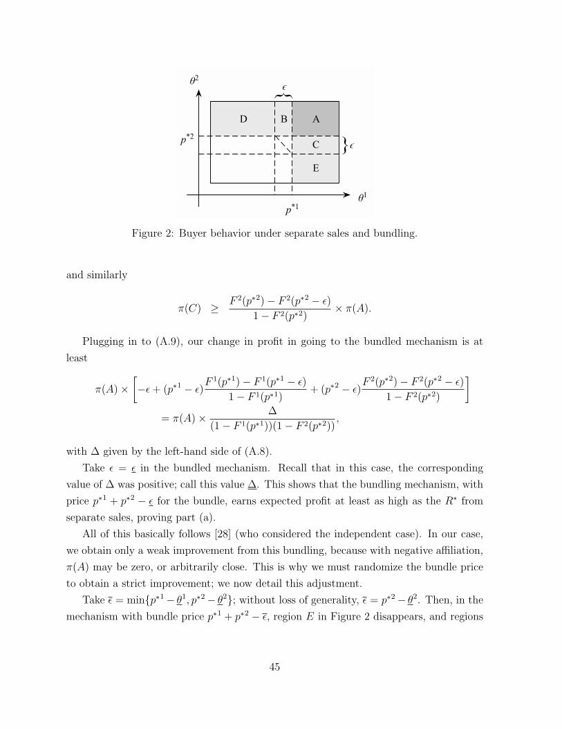
AB
C
D
E
p*1
p*2
θ1
θ2 {
{
ϵ
ϵ
Figure 2: Buyer behavior under separate sales and bundling.
and similarly
π(C) ≥F 2(p∗2)− F 2(p∗2 − ǫ)
1− F 2(p∗2)× π(A).
Plugging in to (A.9), our change in profit in going to the bundled mechanism is at
least
π(A)×
[−ǫ+ (p∗1 − ǫ)
F 1(p∗1)− F 1(p∗1 − ǫ)
1− F 1(p∗1)+ (p∗2 − ǫ)
F 2(p∗2)− F 2(p∗2 − ǫ)
1− F 2(p∗2)
]
= π(A)×∆
(1− F 1(p∗1))(1− F 2(p∗2)),
with ∆ given by the left-hand side of (A.8).
Take ǫ = ǫ in the bundled mechanism. Recall that in this case, the corresponding
value of ∆ was positive; call this value ∆. This shows that the bundling mechanism, with
price p∗1 + p∗2 − ǫ for the bundle, earns expected profit at least as high as the R∗ from
separate sales, proving part (a).
All of this basically follows [28] (who considered the independent case). In our case,
we obtain only a weak improvement from this bundling, because with negative affiliation,
π(A) may be zero, or arbitrarily close. This is why we must randomize the bundle price
to obtain a strict improvement; we now detail this adjustment.
Take ǫ = min{p∗1 − θ1, p∗2 − θ2}; without loss of generality, ǫ = p∗2 − θ2. Then, in the
mechanism with bundle price p∗1 + p∗2 − ǫ, region E in Figure 2 disappears, and regions
45

A and C constitute all of the area to the right of the line θ1 = p∗1, implying
π(C) = (1− F 1(p∗1))− π(A).
Therefore, expression (A.9) is at least
−ǫπ(A) + (p∗2 − ǫ)[(1− F 1(p∗1))− π(A)]
= θ2(1− F 1(p∗1))− p∗2π(A).
Consequently, if ǫ is chosen to equal ǫ with probability q and ǫ with probability 1− q, the
expected gain in profit relative to separate prices is at least
q∆
(1− F 1(p∗1))(1− F 2(p∗2))π(A) + (1− q)
(θ2(1− F 1(p∗1))− p∗2π(A)
)
= (1− q)θ2(1− F 1(p∗1)) + π(A)
[q
∆
(1− F 1(p∗1))(1− F 2(p∗2))− (1− q)p∗2
].
Evidently, if q is chosen close enough to 1, the expression in brackets on the right will be
positive. Then, for any negatively affiliated distribution π, the profit from the randomized
bundling mechanism will be at least R∗ + (1− q)θ2(1− F 1(p∗1)), which is strictly above
R∗, proving part (b).
Proof of Lemma 5.2. For each good g, write Θg = {θg1, . . . , θgrg}, with the values listed
in increasing order, θg1 < · · · < θgrg . By assumption, the optimal price to sell good g is
unique, and clearly it must equal one of the values θgj ; write j∗g for the index, so that the
optimal price is θgj∗g . We will also refer to this price as simply θ∗g.
Any joint screening mechanism in this environment can be represented by |Θ| · (G+1)
numbers: xg(θ) ∈ [0, 1], the probability that type θ receives good g, for each g and θ; and
t(θ), the payment made by type θ. Write (x∗, t∗) for the mechanism that sells each good
g separately at price θgj∗g .
Let Sg be the collection of all subsets of Θg that contain θgj∗g . For each such subset
Θg ∈ Sg, let πg[Θg] be some distribution in the corresponding one-good problem whose
support is Θg, and for which the unique optimal mechanism is a posted price of θgj∗g . (This
can be constructed, for example, by placing large enough probability mass on θgj∗g .) Now,
by choosing a sufficiently small positive weight ηg[Θg] for each Θg ∈ Sg, we can write πg
46
as a convex combination of distributions
πg =∑
Θg∈Sg
ηg[Θg]πg[Θg] + ηg[∅]πg (A.10)
where πg is some distribution that still has full support on Θg, and still has the property
that the unique optimal price is θgj∗g . For convenience, write Sg= Sg∪{∅} and πg[∅] = πg;
this allows us to write more simply
πg =∑
Θg∈Sg
ηg[Θg]πg[Θg]. (A.11)
Let S = ×g Sg. Consider any choice of Θ = (Θ1, . . . , ΘG) ∈ S. We know that
for each separate good g, setting a price of θgj∗g for each item is optimal against each
marginal distribution πg[Θg]. Accordingly, let π[Θ] be the joint distribution constructed
in Subsection 4.2, so that its marginals are the distributions πg[Θg] and such that (x∗, t∗)
is an optimal mechanism for distribution π[Θ].
Then, we can define a joint distribution π on Θ by
π =∑
Θ∈S
(G∏
g=1
ηg[Θg]
)π[Θ].
It is straightforward to check, using (A.11) that π is a distribution on Θ whose marginal
on each Θg equals πg; and (x∗, t∗) is an optimal mechanism for distribution π. We will
show that in fact (x∗, t∗) is the unique optimal mechanism for π.
First, we check that π has full support on Θ. Note that for this, it suffices to check
that whenever Θ is chosen with each Θg consisting of θgj∗g and at most one other value,
then π[Θ] has full support on Θ1 × · · · × ΘG; this is sufficient since every element of Θ
belongs to some such product set Θ.
To accomplish this, we look explicitly at the construction in Subsection 4.2. For each
of the corresponding (one-dimensional) component problems Θg, if |Θg| = 2, then the
standard analysis of the component screening problem tells us that the IR constraint of
the low type and the IC for the high type to imitate the low type both have positive
multipliers in the LP. (If |Θg| = 1 then the IR constraint of the one type likewise has
a positive multiplier.) Now we can easily check that π[Θ] places positive probability on
every θ ∈ Θ, by “upward induction.” Note that π[Θ](θ) = γg(θ) · πg[Θg](θg) is positive if
γg(θ) is positive for any g, which will happen if the right side of (4.16) is positive for that
47
type θ; and moreover once this happens, then γg(θ) must be positive for every g. If θ is
the lowest type in Θ, then the term κ[θ] is positive (in fact it equals 1) and so the right side
is positive. If not, then find some component h such that θh is the higher type in Θh, and
let θh be the lower type in Θh. Then, by the induction hypothesis, γh[θh, θ−h] > 0, and
also λh[θh → θh] > 0 from the component problem as already observed. Consequently,
the h-term in the sum on the right side of (4.16) is positive, giving the induction step.
This completes the verification that each such π[Θ] has full support, and so π does as
well.
Now back to our main event. Let (x, t) be any optimal mechanism for π; we wish to
show that it fully coincides with (x∗, t∗). Since Eπ[Θ][t(θ)] ≤ Eπ[Θ][t∗(θ)] for each π[Θ],
the only way t can obtain the same expected profit as t∗ against π is to have equality
for every π[Θ], i.e. (x, t) must be an optimal mechanism for every distribution π[Θ]. In
particular, it must satisfy the IR constraint with equality for the lowest type in Θ, by the
usual argument: if this constraint were slack, then it would be slack for every type in Θ
(since the agent’s utility for any allocation is increasing in his type), and so by increasing
the payment of every type by a small amount ǫ, we could construct a new mechanism
that earns strictly better profit against π[Θ].
But every θ ∈ Θ that is componentwise less than or equal to θ∗ = (θ1j∗1
, . . . , θgj∗g) is the
lowest type in some Θ. Consequently, this type must receive payoff 0 in the mechanism
(x, t).
We now show that any such type θ must receive zero quantity of every good g for
which θg < θ∗g. Indeed, the IC constraint for type θ∗ to imitate θ gives
∑
g
θ∗gxg(θ∗)− t(θ∗) ≥∑
g
θ∗gxg(θ)− t(θ) =
(∑
g
θgxg(θ)− t(θ)
)+∑
g
(θ∗g − θg)xg(θ).
But the left side is zero, by binding IR. Since every term on the right side is nonnegative,
they must all be zero, and in particular xg(θ) = 0 for every good g where θg < θ∗g strictly.
It follows that for every θ that is componentwise ≤ θ∗g, the only goods that this type
can be allocated by the mechanism are those for which θg = θ∗g, and so∑
g θgxg(θ) ≤
∑g:θg=θ∗g θ
∗g. Hence, IR implies t(θ) is at most∑
g:θg=θ∗g θ∗g. But this is exactly what
type θ pays in the separate-sales mechanism (x∗, t∗). Moreover, type θ is only willing to
pay this much if it is given the full allocation of all goods g with θg = θ∗g, i.e. xg(θ) = 1
for each such g. Thus, we have t(θ) ≤ t∗(θ) for each such θ, and if equality holds then
x(θ) = x∗(θ).
48
On the other hand, the full-support argument above now implies that we must indeed
have t(θ) = t∗(θ) for each such θ, because otherwise (x, t) would earn strictly lower
expected profit than (x∗, t∗) against some distribution π[Θ]. Hence, we have shown that
(x, t) coincides with (x∗, t∗) for all types that are ≤ θ∗ componentwise.
Now consider any θ that is componentwise greater than or equal to θ∗. Type θ can, by
imitating θ∗, buy every good g at price θ∗g, and so earn a payoff of∑
g(θg − θ∗g). Since
the total surplus available is∑
g θg, the largest amount t(θ) that the principal can extract
from such a type is∑
g θ∗g = t∗(θ). That is, we have t(θ) ≤ t∗(θ) for all such types, and
equality is possible only if x(θ) = x∗(θ). As before, full support implies we must have
t(θ) = t∗(θ) for all such types, and so (x, t) agrees with (x∗, t∗) on these types.
Finally, it remains to consider the types θ that have θg < θ∗g for at least one good
and θg > θ∗g for at least one good. For any such θ, define types θ− and θ+ by
θ−g= min{θg, θ∗g}, θ+
g= max{θg, θ∗g} for all g.
Considering the incentives of θ+ to imitate θ, the incentives of θ to imitate θ−, and
the binding IR for type θ− (which was already shown), we have
∑
g
θ+gxg(θ+)− t(θ+) ≥
∑
g
θ+gxg(θ)− t(θ)
=
(∑
g
θgxg(θ)− t(θ)
)+∑
g
(θ+g− θg)xg(θ)
≥
(∑
g
θgxg(θ−)− t(θ−)
)+∑
g
(θ+g− θg)xg(θ)
≥
(∑
g
θ−gxg(θ−)− t(θ−)
)+∑
g
(θ+g− θg)xg(θ) +
∑
g
(θg − θ−g)xg(θ−)
=∑
g
(θ+g− θg)xg +
∑
g
(θg − θ−g)xg(θ−).
But we already have established that (x, t) coincides with (x∗, t∗) at θ− and θ+, and
so we can plug in on the left side and in the last sum on the right side, obtaining
∑
g:θg≥θ∗g
(θg − θ∗g) ≥∑
g
(θ+g− θg)xg(θ) +
∑
g:θg≥θ∗g
(θg − θ∗g).
49
Since∑
g(θ+g − θg)xg(θ) ≥ 0, we must have equality throughout. In particular, this
implies that xg(θ) = 0 for each g with θg < θ∗g. Then, once this is established, the
incentive to imitate type θ− implies (after transposing)
t(θ) ≤∑
g
θgxg(θ)−
(∑
g
θgxg(θ−)− t(θ−)
)
=∑
g:θg≥θ∗g
θg(xg(θ)− 1) + t(θ−)
≤ t(θ−)
= t∗(θ−)
= t∗(θ)
where the second-last equality holds because we already saw that t and t∗ coincide at all
types below θ∗, and the last equality holds because, in mechanism (x∗, t∗), both θ− and
θ buy exactly the goods for which θg ≥ θ∗g. Thus we see that t(θ) ≤ t∗(θ), and as usual,
equality can only hold if x(θ) = x∗(θ).
At this point we have shown that t(θ) ≤ t∗(θ) for every possible θ. By the full-support
argument again, equality must hold everywhere, which in turn implies x(θ) = x∗(θ) for
every θ as well.
References
[1] William James Adams and Janet L. Yellen (1976), “Commodity Bundling and the
Burden of Monopoly,” Quarterly Journal of Economics 90 (3), 475–498.
[2] Mark Armstrong (1996), “Multiproduct Nonlinear Pricing,” Econometrica 64 (1),
51–75.
[3] Mark Armstrong (1999), “Price Discrimination by a Many-Product Firm,” Review
of Economic Studies 66 (1), 151–168.
[4] Yannis Bakos and Erik Brynjolfsson (1999), “Bundling Information Goods: Pricing,
Profits, and Efficiency,” Management Science 45 (12), 1613–1630.
50

[5] Erik J. Balder (1996), “On the Existence of Optimal Contract Mechanisms for In-
complete Information Principal-Agent Models,” Journal of Economic Theory 68 (1),
133–148.
[6] Marco Battaglini and Rohit Lamba (2014), “Optimal Dynamic Contracting: the
First-Order Approach and Beyond,” working paper, Princeton University.
[7] Dirk Bergemann and Stephen Morris (2005), “Robust Mechanism Design,” Econo-
metrica 73 (6), 1771–1813.
[8] Moshe Babaioff, Nicole Immorlica, Brendan Lucier, and S. MatthewWeinberg (2014),
“A Simple and Approximately Optimal Mechanism for an Additive Buyer,” in Pro-
ceedings of the IEEE 55th Symposium on Foundations of Computer Science (FOCS
’14), 21–30.
[9] Benjamin Brooks (2013), “Surveying and Selling: Belief and Surplus Extraction in
Auctions,” working paper, University of Chicago.
[10] Vincent Conitzer and Tuomas Sandholm (2002), “Complexity of Mechanism Design,”
in Proceedings of the 18th Conference on Uncertainty in Artificial Intelligence (UAI
’02), 103–110.
[11] Gabriel Carroll (2012), “Robust Incentives for Information Acquisition,” working
paper, Stanford University.
[12] Gabriel Carroll (2015), “Robustness and Linear Contracts,” American Economic
Review 105 (2), 536–563.
[13] Kim-Sau Chung and J. C. Ely (2007), “Foundations of Dominant-Strategy Mecha-
nisms,” Review of Economic Studies 74 (2), 447–476.
[14] Constantinos Daskalakis, Alan Deckelbaum, and Christos Tzamos (2013), “Mecha-
nism Design via Optimal Transport,” in Proceedings of the 14th ACM Conference on
Electronic Commerce (EC ’13), 269–286.
[15] Constantinos Daskalakis, Alan Deckelbaum, and Christos Tzamos (2014), “Complex-
ity of Optimal Mechanism Design,” in Proceedings of the 25th Annual ACM-SIAM
Symposium on Discrete Algorithms (SODA ’14), 1302–1318.
51
[16] Emmanuel Farhi and Ivan Werning (2013), “Insurance and Taxation over the Life
Cycle,” Review of Economic Studies 80 (2), 596–635.
[17] Sebastian Findeisen and Dominik Sachs (2015), “Redistribution and Insurance with
Simple Tax Instruments,” working paper, University of Mannheim.
[18] Alexander Frankel (2014), “Aligned Delegation,” American Economic Review 104
(1), 66–83.
[19] Daniel Garrett (2014), “Robustness of Simple Menus of Contracts in Cost-Based
Procurement,” Games and Economic Behavior 87, 631–641.
[20] Nima Haghpanah and Jason Hartline (2015), “Reverse Mechanism Design,” working
paper, Northwestern University.
[21] Sergiu Hart and Noam Nisan (2012), “Approximate Revenue Maximization with
Multiple Items,” working paper, Hebrew University of Jerusalem.
[22] Sergiu Hart and Noam Nisan (2013), “The Menu-Size Complexity of Auctions,”
working paper, Hebrew University of Jerusalem.
[23] Sergiu Hart and Philip J. Reny (2014), “Maximal Revenue with Multiple Goods:
Nonmonotonicity and Other Observations,” Theoretical Economics, forthcoming.
[24] Roger A. Horn and Charles R. Johnson (1985), Matrix Analysis, Cambridge Univer-
sity Press.
[25] Xinye Li and Andrew Chi-Chih Yao (2013), “On Revenue Maximization for Selling
Multiple Independently Distributed Items,” Proceedings of the National Academy of
Sciences 110 (28), 11232–11237.
[26] Alejandro M. Manelli and Daniel R. Vincent (2006), “Bundling as an Optimal Selling
Mechanism for a Multiple-Good Monopolist,” Journal of Economic Theory 127 (1),
1–35.
[27] Kristof Madarasz and Andrea Prat, “Sellers with Misspecified Models,” working
paper, London School of Economics.
[28] R. Preston McAfee, John McMillan, and Michael D. Whinston (1989), “Multiproduct
Monopoly, Commodity Bundling, and Correlation of Values,” Quarterly Journal of
Economics 104 (2), 371–383.
52
[29] Michael Mussa and Sherwin Rosen (1978), “Monopoly and Product Quality,” Journal
of Economic Theory 18 (2), 301–317.
[30] Roger B. Myerson (1981), “Optimal Auction Design,” Mathematics of Operations
Research 6 (1), 58–73.
[31] James M. Ortega (1987), Matrix Theory: A Second Course, Plenum Press.
[32] John Riley and Richard Zeckhauser (1983), “Optimal Selling Strategies: When to
Haggle, When to Hold Firm,” Quarterly Journal of Economics 98 (2), 267–289.
[33] Jean-Charles Rochet and Lars A. Stole (2003), “The Economics of Multidimensional
Screening,” in Advances in Economics and Econometrics: Theory and Applications,
Eighth World Congress, Vol. I, ed. Mathias Dewatripont, Lars Peter Hansen, and
Stephen J. Turnovsky, Cambridge University Press.
[34] Casey Rothschild and Florian Scheuer (2013), “Redistributive Taxation in the Roy
Model,” Quarterly Journal of Economics 128 (2), 623–668.
[35] Casey Rothschild and Florian Scheuer (2014), “A Theory of Income Taxation under
Multidimensional Skill Heterogeneity,” working paper, Stanford University.
[36] Ilya Segal (2003), “Optimal Pricing Mechanisms with Unknown Demand,” American
Economic Review 93 (3), 509–529.
[37] Stefanie Stantcheva (2015), “Optimal Taxation and Human Capital Policies over the
Life Cycle,” working paper, Harvard University.
[38] George J. Stigler (1963), “United States v. Loew’s Inc.: A Note on Block-Booking,”
Supreme Court Review, 152–157.
[39] Roland Strausz (2006), “Deterministic Versus Stochastic Mechanisms in Principal-
Agent Models,” Journal of Economic Theory 128 (1), 306–314.
[40] Zihe Wang and Pingzhong Tang (2014), “Optimal Mechanisms with Simple Menus,”
in Proceedings of the Fifteenth ACM Conference on Economics and Computation
(EC’14), 227–240.
[41] Gunter M. Ziegler (1995), Lectures on Polytopes, Graduate Texts in Mathematics
#152, Springer-Verlag, New York.
53


![QUASI-BIGEBRES DE LIE ET ALGEBRES QUASI-BATALIN ...streaming.ictp.it/preprints/P/99/174.pdf3 Quasi-bigebres de Lie Les quasi-bigebres de Lie [6] (appelees quasi-bigebres jacobiennes](https://img.pdfslide.us/doc/110x75/60aa5fd4a787df4f051abfc1/quasi-bigebres-de-lie-et-algebres-quasi-batalin-3-quasi-bigebres-de-lie-les.jpg)


![PERISHABLE DURABLE GOODSPERISHABLE DURABLE GOODS IN-KOO CHO Abstract. eW examine whether the Coase conjecture [7, 14, 4, 10] is robust against slight ability of commitment of the monopolist](https://img.pdfslide.us/doc/110x75/5eddd060ad6a402d666903d9/perishable-durable-goods-perishable-durable-goods-in-koo-cho-abstract-ew-examine.jpg)