Embed Size (px)
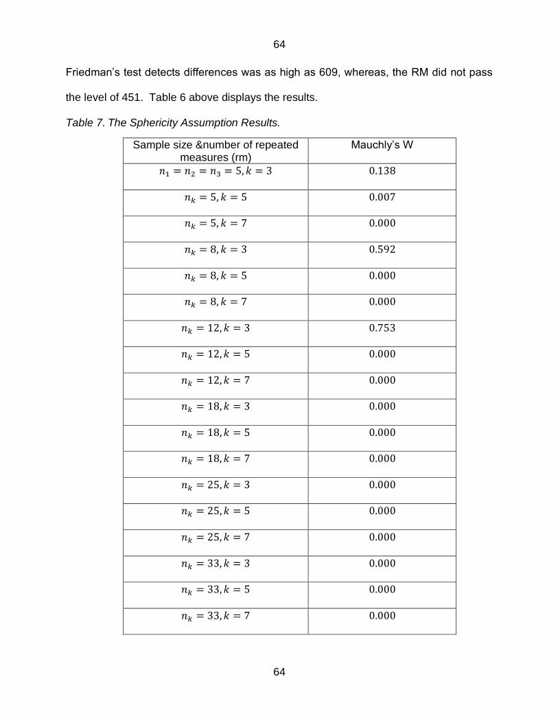
Citation preview

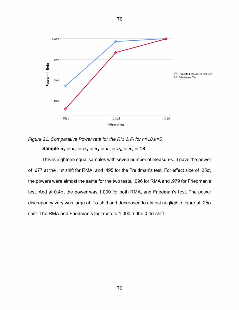
i
ROBUSTNESS AND COMPARATIVE STATISTICAL POWER OF THE REPEATED MEASURES ANOVA AND FRIEDMAN TEST WITH REAL DATA
By
OPEOLUWA BOLU FADEYI
DISSERTATION
Submitted to the Graduate School
Of Wayne State University
Detroit Michigan
In partial fulfillment of the requirements
for the degree of
DOCTOR OF PHILOSOPHY
2021
MAJOR EVALUATION AND RESEARCH
Approved by
____________________________________ Advisor Date
____________________________________
____________________________________
____________________________________
ii
DEDICATION
To my husband children and parents
iii
ACKNOWLEDGEMENTS
I would like to express my profound gratitude to my dissertation advisor Dr
Shlomo Sawilowsky for his insightful guidance It is difficult for me to comprehend how
he made out time to review my dissertation progressively and thoroughly His demise
was shocking and devastating as my study was concluding However he has written
his name in gold in my heart I sincerely appreciate Dr Barry Markman for all his
helpful comments and also for stepping out of retirement to chair my final defense
The course that I took with Dr Monte Piliawsky impacted the quality of my research
significantly On several instances Dr Aguwa reviewed my work and contributed
immensely to the richness of my research I am very grateful to these professors for
servin g on my dissertation committee
Also I will like to express my love and thankfulness to my husband Johnson
who spent sleepless nights with me proofreading my work Our children Wisdom
Delight and Goodness that endured a busy mom are much appreciated I sincerely
acknowledge several people that have been a part of my life during the doctoral study
who are too numerous to be included Above all I want to express my unquantifiable
gratitude to God His grace sustained and enabled me to reach the zenith of the
academic ladder
iv
TABLE OF CONTENTS
DEDICATION II
ACKNOWLEDGEMENTS III
LIST OF TABLES V
LIST OF FIGURES VII
CHAPTER ONE OVERVIEW OF THE PARAMETRIC TESTS 1
CHAPTER TWO THEORETICAL FOUNDATIONS AND LITERATURE REVIEW 11
CHAPTER THREE METHODOLOGY 46
CHAPTER FOUR RESULTS AND DISCUSSION 60
CHAPTER FIVE CONCLUSIONS AND IMPLICATIONS 90
APPENDIX A 98
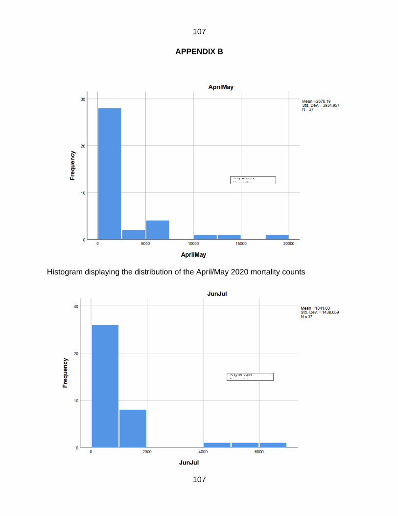
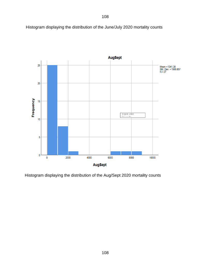
APPENDIX B 107
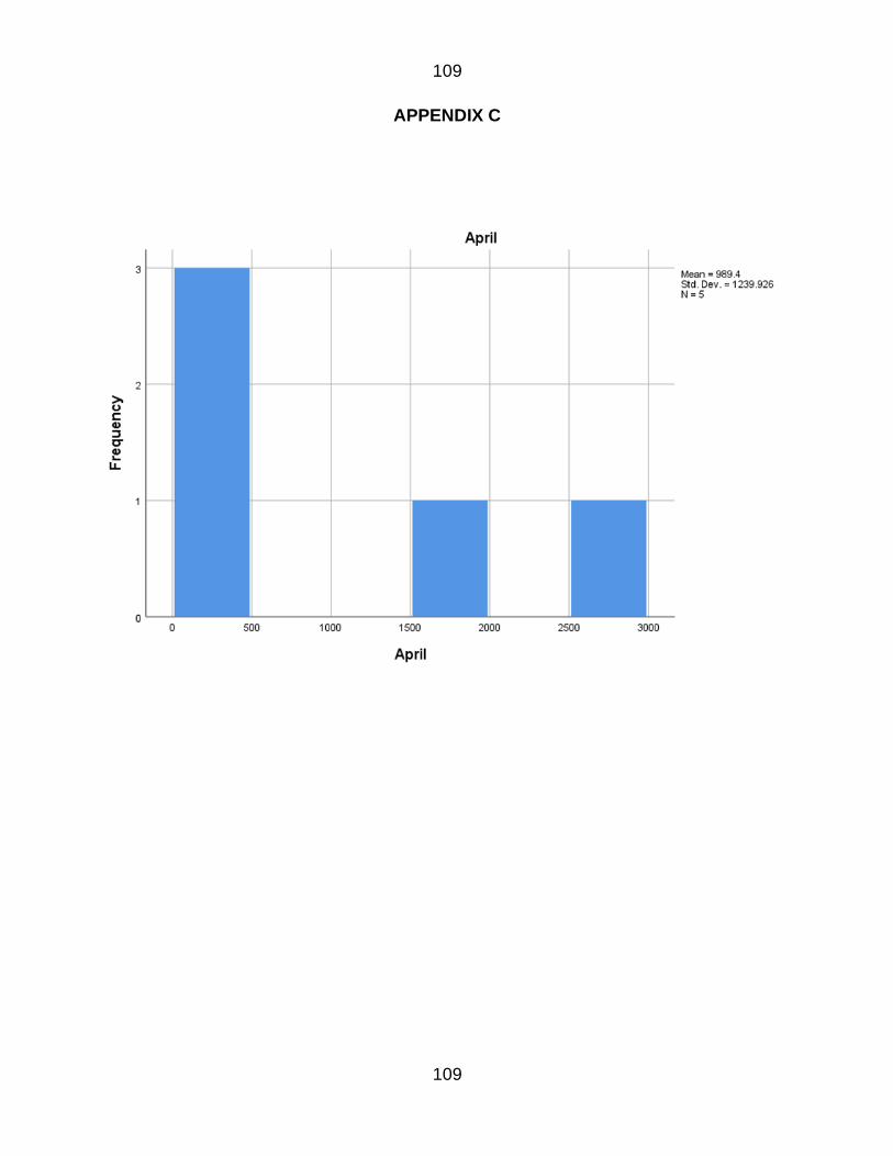
APPENDIX C 109
ABSTRACT 157
AUTOBIOGRAPHICAL STATEMENT 159
v
LIST OF TABLES
Table 1 Hypothesis Table 28
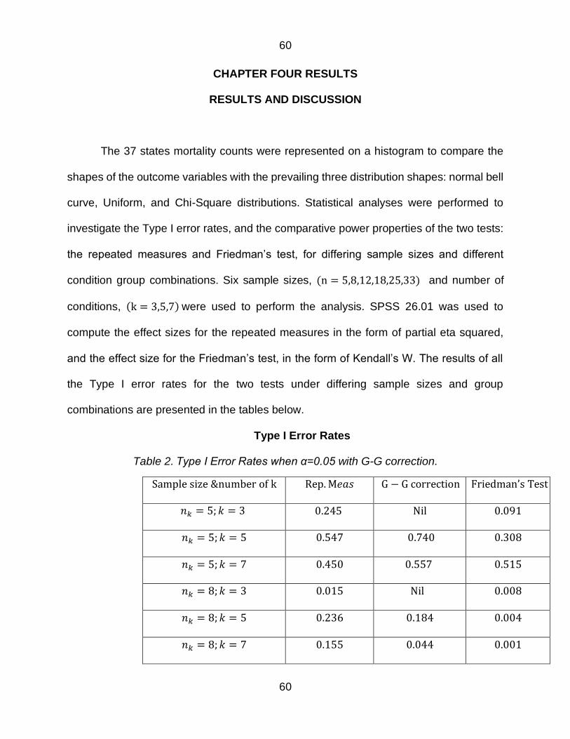
Table 2 Type I Error Rates when α=005 with G-G correction 60
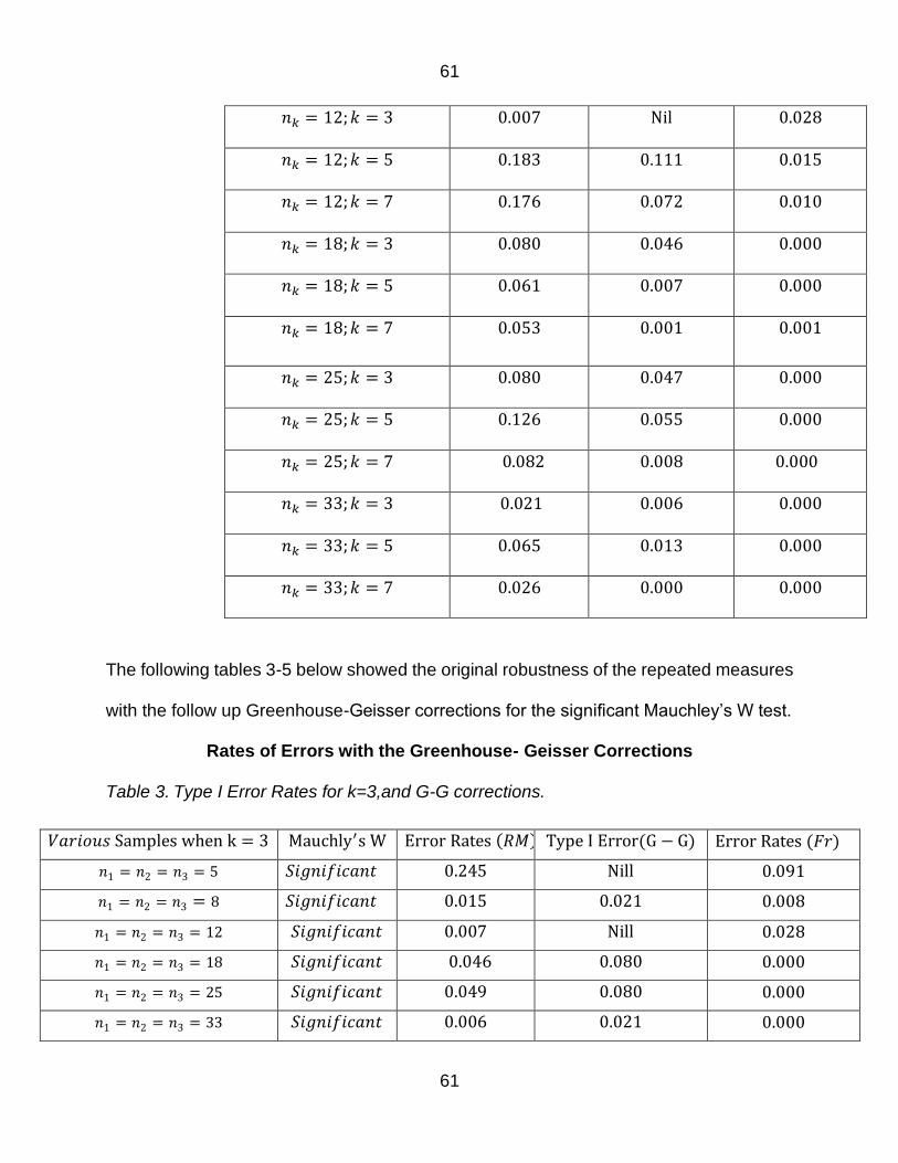
Table 3 Type I Error Rates for k=3and G-G corrections 61
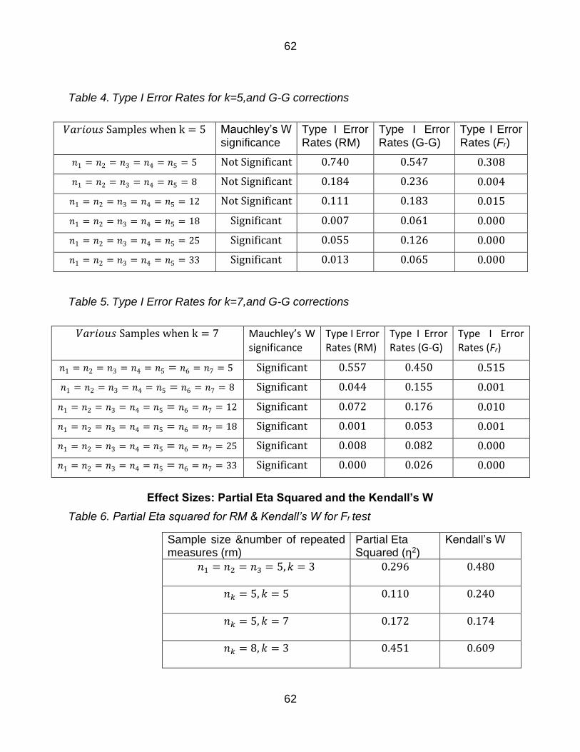
Table 4 Type I Error Rates for k=5and G-G corrections 62
Table 5 Type I Error Rates for k=7and G-G corrections 62
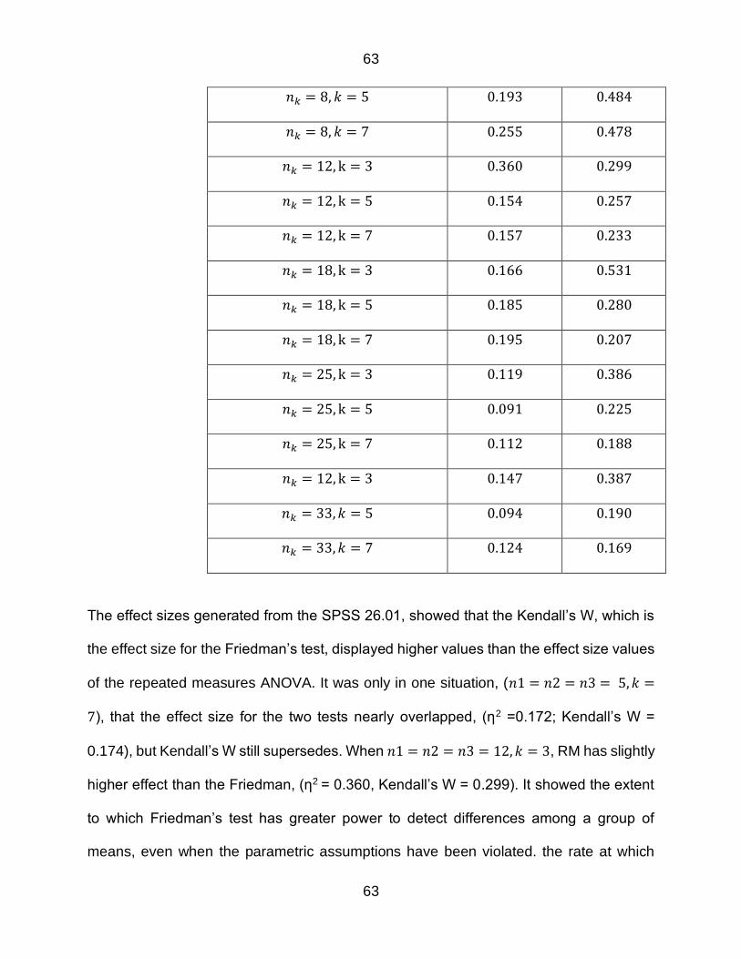
Table 6 Partial Eta squared for RM amp Kendallrsquos W for Fr test 62
Table 7 The Sphericity Assumption Results 64
Table 8 The power rates for n=5 k=3 83
Table 9 The power rates for n=8 k=3 83
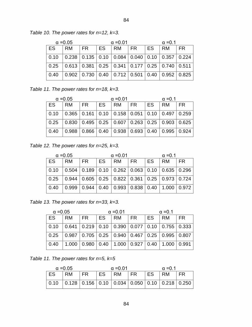
Table 10 The power rates for n=12 k=3 84
Table 14 The power rates for n=5 k=5 84
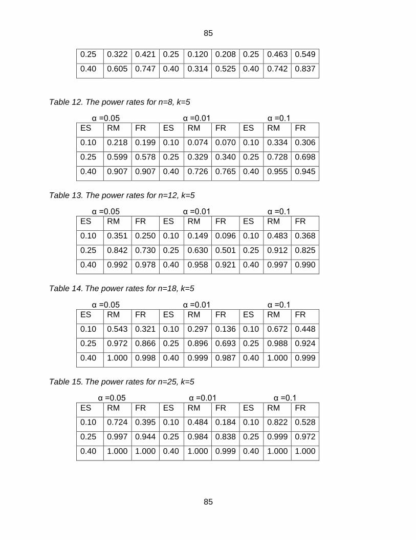
Table 15 The power rates for n=8 k=5 85
Table 16 The power rates for n=12 k=5 85
Table 17 The power rates for n=18 k=5 85
Table 18 The power rates for n=25 k=5 85
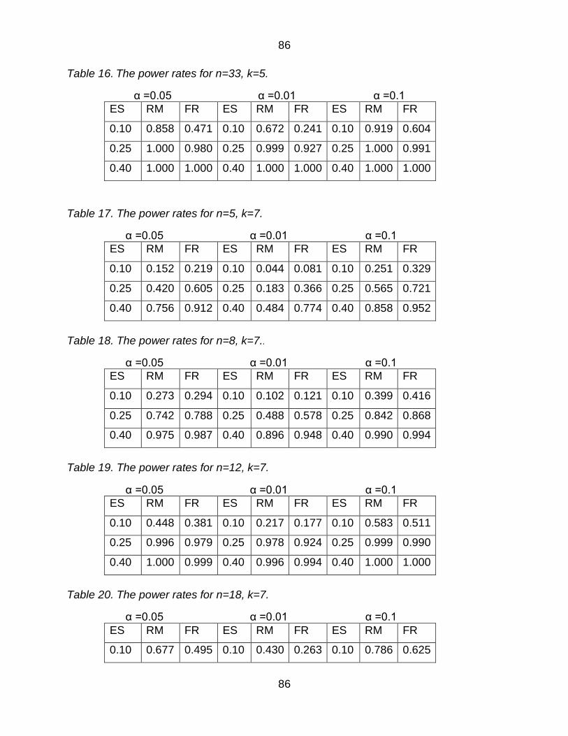
Table 19 The power rates for n=33 k=5 86
Table 20 The power rates for n=5 k=7 86
Table 21 The power rates for n=8 k=7 86
Table 22 The power rates for n=12 k=7 86
Table 23 The power rates for n=18 k=7 86
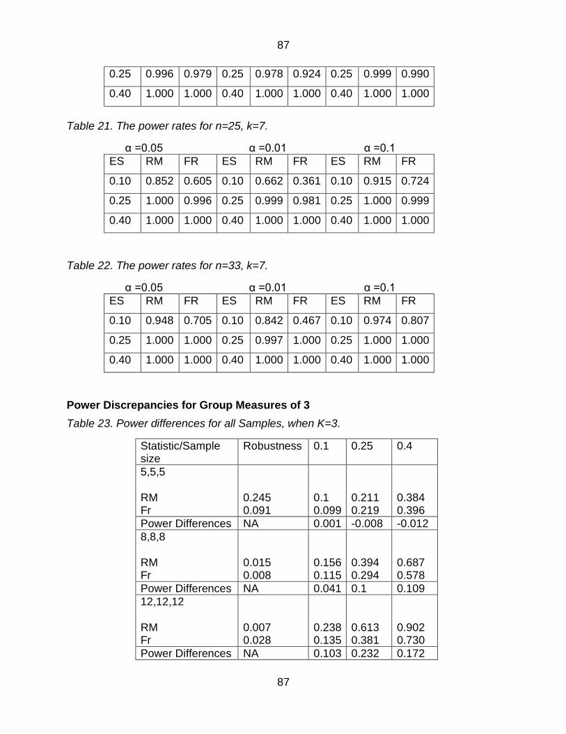
Table 24 The power rates for n=25 k=7 87
vi
Table 25 The power rates for n=33 k=7 87
Table 26 Power differences for all Samples when K=3 87
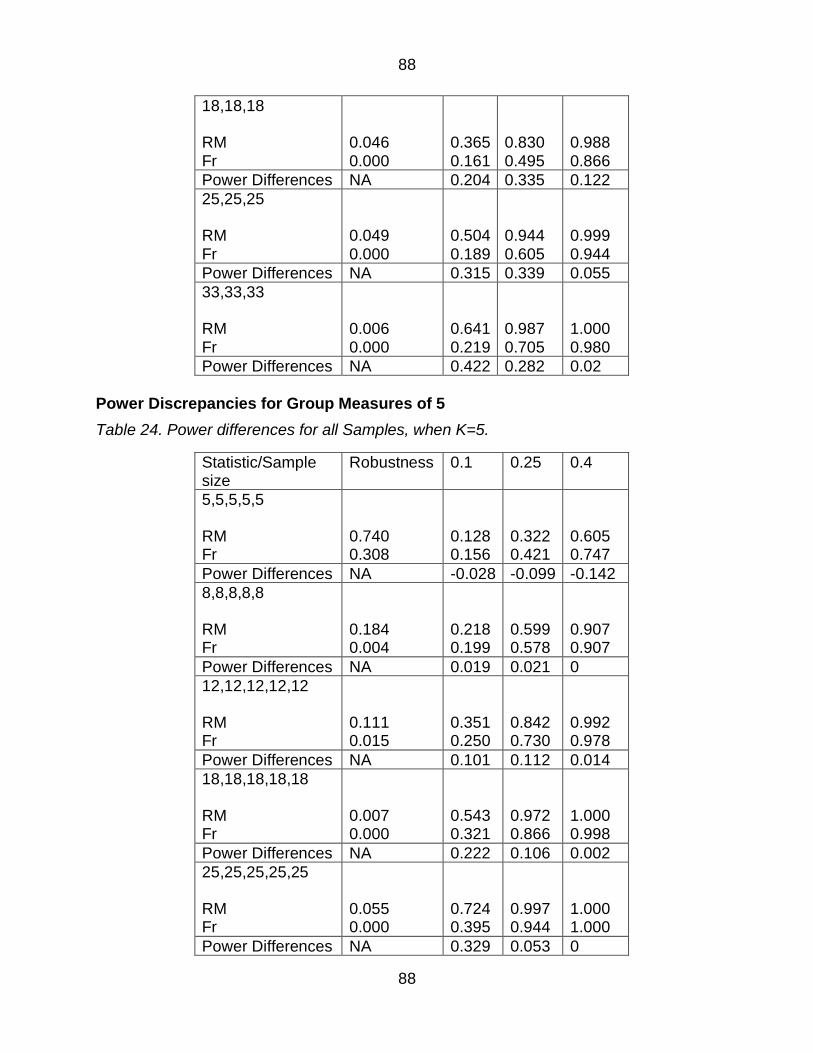
Table 27 Power differences for all Samples when K=5 88
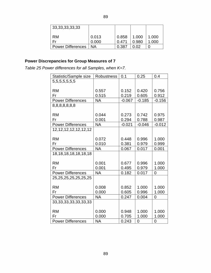
Table 28 Power differences for all Samples when K=7 89
vii
LIST OF FIGURES
Figure 1 Partition of Errors for One-factor Repeated Measures ANOVA 16
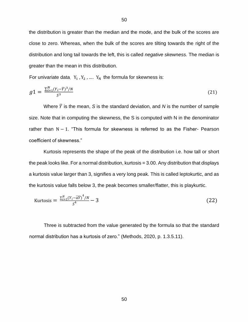
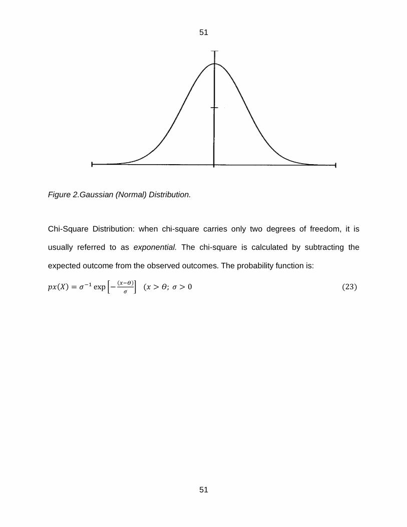
Figure 2Gaussian (Normal) Distribution 51
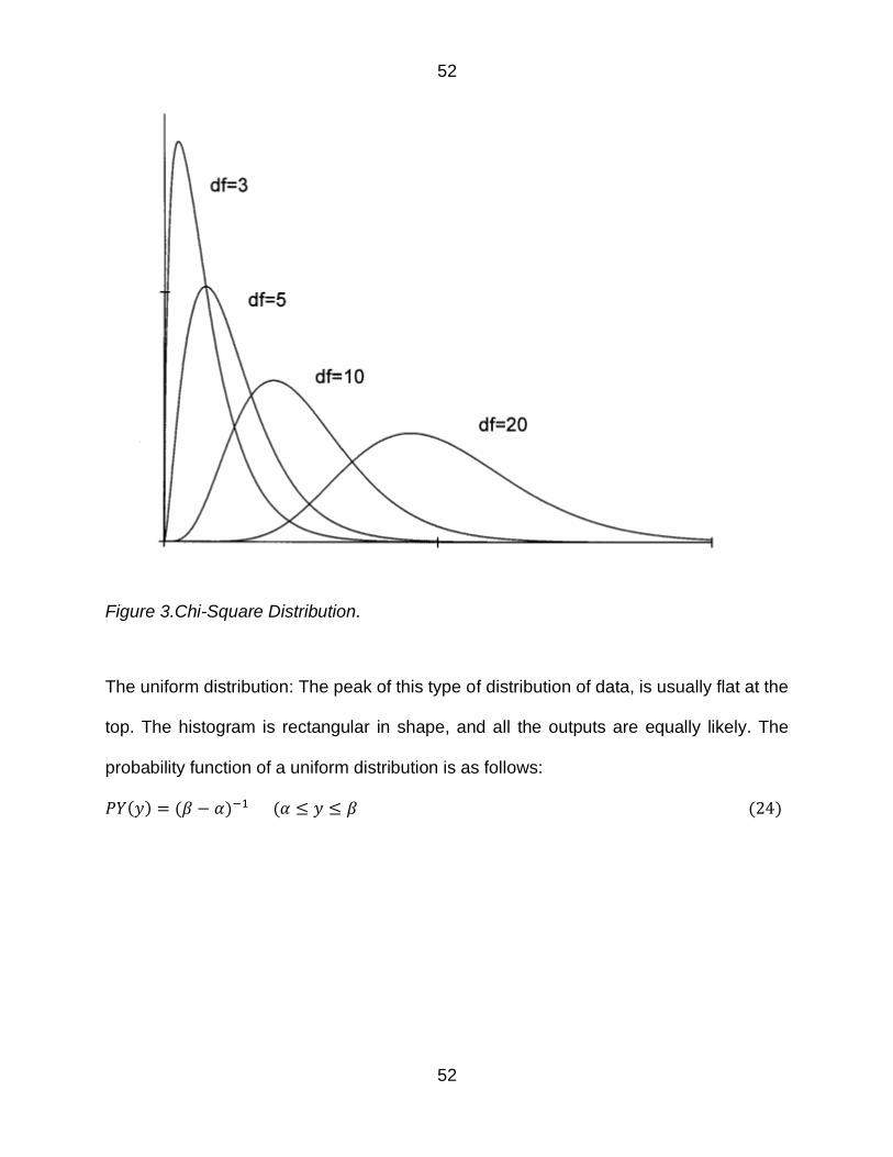
Figure 3Chi-Square Distribution 52
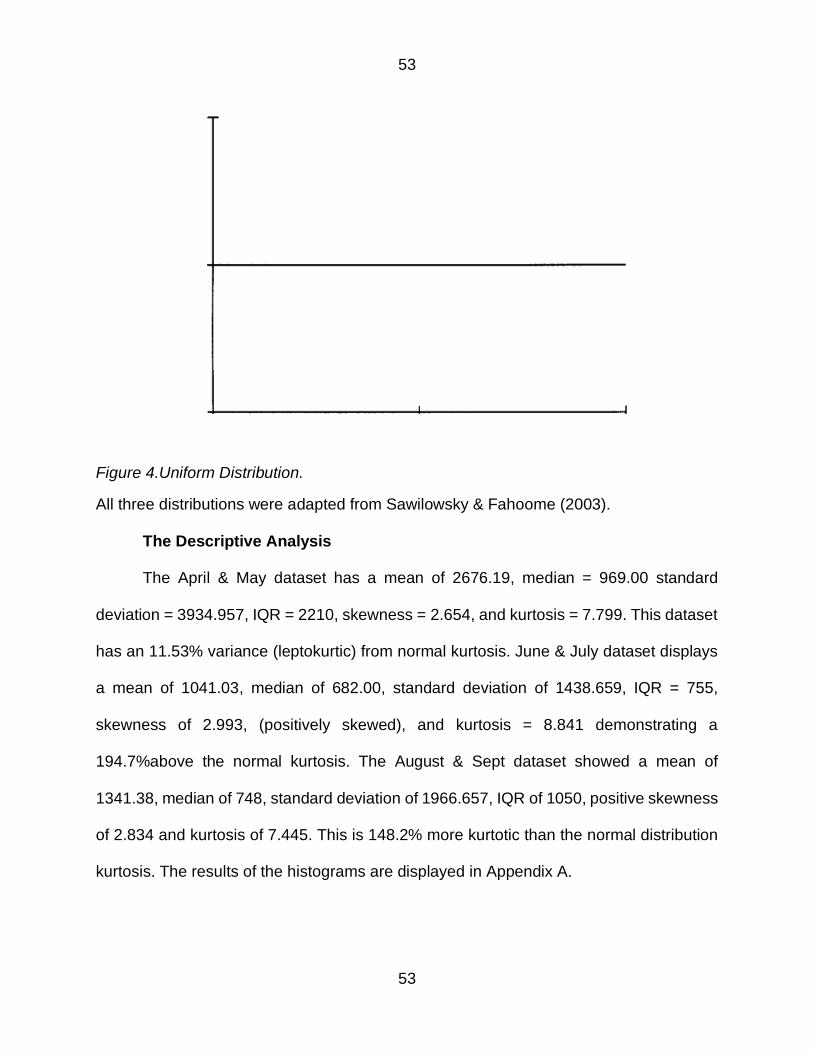
Figure 4Uniform Distribution 53
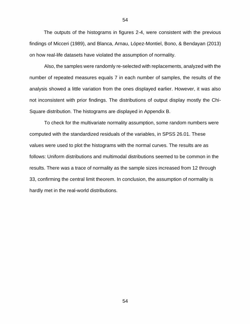
Figure 5 Multivariate Normal Distribution for Sample Size of 5 k=7 55
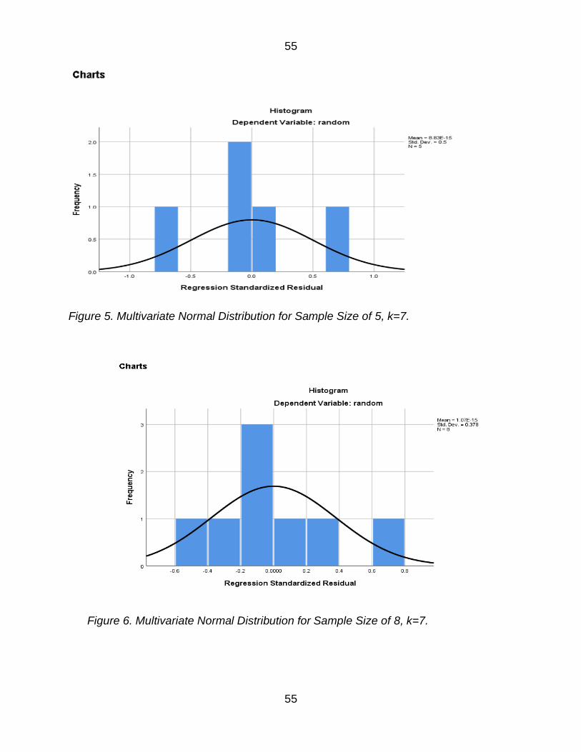
Figure 6 Multivariate Normal Distribution for Sample Size of 8 k=7 55
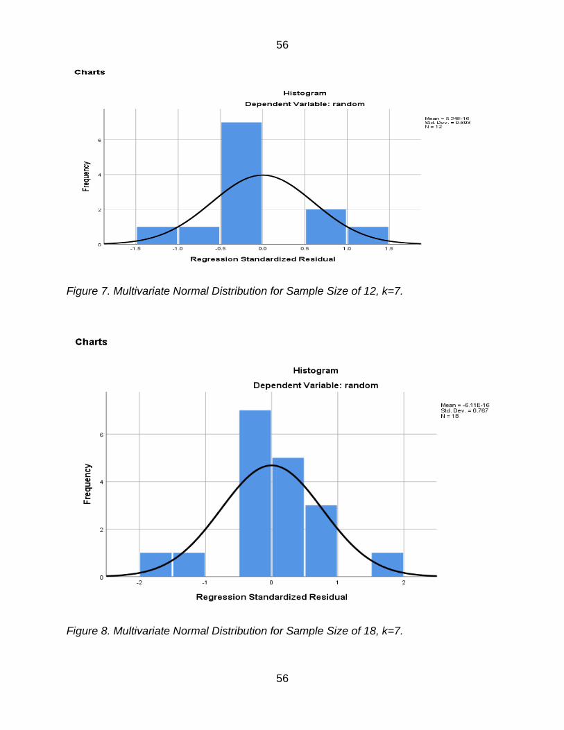
Figure 7 Multivariate Normal Distribution for Sample Size of 12 k=7 56
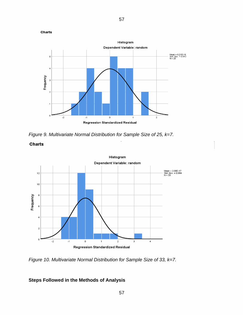
Figure 8 Multivariate Normal Distribution for Sample Size of 18 k=7 56
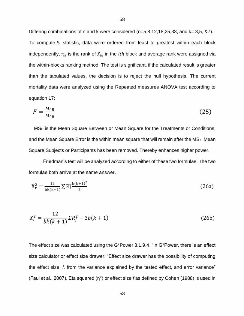
Figure 9 Multivariate Normal Distribution for Sample Size of 25 k=7 57
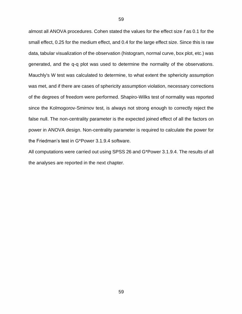
Figure 10 Multivariate Normal Distribution for Sample Size of 33 k=7 57
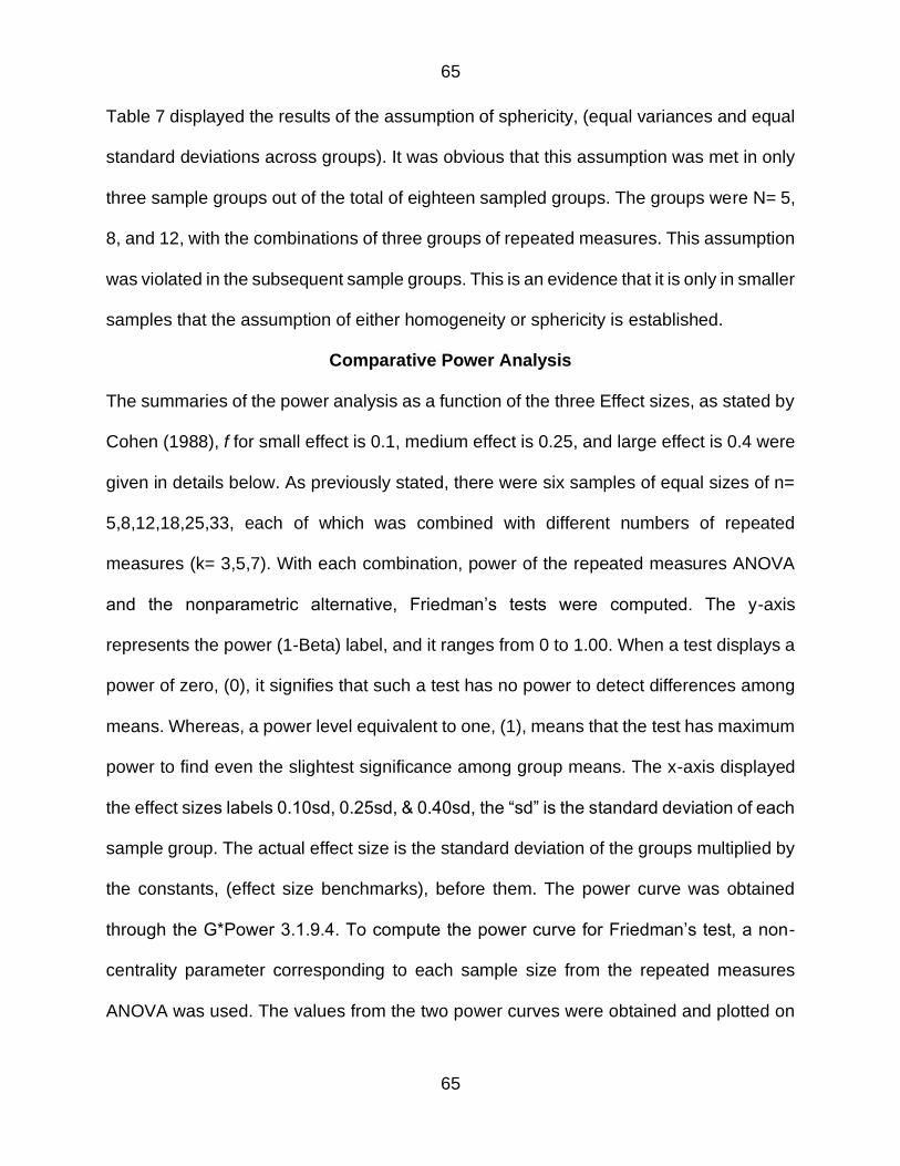
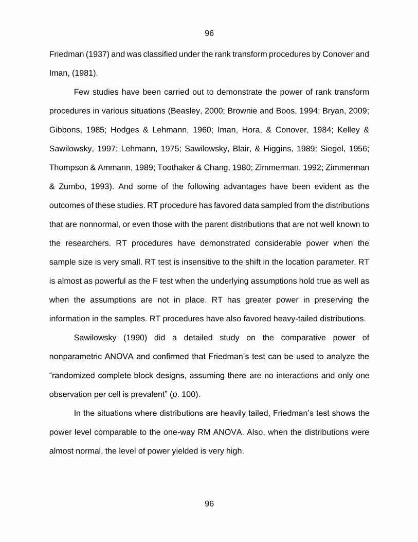
Figure 11 Comparative Power rate for the RM amp Fr for n=5k=3 66
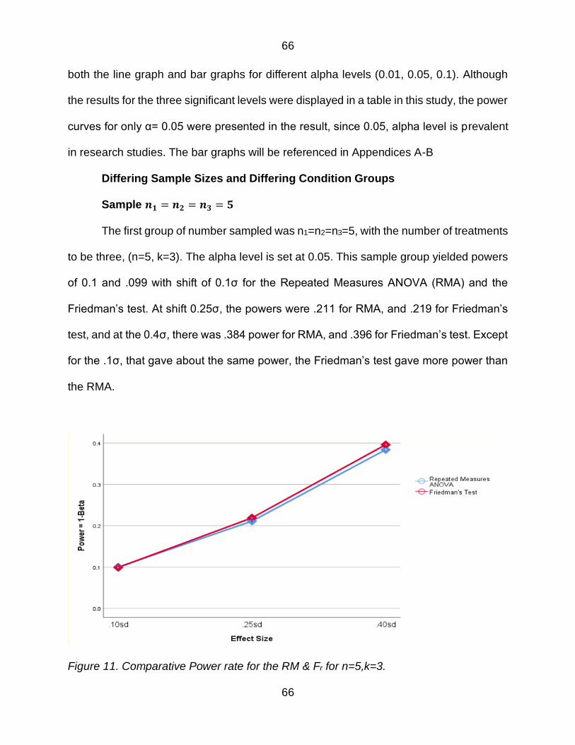
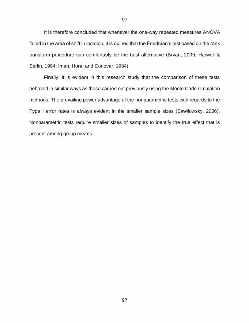
Figure 12 Comparative Power rate for the RM amp Fr for n=5k=5 67
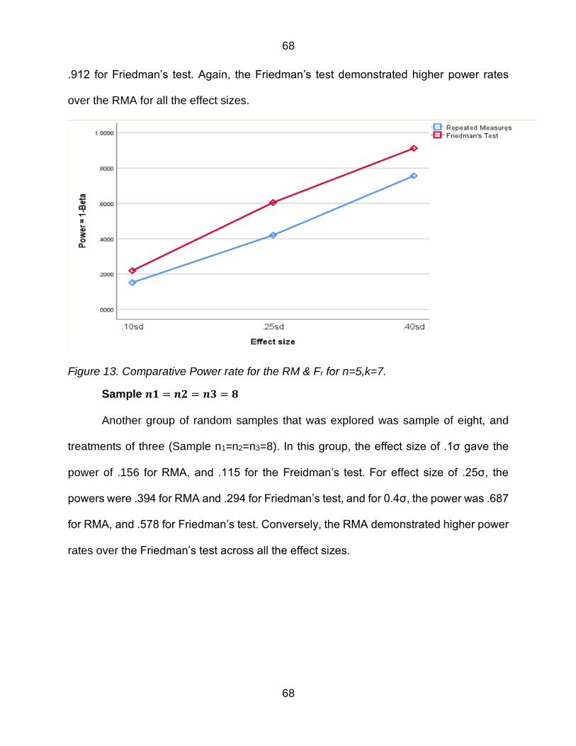
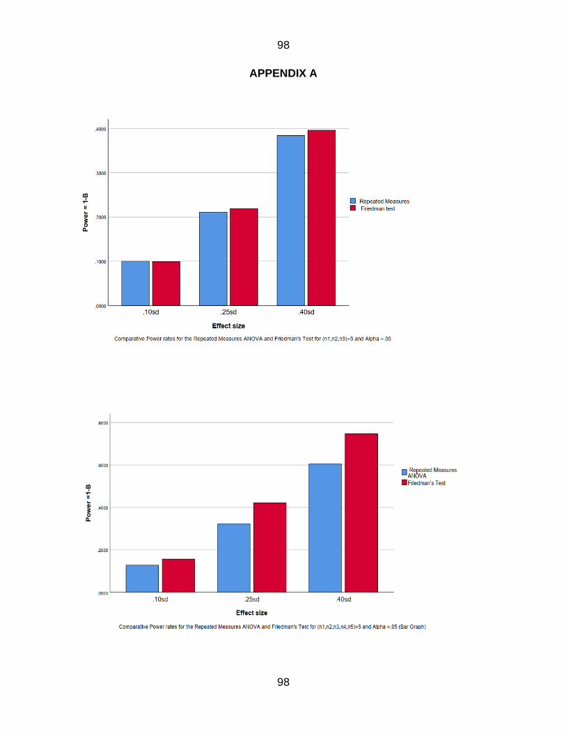
Figure 13 Comparative Power rate for the RM amp Fr for n=5k=7 68
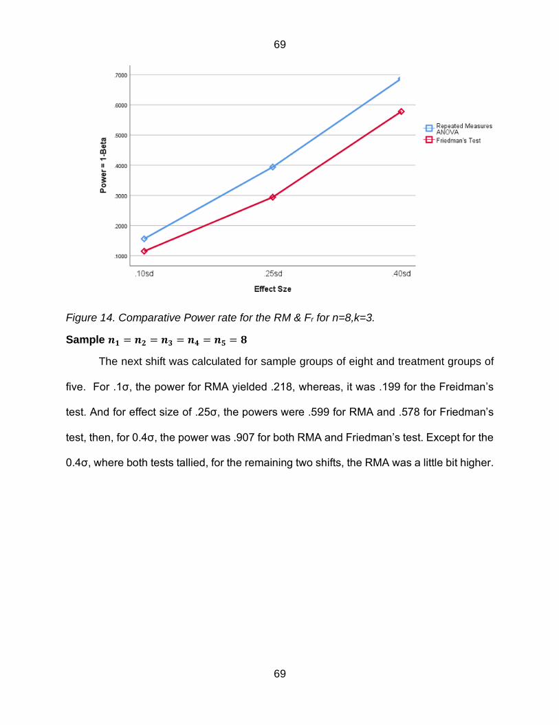
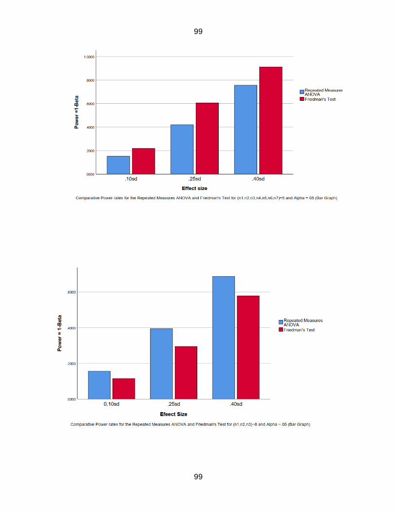
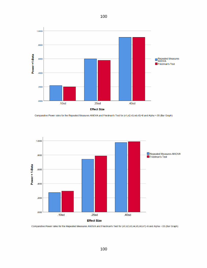
Figure 14 Comparative Power rate for the RM amp Fr for n=8k=3 69
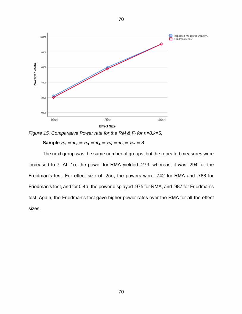
Figure 15 Comparative Power rate for the RM amp Fr for n=8k=5 70
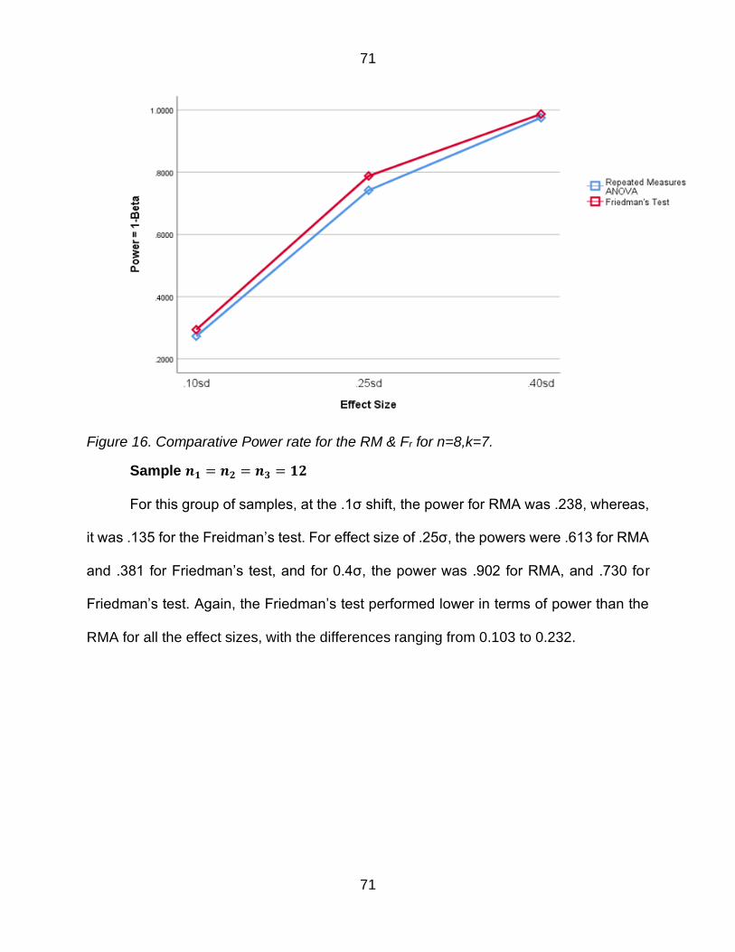
Figure 16 Comparative Power rate for the RM amp Fr for n=8k=7 71
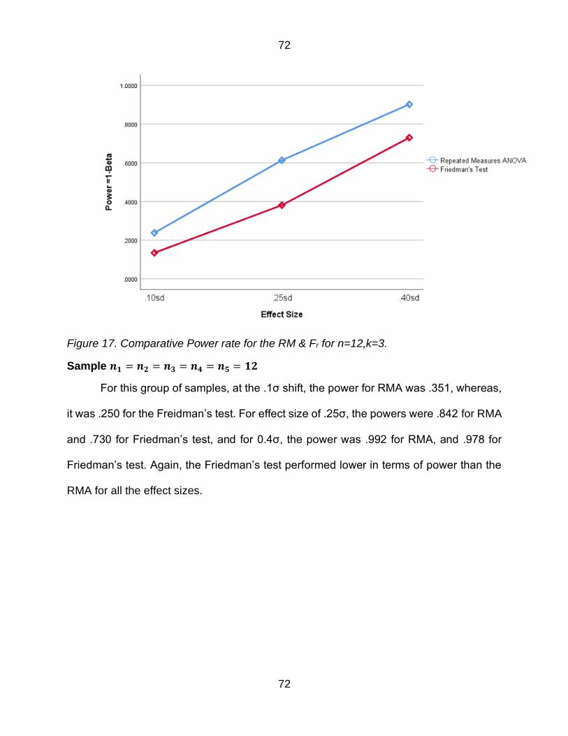
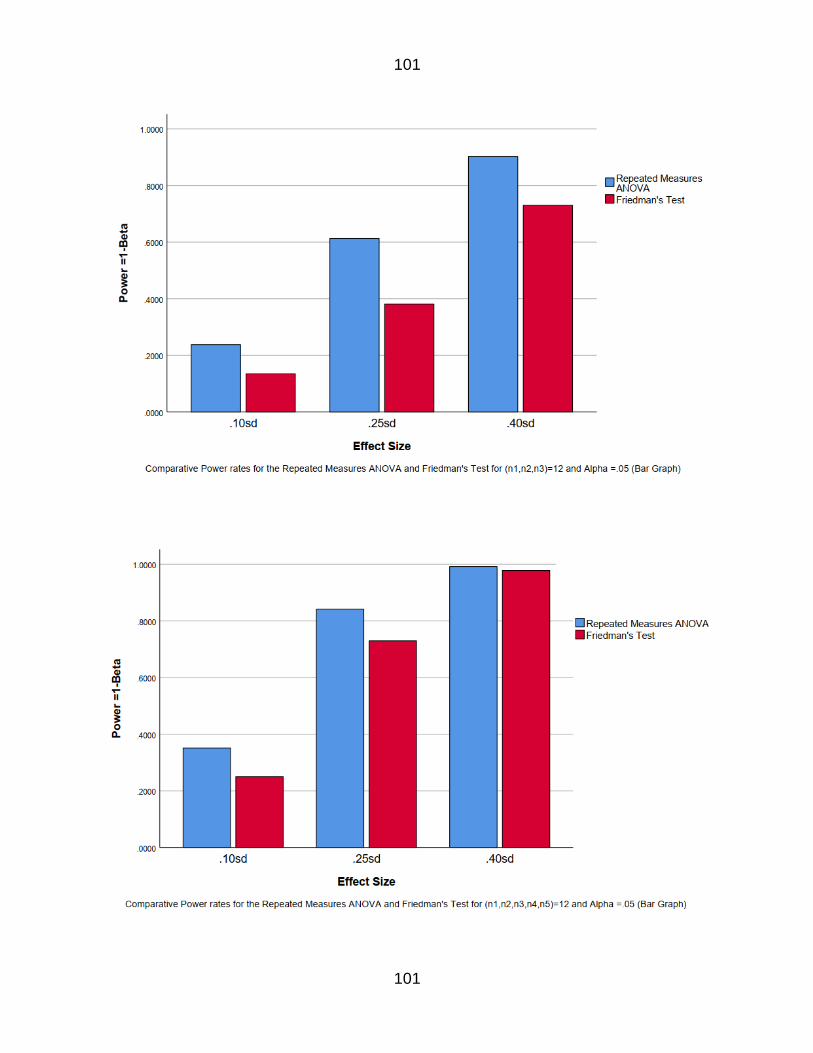
Figure 17 Comparative Power rate for the RM amp Fr for n=12k=3 72
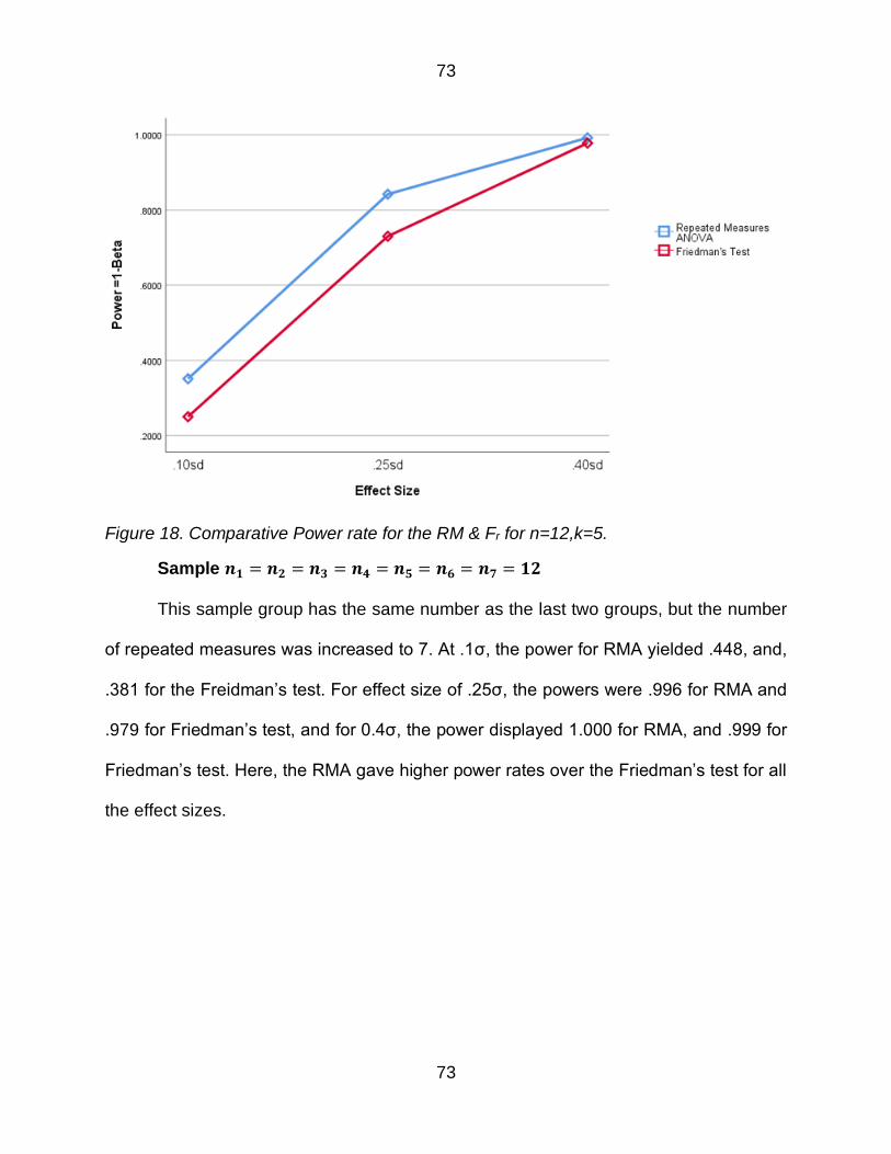
Figure 18 Comparative Power rate for the RM amp Fr for n=12k=5 73
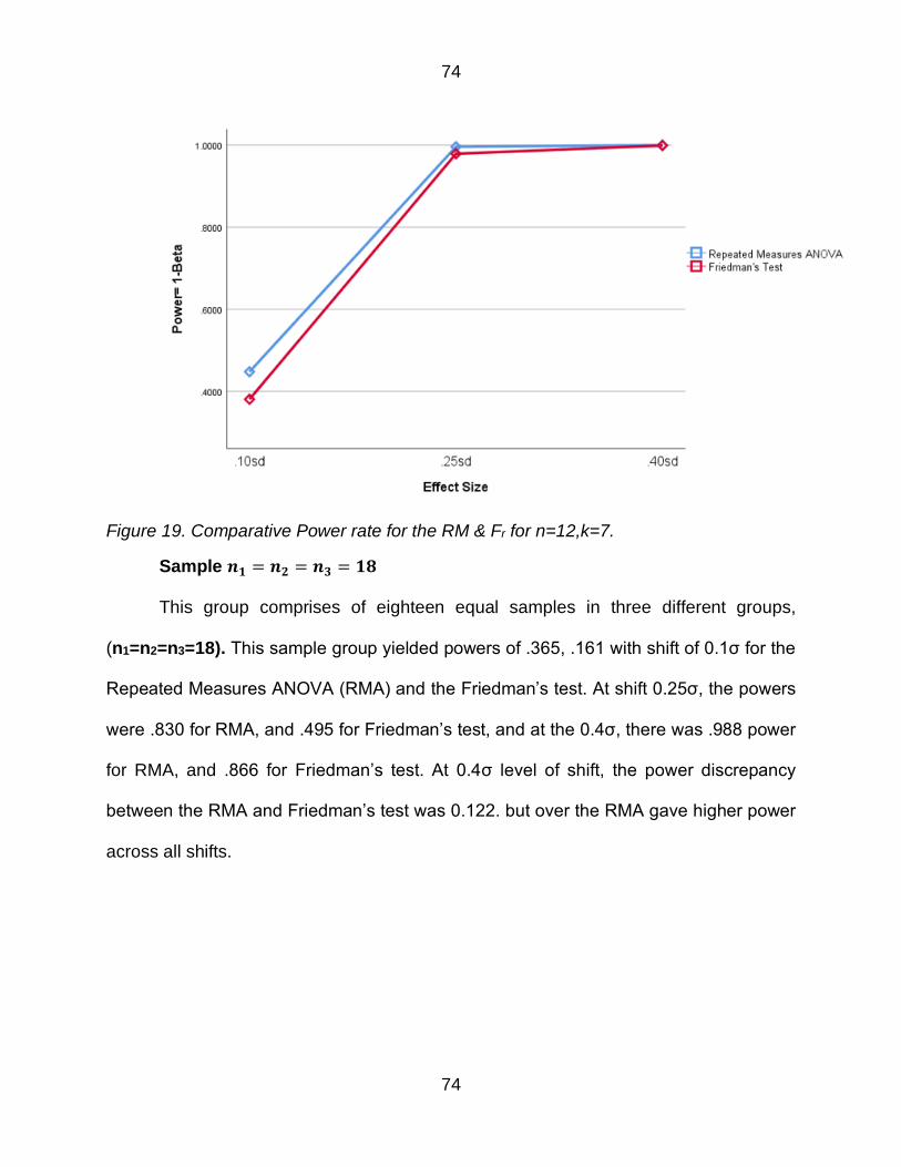
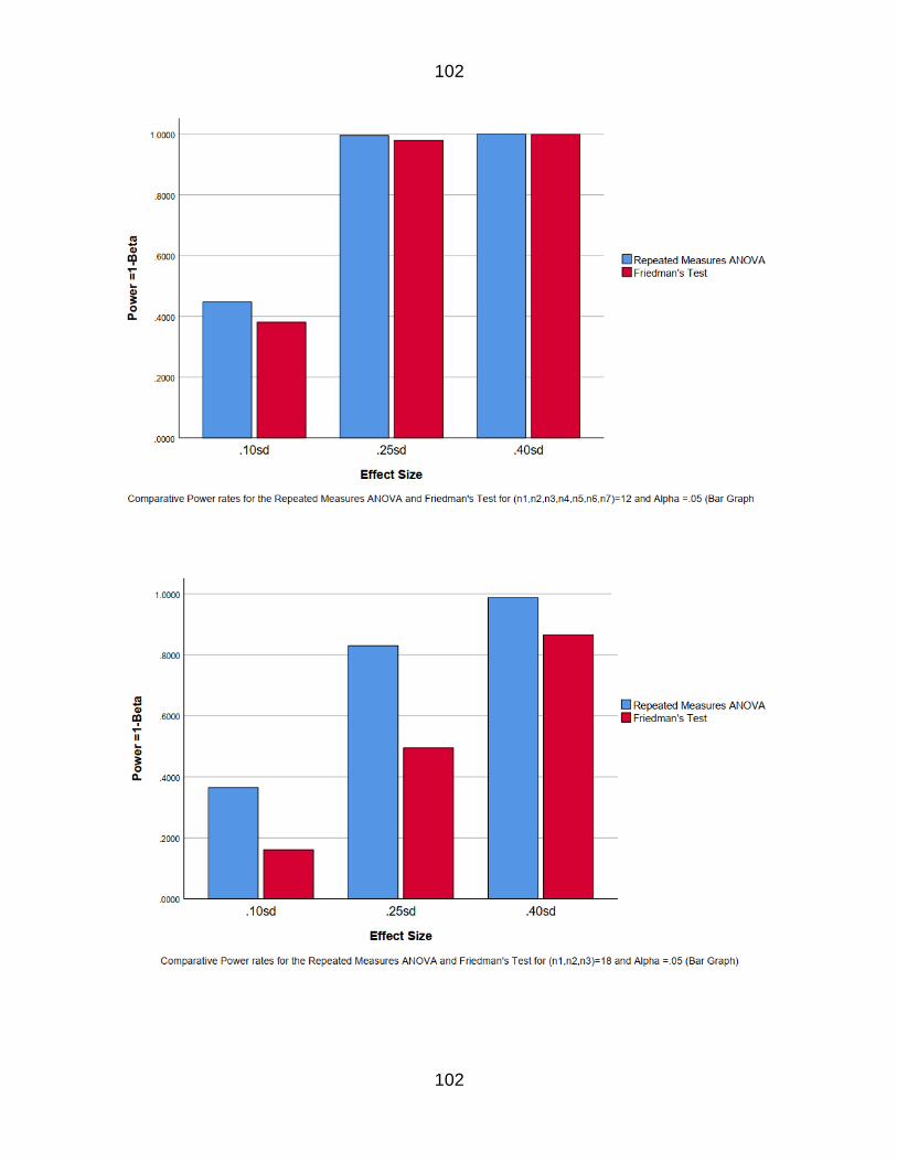
Figure 19 Comparative Power rate for the RM amp Fr for n=12k=7 74
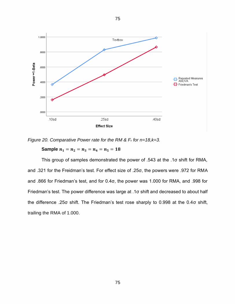
Figure 20 Comparative Power rate for the RM amp Fr for n=18k=3 75
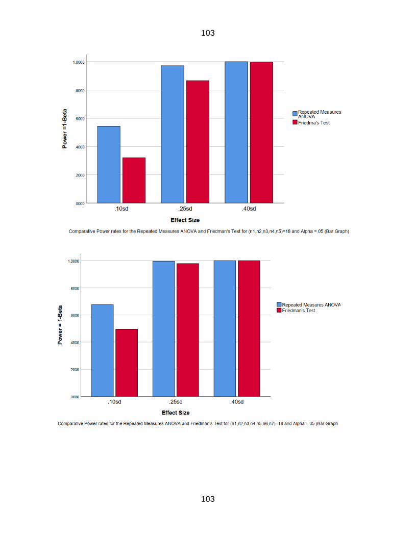
Figure 21 Comparative Power rate for the RM amp Fr for n=18k=5 76
viii
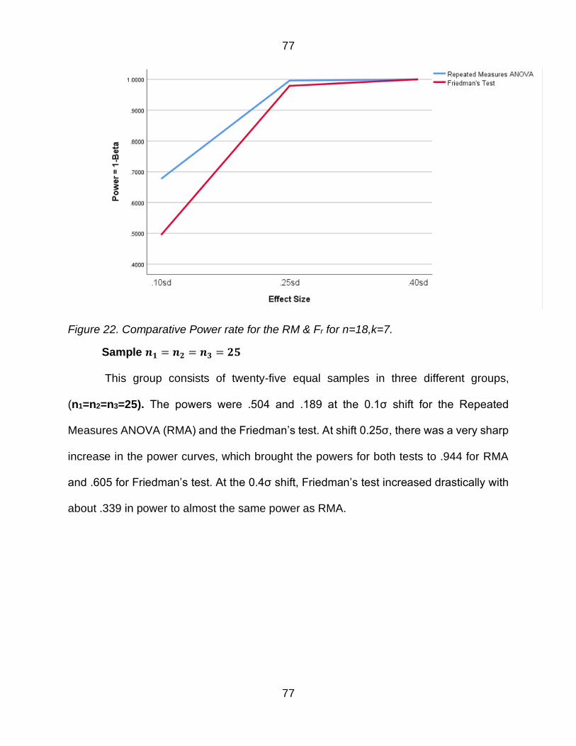
Figure 22 Comparative Power rate for the RM amp Fr for n=18k=7 77
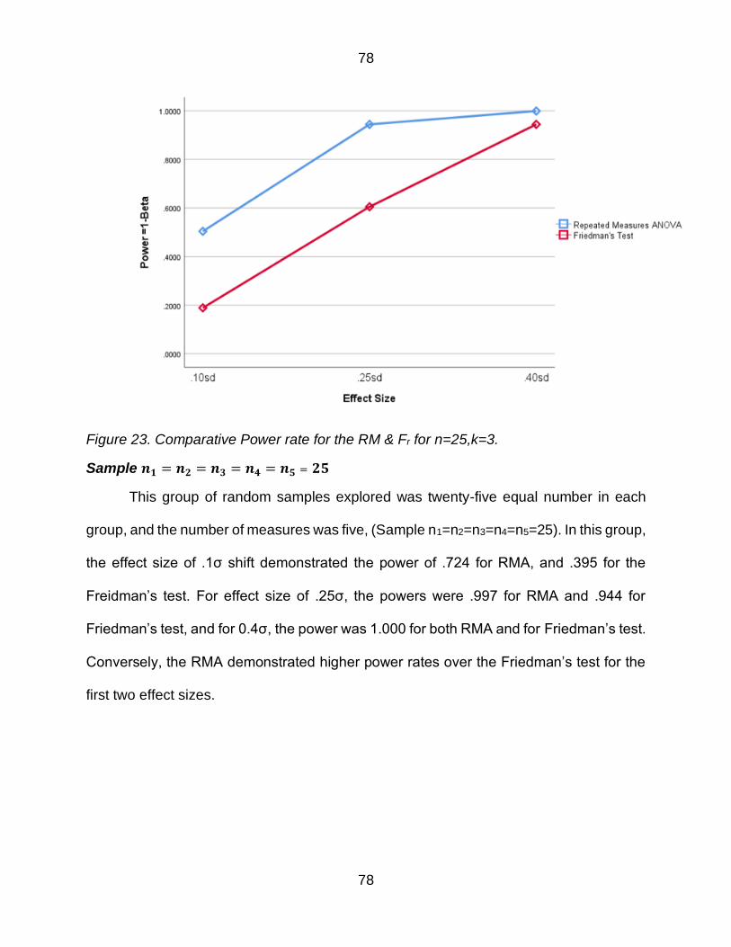
Figure 23 Comparative Power rate for the RM amp Fr for n=25k=3 78
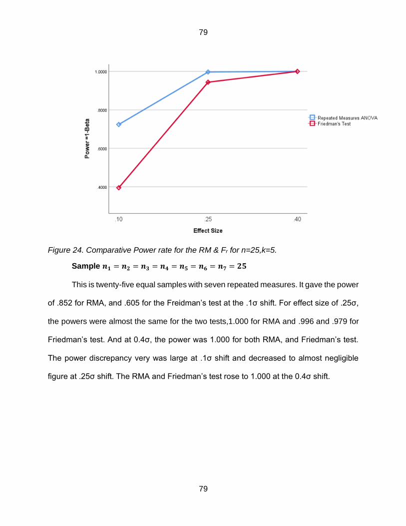
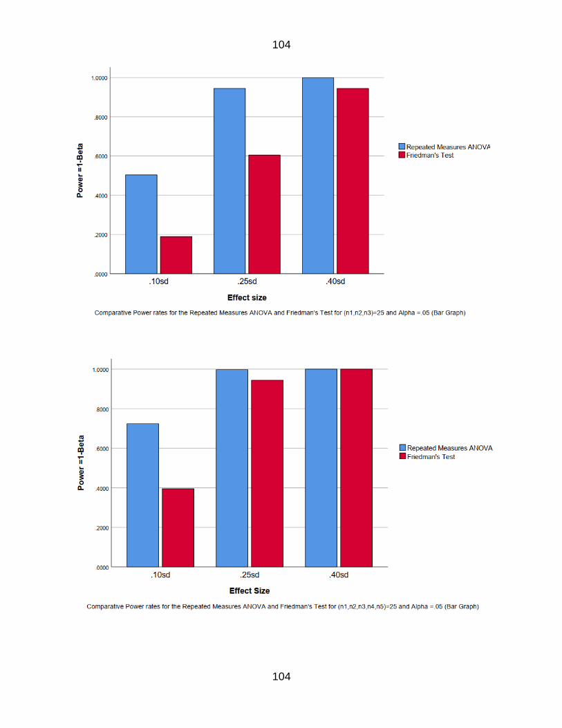
Figure 24 Comparative Power rate for the RM amp Fr for n=25k=5 79
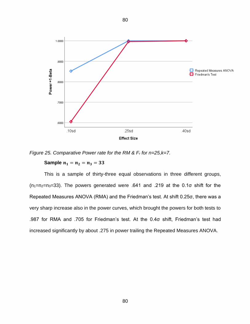
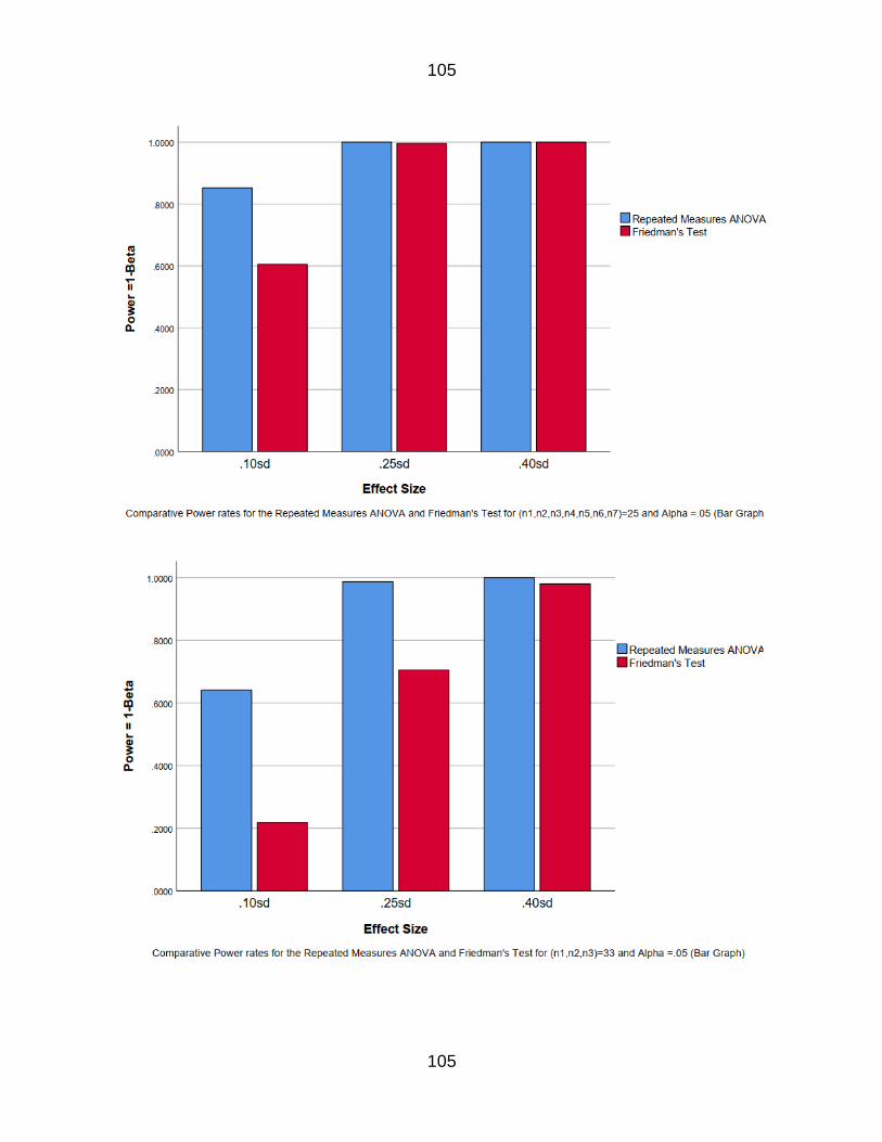
Figure 25 Comparative Power rate for the RM amp Fr for n=25k=7 80
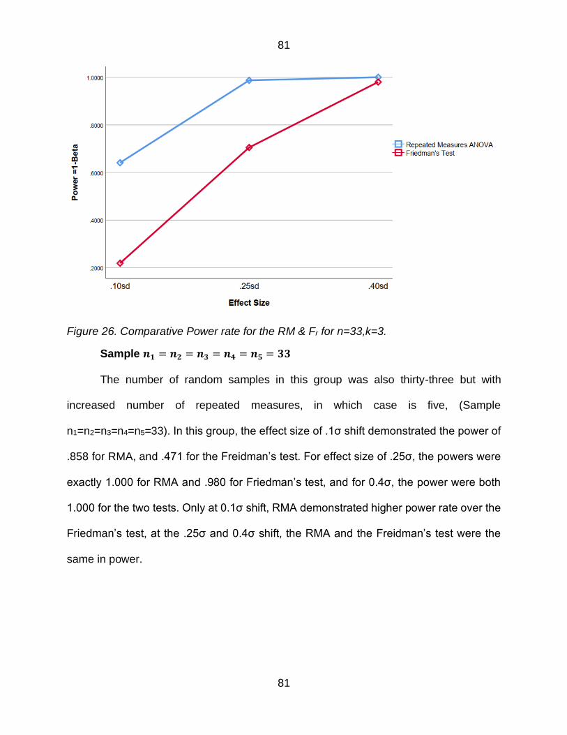
Figure 26 Comparative Power rate for the RM amp Fr for n=33k=3 81
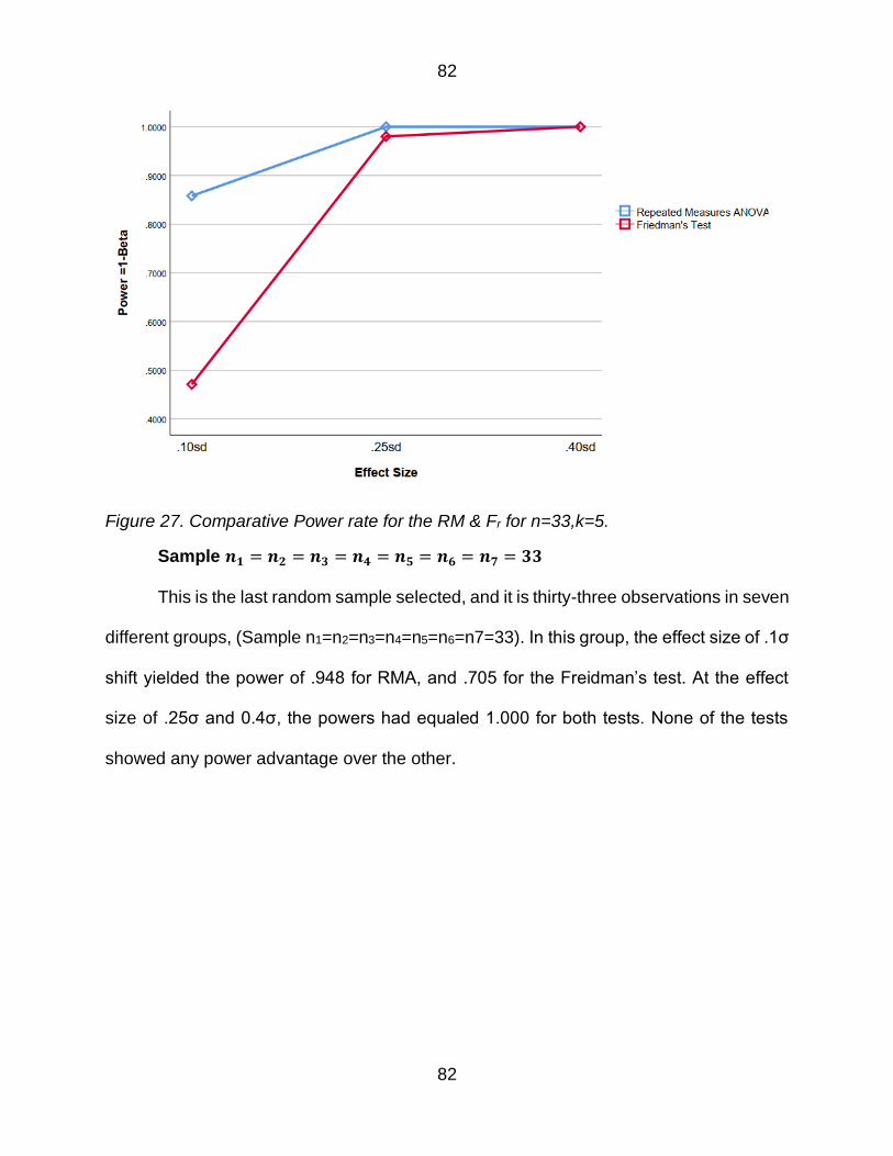
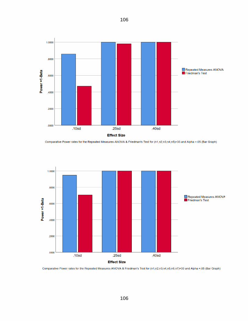
Figure 27 Comparative Power rate for the RM amp Fr for n=33k=5 82
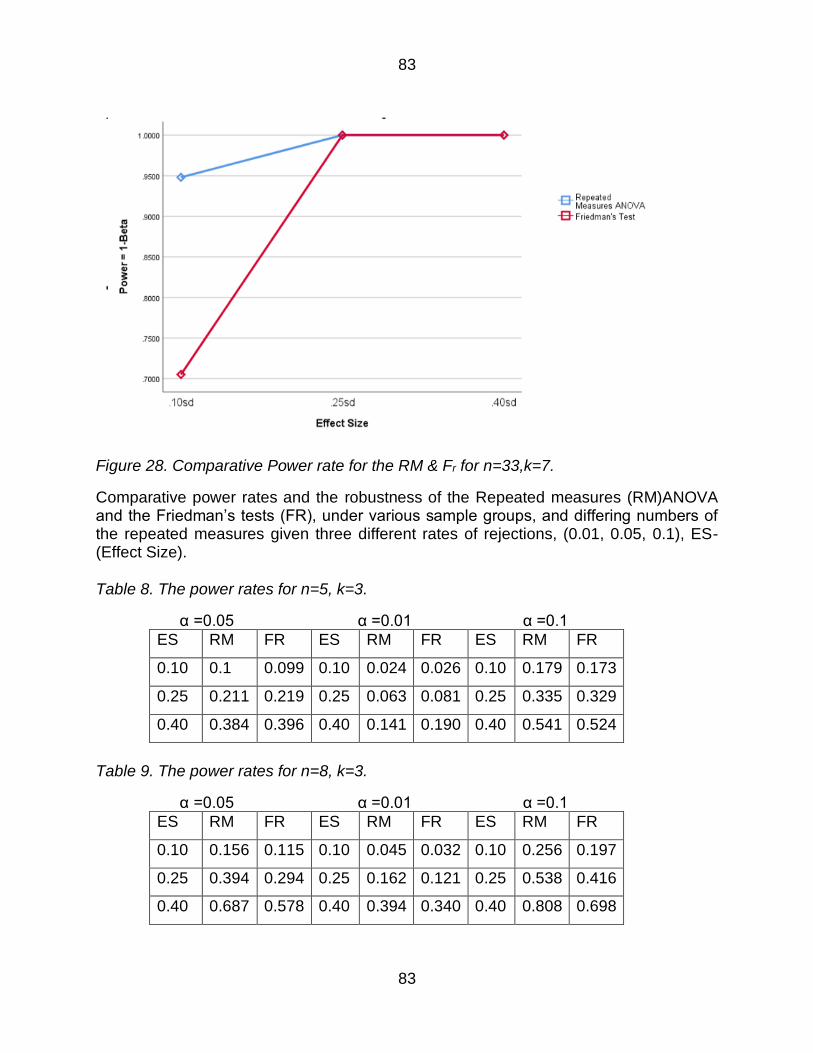
Figure 28 Comparative Power rate for the RM amp Fr for n=33k=7 83
ix
copy COPYRIGHT BY
OPEOLUWA BOLU FADEYI
2021
All Rights Reserved
1
1
CHAPTER ONE
INTRODUCTION
OVERVIEW OF THE PARAMETRIC TESTS
Parametric tests are those which based the necessary assumptions on the
parameters of the underlying population distribution from which the samples are drawn
It is generally believed that parametric tests are robust to the violation of some of the
assumptions this means that the tests have the power to control the probability of
rejecting the false null hypothesis For example ANOVA can be used to analyze ordinal
scale data such as Likert scales even without any consequences (Leys amp Schumann
2010 Nanna amp Sawilowsky 1998 Zimmerman amp Zumbo 1993) Another peculiar
characteristic of a parametric test is that it is uniformly most powerful unbiased (UMPU)
ldquoThis means that when all underlying assumptions are met based on the inference from
the samples no other test has greater ability to detect a true difference for a given samplerdquo
(Bridge amp Sawilowsky 1999 p 229) For example the t-test is uniformly most powerful
unbiased when the assumptions of independence homoscedasticity and normality are
met (Bradley 1968b Kelley amp Sawilowsky 1997) However a ldquolight shiftrdquo in the shapes
of the distribution of the variables when the number of samples in each treatment group
gets close to 30 or more still generates robust results (Glass Peckham amp Sanders 1972
Leys amp Schumann 2010 Lix Keselman amp Keselman 1996 Lumley Diehr Emerson amp
Chen 2002) Studies have been carried out to examine the violation of the assumption
of homogeneity of variances which may have a severe impact on the type I error rate of
F-tests and It has been established that F-test will yield statistically significant results
when the group sample sizes are equal and size of the groups greater than seven (Box
2
2
1954 David amp Johnson 1951 Horsnell 1953 Hsu 1938 Linquist 1953 Norton 1952
Scheffeacute 1959) Another procedure that can be performed when there is the heterogeneity
of variance is to transform or change the form of the data involved Examples of this
procedure are Log transformation square root transformation or inverse transformation
(Blanca Alarcoacuten Arnau Bono amp Bendayan 2017 Keppel 1991 Leys amp Schumann
2010 Lix Keselman amp Keselman 1996 Saste Sananse amp Sonar 2016) This
procedure works well in stabilizing the variances and improve the normality of the dataset
Parametric tests are used to analyze interval and ratio scale data (Bridge amp Sawilowsky
1999 Shah amp Madden 2004) Other examples of parametric tests are the t-test the Chi-
squared test test-of-goodness of fit analysis of variance or F-test analysis of covariance
multiple linear regression and discriminant function analysis (Weber amp Sawilowsky
2009)
The robustness property in the normal distribution test signifies the ability of a test
to retain its Type I error rate close to its nominal alpha as well as its Type II errors for
data sampled from non-normal distributions at a similar rate as those datasets sampled
from a normal distribution (Bridge amp Sawilowsky 1999 Hunter amp May 1993) However
parametric tests are not always tolerant to extreme violations of their underlying
assumptions Outliers are the major causes of shifts in the shapes of the distribution
Outliers can render the results of the parametric tests inaccurate and misleading by
inflating or deflating the error rates This problem of error inflation is made worse by how
frequent outliers are present in a group of scores (Geary 1947 Hunter amp May 1993
Micceri 1989 Nunnally 1978 Pearson 1895 Pearson amp Please 1975 Sawilowsky amp
Blair 1992 Tan 1982) When the assumption of normality is not met ANOVA loses its
3
3
distinct ability of being uniformly most powerful unbiased (UMPU) test as does the t-test
(Sawilowsky 1990 p 100) This emphasizes the importance of rank-based
nonparametric alternative approaches specifically concerning the treatment models of
shift in location parameter The alternative solutions to the problem of severe violation of
underlying assumptions in parametric tests are nonparametric tests robust procedures
data transformation resampling simulations and bootstrapping etc (Feys 2016)
Origin of Nonparametric Tests
Nonparametric tests are distribution-free tests that do not base their requirements
on fulfilling the assumptions of their parent distributions such as F-test or Chi-square
distribution (Kruskal amp Wallis 1952) Such assumptions include normality and
independence of observation Meanwhile there are other assumptions of the
nonparametric tests that are generally considered weak because they are not connected
to the validity of the nonparametric testsrsquo results The assumption could be ignored since
they do not interfere with the functionality of the tests Such assumptions relating to the
population distributions from which they are drawn are generally weak Those
assumptions are not restrictive for the results to be valid (Gibbons 2003) There are three
main types of nonparametric tests namely categorical sign and rank-based tests
(Gleason 2013 Sawilowsky 1990) Nonparametric tests are usually robust to nonnull
distribution and are good alternatives to handling the occurrence of outliers in statistical
analysis Many studies have been carried out on comparing the robustness and the
comparative power advantages of the parametric tests with their nonparametric
counterparts In the two-group layout it is assumed that the data are independently and
identically distributed (IID) Sign test Wilcoxon-Sign Rank test (WSR) and Manny-
4
4
Whitney tests are some of the examples in this group These tests are competitors with
the student t-test paired sample t-test and the independent t-test However when the
number of groups is increased to 3 or more (i e k ge 3) the Kruskal-Wallis test competes
well with the regular one-way ANOVA while Friedmanrsquos test can be applied as an
alternative to the one-way repeated measures ANOVA (Friedman 1937) One of the
assumptions of the Friedman test is that ldquosamples are dependent under all levelsrdquo (Ingram
amp Monks 1992 p 827)
Historically nonparametric tests were viewed as being useful only when the
assumptions of the parametric tests were not met (Lehmann 1975 Marascuilo amp
McSweeney 1977) Subsequently it was proved that when testing for the differences in
location parameters if the distribution shapes are not normal or are heavy-tailed the
nonparametric tests are robust and present considerable power advantages over their
parametric counterparts (Blair amp Higgins 1985 Sawilowsky 1990)
Nonparametric statistics were popular in the 1950s but began to wane for three
reasons in the 1970s Those three reasons were summarized by (Sawilowsky 1990 p
92) (Boneau 1960 Box 1954 Glass Peckham amp Sanders 1972 Linquist 1953)
First it is usually asserted that parametric statistics are extremely robust with respect to the assumption of population normality (Boneau 1960 Box 1954 Glass Peckham amp Sanders 1972 Linquist 1953) precluding the need to consider alternative tests Second it is assumed that nonparametric tests are less powerful than their parametric counterparts (Kerlinger 1964 1973 Nunnally 1975) apparently regardless of the shape of the population from which the data were sampled Third there has been a paucity of nonparametric tests for the more complicated research designs (Bradley 1968)
One of the goals of performing a statistical test is to investigate some claims using
samples and make inferences about the general populations from which the samples are
5
5
drawn Therefore researchers need to understand the criteria for making the right choice
of tests that will yield accurate and clear results for decision-making purposes The
statistical power of a test will determine if such a test carries the ability to detect a
significant statistical effect when such an effect is present The significant level at which
a test will commit a false rejection is called Type I error denoted by the Greek small letter
Alpha (α) A default value of 005 is commonly used in research
Statistical power
Statistical power efficiency refers to the minimum size of the samples required to
determine whether there is an effect due to an intervention This is the ability to reliably
differentiate between the null and the alternative hypothesis of interest To measure the
statistical power of a test effectively Relative Efficiency (RE) and the Asymptotic Relative
Efficiency (ARE) will be considered The relative efficiency of a statistical test is the index
that measures the power of a test by comparing the sample size required of one
parametric test to the sample size of its nonparametric counterpart To achieve an
unbiased estimate the two tests must be subjected to equal conditions that is the
significant level and the hypothesis under which they are both compared must be equal
(Sawilowsky 1990)
Asymptotic Relative Efficiency (ARE) of a statistical test for both parametric and
nonparametric tests is the ratio of two tests as compared to 1 when the sample sizes are
large and the treatment effect is very small Thus if the ARE of a parametric test over the
nonparametric alternative is greater than 1 the parametric test has a power advantage
over its nonparametric counterpart (Pitman 1948 Sawilowsky1990) The ARE is also
called the Pitman efficiency test
6
6
The parametric test that employs the analysis of a complete block design when
comparing only two group means or treatments is the paired t-test The two
nonparametric alternatives in the same category are the Wilcoxon signed ranks (WSR)
test and the sign test The sign test uses the information based on the within-block
rankings to assign ranks to the absolute values of observations when the number of the
groups is 2 (k = 2) Friedmanrsquos test design has extended the procedure of the sign test
to a randomized block design involving more than two comparisons (k ge 3) Therefore
the Friedman test is considered an extension or generalization of the sign test (Hodges
amp Lehmann 1960 Iman Hora amp Conover 1984 Zimmerman amp Zumbo 1993)
Observations generated by subjecting the same set of participants to three or more
different conditions are termed repeated measures or the within-subjects data The
parametric statistical design that is used to analyze this type of observation is the usual
F-test for block data or the One-Way Repeated Measures ANOVA ldquoThe ARE of the
Friedman test as compared to the F test is (3π)k(k + 1) for normal distributions and
[ge864k(k+1)] for other distributionsrdquo (Hager 2007 Iman Hora amp Conover 1984 Potvin
amp Roff 1993 Sen 1967 1968 Zimmerman amp Zumbo 1993)
ldquoThe ARE of a test is related to large sample sizes and very insignificant treatment
effects this is highly impractical in the real-world experiment However Monte Carlo
simulations have been confirmed to play very significant role in calculating the ARE and
RE for small sample sizesrdquo (Sawilowsky 1990 p 93 see also Potvin amp Roff 1993
Zimmerman amp Zumbo 1993)
7
7
Problem of the Study
Several Monte Carlo studies were conducted on the comparative power of the
univariate repeated measures ANOVA and the Friedman test (Hager 2007 Hodges amp
Lehmann 1960 Iman Hora amp Conover 1984 Mack amp Skillings 1980 Potvin amp Roff
1993 Zimmerman amp Zumbo 1993) However conclusions based on simulated data were
limited to data sampled from specific distributions This is a disadvantage in the ability to
generalize the results to the population from which samples were drawn Real-life data
have been found to deviate from the normality assumptions more drastically than those
patterns found in the mathematical distributions (Blanca Arnau Lόpez-Montiel Bono amp
Bendayan 2013 Harvey amp Siddique 2000 Kobayashi 2005 Micceri 1989 Ruscio amp
Roche 2012 Van Der Linder 2006) As a case in point most of what is known regarding
the comparative statistical power of the one-way repeated measures ANOVA and the
Friedman tests were tied to specific mathematical distributions and it is not well known
how the two tests compare with common real-world data
Purpose of this study
The results from previous research have shown that the parametric statistics have
a little power advantage over their nonparametric alternatives when the assumption of
normality holds However under varying non-symmetric distributions the nonparametric
tests yielded comparable power advantages over the parameter-based tests It is
therefore the goal of this study to examine the robustness and comparative statistical
power properties of the one-way repeated measure ANOVA to its nonparametric
counterpart Friedmanrsquos test to the violations of normality using the real-world data which
has not been extensively studied
8
8
Research questions
The research questions addressed in this study are as follows
Will the results of previous simulation studies about the power advantage of
parametric over nonparametric be generalizable to real-world situations
Which of these tests will yield a comparative power advantage under varying
distribution conditions
Relevance to Education and Psychology
Research helps to make inferences about the general population through the
samples drawn from them The tool for reaching this goal is statistical analysis To
generate accurate conclusions and avoid misleading decisions necessity is laid on the
researchers to choose the statistical tools that have appropriate Type I error properties
and comparative statistical power in real-life situations Studies have shown that the
nonparametric statistics have greater power advantages both in the normal distribution
models and the skewed and kurtosis characterized distributions
Limitations of the study
The study is limited to the one-way repeated measures layouts and did not
consider the higher-order procedures that include interactions The treatment alternatives
were restricted to shift in location for various sample sizes and measure combinations
This research work uses the real-life data (mortality count from the COVID-19 data) and
it is analyzed using the SPSS 2601 and GPower for the calculation of the power analysis
as a function of the shift in the location parameter Therefore it is assumed that the results
are replicable under these situations
9
9
Definitions of Terms
Robustness
Hunter and May (1993) defined the robustness of a test as ldquothe extent to which
violation of its assumptions does not significantly affect or change the probability of its
Type 1 errorrdquo (p 386) Sawilowsky (1990) stated ldquothe robustness issue is related not only
to Type 1 error but also to Type II error the compliment of the power of a statistical testrdquo
(p 98)
Power
Bradley (1968) wrote ldquothe power of a test is the probability of itrsquos rejecting a
specified false null hypothesisrdquo (p 56) Power is calculated as 1-β where β signifies the
Type II error (Cohen 1988) As β increases the power of a test decreases
Power Efficiency
Power efficiency is defined as the least sample size needed to notice a true
treatment difference or to identify the false null hypothesis (Sawilowsky 1990)
Interaction
Interaction is present when the pattern of differences associated with either one of
the independent variables changes as a function of the levels of the other independent
variable (Kelley 1994)
Asymptotic Relative Efficiency (ARE)
The Asymptotic Relative Efficiency (also known as Pitman Efficiency) compares
the relative efficiency of two statistical tests with large samples and small treatment
effects (Sawilowsky 1990) Blair and Higgins (1985) defined ARE as the ldquolimiting value
of ba as ldquoardquo is allowed to vary in such a way as to give test A the same power as test B
10
10
while ldquobrdquo approaches infinity and the treatment effect approaches zerordquo (p 120) This
means that the efficiency of the competing nonparametric statistic is divided by that of the
parametric statistic If the ratio is found to be less than one the nonparametric test is
predicted to be less powerful than the parametric counterpart (Kelley 1994)
Type I Error
This is when the result of a statistical test shows that there is an effect in the
treatment when there is none the decision to reject the null hypothesis is made It is
denoted by the Greek small letter alpha (α)
Type II Error
The decision of a test to fail to reject a null hypothesis (there is no treatment effect)
when it is false is known as the Type II error It is called beta (β)
11
11
CHAPTER TWO
THEORETICAL FOUNDATIONS AND LITERATURE REVIEW
Introduction
Researchers and organizations are often faced with the decision of choosing an
intervention that yields a better result from between two conditions or treatments The T-
test is the statistical tool that has been very effective in solving this problem However
this tool is not relevant in situations of choosing the most effective intervention among
groups that are more than two In that case the perfect substitute to the t-test is the
Analysis of Variance (ANOVA) ldquoAnalysis of variance may be defined as a technique
whereby the total variation present in a set of data is partitioned into two or more
components Associated with each of these components is a specific source of variations
so that in the analysis it is possible to ascertain the magnitude of the contributions of each
of these sources to the total variationrdquo (Daniel 2009 p 306) ANOVA model is an
extension of the t-test therefore it can fit into many different statistical designs based on
the numbers of factors and levels Factors are independent variables that can affect some
outcomes of interest Levels are those specific values attached to factors ANOVA models
test the hypotheses about population means and population variances Invariably it
analyzes variances to make conclusions about the population means (Methods 2020
Lane 2019)
ANOVA is divided into different groups based on the different types of experimental
designs for example one-way designs mixed factor or mixed-method designs repeated
measures ANOVA and two-way ANOVA etc This research work focused on comparing
the robustness and power of Repeated Measures ANOVA with its nonparametric
12
12
counterpart- the Friedman test and how each test behaves with the real-world dataset
Higher-order designs that involve interactions are not covered in this research study
ANOVA was developed by Sir Ronald Fisher in 1918 (Stevens 1999) It is an
analytical tool used in statistics that splits the total variance in a dataset into two parts
1 Systematic factors or errors and 2 Random factors or errors Error is not a mistake
but a part of the measuring process It is called observational or experimental error
Random errors are statistical alterations (in either direction) in the measured data
due to the characteristics of different measurements These errors are due to the peculiar
attributes of different participants in the experiment Random error in a statistical sense
is defined in terms of mean error the correlation between the error and true scores where
the correlation between errors is assumed to be zero The direction of these types of
errors is not predictable in an experiment and its distribution usually follows a normal
distribution Random errors do not have a statistical impact on the dataset only the last
significant digit of a measurement is altered Random errors can be eliminated by
increasing the number of samples taken and taking the average value of the sample sizes
Systematic errors follow a single direction multiple times due to factors that
interfere with the instrument used in generating data Systematic errors have a statistical
impact on the results of the given experiment For example if an experimenter wants to
know the effects of two teaching methods on the results of students in different classes
one class was well lit and the other poorly lit The means (averages) of these two classes
will be statistically different because the two studies are not conducted under the same
environmental conditions Therefore the system is biased Systematic errors can occur
due to faulty human interpretations change in the environment during the experiments
13
13
(Khillar 2020) Researchers can control for this type of error by randomization or blocking
technique by using proper techniques calibrating equipment and employing standards
etc Unlike the random errors systematic errors cannot be analyzed by generating a
mean value for the samples because these types of errors are reproduced each time a
similar study is conducted Invariably this type of error can be more dangerous and the
results generated from this type of observation will lead to inaccurate decisions
ANOVA is used to determine the effects of the independent variables on the
dependent variables in an experiment Some assumptions need to be verified before
ANOVA can be an appropriate tool for analysis
bull Homogeneity of the variance of each group of the dataset
bull The observations data groups are independent of each other
bull The data set is normally distributed on the dependent variable
The F-test is conceptualized as a ratio of systematic error to random error Ie
Variance Ratio is another name for F-test
119865 = 119872119878119879
119872119878119864 asymp
119904119910119904119905119890119898119886119905119894119888 119890119903119903119900119903
119903119886119899119889119900119898 119890119903119903119900119903 (1)
where MST is Mean Square Total and MSE is Mean Square Error F is equal to the
mean square total divided by the mean square error which is equivalent to the systematic
error divided by the random error F-values range from 0 to positive infinity (0 to +infin) and
it depends on a pair of degrees of freedom (df) ie df for the numerator and df for the
denominator The ANOVA F-test allows the comparison of 3 or more groups of
observations to determine the between sample errors and within samples errors
14
14
This was not possible with the two-sample group t-test In ANOVA there are two
types of hypotheses in the Neyman-Pearson frequentist approach to experiments which
includes the null and alternative hypotheses The null hypothesis denoted by Ho
indicates that there is no statistically significant difference in the group means while the
alternative hypothesis (Ha) is the exact opposite of the claim stated in the null hypothesis
The hypothesis tested in one-way ANOVA is Ho micro1 = micro2 = hellip micro119899 which seeks to
determine if there are differences among at least one of the sample means as opposed
to whether such differences are due to sampling error (Chan amp Walmsley 1997) The
ANOVA is relatively robust to departures from population normality when testing for a shift
in location (Hecke 2010) However in situations where the normality assumption is
violated the nonparametric alternatives which are completely robust offer additional
power in detecting a false null hypothesis Rank-based nonparametric alternatives employ
a ranking technique to convert the original data into ranks
There are divergent views concerning information integrity when data are ranked
Some researchers opined data converted into ranks results in the loss of information and
less powerful test (Adams amp Anthony 1996 Borg 1987 Chase 1976 Garrett 1966
Gravetter amp Wallanu 1985 Kerlinger 1964) Wolfowitz (1949) asserted ldquothe only kind of
information a nonparametric procedure is likely to waste is information that is unavailable
anywayrdquo (p 175) Others affirmed that the ranking of scores removes noise and increases
the statistical power of a test (Blair Higgins amp Smitley 1980 Blair amp Higgins 1985
Langhehn Berger Higgins Blair amp Mallows 2000 Sawilowsky 1993) Transformation
techniques are typically performed in order to stabilize error variance improve normality
of the datasets and simplify the model (Saste Sananse amp Sonar 2016 p 654)
15
15
Solomon amp Sawilowsky (2009) also note ldquorank-based transformations not only attempt to
equate the means and homogenize the variance of test-score distributions they also aim
to create conformity in the third and fourth moments skewness and kurtosisrdquo (p 449)
Repeated Measures ANOVA
Repeated measures ANOVA is a technique of analyzing the mean differences that
exist among groups of observations when the number of subjects is few changes in
participantsrsquo behavior (variable) need to be measured over long periods This model
subjects the same group of participants multiple times to different conditions or
interventions to see how they perform at different times and also if there are noticeable
improvements beyond those due to chance Improvements or changes in the
performance of the subjects can either be in the positive or negative direction For
example when a group of obese women is randomly assigned into 3 different diet plans
to monitor the effect on their body weight for 4-weeks the improvement is expected to be
in the negative direction (to lose some body fat) However when a group of cancer
patients is given three different brands of medication the expected change will be in the
positive direction (good health) When the same group of individuals is repeatedly
assessed over a specific period it is called the within-subject or (RM) Repeated Measures
ANOVA (Stevens 1999) Repeated measures ANOVA is termed the within-subject
measures because researchers compare the means of the varying observations from the
same subject each subject representing a block and provides control values against
which to compare The repeated observations which are taken from the same subject
tend to be dependent among each other Since repeated scores are highly correlated
among groups it takes very little variation in the treatment means to detect any effect that
16
16
is present This makes the within-subject design possess more power advantage over the
between-subjects designs However when different participants are exposed to the same
level of treatments then the situation is the between-subject design also variabilities
among participants are present The within-subject ANOVA has a greater power
advantage over the between-subject design because the random error is reduced
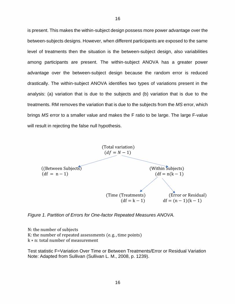
drastically The within-subject ANOVA identifies two types of variations present in the
analysis (a) variation that is due to the subjects and (b) variation that is due to the
treatments RM removes the variation that is due to the subjects from the MS error which
brings MS error to a smaller value and makes the F ratio to be large The large F-value
will result in rejecting the false null hypothesis
(Total variation)
(119889119891 = 119873 minus 1)
((Between Subjects) (Within Subjects)
(df = n minus 1) (df = n(k minus 1) (Time (Treatments) (Error or Residual) (df = k minus 1) df = (n minus 1)(k minus 1)
Figure 1 Partition of Errors for One-factor Repeated Measures ANOVA
N the number of subjects K the number of repeated assessments (e g time points) k lowast n total number of measurement Test statistic F=Variation Over Time or Between TreatmentsError or Residual Variation Note Adapted from Sullivan (Sullivan L M 2008 p 1239)
17
17
Randomized Block Design
In a randomized block design each subject serves as a block and their responses
serve as different conditions This design eliminates the equivalency problem before the
interventions and removes participant variability from the error term By that fewer
participants can be tested at all levels of the experiment making each subject serve as its
own control against which to compare the other variables This technique is best
appreciated in the medical world where large numbers of participants are not accessible
Repeated measures design could also have some shortcomings These may include
bull the carryover effect when the residue of the first treatment affects the
experimental outcomes
bull the latency effect is the effect that is present but did not manifest until the
subsequent treatments are administered and
bull fatigue is because of the stress participants experienced by involving in series of
experiments which can affect the result of subsequent interventions (Girden 1992
Stevens 1999)
When a researcher faces a situation of exposing the same subjects to several
treatments at a time caution needs to be taken in the order of administering the
treatments The counterbalancing procedure of administering the treatments was
proposed by Girden (1992) to alleviate the problem of treatment ordering effect For
example ldquoCarry-over effect can be minimized by lengthening the time between
treatments latency however is harder to controlrdquo (p3) Also holding the extraneous
variable constant can help reduce some of the latency effects administering short and
interesting (activities) conditions can eliminate fatigue in the participants during the
18
18
experimental process However when any of the effects due to the patterns of
treatments influence the outcomes of the experiment there are threats to the internal
validity of the test Some factors that pose threats to the internal validity of RM are
listed below
ldquoRegression threat (when subjects are tested several times their scores tend to
regress towards the means) a maturation threat (subjects may change during the
course of the experiment) and a history threat (events outside the experiment that may
change the response of subjects between the repeated measures)rdquo (Lumen Boundless
2020)
Statistical analyses always have some assumptions to be met before their
applications can be valid Of no exception is the repeated measures ANOVA
The univariate assumptions of the repeated measures ANOVA are listed below
I The dependent variables of each level of the factor must follow a multivariate
normal distribution pattern
II the variances of the difference scores between each level of factor must be equal
across levels
III correlations between any pair of the levels must be the same across levels eg
ρ(L1 L2) = (L2 L3) = (L1 L3) (II amp III constitute circularity or sphericity
assumption)
IV subject scores should be independent of each other
V Participants must be randomly sampled
19
19
Parametric and Nonparametric Tests
The term parameter is generally used to categorize unknown features of the
population A parameter is often an unspecified constant appearing in a family of
probability distributions but the word can also be interpreted in a broader sense to include
almost all descriptions of populations characteristics within a family (Gibbons 2003 p
1) In a distribution-free inference either hypothesis testing or estimation the methods of
testing are based on sampled data whose underlying distributions are completely different
from distributions of the population from which the samples were drawn Therefore the
assumptions about the parent distribution are not needed (Gibbons 2003)
Nonparametric test connotes the claim of the hypothesis test which has nothing to do with
parameter values ldquoNonparametric statistic is defined as the treatment of either
nonparametric types of inferences or analogies to standard statistical problems when
specific distribution assumptions are replaced by very general assumptions and the
analysis is based on some function of the sample observations whose sampling
distribution can be determined without knowledge of the specific distribution function of
the underlying population Perhaps the chief advantage of nonparametric tests lies in their
very generality and an assessment of their performance under conditions unrestricted
by and different from the intrinsic postulates in classical tests seems more expedient
(Gibbons 1993 p 4 Gibbons 2003 p 6-7)
Corder amp Foreman (2009) state ldquospecifically parametric assumptions include samples
that
bull are randomly drawn from a normally distributed population
20
20
bull consist of independent observations except for paired values
bull have respective populations of approximately equal variances
bull consist of values on an interval or ratio measurement scale
bull are adequately large and approximately resemble a normal distributionrdquo (p 1-2)
However different researchers have defined the minimum sample size for using a
parametric statistical test differently eg Pett (1997) and Salkind (2004) suggest n gt
30 as common in research while Warner (2008) consider a sample of greater than
twenty (n gt 20) as a minimum and a sample of more than ten (n gt 10) per group as
an absolute minimum
When a dataset does not satisfy any of the above-listed assumptions then violation
occurs In the situation of assumption violations few corrections may be considered
before parametric statistics can be used for such analysis First with detailed
explanations extreme values or occurrences that may shift the distribution shapes can
be eliminated or dropped Second the application of rank transformation techniques can
be used to change the observations from interval or ratio scale to (ranks) ordinal scales
(see Conover amp Iman 1981 for details) Although this method has been seriously
criticized and termed ldquocontroversial methodrdquo (Thompson 1991 p 410 see also Akritas
1991 Blair amp Higgins 1985 Sawilowsky Blair amp Higgins 1989) All the alterations or
modifications must be displayed in the discussion section of the analysis Fortunately
another body of statistical tests has emerged that does not require the form of the dataset
to be changed before analysis These are the Nonparametric Tests (Corder amp Foreman
2009)
21
21
Jacob Wolfowitz first coined the term nonparametric by saying we shall refer to
this situation (where a distribution is completely determined by the knowledge of its finite
parameter set) as the parametric case and denote the opposite case where the
functional forms of a distribution are unknown as the nonparametric case (Wolfowitz
1942 p 264) Hollander amp Wolfe (1999) stated explicitly ldquoin the 60+ years since the origin
of nonparametric statistical methods in the mid-1930s these methods have flourished
and have emerged as the preferred methodology for statisticians and other scientists
doing data analysisrdquo (p xiii)
The drastic success of nonparametric statistics over the era of six years can be
credited to the following merits
bull Nonparametric methods require less and unrestrictive assumptions about the
underlying distributions of the parent populations from which the data are sampled
bull ldquoNonparametric procedures enable the users to obtain exact statistical properties
Eg exact P-values for tests exact coverage probabilities for confidence intervals
exact experimental-wise error rates for multiple comparison procedures and exact
coverage probability for confidence bands even in the face of nonnormalityrdquo
(Siegel 1956 p 32)
bull Nonparametric techniques are somewhat easy to understand and easier to apply
bull Outliers which distort the distribution shapes cannot influence the nonparametric
techniques since score ranks are only needed
bull ldquoNonparametric tests are applicable in many statistical designs where normal
theory models cannot be utilizedrdquo (Hollander amp Wolfe 1999 p 1)
22
22
How Rank Transform Techniques Work
ldquoA problem that applied statisticians have been confronted with virtually since the
inception of parametric statistics is that of fitting real-world problems into the framework
of normal statistical theory when many of the data they deal with are clearly non-normal
From such problems have emerged two distinct approaches or schools of thought (a)
transform the data to a form more closely resembling a normal distribution framework or
(b) use a distribution-free procedurerdquo (Conover and Iman1981 p 124) The application
of rank transform techniques to change the form of data from interval or ratio to ordinal
scales before applying the parametric model for analysis is what Conover (1980)
proposed as the rank transformation (RT) approach He termed this approach as a bridge
between the parametric and nonparametric tests by simply replacing the data with their
ranks then apply the usual parametric tests to the ranks
Research showed that rank-based tests yield a comparable power advantage over
the classical counterparts (Hodges amp Lehmann 1960 Iman Hora and Conover 1984
Sawilowsky 1990) Hajek amp Sidak (1967) stated rank tests are derived from the family of
permutation tests and were developed ldquoto provide exact tests for wide (nonparametric)
hypothesis similar to those developed for parametric models in the small sample theoryrdquo
(p 11) Rank tests ldquomaintain the properties of the parent permutation test in being
nonparametric exact tests and yet these procedures are often easy to computerdquo
(Sawilowsky 1990 p 94)
The ranking of observations carries some merits
bull The methods of calculation are very simple
23
23
bull Only very general assumptions are made about the kind of distributions from which
the observations arise
bull Rank tests have the chance of detecting the kinds of differences of real interest
bull ldquoIf there are multiple samples the mean ranks for any of them are jointly distributed
approximately according to a multivariate normal distribution provided that the
sample sizes are not too smallrdquo (Chan amp Walmsley 1997 p 1757)
bull ldquoRank transformation techniques results in a class of nonparametric methods that
includes the Wilcoxon-Mann-Whitney test Kruskal-Wallis test the Wilcoxon
signed ranks test the Friedman test Spearmanrsquos rho and others It also furnishes
useful methods in multiple regression discriminant analysis cluster analysis
analysis of experimental designs and multiple comparisonsrdquo (Conover amp Iman
1981 p 124)
bull ldquoVariance estimates based on ranks are less sensitive to the values of outliers than
are those based on the original data
bull The use of RT methods protects the practitioner against making the false decisions
than can result from a distorted significance level due to nonnormalityrdquo (Potvin amp
Roff 1993 p 1621)
Methods of Ranking
Four ways of ranking data were suggested by Conover and Iman
bull ldquoRank Transform (RT)1 is when the entire observation is ranked together from
smallest to the largest with the smallest observation having rank 1 second
smallest having rank 2 and so on Average ranks are assigned in case of ties
24
24
bull In RT 2- the observations are partitioned into subsets and each subset is
ranked within itself independently of the other subsets This is the case of the
Friedman test
bull RT 3 ndash this rank transformation is RT-1 applied after some appropriate re-
expression of the data
bull RT 4- the RT-2 type is applied to some appropriate re-expression of the datardquo
(p 124)
Friedman A Nonparametric Alternative to the Repeated Measures ANOVA
Friedmanrsquos ANOVA is a nonparametric test that examines whether more than two
dependent groups mean ranks differ It is the nonparametric version of one-way repeated-
measures ANOVA The Friedman test is perhaps the most popular among the rank tests
for analyzing k-related samples The method of ranking random block data was discussed
in detail by Friedman (1937)
The test statistic for the Friedman test involves grouping observations together
based on their similar characteristics which forms the blocks of data The summary of
the test procedure is as follows
I Arrange the scores in a table that have K columns (conditions or
treatments) and N rows (subjects or groups)
II Rank the variables across the levels of the factor (row) that is from 1 to K
III Determine the sum of the ranks for each level of the factors and divide the
value by the number of the subjects (119929119947
119951) This is termed 119895
25
25
IV Determine the sum of the variables across the levels of the factor (row) that
is from 1 to K multiply this value by half (119870 + 1)21 that is the grand mean
Label this value
V ldquoThe test statistics is a function of the sum of squares of the deviations
between the treatment rank sums 119895 and the grand mean rdquo (Gibbons
1993 p 55)
The formula is written as follows
119878 = sum(119895
119896
119895=1
minus )2 equiv 119878 = sum(119929119947
119951
119896
119895=1
) minus (k + 1
2)2 (2)
119872 = 12119899
119896(119896 + 1)119878 (3)
Where n is the number of rows or subjects k is the number of columns and S is a function
of the sum of squares of the deviations between the treatment rank sums 119895 and the
grand mean Or ldquothe sum of the squares of the deviations of the mean of the ranks of
the columns from the overall mean rankrdquo
An alternate formula that does not use S was the test statistic as proposed by
Friedman and it is as follows
119872 = [12
119899119896(119896+1) sum 119896
119895=1 1198771198952] minus 3119899(119896 + 1) (4)
Where n is the number of rows k is the number of columns and 119895 Is the rank sum
for the Jth column J = 12 3 krdquo (Fahoom amp Sawilowsky 2000 p 26 See also
Pereira Afonso amp Medeiros 2015 Siegel amp Castellan Jr 1988) Note All these statistics
will arrive at the same result ldquoWhen the number of treatments and blocks is large it is
26
26
generally assumed that S with the degree of freedom k-1 tends to be asymptotically
distributed according to the Chi-squared (1199092) approximationrdquo (Siegel1956 p 168)
The model for this test statistic was developed by Friedman (1937) The design assumed
that the additive model holds as follows
119883119894119895 = micro + 120573119894 + 120591119895 + 119864119894119895 (5)
where 119883119894119895 is the value of each treatment (119895119905ℎ) in the (119894119905ℎ) block micro is the grand mean 120591119895is
the (119895119905ℎ) treatment effect β119894 is the (119894119905ℎ) block effect The errors 119864119894119895 are assumed to be
independent and identically distributed (iid) with continuous distribution function F(x)
(Skillings amp Mack 1981 p 171) Friedmans test is an analog to the one-way repeated
measures ANOVA where the same participants are subjected to different treatments or
conditions
Hypothesis Testing and Errors in Statistical Analysis
Statistical inference is in two major forms estimation and hypothesis testing ldquoThe
purpose of hypothesis testing is to aid the clinician researcher or administrator in
reaching a conclusion concerning a population by examining a sample from that
populationrdquo (Daniel 2009 p 216) Hypothesis testing and power go hand in hand In
statistical analysis two hypotheses are highlighted the null hypothesis or the statistical
hypothesis which is the hypothesis of no effect of treatment or intervention or zero
difference among the sample means It contains a statement of equality and its ldquoclaim
may be evaluated by the appropriate statistical techniquerdquo (Daniel 2009 p 217) Then
the alternative hypothesis counters whatever is stated in the null hypothesis it is the
claim that is believed to be true if the statistical results reject the null hypothesis
27
27
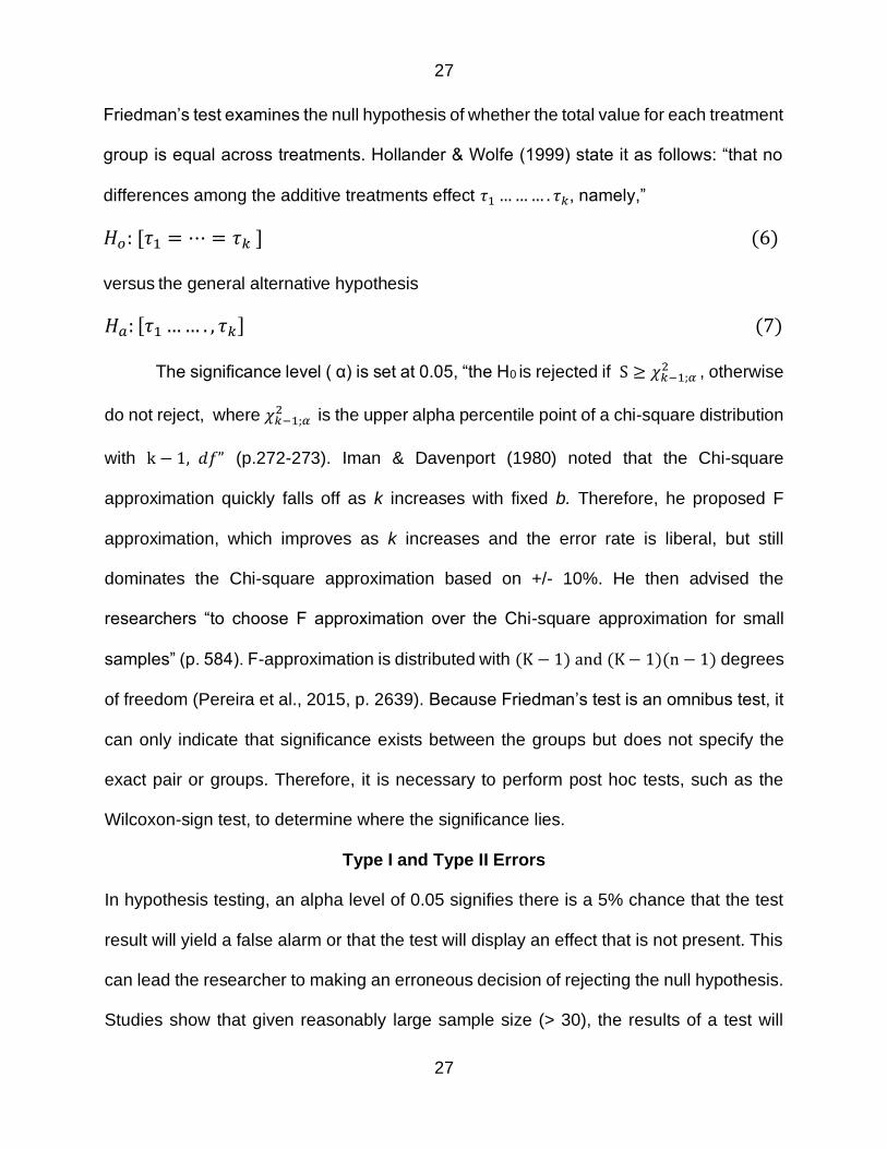
Friedmanrsquos test examines the null hypothesis of whether the total value for each treatment
group is equal across treatments Hollander amp Wolfe (1999) state it as follows ldquothat no
differences among the additive treatments effect 1205911 hellip hellip hellip 120591119896 namelyrdquo
119867119900 [1205911 = ⋯ = 120591119896 ] (6)
versus the general alternative hypothesis
119867119886 [1205911 hellip hellip 120591119896] (7)
The significance level ( α) is set at 005 ldquothe H0 is rejected if S ge 120594119896minus1120572 2 otherwise
do not reject where 120594119896minus1120572 2 is the upper alpha percentile point of a chi-square distribution
with k minus 1 119889119891rdquo (p272-273) Iman amp Davenport (1980) noted that the Chi-square
approximation quickly falls off as k increases with fixed b Therefore he proposed F
approximation which improves as k increases and the error rate is liberal but still
dominates the Chi-square approximation based on +- 10 He then advised the
researchers ldquoto choose F approximation over the Chi-square approximation for small
samplesrdquo (p 584) F-approximation is distributed with (K minus 1) and (K minus 1)(n minus 1) degrees
of freedom (Pereira et al 2015 p 2639) Because Friedmanrsquos test is an omnibus test it
can only indicate that significance exists between the groups but does not specify the
exact pair or groups Therefore it is necessary to perform post hoc tests such as the
Wilcoxon-sign test to determine where the significance lies
Type I and Type II Errors
In hypothesis testing an alpha level of 005 signifies there is a 5 chance that the test
result will yield a false alarm or that the test will display an effect that is not present This
can lead the researcher to making an erroneous decision of rejecting the null hypothesis
Studies show that given reasonably large sample size (gt 30) the results of a test will
28
28
always yield a significant effect even if the effect is due to sampling errors (Akbaryan
2013 Johnson 1995 Kim 2015 Steidl Hayes amp Schauber 1997 Thomas amp Juanes
1996) This is the first type of error (Type I error) in hypothesis testing The second type
of error is the Type II error denoted by β This error is committed when the result of a test
fails to reject the false null hypothesis Then ldquothe power analysis (retrospective or
posteriori power analysis)rdquo of such test needs to be performed in order to provide
explanation and confirmation to the validity of the test resultsrdquo (Steidl Hayes amp Schauber
1997 p 271) To reduce the rate of error alpha can be set at a very small value (stringent
alpha) Beta (β) is directly related to the power of a test Statistical power is the probability
that the result will find a true effect that is present in the analysis and then reject the
false null hypothesis of no difference (Bridge amp Sawilowsky 1999 Cohen 1962 1969
Faul Erdfelder amp Buchner 2007 Kim 2015 Kupzyk 2011 Park amp Schutz 1999 Potvin
1996 Steidl et al 1997 Thomas amp Juanes 1996)
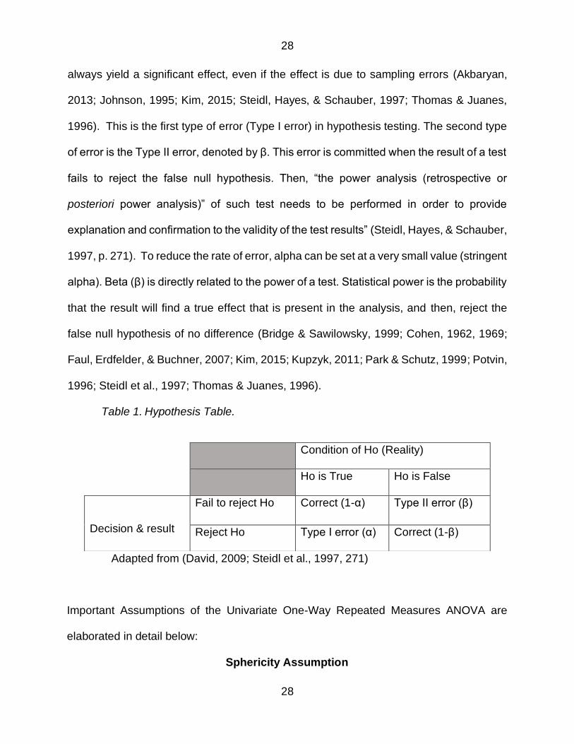
Table 1 Hypothesis Table
Adapted from (David 2009 Steidl et al 1997 271)
Important Assumptions of the Univariate One-Way Repeated Measures ANOVA are
elaborated in detail below
Sphericity Assumption
Condition of Ho (Reality)
Ho is True Ho is False
Decision amp result
Fail to reject Ho Correct (1-α) Type II error (β)
Reject Ho Type I error (α) Correct (1-β)
29
29
Before the univariate method of analyzing block-designs can be the appropriate
choice of the test statistic for any observation the degree of variability (variances) within
each level of intervention must be equal Generally there is always some level of
interrelationships among observations scores are dependent on each other Therefore
it is assumed that the variances of the differences (covariances) between each pair of the
variables of within-factor level must be equal across treatments These two patterns of
variabilities are called compound symmetry (Box 1954) and are later termed sphericity
or circularity assumption (Huynh amp Feldt 1970) Sphericity is equivalent to the
homogeneity of variance assumption in the between factor or independent measures
ANOVA For the two-sample t-test the assumption of homogeneity of variances is always
a work-over since there is only one covariance present Invariably covariance is the
deviations from the mean of each of two measures for each person this connotes that
the means and the variances of the differences can be obtained by subtracting the first
observation from the second observation and the result must be the same for the
difference between the first observation and third observation Simply put ldquosphericity
requires that variances of differences for all treatment combinations be homogeneous ie
1205901199101minus11991022 = 1205901199102
2 minus 1199103 119890119905119888rdquo (Girden 1992 p16 Lamb 2003 p 14) Therefore in situations
where these values are not similar across levels the assumption of sphericity has been
violated
There are many other viable options to solve this dilemma some of which are
insensitive to the assumption of variance equality Multivariate analysis of variance
(MANOVA eg Hotellingrsquos T2) can be used to analyze the repeated observations with
violated sphericity This design requires either first to transform the original scores into a
30
30
new form of J-1 differences and the analysis is performed Or second by creating the
matrix of orthonormal coefficients then use the coefficients to perform the analysis The
assumption of sphericity does not affect this test These two methods of correction will
generate the same result (Girden 1992 see also Stevens 1999 for details) However
MANOVA design is beyond the scope of this study
There are many methods of estimating the homogeneity of variances assumption
in two or more group samples data Levenersquos test Bartletts test Brown-Forsythe test
Flinger-Killeen test (a nonparametric test) Cochranrsquos Q test (for dichotomous data of more
than 2 dependent groups) Hartley test (compares variance ratios to the F-critical value)
OrsquoBrien test (tests homogeneity for several samples at once) Mauchlyrsquos W (tests the
sphericity assumption in a repeated measures or matched group samples design)
For independent group ANOVA there is an assumption of independence of
observation While for the repeated measures ANOVA there are interrelations among
the response variables hence the test for sphericity needs to be carried out This is to
determine the extent to which the sphericity has shifted Epsilon (120576) is the parameter used
for correcting the sphericity violation Epsilon is always set at 1 which indicates perfect
sphericity The farther away from 1 epsilon is the more the violation (Box 1954 Bryan
2009 Girden 1992 Greenhouse amp Geisser 1959 Lamb 2003) Assumption of sphericity
is hardly met or often violated in the real-life data When the dataset violates this
assumption it implies that the test is liberal (ie Type I error rate is increased or inflated)
(Vasey amp Thayer 1987) To avoid a test that lacks power the degree of violation of
sphericity (120576) is estimated Mauchly (1940) proposed a test that displays the results of
homogeneity alongside the significance level (ie P-value) When Mauchlys W gives a
31
31
significant result (P-value lt 120572) then the hypothesis which states that the variances of the
differences between the levels of the responses are equal will be rejected (Bryan 2009)
Three values of (120576) are generated by Mauchlys test the first is the (G-G) Greenhouse amp
Geisser (1959) the second is for (H-F) Huynh amp Feldt (1976) and the last value is for
Lower bound The first two results are always referenced in research
The significant F-value indicates large values for the two degrees of freedom (df)
and the post hoc test procedure is the adjustment of the two degrees of freedom by the
value of (120576) generated Therefore the correction is to reduce the numerator and
denominator df by multiplying both by the (120576) value (Bryan 2009 Girden 1992 Lamb
2003 Stevens 1996)
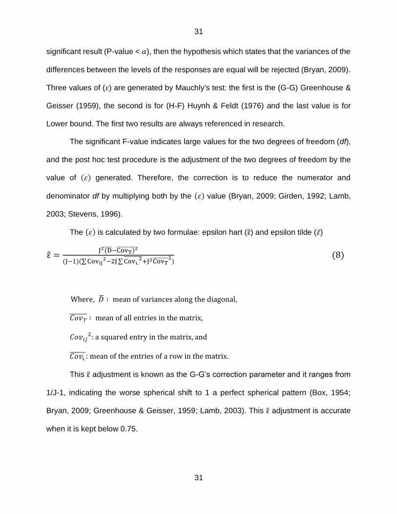
The (120576) is calculated by two formulae epsilon hart (ε) and epsilon tilde (120576)
ε =J2(D minusCovT) 2
(Jminus1)(sum Covij2minus2J sum Covi
2 +J2CovT 2) (8)
Where ∶ mean of variances along the diagonal
119862119900119907119879 ∶ mean of all entries in the matrix
1198621199001199071198941198952 a squared entry in the matrix and
119862119900119907119894 mean of the entries of a row in the matrix
This ε adjustment is known as the G-Grsquos correction parameter and it ranges from
1J-1 indicating the worse spherical shift to 1 a perfect spherical pattern (Box 1954
Bryan 2009 Greenhouse amp Geisser 1959 Lamb 2003) This ε adjustment is accurate
when it is kept below 075
32
32
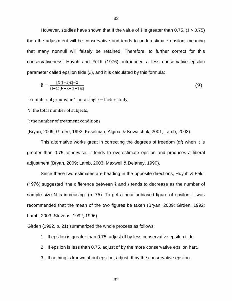
However studies have shown that If the value of ε is greater than 075 (ε gt 075)
then the adjustment will be conservative and tends to underestimate epsilon meaning
that many nonnull will falsely be retained Therefore to further correct for this
conservativeness Huynh and Feldt (1976) introduced a less conservative epsilon
parameter called epsilon tilde (120576) and it is calculated by this formula
ε =[N(Jminus1)ε]minus2
(Jminus1)[Nminuskminus(Jminus1)ε] (9)
k number of groups or 1 for a single minus factor study
N the total number of subjects
J the number of treatment conditions
(Bryan 2009 Girden 1992 Keselman Algina amp Kowalchuk 2001 Lamb 2003)
This alternative works great in correcting the degrees of freedom (df) when it is
greater than 075 otherwise it tends to overestimate epsilon and produces a liberal
adjustment (Bryan 2009 Lamb 2003 Maxwell amp Delaney 1990)
Since these two estimates are heading in the opposite directions Huynh amp Feldt
(1976) suggested ldquothe difference between ε and ε tends to decrease as the number of
sample size N is increasingrdquo (p 75) To get a near unbiased figure of epsilon it was
recommended that the mean of the two figures be taken (Bryan 2009 Girden 1992
Lamb 2003 Stevens 1992 1996)
Girden (1992 p 21) summarized the whole process as follows
1 If epsilon is greater than 075 adjust df by less conservative epsilon tilde
2 If epsilon is less than 075 adjust df by the more conservative epsilon hart
3 If nothing is known about epsilon adjust df by the conservative epsilon
33
33
Robustness
From the previous studies it has been confirmed that normality is a very rare
almost unattainable and difficult assumption in the real-world dataset Micceri (1989)
analyzed 440 distributions from ability and Psychometric measures and discovered that
most of those distributions have extreme shifts from the normal distribution shape
including different tail weight and different classes of asymmetry (Blanca Arnau Lόpez-
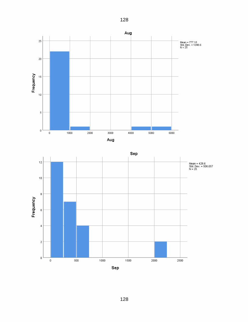
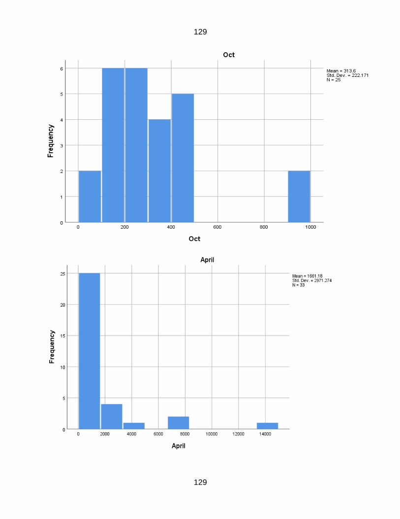
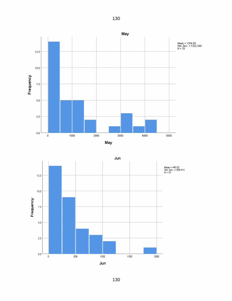
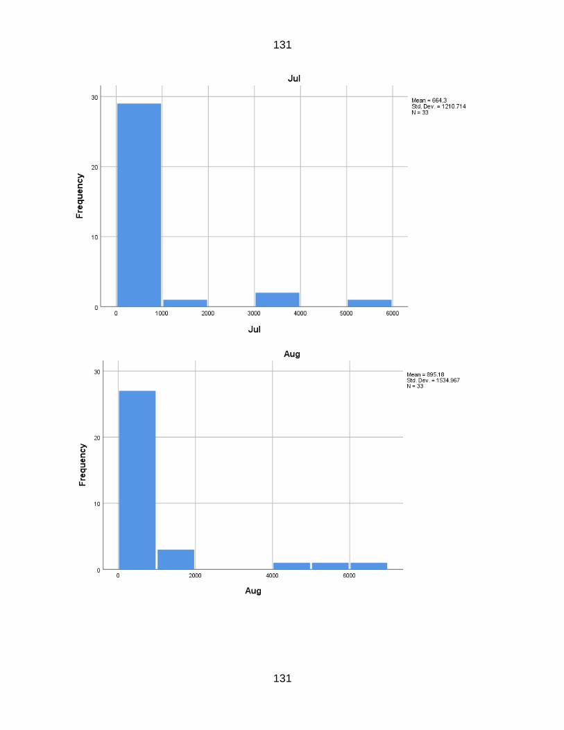
Montiel Bono amp Bendayan (2013) analyzed ldquo693 distributions derived from natural
groups formed in institutions and corresponding to 130 different populations with sample
sizes ranging from 10 to 30 399 of distributions were slightly non-normal 345 were
moderately non-normal and 26 distributions showed high contamination The
displayed skewness and kurtosis values were ranging between 026 and 175 He
therefore assert ldquothese results indicate that normality is not the rule with small samplesrdquo
(p 510) Other studies such as the works of (Harvey amp Siddique 2000 Kobayashi 2005
Van Der Linder 2006) have also established this fact Therefore researchers are faced
with the task of deciding whether the F-test is the best fit to analyze the real-world data
Robustness is the insensitivity of test statistics to the violation of the underlying
assumptions Ie robustness is when a statistical test still retains its properties of
rejecting a false null hypothesis and also the beta properties in the situation of
assumption violation However there should be a degree or an extent of violation of
assumptions a test statistic can reach before its type I error rate is inflated
Over the years there have been several ambiguous and very broad interpretations
given to the term ldquorobustnessrdquo of a test statistic which made it difficult for researchers to
determine the extent to which the F-test can be used when the distributions are non-
34
34
normal For example phrases like slightmoderate shift from normal distribution cannot
influence the results of the fixed-effects ANOVA (Montgomery 1991) Keppel (1982) puts
the same phrase as the violations of normality should not be a thing of worry unless the
violations are really to the extreme or F test is robust to moderate shift in location provided
the sample sizes are fairly large and equal across the treatment groups (Winer Brown amp
Michels 1991) Some opined that F-test is insensitive to a little shift in the location of
distribution shape (Berenson amp Levine 1992 Bridge amp Sawilowsky 1999 Harwell 1998
Kelley 1994 Sawilowsky amp Blair 1992) All the interpretations given to the term
robustness were relative to the basis of the research study This ambiguity problem also
made the study comparisons across different fields to be impossible (Blanca Alarcoacuten
Arnau Bono amp Bendayan 2017) Bradley (1978) summed the situation up in this
statement ldquoNot only is there no generally accepted and therefore standard quantitative
definition of what constitutes robustness but worse claims of robustness are rarely
accompanied by any quantitative indication of what the claimer means by the term In
order to provide a quantitative definition of robustness (of significance level) you would
have to state for a given alpha value the range of p-values for which the test would be
regarded as robustrdquo (p 145-146)
Therefore Bradley (1978) proposed a criterion that remedied the problem and
defined robustness as follows a test is robust if the type I error rate is 025 and 075 for
a nominal alpha level of 005 (Blanca Alarcoacuten Arnau Bono amp Bendayan 2017 p 533)
Bradley finally proposed liberal and stringent meanings of robustness The liberal
criterion which he defined as 05 alpha le π le 15 alpha alpha being the nominal
significance level π being the actual type I error rate Therefore a nominal alpha level of
35
35
05 would generate a p-value ranging from 0025 to 0075 and for the nominal alpha of
001 there would be a p-value range from 0005 to 0015 The stringent definition of
robustness is as follows ldquo09 alpha le π le 11 alpha thus a nominal alpha level of 005
would yield a p-value ranging from 0045 to 0055rdquo (Bridge 1996 Kelly 1994)
Power Analysis
It is important to carry out a priori statistical power analysis for the repeated
measures design However ldquocomplicated procedures lack of methods for estimating
power for designs with two or more RM factors and lack of accessibility to computer
power programs are among some of the problems which have discouraged researchers
from performing power analysis on these designsrdquo (Potvin 1996 p ii) Statistical power
is defined as the probability of finding a significant effect or a magnitude of any size of
differences when there exists a true effect among the population means (Park amp Schutz
1999)
Power analysis performed at the outset of an experimental study carries with it the
following benefits
I Power analysis helps researchers to determine the necessary number of subjects
needed to detect an effect of a given size Stevens (1999) noted ldquothe poor power
may result from small sample size (eg lt20 samples per group) andor from small
effect sizerdquo (p 126)
II Power analysis is performed before an experiment to determine the magnitude of
power a study carries given the effect size and the number of samples (Kupzyk
2011 Potvin 1996 Steidl Hayes amp Schauber 1997)
36
36
III It helps the researcher to answer such a question as does the study worth the
money time and the risk involved given the number of participants needed and
the effect sizes assumed (Potvin 1996)
IV Low power studies may ldquocut off further research in areas where effects do exist
but perhaps are more subtle eg social or clinical psychologyrdquo (Stevens 1999 p
126)
V ldquoIt also helps researchers to be familiar with every aspect of the studyrdquo (UCLA
2020)
The concept of power had existed for about four decades (Halow 1997) before
Cohen brought the concept to the limelight through his publications (Cohen 1962 1969)
The power of a statistical test was not thought of as a concept that can bridge the gap
between statistical significance and physical significance of a test (Thomas amp Juanes
1996) As soon as it is well known the significant contribution of power analysis to the
research process efforts have been made towards making its calculations very easy and
accessible Also practical methods for calculating statistical power and all its
components have been generated For some simple statistical designs several computer
software programs and power calculation tables have been made available to the
researchers (Borenstein amp Cohen 1988 Bradley 1978 1988 Cohen 1988 Elashoff
1999 Erdfelder Faul amp Buchner 1996 2007 Goldstein 1989) However for complex
designs analytical methods of estimating power are not easy to come by because more
factors result in higher interactions among the factors The methods of analyzing power
for the repeated measures ANOVA incorporates all factors that constitute the power
concept such as the correlations among the samples sample size the number of
37
37
treatment levels the population mean differences error variances the significance (α)
level and the effect sizes (Bradley 1978 Cohen 1988 Lipsey 1990 Potvin amp Schutz
2000 Winer Brown amp Michels 1991) Hence ldquothis method of estimating power function
is mathematically very complexrdquo (Park amp Schutz 1999 p 250) In RM ANOVA the
response variables are interdependent of each other the higher the correlations among
the variables the higher the power (Bryan 2009 Girden 1992 Keselman Algina amp
Kowalckuk 2001 Lamb 2003) ldquoThe outcome of the effect of all the factors that correlate
and affect power function in ANOVA designs can be described by what is called the non-
centrality parameter (NCP) The non-centrality parameter (NCP) is the magnitude of the
size of the differences between population means that represents the degree of inequality
between an F-distribution and the central (null hypothesis) F-distribution when the
observed differences in population means are not due to chance or sampling bias (Winer
et al 1991) There are quite a few methods of calculating a non-centrality parameter
(eg ƒ δ2 Φ λ) but all are closely related to each other and they all signify standardized
effect sizes This makes generalizability possible and comparable across studies (meta-
analysis) (Cohen 1988 Kirk 1995 Park amp Schutz 1999 Barcikowski amp Robey 1984
Tang 1938 Winer Brown amp Michels 1991) The non-centrality parameter λ for the one-
way RG ANOVA can be represented as
120582 =119899 sum( micro119894 minus micro)2
1205902 (10)
Where n is the sample size per group micro119894 represents the marginal (group) means micro is
the grand mean and 1205902 is the error variance (Bradley1978 Winer Brown amp Michels
1991) ldquoThe power is a nonlinear function of lambda (λ) the numerator and denominator
38
38
degrees of freedom of the F-test and the alpha level For an RM design the error
variance decreases as the degree of correlations among the levels of the RM factor
increasesrdquo This Lambda the unit of non-centrality for Repeated Measures design can be
derived by the following equations For the one-way RM ANOVA (j= 1 2hellipq)
120582 =119899 sum(micro119895minus micro)2
1205902 (1minus) (11)
(Park amp Schutz 1999 p251)
The non-centrality parameter measures the degree to which a null hypothesis is false
(Carlberg 2014 Kirk 2012) Invariably it relates to the statistical power of a test For
instance if any test statistic has a distribution with a non-centrality parameter that is zero
the test statistic (T-test Chi-square F-test) will all be central (Glen 2020) NCP is
represented by lambda (120582) and all the factors that affect power also affect lambda When
the null hypothesis is not true the one-way RM ANOVA has shifted from being centrally
distributed (Howell 1992 1999 Potvin 1996 Winer Brown amp Michels 1991) Therefore
power correlates with lambda in a quadratic manner that is nonlinear association
Path to Effect Sizes
When researchers are thrilled by the curiosity of knowing whether a difference exists
among groups because of an intervention or treatment given or not given they embark
on null hypothesis significance testing (NHST) Thompson (2003) puts it this way ldquoNHST
evaluates the probability or likelihood of the sample results given the sample size and
assuming that the sample came from a population in which the null hypothesis is exactly
truerdquo (p 7) However studies have shown that this statistical analysis is not an end in itself
but a means to an end (generalization to the population) The sixth edition of the APA
(2010) condemned the sole reliance on NHST by ldquonot only encouraging psychology to
39
39
shift emphasis away from NHST but also more fundamentally to think quantitatively and
cumulativelyrdquo (Fidler Thomason Cumming Finch amp Leeman 2004 Fidler 2010 p 2)
Therefore ldquoAPA stresses that NHST is but a starting point and that additional reporting
elements such as effect sizes confidence intervals and extensive description are
neededrdquo (APA 2010a p 33)
P-value only gives the probability that an effect exists given that the hypothesis of
no effect is true that is p (data | hypothesis) (Nakagawa amp Cuthill 2007 Sullivan amp Feinn
2012) Simply put the p-value is the probability that any disparity displayed among the
groups is only attributable to chance or sampling variations (bias) Statistical significance
is the interpretation of a test result given by the p-value in comparison to the level of
significance (plt alpha) (Kim 2015)
Statistical significance and p-value are a function of both effect size and sample
size therefore given a large enough number of samples even a very infinitesimal
difference can display a misleading result and lead to waste of resources (Aarts Akker
amp Winkens 2014 Kim 2015 Maher Markey amp Ebert-May 2013 p 346 Sullivan and
Feinn 2012) and on the other hand with fewer sample size the analysis carries no
power to detect significance Alpha level (level of significance) is the probability of
rejecting the null hypothesis when it is true It is the measure of how compatible the
sample data are with the null hypothesis Also the results given by the p-values make
the researchers resolve to a two-way (dichotomous) decision Either there is an effect
reject the Ho or effect does not exist fail to reject the null hypothesis Significant testing
alone cannot give information about the size of the difference that exists among groups
and also does not give a range of values (precision) around the effect of treatment or
40
40
intervention within which the value of the effect should be contained This is the
Confidence Interval Dependence on statistical significance poses difficulty to the meta-
analysis (studies will not be comparable across studies) (Maher Markey amp Ebert-May
2013)
All these demerits are found with the use of the NHST and to overcome these pitfalls
researchers crave a better alternative- Effect size
Meaning and importance of Effect size in Research
The Task Force on Statistical Inference of the American Psychological Association
understands the importance of Effect Size (ES) and has suggested that researchers
ldquoshould always provide some Effect Size estimates when reporting a p-valuerdquo
(WILKINSON amp TASKFORCE 1999 p 599) it stressed on reporting the effect sizes
alongside their interpretation ldquoWherever possible base discussion and interpretation of
results on point and interval estimatesrdquo (APA 2010 p 34) and finally gives detailed
standards for reporting meta-analyses ldquoreporting and interpreting Effect Sizes in the
context of previously reported effects is essential to good researchrdquo (p599) Effect size
gives information as to whether the observed difference is large enough to make sense
in real life or the context of the field of the research (clinical biological physical or
educational fields) ES can also signify the direction of the variability between groups or
the association between 2 groups of samples Different fields of knowledge have used
the term Effect size to report differences among group means eg education (Baird amp
Pane 2019 Kraft 2018 Lipsey 2012 Sawilowsky 2006) medicine and sciences
(Aarts Akker amp Winkens 2014 Akbaryan 2013 Kim 2015 Maher Markey amp Ebert-
May 2013 Nakagawa amp Cuthill 2007) psychology (Bakeman 2005 Durlak 2009
41
41
Schaumlfer amp Schwarz 2019) Effect sizes have been defined from various perspectives but
they all boil down to the same meaning Nakagawa amp Cuthill (2007) gave three definitions
of ES
ldquoFirstly the effect size can mean a statistic which estimates the magnitude of an
effect (eg mean difference regression coefficient Cohenrsquos d correlation
coefficient) It is called lsquoeffect statisticrsquo or lsquoeffect size indexrsquo Secondly it also means
the actual values calculated from certain effect statistics (eg mean difference =
30 or r =07 in most cases ES is written as lsquoeffect size valuersquo) The third meaning
is a relevant interpretation of an estimated magnitude of an effect from the effect
statistics This is sometimes referred to as the biological importance of the effect
or the practical and clinical importance in social and medical sciencesrdquo (p 593)
Deep insight into the meaning of effect size has provided an answer to the following
questions
bull Is there a real effect noticed beyond that which can be attributed to chances
bull If there is truly an effect what is the size of such treatment effect
bull How physically important is the size of such an effect (Bakker et al 2019 Kirk
2001)
ldquoEffect size is a way to measure or quantify the effectiveness of an intervention
treatment or program ES can also be described as the degree of falsity of the null
hypothesisrdquo ( (Descocircteaux 2007 p 25) An estimate of ES in conjunction with power
analysis is used to determine the sample size needed for the analysis This must be
carried out before the experimental procedures and is called prospective or a priori power
analysis
Reporting the effect sizes for significant p-value is believed to be the norm however
studies have shown that ldquoeven the p-values that are not significant should have their effect
sizes reportedrdquo (Thompson 1996 p 29)
42
42
Methods of calculating Effect Sizes
There are various methods of obtaining or calculating the effect sizes The first and simple
one that comes to mind is the direct group means comparison This is the effect size that
is calculated by comparing the raw group means ie micro1 minus micro2 However this
estimate is not generalizable to other studies since the variable of each study is scaled
according to the intentions of the researcher Even studies conducted in the same field
of study might not have the same dependent variables hence the scales are different
(Durlak 2009 Ladesma Macbeth amp Cortada de Kohan 2009) Research studies are
meant to complement each other therefore new knowledge should be developed upon
the existing ones Consequently researchers clamor for a better effect size estimator ndash
standardized effect size or standardized group mean difference
There are about three possible methods under this group When comparisons involve
only two groups of mean values Cohenrsquos d is the most used effect size estimator This is
a further step from the raw score mean difference estimator by standardizing the
difference through the pooling of the two groups Standard Deviations (SD) Cohenrsquos d is
only useful when the groupsrsquo SDs are very close and the distributions of the samples are
approximately normal (Cohen 1988 1992 Maher Markey amp Ebert-May 2013)
119889 = 119872119864minus119872119862
119878119886119898119901119897119890 119878119863 119901119900119900119897119890119889 119883 (
119873minus3
119873minus225) 119883 radic
119873minus2
119873 (12)
And
SD pooled =radic(119878119863119864)2+ (119878119863119862)2
2 (13)
43
43
However when the sample sizes significantly vary Hedge proposed pooling the SDs
from data that violate the homogeneity of variance assumption
119892 = 119872119864minus119872119862
119878119863 119901119900119900119897119890119889 (14)
119878119901119900119900119897119890119889=radic((119899119864minus1)119878119863119864 +
2 (119899119862minus1)1198781198631198622)
(119899119864 + 119899119862)minus2 (15)
The third method assumes that the control group SD is closer to the population SD so it
uses the control group SD to standardize the mean difference ( (Glass McGraw amp Smith
1981) Glassrsquos delta is represented by
Δ = micro 1minusmicro 2
119878119863119888119900119899119905119903119900119897 (16)
There are various approaches to converting these metrics among each other eg
Cohenrsquos d to Hedgesrsquo g point biserial to Cohenrsquos d etc (For further readings see Durlak
2009 Ladesma Macbeth amp Cortada de Kohan 2009 Maher Markey amp Ebert-May
2013) Another method that is equally useful in educational research is the correlation
coefficient This measures the relationships between two groups of variables The
magnitude of the association can range from a negative one (-1 indicating perfect inverse
proportion) to zero (0 indicating no linear relationship) and a positive one (+1 indicating
perfect direct proportion) For this the Pearson correlation coefficient (r) is used and the
formula is 119903 =119878119909119910
119878119863119909119878119863119910 where r is the Pearson r 119878119909119910 is the covariance of the groups and
119878119863119909119878119863119910 is the product of the grouprsquos SDs
44
44
Effect Size for More Than Two Group Means
Cohenrsquos f
When the number of groups has increased to more than two Cohen (1988) suggested
the use of the parameter he proposed to be Cohenrsquos f for estimating the effect size The
flaw in this method is that there is no distinguishing factor among the group means it is
just to reach a dichotomous decision of either the group means are equal or not The
method is to normalize the sum of the deviations of the sample means from the combined
sample mean to the combined sample SD The formula is
119891 =120590119898
120590 120590119898 = radic
Σ(119898119894minus2
119896 (17)
119896 119905ℎ119890 119899119906119898119887119890119903 119900119891 119904119886119898119901119897119890 119892119903119900119906119901119904
119898119894 ∶ 119898119890119886119899 119900119891 119892119903119900119906119901 119894 119886119899119889
119898119890119886119899 119900119891 119896 119904119886119898119901119897119890 119898119890119886119899119904 119886119899119889
120590 119901119900119900119897119890119889 119878119889 119900119891 119896 119904119886119898119901119897119890 119892119903119900119906119901119904
There are other measures of effect size that are appropriate for
ANOVA ANCOVA and MANCOVA which are the Eta-Squared and Partial
Eta-Squared Eta-Squared is the ratio of the between-group sum of
squares to the total sum of squares while the partial Eta-squared is the
ratio of the between-group sum of squares to the sum of the between-
groups sum of squares and the error sum of squares (Maher Markey amp
Ebert-May 2013 For further details on these effect sizes and the new
methods see Bakeman 2005 Cohen 1973 Kerlinger 1964)
45
45
Eta-Squared is calculated thus
1205782 = 119878119878119887119890119905119908119890119890119899
119878119878119905119900119905119886119897 119878119878 119904119906119898 119900119891 119904119902119906119886119903119890119904 (18)
While the partial Eta-Squared is calculated thus
1205781199012
119878119878119887119890119905119908119890119890119899
119878119878119887119890119905119908119890119890119899 + 119878119878119890119903119903119900119903 119878119878 119904119906119898 119900119891 119904119902119906119886119903119890119904 (19)
46
46
CHAPTER THREE
METHODOLOGY
The goals of this study are (1) to confirm and establish that the real-world data usually
deviate from normality assumptions no matter the field of study (2) to compare the Type
I error rates and the comparative power of the statistical methods of comparing the
differences in population means when correlated groups or dependent samples are
involved The two hypothesis tests involved are (1) The parametric one-way repeated
measures (2) The nonparametric Friedmanrsquos test
Background of the Data
Early in 2020 the Centers for Diseases Control and Prevention (CDC) announced the
breakout of a virus in the family of severe acute respiratory syndrome coronavirus 2
(SARS-CoV-2) The world health organization (WHO) termed the novel virus the
coronavirus disease 2019 or COVID-19 (CDC 2020) According to CDC the COVID-19
is highly contagious spreading from human to human Although research is still ongoing
to unravel all the details about the disease significant information about its nature such
as the mode of spread maturation and symptoms have been reported The disease can
be contracted through close contact with the droplets (sneezing coughing) from the
infected individuals The first case of the virus in the United States was confirmed in
Washington State in February 2020 Within a month cases had been reported in about
six states By March 2020 the virus had spread exponentially across all the states in the
US Studies showed that the spread of the virus was more rapid in areas with large
gatherings of people in close proximities Examples of such gatherings include religious
places restaurants and cafes schools gyms and other indoor recreation centers
47
47
Consequently governments imposed some control measures such as stay-at-home
orders lockdowns and restricted movements to reduce the spread from person to
person Each state implemented the measures differently and at various times The data
about the COVID-19 including daily spread daily death counts by age daily death count
by gender and daily death counts by race hospitalizations and other underlying
conditions relating to COVID-19 are available on the John Hopkins University website
and the Centers for Disease and Control prevention website
The weekly death count data was obtained from the CDC website and were
grouped into April and May (9 weeks) June and July (8 weeks) and Aug and Sept (9
weeks) The first nine weeks represent the times of implementation of the lockdown
measures by different states during the eight weeks group the measures such as
wearing of masks and social distancing were still in place but the movement of people
had increased during the last nine weeks group the people moved freely restaurants
dine-ins were opened for few people to gather also libraries allow readers to come in and
study people gathered at events and finally schools were opened for students stores
were operating normally etc
The Method of Sampling
Since the pandemic hit different states at varying degrees the daily mortality was
different among the states Some states did not experience the breakout at the beginning
of the outbreak some had fluctuations in their case rates while other states reported
increasing cases daily eg New York Therefore out of the 50 states 37 states were
first sampled based on the completeness of the weekly death counts data with very few
states having one or two missing counts These figures were grouped in the following
48
48
order April and May total death count data (9 weeks) June and July total death count
data (8 weeks) Aug and Sept total death counts data (9 weeks) Afterward four states
out of the 37 previously sampled states were dropped because of incomplete case
records The total number of samples was 33 states having complete records of mortality
count for 7 months (April-Oct) A resampling was done after the first sampled data had
been plotted in histograms The shapes of the distributions generated with these grouped
data correspond with previous studies on the issue of normality This confirmed the
assumption of normality as a rare concept in real-life data From these chosen statesrsquo
data random sampling of different sizes was performed with replacement
(n=5812182533) using Excel 2016
Methods of Analysis
The analysis was conducted on differing sizes of samples randomly selected from
the 33 states dataset The samples are in the following orders (N=5812182533) The
nominal alpha was set at 005 the test statistic used for the repeated measures ANOVA
was the F and the test statistic for Friedman was Fr There was no treatment administered
to any of the groups however the data represents a longitudinal observation of the
weekly mortality counts that occurred in each month for different states The null
hypothesis of interest is that of no differences among the group means The null
hypothesis assumes that the distributions of the observations within each block come
from the same parent distribution The alternative hypothesis is that at least one of the
group means is different This design is a randomized complete block with one
observation per treatment-block combination
49
49
For the first part of the objective of this study the selected datasets were grouped
in varying orders For example six months data out of the seven months were grouped
by two months (April to May total death counts June to July total death counts Aug to
Sept total death counts) Descriptive analyses were performed on the 37 total samples
to observe the basis of normality assumption and the extent of their violations Therefore
the distribution results were compared against the normal curve
Three Major Distributions and their Characteristics
The normal distribution is represented by a bell shape or curve with a line dividing
the curve into equal halves known as symmetry The first half of the curve mirrors the
other half Gaussian distribution was named after the author Carl Friedrich Gauss in
1809 who discovered the normal distribution to rationalize the method of least squares
(wikipediaorg) This distribution has a mean (micro) of 0 and standard deviation (σ) of 1 This
implies that the mean and the median are equal Skewness and kurtosis are the third and
fourth moments of the normal distribution The skewness for the normal distribution is set
at zero (0) and the kurtosis is set at three (3)
The probability density function is
Pu(120583) = (radic2120587)minus1 exp(minus12u2) (20)
Skewness and kurtosis are common descriptive properties that quantify violations from
normality (Glass et al 1978)
Skewness signifies how long the tail of the distribution is It measures how
symmetry or not symmetry the shape of the distribution looks In normal distribution
skewness = 0 Symmetry can be either tilted to the left of the distribution with a long tail
to the right this is often termed the positive skewness This happens when the mean of
50
50
the distribution is greater than the median and the mode and the bulk of the scores are
close to zero Whereas when the bulk of the scores are tilting towards the right of the
distribution and long tail towards the left this is called negative skewness The median is
greater than the mean in this distribution
For univariate data Y1 Y2 hellip YN the formula for skewness is
1198921 = sum (119884119894minus)3119873
119894=1 119873
1198783 (21)
Where is the mean S is the standard deviation and N is the number of sample
size Note that in computing the skewness the S is computed with N in the denominator
rather than N minus 1 ldquoThis formula for skewness is referred to as the Fisher- Pearson
coefficient of skewnessrdquo
Kurtosis represents the shape of the peak of the distribution ie how tall or short
the peak looks like For a normal distribution kurtosis = 300 Any distribution that displays
a kurtosis value larger than 3 signifies a very long peak This is called leptokurtic and as
the kurtosis value falls below 3 the peak becomes smallerflatter this is playkurtic
Kurtosis = sum (119884119894minus119886119884 )
4119873119894=1 119873
1198784 minus 3 (22)
Three is subtracted from the value generated by the formula so that the standard
normal distribution has a kurtosis of zerordquo (Methods 2020 p 13511)
51
51
Figure 2Gaussian (Normal) Distribution
Chi-Square Distribution when chi-square carries only two degrees of freedom it is
usually referred to as exponential The chi-square is calculated by subtracting the
expected outcome from the observed outcomes The probability function is
119901119909(119883) = 120590minus1 exp [minus(119909minus120563)
120590] (119909 gt 120563 120590 gt 0 (23)
52
52
Figure 3Chi-Square Distribution
The uniform distribution The peak of this type of distribution of data is usually flat at the
top The histogram is rectangular in shape and all the outputs are equally likely The
probability function of a uniform distribution is as follows
119875119884(119910) = (120573 minus 120572)minus1 (120572 le 119910 le 120573 (24)
53
53
Figure 4Uniform Distribution
All three distributions were adapted from Sawilowsky amp Fahoome (2003)
The Descriptive Analysis
The April amp May dataset has a mean of 267619 median = 96900 standard
deviation = 3934957 IQR = 2210 skewness = 2654 and kurtosis = 7799 This dataset
has an 1153 variance (leptokurtic) from normal kurtosis June amp July dataset displays
a mean of 104103 median of 68200 standard deviation of 1438659 IQR = 755
skewness of 2993 (positively skewed) and kurtosis = 8841 demonstrating a
1947above the normal kurtosis The August amp Sept dataset showed a mean of
134138 median of 748 standard deviation of 1966657 IQR of 1050 positive skewness
of 2834 and kurtosis of 7445 This is 1482 more kurtotic than the normal distribution
kurtosis The results of the histograms are displayed in Appendix A
54
54
The outputs of the histograms in figures 2-4 were consistent with the previous
findings of Micceri (1989) and Blanca Arnau Lόpez-Montiel Bono amp Bendayan (2013)
on how real-life datasets have violated the assumption of normality
Also the samples were randomly re-selected with replacements analyzed with the
number of repeated measures equals 7 in each number of samples the results of the
analysis showed a little variation from the ones displayed earlier However it was also
not inconsistent with prior findings The distributions of output display mostly the Chi-
Square distribution The histograms are displayed in Appendix B
To check for the multivariate normality assumption some random numbers were
computed with the standardized residuals of the variables in SPSS 2601 These
values were used to plot the histograms with the normal curves The results are as
follows Uniform distributions and multimodal distributions seemed to be common in the
results There was a trace of normality as the sample sizes increased from 12 through
33 confirming the central limit theorem In conclusion the assumption of normality is
hardly met in the real-world distributions
55
55
Figure 5 Multivariate Normal Distribution for Sample Size of 5 k=7
Figure 6 Multivariate Normal Distribution for Sample Size of 8 k=7
56
56
Figure 7 Multivariate Normal Distribution for Sample Size of 12 k=7
Figure 8 Multivariate Normal Distribution for Sample Size of 18 k=7
57
57
Figure 9 Multivariate Normal Distribution for Sample Size of 25 k=7
Figure 10 Multivariate Normal Distribution for Sample Size of 33 k=7
Steps Followed in the Methods of Analysis
58
58
Differing combinations of n and k were considered (n=5812182533 and k= 35 amp7)
To compute 119865119903 statistic data were ordered from least to greatest within each block
independently 119903119894119896 is the rank of 119883119894119896 in the 119894119905ℎ block and average rank were assigned via
the within-blocks ranking method The test is significant if the calculated result is greater
than the tabulated values the decision is to reject the null hypothesis The current
mortality data were analyzed using the Repeated measures ANOVA test according to
equation 17
119865 =119872119904119861
119872119904119864 (25)
MSB is the Mean Square Between or Mean Square for the Treatments or Conditions
and the Mean Square Error is the within mean square that will remain after the MSs Mean
Square Subjects or Participants has been removed Thereby enhances higher power
Friedmanrsquos test will be analyzed according to either of these two formulae The two
formulae both arrive at the same answer
Xr2 =
12
bk(k+1)sumℝj
b(k+1)2
2 (26a)
1198831199032 =
12
119887119896(119896 + 1)120564119877119869
2 minus 3119887(119896 + 1) (26b)
The effect size was calculated using the GPower 3194 ldquoIn GPower there is an effect
size calculator or effect size drawer ldquoEffect size drawer has the possibility of computing
the effect size f from the variance explained by the tested effect and error variancerdquo
(Faul et al 2007) Eta squared (η2) or effect size f as defined by Cohen (1988) is used in
59
59
almost all ANOVA procedures Cohen stated the values for the effect size f as 01 for the
small effect 025 for the medium effect and 04 for the large effect size Since this is raw
data tabular visualization of the observation (histogram normal curve box plot etc) was
generated and the q-q plot was used to determine the normality of the observations
Mauchlys W test was calculated to determine to what extent the sphericity assumption
was met and if there are cases of sphericity assumption violation necessary corrections
of the degrees of freedom were performed Shapiro-Wilks test of normality was reported
since the Kolmogorov-Smirnov test is always not strong enough to correctly reject the
false null The non-centrality parameter is the expected joined effect of all the factors on
power in ANOVA design Non-centrality parameter is required to calculate the power for
the Friedmanrsquos test in GPower 3194 software
All computations were carried out using SPSS 26 and GPower 3194 The results of all
the analyses are reported in the next chapter
60
60
CHAPTER FOUR RESULTS
RESULTS AND DISCUSSION
The 37 states mortality counts were represented on a histogram to compare the
shapes of the outcome variables with the prevailing three distribution shapes normal bell
curve Uniform and Chi-Square distributions Statistical analyses were performed to
investigate the Type I error rates and the comparative power properties of the two tests
the repeated measures and Friedmanrsquos test for differing sample sizes and different
condition group combinations Six sample sizes (n = 5812182533) and number of
conditions (k = 357) were used to perform the analysis SPSS 2601 was used to
compute the effect sizes for the repeated measures in the form of partial eta squared
and the effect size for the Friedmanrsquos test in the form of Kendallrsquos W The results of all
the Type I error rates for the two tests under differing sample sizes and group
combinations are presented in the tables below
Type I Error Rates
Table 2 Type I Error Rates when α=005 with G-G correction
Sample size ampnumber of k Rep M119890119886119904
G minus G correction Friedmanrsquos Test
119899119896 = 5 119896 = 3 0245 Nil 0091
119899119896 = 5 119896 = 5 0547 0740 0308
119899119896 = 5 119896 = 7 0450 0557 0515
119899119896 = 8 119896 = 3 0015 Nil 0008
119899119896 = 8 119896 = 5 0236 0184 0004
119899119896 = 8 119896 = 7 0155 0044 0001
61
61
119899119896 = 12 119896 = 3 0007 Nil 0028
119899119896 = 12 119896 = 5 0183 0111 0015
119899119896 = 12 119896 = 7 0176 0072 0010
119899119896 = 18 119896 = 3 0080 0046 0000
119899119896 = 18 119896 = 5 0061 0007 0000
119899119896 = 18 119896 = 7 0053 0001 0001
119899119896 = 25 119896 = 3 0080 0047 0000
119899119896 = 25 119896 = 5 0126 0055 0000
119899119896 = 25 119896 = 7 0082 0008 0000
119899119896 = 33 119896 = 3 0021 0006 0000
119899119896 = 33 119896 = 5 0065 0013 0000
119899119896 = 33 119896 = 7 0026 0000 0000
The following tables 3-5 below showed the original robustness of the repeated measures
with the follow up Greenhouse-Geisser corrections for the significant Mauchleyrsquos W test
Rates of Errors with the Greenhouse- Geisser Corrections
Table 3 Type I Error Rates for k=3and G-G corrections
119881119886119903119894119900119906119904 Samples when k = 3 Mauchlyprimes W Error Rates (119877119872) Type I Error(G minus G) Error Rates (119865119903)
1198991 = 1198992 = 1198993 = 5 119878119894119892119899119894119891119894119888119886119899119905 0245 Nill 0091
1198991 = 1198992 = 1198993 = 8 119878119894119892119899119894119891119894119888119886119899119905 0015 0021 0008
1198991 = 1198992 = 1198993 = 12 119878119894119892119899119894119891119894119888119886119899119905 0007 Nill 0028
1198991 = 1198992 = 1198993 = 18 119878119894119892119899119894119891119894119888119886119899119905 0046 0080 0000
1198991 = 1198992 = 1198993 = 25 119878119894119892119899119894119891119894119888119886119899119905 0049 0080 0000
1198991 = 1198992 = 1198993 = 33 119878119894119892119899119894119891119894119888119886119899119905 0006 0021 0000
62
62
Table 4 Type I Error Rates for k=5and G-G corrections
Table 5 Type I Error Rates for k=7and G-G corrections
Effect Sizes Partial Eta Squared and the Kendallrsquos W
Table 6 Partial Eta squared for RM amp Kendallrsquos W for Fr test
Sample size ampnumber of repeated measures (rm)
Partial Eta Squared (η2)
Kendallrsquos W
1198991 = 1198992 = 1198993 = 5 119896 = 3 0296 0480
119899119896 = 5 119896 = 5 0110 0240
119899119896 = 5 119896 = 7 0172 0174
119899119896 = 8 119896 = 3 0451 0609
119881119886119903119894119900119906119904 Samples when k = 5 Mauchleyrsquos W significance
Type I Error Rates (RM)
Type I Error Rates (G-G)
Type I Error Rates (Fr)
1198991 = 1198992 = 1198993 = 1198994 = 1198995 = 5 Not Significant 0740 0547 0308
1198991 = 1198992 = 1198993 = 1198994 = 1198995 = 8 Not Significant 0184 0236 0004
1198991 = 1198992 = 1198993 = 1198994 = 1198995 = 12 Not Significant 0111 0183 0015
1198991 = 1198992 = 1198993 = 1198994 = 1198995 = 18 Significant 0007 0061 0000
1198991 = 1198992 = 1198993 = 1198994 = 1198995 = 25 Significant 0055 0126 0000
1198991 = 1198992 = 1198993 = 1198994 = 1198995 = 33 Significant 0013 0065 0000
119881119886119903119894119900119906119904 Samples when k = 7 Mauchleyrsquos W significance
Type I Error Rates (RM)
Type I Error Rates (G-G)
Type I Error Rates (Fr)
1198991 = 1198992 = 1198993 = 1198994 = 1198995 = 1198996 = 1198997 = 5 Significant 0557 0450 0515
1198991 = 1198992 = 1198993 = 1198994 = 1198995 = 1198996 = 1198997 = 8 Significant 0044 0155 0001
1198991 = 1198992 = 1198993 = 1198994 = 1198995 = 1198996 = 1198997 = 12 Significant 0072 0176 0010
1198991 = 1198992 = 1198993 = 1198994 = 1198995 = 1198996 = 1198997 = 18 Significant 0001 0053 0001
1198991 = 1198992 = 1198993 = 1198994 = 1198995 = 1198996 = 1198997 = 25 Significant 0008 0082 0000
1198991 = 1198992 = 1198993 = 1198994 = 1198995 = 1198996 = 1198997 = 33 Significant 0000 0026 0000
63
63
119899119896 = 8 119896 = 5 0193 0484
119899119896 = 8 119896 = 7 0255 0478
119899119896 = 12 k = 3 0360 0299
119899119896 = 12 k = 5 0154 0257
119899119896 = 12 k = 7 0157 0233
119899119896 = 18 k = 3 0166 0531
119899119896 = 18 k = 5 0185 0280
119899119896 = 18 k = 7 0195 0207
119899119896 = 25 k = 3 0119 0386
119899119896 = 25 k = 5 0091 0225
119899119896 = 25 k = 7 0112 0188
119899119896 = 12 k = 3 0147 0387
119899119896 = 33 119896 = 5 0094 0190
119899119896 = 33 119896 = 7 0124 0169
The effect sizes generated from the SPSS 2601 showed that the Kendallrsquos W which is
the effect size for the Friedmanrsquos test displayed higher values than the effect size values
of the repeated measures ANOVA It was only in one situation (1198991 = 1198992 = 1198993 = 5 119896 =
7) that the effect size for the two tests nearly overlapped (η2 =0172 Kendallrsquos W =
0174) but Kendallrsquos W still supersedes When 1198991 = 1198992 = 1198993 = 12 119896 = 3 RM has slightly
higher effect than the Friedman (η2 = 0360 Kendallrsquos W = 0299) It showed the extent
to which Friedmanrsquos test has greater power to detect differences among a group of
means even when the parametric assumptions have been violated the rate at which
64
64
Friedmanrsquos test detects differences was as high as 609 whereas the RM did not pass
the level of 451 Table 6 above displays the results
Table 7 The Sphericity Assumption Results
Sample size ampnumber of repeated measures (rm)
Mauchlyrsquos W
1198991 = 1198992 = 1198993 = 5 119896 = 3 0138
119899119896 = 5 119896 = 5 0007
119899119896 = 5 119896 = 7 0000
119899119896 = 8 119896 = 3 0592
119899119896 = 8 119896 = 5 0000
119899119896 = 8 119896 = 7 0000
119899119896 = 12 119896 = 3 0753
119899119896 = 12 119896 = 5 0000
119899119896 = 12 119896 = 7 0000
119899119896 = 18 119896 = 3 0000
119899119896 = 18 119896 = 5 0000
119899119896 = 18 119896 = 7 0000
119899119896 = 25 119896 = 3 0000
119899119896 = 25 119896 = 5 0000
119899119896 = 25 119896 = 7 0000
119899119896 = 33 119896 = 3 0000
119899119896 = 33 119896 = 5 0000
119899119896 = 33 119896 = 7 0000
65
65
Table 7 displayed the results of the assumption of sphericity (equal variances and equal
standard deviations across groups) It was obvious that this assumption was met in only
three sample groups out of the total of eighteen sampled groups The groups were N= 5
8 and 12 with the combinations of three groups of repeated measures This assumption
was violated in the subsequent sample groups This is an evidence that it is only in smaller
samples that the assumption of either homogeneity or sphericity is established
Comparative Power Analysis
The summaries of the power analysis as a function of the three Effect sizes as stated by
Cohen (1988) f for small effect is 01 medium effect is 025 and large effect is 04 were
given in details below As previously stated there were six samples of equal sizes of n=
5812182533 each of which was combined with different numbers of repeated
measures (k= 357) With each combination power of the repeated measures ANOVA
and the nonparametric alternative Friedmanrsquos tests were computed The y-axis
represents the power (1-Beta) label and it ranges from 0 to 100 When a test displays a
power of zero (0) it signifies that such a test has no power to detect differences among
means Whereas a power level equivalent to one (1) means that the test has maximum
power to find even the slightest significance among group means The x-axis displayed
the effect sizes labels 010sd 025sd amp 040sd the ldquosdrdquo is the standard deviation of each
sample group The actual effect size is the standard deviation of the groups multiplied by
the constants (effect size benchmarks) before them The power curve was obtained
through the GPower 3194 To compute the power curve for Friedmanrsquos test a non-
centrality parameter corresponding to each sample size from the repeated measures
ANOVA was used The values from the two power curves were obtained and plotted on
66
66
both the line graph and bar graphs for different alpha levels (001 005 01) Although
the results for the three significant levels were displayed in a table in this study the power
curves for only α= 005 were presented in the result since 005 alpha level is prevalent
in research studies The bar graphs will be referenced in Appendices A-B
Differing Sample Sizes and Differing Condition Groups
Sample 119951120783 = 119951120784 = 119951120785 = 120787
The first group of number sampled was n1=n2=n3=5 with the number of treatments
to be three (n=5 k=3) The alpha level is set at 005 This sample group yielded powers
of 01 and 099 with shift of 01σ for the Repeated Measures ANOVA (RMA) and the
Friedmanrsquos test At shift 025σ the powers were 211 for RMA and 219 for Friedmanrsquos
test and at the 04σ there was 384 power for RMA and 396 for Friedmanrsquos test Except
for the 1σ that gave about the same power the Friedmanrsquos test gave more power than
the RMA
Figure 11 Comparative Power rate for the RM amp Fr for n=5k=3
67
67
Sample 119951120783 = 119951120784 = 119951120785 = 119951120786 = 119951120787 = 120787
The next sample group was kept unchanged and the treatment groups increased
to 5 At 1σ the power for RMA was 128 whereas it was 156 for the Freidmanrsquos test
For effect size of 25σ the powers were 322 for RMA and 421 for Friedmanrsquos test and
for 04σ the power was 605 for RMA and 747 for Friedmanrsquos test The Friedmanrsquos test
demonstrated power advantage all through over the RMA
Figure 12 Comparative Power rate for the RM amp Fr for n=5k=5
Sample n1=n2=n3=n4=n5=n6=n7=5
The next group that was explored was the same number of groups but the
repeated measures were increased again to 7 At 1σ the power for RMA was 152
whereas it was 219 for the Freidmanrsquos test For effect size of 25σ the powers were 420
for RMA and 605 for Friedmanrsquos test and for 04σ the power was 756 for RMA and
68
68
912 for Friedmanrsquos test Again the Friedmanrsquos test demonstrated higher power rates
over the RMA for all the effect sizes
Figure 13 Comparative Power rate for the RM amp Fr for n=5k=7
Sample 119951120783 = 119951120784 = 119951120785 = 120790
Another group of random samples that was explored was sample of eight and
treatments of three (Sample n1=n2=n3=8) In this group the effect size of 1σ gave the
power of 156 for RMA and 115 for the Freidmanrsquos test For effect size of 25σ the
powers were 394 for RMA and 294 for Friedmanrsquos test and for 04σ the power was 687
for RMA and 578 for Friedmanrsquos test Conversely the RMA demonstrated higher power
rates over the Friedmanrsquos test across all the effect sizes
69
69
Figure 14 Comparative Power rate for the RM amp Fr for n=8k=3
Sample 119951120783 = 119951120784 = 119951120785 = 119951120786 = 119951120787 = 120790
The next shift was calculated for sample groups of eight and treatment groups of
five For 1σ the power for RMA yielded 218 whereas it was 199 for the Freidmanrsquos
test And for effect size of 25σ the powers were 599 for RMA and 578 for Friedmanrsquos
test then for 04σ the power was 907 for both RMA and Friedmanrsquos test Except for the
04σ where both tests tallied for the remaining two shifts the RMA was a little bit higher
70
70
Figure 15 Comparative Power rate for the RM amp Fr for n=8k=5
Sample 119951120783 = 119951120784 = 119951120785 = 119951120786 = 119951120787 = 119951120788 = 119951120789 = 120790
The next group was the same number of groups but the repeated measures were
increased to 7 At 1σ the power for RMA yielded 273 whereas it was 294 for the
Freidmanrsquos test For effect size of 25σ the powers were 742 for RMA and 788 for
Friedmanrsquos test and for 04σ the power displayed 975 for RMA and 987 for Friedmanrsquos
test Again the Friedmanrsquos test gave higher power rates over the RMA for all the effect
sizes
71
71
Figure 16 Comparative Power rate for the RM amp Fr for n=8k=7
Sample 119951120783 = 119951120784 = 119951120785 = 120783120784
For this group of samples at the 1σ shift the power for RMA was 238 whereas
it was 135 for the Freidmanrsquos test For effect size of 25σ the powers were 613 for RMA
and 381 for Friedmanrsquos test and for 04σ the power was 902 for RMA and 730 for
Friedmanrsquos test Again the Friedmanrsquos test performed lower in terms of power than the
RMA for all the effect sizes with the differences ranging from 0103 to 0232
72
72
Figure 17 Comparative Power rate for the RM amp Fr for n=12k=3
Sample 119951120783 = 119951120784 = 119951120785 = 119951120786 = 119951120787 = 120783120784
For this group of samples at the 1σ shift the power for RMA was 351 whereas
it was 250 for the Freidmanrsquos test For effect size of 25σ the powers were 842 for RMA
and 730 for Friedmanrsquos test and for 04σ the power was 992 for RMA and 978 for
Friedmanrsquos test Again the Friedmanrsquos test performed lower in terms of power than the
RMA for all the effect sizes
73
73
Figure 18 Comparative Power rate for the RM amp Fr for n=12k=5
Sample 119951120783 = 119951120784 = 119951120785 = 119951120786 = 119951120787 = 119951120788 = 119951120789 = 120783120784
This sample group has the same number as the last two groups but the number
of repeated measures was increased to 7 At 1σ the power for RMA yielded 448 and
381 for the Freidmanrsquos test For effect size of 25σ the powers were 996 for RMA and
979 for Friedmanrsquos test and for 04σ the power displayed 1000 for RMA and 999 for
Friedmanrsquos test Here the RMA gave higher power rates over the Friedmanrsquos test for all
the effect sizes
74
74
Figure 19 Comparative Power rate for the RM amp Fr for n=12k=7
Sample 119951120783 = 119951120784 = 119951120785 = 120783120790
This group comprises of eighteen equal samples in three different groups
(n1=n2=n3=18) This sample group yielded powers of 365 161 with shift of 01σ for the
Repeated Measures ANOVA (RMA) and the Friedmanrsquos test At shift 025σ the powers
were 830 for RMA and 495 for Friedmanrsquos test and at the 04σ there was 988 power
for RMA and 866 for Friedmanrsquos test At 04σ level of shift the power discrepancy
between the RMA and Friedmanrsquos test was 0122 but over the RMA gave higher power
across all shifts
75
75
Figure 20 Comparative Power rate for the RM amp Fr for n=18k=3
Sample 119951120783 = 119951120784 = 119951120785 = 119951120786 = 119951120787 = 120783120790
This group of samples demonstrated the power of 543 at the 1σ shift for RMA
and 321 for the Freidmanrsquos test For effect size of 25σ the powers were 972 for RMA
and 866 for Friedmanrsquos test and for 04σ the power was 1000 for RMA and 998 for
Friedmanrsquos test The power difference was large at 1σ shift and decreased to about half
the difference 25σ shift The Friedmanrsquos test rose sharply to 0998 at the 04σ shift
trailing the RMA of 1000
76
76
Figure 21 Comparative Power rate for the RM amp Fr for n=18k=5
Sample 119951120783 = 119951120784 = 119951120785 = 119951120786 = 119951120787 = 119951120788 = 119951120789 = 120783120790
This is eighteen equal samples with seven number of measures It gave the power
of 677 at the 1σ shift for RMA and 495 for the Freidmanrsquos test For effect size of 25σ
the powers were almost the same for the two tests 996 for RMA and 979 for Friedmanrsquos
test And at 04σ the power was 1000 for both RMA and Friedmanrsquos test The power
discrepancy very was large at 1σ shift and decreased to almost negligible figure at 25σ
shift The RMA and Friedmanrsquos test rose to 1000 at the 04σ shift
77
77
Figure 22 Comparative Power rate for the RM amp Fr for n=18k=7
Sample 119951120783 = 119951120784 = 119951120785 = 120784120787
This group consists of twenty-five equal samples in three different groups
(n1=n2=n3=25) The powers were 504 and 189 at the 01σ shift for the Repeated
Measures ANOVA (RMA) and the Friedmanrsquos test At shift 025σ there was a very sharp
increase in the power curves which brought the powers for both tests to 944 for RMA
and 605 for Friedmanrsquos test At the 04σ shift Friedmanrsquos test increased drastically with
about 339 in power to almost the same power as RMA
78
78
Figure 23 Comparative Power rate for the RM amp Fr for n=25k=3
Sample 119951120783 = 119951120784 = 119951120785 = 119951120786 = 119951120787 = 120784120787
This group of random samples explored was twenty-five equal number in each
group and the number of measures was five (Sample n1=n2=n3=n4=n5=25) In this group
the effect size of 1σ shift demonstrated the power of 724 for RMA and 395 for the
Freidmanrsquos test For effect size of 25σ the powers were 997 for RMA and 944 for
Friedmanrsquos test and for 04σ the power was 1000 for both RMA and for Friedmanrsquos test
Conversely the RMA demonstrated higher power rates over the Friedmanrsquos test for the
first two effect sizes
79
79
Figure 24 Comparative Power rate for the RM amp Fr for n=25k=5
Sample 119951120783 = 119951120784 = 119951120785 = 119951120786 = 119951120787 = 119951120788 = 119951120789 = 120784120787
This is twenty-five equal samples with seven repeated measures It gave the power
of 852 for RMA and 605 for the Freidmanrsquos test at the 1σ shift For effect size of 25σ
the powers were almost the same for the two tests1000 for RMA and 996 and 979 for
Friedmanrsquos test And at 04σ the power was 1000 for both RMA and Friedmanrsquos test
The power discrepancy very was large at 1σ shift and decreased to almost negligible
figure at 25σ shift The RMA and Friedmanrsquos test rose to 1000 at the 04σ shift
80
80
Figure 25 Comparative Power rate for the RM amp Fr for n=25k=7
Sample 119951120783 = 119951120784 = 119951120785 = 120785120785
This is a sample of thirty-three equal observations in three different groups
(n1=n2=n3=33) The powers generated were 641 and 219 at the 01σ shift for the
Repeated Measures ANOVA (RMA) and the Friedmanrsquos test At shift 025σ there was a
very sharp increase also in the power curves which brought the powers for both tests to
987 for RMA and 705 for Friedmanrsquos test At the 04σ shift Friedmanrsquos test had
increased significantly by about 275 in power trailing the Repeated Measures ANOVA
81
81
Figure 26 Comparative Power rate for the RM amp Fr for n=33k=3
Sample 119951120783 = 119951120784 = 119951120785 = 119951120786 = 119951120787 = 120785120785
The number of random samples in this group was also thirty-three but with
increased number of repeated measures in which case is five (Sample
n1=n2=n3=n4=n5=33) In this group the effect size of 1σ shift demonstrated the power of
858 for RMA and 471 for the Freidmanrsquos test For effect size of 25σ the powers were
exactly 1000 for RMA and 980 for Friedmanrsquos test and for 04σ the power were both
1000 for the two tests Only at 01σ shift RMA demonstrated higher power rate over the
Friedmanrsquos test at the 25σ and 04σ shift the RMA and the Freidmanrsquos test were the
same in power
82
82
Figure 27 Comparative Power rate for the RM amp Fr for n=33k=5
Sample 119951120783 = 119951120784 = 119951120785 = 119951120786 = 119951120787 = 119951120788 = 119951120789 = 120785120785
This is the last random sample selected and it is thirty-three observations in seven
different groups (Sample n1=n2=n3=n4=n5=n6=n7=33) In this group the effect size of 1σ
shift yielded the power of 948 for RMA and 705 for the Freidmanrsquos test At the effect
size of 25σ and 04σ the powers had equaled 1000 for both tests None of the tests
showed any power advantage over the other
83
83
Figure 28 Comparative Power rate for the RM amp Fr for n=33k=7
Comparative power rates and the robustness of the Repeated measures (RM)ANOVA and the Friedmanrsquos tests (FR) under various sample groups and differing numbers of the repeated measures given three different rates of rejections (001 005 01) ES-(Effect Size) Table 8 The power rates for n=5 k=3
α =005 α =001 α =01
ES RM FR ES RM FR ES RM FR
010 01 0099 010 0024 0026 010 0179 0173
025 0211 0219 025 0063 0081 025 0335 0329
040 0384 0396 040 0141 0190 040 0541 0524
Table 9 The power rates for n=8 k=3
α =005 α =001 α =01
ES RM FR ES RM FR ES RM FR
010 0156 0115 010 0045 0032 010 0256 0197
025 0394 0294 025 0162 0121 025 0538 0416
040 0687 0578 040 0394 0340 040 0808 0698
84
84
Table 10 The power rates for n=12 k=3
α =005 α =001 α =01
ES RM FR ES RM FR ES RM FR
010 0238 0135 010 0084 0040 010 0357 0224
025 0613 0381 025 0341 0177 025 0740 0511
040 0902 0730 040 0712 0501 040 0952 0825
Table 11 The power rates for n=18 k=3
α =005 α =001 α =01
ES RM FR ES RM FR ES RM FR
010 0365 0161 010 0158 0051 010 0497 0259
025 0830 0495 025 0607 0263 025 0903 0625
040 0988 0866 040 0938 0693 040 0995 0924
Table 12 The power rates for n=25 k=3
α =005 α =001 α =01
ES RM FR ES RM FR ES RM FR
010 0504 0189 010 0262 0063 010 0635 0296
025 0944 0605 025 0822 0361 025 0973 0724
040 0999 0944 040 0993 0838 040 1000 0972
Table 13 The power rates for n=33 k=3
α =005 α =001 α =01
ES RM FR ES RM FR ES RM FR
010 0641 0219 010 0390 0077 010 0755 0333
025 0987 0705 025 0940 0467 025 0995 0807
040 1000 0980 040 1000 0927 040 1000 0991
Table 11 The power rates for n=5 k=5
α =005 α =001 α =01
ES RM FR ES RM FR ES RM FR
010 0128 0156 010 0034 0050 010 0218 0250
85
85
025 0322 0421 025 0120 0208 025 0463 0549
040 0605 0747 040 0314 0525 040 0742 0837
Table 12 The power rates for n=8 k=5
α =005 α =001 α =01
ES RM FR ES RM FR ES RM FR
010 0218 0199 010 0074 0070 010 0334 0306
025 0599 0578 025 0329 0340 025 0728 0698
040 0907 0907 040 0726 0765 040 0955 0945
Table 13 The power rates for n=12 k=5
α =005 α =001 α =01
ES RM FR ES RM FR ES RM FR
010 0351 0250 010 0149 0096 010 0483 0368
025 0842 0730 025 0630 0501 025 0912 0825
040 0992 0978 040 0958 0921 040 0997 0990
Table 14 The power rates for n=18 k=5
α =005 α =001 α =01
ES RM FR ES RM FR ES RM FR
010 0543 0321 010 0297 0136 010 0672 0448
025 0972 0866 025 0896 0693 025 0988 0924
040 1000 0998 040 0999 0987 040 1000 0999
Table 15 The power rates for n=25 k=5
α =005 α =001 α =01
ES RM FR ES RM FR ES RM FR
010 0724 0395 010 0484 0184 010 0822 0528
025 0997 0944 025 0984 0838 025 0999 0972
040 1000 1000 040 1000 0999 040 1000 1000
86
86
Table 16 The power rates for n=33 k=5
α =005 α =001 α =01
ES RM FR ES RM FR ES RM FR
010 0858 0471 010 0672 0241 010 0919 0604
025 1000 0980 025 0999 0927 025 1000 0991
040 1000 1000 040 1000 1000 040 1000 1000
Table 17 The power rates for n=5 k=7
α =005 α =001 α =01
ES RM FR ES RM FR ES RM FR
010 0152 0219 010 0044 0081 010 0251 0329
025 0420 0605 025 0183 0366 025 0565 0721
040 0756 0912 040 0484 0774 040 0858 0952
Table 18 The power rates for n=8 k=7
α =005 α =001 α =01
ES RM FR ES RM FR ES RM FR
010 0273 0294 010 0102 0121 010 0399 0416
025 0742 0788 025 0488 0578 025 0842 0868
040 0975 0987 040 0896 0948 040 0990 0994
Table 19 The power rates for n=12 k=7
α =005 α =001 α =01
ES RM FR ES RM FR ES RM FR
010 0448 0381 010 0217 0177 010 0583 0511
025 0996 0979 025 0978 0924 025 0999 0990
040 1000 0999 040 0996 0994 040 1000 1000
Table 20 The power rates for n=18 k=7
α =005 α =001 α =01
ES RM FR ES RM FR ES RM FR
010 0677 0495 010 0430 0263 010 0786 0625
87
87
025 0996 0979 025 0978 0924 025 0999 0990
040 1000 1000 040 1000 1000 040 1000 1000
Table 21 The power rates for n=25 k=7
α =005 α =001 α =01
ES RM FR ES RM FR ES RM FR
010 0852 0605 010 0662 0361 010 0915 0724
025 1000 0996 025 0999 0981 025 1000 0999
040 1000 1000 040 1000 1000 040 1000 1000
Table 22 The power rates for n=33 k=7
α =005 α =001 α =01
ES RM FR ES RM FR ES RM FR
010 0948 0705 010 0842 0467 010 0974 0807
025 1000 1000 025 0997 1000 025 1000 1000
040 1000 1000 040 1000 1000 040 1000 1000
Power Discrepancies for Group Measures of 3
Table 23 Power differences for all Samples when K=3
StatisticSample size
Robustness 01 025 04
555 RM Fr
0245 0091
01 0099
0211 0219
0384 0396
Power Differences NA 0001 -0008 -0012
888 RM Fr
0015 0008
0156 0115
0394 0294
0687 0578
Power Differences NA 0041 01 0109
121212 RM Fr
0007 0028
0238 0135
0613 0381
0902 0730
Power Differences NA 0103 0232 0172
88
88
181818 RM Fr
0046 0000
0365 0161
0830 0495
0988 0866
Power Differences NA 0204 0335 0122
252525 RM Fr
0049 0000
0504 0189
0944 0605
0999 0944
Power Differences NA 0315 0339 0055
333333 RM Fr
0006 0000
0641 0219
0987 0705
1000 0980
Power Differences NA 0422 0282 002
Power Discrepancies for Group Measures of 5
Table 24 Power differences for all Samples when K=5
StatisticSample size
Robustness 01 025 04
55555 RM Fr
0740 0308
0128 0156
0322 0421
0605 0747
Power Differences NA -0028 -0099 -0142
88888 RM Fr
0184 0004
0218 0199
0599 0578
0907 0907
Power Differences NA 0019 0021 0
1212121212 RM Fr
0111 0015
0351 0250
0842 0730
0992 0978
Power Differences NA 0101 0112 0014
1818181818 RM Fr
0007 0000
0543 0321
0972 0866
1000 0998
Power Differences NA 0222 0106 0002
2525252525 RM Fr
0055 0000
0724 0395
0997 0944
1000 1000
Power Differences NA 0329 0053 0
89
89
3333333333 RM Fr
0013 0000
0858 0471
1000 0980
1000 1000
Power Differences NA 0387 002 0
Power Discrepancies for Group Measures of 7
Table 25 Power differences for all Samples when K=7
StatisticSample size Robustness 01 025 04
5555555 RM Fr
0557 0515
0152 0219
0420 0605
0756 0912
Power Differences NA -0067 -0185 -0156
8888888 RM Fr
0044 0001
0273 0294
0742 0788
0975 0987
Power Differences NA -0021 -0046 -0012
12121212121212 RM Fr
0072 0010
0448 0381
0996 0979
1000 0999
Power Differences NA 0067 0017 0001
18181818181818 RM Fr
0001 0001
0677 0495
0996 0979
1000 1000
Power Differences NA 0182 0017 0
25252525252525 RM Fr
0008 0000
0852 0605
1000 0996
1000 1000
Power Differences NA 0247 0004 0
33333333333333 RM Fr
0000 0000
0948 0705
1000 1000
1000 1000
Power Differences NA 0243 0 0
90
90
CHAPTER FIVE DISCUSSION
CONCLUSIONS AND IMPLICATIONS
Overview of the Study
When researchers are faced with the issue of choice about which statistical procedures
to use for analysis priority should be given to the ldquoconsideration of power or Type II error
propertiesrdquo (Brownie amp Boos 1994) In general the power of a test is related to the
efficiency of a test which is the minimum requirements (sample size) needed for a test to
demonstrate its power level- the ability of a test to detect a true effect that is present as
stated in the alternative hypothesis The two indices that have been prevalent in defining
the power criterion of a test or the efficiency of a test when it is compared to its
counterparts are Asymptotic Relative Efficiency (ARE) and Relative Efficiency (RE)
Relative Efficiency is the index that compares the number of samples required by a test
to generate the desired power level against the sample size required of an alternative test
to reach the same power level Before the RE index can be used effectively the
comparison must hold under the same conditions the same nominal alpha and the same
hypothesis While the ARE or Pitman efficiency (Pitman 1948) ldquois a large sample index
that compares the RE of competing statistical tests when sample a of Test A and sample
b of Test B are infinitely large and the treatment effect is infinitesimally smallrdquo
(Sawilowsky 1990 p 93 Hodges and Lehmann 1955 see also Lehmann E L 1975
and Noether 1955 for further explanation)
The first part of this interpretation section contains the results from the Type I error
rate findings Then the results of the power comparison for differing sample sizes under
three different group measures were explored and explained in detail
91
91
Type I Error Rate
Table 2 in the previous chapter displayed the results of the rates of rejection under the
null condition for both the one-way repeated measures and Friedmanrsquos test In the k=3
condition of treatments the comparison was performed using differing sample sizes and
different combinations of measures The results for both tests yielded Type I error rates
above 5 for the sample size of 5 across all three conditions Although the result
showed that Friedmanrsquos test was liberal when the number of samples and groups was
very small the rate of rejection was closer to its nominal alpha As the number of samples
gets larger and the number of measures fixed the p-values were conservative This is
comparable to the findings of Brownie and Boos (1994) it is reassuring to know that the
Friedman T with 120594119899minus12 percentiles will not be liberal if n is large for the situation where the
k is fixed and nrarrinfinrdquo (p 547) The shape of the distribution displayed for this sample size
was uniform but has a long peak (leptokurtic) Conclusively Friedmanrsquos test performed
better than the parametric repeated measures ANOVA in this case
Both tests demonstrated their error rates below the conservative criterion of
Bradleyrsquos robustness in all the sample sizes except the smallest sample condition The
smallest sample condition error rates for the two tests tend to be liberal
When the number of treatments was kept at five (k=5) the ANOVArsquos error rates
were beyond the bounds of Bradleys liberal criterion of 05 α lt α lt 15 α in all the samples
but for samples of 18 amp 33 Whereas Friedmanrsquos test was able to control for its rejection
rates below the nominal alpha Only in the sample of 5 did it behave like the counterpart
repeated-measures ANOVA ldquoThe conservative nature of Friedmanrsquos procedure may be
92
92
appealing in some contexts if avoiding Type I errors is paramount importance (p 547)
Friedmanrsquos test demonstrated higher power both for small measures and groups as well
as when the groups and measures are large
For similar sets of samples but under the k=7 condition both tests trailed each
other in the rates display But as the number of samples increases there was a
decreasing order in the patterns of the p-values displayed to the point of controlling for
its errors below the nominal alpha level For the rest of the groups and conditions
combinations repeated measures ANOVA generated the p-values below the nominal
alpha when the number of the samples were tending toward the central limit theorem
that is the number of observations is increasing moving from 8 up to 33 As the number
of samples tends towards infinity the p-values for Friedmans test which are
approximately distributed according to the normal F with the degrees of freedom n-1 (k-
1)(n-1) become accurate This is not so surprising as the work of Brownie and Boos
(1994) gave a detailed breakdown of this scenario He suggested an ldquoadjustment factor
for distributions that are affected by nonnormality to be approximately 1 + (1205732 minus 3)119873
where 1205732 is the kurtosis of the error distribution of the datardquo The conclusion of the study
was that the distributions affected by location shift will always generate error rates that
are higher than the nominal alpha level (liberal) also those distributions that are almost
normal will yield lower p-values (conservative) This is what is called the central limit
theorem ldquo(CLT)-based asymptotic for both the fixed tb rarr infin and fixed b trarr infin situationsrdquo
(p 547)
93
93
Consequences of the lack of sphericity on the Type I error rates
Table 4 in the previous chapter displayed the sphericity assumption results
performed in SPSS 2601 It shows that when the sample sizes are small the assumption
of circularity was met ie the p-values were not significant (n=58 amp12) It has been
established that it only takes smaller sample sizes to meet the assumption of equal
variances and they tend to have larger variances (the within-block homogeneity) (Hodges
and Lehmann 1960) The assumption of circularity or sphericity is sufficient for one-way
repeated measures ANOVA to utilize few samples for greater power but is not a necessity
(Huynh and Feldt 1970) When the result of an F test is significant there are three
solutions to report accurate test results which involve decreasing the degrees of freedom
The Huynh-Feldt (1976) test (HF) the Greenhouse-Geisser (1958 1959) test (GG) and
the GG conservative test The choice and basis of the df correction test were detailed in
chapter two of this study The Type I error rates can be highly inflated if the assumption
of sphericity does not hold and the unadjusted F results were reported In this research
study the GG corrections were reported this controls for the Type I error rate well and
maximizes power Although choosing a test statistic based on whether the assumption
of sphericity and circularity holds has been kicked against seriously (Muller amp Barton
1989 see also Keselman amp Rogan 1980 Keselman Algina amp Kowalchuk 2001)
Comparative Statistical Power
Different sample sizes are grouped based on the same number of treatments
GPower 3194 software was used to analyze the power function for various samples
The values generated from the software were reentered into the SPSS 2601 and were
used to run both the line graphs and the bar graphs The line graphs for various effect
94
94
sizes are presented in the result section of this research study while the bar graphs are
referenced in Appendix A
For sample sizes under the treatment level of three (k=3) Friedmanrsquos test
demonstrated power advantages only when the sample size was 5 and under 025σ and
04σ For the 01σ the two tests carry the same power And as the sample sizes
increased there was a proportionate increase in the power levels demonstrated by both
tests For the rest of the sample sizes under this group Friedmanrsquos test trailed the one-
way repeated measures ANOVA in power when the shift was 04σ with the power
discrepancies ranging from 0055 to 0172 for the one-way RM ANOVA The power
differences demonstrated by Friedmanrsquos test were between -0008 to -0012 only when
the number of samples was five However Friedmanrsquos test displayed almost as much as
the same power held by the repeated measures when the shift was 04σ When the shift
was 01σ and 025σ it showed that the one-way Repeated Measures (RM) ANOVA held
the power advantages over the nonparametric counterpart Both tests behaved in the
same manner
In the k=5 power comparison the one-way RM ANOVA has a greater power
advantage over Friedmanrsquos test only when the shift was 01σ The rates at which the
power of the one-way RM ANOVA increases with the increase in sample size doubles the
rates at which the power of the Friedmanrsquos test was increasing Under the effect size of
025σ the power levels for both tests were almost at the same level whereas by the time
the shift was 04σ Friedmanrsquos test displayed the same power in about four sample sizes
except for n=5 for the three shifts This is comparable to the findings from previous studies
(Iman Hora and Conover 1984)
95
95
When the number of treatments increased to k=7 Friedmanrsquos test carried power
advantages in 6 out of 18 (333) of the comparisons with the power differences ranging
from -0012 to -0185 Overall in this group the Friedmanrsquos test tallied with the power of
RM ANOVA in 6 of 12 remaining comparisons (50) This was also confirmed in the
works of (Brownie and Boos 1994 Friedman1937) ldquothe power of Friedmanrsquos test is
known to increase with krdquo (Iman Hora and Conover 1984 p 680)
Conclusion
Over the years it has been established that when the underlying assumptions are
in place the parametric F-test should be preferred However evidence has shown that
some of these assumptions of parametric tests are rarely met especially in real-world
circumstances (Blanca Arnau Lόpez-Montiel Bono amp Bendayan 2013 Micceri 1986
November 1989 Pearson amp Please 1975 Sawilowsky Blair amp Micceri 1990 Tan
1982) Even though these assumptions do not always hold true researchers have used
the parametric F tests ldquoindiscriminately based on the belief that this F statistic was
immune to nonnormality or that nonnormally distributed data was rarerdquo (Sawilowsky
2006 p 208) The outcome of this study has established that the assumption of centrality
is very rare in real-world datasets The results of the graphical representations of the
COVID-19 mortality datasets were referenced in Appendix B and C
Once the parametric F tests missed out in the assumption of location shift other
alternating statistics could obtain far greater power under the same levels and conditions
of testing as the parametric statistic to the tune of 099 (Sawilowsky 2006) This is one
of the confirmations from this study Friedmanrsquos test displayed a power level of 099 to 1
when the sample was even as small as 12 Friedmanrsquos test was first proposed by
96
96
Friedman (1937) and was classified under the rank transform procedures by Conover and
Iman (1981)
Few studies have been carried out to demonstrate the power of rank transform
procedures in various situations (Beasley 2000 Brownie and Boos 1994 Bryan 2009
Gibbons 1985 Hodges amp Lehmann 1960 Iman Hora amp Conover 1984 Kelley amp
Sawilowsky 1997 Lehmann 1975 Sawilowsky Blair amp Higgins 1989 Siegel 1956
Thompson amp Ammann 1989 Toothaker amp Chang 1980 Zimmerman 1992 Zimmerman
amp Zumbo 1993) And some of the following advantages have been evident as the
outcomes of these studies RT procedure has favored data sampled from the distributions
that are nonnormal or even those with the parent distributions that are not well known to
the researchers RT procedures have demonstrated considerable power when the
sample size is very small RT test is insensitive to the shift in the location parameter RT
is almost as powerful as the F test when the underlying assumptions hold true as well as
when the assumptions are not in place RT has greater power in preserving the
information in the samples RT procedures have also favored heavy-tailed distributions
Sawilowsky (1990) did a detailed study on the comparative power of
nonparametric ANOVA and confirmed that Friedmanrsquos test can be used to analyze the
ldquorandomized complete block designs assuming there are no interactions and only one
observation per cell is prevalentrdquo (p 100)
In the situations where distributions are heavily tailed Friedmanrsquos test shows the
power level comparable to the one-way RM ANOVA Also when the distributions were
almost normal the level of power yielded is very high
97
97
It is therefore concluded that whenever the one-way repeated measures ANOVA
failed in the area of shift in location it is opined that the Friedmanrsquos test based on the rank
transform procedure can comfortably be the best alternative (Bryan 2009 Harwell amp
Serlin 1994 Iman Hora and Conover 1984)
Finally it is evident in this research study that the comparison of these tests
behaved in similar ways as those carried out previously using the Monte Carlo simulation
methods The prevailing power advantage of the nonparametric tests with regards to the
Type I error rates is always evident in the smaller sample sizes (Sawilowsky 2006)
Nonparametric tests require smaller sizes of samples to identify the true effect that is
present among group means
98
98
APPENDIX A
99
99
100
100
101
101
102
102
103
103
104
104
105
105
106
106
107
107
APPENDIX B
Histogram displaying the distribution of the AprilMay 2020 mortality counts
108
108
Histogram displaying the distribution of the JuneJuly 2020 mortality counts
Histogram displaying the distribution of the AugSept 2020 mortality counts
109
109
APPENDIX C
110
110
111
111
112
112
113
113
114
114
115
115
116
116
117
117
118
118
119
119
120
120
121
121
122
122
123
123
124
124
125
125
126
126
127
127
128
128
129
129
130
130
131
131
132
132
133
133
REFERENCES
Aarts S Akker M amp Winkens B (2014) Importance of Effect Sizes The European
Journal al Practice 20(1) 61-64 doi103109138147882013818655
Adams D C amp Anthony C D (1996) Using randomization techniques to analyse
behavioral data Animal Behavior 54(4) 733-738
Akbaryan F (2013) Effect Size Department of Rehabilitation Medicine University of
Alberta Edmonton
Akritas M G (1991) Limitations of the Rank Transform Procedure A Study of
Repeated Measures Designs Part 1 Journal of the American Statistical
Association 86 457-460
American Psychological Association (2010a) Publication Manual of the APA (6th ed)
Washington DC Author
APA (2010) Publication Manual of the American Psychological Association (6th ed)
Washington DC APA
Baird M D amp Pane J F (2019) Translating Standardized Effects of Education
Programs into more Interpretable Metrics Educational Researcher 48(4) 217-
228 doi1031020013189X19848729
Bakeman R (2005) Recommended effect size statistics for repeated measures
designs Behavioral Research Methods 37(3) 379-384
Bakker A Cai J English L Kaiser G Mesa V amp Dooren W (2019) Beyond
small medium or Large Points of consideration when interpreting effect sizes
Educational Studies in Mathemetics 102 1-8 doidoiorg101007s10649-019
134
134
Barcikowski R S (1973) A Computer Program for Calculating Power When Using the
T2 Statistic with Selected Designs Educational and Psychological Measurement
33 723-726
Barcikowski R S amp Robey R R (1984) Decisions in Single Group Repeated
Measures Analysis Statistical Tests and Three Computer Packages The
American Statistician 38 148-150
Beasley T M (2000) Nonparametric Tests for Analyzing interactions Among Intra-
Block Ranks in Multiple Group Repeated Measures Designs Journal of
Educational and Behavioral Statistics 25 20-59
Berenson M L amp Levine D M (1992) Basic Business Statistics Concepts and
Application (5th ed) Englewoon CliffsNJ Prentice Hall
Blair R C Higgins J amp Smitley W (1980) On the relative power of the U and t tests
British Journal of Mathematical and Statistical Psychology(33) 114-120
Blair R amp Higgins J (1985) Comparison of the power of the paired samples t-test to
that of Wilcoxons signed-ranks test under various population shapes
Psychological Bulletin 97(1) 119-128
Blanca M J Alarcoacuten R Arnau J Bono R amp Bendayan R (2017) Non-normal
Data Is ANOVA still a Valid Option Psicothema 552-557
doi107334psicothema2016383
Blanca M J Alarcoacuten R Arnau J Bono R amp Bendayan R (2018) Effect of
Variance Ratio on ANOVA robustness Might 15 be the Limit Psychonomic
Society Inc 50 937-962 doi103758s13428-017-0918-2
135
135
Blanca M J Arnau J Lόpez-Montiel D Bono R amp Bendayan R (2013)
Skewness and Kurtosis in Real Data Samples Methodology 9 78-84
doi1010271614-2241a000057
Boik R J (1987) The Fisher-Pitman Permutation Test A Non-robust Alternative to the
Normal Theory F test when Variances are Heterogeneous British Journal of
Mathematical and Statistical Psychology 40 26-42
Boik R J (1997) Analysis of Repeated Measures Under Second-Sage Sphericity An
Empirical Bayes Approach Journal of Educational and Behavioral Statistics 22
155-192
Boneau C (1960) The effects of violation of assumptions underlying the t test
Psychological Bulletin 57 49-64
Borenstein M amp Cohen J (1988) Statistical Power Analysis A Computer Program
Hillsdale NJ Lawrence Erlbaum Associates Inc
Borg W R (1987) Applying Educational Research A Guide for Teachers White
Plains NY Longman
Box G E (1954) Some Theories on quadratic forms applied to the study of analysis of
variance problems Effect of unequality of variance in the one-way classification
Annals of Mathematical Statistics 25 190-302
Bradley D R (1988) DATASIM Lewiston ME Desktop Press
Bradley J V (1968b) Distribution-free statistical tests Englewood Cliffs NJ Prentice-
Hall
Bradley J V (1978a) Robustness British Journal of Mathematical and Statistical
Psychology 31 144-152
136
136
Bridge P K amp Sawilowsky S S (1999) Increasing Physicians Awareness of the
Impact of Statistical Tests on Research Outcomes Investigating the Comparative
Power of the Wilcoxon Rank-Sum Test and Independent Samples T-Test to
Violations from normality Journal of Clinical Epidemiology 52 229-235
Bridge P (1999) Comparative Power of the t-test and Wilcoxon Rank-Sum Test in
Small Samples Applied Research Elsevier Science Inc 52(3) 229-235
Bridge P D (1996) The Comparative Power of the Independent-Samples T-Test and
Wilcoxon Rank Sum Test in Non Normal Distributions of Real Data Sets in
Education and Psychology Wayne State Doctoral dissertation
Brownie C amp Boos D D (1994) Type I Error Robustness of ANOVA and ANOVA on
Ranks When the Number of Treatments is Large International Biometric Society
50(2) 542-549
Bryan J J (2009) Rank Transforms and Tests of Interaction for Repeated Measures
Experiments with Various Covariance Structures Retrieved from Oklahoma
State University
Carlberg C (2014) Statistical Analysis Microsoft Excel 2013 Que Publishing
CDC (2020 July 2) COVID-19 Data- DailyMortality Count Retrieved from CDC
website httpscovidcdcgovcovid-data-trackertrends_dailytrendscases
Chan Y amp Walmsley R P (1997) Learning and Understanding the Kruskal-Wallis
One-Way Analysis-of-Variance-by-Ranks Test for Differences Among Three or
more Independent Groups Physical Therapy 77(12) 1755-1761
Chase C (1976) Elementary Statistical Procedures (2nd ed) New York McGraw-Hill
137
137
Cohen amp J (1973) Eta-Squared and Partial Eta-Squared in Fixed Factor ANOVA
designs Educational Psychological Measurement 33 107-112
Cohen J (1962) The Statistical Power of Abnormal-Social Psychological Research A
Review Journal of Abnormal and Social Psychology 65 145-153
Cohen J (1969) Statistical Power Analysis for the Behavioral SCiences (2nd ed)
Hillsdale NJ Erlbaum
Cohen J (1988) Statistical power analysis for the behavioral Sciences (2nd ed)
Hillsdale NJ Lawrence Earlbaum Associates
Cohen J (1992) A Power Primer Psychological Bulletin 112(1) 155
Collier R O Baker F B Mandeville G K amp Hayes T F (1967) Estimates of Test
Size for Several Test Procedures Based on Conventional Variance Ratios in the
Repeated Measures Design Psychometrika 32 339-353
Conover W J (1980) Practical Nonparametric Statistitcs NY John Wiley
Conover W J amp Iman R L (1976) On Some Alternative Procedures Using Ranks for
the Analysis of Experimental Designs Communications in Statistics A5(14)
1349-1368
Conover W J amp Iman R L (1981) Rank Transformations as a Bridge Between
Paremetric and Nonparametric Statistics The American Statistician 35(3) 124-
133
Corder G W amp Foreman D I (1972) Nonparametric Statistics for Non-Statisticians
A Step-By-Step Approach Hoboken New Jersey John Wiley amp Sons Inc
Corder G W amp Foreman D I (2009) Nonparametric Statistics for Non-Statisticians
Hoboken New Jersey John Wiley amp Sons
138
138
Daniel W W (2009) Biostatistics A Foundation for Analysis in the Health Sciences
(9th ed) Rosewood Drive Danvers MA John Wiley amp Sons Inc
David F N amp Johnson N L (1951) The Effects of Non-normality on the Power
Function of the F-test in the Analysis of Variance Biometrika 38 43-57
doi101093biomet381-243
Descocircteaux J (2007) Statistical Power An Historical Introduction Tutorials in
Quantitative Methods for Psychology 3(2) 28-34
Durlak J A (2009) How to Select Calculate and Interpret Effect Sizes Journal of
Pediatric Psychology 34(9) 917-928 doi101093jpepsyjsp004
Elashoff J D (1999) nQuery Advisor (Version 30) Boston Statistical Solution
Enegesele D Biu E O amp Otaru P O (2020) Probability of Type I Error and Power
of Some Parametric Test Comparative Approach Asian Journal of Mathematics
and Statistics 13 7-13 doiDOI 103923ajms2020713
Erdfelder E Faul F amp Buchner A (1996) GPOWER A General Power analysis
Program Behavoral research Methods Instruments amp Computers 28 1-11
Fahoom G amp Sawilowsky S S (2000) Review of Twenty Nonparametric Statistics
and Their Large Sample Approximations The Ameriacn Educational Research
Association
Faul F Erdfelder E amp Buchner A-G L (2007) GPower 3 A Flexible Statistical
Power Analysis Program for the Social Behavioral and Biomedical Sciences
Psychonomic Society Inc 175-191
Feys J (2016) Nonparametric Tests for the Interaction in Two-Way Factorial Designs
Using R
139
139
Fidler F (2010) The American Psychological Association Publication Manual Sixth
Edition Implications for Statistics Education ICOTS8 Contributed Paper
Refereed
Fidler F Thomason N Cumming G Finch S amp Leeman J (2004) Editors can
Lead Researchers to Confidence Intervals But Cant Make Them Think
Psychological Science 15 119-126
Field A (2005) Discovering Statistics Using SPSS (2nd ed) London Sage
Publications
Fligner M A (1981) Comments on Rank Transformations as a Bridge Between
Parametric and Nonparametric Statistics The American Statistician 35 131-
132
Friedman M (1937) The Use of Ranks to Avoid the Assumption of Normality Implicit in
the Analysis of Variance Journal of American Statistical Association 32 675-
701
Garrett H (1966) Statistical Methods in Psychology and Education New York NY
David McKay
Geary R (1947) Testing for normality Biometrika 34 209-242
Geisser S amp Greenhouse S W (1958) An Extension of Boxs Results on the Use of
the F Distribution in Multivariate Analysis Annals of Mathematical Statistics 29
885-891
Gibbons D J (1993) Nonparametric Statistics An Introduction Newbury Park
California Sage Publications Inc
140
140
Gibbons J (1985) Nonparametric Methods for Quantitative Analysis (2nd ed)
Columbus OH American Sciences
Gibbons J D (2003) Nonparametric Statistical Inference Tuscaloosa Alabama
Girden E R (1992) ANOVA Repeated Measures (Sage University Paper series on
Quantitative Applications in the Social Sciences Ed) Newbury Park CA Sage
Glass G V McGraw B amp Smith M L (1981) Meta-Analysis in social Research
Beverly Hills CA Sage
Glass G V Peckham P D amp Sanders J R (1972) Consequences of failure to meet
assumptions underlying the fixed effects analysis of variance and covariance
Review of Educational Research 42 237-288
Gleason J H (2013) Comparative Power of the ANOVA Approximate randomization
ANOVA and Kruskal-Wallis test (Doctoral dissertation) Retrieved from http
digitalcommonswayneeduoa_dissertations658
Glen S (2020 Sept 19 ) Statistics How To Retrieved from
StatisticsHowTocomElementary Statistics for the rest of us
httpwwwstatisticshowtocomnon-centrality-parameter-ncp
Goldstein R (1989) Power and Sample Size via MSPC-DOS Computers American
Statistician 43 253-260
Gravetter F J amp Wallanu L B (1985) Statistics for the behavioral sciences St Paul
West Publishing Co
Green S B (1991) How Many Subjects does it take to do a Regression Analysis
Multivariate Behavioral Research 26 499-510
141
141
Greenhouse S W amp Geisser S (1959) On Methods in the Analysis of Profile Data
Psychometrika 24 95-112
Guo Y Logan H L Glueck D H amp Muller K E (2013) Selecting a Sample Size for
Studies with Repeated Measures Medical Research Methodology 13 Retrieved
from httpwwwbiomedcentralcom1471-228813100
Hager W (2007) Some Common Feaures and Some Differences Between the
Parametric ANOVA for Repeated Measures and the Friedman ANOVA for
Ranked Data Psychological Science 49(3) 209-222
Hajek J amp Sidak Z (1967) Theory of rank tests New York Academic Press
Halderson J S amp Glasnapp D R (1971) Generalized Rules for Calculating the
Magnitude of an Effect in Factorial and Repeated Measures ANOVA Designs
Halow L L (1997) Significance Testing Introduction and Overview Educational and
Psychological Measurement 55 773-776
Harvey C amp Siddique A (2000) Conditional Skewness in Asset Pricing Test Journal
of Finance 55 1263-1295
Harwell M (1998) Misinterpreting Interaction Effects in Analysis of Variance
lMeasurement and Evaluation in Counseling and Development 31(2) 125-136
doi10108007481756199812068958
Harwell M R amp Serlin R C (1994) A Monte Carlo Study of the Friedman Test and
Some Competitors in the Single Factor Repeated Measures Design with
Unequal Covariances Computational Statistics and Data Analysis 17 35-49
Hecke T V (2010) Power Study of Anova Versus Kruskal-Wallis Test ResearchGate
doi10108009720510201210701623
142
142
Hodges J L amp Lehmann E L (1960) Rank Methods for Combination of Independent
Experiments in Analysis of Variance The annals of Mathimatical Statistics
Hollander M amp Wolfe D A (1999) Nonparametric Statistical Methods (2nd ed)
Canada John Wiley amp Sons
Horsnell G (1953) The Effect of Unequal Group Variances on the F-Test for the
Homogeneity of Group Means Biometrika 40 128-136 doi1023072333104
Howell D C (1989) Fundamental Statistics for the Behavioral Sciences Boston PWS-
Kent
Howell D C (1992) Statistical Methods for Psychology Duxbury Press
Howell D C (1999) Fundamental Statistics for the Behavioral Sciences Based on
Ranks (Vol 42) 69-79
Hsu P L (1938) Contribution to the Theory of Students T-test as Applied to the
Problem of Two Samples Statistical Research Memoirs 2 1-24
Hsu T C amp Feldt L S (1969) The Effect of Limitations on the Number of Criterion
Score Values on the Significance level of the F-Test American Educational
Research Journal 6 515-527
Huck S W (2000) Reading Statistics and Research (3rd ed) New York Longman
Hunter M amp May R (1993) Some myths concerning parametric and nonparametric
tests Canadian Psychology 34(4) 384-389
Huynh H amp Feldt L S (1970) Conditions Under which Mean Square Ratios
Repeated Measurements Designs have Exact F Distributions Journal of the
American Statistical Association 65(332) 1582-1589
143
143
Huynh H amp Feldt L S (1976) Estimation of the Box Correction for Degrees of
Freedom from Sample Data in Randomized Block and Split-plot Designs Journal
of Educational Statistics 1(1) 69-82
Hypothesis Testing International Encyclopedia of Statistics (1978) p 445
Iman R L (1974) A Power Study of a Rank Transform for the Two-Way Classification
Model when Interactions may be Present Canadian Journal of Statistics 2 227-
239
Iman R L amp Davenport J M (1980) Approximations of the Critical Region of the
Friedman Statistic Communications in Statistics 9 571-595
Iman R L Hora S C amp Conover W J (1984) Comparion of Asymptotically
Distribution-Free Procedures for the Analysis of Complete Blocks The Journal of
American Ststistical Association 79(387) 674-685
Ingram J A amp Monks J G (1992) Statistics for business and economics Fort Worth
TX dryden
Johnson D (1995) Statistical Sirens The Allure of Nonparametrics Ecology 76
1998-2000
Kelley D L (1994) The Comparative Power of Several Nonparametric Alternatives to
the ANOVA tests for interaction in a 2x2x2 layout (Doctoral dissertation)
Retrieved from httpdigitalcommonswayneeduoa_dissertations
Kelley D L amp Sawilowsky S S (1997) Nonparametric alternatives to the F statistics
in analysis of variance Journal of statistical computation and simulation 58(4)
343-359
144
144
Kepner J L amp Robinson D H (1988) Nonparametric Methods for Detecting
Treatment Effects in Repeated Measures Designs Journal of the American
Statistical Association 83 456-461
Keppel G (1982) Design and Analysis A Researchers Handbook (2nd ed) New
Jersey Prentice-Hall
Keppel G (1991) Design and Analysis A Researchers Handbook (3rd ed)
Englewood Cliffs NJ Prentice-Hall
Kerlinger F (1973) Foundations of behavioral research (2nd ed) New York Holt
Rinehart and Winston Inc
Kerlinger F N (1964) Foundations of Behavioral Research New York Holt
Reinehart amp Winston
Keselman H J amp Rogan J C (1980) Repeated Measures F Tests and
Psychophysiological Research Controlling the Number of False Positives
Psychophysiology 17 499-503
Keselman H J Algina J amp Kowalckuk R K (2001) The Analysis of Repeated
Measures Designs A Review British Journal of Mathematical and Statistical
Psychology 54 1-20
Keselman H J Algina J Wilcox R R amp Kowalchuk R K (2001) Testing Repeated
Measures Hypotheses when Covariance Matrices are Heterogeneous Revisiting
the Robustness of the Welch-James test Again Educational and Psychological
Measurement 60 925-938
Khan A (2003) Robustness to Non-Normality of Common Tests for the Many-Sample
Location Problem 7(4) 187-206
145
145
Khillar S (2020 August 14) Difference Between Systematic Error and Random Error
Retrieved from DifferenceBetweennet
httpwwwdifferencebetweennetsciencedifference-between-systematic-error-
and-random-error
Kim H-Y (2015) Statistical Notes for Clinical Researchers Effect Size Restorative
Dentistry amp Endodontics 328-331
doihttpdxdoiorg105395rde2015404328
Kirk R (2012) Experimental Design Procedures for Behavioral Sciences Thousand
Oaks SAGE Publications
Kirk R E (1995) Experimental Design (3rd ed) Pacific Grove CA BrooksCole
Kirk R E (2001) Promoting good Statistical Practices Some suggestions Educational
and Psychological Measurement 61(2) 213-218
Kobayashi K (2005) Analysis of Quantitative Data Obtained from Toxicity Studies
Showing Non-normal Distribution The Journal of Toxicological Science 30 127-
134
Kraft M A (2018) Federal efforts to improve teacher quality (R In Hess amp M
McShane Eds) Bush-Obama School Reform Lesson Learned 69-84
Kruskal W amp Wallis W (1952) Use of Ranks in One-Criterion Variance Analysis
Journal of the American Statistical Association 47 583-621
Kupzyk K A (2011) The Effects of Simplifying Assumptions in Power Analysis
Retrieved from httpdigitalcommonsunleducehsdiss106
146
146
Ladesma R D Macbeth G amp Cortada de Kohan N (2009) Computing Effect Size
Measures with ViSta-The Visual Statistics System Tutorials in Quantitative
Methods for Psychology 5(1) 25-34 doi1020982tqmp051p025
Lamb G D (2003) Understanding Within versus Between ANOVA Designs
Benefits and Requirements of Repeated Measures Reports - Descriptive (141)--
Speechesmeeting Papers (150) San Antonio TX Retrieved July 2020
Lane D M (2019 June 5) Online Statistics Education An Interactive Multimedia
Course of Study Retrieved from OnlineStatBook Project Home
httponlinestatbookcom
Langhehn D R Berger V W Higgins J J Blair R C amp Mallows C L (2000)
Letters to the Editor The American Statistician 54 85-88
Lehmann E L (1975) Nonparametrics San Francisco Holden-Day
Lehmann E L amp DAbrera H J (1975) Nonparametrics Statistical Methods Based
on Ranks New York McGraw-Hill International Book Company
Leys C amp Schumann S (2010) A Nonparametric Method to Analyze Interactions The
Adjusted Rank Transform Test Journal of Experimental Social Psychology
doi101016jjesp 201002007
Linquist E F (1953) Design and Analysis of Experiments in Psychology and
Education Boston Houghton Mifflin
Lipsey M W Puzio K Yun C Hebert M A Steinka-Fry K Cole M W amp
Busick M D (2012) Translating the Statistical Representation of the Effects of
Education INterventions into more Readily interpretable forms Washington DC
National Center for Special Educational Research
147
147
Lipsey M W (1990) Design Sensitivity Thousand Oaks CASage
Lix L M amp Keselman H J (1998) To Trim or Not to Trim Tests of Mean Equality
Under Heteroscedasticity and Nonnormality Educational and Psychological
Measurement 58 409-429
Lix L M Keselman J C amp Keselman H J (1996) Consequences of Assumption
Violations revisited A Quantitative Review of Alternatives to the One-Way
Analysis of Variance F Test Review of Educational Research 66 579-619
Lumen Boundless S (2020 June 21) Lemen Boundless Statistics Retrieved from
courseslumenlearningcom httpcourseslumenlearningcomboundless-
statisticschapterrepeated-measures-anova
Lumley T Diehr P Emerson S amp Chen L (2002) The Importance of the Normality
Assumption in Large Public Health Data sets Annual Review of Public Health
23 151-169
Mack G A amp Skillings J H (1980) A Friedman-Type Rank Test for Main Effects in a
Two-Factor ANOVA American Statistical AssociTION 75(372) 947-951
Maher J M Markey J C amp Ebert-May D (2013) The Other Half of the Story Effect
Size Analysis in Quantitative Research The American Society for Cell Biology-
Life Sciences Education 12 345-351 doi101187cbe13-04-0082
Marascuilo L A amp McSweeney M (1977) Nonparametric and distribution-free
methods for the social sciences New York Book-Cole
Mauchly J W (1940) Significance Test for Sphericity of a normal n-variate distribution
Annals of Mathematical Statistics 11 204-209
148
148
Maxwell S E amp Delaney H D (1990) Designing Experiments and Analyzing Data A
Model Comparison Perspective Belmont Wadsworth
Methods N e-H (2020 Nov 7) NISTSEMATECH e-Handbook of Statistical Methods
Retrieved from httpwwwitlnistgovdiv898handbook Nov 072020
doiorg1018434M32189
Micceri T (1986 November) A Futile Search for that Statistical Chimera of Normality
Paper Presented at the Annual Meeting of the Florida Educational Research
Association Tampa FL
Micceri T (1989) The Unicorn the normal curve and other improbable creatures
Psychology Bulletin 105(1) 156-166
Montgomery D C (1991) Design and Analysis of Experiments (3rd ed) New York
NY John Wiley amp Sons inc
Muller K E amp Barton C N (1989) Approximate Power for Repeated-Measures
ANOVA Lacking Sphericity American Statistical Associaation 84(406)
Nakagawa S amp Cuthill I C (2007) Effect Size Confidence Interval and Statistical
significance A Practical guide for Biologists Biological Reviews 82 591-605
doi101111j1469-185X200700027x
Nanna M J amp Sawilowsky S S (1998) Analysis of Likert Scale Data in Disability and
Medical Rehabilitation Evaluation Psychological Methods 3 55-67
Noether G E (1955) On a Theorem of Pitman Annals of Mathematical Statistics 26
64-68
Nolan S A amp Heinzen T E (2012) Statistics for the Behavioral Sciences (2nd ed)
Worth Publishers
149
149
Norton D W (1952) An empirical Investigation of the Effects of Nonnormality and
Heterogeneity upon the F-test of Analysis of Variance Unpublished Doctoral
Dissertation University of Iowa Iowa City
Norton D W (1952) An Empirical Investigation of the Effects of Nonnormality and
Heterogeneity upon the F-test of Analysis of Variance Unpublished Doctoral
Dissertation University of Iowa City
Nunnally (1978) Psychometric theory (2nd ed) New York McGraw-Hill
Nunnally J (1975) Introduction to statistics for psychology and education New York
McGraw-Hill
Park I amp Schutz R W (1999) Quick and Easy Formulae for Approximating
Statistical Power in Repeated Measures Measurement in Physical Education
and Exercise Science Lawrence Erlbaum Associates Inc 3(4) 249-270
Pearson E amp Please N (1975) Relation between the shape of population distribution
and the robustness of four simple test statistics Biometrika 62(2) 223-241
Pearson K (1895) Contributions to the Mathematical Theory of Evolution II Skew
Variation in homogeneous material Philosophical Transactions of he Royal
Society Ser A 186 343-414
Pereira D G Afonso A amp Medeiros F M (2015) Overview of Friedmans test and
Post-hoc Analysis Taylor amp Francis Group Evora Portugal 44 2636-2653
doi101080036109182014931971
Peterson K (2002) Six modifications of the aligned ranks transform test for interaction
Journal of Modern Applied Statistical Methods 1(1) 100-109
150
150
Peterson K R (2001) A study of six modifications of the ART (aligned rank transform)
used to test for interaction Unpublished doctoral dissertation Wayne State
University
Pett M A (1997) Nonparametric Statistics for Health Care Research Statistics for
Small Samples and Unususal Distributions Thousand Oaks CA Sage
Publications
Pitman E J (1948) Lecture Notes on Non-parametric Statistics (Photocopy) New
York Columbia University
Potvin C amp Roff D A (1993) Distribution-Free and Robust Statistical MethodsViable
Alterantives to Parametric Statistics Wiley Ecological Society of America 74(6)
1617-1628
Potvin P J (1996) Statistical Power For Repeated Measures ANOVA Unpublished
Masters Thesis Retrieved from The University of British Columbia Vancouver
Canada
Potvin P J amp Schutz R W (2000) Statistical Power for the Two-Factor Repeated
Measures ANOVA Behavior Research Methods Instruments amp Computers
32(2) 347-356
Quade D (1979) Using Weighted Rankings in the Analysis of Complete Block with
Additive Block Effects Journal of the American Statistical Association 74(367)
Robey R R amp Barcikowski R S (1992) Type I Error and the Number of Iterations in
Monte Carlo studies of Robustness British Journal of Mathematical and
Statistical Psychology 45 283-288
151
151
Rouanet H amp Leacutepine D (1970) Comparison Between Treatments in a Repeated-
Measures Design ANOVA and Multivariate Methods British Journal of
Mathematical and Statistical Psychology 23 147-163
Ruscio J amp Roche B (2012) Variance Heterogeneity in Published Psychological
Research A Review and A New Index Methodology 1-11
Salkind N J (2004) Statistics for people who (think they) hate statistics (2nd ed)
Thousand Oaks CA Sage Publications
Saste S V Sananse S amp Sonar C (2016) On parametric and Nonparametric
Analysis of Two Factor Factorial Experiment International Journal of Applied
Research 2(7) 653-656
Satterthwaite F E (1941) Synthesis of Variance Psychometrika 6 309-316
Satterthwaite F E (1946) An Approximate Distribution of Estimates of Variance
Components Biometrics Bulletin6 2 110-114
Sawilowsky S (1990) Nonparametric Tests of Interaction in Experimental Design
American Educational Research Association 60(1) 91-126
Sawilowsky S S (1993) Comments on Using Alternatives to Normal Theory Statistics
in Social and Behavioral Science 34(4) 432-439
Sawilowsky S S (2006) Effect Sizes Simulating Interaction Versus Main Effects and
a Modified ANOVA Table Real Data Analysis 191-212
Sawilowsky S S amp Fahoome G C (2003) Statistics via Monte Carlo Simulation with
Fortran Rochester Hills MI JMASM
152
152
Sawilowsky S S Blair R C amp Higgins J J (1989) An Investigation of the type 1
error and power properties of the rank transform procedure in factorial ANOVA
Journal of Educational Statistics 1(3) 255-267
Sawilowsky S amp Blair R C (1990) A test for interaction based on the rank transform
Annual Meeting of the American Educational Research Association
SIGEducational Statisticians
Sawilowsky S amp Blair R C (1992) A more realistic look at the robustness and type II
error properties of the t-test to departures from population normality
Psychological Bulletin 111(2) 352-360
Schaumlfer T amp Schwarz M A (2019) The Meaningfulness of Effect Sizes
inPsychological Research Differences Between Sub-Disciplines and the Impact
of Potential Biases Frontier Psychology 10(813) 1-13
doi103389fpsyg201900813
Scheffeacute H (1959) The Analysis of Variance New York Wiley
Sen P K (1967) A Note on the Asymptotic Efficiency of Friedmans Test Biometrika
54 677-679
Sen P K (1968) Asymptotically Efficient Tests by the Method of n Rankings Journal
of the Royal Statistical Society Series B 30 312-317
Shah D A amp Madden L V (2004) Nonparametric Analysis of Ordinal Data in
Designed Factorial Experiments The American Phytopathological Society 94
33-43
Siegel S (1956) Nonparametric Statistics for the behavioral Sciences New York
McGraw-Hill
153
153
Siegel S amp Castellan Jr N J (1988) Nonparametric Statistics for the Behavioral
Sciences (2nd ed) New York McGraw-Hill
Skillings J H amp Mack G A (1981) On the Use of a Friedman-Type Statistic in
Balanced and Unbalanced Block Designs Technometrics 23(2) 171-177
Solomon S R amp Sawilowsky S S (2009) Impact of Rank-Based Normalizing
Transformations on the Accuracy of Test Scores Journal of Modern Applied
Statistical Methods 8(2) 448-462
SSawilowsky S S Blair R C amp Micceri T (1990) A PC FORTRAN Subroutine
Library of Psychology and Education Data Sets Psychometrika 55(4) 729
SStevens J P (1992) Applied Multivariate Statistics for the Social Sciences (Applied
Multivariate STATS) (5th ed) Psychology Press
Steidl R J Hayes J P amp Schauber E (1997) Statistical Power Analysis in Wildlife
Research Journal of Wildlife Management 61(2)
Stevens J (1999) Intermediate Statistics A Modern Approach (2nd ed) Mahwah
New Jersy Lawrence Erlbaum Associates Inc
Sullivan G M amp Feinn R (2012 September) Using Effect Size- or Why P Value is
not Enough Journal of Graduate Medical Education 279-282
doidxdoiorg104300JGME-D-12-001561
Sullivan L M (2008) Repeated Measures American Heart Association Inc 117
1238-1243 doi101161CIRCULATIONAHA107654350
Tan W (1982) Sampling distributions and robustness of t F and variance-ratio in two
samples and ANOVA models with respect to departures from normality
Communications in Statistics All 2485-2511
154
154
Tang P C (1938) The Power Function of the Analysis of Variance Tests with Tables
and Illustrations of their Use Statistical Research Memoirs 2 126-149
Thomas L amp Juanes F (1996) The Importance of Statistical Power Analysis An
example from Animal Behaviour The Association for the Study of Animal
Behaviour 52 856-859
Thompson B (1996) AERA Editorial Policies Regarding Statistical Significance
Testing Three Suggested Reforms Educational Researcher 25 26-30
Thompson B (2003) Understanding Reliability and Coefficient Alpha Really Score
Reliability Contemporary Thinking on Reliability Issues 3-23
Thompson B amp Vacha-Haase T (2000) Psychometrics is Datametrics The Test is
not Reliable Educational and Psychological Measurement 60 174-195
Thompson G L (1991) A Unified Approach to Rank Tests for Multivariate and
Repeated Measures Deisgns Journal of the American Statistical Association
86(414) 410-419
Thompson G L amp Ammann L P (1989) Efficacies of Rank-Transform Statistics in
Two-Way Models with no Interaction Journal of the American Statistical
Association 84(405) 325-330
Toothaker L E amp Chang H (1980) On The Analysis of Ranked Data Derived from
Completely Randomized Factorial Designs Journal of Educational Statistics
5(2) 169-176
UCLA (2020 November 28) introduction to Power Retrieved from UCLA Institute for
Digital Research and Education httpsstatsidreuclaedu
155
155
Vacha-Haase T amp Thompson B (2004) How to Estimate and Interpret Effect Size
Journal of Counseling Psychology 51 473-481
Van Der Linder W J (2006) A lognormal Model for Response Times on Test Items
Journal of Educational and Behavioral Statistics 31 181-204
Vasey M W amp Thayer J F (1987) The Continuing Problem of False Positives in
Repeated Measures ANOVA in Psychology A Multivariate Solution The Society
for Psychophysiological Research Inc 24(4) 479-486
Warner R M (2008) Applied Statistics From Bivariate Through Multivariate
Techniques Thousand Oaks CA Sage Publications
Weber M amp Sawilowsky S (2009) Comparative Power of the independent t
permutation t and Wilcoxon tests Journal of Modern Applied Statistical Methods
8(1) 10-15
WILKINSON L amp TASKFORCE (1999) Statistical Methods in Psychology Journal
Guidelines and explanations American Psychology 54(8) 594-604
Winer B J (1971) Statistical Principles in Experimental Designs (2nd ed) New York
McGraw-Hill
Winer B J Brown D R amp Michels K M (1991) Statistical Principles in Experimental
Design (3rd ed) New York McGraw-Hill
Wolfowitz J (1942) Annals of Mathematical Statistics XIII
Wolfowitz J (1949) Non-parameric Statistical Inference Proceedings of the
Berkeley Symposium on Mathemaitcal Statistics and Probability (Edited by Jerzy
Neyman) (pp 93-113) Berkeley and Los Angeles University of California Press
156
156
Xu J Shan G Amei A Zhao J Young D amp Clark S (2017) A modified Friedman
test for randomized complete block Taylor and Francis Group LLC 46(2) 1508-
1519 doihttpdxdoiorg1010800361091820151006777
Zimmerman D W (1992) An Extension of the Rank Transformation Concept The
Journal of Experimental Education 61(1) 73-80
Zimmerman D W amp Zumbo B D (1993) Relative Power of the Wilcoxon Test
Friedman Test and Repeated-Measures ANOVA on Ranks The Journal of
Experimental Education 62(1) 75-86
157
157
ABSTRACT
ROBUSTNESS AND COMPARATIVE STATISTICAL POWER OF THE REPEATED MEASURES ANOVA AND FRIEDMAN TEST WITH REAL DATA
by
OPEOLUWA BOLU FADEYI
MAY 2021
Advisor Dr Shlomo Sawilowsky Major Educational Evaluation and Research Degree Doctor of Philosophy
Parametric statistical tests including repeated measure ANOVA have been largely
employed in behavioral research The justification is based on the fact that the tests are
robust to violations of the assumptions underlying the parametric tests Consequently
repeated measure ANOVA has been extensively applied in behavioral studies including
scenarios where parametric tests may not provide the best fit Such situations arise when
the distribution under consideration is nonnormal and when the sample size is small In
these circumstances nonparametric statistics such as the Friedman test which are based
on assumptions that do not interfere with the validity of the testsrsquo outcomes could provide
a better fit in terms of statistical power This study examines the comparative power of
the parametric repeated measures ANOVA with the nonparametric Friedman test The
relative comparison is based on varying sample sizes with differing group combinations
in both normal and nonnormal distributions using real-life data The parametric and
nonparametric alternatives are subjected to the same experimental conditions The
conditions include the same significant levels hypotheses and equal sample sizes The
results of the study indicate that Friedmanrsquos test outpowered and outperformed the
repeated measures in all small sample sizes and across all the group combinations Also
158
158
the Friedman test demonstrated superiority in controlling the error rates that are either
close or below the nominal alpha level This showed that the rate at which the
nonparametric Friedmanrsquos test gives non-accurate predictions is lower than that of the
repeated measures ANOVA The study concludes that the application of parametric
repeated measures ANOVA when the fundamental assumptions are not satisfied should
be replaced with the nonparametric Friedman test
159
159
AUTOBIOGRAPHICAL STATEMENT
OPEOLUWA BOLU FADEYI EDUCATION Wayne State University DetroitMichigan PhD Educational Evaluation Research March 2021 University of Ibadan Ibadan Nigeria MEd Educational Management (Personnel Administration) Nov 2011 University of Ibadan Ibadan Nigeria BEd Adult Education (with Geography) April 2007 Special Training Wayne State University Detroit Michigan Broadening Experiences in Scientific Training (BEST) Feb 2017- Feb 2018 Publications [1] Fadeyi OB Sawilowsky S S (2020) Robustness and comparative statistical power of the repeated measures ANOVA and Friedman test with real data (Dissertation) [2] Fadeyi OB (2011) Decision-making strategies in Nigerian organizations A case study of Nigerian Postal Services (unpublished Master Thesis) [3] Fadeyi OB (2007) Salaries and wages as motivational factors for job satisfaction in Nigerian organizations (unpublished undergraduate project) Presentations
bull Presentation Longitudinal study of developmental domains from childhood to 80 years (Fall 2015)
bull Seminar paper A review of the relationship between temperament and adult personality
bull Seminar Paper Relationship between Social Psychology and Law
bull Seminar Paper Understanding and Creating Safe Environments for Sexual
Minority Students
Academic and Community Services
bull Volunteer Braille Group of Buffalo Buffalo 2020
bull Program Coordination Wayne State University commencement 2017
bull Childcare and teaching (0-3 4-6 7-9) RCCG Winners Chapel Detroit 2014-2018

ii
DEDICATION
To my husband children and parents
iii
ACKNOWLEDGEMENTS
I would like to express my profound gratitude to my dissertation advisor Dr
Shlomo Sawilowsky for his insightful guidance It is difficult for me to comprehend how
he made out time to review my dissertation progressively and thoroughly His demise
was shocking and devastating as my study was concluding However he has written
his name in gold in my heart I sincerely appreciate Dr Barry Markman for all his
helpful comments and also for stepping out of retirement to chair my final defense
The course that I took with Dr Monte Piliawsky impacted the quality of my research
significantly On several instances Dr Aguwa reviewed my work and contributed
immensely to the richness of my research I am very grateful to these professors for
servin g on my dissertation committee
Also I will like to express my love and thankfulness to my husband Johnson
who spent sleepless nights with me proofreading my work Our children Wisdom
Delight and Goodness that endured a busy mom are much appreciated I sincerely
acknowledge several people that have been a part of my life during the doctoral study
who are too numerous to be included Above all I want to express my unquantifiable
gratitude to God His grace sustained and enabled me to reach the zenith of the
academic ladder
iv
TABLE OF CONTENTS
DEDICATION II
ACKNOWLEDGEMENTS III
LIST OF TABLES V
LIST OF FIGURES VII
CHAPTER ONE OVERVIEW OF THE PARAMETRIC TESTS 1
CHAPTER TWO THEORETICAL FOUNDATIONS AND LITERATURE REVIEW 11
CHAPTER THREE METHODOLOGY 46
CHAPTER FOUR RESULTS AND DISCUSSION 60
CHAPTER FIVE CONCLUSIONS AND IMPLICATIONS 90
APPENDIX A 98
APPENDIX B 107
APPENDIX C 109
ABSTRACT 157
AUTOBIOGRAPHICAL STATEMENT 159
v
LIST OF TABLES
Table 1 Hypothesis Table 28
Table 2 Type I Error Rates when α=005 with G-G correction 60
Table 3 Type I Error Rates for k=3and G-G corrections 61
Table 4 Type I Error Rates for k=5and G-G corrections 62
Table 5 Type I Error Rates for k=7and G-G corrections 62
Table 6 Partial Eta squared for RM amp Kendallrsquos W for Fr test 62
Table 7 The Sphericity Assumption Results 64
Table 8 The power rates for n=5 k=3 83
Table 9 The power rates for n=8 k=3 83
Table 10 The power rates for n=12 k=3 84
Table 14 The power rates for n=5 k=5 84
Table 15 The power rates for n=8 k=5 85
Table 16 The power rates for n=12 k=5 85
Table 17 The power rates for n=18 k=5 85
Table 18 The power rates for n=25 k=5 85
Table 19 The power rates for n=33 k=5 86
Table 20 The power rates for n=5 k=7 86
Table 21 The power rates for n=8 k=7 86
Table 22 The power rates for n=12 k=7 86
Table 23 The power rates for n=18 k=7 86
Table 24 The power rates for n=25 k=7 87
vi
Table 25 The power rates for n=33 k=7 87
Table 26 Power differences for all Samples when K=3 87
Table 27 Power differences for all Samples when K=5 88
Table 28 Power differences for all Samples when K=7 89
vii
LIST OF FIGURES
Figure 1 Partition of Errors for One-factor Repeated Measures ANOVA 16
Figure 2Gaussian (Normal) Distribution 51
Figure 3Chi-Square Distribution 52
Figure 4Uniform Distribution 53
Figure 5 Multivariate Normal Distribution for Sample Size of 5 k=7 55
Figure 6 Multivariate Normal Distribution for Sample Size of 8 k=7 55
Figure 7 Multivariate Normal Distribution for Sample Size of 12 k=7 56
Figure 8 Multivariate Normal Distribution for Sample Size of 18 k=7 56
Figure 9 Multivariate Normal Distribution for Sample Size of 25 k=7 57
Figure 10 Multivariate Normal Distribution for Sample Size of 33 k=7 57
Figure 11 Comparative Power rate for the RM amp Fr for n=5k=3 66
Figure 12 Comparative Power rate for the RM amp Fr for n=5k=5 67
Figure 13 Comparative Power rate for the RM amp Fr for n=5k=7 68
Figure 14 Comparative Power rate for the RM amp Fr for n=8k=3 69
Figure 15 Comparative Power rate for the RM amp Fr for n=8k=5 70
Figure 16 Comparative Power rate for the RM amp Fr for n=8k=7 71
Figure 17 Comparative Power rate for the RM amp Fr for n=12k=3 72
Figure 18 Comparative Power rate for the RM amp Fr for n=12k=5 73
Figure 19 Comparative Power rate for the RM amp Fr for n=12k=7 74
Figure 20 Comparative Power rate for the RM amp Fr for n=18k=3 75
Figure 21 Comparative Power rate for the RM amp Fr for n=18k=5 76
viii
Figure 22 Comparative Power rate for the RM amp Fr for n=18k=7 77
Figure 23 Comparative Power rate for the RM amp Fr for n=25k=3 78
Figure 24 Comparative Power rate for the RM amp Fr for n=25k=5 79
Figure 25 Comparative Power rate for the RM amp Fr for n=25k=7 80
Figure 26 Comparative Power rate for the RM amp Fr for n=33k=3 81
Figure 27 Comparative Power rate for the RM amp Fr for n=33k=5 82
Figure 28 Comparative Power rate for the RM amp Fr for n=33k=7 83
ix
copy COPYRIGHT BY
OPEOLUWA BOLU FADEYI
2021
All Rights Reserved
1
1
CHAPTER ONE
INTRODUCTION
OVERVIEW OF THE PARAMETRIC TESTS
Parametric tests are those which based the necessary assumptions on the
parameters of the underlying population distribution from which the samples are drawn
It is generally believed that parametric tests are robust to the violation of some of the
assumptions this means that the tests have the power to control the probability of
rejecting the false null hypothesis For example ANOVA can be used to analyze ordinal
scale data such as Likert scales even without any consequences (Leys amp Schumann
2010 Nanna amp Sawilowsky 1998 Zimmerman amp Zumbo 1993) Another peculiar
characteristic of a parametric test is that it is uniformly most powerful unbiased (UMPU)
ldquoThis means that when all underlying assumptions are met based on the inference from
the samples no other test has greater ability to detect a true difference for a given samplerdquo
(Bridge amp Sawilowsky 1999 p 229) For example the t-test is uniformly most powerful
unbiased when the assumptions of independence homoscedasticity and normality are
met (Bradley 1968b Kelley amp Sawilowsky 1997) However a ldquolight shiftrdquo in the shapes
of the distribution of the variables when the number of samples in each treatment group
gets close to 30 or more still generates robust results (Glass Peckham amp Sanders 1972
Leys amp Schumann 2010 Lix Keselman amp Keselman 1996 Lumley Diehr Emerson amp
Chen 2002) Studies have been carried out to examine the violation of the assumption
of homogeneity of variances which may have a severe impact on the type I error rate of
F-tests and It has been established that F-test will yield statistically significant results
when the group sample sizes are equal and size of the groups greater than seven (Box
2
2
1954 David amp Johnson 1951 Horsnell 1953 Hsu 1938 Linquist 1953 Norton 1952
Scheffeacute 1959) Another procedure that can be performed when there is the heterogeneity
of variance is to transform or change the form of the data involved Examples of this
procedure are Log transformation square root transformation or inverse transformation
(Blanca Alarcoacuten Arnau Bono amp Bendayan 2017 Keppel 1991 Leys amp Schumann
2010 Lix Keselman amp Keselman 1996 Saste Sananse amp Sonar 2016) This
procedure works well in stabilizing the variances and improve the normality of the dataset
Parametric tests are used to analyze interval and ratio scale data (Bridge amp Sawilowsky
1999 Shah amp Madden 2004) Other examples of parametric tests are the t-test the Chi-
squared test test-of-goodness of fit analysis of variance or F-test analysis of covariance
multiple linear regression and discriminant function analysis (Weber amp Sawilowsky
2009)
The robustness property in the normal distribution test signifies the ability of a test
to retain its Type I error rate close to its nominal alpha as well as its Type II errors for
data sampled from non-normal distributions at a similar rate as those datasets sampled
from a normal distribution (Bridge amp Sawilowsky 1999 Hunter amp May 1993) However
parametric tests are not always tolerant to extreme violations of their underlying
assumptions Outliers are the major causes of shifts in the shapes of the distribution
Outliers can render the results of the parametric tests inaccurate and misleading by
inflating or deflating the error rates This problem of error inflation is made worse by how
frequent outliers are present in a group of scores (Geary 1947 Hunter amp May 1993
Micceri 1989 Nunnally 1978 Pearson 1895 Pearson amp Please 1975 Sawilowsky amp
Blair 1992 Tan 1982) When the assumption of normality is not met ANOVA loses its
3
3
distinct ability of being uniformly most powerful unbiased (UMPU) test as does the t-test
(Sawilowsky 1990 p 100) This emphasizes the importance of rank-based
nonparametric alternative approaches specifically concerning the treatment models of
shift in location parameter The alternative solutions to the problem of severe violation of
underlying assumptions in parametric tests are nonparametric tests robust procedures
data transformation resampling simulations and bootstrapping etc (Feys 2016)
Origin of Nonparametric Tests
Nonparametric tests are distribution-free tests that do not base their requirements
on fulfilling the assumptions of their parent distributions such as F-test or Chi-square
distribution (Kruskal amp Wallis 1952) Such assumptions include normality and
independence of observation Meanwhile there are other assumptions of the
nonparametric tests that are generally considered weak because they are not connected
to the validity of the nonparametric testsrsquo results The assumption could be ignored since
they do not interfere with the functionality of the tests Such assumptions relating to the
population distributions from which they are drawn are generally weak Those
assumptions are not restrictive for the results to be valid (Gibbons 2003) There are three
main types of nonparametric tests namely categorical sign and rank-based tests
(Gleason 2013 Sawilowsky 1990) Nonparametric tests are usually robust to nonnull
distribution and are good alternatives to handling the occurrence of outliers in statistical
analysis Many studies have been carried out on comparing the robustness and the
comparative power advantages of the parametric tests with their nonparametric
counterparts In the two-group layout it is assumed that the data are independently and
identically distributed (IID) Sign test Wilcoxon-Sign Rank test (WSR) and Manny-
4
4
Whitney tests are some of the examples in this group These tests are competitors with
the student t-test paired sample t-test and the independent t-test However when the
number of groups is increased to 3 or more (i e k ge 3) the Kruskal-Wallis test competes
well with the regular one-way ANOVA while Friedmanrsquos test can be applied as an
alternative to the one-way repeated measures ANOVA (Friedman 1937) One of the
assumptions of the Friedman test is that ldquosamples are dependent under all levelsrdquo (Ingram
amp Monks 1992 p 827)
Historically nonparametric tests were viewed as being useful only when the
assumptions of the parametric tests were not met (Lehmann 1975 Marascuilo amp
McSweeney 1977) Subsequently it was proved that when testing for the differences in
location parameters if the distribution shapes are not normal or are heavy-tailed the
nonparametric tests are robust and present considerable power advantages over their
parametric counterparts (Blair amp Higgins 1985 Sawilowsky 1990)
Nonparametric statistics were popular in the 1950s but began to wane for three
reasons in the 1970s Those three reasons were summarized by (Sawilowsky 1990 p
92) (Boneau 1960 Box 1954 Glass Peckham amp Sanders 1972 Linquist 1953)
First it is usually asserted that parametric statistics are extremely robust with respect to the assumption of population normality (Boneau 1960 Box 1954 Glass Peckham amp Sanders 1972 Linquist 1953) precluding the need to consider alternative tests Second it is assumed that nonparametric tests are less powerful than their parametric counterparts (Kerlinger 1964 1973 Nunnally 1975) apparently regardless of the shape of the population from which the data were sampled Third there has been a paucity of nonparametric tests for the more complicated research designs (Bradley 1968)
One of the goals of performing a statistical test is to investigate some claims using
samples and make inferences about the general populations from which the samples are
5
5
drawn Therefore researchers need to understand the criteria for making the right choice
of tests that will yield accurate and clear results for decision-making purposes The
statistical power of a test will determine if such a test carries the ability to detect a
significant statistical effect when such an effect is present The significant level at which
a test will commit a false rejection is called Type I error denoted by the Greek small letter
Alpha (α) A default value of 005 is commonly used in research
Statistical power
Statistical power efficiency refers to the minimum size of the samples required to
determine whether there is an effect due to an intervention This is the ability to reliably
differentiate between the null and the alternative hypothesis of interest To measure the
statistical power of a test effectively Relative Efficiency (RE) and the Asymptotic Relative
Efficiency (ARE) will be considered The relative efficiency of a statistical test is the index
that measures the power of a test by comparing the sample size required of one
parametric test to the sample size of its nonparametric counterpart To achieve an
unbiased estimate the two tests must be subjected to equal conditions that is the
significant level and the hypothesis under which they are both compared must be equal
(Sawilowsky 1990)
Asymptotic Relative Efficiency (ARE) of a statistical test for both parametric and
nonparametric tests is the ratio of two tests as compared to 1 when the sample sizes are
large and the treatment effect is very small Thus if the ARE of a parametric test over the
nonparametric alternative is greater than 1 the parametric test has a power advantage
over its nonparametric counterpart (Pitman 1948 Sawilowsky1990) The ARE is also
called the Pitman efficiency test
6
6
The parametric test that employs the analysis of a complete block design when
comparing only two group means or treatments is the paired t-test The two
nonparametric alternatives in the same category are the Wilcoxon signed ranks (WSR)
test and the sign test The sign test uses the information based on the within-block
rankings to assign ranks to the absolute values of observations when the number of the
groups is 2 (k = 2) Friedmanrsquos test design has extended the procedure of the sign test
to a randomized block design involving more than two comparisons (k ge 3) Therefore
the Friedman test is considered an extension or generalization of the sign test (Hodges
amp Lehmann 1960 Iman Hora amp Conover 1984 Zimmerman amp Zumbo 1993)
Observations generated by subjecting the same set of participants to three or more
different conditions are termed repeated measures or the within-subjects data The
parametric statistical design that is used to analyze this type of observation is the usual
F-test for block data or the One-Way Repeated Measures ANOVA ldquoThe ARE of the
Friedman test as compared to the F test is (3π)k(k + 1) for normal distributions and
[ge864k(k+1)] for other distributionsrdquo (Hager 2007 Iman Hora amp Conover 1984 Potvin
amp Roff 1993 Sen 1967 1968 Zimmerman amp Zumbo 1993)
ldquoThe ARE of a test is related to large sample sizes and very insignificant treatment
effects this is highly impractical in the real-world experiment However Monte Carlo
simulations have been confirmed to play very significant role in calculating the ARE and
RE for small sample sizesrdquo (Sawilowsky 1990 p 93 see also Potvin amp Roff 1993
Zimmerman amp Zumbo 1993)
7
7
Problem of the Study
Several Monte Carlo studies were conducted on the comparative power of the
univariate repeated measures ANOVA and the Friedman test (Hager 2007 Hodges amp
Lehmann 1960 Iman Hora amp Conover 1984 Mack amp Skillings 1980 Potvin amp Roff
1993 Zimmerman amp Zumbo 1993) However conclusions based on simulated data were
limited to data sampled from specific distributions This is a disadvantage in the ability to
generalize the results to the population from which samples were drawn Real-life data
have been found to deviate from the normality assumptions more drastically than those
patterns found in the mathematical distributions (Blanca Arnau Lόpez-Montiel Bono amp
Bendayan 2013 Harvey amp Siddique 2000 Kobayashi 2005 Micceri 1989 Ruscio amp
Roche 2012 Van Der Linder 2006) As a case in point most of what is known regarding
the comparative statistical power of the one-way repeated measures ANOVA and the
Friedman tests were tied to specific mathematical distributions and it is not well known
how the two tests compare with common real-world data
Purpose of this study
The results from previous research have shown that the parametric statistics have
a little power advantage over their nonparametric alternatives when the assumption of
normality holds However under varying non-symmetric distributions the nonparametric
tests yielded comparable power advantages over the parameter-based tests It is
therefore the goal of this study to examine the robustness and comparative statistical
power properties of the one-way repeated measure ANOVA to its nonparametric
counterpart Friedmanrsquos test to the violations of normality using the real-world data which
has not been extensively studied
8
8
Research questions
The research questions addressed in this study are as follows
Will the results of previous simulation studies about the power advantage of
parametric over nonparametric be generalizable to real-world situations
Which of these tests will yield a comparative power advantage under varying
distribution conditions
Relevance to Education and Psychology
Research helps to make inferences about the general population through the
samples drawn from them The tool for reaching this goal is statistical analysis To
generate accurate conclusions and avoid misleading decisions necessity is laid on the
researchers to choose the statistical tools that have appropriate Type I error properties
and comparative statistical power in real-life situations Studies have shown that the
nonparametric statistics have greater power advantages both in the normal distribution
models and the skewed and kurtosis characterized distributions
Limitations of the study
The study is limited to the one-way repeated measures layouts and did not
consider the higher-order procedures that include interactions The treatment alternatives
were restricted to shift in location for various sample sizes and measure combinations
This research work uses the real-life data (mortality count from the COVID-19 data) and
it is analyzed using the SPSS 2601 and GPower for the calculation of the power analysis
as a function of the shift in the location parameter Therefore it is assumed that the results
are replicable under these situations
9
9
Definitions of Terms
Robustness
Hunter and May (1993) defined the robustness of a test as ldquothe extent to which
violation of its assumptions does not significantly affect or change the probability of its
Type 1 errorrdquo (p 386) Sawilowsky (1990) stated ldquothe robustness issue is related not only
to Type 1 error but also to Type II error the compliment of the power of a statistical testrdquo
(p 98)
Power
Bradley (1968) wrote ldquothe power of a test is the probability of itrsquos rejecting a
specified false null hypothesisrdquo (p 56) Power is calculated as 1-β where β signifies the
Type II error (Cohen 1988) As β increases the power of a test decreases
Power Efficiency
Power efficiency is defined as the least sample size needed to notice a true
treatment difference or to identify the false null hypothesis (Sawilowsky 1990)
Interaction
Interaction is present when the pattern of differences associated with either one of
the independent variables changes as a function of the levels of the other independent
variable (Kelley 1994)
Asymptotic Relative Efficiency (ARE)
The Asymptotic Relative Efficiency (also known as Pitman Efficiency) compares
the relative efficiency of two statistical tests with large samples and small treatment
effects (Sawilowsky 1990) Blair and Higgins (1985) defined ARE as the ldquolimiting value
of ba as ldquoardquo is allowed to vary in such a way as to give test A the same power as test B
10
10
while ldquobrdquo approaches infinity and the treatment effect approaches zerordquo (p 120) This
means that the efficiency of the competing nonparametric statistic is divided by that of the
parametric statistic If the ratio is found to be less than one the nonparametric test is
predicted to be less powerful than the parametric counterpart (Kelley 1994)
Type I Error
This is when the result of a statistical test shows that there is an effect in the
treatment when there is none the decision to reject the null hypothesis is made It is
denoted by the Greek small letter alpha (α)
Type II Error
The decision of a test to fail to reject a null hypothesis (there is no treatment effect)
when it is false is known as the Type II error It is called beta (β)
11
11
CHAPTER TWO
THEORETICAL FOUNDATIONS AND LITERATURE REVIEW
Introduction
Researchers and organizations are often faced with the decision of choosing an
intervention that yields a better result from between two conditions or treatments The T-
test is the statistical tool that has been very effective in solving this problem However
this tool is not relevant in situations of choosing the most effective intervention among
groups that are more than two In that case the perfect substitute to the t-test is the
Analysis of Variance (ANOVA) ldquoAnalysis of variance may be defined as a technique
whereby the total variation present in a set of data is partitioned into two or more
components Associated with each of these components is a specific source of variations
so that in the analysis it is possible to ascertain the magnitude of the contributions of each
of these sources to the total variationrdquo (Daniel 2009 p 306) ANOVA model is an
extension of the t-test therefore it can fit into many different statistical designs based on
the numbers of factors and levels Factors are independent variables that can affect some
outcomes of interest Levels are those specific values attached to factors ANOVA models
test the hypotheses about population means and population variances Invariably it
analyzes variances to make conclusions about the population means (Methods 2020
Lane 2019)
ANOVA is divided into different groups based on the different types of experimental
designs for example one-way designs mixed factor or mixed-method designs repeated
measures ANOVA and two-way ANOVA etc This research work focused on comparing
the robustness and power of Repeated Measures ANOVA with its nonparametric
12
12
counterpart- the Friedman test and how each test behaves with the real-world dataset
Higher-order designs that involve interactions are not covered in this research study
ANOVA was developed by Sir Ronald Fisher in 1918 (Stevens 1999) It is an
analytical tool used in statistics that splits the total variance in a dataset into two parts
1 Systematic factors or errors and 2 Random factors or errors Error is not a mistake
but a part of the measuring process It is called observational or experimental error
Random errors are statistical alterations (in either direction) in the measured data
due to the characteristics of different measurements These errors are due to the peculiar
attributes of different participants in the experiment Random error in a statistical sense
is defined in terms of mean error the correlation between the error and true scores where
the correlation between errors is assumed to be zero The direction of these types of
errors is not predictable in an experiment and its distribution usually follows a normal
distribution Random errors do not have a statistical impact on the dataset only the last
significant digit of a measurement is altered Random errors can be eliminated by
increasing the number of samples taken and taking the average value of the sample sizes
Systematic errors follow a single direction multiple times due to factors that
interfere with the instrument used in generating data Systematic errors have a statistical
impact on the results of the given experiment For example if an experimenter wants to
know the effects of two teaching methods on the results of students in different classes
one class was well lit and the other poorly lit The means (averages) of these two classes
will be statistically different because the two studies are not conducted under the same
environmental conditions Therefore the system is biased Systematic errors can occur
due to faulty human interpretations change in the environment during the experiments
13
13
(Khillar 2020) Researchers can control for this type of error by randomization or blocking
technique by using proper techniques calibrating equipment and employing standards
etc Unlike the random errors systematic errors cannot be analyzed by generating a
mean value for the samples because these types of errors are reproduced each time a
similar study is conducted Invariably this type of error can be more dangerous and the
results generated from this type of observation will lead to inaccurate decisions
ANOVA is used to determine the effects of the independent variables on the
dependent variables in an experiment Some assumptions need to be verified before
ANOVA can be an appropriate tool for analysis
bull Homogeneity of the variance of each group of the dataset
bull The observations data groups are independent of each other
bull The data set is normally distributed on the dependent variable
The F-test is conceptualized as a ratio of systematic error to random error Ie
Variance Ratio is another name for F-test
119865 = 119872119878119879
119872119878119864 asymp
119904119910119904119905119890119898119886119905119894119888 119890119903119903119900119903
119903119886119899119889119900119898 119890119903119903119900119903 (1)
where MST is Mean Square Total and MSE is Mean Square Error F is equal to the
mean square total divided by the mean square error which is equivalent to the systematic
error divided by the random error F-values range from 0 to positive infinity (0 to +infin) and
it depends on a pair of degrees of freedom (df) ie df for the numerator and df for the
denominator The ANOVA F-test allows the comparison of 3 or more groups of
observations to determine the between sample errors and within samples errors
14
14
This was not possible with the two-sample group t-test In ANOVA there are two
types of hypotheses in the Neyman-Pearson frequentist approach to experiments which
includes the null and alternative hypotheses The null hypothesis denoted by Ho
indicates that there is no statistically significant difference in the group means while the
alternative hypothesis (Ha) is the exact opposite of the claim stated in the null hypothesis
The hypothesis tested in one-way ANOVA is Ho micro1 = micro2 = hellip micro119899 which seeks to
determine if there are differences among at least one of the sample means as opposed
to whether such differences are due to sampling error (Chan amp Walmsley 1997) The
ANOVA is relatively robust to departures from population normality when testing for a shift
in location (Hecke 2010) However in situations where the normality assumption is
violated the nonparametric alternatives which are completely robust offer additional
power in detecting a false null hypothesis Rank-based nonparametric alternatives employ
a ranking technique to convert the original data into ranks
There are divergent views concerning information integrity when data are ranked
Some researchers opined data converted into ranks results in the loss of information and
less powerful test (Adams amp Anthony 1996 Borg 1987 Chase 1976 Garrett 1966
Gravetter amp Wallanu 1985 Kerlinger 1964) Wolfowitz (1949) asserted ldquothe only kind of
information a nonparametric procedure is likely to waste is information that is unavailable
anywayrdquo (p 175) Others affirmed that the ranking of scores removes noise and increases
the statistical power of a test (Blair Higgins amp Smitley 1980 Blair amp Higgins 1985
Langhehn Berger Higgins Blair amp Mallows 2000 Sawilowsky 1993) Transformation
techniques are typically performed in order to stabilize error variance improve normality
of the datasets and simplify the model (Saste Sananse amp Sonar 2016 p 654)
15
15
Solomon amp Sawilowsky (2009) also note ldquorank-based transformations not only attempt to
equate the means and homogenize the variance of test-score distributions they also aim
to create conformity in the third and fourth moments skewness and kurtosisrdquo (p 449)
Repeated Measures ANOVA
Repeated measures ANOVA is a technique of analyzing the mean differences that
exist among groups of observations when the number of subjects is few changes in
participantsrsquo behavior (variable) need to be measured over long periods This model
subjects the same group of participants multiple times to different conditions or
interventions to see how they perform at different times and also if there are noticeable
improvements beyond those due to chance Improvements or changes in the
performance of the subjects can either be in the positive or negative direction For
example when a group of obese women is randomly assigned into 3 different diet plans
to monitor the effect on their body weight for 4-weeks the improvement is expected to be
in the negative direction (to lose some body fat) However when a group of cancer
patients is given three different brands of medication the expected change will be in the
positive direction (good health) When the same group of individuals is repeatedly
assessed over a specific period it is called the within-subject or (RM) Repeated Measures
ANOVA (Stevens 1999) Repeated measures ANOVA is termed the within-subject
measures because researchers compare the means of the varying observations from the
same subject each subject representing a block and provides control values against
which to compare The repeated observations which are taken from the same subject
tend to be dependent among each other Since repeated scores are highly correlated
among groups it takes very little variation in the treatment means to detect any effect that
16
16
is present This makes the within-subject design possess more power advantage over the
between-subjects designs However when different participants are exposed to the same
level of treatments then the situation is the between-subject design also variabilities
among participants are present The within-subject ANOVA has a greater power
advantage over the between-subject design because the random error is reduced
drastically The within-subject ANOVA identifies two types of variations present in the
analysis (a) variation that is due to the subjects and (b) variation that is due to the
treatments RM removes the variation that is due to the subjects from the MS error which
brings MS error to a smaller value and makes the F ratio to be large The large F-value
will result in rejecting the false null hypothesis
(Total variation)
(119889119891 = 119873 minus 1)
((Between Subjects) (Within Subjects)
(df = n minus 1) (df = n(k minus 1) (Time (Treatments) (Error or Residual) (df = k minus 1) df = (n minus 1)(k minus 1)
Figure 1 Partition of Errors for One-factor Repeated Measures ANOVA
N the number of subjects K the number of repeated assessments (e g time points) k lowast n total number of measurement Test statistic F=Variation Over Time or Between TreatmentsError or Residual Variation Note Adapted from Sullivan (Sullivan L M 2008 p 1239)
17
17
Randomized Block Design
In a randomized block design each subject serves as a block and their responses
serve as different conditions This design eliminates the equivalency problem before the
interventions and removes participant variability from the error term By that fewer
participants can be tested at all levels of the experiment making each subject serve as its
own control against which to compare the other variables This technique is best
appreciated in the medical world where large numbers of participants are not accessible
Repeated measures design could also have some shortcomings These may include
bull the carryover effect when the residue of the first treatment affects the
experimental outcomes
bull the latency effect is the effect that is present but did not manifest until the
subsequent treatments are administered and
bull fatigue is because of the stress participants experienced by involving in series of
experiments which can affect the result of subsequent interventions (Girden 1992
Stevens 1999)
When a researcher faces a situation of exposing the same subjects to several
treatments at a time caution needs to be taken in the order of administering the
treatments The counterbalancing procedure of administering the treatments was
proposed by Girden (1992) to alleviate the problem of treatment ordering effect For
example ldquoCarry-over effect can be minimized by lengthening the time between
treatments latency however is harder to controlrdquo (p3) Also holding the extraneous
variable constant can help reduce some of the latency effects administering short and
interesting (activities) conditions can eliminate fatigue in the participants during the
18
18
experimental process However when any of the effects due to the patterns of
treatments influence the outcomes of the experiment there are threats to the internal
validity of the test Some factors that pose threats to the internal validity of RM are
listed below
ldquoRegression threat (when subjects are tested several times their scores tend to
regress towards the means) a maturation threat (subjects may change during the
course of the experiment) and a history threat (events outside the experiment that may
change the response of subjects between the repeated measures)rdquo (Lumen Boundless
2020)
Statistical analyses always have some assumptions to be met before their
applications can be valid Of no exception is the repeated measures ANOVA
The univariate assumptions of the repeated measures ANOVA are listed below
I The dependent variables of each level of the factor must follow a multivariate
normal distribution pattern
II the variances of the difference scores between each level of factor must be equal
across levels
III correlations between any pair of the levels must be the same across levels eg
ρ(L1 L2) = (L2 L3) = (L1 L3) (II amp III constitute circularity or sphericity
assumption)
IV subject scores should be independent of each other
V Participants must be randomly sampled
19
19
Parametric and Nonparametric Tests
The term parameter is generally used to categorize unknown features of the
population A parameter is often an unspecified constant appearing in a family of
probability distributions but the word can also be interpreted in a broader sense to include
almost all descriptions of populations characteristics within a family (Gibbons 2003 p
1) In a distribution-free inference either hypothesis testing or estimation the methods of
testing are based on sampled data whose underlying distributions are completely different
from distributions of the population from which the samples were drawn Therefore the
assumptions about the parent distribution are not needed (Gibbons 2003)
Nonparametric test connotes the claim of the hypothesis test which has nothing to do with
parameter values ldquoNonparametric statistic is defined as the treatment of either
nonparametric types of inferences or analogies to standard statistical problems when
specific distribution assumptions are replaced by very general assumptions and the
analysis is based on some function of the sample observations whose sampling
distribution can be determined without knowledge of the specific distribution function of
the underlying population Perhaps the chief advantage of nonparametric tests lies in their
very generality and an assessment of their performance under conditions unrestricted
by and different from the intrinsic postulates in classical tests seems more expedient
(Gibbons 1993 p 4 Gibbons 2003 p 6-7)
Corder amp Foreman (2009) state ldquospecifically parametric assumptions include samples
that
bull are randomly drawn from a normally distributed population
20
20
bull consist of independent observations except for paired values
bull have respective populations of approximately equal variances
bull consist of values on an interval or ratio measurement scale
bull are adequately large and approximately resemble a normal distributionrdquo (p 1-2)
However different researchers have defined the minimum sample size for using a
parametric statistical test differently eg Pett (1997) and Salkind (2004) suggest n gt
30 as common in research while Warner (2008) consider a sample of greater than
twenty (n gt 20) as a minimum and a sample of more than ten (n gt 10) per group as
an absolute minimum
When a dataset does not satisfy any of the above-listed assumptions then violation
occurs In the situation of assumption violations few corrections may be considered
before parametric statistics can be used for such analysis First with detailed
explanations extreme values or occurrences that may shift the distribution shapes can
be eliminated or dropped Second the application of rank transformation techniques can
be used to change the observations from interval or ratio scale to (ranks) ordinal scales
(see Conover amp Iman 1981 for details) Although this method has been seriously
criticized and termed ldquocontroversial methodrdquo (Thompson 1991 p 410 see also Akritas
1991 Blair amp Higgins 1985 Sawilowsky Blair amp Higgins 1989) All the alterations or
modifications must be displayed in the discussion section of the analysis Fortunately
another body of statistical tests has emerged that does not require the form of the dataset
to be changed before analysis These are the Nonparametric Tests (Corder amp Foreman
2009)
21
21
Jacob Wolfowitz first coined the term nonparametric by saying we shall refer to
this situation (where a distribution is completely determined by the knowledge of its finite
parameter set) as the parametric case and denote the opposite case where the
functional forms of a distribution are unknown as the nonparametric case (Wolfowitz
1942 p 264) Hollander amp Wolfe (1999) stated explicitly ldquoin the 60+ years since the origin
of nonparametric statistical methods in the mid-1930s these methods have flourished
and have emerged as the preferred methodology for statisticians and other scientists
doing data analysisrdquo (p xiii)
The drastic success of nonparametric statistics over the era of six years can be
credited to the following merits
bull Nonparametric methods require less and unrestrictive assumptions about the
underlying distributions of the parent populations from which the data are sampled
bull ldquoNonparametric procedures enable the users to obtain exact statistical properties
Eg exact P-values for tests exact coverage probabilities for confidence intervals
exact experimental-wise error rates for multiple comparison procedures and exact
coverage probability for confidence bands even in the face of nonnormalityrdquo
(Siegel 1956 p 32)
bull Nonparametric techniques are somewhat easy to understand and easier to apply
bull Outliers which distort the distribution shapes cannot influence the nonparametric
techniques since score ranks are only needed
bull ldquoNonparametric tests are applicable in many statistical designs where normal
theory models cannot be utilizedrdquo (Hollander amp Wolfe 1999 p 1)
22
22
How Rank Transform Techniques Work
ldquoA problem that applied statisticians have been confronted with virtually since the
inception of parametric statistics is that of fitting real-world problems into the framework
of normal statistical theory when many of the data they deal with are clearly non-normal
From such problems have emerged two distinct approaches or schools of thought (a)
transform the data to a form more closely resembling a normal distribution framework or
(b) use a distribution-free procedurerdquo (Conover and Iman1981 p 124) The application
of rank transform techniques to change the form of data from interval or ratio to ordinal
scales before applying the parametric model for analysis is what Conover (1980)
proposed as the rank transformation (RT) approach He termed this approach as a bridge
between the parametric and nonparametric tests by simply replacing the data with their
ranks then apply the usual parametric tests to the ranks
Research showed that rank-based tests yield a comparable power advantage over
the classical counterparts (Hodges amp Lehmann 1960 Iman Hora and Conover 1984
Sawilowsky 1990) Hajek amp Sidak (1967) stated rank tests are derived from the family of
permutation tests and were developed ldquoto provide exact tests for wide (nonparametric)
hypothesis similar to those developed for parametric models in the small sample theoryrdquo
(p 11) Rank tests ldquomaintain the properties of the parent permutation test in being
nonparametric exact tests and yet these procedures are often easy to computerdquo
(Sawilowsky 1990 p 94)
The ranking of observations carries some merits
bull The methods of calculation are very simple
23
23
bull Only very general assumptions are made about the kind of distributions from which
the observations arise
bull Rank tests have the chance of detecting the kinds of differences of real interest
bull ldquoIf there are multiple samples the mean ranks for any of them are jointly distributed
approximately according to a multivariate normal distribution provided that the
sample sizes are not too smallrdquo (Chan amp Walmsley 1997 p 1757)
bull ldquoRank transformation techniques results in a class of nonparametric methods that
includes the Wilcoxon-Mann-Whitney test Kruskal-Wallis test the Wilcoxon
signed ranks test the Friedman test Spearmanrsquos rho and others It also furnishes
useful methods in multiple regression discriminant analysis cluster analysis
analysis of experimental designs and multiple comparisonsrdquo (Conover amp Iman
1981 p 124)
bull ldquoVariance estimates based on ranks are less sensitive to the values of outliers than
are those based on the original data
bull The use of RT methods protects the practitioner against making the false decisions
than can result from a distorted significance level due to nonnormalityrdquo (Potvin amp
Roff 1993 p 1621)
Methods of Ranking
Four ways of ranking data were suggested by Conover and Iman
bull ldquoRank Transform (RT)1 is when the entire observation is ranked together from
smallest to the largest with the smallest observation having rank 1 second
smallest having rank 2 and so on Average ranks are assigned in case of ties
24
24
bull In RT 2- the observations are partitioned into subsets and each subset is
ranked within itself independently of the other subsets This is the case of the
Friedman test
bull RT 3 ndash this rank transformation is RT-1 applied after some appropriate re-
expression of the data
bull RT 4- the RT-2 type is applied to some appropriate re-expression of the datardquo
(p 124)
Friedman A Nonparametric Alternative to the Repeated Measures ANOVA
Friedmanrsquos ANOVA is a nonparametric test that examines whether more than two
dependent groups mean ranks differ It is the nonparametric version of one-way repeated-
measures ANOVA The Friedman test is perhaps the most popular among the rank tests
for analyzing k-related samples The method of ranking random block data was discussed
in detail by Friedman (1937)
The test statistic for the Friedman test involves grouping observations together
based on their similar characteristics which forms the blocks of data The summary of
the test procedure is as follows
I Arrange the scores in a table that have K columns (conditions or
treatments) and N rows (subjects or groups)
II Rank the variables across the levels of the factor (row) that is from 1 to K
III Determine the sum of the ranks for each level of the factors and divide the
value by the number of the subjects (119929119947
119951) This is termed 119895
25
25
IV Determine the sum of the variables across the levels of the factor (row) that
is from 1 to K multiply this value by half (119870 + 1)21 that is the grand mean
Label this value
V ldquoThe test statistics is a function of the sum of squares of the deviations
between the treatment rank sums 119895 and the grand mean rdquo (Gibbons
1993 p 55)
The formula is written as follows
119878 = sum(119895
119896
119895=1
minus )2 equiv 119878 = sum(119929119947
119951
119896
119895=1
) minus (k + 1
2)2 (2)
119872 = 12119899
119896(119896 + 1)119878 (3)
Where n is the number of rows or subjects k is the number of columns and S is a function
of the sum of squares of the deviations between the treatment rank sums 119895 and the
grand mean Or ldquothe sum of the squares of the deviations of the mean of the ranks of
the columns from the overall mean rankrdquo
An alternate formula that does not use S was the test statistic as proposed by
Friedman and it is as follows
119872 = [12
119899119896(119896+1) sum 119896
119895=1 1198771198952] minus 3119899(119896 + 1) (4)
Where n is the number of rows k is the number of columns and 119895 Is the rank sum
for the Jth column J = 12 3 krdquo (Fahoom amp Sawilowsky 2000 p 26 See also
Pereira Afonso amp Medeiros 2015 Siegel amp Castellan Jr 1988) Note All these statistics
will arrive at the same result ldquoWhen the number of treatments and blocks is large it is
26
26
generally assumed that S with the degree of freedom k-1 tends to be asymptotically
distributed according to the Chi-squared (1199092) approximationrdquo (Siegel1956 p 168)
The model for this test statistic was developed by Friedman (1937) The design assumed
that the additive model holds as follows
119883119894119895 = micro + 120573119894 + 120591119895 + 119864119894119895 (5)
where 119883119894119895 is the value of each treatment (119895119905ℎ) in the (119894119905ℎ) block micro is the grand mean 120591119895is
the (119895119905ℎ) treatment effect β119894 is the (119894119905ℎ) block effect The errors 119864119894119895 are assumed to be
independent and identically distributed (iid) with continuous distribution function F(x)
(Skillings amp Mack 1981 p 171) Friedmans test is an analog to the one-way repeated
measures ANOVA where the same participants are subjected to different treatments or
conditions
Hypothesis Testing and Errors in Statistical Analysis
Statistical inference is in two major forms estimation and hypothesis testing ldquoThe
purpose of hypothesis testing is to aid the clinician researcher or administrator in
reaching a conclusion concerning a population by examining a sample from that
populationrdquo (Daniel 2009 p 216) Hypothesis testing and power go hand in hand In
statistical analysis two hypotheses are highlighted the null hypothesis or the statistical
hypothesis which is the hypothesis of no effect of treatment or intervention or zero
difference among the sample means It contains a statement of equality and its ldquoclaim
may be evaluated by the appropriate statistical techniquerdquo (Daniel 2009 p 217) Then
the alternative hypothesis counters whatever is stated in the null hypothesis it is the
claim that is believed to be true if the statistical results reject the null hypothesis
27
27
Friedmanrsquos test examines the null hypothesis of whether the total value for each treatment
group is equal across treatments Hollander amp Wolfe (1999) state it as follows ldquothat no
differences among the additive treatments effect 1205911 hellip hellip hellip 120591119896 namelyrdquo
119867119900 [1205911 = ⋯ = 120591119896 ] (6)
versus the general alternative hypothesis
119867119886 [1205911 hellip hellip 120591119896] (7)
The significance level ( α) is set at 005 ldquothe H0 is rejected if S ge 120594119896minus1120572 2 otherwise
do not reject where 120594119896minus1120572 2 is the upper alpha percentile point of a chi-square distribution
with k minus 1 119889119891rdquo (p272-273) Iman amp Davenport (1980) noted that the Chi-square
approximation quickly falls off as k increases with fixed b Therefore he proposed F
approximation which improves as k increases and the error rate is liberal but still
dominates the Chi-square approximation based on +- 10 He then advised the
researchers ldquoto choose F approximation over the Chi-square approximation for small
samplesrdquo (p 584) F-approximation is distributed with (K minus 1) and (K minus 1)(n minus 1) degrees
of freedom (Pereira et al 2015 p 2639) Because Friedmanrsquos test is an omnibus test it
can only indicate that significance exists between the groups but does not specify the
exact pair or groups Therefore it is necessary to perform post hoc tests such as the
Wilcoxon-sign test to determine where the significance lies
Type I and Type II Errors
In hypothesis testing an alpha level of 005 signifies there is a 5 chance that the test
result will yield a false alarm or that the test will display an effect that is not present This
can lead the researcher to making an erroneous decision of rejecting the null hypothesis
Studies show that given reasonably large sample size (gt 30) the results of a test will
28
28
always yield a significant effect even if the effect is due to sampling errors (Akbaryan
2013 Johnson 1995 Kim 2015 Steidl Hayes amp Schauber 1997 Thomas amp Juanes
1996) This is the first type of error (Type I error) in hypothesis testing The second type
of error is the Type II error denoted by β This error is committed when the result of a test
fails to reject the false null hypothesis Then ldquothe power analysis (retrospective or
posteriori power analysis)rdquo of such test needs to be performed in order to provide
explanation and confirmation to the validity of the test resultsrdquo (Steidl Hayes amp Schauber
1997 p 271) To reduce the rate of error alpha can be set at a very small value (stringent
alpha) Beta (β) is directly related to the power of a test Statistical power is the probability
that the result will find a true effect that is present in the analysis and then reject the
false null hypothesis of no difference (Bridge amp Sawilowsky 1999 Cohen 1962 1969
Faul Erdfelder amp Buchner 2007 Kim 2015 Kupzyk 2011 Park amp Schutz 1999 Potvin
1996 Steidl et al 1997 Thomas amp Juanes 1996)
Table 1 Hypothesis Table
Adapted from (David 2009 Steidl et al 1997 271)
Important Assumptions of the Univariate One-Way Repeated Measures ANOVA are
elaborated in detail below
Sphericity Assumption
Condition of Ho (Reality)
Ho is True Ho is False
Decision amp result
Fail to reject Ho Correct (1-α) Type II error (β)
Reject Ho Type I error (α) Correct (1-β)
29
29
Before the univariate method of analyzing block-designs can be the appropriate
choice of the test statistic for any observation the degree of variability (variances) within
each level of intervention must be equal Generally there is always some level of
interrelationships among observations scores are dependent on each other Therefore
it is assumed that the variances of the differences (covariances) between each pair of the
variables of within-factor level must be equal across treatments These two patterns of
variabilities are called compound symmetry (Box 1954) and are later termed sphericity
or circularity assumption (Huynh amp Feldt 1970) Sphericity is equivalent to the
homogeneity of variance assumption in the between factor or independent measures
ANOVA For the two-sample t-test the assumption of homogeneity of variances is always
a work-over since there is only one covariance present Invariably covariance is the
deviations from the mean of each of two measures for each person this connotes that
the means and the variances of the differences can be obtained by subtracting the first
observation from the second observation and the result must be the same for the
difference between the first observation and third observation Simply put ldquosphericity
requires that variances of differences for all treatment combinations be homogeneous ie
1205901199101minus11991022 = 1205901199102
2 minus 1199103 119890119905119888rdquo (Girden 1992 p16 Lamb 2003 p 14) Therefore in situations
where these values are not similar across levels the assumption of sphericity has been
violated
There are many other viable options to solve this dilemma some of which are
insensitive to the assumption of variance equality Multivariate analysis of variance
(MANOVA eg Hotellingrsquos T2) can be used to analyze the repeated observations with
violated sphericity This design requires either first to transform the original scores into a
30
30
new form of J-1 differences and the analysis is performed Or second by creating the
matrix of orthonormal coefficients then use the coefficients to perform the analysis The
assumption of sphericity does not affect this test These two methods of correction will
generate the same result (Girden 1992 see also Stevens 1999 for details) However
MANOVA design is beyond the scope of this study
There are many methods of estimating the homogeneity of variances assumption
in two or more group samples data Levenersquos test Bartletts test Brown-Forsythe test
Flinger-Killeen test (a nonparametric test) Cochranrsquos Q test (for dichotomous data of more
than 2 dependent groups) Hartley test (compares variance ratios to the F-critical value)
OrsquoBrien test (tests homogeneity for several samples at once) Mauchlyrsquos W (tests the
sphericity assumption in a repeated measures or matched group samples design)
For independent group ANOVA there is an assumption of independence of
observation While for the repeated measures ANOVA there are interrelations among
the response variables hence the test for sphericity needs to be carried out This is to
determine the extent to which the sphericity has shifted Epsilon (120576) is the parameter used
for correcting the sphericity violation Epsilon is always set at 1 which indicates perfect
sphericity The farther away from 1 epsilon is the more the violation (Box 1954 Bryan
2009 Girden 1992 Greenhouse amp Geisser 1959 Lamb 2003) Assumption of sphericity
is hardly met or often violated in the real-life data When the dataset violates this
assumption it implies that the test is liberal (ie Type I error rate is increased or inflated)
(Vasey amp Thayer 1987) To avoid a test that lacks power the degree of violation of
sphericity (120576) is estimated Mauchly (1940) proposed a test that displays the results of
homogeneity alongside the significance level (ie P-value) When Mauchlys W gives a
31
31
significant result (P-value lt 120572) then the hypothesis which states that the variances of the
differences between the levels of the responses are equal will be rejected (Bryan 2009)
Three values of (120576) are generated by Mauchlys test the first is the (G-G) Greenhouse amp
Geisser (1959) the second is for (H-F) Huynh amp Feldt (1976) and the last value is for
Lower bound The first two results are always referenced in research
The significant F-value indicates large values for the two degrees of freedom (df)
and the post hoc test procedure is the adjustment of the two degrees of freedom by the
value of (120576) generated Therefore the correction is to reduce the numerator and
denominator df by multiplying both by the (120576) value (Bryan 2009 Girden 1992 Lamb
2003 Stevens 1996)
The (120576) is calculated by two formulae epsilon hart (ε) and epsilon tilde (120576)
ε =J2(D minusCovT) 2
(Jminus1)(sum Covij2minus2J sum Covi
2 +J2CovT 2) (8)
Where ∶ mean of variances along the diagonal
119862119900119907119879 ∶ mean of all entries in the matrix
1198621199001199071198941198952 a squared entry in the matrix and
119862119900119907119894 mean of the entries of a row in the matrix
This ε adjustment is known as the G-Grsquos correction parameter and it ranges from
1J-1 indicating the worse spherical shift to 1 a perfect spherical pattern (Box 1954
Bryan 2009 Greenhouse amp Geisser 1959 Lamb 2003) This ε adjustment is accurate
when it is kept below 075
32
32
However studies have shown that If the value of ε is greater than 075 (ε gt 075)
then the adjustment will be conservative and tends to underestimate epsilon meaning
that many nonnull will falsely be retained Therefore to further correct for this
conservativeness Huynh and Feldt (1976) introduced a less conservative epsilon
parameter called epsilon tilde (120576) and it is calculated by this formula
ε =[N(Jminus1)ε]minus2
(Jminus1)[Nminuskminus(Jminus1)ε] (9)
k number of groups or 1 for a single minus factor study
N the total number of subjects
J the number of treatment conditions
(Bryan 2009 Girden 1992 Keselman Algina amp Kowalchuk 2001 Lamb 2003)
This alternative works great in correcting the degrees of freedom (df) when it is
greater than 075 otherwise it tends to overestimate epsilon and produces a liberal
adjustment (Bryan 2009 Lamb 2003 Maxwell amp Delaney 1990)
Since these two estimates are heading in the opposite directions Huynh amp Feldt
(1976) suggested ldquothe difference between ε and ε tends to decrease as the number of
sample size N is increasingrdquo (p 75) To get a near unbiased figure of epsilon it was
recommended that the mean of the two figures be taken (Bryan 2009 Girden 1992
Lamb 2003 Stevens 1992 1996)
Girden (1992 p 21) summarized the whole process as follows
1 If epsilon is greater than 075 adjust df by less conservative epsilon tilde
2 If epsilon is less than 075 adjust df by the more conservative epsilon hart
3 If nothing is known about epsilon adjust df by the conservative epsilon
33
33
Robustness
From the previous studies it has been confirmed that normality is a very rare
almost unattainable and difficult assumption in the real-world dataset Micceri (1989)
analyzed 440 distributions from ability and Psychometric measures and discovered that
most of those distributions have extreme shifts from the normal distribution shape
including different tail weight and different classes of asymmetry (Blanca Arnau Lόpez-
Montiel Bono amp Bendayan (2013) analyzed ldquo693 distributions derived from natural
groups formed in institutions and corresponding to 130 different populations with sample
sizes ranging from 10 to 30 399 of distributions were slightly non-normal 345 were
moderately non-normal and 26 distributions showed high contamination The
displayed skewness and kurtosis values were ranging between 026 and 175 He
therefore assert ldquothese results indicate that normality is not the rule with small samplesrdquo
(p 510) Other studies such as the works of (Harvey amp Siddique 2000 Kobayashi 2005
Van Der Linder 2006) have also established this fact Therefore researchers are faced
with the task of deciding whether the F-test is the best fit to analyze the real-world data
Robustness is the insensitivity of test statistics to the violation of the underlying
assumptions Ie robustness is when a statistical test still retains its properties of
rejecting a false null hypothesis and also the beta properties in the situation of
assumption violation However there should be a degree or an extent of violation of
assumptions a test statistic can reach before its type I error rate is inflated
Over the years there have been several ambiguous and very broad interpretations
given to the term ldquorobustnessrdquo of a test statistic which made it difficult for researchers to
determine the extent to which the F-test can be used when the distributions are non-
34
34
normal For example phrases like slightmoderate shift from normal distribution cannot
influence the results of the fixed-effects ANOVA (Montgomery 1991) Keppel (1982) puts
the same phrase as the violations of normality should not be a thing of worry unless the
violations are really to the extreme or F test is robust to moderate shift in location provided
the sample sizes are fairly large and equal across the treatment groups (Winer Brown amp
Michels 1991) Some opined that F-test is insensitive to a little shift in the location of
distribution shape (Berenson amp Levine 1992 Bridge amp Sawilowsky 1999 Harwell 1998
Kelley 1994 Sawilowsky amp Blair 1992) All the interpretations given to the term
robustness were relative to the basis of the research study This ambiguity problem also
made the study comparisons across different fields to be impossible (Blanca Alarcoacuten
Arnau Bono amp Bendayan 2017) Bradley (1978) summed the situation up in this
statement ldquoNot only is there no generally accepted and therefore standard quantitative
definition of what constitutes robustness but worse claims of robustness are rarely
accompanied by any quantitative indication of what the claimer means by the term In
order to provide a quantitative definition of robustness (of significance level) you would
have to state for a given alpha value the range of p-values for which the test would be
regarded as robustrdquo (p 145-146)
Therefore Bradley (1978) proposed a criterion that remedied the problem and
defined robustness as follows a test is robust if the type I error rate is 025 and 075 for
a nominal alpha level of 005 (Blanca Alarcoacuten Arnau Bono amp Bendayan 2017 p 533)
Bradley finally proposed liberal and stringent meanings of robustness The liberal
criterion which he defined as 05 alpha le π le 15 alpha alpha being the nominal
significance level π being the actual type I error rate Therefore a nominal alpha level of
35
35
05 would generate a p-value ranging from 0025 to 0075 and for the nominal alpha of
001 there would be a p-value range from 0005 to 0015 The stringent definition of
robustness is as follows ldquo09 alpha le π le 11 alpha thus a nominal alpha level of 005
would yield a p-value ranging from 0045 to 0055rdquo (Bridge 1996 Kelly 1994)
Power Analysis
It is important to carry out a priori statistical power analysis for the repeated
measures design However ldquocomplicated procedures lack of methods for estimating
power for designs with two or more RM factors and lack of accessibility to computer
power programs are among some of the problems which have discouraged researchers
from performing power analysis on these designsrdquo (Potvin 1996 p ii) Statistical power
is defined as the probability of finding a significant effect or a magnitude of any size of
differences when there exists a true effect among the population means (Park amp Schutz
1999)
Power analysis performed at the outset of an experimental study carries with it the
following benefits
I Power analysis helps researchers to determine the necessary number of subjects
needed to detect an effect of a given size Stevens (1999) noted ldquothe poor power
may result from small sample size (eg lt20 samples per group) andor from small
effect sizerdquo (p 126)
II Power analysis is performed before an experiment to determine the magnitude of
power a study carries given the effect size and the number of samples (Kupzyk
2011 Potvin 1996 Steidl Hayes amp Schauber 1997)
36
36
III It helps the researcher to answer such a question as does the study worth the
money time and the risk involved given the number of participants needed and
the effect sizes assumed (Potvin 1996)
IV Low power studies may ldquocut off further research in areas where effects do exist
but perhaps are more subtle eg social or clinical psychologyrdquo (Stevens 1999 p
126)
V ldquoIt also helps researchers to be familiar with every aspect of the studyrdquo (UCLA
2020)
The concept of power had existed for about four decades (Halow 1997) before
Cohen brought the concept to the limelight through his publications (Cohen 1962 1969)
The power of a statistical test was not thought of as a concept that can bridge the gap
between statistical significance and physical significance of a test (Thomas amp Juanes
1996) As soon as it is well known the significant contribution of power analysis to the
research process efforts have been made towards making its calculations very easy and
accessible Also practical methods for calculating statistical power and all its
components have been generated For some simple statistical designs several computer
software programs and power calculation tables have been made available to the
researchers (Borenstein amp Cohen 1988 Bradley 1978 1988 Cohen 1988 Elashoff
1999 Erdfelder Faul amp Buchner 1996 2007 Goldstein 1989) However for complex
designs analytical methods of estimating power are not easy to come by because more
factors result in higher interactions among the factors The methods of analyzing power
for the repeated measures ANOVA incorporates all factors that constitute the power
concept such as the correlations among the samples sample size the number of
37
37
treatment levels the population mean differences error variances the significance (α)
level and the effect sizes (Bradley 1978 Cohen 1988 Lipsey 1990 Potvin amp Schutz
2000 Winer Brown amp Michels 1991) Hence ldquothis method of estimating power function
is mathematically very complexrdquo (Park amp Schutz 1999 p 250) In RM ANOVA the
response variables are interdependent of each other the higher the correlations among
the variables the higher the power (Bryan 2009 Girden 1992 Keselman Algina amp
Kowalckuk 2001 Lamb 2003) ldquoThe outcome of the effect of all the factors that correlate
and affect power function in ANOVA designs can be described by what is called the non-
centrality parameter (NCP) The non-centrality parameter (NCP) is the magnitude of the
size of the differences between population means that represents the degree of inequality
between an F-distribution and the central (null hypothesis) F-distribution when the
observed differences in population means are not due to chance or sampling bias (Winer
et al 1991) There are quite a few methods of calculating a non-centrality parameter
(eg ƒ δ2 Φ λ) but all are closely related to each other and they all signify standardized
effect sizes This makes generalizability possible and comparable across studies (meta-
analysis) (Cohen 1988 Kirk 1995 Park amp Schutz 1999 Barcikowski amp Robey 1984
Tang 1938 Winer Brown amp Michels 1991) The non-centrality parameter λ for the one-
way RG ANOVA can be represented as
120582 =119899 sum( micro119894 minus micro)2
1205902 (10)
Where n is the sample size per group micro119894 represents the marginal (group) means micro is
the grand mean and 1205902 is the error variance (Bradley1978 Winer Brown amp Michels
1991) ldquoThe power is a nonlinear function of lambda (λ) the numerator and denominator
38
38
degrees of freedom of the F-test and the alpha level For an RM design the error
variance decreases as the degree of correlations among the levels of the RM factor
increasesrdquo This Lambda the unit of non-centrality for Repeated Measures design can be
derived by the following equations For the one-way RM ANOVA (j= 1 2hellipq)
120582 =119899 sum(micro119895minus micro)2
1205902 (1minus) (11)
(Park amp Schutz 1999 p251)
The non-centrality parameter measures the degree to which a null hypothesis is false
(Carlberg 2014 Kirk 2012) Invariably it relates to the statistical power of a test For
instance if any test statistic has a distribution with a non-centrality parameter that is zero
the test statistic (T-test Chi-square F-test) will all be central (Glen 2020) NCP is
represented by lambda (120582) and all the factors that affect power also affect lambda When
the null hypothesis is not true the one-way RM ANOVA has shifted from being centrally
distributed (Howell 1992 1999 Potvin 1996 Winer Brown amp Michels 1991) Therefore
power correlates with lambda in a quadratic manner that is nonlinear association
Path to Effect Sizes
When researchers are thrilled by the curiosity of knowing whether a difference exists
among groups because of an intervention or treatment given or not given they embark
on null hypothesis significance testing (NHST) Thompson (2003) puts it this way ldquoNHST
evaluates the probability or likelihood of the sample results given the sample size and
assuming that the sample came from a population in which the null hypothesis is exactly
truerdquo (p 7) However studies have shown that this statistical analysis is not an end in itself
but a means to an end (generalization to the population) The sixth edition of the APA
(2010) condemned the sole reliance on NHST by ldquonot only encouraging psychology to
39
39
shift emphasis away from NHST but also more fundamentally to think quantitatively and
cumulativelyrdquo (Fidler Thomason Cumming Finch amp Leeman 2004 Fidler 2010 p 2)
Therefore ldquoAPA stresses that NHST is but a starting point and that additional reporting
elements such as effect sizes confidence intervals and extensive description are
neededrdquo (APA 2010a p 33)
P-value only gives the probability that an effect exists given that the hypothesis of
no effect is true that is p (data | hypothesis) (Nakagawa amp Cuthill 2007 Sullivan amp Feinn
2012) Simply put the p-value is the probability that any disparity displayed among the
groups is only attributable to chance or sampling variations (bias) Statistical significance
is the interpretation of a test result given by the p-value in comparison to the level of
significance (plt alpha) (Kim 2015)
Statistical significance and p-value are a function of both effect size and sample
size therefore given a large enough number of samples even a very infinitesimal
difference can display a misleading result and lead to waste of resources (Aarts Akker
amp Winkens 2014 Kim 2015 Maher Markey amp Ebert-May 2013 p 346 Sullivan and
Feinn 2012) and on the other hand with fewer sample size the analysis carries no
power to detect significance Alpha level (level of significance) is the probability of
rejecting the null hypothesis when it is true It is the measure of how compatible the
sample data are with the null hypothesis Also the results given by the p-values make
the researchers resolve to a two-way (dichotomous) decision Either there is an effect
reject the Ho or effect does not exist fail to reject the null hypothesis Significant testing
alone cannot give information about the size of the difference that exists among groups
and also does not give a range of values (precision) around the effect of treatment or
40
40
intervention within which the value of the effect should be contained This is the
Confidence Interval Dependence on statistical significance poses difficulty to the meta-
analysis (studies will not be comparable across studies) (Maher Markey amp Ebert-May
2013)
All these demerits are found with the use of the NHST and to overcome these pitfalls
researchers crave a better alternative- Effect size
Meaning and importance of Effect size in Research
The Task Force on Statistical Inference of the American Psychological Association
understands the importance of Effect Size (ES) and has suggested that researchers
ldquoshould always provide some Effect Size estimates when reporting a p-valuerdquo
(WILKINSON amp TASKFORCE 1999 p 599) it stressed on reporting the effect sizes
alongside their interpretation ldquoWherever possible base discussion and interpretation of
results on point and interval estimatesrdquo (APA 2010 p 34) and finally gives detailed
standards for reporting meta-analyses ldquoreporting and interpreting Effect Sizes in the
context of previously reported effects is essential to good researchrdquo (p599) Effect size
gives information as to whether the observed difference is large enough to make sense
in real life or the context of the field of the research (clinical biological physical or
educational fields) ES can also signify the direction of the variability between groups or
the association between 2 groups of samples Different fields of knowledge have used
the term Effect size to report differences among group means eg education (Baird amp
Pane 2019 Kraft 2018 Lipsey 2012 Sawilowsky 2006) medicine and sciences
(Aarts Akker amp Winkens 2014 Akbaryan 2013 Kim 2015 Maher Markey amp Ebert-
May 2013 Nakagawa amp Cuthill 2007) psychology (Bakeman 2005 Durlak 2009
41
41
Schaumlfer amp Schwarz 2019) Effect sizes have been defined from various perspectives but
they all boil down to the same meaning Nakagawa amp Cuthill (2007) gave three definitions
of ES
ldquoFirstly the effect size can mean a statistic which estimates the magnitude of an
effect (eg mean difference regression coefficient Cohenrsquos d correlation
coefficient) It is called lsquoeffect statisticrsquo or lsquoeffect size indexrsquo Secondly it also means
the actual values calculated from certain effect statistics (eg mean difference =
30 or r =07 in most cases ES is written as lsquoeffect size valuersquo) The third meaning
is a relevant interpretation of an estimated magnitude of an effect from the effect
statistics This is sometimes referred to as the biological importance of the effect
or the practical and clinical importance in social and medical sciencesrdquo (p 593)
Deep insight into the meaning of effect size has provided an answer to the following
questions
bull Is there a real effect noticed beyond that which can be attributed to chances
bull If there is truly an effect what is the size of such treatment effect
bull How physically important is the size of such an effect (Bakker et al 2019 Kirk
2001)
ldquoEffect size is a way to measure or quantify the effectiveness of an intervention
treatment or program ES can also be described as the degree of falsity of the null
hypothesisrdquo ( (Descocircteaux 2007 p 25) An estimate of ES in conjunction with power
analysis is used to determine the sample size needed for the analysis This must be
carried out before the experimental procedures and is called prospective or a priori power
analysis
Reporting the effect sizes for significant p-value is believed to be the norm however
studies have shown that ldquoeven the p-values that are not significant should have their effect
sizes reportedrdquo (Thompson 1996 p 29)
42
42
Methods of calculating Effect Sizes
There are various methods of obtaining or calculating the effect sizes The first and simple
one that comes to mind is the direct group means comparison This is the effect size that
is calculated by comparing the raw group means ie micro1 minus micro2 However this
estimate is not generalizable to other studies since the variable of each study is scaled
according to the intentions of the researcher Even studies conducted in the same field
of study might not have the same dependent variables hence the scales are different
(Durlak 2009 Ladesma Macbeth amp Cortada de Kohan 2009) Research studies are
meant to complement each other therefore new knowledge should be developed upon
the existing ones Consequently researchers clamor for a better effect size estimator ndash
standardized effect size or standardized group mean difference
There are about three possible methods under this group When comparisons involve
only two groups of mean values Cohenrsquos d is the most used effect size estimator This is
a further step from the raw score mean difference estimator by standardizing the
difference through the pooling of the two groups Standard Deviations (SD) Cohenrsquos d is
only useful when the groupsrsquo SDs are very close and the distributions of the samples are
approximately normal (Cohen 1988 1992 Maher Markey amp Ebert-May 2013)
119889 = 119872119864minus119872119862
119878119886119898119901119897119890 119878119863 119901119900119900119897119890119889 119883 (
119873minus3
119873minus225) 119883 radic
119873minus2
119873 (12)
And
SD pooled =radic(119878119863119864)2+ (119878119863119862)2
2 (13)
43
43
However when the sample sizes significantly vary Hedge proposed pooling the SDs
from data that violate the homogeneity of variance assumption
119892 = 119872119864minus119872119862
119878119863 119901119900119900119897119890119889 (14)
119878119901119900119900119897119890119889=radic((119899119864minus1)119878119863119864 +
2 (119899119862minus1)1198781198631198622)
(119899119864 + 119899119862)minus2 (15)
The third method assumes that the control group SD is closer to the population SD so it
uses the control group SD to standardize the mean difference ( (Glass McGraw amp Smith
1981) Glassrsquos delta is represented by
Δ = micro 1minusmicro 2
119878119863119888119900119899119905119903119900119897 (16)
There are various approaches to converting these metrics among each other eg
Cohenrsquos d to Hedgesrsquo g point biserial to Cohenrsquos d etc (For further readings see Durlak
2009 Ladesma Macbeth amp Cortada de Kohan 2009 Maher Markey amp Ebert-May
2013) Another method that is equally useful in educational research is the correlation
coefficient This measures the relationships between two groups of variables The
magnitude of the association can range from a negative one (-1 indicating perfect inverse
proportion) to zero (0 indicating no linear relationship) and a positive one (+1 indicating
perfect direct proportion) For this the Pearson correlation coefficient (r) is used and the
formula is 119903 =119878119909119910
119878119863119909119878119863119910 where r is the Pearson r 119878119909119910 is the covariance of the groups and
119878119863119909119878119863119910 is the product of the grouprsquos SDs
44
44
Effect Size for More Than Two Group Means
Cohenrsquos f
When the number of groups has increased to more than two Cohen (1988) suggested
the use of the parameter he proposed to be Cohenrsquos f for estimating the effect size The
flaw in this method is that there is no distinguishing factor among the group means it is
just to reach a dichotomous decision of either the group means are equal or not The
method is to normalize the sum of the deviations of the sample means from the combined
sample mean to the combined sample SD The formula is
119891 =120590119898
120590 120590119898 = radic
Σ(119898119894minus2
119896 (17)
119896 119905ℎ119890 119899119906119898119887119890119903 119900119891 119904119886119898119901119897119890 119892119903119900119906119901119904
119898119894 ∶ 119898119890119886119899 119900119891 119892119903119900119906119901 119894 119886119899119889
119898119890119886119899 119900119891 119896 119904119886119898119901119897119890 119898119890119886119899119904 119886119899119889
120590 119901119900119900119897119890119889 119878119889 119900119891 119896 119904119886119898119901119897119890 119892119903119900119906119901119904
There are other measures of effect size that are appropriate for
ANOVA ANCOVA and MANCOVA which are the Eta-Squared and Partial
Eta-Squared Eta-Squared is the ratio of the between-group sum of
squares to the total sum of squares while the partial Eta-squared is the
ratio of the between-group sum of squares to the sum of the between-
groups sum of squares and the error sum of squares (Maher Markey amp
Ebert-May 2013 For further details on these effect sizes and the new
methods see Bakeman 2005 Cohen 1973 Kerlinger 1964)
45
45
Eta-Squared is calculated thus
1205782 = 119878119878119887119890119905119908119890119890119899
119878119878119905119900119905119886119897 119878119878 119904119906119898 119900119891 119904119902119906119886119903119890119904 (18)
While the partial Eta-Squared is calculated thus
1205781199012
119878119878119887119890119905119908119890119890119899
119878119878119887119890119905119908119890119890119899 + 119878119878119890119903119903119900119903 119878119878 119904119906119898 119900119891 119904119902119906119886119903119890119904 (19)
46
46
CHAPTER THREE
METHODOLOGY
The goals of this study are (1) to confirm and establish that the real-world data usually
deviate from normality assumptions no matter the field of study (2) to compare the Type
I error rates and the comparative power of the statistical methods of comparing the
differences in population means when correlated groups or dependent samples are
involved The two hypothesis tests involved are (1) The parametric one-way repeated
measures (2) The nonparametric Friedmanrsquos test
Background of the Data
Early in 2020 the Centers for Diseases Control and Prevention (CDC) announced the
breakout of a virus in the family of severe acute respiratory syndrome coronavirus 2
(SARS-CoV-2) The world health organization (WHO) termed the novel virus the
coronavirus disease 2019 or COVID-19 (CDC 2020) According to CDC the COVID-19
is highly contagious spreading from human to human Although research is still ongoing
to unravel all the details about the disease significant information about its nature such
as the mode of spread maturation and symptoms have been reported The disease can
be contracted through close contact with the droplets (sneezing coughing) from the
infected individuals The first case of the virus in the United States was confirmed in
Washington State in February 2020 Within a month cases had been reported in about
six states By March 2020 the virus had spread exponentially across all the states in the
US Studies showed that the spread of the virus was more rapid in areas with large
gatherings of people in close proximities Examples of such gatherings include religious
places restaurants and cafes schools gyms and other indoor recreation centers
47
47
Consequently governments imposed some control measures such as stay-at-home
orders lockdowns and restricted movements to reduce the spread from person to
person Each state implemented the measures differently and at various times The data
about the COVID-19 including daily spread daily death counts by age daily death count
by gender and daily death counts by race hospitalizations and other underlying
conditions relating to COVID-19 are available on the John Hopkins University website
and the Centers for Disease and Control prevention website
The weekly death count data was obtained from the CDC website and were
grouped into April and May (9 weeks) June and July (8 weeks) and Aug and Sept (9
weeks) The first nine weeks represent the times of implementation of the lockdown
measures by different states during the eight weeks group the measures such as
wearing of masks and social distancing were still in place but the movement of people
had increased during the last nine weeks group the people moved freely restaurants
dine-ins were opened for few people to gather also libraries allow readers to come in and
study people gathered at events and finally schools were opened for students stores
were operating normally etc
The Method of Sampling
Since the pandemic hit different states at varying degrees the daily mortality was
different among the states Some states did not experience the breakout at the beginning
of the outbreak some had fluctuations in their case rates while other states reported
increasing cases daily eg New York Therefore out of the 50 states 37 states were
first sampled based on the completeness of the weekly death counts data with very few
states having one or two missing counts These figures were grouped in the following
48
48
order April and May total death count data (9 weeks) June and July total death count
data (8 weeks) Aug and Sept total death counts data (9 weeks) Afterward four states
out of the 37 previously sampled states were dropped because of incomplete case
records The total number of samples was 33 states having complete records of mortality
count for 7 months (April-Oct) A resampling was done after the first sampled data had
been plotted in histograms The shapes of the distributions generated with these grouped
data correspond with previous studies on the issue of normality This confirmed the
assumption of normality as a rare concept in real-life data From these chosen statesrsquo
data random sampling of different sizes was performed with replacement
(n=5812182533) using Excel 2016
Methods of Analysis
The analysis was conducted on differing sizes of samples randomly selected from
the 33 states dataset The samples are in the following orders (N=5812182533) The
nominal alpha was set at 005 the test statistic used for the repeated measures ANOVA
was the F and the test statistic for Friedman was Fr There was no treatment administered
to any of the groups however the data represents a longitudinal observation of the
weekly mortality counts that occurred in each month for different states The null
hypothesis of interest is that of no differences among the group means The null
hypothesis assumes that the distributions of the observations within each block come
from the same parent distribution The alternative hypothesis is that at least one of the
group means is different This design is a randomized complete block with one
observation per treatment-block combination
49
49
For the first part of the objective of this study the selected datasets were grouped
in varying orders For example six months data out of the seven months were grouped
by two months (April to May total death counts June to July total death counts Aug to
Sept total death counts) Descriptive analyses were performed on the 37 total samples
to observe the basis of normality assumption and the extent of their violations Therefore
the distribution results were compared against the normal curve
Three Major Distributions and their Characteristics
The normal distribution is represented by a bell shape or curve with a line dividing
the curve into equal halves known as symmetry The first half of the curve mirrors the
other half Gaussian distribution was named after the author Carl Friedrich Gauss in
1809 who discovered the normal distribution to rationalize the method of least squares
(wikipediaorg) This distribution has a mean (micro) of 0 and standard deviation (σ) of 1 This
implies that the mean and the median are equal Skewness and kurtosis are the third and
fourth moments of the normal distribution The skewness for the normal distribution is set
at zero (0) and the kurtosis is set at three (3)
The probability density function is
Pu(120583) = (radic2120587)minus1 exp(minus12u2) (20)
Skewness and kurtosis are common descriptive properties that quantify violations from
normality (Glass et al 1978)
Skewness signifies how long the tail of the distribution is It measures how
symmetry or not symmetry the shape of the distribution looks In normal distribution
skewness = 0 Symmetry can be either tilted to the left of the distribution with a long tail
to the right this is often termed the positive skewness This happens when the mean of
50
50
the distribution is greater than the median and the mode and the bulk of the scores are
close to zero Whereas when the bulk of the scores are tilting towards the right of the
distribution and long tail towards the left this is called negative skewness The median is
greater than the mean in this distribution
For univariate data Y1 Y2 hellip YN the formula for skewness is
1198921 = sum (119884119894minus)3119873
119894=1 119873
1198783 (21)
Where is the mean S is the standard deviation and N is the number of sample
size Note that in computing the skewness the S is computed with N in the denominator
rather than N minus 1 ldquoThis formula for skewness is referred to as the Fisher- Pearson
coefficient of skewnessrdquo
Kurtosis represents the shape of the peak of the distribution ie how tall or short
the peak looks like For a normal distribution kurtosis = 300 Any distribution that displays
a kurtosis value larger than 3 signifies a very long peak This is called leptokurtic and as
the kurtosis value falls below 3 the peak becomes smallerflatter this is playkurtic
Kurtosis = sum (119884119894minus119886119884 )
4119873119894=1 119873
1198784 minus 3 (22)
Three is subtracted from the value generated by the formula so that the standard
normal distribution has a kurtosis of zerordquo (Methods 2020 p 13511)
51
51
Figure 2Gaussian (Normal) Distribution
Chi-Square Distribution when chi-square carries only two degrees of freedom it is
usually referred to as exponential The chi-square is calculated by subtracting the
expected outcome from the observed outcomes The probability function is
119901119909(119883) = 120590minus1 exp [minus(119909minus120563)
120590] (119909 gt 120563 120590 gt 0 (23)
52
52
Figure 3Chi-Square Distribution
The uniform distribution The peak of this type of distribution of data is usually flat at the
top The histogram is rectangular in shape and all the outputs are equally likely The
probability function of a uniform distribution is as follows
119875119884(119910) = (120573 minus 120572)minus1 (120572 le 119910 le 120573 (24)
53
53
Figure 4Uniform Distribution
All three distributions were adapted from Sawilowsky amp Fahoome (2003)
The Descriptive Analysis
The April amp May dataset has a mean of 267619 median = 96900 standard
deviation = 3934957 IQR = 2210 skewness = 2654 and kurtosis = 7799 This dataset
has an 1153 variance (leptokurtic) from normal kurtosis June amp July dataset displays
a mean of 104103 median of 68200 standard deviation of 1438659 IQR = 755
skewness of 2993 (positively skewed) and kurtosis = 8841 demonstrating a
1947above the normal kurtosis The August amp Sept dataset showed a mean of
134138 median of 748 standard deviation of 1966657 IQR of 1050 positive skewness
of 2834 and kurtosis of 7445 This is 1482 more kurtotic than the normal distribution
kurtosis The results of the histograms are displayed in Appendix A
54
54
The outputs of the histograms in figures 2-4 were consistent with the previous
findings of Micceri (1989) and Blanca Arnau Lόpez-Montiel Bono amp Bendayan (2013)
on how real-life datasets have violated the assumption of normality
Also the samples were randomly re-selected with replacements analyzed with the
number of repeated measures equals 7 in each number of samples the results of the
analysis showed a little variation from the ones displayed earlier However it was also
not inconsistent with prior findings The distributions of output display mostly the Chi-
Square distribution The histograms are displayed in Appendix B
To check for the multivariate normality assumption some random numbers were
computed with the standardized residuals of the variables in SPSS 2601 These
values were used to plot the histograms with the normal curves The results are as
follows Uniform distributions and multimodal distributions seemed to be common in the
results There was a trace of normality as the sample sizes increased from 12 through
33 confirming the central limit theorem In conclusion the assumption of normality is
hardly met in the real-world distributions
55
55
Figure 5 Multivariate Normal Distribution for Sample Size of 5 k=7
Figure 6 Multivariate Normal Distribution for Sample Size of 8 k=7
56
56
Figure 7 Multivariate Normal Distribution for Sample Size of 12 k=7
Figure 8 Multivariate Normal Distribution for Sample Size of 18 k=7
57
57
Figure 9 Multivariate Normal Distribution for Sample Size of 25 k=7
Figure 10 Multivariate Normal Distribution for Sample Size of 33 k=7
Steps Followed in the Methods of Analysis
58
58
Differing combinations of n and k were considered (n=5812182533 and k= 35 amp7)
To compute 119865119903 statistic data were ordered from least to greatest within each block
independently 119903119894119896 is the rank of 119883119894119896 in the 119894119905ℎ block and average rank were assigned via
the within-blocks ranking method The test is significant if the calculated result is greater
than the tabulated values the decision is to reject the null hypothesis The current
mortality data were analyzed using the Repeated measures ANOVA test according to
equation 17
119865 =119872119904119861
119872119904119864 (25)
MSB is the Mean Square Between or Mean Square for the Treatments or Conditions
and the Mean Square Error is the within mean square that will remain after the MSs Mean
Square Subjects or Participants has been removed Thereby enhances higher power
Friedmanrsquos test will be analyzed according to either of these two formulae The two
formulae both arrive at the same answer
Xr2 =
12
bk(k+1)sumℝj
b(k+1)2
2 (26a)
1198831199032 =
12
119887119896(119896 + 1)120564119877119869
2 minus 3119887(119896 + 1) (26b)
The effect size was calculated using the GPower 3194 ldquoIn GPower there is an effect
size calculator or effect size drawer ldquoEffect size drawer has the possibility of computing
the effect size f from the variance explained by the tested effect and error variancerdquo
(Faul et al 2007) Eta squared (η2) or effect size f as defined by Cohen (1988) is used in
59
59
almost all ANOVA procedures Cohen stated the values for the effect size f as 01 for the
small effect 025 for the medium effect and 04 for the large effect size Since this is raw
data tabular visualization of the observation (histogram normal curve box plot etc) was
generated and the q-q plot was used to determine the normality of the observations
Mauchlys W test was calculated to determine to what extent the sphericity assumption
was met and if there are cases of sphericity assumption violation necessary corrections
of the degrees of freedom were performed Shapiro-Wilks test of normality was reported
since the Kolmogorov-Smirnov test is always not strong enough to correctly reject the
false null The non-centrality parameter is the expected joined effect of all the factors on
power in ANOVA design Non-centrality parameter is required to calculate the power for
the Friedmanrsquos test in GPower 3194 software
All computations were carried out using SPSS 26 and GPower 3194 The results of all
the analyses are reported in the next chapter
60
60
CHAPTER FOUR RESULTS
RESULTS AND DISCUSSION
The 37 states mortality counts were represented on a histogram to compare the
shapes of the outcome variables with the prevailing three distribution shapes normal bell
curve Uniform and Chi-Square distributions Statistical analyses were performed to
investigate the Type I error rates and the comparative power properties of the two tests
the repeated measures and Friedmanrsquos test for differing sample sizes and different
condition group combinations Six sample sizes (n = 5812182533) and number of
conditions (k = 357) were used to perform the analysis SPSS 2601 was used to
compute the effect sizes for the repeated measures in the form of partial eta squared
and the effect size for the Friedmanrsquos test in the form of Kendallrsquos W The results of all
the Type I error rates for the two tests under differing sample sizes and group
combinations are presented in the tables below
Type I Error Rates
Table 2 Type I Error Rates when α=005 with G-G correction
Sample size ampnumber of k Rep M119890119886119904
G minus G correction Friedmanrsquos Test
119899119896 = 5 119896 = 3 0245 Nil 0091
119899119896 = 5 119896 = 5 0547 0740 0308
119899119896 = 5 119896 = 7 0450 0557 0515
119899119896 = 8 119896 = 3 0015 Nil 0008
119899119896 = 8 119896 = 5 0236 0184 0004
119899119896 = 8 119896 = 7 0155 0044 0001
61
61
119899119896 = 12 119896 = 3 0007 Nil 0028
119899119896 = 12 119896 = 5 0183 0111 0015
119899119896 = 12 119896 = 7 0176 0072 0010
119899119896 = 18 119896 = 3 0080 0046 0000
119899119896 = 18 119896 = 5 0061 0007 0000
119899119896 = 18 119896 = 7 0053 0001 0001
119899119896 = 25 119896 = 3 0080 0047 0000
119899119896 = 25 119896 = 5 0126 0055 0000
119899119896 = 25 119896 = 7 0082 0008 0000
119899119896 = 33 119896 = 3 0021 0006 0000
119899119896 = 33 119896 = 5 0065 0013 0000
119899119896 = 33 119896 = 7 0026 0000 0000
The following tables 3-5 below showed the original robustness of the repeated measures
with the follow up Greenhouse-Geisser corrections for the significant Mauchleyrsquos W test
Rates of Errors with the Greenhouse- Geisser Corrections
Table 3 Type I Error Rates for k=3and G-G corrections
119881119886119903119894119900119906119904 Samples when k = 3 Mauchlyprimes W Error Rates (119877119872) Type I Error(G minus G) Error Rates (119865119903)
1198991 = 1198992 = 1198993 = 5 119878119894119892119899119894119891119894119888119886119899119905 0245 Nill 0091
1198991 = 1198992 = 1198993 = 8 119878119894119892119899119894119891119894119888119886119899119905 0015 0021 0008
1198991 = 1198992 = 1198993 = 12 119878119894119892119899119894119891119894119888119886119899119905 0007 Nill 0028
1198991 = 1198992 = 1198993 = 18 119878119894119892119899119894119891119894119888119886119899119905 0046 0080 0000
1198991 = 1198992 = 1198993 = 25 119878119894119892119899119894119891119894119888119886119899119905 0049 0080 0000
1198991 = 1198992 = 1198993 = 33 119878119894119892119899119894119891119894119888119886119899119905 0006 0021 0000
62
62
Table 4 Type I Error Rates for k=5and G-G corrections
Table 5 Type I Error Rates for k=7and G-G corrections
Effect Sizes Partial Eta Squared and the Kendallrsquos W
Table 6 Partial Eta squared for RM amp Kendallrsquos W for Fr test
Sample size ampnumber of repeated measures (rm)
Partial Eta Squared (η2)
Kendallrsquos W
1198991 = 1198992 = 1198993 = 5 119896 = 3 0296 0480
119899119896 = 5 119896 = 5 0110 0240
119899119896 = 5 119896 = 7 0172 0174
119899119896 = 8 119896 = 3 0451 0609
119881119886119903119894119900119906119904 Samples when k = 5 Mauchleyrsquos W significance
Type I Error Rates (RM)
Type I Error Rates (G-G)
Type I Error Rates (Fr)
1198991 = 1198992 = 1198993 = 1198994 = 1198995 = 5 Not Significant 0740 0547 0308
1198991 = 1198992 = 1198993 = 1198994 = 1198995 = 8 Not Significant 0184 0236 0004
1198991 = 1198992 = 1198993 = 1198994 = 1198995 = 12 Not Significant 0111 0183 0015
1198991 = 1198992 = 1198993 = 1198994 = 1198995 = 18 Significant 0007 0061 0000
1198991 = 1198992 = 1198993 = 1198994 = 1198995 = 25 Significant 0055 0126 0000
1198991 = 1198992 = 1198993 = 1198994 = 1198995 = 33 Significant 0013 0065 0000
119881119886119903119894119900119906119904 Samples when k = 7 Mauchleyrsquos W significance
Type I Error Rates (RM)
Type I Error Rates (G-G)
Type I Error Rates (Fr)
1198991 = 1198992 = 1198993 = 1198994 = 1198995 = 1198996 = 1198997 = 5 Significant 0557 0450 0515
1198991 = 1198992 = 1198993 = 1198994 = 1198995 = 1198996 = 1198997 = 8 Significant 0044 0155 0001
1198991 = 1198992 = 1198993 = 1198994 = 1198995 = 1198996 = 1198997 = 12 Significant 0072 0176 0010
1198991 = 1198992 = 1198993 = 1198994 = 1198995 = 1198996 = 1198997 = 18 Significant 0001 0053 0001
1198991 = 1198992 = 1198993 = 1198994 = 1198995 = 1198996 = 1198997 = 25 Significant 0008 0082 0000
1198991 = 1198992 = 1198993 = 1198994 = 1198995 = 1198996 = 1198997 = 33 Significant 0000 0026 0000
63
63
119899119896 = 8 119896 = 5 0193 0484
119899119896 = 8 119896 = 7 0255 0478
119899119896 = 12 k = 3 0360 0299
119899119896 = 12 k = 5 0154 0257
119899119896 = 12 k = 7 0157 0233
119899119896 = 18 k = 3 0166 0531
119899119896 = 18 k = 5 0185 0280
119899119896 = 18 k = 7 0195 0207
119899119896 = 25 k = 3 0119 0386
119899119896 = 25 k = 5 0091 0225
119899119896 = 25 k = 7 0112 0188
119899119896 = 12 k = 3 0147 0387
119899119896 = 33 119896 = 5 0094 0190
119899119896 = 33 119896 = 7 0124 0169
The effect sizes generated from the SPSS 2601 showed that the Kendallrsquos W which is
the effect size for the Friedmanrsquos test displayed higher values than the effect size values
of the repeated measures ANOVA It was only in one situation (1198991 = 1198992 = 1198993 = 5 119896 =
7) that the effect size for the two tests nearly overlapped (η2 =0172 Kendallrsquos W =
0174) but Kendallrsquos W still supersedes When 1198991 = 1198992 = 1198993 = 12 119896 = 3 RM has slightly
higher effect than the Friedman (η2 = 0360 Kendallrsquos W = 0299) It showed the extent
to which Friedmanrsquos test has greater power to detect differences among a group of
means even when the parametric assumptions have been violated the rate at which
64
64
Friedmanrsquos test detects differences was as high as 609 whereas the RM did not pass
the level of 451 Table 6 above displays the results
Table 7 The Sphericity Assumption Results
Sample size ampnumber of repeated measures (rm)
Mauchlyrsquos W
1198991 = 1198992 = 1198993 = 5 119896 = 3 0138
119899119896 = 5 119896 = 5 0007
119899119896 = 5 119896 = 7 0000
119899119896 = 8 119896 = 3 0592
119899119896 = 8 119896 = 5 0000
119899119896 = 8 119896 = 7 0000
119899119896 = 12 119896 = 3 0753
119899119896 = 12 119896 = 5 0000
119899119896 = 12 119896 = 7 0000
119899119896 = 18 119896 = 3 0000
119899119896 = 18 119896 = 5 0000
119899119896 = 18 119896 = 7 0000
119899119896 = 25 119896 = 3 0000
119899119896 = 25 119896 = 5 0000
119899119896 = 25 119896 = 7 0000
119899119896 = 33 119896 = 3 0000
119899119896 = 33 119896 = 5 0000
119899119896 = 33 119896 = 7 0000
65
65
Table 7 displayed the results of the assumption of sphericity (equal variances and equal
standard deviations across groups) It was obvious that this assumption was met in only
three sample groups out of the total of eighteen sampled groups The groups were N= 5
8 and 12 with the combinations of three groups of repeated measures This assumption
was violated in the subsequent sample groups This is an evidence that it is only in smaller
samples that the assumption of either homogeneity or sphericity is established
Comparative Power Analysis
The summaries of the power analysis as a function of the three Effect sizes as stated by
Cohen (1988) f for small effect is 01 medium effect is 025 and large effect is 04 were
given in details below As previously stated there were six samples of equal sizes of n=
5812182533 each of which was combined with different numbers of repeated
measures (k= 357) With each combination power of the repeated measures ANOVA
and the nonparametric alternative Friedmanrsquos tests were computed The y-axis
represents the power (1-Beta) label and it ranges from 0 to 100 When a test displays a
power of zero (0) it signifies that such a test has no power to detect differences among
means Whereas a power level equivalent to one (1) means that the test has maximum
power to find even the slightest significance among group means The x-axis displayed
the effect sizes labels 010sd 025sd amp 040sd the ldquosdrdquo is the standard deviation of each
sample group The actual effect size is the standard deviation of the groups multiplied by
the constants (effect size benchmarks) before them The power curve was obtained
through the GPower 3194 To compute the power curve for Friedmanrsquos test a non-
centrality parameter corresponding to each sample size from the repeated measures
ANOVA was used The values from the two power curves were obtained and plotted on
66
66
both the line graph and bar graphs for different alpha levels (001 005 01) Although
the results for the three significant levels were displayed in a table in this study the power
curves for only α= 005 were presented in the result since 005 alpha level is prevalent
in research studies The bar graphs will be referenced in Appendices A-B
Differing Sample Sizes and Differing Condition Groups
Sample 119951120783 = 119951120784 = 119951120785 = 120787
The first group of number sampled was n1=n2=n3=5 with the number of treatments
to be three (n=5 k=3) The alpha level is set at 005 This sample group yielded powers
of 01 and 099 with shift of 01σ for the Repeated Measures ANOVA (RMA) and the
Friedmanrsquos test At shift 025σ the powers were 211 for RMA and 219 for Friedmanrsquos
test and at the 04σ there was 384 power for RMA and 396 for Friedmanrsquos test Except
for the 1σ that gave about the same power the Friedmanrsquos test gave more power than
the RMA
Figure 11 Comparative Power rate for the RM amp Fr for n=5k=3
67
67
Sample 119951120783 = 119951120784 = 119951120785 = 119951120786 = 119951120787 = 120787
The next sample group was kept unchanged and the treatment groups increased
to 5 At 1σ the power for RMA was 128 whereas it was 156 for the Freidmanrsquos test
For effect size of 25σ the powers were 322 for RMA and 421 for Friedmanrsquos test and
for 04σ the power was 605 for RMA and 747 for Friedmanrsquos test The Friedmanrsquos test
demonstrated power advantage all through over the RMA
Figure 12 Comparative Power rate for the RM amp Fr for n=5k=5
Sample n1=n2=n3=n4=n5=n6=n7=5
The next group that was explored was the same number of groups but the
repeated measures were increased again to 7 At 1σ the power for RMA was 152
whereas it was 219 for the Freidmanrsquos test For effect size of 25σ the powers were 420
for RMA and 605 for Friedmanrsquos test and for 04σ the power was 756 for RMA and
68
68
912 for Friedmanrsquos test Again the Friedmanrsquos test demonstrated higher power rates
over the RMA for all the effect sizes
Figure 13 Comparative Power rate for the RM amp Fr for n=5k=7
Sample 119951120783 = 119951120784 = 119951120785 = 120790
Another group of random samples that was explored was sample of eight and
treatments of three (Sample n1=n2=n3=8) In this group the effect size of 1σ gave the
power of 156 for RMA and 115 for the Freidmanrsquos test For effect size of 25σ the
powers were 394 for RMA and 294 for Friedmanrsquos test and for 04σ the power was 687
for RMA and 578 for Friedmanrsquos test Conversely the RMA demonstrated higher power
rates over the Friedmanrsquos test across all the effect sizes
69
69
Figure 14 Comparative Power rate for the RM amp Fr for n=8k=3
Sample 119951120783 = 119951120784 = 119951120785 = 119951120786 = 119951120787 = 120790
The next shift was calculated for sample groups of eight and treatment groups of
five For 1σ the power for RMA yielded 218 whereas it was 199 for the Freidmanrsquos
test And for effect size of 25σ the powers were 599 for RMA and 578 for Friedmanrsquos
test then for 04σ the power was 907 for both RMA and Friedmanrsquos test Except for the
04σ where both tests tallied for the remaining two shifts the RMA was a little bit higher
70
70
Figure 15 Comparative Power rate for the RM amp Fr for n=8k=5
Sample 119951120783 = 119951120784 = 119951120785 = 119951120786 = 119951120787 = 119951120788 = 119951120789 = 120790
The next group was the same number of groups but the repeated measures were
increased to 7 At 1σ the power for RMA yielded 273 whereas it was 294 for the
Freidmanrsquos test For effect size of 25σ the powers were 742 for RMA and 788 for
Friedmanrsquos test and for 04σ the power displayed 975 for RMA and 987 for Friedmanrsquos
test Again the Friedmanrsquos test gave higher power rates over the RMA for all the effect
sizes
71
71
Figure 16 Comparative Power rate for the RM amp Fr for n=8k=7
Sample 119951120783 = 119951120784 = 119951120785 = 120783120784
For this group of samples at the 1σ shift the power for RMA was 238 whereas
it was 135 for the Freidmanrsquos test For effect size of 25σ the powers were 613 for RMA
and 381 for Friedmanrsquos test and for 04σ the power was 902 for RMA and 730 for
Friedmanrsquos test Again the Friedmanrsquos test performed lower in terms of power than the
RMA for all the effect sizes with the differences ranging from 0103 to 0232
72
72
Figure 17 Comparative Power rate for the RM amp Fr for n=12k=3
Sample 119951120783 = 119951120784 = 119951120785 = 119951120786 = 119951120787 = 120783120784
For this group of samples at the 1σ shift the power for RMA was 351 whereas
it was 250 for the Freidmanrsquos test For effect size of 25σ the powers were 842 for RMA
and 730 for Friedmanrsquos test and for 04σ the power was 992 for RMA and 978 for
Friedmanrsquos test Again the Friedmanrsquos test performed lower in terms of power than the
RMA for all the effect sizes
73
73
Figure 18 Comparative Power rate for the RM amp Fr for n=12k=5
Sample 119951120783 = 119951120784 = 119951120785 = 119951120786 = 119951120787 = 119951120788 = 119951120789 = 120783120784
This sample group has the same number as the last two groups but the number
of repeated measures was increased to 7 At 1σ the power for RMA yielded 448 and
381 for the Freidmanrsquos test For effect size of 25σ the powers were 996 for RMA and
979 for Friedmanrsquos test and for 04σ the power displayed 1000 for RMA and 999 for
Friedmanrsquos test Here the RMA gave higher power rates over the Friedmanrsquos test for all
the effect sizes
74
74
Figure 19 Comparative Power rate for the RM amp Fr for n=12k=7
Sample 119951120783 = 119951120784 = 119951120785 = 120783120790
This group comprises of eighteen equal samples in three different groups
(n1=n2=n3=18) This sample group yielded powers of 365 161 with shift of 01σ for the
Repeated Measures ANOVA (RMA) and the Friedmanrsquos test At shift 025σ the powers
were 830 for RMA and 495 for Friedmanrsquos test and at the 04σ there was 988 power
for RMA and 866 for Friedmanrsquos test At 04σ level of shift the power discrepancy
between the RMA and Friedmanrsquos test was 0122 but over the RMA gave higher power
across all shifts
75
75
Figure 20 Comparative Power rate for the RM amp Fr for n=18k=3
Sample 119951120783 = 119951120784 = 119951120785 = 119951120786 = 119951120787 = 120783120790
This group of samples demonstrated the power of 543 at the 1σ shift for RMA
and 321 for the Freidmanrsquos test For effect size of 25σ the powers were 972 for RMA
and 866 for Friedmanrsquos test and for 04σ the power was 1000 for RMA and 998 for
Friedmanrsquos test The power difference was large at 1σ shift and decreased to about half
the difference 25σ shift The Friedmanrsquos test rose sharply to 0998 at the 04σ shift
trailing the RMA of 1000
76
76
Figure 21 Comparative Power rate for the RM amp Fr for n=18k=5
Sample 119951120783 = 119951120784 = 119951120785 = 119951120786 = 119951120787 = 119951120788 = 119951120789 = 120783120790
This is eighteen equal samples with seven number of measures It gave the power
of 677 at the 1σ shift for RMA and 495 for the Freidmanrsquos test For effect size of 25σ
the powers were almost the same for the two tests 996 for RMA and 979 for Friedmanrsquos
test And at 04σ the power was 1000 for both RMA and Friedmanrsquos test The power
discrepancy very was large at 1σ shift and decreased to almost negligible figure at 25σ
shift The RMA and Friedmanrsquos test rose to 1000 at the 04σ shift
77
77
Figure 22 Comparative Power rate for the RM amp Fr for n=18k=7
Sample 119951120783 = 119951120784 = 119951120785 = 120784120787
This group consists of twenty-five equal samples in three different groups
(n1=n2=n3=25) The powers were 504 and 189 at the 01σ shift for the Repeated
Measures ANOVA (RMA) and the Friedmanrsquos test At shift 025σ there was a very sharp
increase in the power curves which brought the powers for both tests to 944 for RMA
and 605 for Friedmanrsquos test At the 04σ shift Friedmanrsquos test increased drastically with
about 339 in power to almost the same power as RMA
78
78
Figure 23 Comparative Power rate for the RM amp Fr for n=25k=3
Sample 119951120783 = 119951120784 = 119951120785 = 119951120786 = 119951120787 = 120784120787
This group of random samples explored was twenty-five equal number in each
group and the number of measures was five (Sample n1=n2=n3=n4=n5=25) In this group
the effect size of 1σ shift demonstrated the power of 724 for RMA and 395 for the
Freidmanrsquos test For effect size of 25σ the powers were 997 for RMA and 944 for
Friedmanrsquos test and for 04σ the power was 1000 for both RMA and for Friedmanrsquos test
Conversely the RMA demonstrated higher power rates over the Friedmanrsquos test for the
first two effect sizes
79
79
Figure 24 Comparative Power rate for the RM amp Fr for n=25k=5
Sample 119951120783 = 119951120784 = 119951120785 = 119951120786 = 119951120787 = 119951120788 = 119951120789 = 120784120787
This is twenty-five equal samples with seven repeated measures It gave the power
of 852 for RMA and 605 for the Freidmanrsquos test at the 1σ shift For effect size of 25σ
the powers were almost the same for the two tests1000 for RMA and 996 and 979 for
Friedmanrsquos test And at 04σ the power was 1000 for both RMA and Friedmanrsquos test
The power discrepancy very was large at 1σ shift and decreased to almost negligible
figure at 25σ shift The RMA and Friedmanrsquos test rose to 1000 at the 04σ shift
80
80
Figure 25 Comparative Power rate for the RM amp Fr for n=25k=7
Sample 119951120783 = 119951120784 = 119951120785 = 120785120785
This is a sample of thirty-three equal observations in three different groups
(n1=n2=n3=33) The powers generated were 641 and 219 at the 01σ shift for the
Repeated Measures ANOVA (RMA) and the Friedmanrsquos test At shift 025σ there was a
very sharp increase also in the power curves which brought the powers for both tests to
987 for RMA and 705 for Friedmanrsquos test At the 04σ shift Friedmanrsquos test had
increased significantly by about 275 in power trailing the Repeated Measures ANOVA
81
81
Figure 26 Comparative Power rate for the RM amp Fr for n=33k=3
Sample 119951120783 = 119951120784 = 119951120785 = 119951120786 = 119951120787 = 120785120785
The number of random samples in this group was also thirty-three but with
increased number of repeated measures in which case is five (Sample
n1=n2=n3=n4=n5=33) In this group the effect size of 1σ shift demonstrated the power of
858 for RMA and 471 for the Freidmanrsquos test For effect size of 25σ the powers were
exactly 1000 for RMA and 980 for Friedmanrsquos test and for 04σ the power were both
1000 for the two tests Only at 01σ shift RMA demonstrated higher power rate over the
Friedmanrsquos test at the 25σ and 04σ shift the RMA and the Freidmanrsquos test were the
same in power
82
82
Figure 27 Comparative Power rate for the RM amp Fr for n=33k=5
Sample 119951120783 = 119951120784 = 119951120785 = 119951120786 = 119951120787 = 119951120788 = 119951120789 = 120785120785
This is the last random sample selected and it is thirty-three observations in seven
different groups (Sample n1=n2=n3=n4=n5=n6=n7=33) In this group the effect size of 1σ
shift yielded the power of 948 for RMA and 705 for the Freidmanrsquos test At the effect
size of 25σ and 04σ the powers had equaled 1000 for both tests None of the tests
showed any power advantage over the other
83
83
Figure 28 Comparative Power rate for the RM amp Fr for n=33k=7
Comparative power rates and the robustness of the Repeated measures (RM)ANOVA and the Friedmanrsquos tests (FR) under various sample groups and differing numbers of the repeated measures given three different rates of rejections (001 005 01) ES-(Effect Size) Table 8 The power rates for n=5 k=3
α =005 α =001 α =01
ES RM FR ES RM FR ES RM FR
010 01 0099 010 0024 0026 010 0179 0173
025 0211 0219 025 0063 0081 025 0335 0329
040 0384 0396 040 0141 0190 040 0541 0524
Table 9 The power rates for n=8 k=3
α =005 α =001 α =01
ES RM FR ES RM FR ES RM FR
010 0156 0115 010 0045 0032 010 0256 0197
025 0394 0294 025 0162 0121 025 0538 0416
040 0687 0578 040 0394 0340 040 0808 0698
84
84
Table 10 The power rates for n=12 k=3
α =005 α =001 α =01
ES RM FR ES RM FR ES RM FR
010 0238 0135 010 0084 0040 010 0357 0224
025 0613 0381 025 0341 0177 025 0740 0511
040 0902 0730 040 0712 0501 040 0952 0825
Table 11 The power rates for n=18 k=3
α =005 α =001 α =01
ES RM FR ES RM FR ES RM FR
010 0365 0161 010 0158 0051 010 0497 0259
025 0830 0495 025 0607 0263 025 0903 0625
040 0988 0866 040 0938 0693 040 0995 0924
Table 12 The power rates for n=25 k=3
α =005 α =001 α =01
ES RM FR ES RM FR ES RM FR
010 0504 0189 010 0262 0063 010 0635 0296
025 0944 0605 025 0822 0361 025 0973 0724
040 0999 0944 040 0993 0838 040 1000 0972
Table 13 The power rates for n=33 k=3
α =005 α =001 α =01
ES RM FR ES RM FR ES RM FR
010 0641 0219 010 0390 0077 010 0755 0333
025 0987 0705 025 0940 0467 025 0995 0807
040 1000 0980 040 1000 0927 040 1000 0991
Table 11 The power rates for n=5 k=5
α =005 α =001 α =01
ES RM FR ES RM FR ES RM FR
010 0128 0156 010 0034 0050 010 0218 0250
85
85
025 0322 0421 025 0120 0208 025 0463 0549
040 0605 0747 040 0314 0525 040 0742 0837
Table 12 The power rates for n=8 k=5
α =005 α =001 α =01
ES RM FR ES RM FR ES RM FR
010 0218 0199 010 0074 0070 010 0334 0306
025 0599 0578 025 0329 0340 025 0728 0698
040 0907 0907 040 0726 0765 040 0955 0945
Table 13 The power rates for n=12 k=5
α =005 α =001 α =01
ES RM FR ES RM FR ES RM FR
010 0351 0250 010 0149 0096 010 0483 0368
025 0842 0730 025 0630 0501 025 0912 0825
040 0992 0978 040 0958 0921 040 0997 0990
Table 14 The power rates for n=18 k=5
α =005 α =001 α =01
ES RM FR ES RM FR ES RM FR
010 0543 0321 010 0297 0136 010 0672 0448
025 0972 0866 025 0896 0693 025 0988 0924
040 1000 0998 040 0999 0987 040 1000 0999
Table 15 The power rates for n=25 k=5
α =005 α =001 α =01
ES RM FR ES RM FR ES RM FR
010 0724 0395 010 0484 0184 010 0822 0528
025 0997 0944 025 0984 0838 025 0999 0972
040 1000 1000 040 1000 0999 040 1000 1000
86
86
Table 16 The power rates for n=33 k=5
α =005 α =001 α =01
ES RM FR ES RM FR ES RM FR
010 0858 0471 010 0672 0241 010 0919 0604
025 1000 0980 025 0999 0927 025 1000 0991
040 1000 1000 040 1000 1000 040 1000 1000
Table 17 The power rates for n=5 k=7
α =005 α =001 α =01
ES RM FR ES RM FR ES RM FR
010 0152 0219 010 0044 0081 010 0251 0329
025 0420 0605 025 0183 0366 025 0565 0721
040 0756 0912 040 0484 0774 040 0858 0952
Table 18 The power rates for n=8 k=7
α =005 α =001 α =01
ES RM FR ES RM FR ES RM FR
010 0273 0294 010 0102 0121 010 0399 0416
025 0742 0788 025 0488 0578 025 0842 0868
040 0975 0987 040 0896 0948 040 0990 0994
Table 19 The power rates for n=12 k=7
α =005 α =001 α =01
ES RM FR ES RM FR ES RM FR
010 0448 0381 010 0217 0177 010 0583 0511
025 0996 0979 025 0978 0924 025 0999 0990
040 1000 0999 040 0996 0994 040 1000 1000
Table 20 The power rates for n=18 k=7
α =005 α =001 α =01
ES RM FR ES RM FR ES RM FR
010 0677 0495 010 0430 0263 010 0786 0625
87
87
025 0996 0979 025 0978 0924 025 0999 0990
040 1000 1000 040 1000 1000 040 1000 1000
Table 21 The power rates for n=25 k=7
α =005 α =001 α =01
ES RM FR ES RM FR ES RM FR
010 0852 0605 010 0662 0361 010 0915 0724
025 1000 0996 025 0999 0981 025 1000 0999
040 1000 1000 040 1000 1000 040 1000 1000
Table 22 The power rates for n=33 k=7
α =005 α =001 α =01
ES RM FR ES RM FR ES RM FR
010 0948 0705 010 0842 0467 010 0974 0807
025 1000 1000 025 0997 1000 025 1000 1000
040 1000 1000 040 1000 1000 040 1000 1000
Power Discrepancies for Group Measures of 3
Table 23 Power differences for all Samples when K=3
StatisticSample size
Robustness 01 025 04
555 RM Fr
0245 0091
01 0099
0211 0219
0384 0396
Power Differences NA 0001 -0008 -0012
888 RM Fr
0015 0008
0156 0115
0394 0294
0687 0578
Power Differences NA 0041 01 0109
121212 RM Fr
0007 0028
0238 0135
0613 0381
0902 0730
Power Differences NA 0103 0232 0172
88
88
181818 RM Fr
0046 0000
0365 0161
0830 0495
0988 0866
Power Differences NA 0204 0335 0122
252525 RM Fr
0049 0000
0504 0189
0944 0605
0999 0944
Power Differences NA 0315 0339 0055
333333 RM Fr
0006 0000
0641 0219
0987 0705
1000 0980
Power Differences NA 0422 0282 002
Power Discrepancies for Group Measures of 5
Table 24 Power differences for all Samples when K=5
StatisticSample size
Robustness 01 025 04
55555 RM Fr
0740 0308
0128 0156
0322 0421
0605 0747
Power Differences NA -0028 -0099 -0142
88888 RM Fr
0184 0004
0218 0199
0599 0578
0907 0907
Power Differences NA 0019 0021 0
1212121212 RM Fr
0111 0015
0351 0250
0842 0730
0992 0978
Power Differences NA 0101 0112 0014
1818181818 RM Fr
0007 0000
0543 0321
0972 0866
1000 0998
Power Differences NA 0222 0106 0002
2525252525 RM Fr
0055 0000
0724 0395
0997 0944
1000 1000
Power Differences NA 0329 0053 0
89
89
3333333333 RM Fr
0013 0000
0858 0471
1000 0980
1000 1000
Power Differences NA 0387 002 0
Power Discrepancies for Group Measures of 7
Table 25 Power differences for all Samples when K=7
StatisticSample size Robustness 01 025 04
5555555 RM Fr
0557 0515
0152 0219
0420 0605
0756 0912
Power Differences NA -0067 -0185 -0156
8888888 RM Fr
0044 0001
0273 0294
0742 0788
0975 0987
Power Differences NA -0021 -0046 -0012
12121212121212 RM Fr
0072 0010
0448 0381
0996 0979
1000 0999
Power Differences NA 0067 0017 0001
18181818181818 RM Fr
0001 0001
0677 0495
0996 0979
1000 1000
Power Differences NA 0182 0017 0
25252525252525 RM Fr
0008 0000
0852 0605
1000 0996
1000 1000
Power Differences NA 0247 0004 0
33333333333333 RM Fr
0000 0000
0948 0705
1000 1000
1000 1000
Power Differences NA 0243 0 0
90
90
CHAPTER FIVE DISCUSSION
CONCLUSIONS AND IMPLICATIONS
Overview of the Study
When researchers are faced with the issue of choice about which statistical procedures
to use for analysis priority should be given to the ldquoconsideration of power or Type II error
propertiesrdquo (Brownie amp Boos 1994) In general the power of a test is related to the
efficiency of a test which is the minimum requirements (sample size) needed for a test to
demonstrate its power level- the ability of a test to detect a true effect that is present as
stated in the alternative hypothesis The two indices that have been prevalent in defining
the power criterion of a test or the efficiency of a test when it is compared to its
counterparts are Asymptotic Relative Efficiency (ARE) and Relative Efficiency (RE)
Relative Efficiency is the index that compares the number of samples required by a test
to generate the desired power level against the sample size required of an alternative test
to reach the same power level Before the RE index can be used effectively the
comparison must hold under the same conditions the same nominal alpha and the same
hypothesis While the ARE or Pitman efficiency (Pitman 1948) ldquois a large sample index
that compares the RE of competing statistical tests when sample a of Test A and sample
b of Test B are infinitely large and the treatment effect is infinitesimally smallrdquo
(Sawilowsky 1990 p 93 Hodges and Lehmann 1955 see also Lehmann E L 1975
and Noether 1955 for further explanation)
The first part of this interpretation section contains the results from the Type I error
rate findings Then the results of the power comparison for differing sample sizes under
three different group measures were explored and explained in detail
91
91
Type I Error Rate
Table 2 in the previous chapter displayed the results of the rates of rejection under the
null condition for both the one-way repeated measures and Friedmanrsquos test In the k=3
condition of treatments the comparison was performed using differing sample sizes and
different combinations of measures The results for both tests yielded Type I error rates
above 5 for the sample size of 5 across all three conditions Although the result
showed that Friedmanrsquos test was liberal when the number of samples and groups was
very small the rate of rejection was closer to its nominal alpha As the number of samples
gets larger and the number of measures fixed the p-values were conservative This is
comparable to the findings of Brownie and Boos (1994) it is reassuring to know that the
Friedman T with 120594119899minus12 percentiles will not be liberal if n is large for the situation where the
k is fixed and nrarrinfinrdquo (p 547) The shape of the distribution displayed for this sample size
was uniform but has a long peak (leptokurtic) Conclusively Friedmanrsquos test performed
better than the parametric repeated measures ANOVA in this case
Both tests demonstrated their error rates below the conservative criterion of
Bradleyrsquos robustness in all the sample sizes except the smallest sample condition The
smallest sample condition error rates for the two tests tend to be liberal
When the number of treatments was kept at five (k=5) the ANOVArsquos error rates
were beyond the bounds of Bradleys liberal criterion of 05 α lt α lt 15 α in all the samples
but for samples of 18 amp 33 Whereas Friedmanrsquos test was able to control for its rejection
rates below the nominal alpha Only in the sample of 5 did it behave like the counterpart
repeated-measures ANOVA ldquoThe conservative nature of Friedmanrsquos procedure may be
92
92
appealing in some contexts if avoiding Type I errors is paramount importance (p 547)
Friedmanrsquos test demonstrated higher power both for small measures and groups as well
as when the groups and measures are large
For similar sets of samples but under the k=7 condition both tests trailed each
other in the rates display But as the number of samples increases there was a
decreasing order in the patterns of the p-values displayed to the point of controlling for
its errors below the nominal alpha level For the rest of the groups and conditions
combinations repeated measures ANOVA generated the p-values below the nominal
alpha when the number of the samples were tending toward the central limit theorem
that is the number of observations is increasing moving from 8 up to 33 As the number
of samples tends towards infinity the p-values for Friedmans test which are
approximately distributed according to the normal F with the degrees of freedom n-1 (k-
1)(n-1) become accurate This is not so surprising as the work of Brownie and Boos
(1994) gave a detailed breakdown of this scenario He suggested an ldquoadjustment factor
for distributions that are affected by nonnormality to be approximately 1 + (1205732 minus 3)119873
where 1205732 is the kurtosis of the error distribution of the datardquo The conclusion of the study
was that the distributions affected by location shift will always generate error rates that
are higher than the nominal alpha level (liberal) also those distributions that are almost
normal will yield lower p-values (conservative) This is what is called the central limit
theorem ldquo(CLT)-based asymptotic for both the fixed tb rarr infin and fixed b trarr infin situationsrdquo
(p 547)
93
93
Consequences of the lack of sphericity on the Type I error rates
Table 4 in the previous chapter displayed the sphericity assumption results
performed in SPSS 2601 It shows that when the sample sizes are small the assumption
of circularity was met ie the p-values were not significant (n=58 amp12) It has been
established that it only takes smaller sample sizes to meet the assumption of equal
variances and they tend to have larger variances (the within-block homogeneity) (Hodges
and Lehmann 1960) The assumption of circularity or sphericity is sufficient for one-way
repeated measures ANOVA to utilize few samples for greater power but is not a necessity
(Huynh and Feldt 1970) When the result of an F test is significant there are three
solutions to report accurate test results which involve decreasing the degrees of freedom
The Huynh-Feldt (1976) test (HF) the Greenhouse-Geisser (1958 1959) test (GG) and
the GG conservative test The choice and basis of the df correction test were detailed in
chapter two of this study The Type I error rates can be highly inflated if the assumption
of sphericity does not hold and the unadjusted F results were reported In this research
study the GG corrections were reported this controls for the Type I error rate well and
maximizes power Although choosing a test statistic based on whether the assumption
of sphericity and circularity holds has been kicked against seriously (Muller amp Barton
1989 see also Keselman amp Rogan 1980 Keselman Algina amp Kowalchuk 2001)
Comparative Statistical Power
Different sample sizes are grouped based on the same number of treatments
GPower 3194 software was used to analyze the power function for various samples
The values generated from the software were reentered into the SPSS 2601 and were
used to run both the line graphs and the bar graphs The line graphs for various effect
94
94
sizes are presented in the result section of this research study while the bar graphs are
referenced in Appendix A
For sample sizes under the treatment level of three (k=3) Friedmanrsquos test
demonstrated power advantages only when the sample size was 5 and under 025σ and
04σ For the 01σ the two tests carry the same power And as the sample sizes
increased there was a proportionate increase in the power levels demonstrated by both
tests For the rest of the sample sizes under this group Friedmanrsquos test trailed the one-
way repeated measures ANOVA in power when the shift was 04σ with the power
discrepancies ranging from 0055 to 0172 for the one-way RM ANOVA The power
differences demonstrated by Friedmanrsquos test were between -0008 to -0012 only when
the number of samples was five However Friedmanrsquos test displayed almost as much as
the same power held by the repeated measures when the shift was 04σ When the shift
was 01σ and 025σ it showed that the one-way Repeated Measures (RM) ANOVA held
the power advantages over the nonparametric counterpart Both tests behaved in the
same manner
In the k=5 power comparison the one-way RM ANOVA has a greater power
advantage over Friedmanrsquos test only when the shift was 01σ The rates at which the
power of the one-way RM ANOVA increases with the increase in sample size doubles the
rates at which the power of the Friedmanrsquos test was increasing Under the effect size of
025σ the power levels for both tests were almost at the same level whereas by the time
the shift was 04σ Friedmanrsquos test displayed the same power in about four sample sizes
except for n=5 for the three shifts This is comparable to the findings from previous studies
(Iman Hora and Conover 1984)
95
95
When the number of treatments increased to k=7 Friedmanrsquos test carried power
advantages in 6 out of 18 (333) of the comparisons with the power differences ranging
from -0012 to -0185 Overall in this group the Friedmanrsquos test tallied with the power of
RM ANOVA in 6 of 12 remaining comparisons (50) This was also confirmed in the
works of (Brownie and Boos 1994 Friedman1937) ldquothe power of Friedmanrsquos test is
known to increase with krdquo (Iman Hora and Conover 1984 p 680)
Conclusion
Over the years it has been established that when the underlying assumptions are
in place the parametric F-test should be preferred However evidence has shown that
some of these assumptions of parametric tests are rarely met especially in real-world
circumstances (Blanca Arnau Lόpez-Montiel Bono amp Bendayan 2013 Micceri 1986
November 1989 Pearson amp Please 1975 Sawilowsky Blair amp Micceri 1990 Tan
1982) Even though these assumptions do not always hold true researchers have used
the parametric F tests ldquoindiscriminately based on the belief that this F statistic was
immune to nonnormality or that nonnormally distributed data was rarerdquo (Sawilowsky
2006 p 208) The outcome of this study has established that the assumption of centrality
is very rare in real-world datasets The results of the graphical representations of the
COVID-19 mortality datasets were referenced in Appendix B and C
Once the parametric F tests missed out in the assumption of location shift other
alternating statistics could obtain far greater power under the same levels and conditions
of testing as the parametric statistic to the tune of 099 (Sawilowsky 2006) This is one
of the confirmations from this study Friedmanrsquos test displayed a power level of 099 to 1
when the sample was even as small as 12 Friedmanrsquos test was first proposed by
96
96
Friedman (1937) and was classified under the rank transform procedures by Conover and
Iman (1981)
Few studies have been carried out to demonstrate the power of rank transform
procedures in various situations (Beasley 2000 Brownie and Boos 1994 Bryan 2009
Gibbons 1985 Hodges amp Lehmann 1960 Iman Hora amp Conover 1984 Kelley amp
Sawilowsky 1997 Lehmann 1975 Sawilowsky Blair amp Higgins 1989 Siegel 1956
Thompson amp Ammann 1989 Toothaker amp Chang 1980 Zimmerman 1992 Zimmerman
amp Zumbo 1993) And some of the following advantages have been evident as the
outcomes of these studies RT procedure has favored data sampled from the distributions
that are nonnormal or even those with the parent distributions that are not well known to
the researchers RT procedures have demonstrated considerable power when the
sample size is very small RT test is insensitive to the shift in the location parameter RT
is almost as powerful as the F test when the underlying assumptions hold true as well as
when the assumptions are not in place RT has greater power in preserving the
information in the samples RT procedures have also favored heavy-tailed distributions
Sawilowsky (1990) did a detailed study on the comparative power of
nonparametric ANOVA and confirmed that Friedmanrsquos test can be used to analyze the
ldquorandomized complete block designs assuming there are no interactions and only one
observation per cell is prevalentrdquo (p 100)
In the situations where distributions are heavily tailed Friedmanrsquos test shows the
power level comparable to the one-way RM ANOVA Also when the distributions were
almost normal the level of power yielded is very high
97
97
It is therefore concluded that whenever the one-way repeated measures ANOVA
failed in the area of shift in location it is opined that the Friedmanrsquos test based on the rank
transform procedure can comfortably be the best alternative (Bryan 2009 Harwell amp
Serlin 1994 Iman Hora and Conover 1984)
Finally it is evident in this research study that the comparison of these tests
behaved in similar ways as those carried out previously using the Monte Carlo simulation
methods The prevailing power advantage of the nonparametric tests with regards to the
Type I error rates is always evident in the smaller sample sizes (Sawilowsky 2006)
Nonparametric tests require smaller sizes of samples to identify the true effect that is
present among group means
98
98
APPENDIX A
99
99
100
100
101
101
102
102
103
103
104
104
105
105
106
106
107
107
APPENDIX B
Histogram displaying the distribution of the AprilMay 2020 mortality counts
108
108
Histogram displaying the distribution of the JuneJuly 2020 mortality counts
Histogram displaying the distribution of the AugSept 2020 mortality counts
109
109
APPENDIX C
110
110
111
111
112
112
113
113
114
114
115
115
116
116
117
117
118
118
119
119
120
120
121
121
122
122
123
123
124
124
125
125
126
126
127
127
128
128
129
129
130
130
131
131
132
132
133
133
REFERENCES
Aarts S Akker M amp Winkens B (2014) Importance of Effect Sizes The European
Journal al Practice 20(1) 61-64 doi103109138147882013818655
Adams D C amp Anthony C D (1996) Using randomization techniques to analyse
behavioral data Animal Behavior 54(4) 733-738
Akbaryan F (2013) Effect Size Department of Rehabilitation Medicine University of
Alberta Edmonton
Akritas M G (1991) Limitations of the Rank Transform Procedure A Study of
Repeated Measures Designs Part 1 Journal of the American Statistical
Association 86 457-460
American Psychological Association (2010a) Publication Manual of the APA (6th ed)
Washington DC Author
APA (2010) Publication Manual of the American Psychological Association (6th ed)
Washington DC APA
Baird M D amp Pane J F (2019) Translating Standardized Effects of Education
Programs into more Interpretable Metrics Educational Researcher 48(4) 217-
228 doi1031020013189X19848729
Bakeman R (2005) Recommended effect size statistics for repeated measures
designs Behavioral Research Methods 37(3) 379-384
Bakker A Cai J English L Kaiser G Mesa V amp Dooren W (2019) Beyond
small medium or Large Points of consideration when interpreting effect sizes
Educational Studies in Mathemetics 102 1-8 doidoiorg101007s10649-019
134
134
Barcikowski R S (1973) A Computer Program for Calculating Power When Using the
T2 Statistic with Selected Designs Educational and Psychological Measurement
33 723-726
Barcikowski R S amp Robey R R (1984) Decisions in Single Group Repeated
Measures Analysis Statistical Tests and Three Computer Packages The
American Statistician 38 148-150
Beasley T M (2000) Nonparametric Tests for Analyzing interactions Among Intra-
Block Ranks in Multiple Group Repeated Measures Designs Journal of
Educational and Behavioral Statistics 25 20-59
Berenson M L amp Levine D M (1992) Basic Business Statistics Concepts and
Application (5th ed) Englewoon CliffsNJ Prentice Hall
Blair R C Higgins J amp Smitley W (1980) On the relative power of the U and t tests
British Journal of Mathematical and Statistical Psychology(33) 114-120
Blair R amp Higgins J (1985) Comparison of the power of the paired samples t-test to
that of Wilcoxons signed-ranks test under various population shapes
Psychological Bulletin 97(1) 119-128
Blanca M J Alarcoacuten R Arnau J Bono R amp Bendayan R (2017) Non-normal
Data Is ANOVA still a Valid Option Psicothema 552-557
doi107334psicothema2016383
Blanca M J Alarcoacuten R Arnau J Bono R amp Bendayan R (2018) Effect of
Variance Ratio on ANOVA robustness Might 15 be the Limit Psychonomic
Society Inc 50 937-962 doi103758s13428-017-0918-2
135
135
Blanca M J Arnau J Lόpez-Montiel D Bono R amp Bendayan R (2013)
Skewness and Kurtosis in Real Data Samples Methodology 9 78-84
doi1010271614-2241a000057
Boik R J (1987) The Fisher-Pitman Permutation Test A Non-robust Alternative to the
Normal Theory F test when Variances are Heterogeneous British Journal of
Mathematical and Statistical Psychology 40 26-42
Boik R J (1997) Analysis of Repeated Measures Under Second-Sage Sphericity An
Empirical Bayes Approach Journal of Educational and Behavioral Statistics 22
155-192
Boneau C (1960) The effects of violation of assumptions underlying the t test
Psychological Bulletin 57 49-64
Borenstein M amp Cohen J (1988) Statistical Power Analysis A Computer Program
Hillsdale NJ Lawrence Erlbaum Associates Inc
Borg W R (1987) Applying Educational Research A Guide for Teachers White
Plains NY Longman
Box G E (1954) Some Theories on quadratic forms applied to the study of analysis of
variance problems Effect of unequality of variance in the one-way classification
Annals of Mathematical Statistics 25 190-302
Bradley D R (1988) DATASIM Lewiston ME Desktop Press
Bradley J V (1968b) Distribution-free statistical tests Englewood Cliffs NJ Prentice-
Hall
Bradley J V (1978a) Robustness British Journal of Mathematical and Statistical
Psychology 31 144-152
136
136
Bridge P K amp Sawilowsky S S (1999) Increasing Physicians Awareness of the
Impact of Statistical Tests on Research Outcomes Investigating the Comparative
Power of the Wilcoxon Rank-Sum Test and Independent Samples T-Test to
Violations from normality Journal of Clinical Epidemiology 52 229-235
Bridge P (1999) Comparative Power of the t-test and Wilcoxon Rank-Sum Test in
Small Samples Applied Research Elsevier Science Inc 52(3) 229-235
Bridge P D (1996) The Comparative Power of the Independent-Samples T-Test and
Wilcoxon Rank Sum Test in Non Normal Distributions of Real Data Sets in
Education and Psychology Wayne State Doctoral dissertation
Brownie C amp Boos D D (1994) Type I Error Robustness of ANOVA and ANOVA on
Ranks When the Number of Treatments is Large International Biometric Society
50(2) 542-549
Bryan J J (2009) Rank Transforms and Tests of Interaction for Repeated Measures
Experiments with Various Covariance Structures Retrieved from Oklahoma
State University
Carlberg C (2014) Statistical Analysis Microsoft Excel 2013 Que Publishing
CDC (2020 July 2) COVID-19 Data- DailyMortality Count Retrieved from CDC
website httpscovidcdcgovcovid-data-trackertrends_dailytrendscases
Chan Y amp Walmsley R P (1997) Learning and Understanding the Kruskal-Wallis
One-Way Analysis-of-Variance-by-Ranks Test for Differences Among Three or
more Independent Groups Physical Therapy 77(12) 1755-1761
Chase C (1976) Elementary Statistical Procedures (2nd ed) New York McGraw-Hill
137
137
Cohen amp J (1973) Eta-Squared and Partial Eta-Squared in Fixed Factor ANOVA
designs Educational Psychological Measurement 33 107-112
Cohen J (1962) The Statistical Power of Abnormal-Social Psychological Research A
Review Journal of Abnormal and Social Psychology 65 145-153
Cohen J (1969) Statistical Power Analysis for the Behavioral SCiences (2nd ed)
Hillsdale NJ Erlbaum
Cohen J (1988) Statistical power analysis for the behavioral Sciences (2nd ed)
Hillsdale NJ Lawrence Earlbaum Associates
Cohen J (1992) A Power Primer Psychological Bulletin 112(1) 155
Collier R O Baker F B Mandeville G K amp Hayes T F (1967) Estimates of Test
Size for Several Test Procedures Based on Conventional Variance Ratios in the
Repeated Measures Design Psychometrika 32 339-353
Conover W J (1980) Practical Nonparametric Statistitcs NY John Wiley
Conover W J amp Iman R L (1976) On Some Alternative Procedures Using Ranks for
the Analysis of Experimental Designs Communications in Statistics A5(14)
1349-1368
Conover W J amp Iman R L (1981) Rank Transformations as a Bridge Between
Paremetric and Nonparametric Statistics The American Statistician 35(3) 124-
133
Corder G W amp Foreman D I (1972) Nonparametric Statistics for Non-Statisticians
A Step-By-Step Approach Hoboken New Jersey John Wiley amp Sons Inc
Corder G W amp Foreman D I (2009) Nonparametric Statistics for Non-Statisticians
Hoboken New Jersey John Wiley amp Sons
138
138
Daniel W W (2009) Biostatistics A Foundation for Analysis in the Health Sciences
(9th ed) Rosewood Drive Danvers MA John Wiley amp Sons Inc
David F N amp Johnson N L (1951) The Effects of Non-normality on the Power
Function of the F-test in the Analysis of Variance Biometrika 38 43-57
doi101093biomet381-243
Descocircteaux J (2007) Statistical Power An Historical Introduction Tutorials in
Quantitative Methods for Psychology 3(2) 28-34
Durlak J A (2009) How to Select Calculate and Interpret Effect Sizes Journal of
Pediatric Psychology 34(9) 917-928 doi101093jpepsyjsp004
Elashoff J D (1999) nQuery Advisor (Version 30) Boston Statistical Solution
Enegesele D Biu E O amp Otaru P O (2020) Probability of Type I Error and Power
of Some Parametric Test Comparative Approach Asian Journal of Mathematics
and Statistics 13 7-13 doiDOI 103923ajms2020713
Erdfelder E Faul F amp Buchner A (1996) GPOWER A General Power analysis
Program Behavoral research Methods Instruments amp Computers 28 1-11
Fahoom G amp Sawilowsky S S (2000) Review of Twenty Nonparametric Statistics
and Their Large Sample Approximations The Ameriacn Educational Research
Association
Faul F Erdfelder E amp Buchner A-G L (2007) GPower 3 A Flexible Statistical
Power Analysis Program for the Social Behavioral and Biomedical Sciences
Psychonomic Society Inc 175-191
Feys J (2016) Nonparametric Tests for the Interaction in Two-Way Factorial Designs
Using R
139
139
Fidler F (2010) The American Psychological Association Publication Manual Sixth
Edition Implications for Statistics Education ICOTS8 Contributed Paper
Refereed
Fidler F Thomason N Cumming G Finch S amp Leeman J (2004) Editors can
Lead Researchers to Confidence Intervals But Cant Make Them Think
Psychological Science 15 119-126
Field A (2005) Discovering Statistics Using SPSS (2nd ed) London Sage
Publications
Fligner M A (1981) Comments on Rank Transformations as a Bridge Between
Parametric and Nonparametric Statistics The American Statistician 35 131-
132
Friedman M (1937) The Use of Ranks to Avoid the Assumption of Normality Implicit in
the Analysis of Variance Journal of American Statistical Association 32 675-
701
Garrett H (1966) Statistical Methods in Psychology and Education New York NY
David McKay
Geary R (1947) Testing for normality Biometrika 34 209-242
Geisser S amp Greenhouse S W (1958) An Extension of Boxs Results on the Use of
the F Distribution in Multivariate Analysis Annals of Mathematical Statistics 29
885-891
Gibbons D J (1993) Nonparametric Statistics An Introduction Newbury Park
California Sage Publications Inc
140
140
Gibbons J (1985) Nonparametric Methods for Quantitative Analysis (2nd ed)
Columbus OH American Sciences
Gibbons J D (2003) Nonparametric Statistical Inference Tuscaloosa Alabama
Girden E R (1992) ANOVA Repeated Measures (Sage University Paper series on
Quantitative Applications in the Social Sciences Ed) Newbury Park CA Sage
Glass G V McGraw B amp Smith M L (1981) Meta-Analysis in social Research
Beverly Hills CA Sage
Glass G V Peckham P D amp Sanders J R (1972) Consequences of failure to meet
assumptions underlying the fixed effects analysis of variance and covariance
Review of Educational Research 42 237-288
Gleason J H (2013) Comparative Power of the ANOVA Approximate randomization
ANOVA and Kruskal-Wallis test (Doctoral dissertation) Retrieved from http
digitalcommonswayneeduoa_dissertations658
Glen S (2020 Sept 19 ) Statistics How To Retrieved from
StatisticsHowTocomElementary Statistics for the rest of us
httpwwwstatisticshowtocomnon-centrality-parameter-ncp
Goldstein R (1989) Power and Sample Size via MSPC-DOS Computers American
Statistician 43 253-260
Gravetter F J amp Wallanu L B (1985) Statistics for the behavioral sciences St Paul
West Publishing Co
Green S B (1991) How Many Subjects does it take to do a Regression Analysis
Multivariate Behavioral Research 26 499-510
141
141
Greenhouse S W amp Geisser S (1959) On Methods in the Analysis of Profile Data
Psychometrika 24 95-112
Guo Y Logan H L Glueck D H amp Muller K E (2013) Selecting a Sample Size for
Studies with Repeated Measures Medical Research Methodology 13 Retrieved
from httpwwwbiomedcentralcom1471-228813100
Hager W (2007) Some Common Feaures and Some Differences Between the
Parametric ANOVA for Repeated Measures and the Friedman ANOVA for
Ranked Data Psychological Science 49(3) 209-222
Hajek J amp Sidak Z (1967) Theory of rank tests New York Academic Press
Halderson J S amp Glasnapp D R (1971) Generalized Rules for Calculating the
Magnitude of an Effect in Factorial and Repeated Measures ANOVA Designs
Halow L L (1997) Significance Testing Introduction and Overview Educational and
Psychological Measurement 55 773-776
Harvey C amp Siddique A (2000) Conditional Skewness in Asset Pricing Test Journal
of Finance 55 1263-1295
Harwell M (1998) Misinterpreting Interaction Effects in Analysis of Variance
lMeasurement and Evaluation in Counseling and Development 31(2) 125-136
doi10108007481756199812068958
Harwell M R amp Serlin R C (1994) A Monte Carlo Study of the Friedman Test and
Some Competitors in the Single Factor Repeated Measures Design with
Unequal Covariances Computational Statistics and Data Analysis 17 35-49
Hecke T V (2010) Power Study of Anova Versus Kruskal-Wallis Test ResearchGate
doi10108009720510201210701623
142
142
Hodges J L amp Lehmann E L (1960) Rank Methods for Combination of Independent
Experiments in Analysis of Variance The annals of Mathimatical Statistics
Hollander M amp Wolfe D A (1999) Nonparametric Statistical Methods (2nd ed)
Canada John Wiley amp Sons
Horsnell G (1953) The Effect of Unequal Group Variances on the F-Test for the
Homogeneity of Group Means Biometrika 40 128-136 doi1023072333104
Howell D C (1989) Fundamental Statistics for the Behavioral Sciences Boston PWS-
Kent
Howell D C (1992) Statistical Methods for Psychology Duxbury Press
Howell D C (1999) Fundamental Statistics for the Behavioral Sciences Based on
Ranks (Vol 42) 69-79
Hsu P L (1938) Contribution to the Theory of Students T-test as Applied to the
Problem of Two Samples Statistical Research Memoirs 2 1-24
Hsu T C amp Feldt L S (1969) The Effect of Limitations on the Number of Criterion
Score Values on the Significance level of the F-Test American Educational
Research Journal 6 515-527
Huck S W (2000) Reading Statistics and Research (3rd ed) New York Longman
Hunter M amp May R (1993) Some myths concerning parametric and nonparametric
tests Canadian Psychology 34(4) 384-389
Huynh H amp Feldt L S (1970) Conditions Under which Mean Square Ratios
Repeated Measurements Designs have Exact F Distributions Journal of the
American Statistical Association 65(332) 1582-1589
143
143
Huynh H amp Feldt L S (1976) Estimation of the Box Correction for Degrees of
Freedom from Sample Data in Randomized Block and Split-plot Designs Journal
of Educational Statistics 1(1) 69-82
Hypothesis Testing International Encyclopedia of Statistics (1978) p 445
Iman R L (1974) A Power Study of a Rank Transform for the Two-Way Classification
Model when Interactions may be Present Canadian Journal of Statistics 2 227-
239
Iman R L amp Davenport J M (1980) Approximations of the Critical Region of the
Friedman Statistic Communications in Statistics 9 571-595
Iman R L Hora S C amp Conover W J (1984) Comparion of Asymptotically
Distribution-Free Procedures for the Analysis of Complete Blocks The Journal of
American Ststistical Association 79(387) 674-685
Ingram J A amp Monks J G (1992) Statistics for business and economics Fort Worth
TX dryden
Johnson D (1995) Statistical Sirens The Allure of Nonparametrics Ecology 76
1998-2000
Kelley D L (1994) The Comparative Power of Several Nonparametric Alternatives to
the ANOVA tests for interaction in a 2x2x2 layout (Doctoral dissertation)
Retrieved from httpdigitalcommonswayneeduoa_dissertations
Kelley D L amp Sawilowsky S S (1997) Nonparametric alternatives to the F statistics
in analysis of variance Journal of statistical computation and simulation 58(4)
343-359
144
144
Kepner J L amp Robinson D H (1988) Nonparametric Methods for Detecting
Treatment Effects in Repeated Measures Designs Journal of the American
Statistical Association 83 456-461
Keppel G (1982) Design and Analysis A Researchers Handbook (2nd ed) New
Jersey Prentice-Hall
Keppel G (1991) Design and Analysis A Researchers Handbook (3rd ed)
Englewood Cliffs NJ Prentice-Hall
Kerlinger F (1973) Foundations of behavioral research (2nd ed) New York Holt
Rinehart and Winston Inc
Kerlinger F N (1964) Foundations of Behavioral Research New York Holt
Reinehart amp Winston
Keselman H J amp Rogan J C (1980) Repeated Measures F Tests and
Psychophysiological Research Controlling the Number of False Positives
Psychophysiology 17 499-503
Keselman H J Algina J amp Kowalckuk R K (2001) The Analysis of Repeated
Measures Designs A Review British Journal of Mathematical and Statistical
Psychology 54 1-20
Keselman H J Algina J Wilcox R R amp Kowalchuk R K (2001) Testing Repeated
Measures Hypotheses when Covariance Matrices are Heterogeneous Revisiting
the Robustness of the Welch-James test Again Educational and Psychological
Measurement 60 925-938
Khan A (2003) Robustness to Non-Normality of Common Tests for the Many-Sample
Location Problem 7(4) 187-206
145
145
Khillar S (2020 August 14) Difference Between Systematic Error and Random Error
Retrieved from DifferenceBetweennet
httpwwwdifferencebetweennetsciencedifference-between-systematic-error-
and-random-error
Kim H-Y (2015) Statistical Notes for Clinical Researchers Effect Size Restorative
Dentistry amp Endodontics 328-331
doihttpdxdoiorg105395rde2015404328
Kirk R (2012) Experimental Design Procedures for Behavioral Sciences Thousand
Oaks SAGE Publications
Kirk R E (1995) Experimental Design (3rd ed) Pacific Grove CA BrooksCole
Kirk R E (2001) Promoting good Statistical Practices Some suggestions Educational
and Psychological Measurement 61(2) 213-218
Kobayashi K (2005) Analysis of Quantitative Data Obtained from Toxicity Studies
Showing Non-normal Distribution The Journal of Toxicological Science 30 127-
134
Kraft M A (2018) Federal efforts to improve teacher quality (R In Hess amp M
McShane Eds) Bush-Obama School Reform Lesson Learned 69-84
Kruskal W amp Wallis W (1952) Use of Ranks in One-Criterion Variance Analysis
Journal of the American Statistical Association 47 583-621
Kupzyk K A (2011) The Effects of Simplifying Assumptions in Power Analysis
Retrieved from httpdigitalcommonsunleducehsdiss106
146
146
Ladesma R D Macbeth G amp Cortada de Kohan N (2009) Computing Effect Size
Measures with ViSta-The Visual Statistics System Tutorials in Quantitative
Methods for Psychology 5(1) 25-34 doi1020982tqmp051p025
Lamb G D (2003) Understanding Within versus Between ANOVA Designs
Benefits and Requirements of Repeated Measures Reports - Descriptive (141)--
Speechesmeeting Papers (150) San Antonio TX Retrieved July 2020
Lane D M (2019 June 5) Online Statistics Education An Interactive Multimedia
Course of Study Retrieved from OnlineStatBook Project Home
httponlinestatbookcom
Langhehn D R Berger V W Higgins J J Blair R C amp Mallows C L (2000)
Letters to the Editor The American Statistician 54 85-88
Lehmann E L (1975) Nonparametrics San Francisco Holden-Day
Lehmann E L amp DAbrera H J (1975) Nonparametrics Statistical Methods Based
on Ranks New York McGraw-Hill International Book Company
Leys C amp Schumann S (2010) A Nonparametric Method to Analyze Interactions The
Adjusted Rank Transform Test Journal of Experimental Social Psychology
doi101016jjesp 201002007
Linquist E F (1953) Design and Analysis of Experiments in Psychology and
Education Boston Houghton Mifflin
Lipsey M W Puzio K Yun C Hebert M A Steinka-Fry K Cole M W amp
Busick M D (2012) Translating the Statistical Representation of the Effects of
Education INterventions into more Readily interpretable forms Washington DC
National Center for Special Educational Research
147
147
Lipsey M W (1990) Design Sensitivity Thousand Oaks CASage
Lix L M amp Keselman H J (1998) To Trim or Not to Trim Tests of Mean Equality
Under Heteroscedasticity and Nonnormality Educational and Psychological
Measurement 58 409-429
Lix L M Keselman J C amp Keselman H J (1996) Consequences of Assumption
Violations revisited A Quantitative Review of Alternatives to the One-Way
Analysis of Variance F Test Review of Educational Research 66 579-619
Lumen Boundless S (2020 June 21) Lemen Boundless Statistics Retrieved from
courseslumenlearningcom httpcourseslumenlearningcomboundless-
statisticschapterrepeated-measures-anova
Lumley T Diehr P Emerson S amp Chen L (2002) The Importance of the Normality
Assumption in Large Public Health Data sets Annual Review of Public Health
23 151-169
Mack G A amp Skillings J H (1980) A Friedman-Type Rank Test for Main Effects in a
Two-Factor ANOVA American Statistical AssociTION 75(372) 947-951
Maher J M Markey J C amp Ebert-May D (2013) The Other Half of the Story Effect
Size Analysis in Quantitative Research The American Society for Cell Biology-
Life Sciences Education 12 345-351 doi101187cbe13-04-0082
Marascuilo L A amp McSweeney M (1977) Nonparametric and distribution-free
methods for the social sciences New York Book-Cole
Mauchly J W (1940) Significance Test for Sphericity of a normal n-variate distribution
Annals of Mathematical Statistics 11 204-209
148
148
Maxwell S E amp Delaney H D (1990) Designing Experiments and Analyzing Data A
Model Comparison Perspective Belmont Wadsworth
Methods N e-H (2020 Nov 7) NISTSEMATECH e-Handbook of Statistical Methods
Retrieved from httpwwwitlnistgovdiv898handbook Nov 072020
doiorg1018434M32189
Micceri T (1986 November) A Futile Search for that Statistical Chimera of Normality
Paper Presented at the Annual Meeting of the Florida Educational Research
Association Tampa FL
Micceri T (1989) The Unicorn the normal curve and other improbable creatures
Psychology Bulletin 105(1) 156-166
Montgomery D C (1991) Design and Analysis of Experiments (3rd ed) New York
NY John Wiley amp Sons inc
Muller K E amp Barton C N (1989) Approximate Power for Repeated-Measures
ANOVA Lacking Sphericity American Statistical Associaation 84(406)
Nakagawa S amp Cuthill I C (2007) Effect Size Confidence Interval and Statistical
significance A Practical guide for Biologists Biological Reviews 82 591-605
doi101111j1469-185X200700027x
Nanna M J amp Sawilowsky S S (1998) Analysis of Likert Scale Data in Disability and
Medical Rehabilitation Evaluation Psychological Methods 3 55-67
Noether G E (1955) On a Theorem of Pitman Annals of Mathematical Statistics 26
64-68
Nolan S A amp Heinzen T E (2012) Statistics for the Behavioral Sciences (2nd ed)
Worth Publishers
149
149
Norton D W (1952) An empirical Investigation of the Effects of Nonnormality and
Heterogeneity upon the F-test of Analysis of Variance Unpublished Doctoral
Dissertation University of Iowa Iowa City
Norton D W (1952) An Empirical Investigation of the Effects of Nonnormality and
Heterogeneity upon the F-test of Analysis of Variance Unpublished Doctoral
Dissertation University of Iowa City
Nunnally (1978) Psychometric theory (2nd ed) New York McGraw-Hill
Nunnally J (1975) Introduction to statistics for psychology and education New York
McGraw-Hill
Park I amp Schutz R W (1999) Quick and Easy Formulae for Approximating
Statistical Power in Repeated Measures Measurement in Physical Education
and Exercise Science Lawrence Erlbaum Associates Inc 3(4) 249-270
Pearson E amp Please N (1975) Relation between the shape of population distribution
and the robustness of four simple test statistics Biometrika 62(2) 223-241
Pearson K (1895) Contributions to the Mathematical Theory of Evolution II Skew
Variation in homogeneous material Philosophical Transactions of he Royal
Society Ser A 186 343-414
Pereira D G Afonso A amp Medeiros F M (2015) Overview of Friedmans test and
Post-hoc Analysis Taylor amp Francis Group Evora Portugal 44 2636-2653
doi101080036109182014931971
Peterson K (2002) Six modifications of the aligned ranks transform test for interaction
Journal of Modern Applied Statistical Methods 1(1) 100-109
150
150
Peterson K R (2001) A study of six modifications of the ART (aligned rank transform)
used to test for interaction Unpublished doctoral dissertation Wayne State
University
Pett M A (1997) Nonparametric Statistics for Health Care Research Statistics for
Small Samples and Unususal Distributions Thousand Oaks CA Sage
Publications
Pitman E J (1948) Lecture Notes on Non-parametric Statistics (Photocopy) New
York Columbia University
Potvin C amp Roff D A (1993) Distribution-Free and Robust Statistical MethodsViable
Alterantives to Parametric Statistics Wiley Ecological Society of America 74(6)
1617-1628
Potvin P J (1996) Statistical Power For Repeated Measures ANOVA Unpublished
Masters Thesis Retrieved from The University of British Columbia Vancouver
Canada
Potvin P J amp Schutz R W (2000) Statistical Power for the Two-Factor Repeated
Measures ANOVA Behavior Research Methods Instruments amp Computers
32(2) 347-356
Quade D (1979) Using Weighted Rankings in the Analysis of Complete Block with
Additive Block Effects Journal of the American Statistical Association 74(367)
Robey R R amp Barcikowski R S (1992) Type I Error and the Number of Iterations in
Monte Carlo studies of Robustness British Journal of Mathematical and
Statistical Psychology 45 283-288
151
151
Rouanet H amp Leacutepine D (1970) Comparison Between Treatments in a Repeated-
Measures Design ANOVA and Multivariate Methods British Journal of
Mathematical and Statistical Psychology 23 147-163
Ruscio J amp Roche B (2012) Variance Heterogeneity in Published Psychological
Research A Review and A New Index Methodology 1-11
Salkind N J (2004) Statistics for people who (think they) hate statistics (2nd ed)
Thousand Oaks CA Sage Publications
Saste S V Sananse S amp Sonar C (2016) On parametric and Nonparametric
Analysis of Two Factor Factorial Experiment International Journal of Applied
Research 2(7) 653-656
Satterthwaite F E (1941) Synthesis of Variance Psychometrika 6 309-316
Satterthwaite F E (1946) An Approximate Distribution of Estimates of Variance
Components Biometrics Bulletin6 2 110-114
Sawilowsky S (1990) Nonparametric Tests of Interaction in Experimental Design
American Educational Research Association 60(1) 91-126
Sawilowsky S S (1993) Comments on Using Alternatives to Normal Theory Statistics
in Social and Behavioral Science 34(4) 432-439
Sawilowsky S S (2006) Effect Sizes Simulating Interaction Versus Main Effects and
a Modified ANOVA Table Real Data Analysis 191-212
Sawilowsky S S amp Fahoome G C (2003) Statistics via Monte Carlo Simulation with
Fortran Rochester Hills MI JMASM
152
152
Sawilowsky S S Blair R C amp Higgins J J (1989) An Investigation of the type 1
error and power properties of the rank transform procedure in factorial ANOVA
Journal of Educational Statistics 1(3) 255-267
Sawilowsky S amp Blair R C (1990) A test for interaction based on the rank transform
Annual Meeting of the American Educational Research Association
SIGEducational Statisticians
Sawilowsky S amp Blair R C (1992) A more realistic look at the robustness and type II
error properties of the t-test to departures from population normality
Psychological Bulletin 111(2) 352-360
Schaumlfer T amp Schwarz M A (2019) The Meaningfulness of Effect Sizes
inPsychological Research Differences Between Sub-Disciplines and the Impact
of Potential Biases Frontier Psychology 10(813) 1-13
doi103389fpsyg201900813
Scheffeacute H (1959) The Analysis of Variance New York Wiley
Sen P K (1967) A Note on the Asymptotic Efficiency of Friedmans Test Biometrika
54 677-679
Sen P K (1968) Asymptotically Efficient Tests by the Method of n Rankings Journal
of the Royal Statistical Society Series B 30 312-317
Shah D A amp Madden L V (2004) Nonparametric Analysis of Ordinal Data in
Designed Factorial Experiments The American Phytopathological Society 94
33-43
Siegel S (1956) Nonparametric Statistics for the behavioral Sciences New York
McGraw-Hill
153
153
Siegel S amp Castellan Jr N J (1988) Nonparametric Statistics for the Behavioral
Sciences (2nd ed) New York McGraw-Hill
Skillings J H amp Mack G A (1981) On the Use of a Friedman-Type Statistic in
Balanced and Unbalanced Block Designs Technometrics 23(2) 171-177
Solomon S R amp Sawilowsky S S (2009) Impact of Rank-Based Normalizing
Transformations on the Accuracy of Test Scores Journal of Modern Applied
Statistical Methods 8(2) 448-462
SSawilowsky S S Blair R C amp Micceri T (1990) A PC FORTRAN Subroutine
Library of Psychology and Education Data Sets Psychometrika 55(4) 729
SStevens J P (1992) Applied Multivariate Statistics for the Social Sciences (Applied
Multivariate STATS) (5th ed) Psychology Press
Steidl R J Hayes J P amp Schauber E (1997) Statistical Power Analysis in Wildlife
Research Journal of Wildlife Management 61(2)
Stevens J (1999) Intermediate Statistics A Modern Approach (2nd ed) Mahwah
New Jersy Lawrence Erlbaum Associates Inc
Sullivan G M amp Feinn R (2012 September) Using Effect Size- or Why P Value is
not Enough Journal of Graduate Medical Education 279-282
doidxdoiorg104300JGME-D-12-001561
Sullivan L M (2008) Repeated Measures American Heart Association Inc 117
1238-1243 doi101161CIRCULATIONAHA107654350
Tan W (1982) Sampling distributions and robustness of t F and variance-ratio in two
samples and ANOVA models with respect to departures from normality
Communications in Statistics All 2485-2511
154
154
Tang P C (1938) The Power Function of the Analysis of Variance Tests with Tables
and Illustrations of their Use Statistical Research Memoirs 2 126-149
Thomas L amp Juanes F (1996) The Importance of Statistical Power Analysis An
example from Animal Behaviour The Association for the Study of Animal
Behaviour 52 856-859
Thompson B (1996) AERA Editorial Policies Regarding Statistical Significance
Testing Three Suggested Reforms Educational Researcher 25 26-30
Thompson B (2003) Understanding Reliability and Coefficient Alpha Really Score
Reliability Contemporary Thinking on Reliability Issues 3-23
Thompson B amp Vacha-Haase T (2000) Psychometrics is Datametrics The Test is
not Reliable Educational and Psychological Measurement 60 174-195
Thompson G L (1991) A Unified Approach to Rank Tests for Multivariate and
Repeated Measures Deisgns Journal of the American Statistical Association
86(414) 410-419
Thompson G L amp Ammann L P (1989) Efficacies of Rank-Transform Statistics in
Two-Way Models with no Interaction Journal of the American Statistical
Association 84(405) 325-330
Toothaker L E amp Chang H (1980) On The Analysis of Ranked Data Derived from
Completely Randomized Factorial Designs Journal of Educational Statistics
5(2) 169-176
UCLA (2020 November 28) introduction to Power Retrieved from UCLA Institute for
Digital Research and Education httpsstatsidreuclaedu
155
155
Vacha-Haase T amp Thompson B (2004) How to Estimate and Interpret Effect Size
Journal of Counseling Psychology 51 473-481
Van Der Linder W J (2006) A lognormal Model for Response Times on Test Items
Journal of Educational and Behavioral Statistics 31 181-204
Vasey M W amp Thayer J F (1987) The Continuing Problem of False Positives in
Repeated Measures ANOVA in Psychology A Multivariate Solution The Society
for Psychophysiological Research Inc 24(4) 479-486
Warner R M (2008) Applied Statistics From Bivariate Through Multivariate
Techniques Thousand Oaks CA Sage Publications
Weber M amp Sawilowsky S (2009) Comparative Power of the independent t
permutation t and Wilcoxon tests Journal of Modern Applied Statistical Methods
8(1) 10-15
WILKINSON L amp TASKFORCE (1999) Statistical Methods in Psychology Journal
Guidelines and explanations American Psychology 54(8) 594-604
Winer B J (1971) Statistical Principles in Experimental Designs (2nd ed) New York
McGraw-Hill
Winer B J Brown D R amp Michels K M (1991) Statistical Principles in Experimental
Design (3rd ed) New York McGraw-Hill
Wolfowitz J (1942) Annals of Mathematical Statistics XIII
Wolfowitz J (1949) Non-parameric Statistical Inference Proceedings of the
Berkeley Symposium on Mathemaitcal Statistics and Probability (Edited by Jerzy
Neyman) (pp 93-113) Berkeley and Los Angeles University of California Press
156
156
Xu J Shan G Amei A Zhao J Young D amp Clark S (2017) A modified Friedman
test for randomized complete block Taylor and Francis Group LLC 46(2) 1508-
1519 doihttpdxdoiorg1010800361091820151006777
Zimmerman D W (1992) An Extension of the Rank Transformation Concept The
Journal of Experimental Education 61(1) 73-80
Zimmerman D W amp Zumbo B D (1993) Relative Power of the Wilcoxon Test
Friedman Test and Repeated-Measures ANOVA on Ranks The Journal of
Experimental Education 62(1) 75-86
157
157
ABSTRACT
ROBUSTNESS AND COMPARATIVE STATISTICAL POWER OF THE REPEATED MEASURES ANOVA AND FRIEDMAN TEST WITH REAL DATA
by
OPEOLUWA BOLU FADEYI
MAY 2021
Advisor Dr Shlomo Sawilowsky Major Educational Evaluation and Research Degree Doctor of Philosophy
Parametric statistical tests including repeated measure ANOVA have been largely
employed in behavioral research The justification is based on the fact that the tests are
robust to violations of the assumptions underlying the parametric tests Consequently
repeated measure ANOVA has been extensively applied in behavioral studies including
scenarios where parametric tests may not provide the best fit Such situations arise when
the distribution under consideration is nonnormal and when the sample size is small In
these circumstances nonparametric statistics such as the Friedman test which are based
on assumptions that do not interfere with the validity of the testsrsquo outcomes could provide
a better fit in terms of statistical power This study examines the comparative power of
the parametric repeated measures ANOVA with the nonparametric Friedman test The
relative comparison is based on varying sample sizes with differing group combinations
in both normal and nonnormal distributions using real-life data The parametric and
nonparametric alternatives are subjected to the same experimental conditions The
conditions include the same significant levels hypotheses and equal sample sizes The
results of the study indicate that Friedmanrsquos test outpowered and outperformed the
repeated measures in all small sample sizes and across all the group combinations Also
158
158
the Friedman test demonstrated superiority in controlling the error rates that are either
close or below the nominal alpha level This showed that the rate at which the
nonparametric Friedmanrsquos test gives non-accurate predictions is lower than that of the
repeated measures ANOVA The study concludes that the application of parametric
repeated measures ANOVA when the fundamental assumptions are not satisfied should
be replaced with the nonparametric Friedman test
159
159
AUTOBIOGRAPHICAL STATEMENT
OPEOLUWA BOLU FADEYI EDUCATION Wayne State University DetroitMichigan PhD Educational Evaluation Research March 2021 University of Ibadan Ibadan Nigeria MEd Educational Management (Personnel Administration) Nov 2011 University of Ibadan Ibadan Nigeria BEd Adult Education (with Geography) April 2007 Special Training Wayne State University Detroit Michigan Broadening Experiences in Scientific Training (BEST) Feb 2017- Feb 2018 Publications [1] Fadeyi OB Sawilowsky S S (2020) Robustness and comparative statistical power of the repeated measures ANOVA and Friedman test with real data (Dissertation) [2] Fadeyi OB (2011) Decision-making strategies in Nigerian organizations A case study of Nigerian Postal Services (unpublished Master Thesis) [3] Fadeyi OB (2007) Salaries and wages as motivational factors for job satisfaction in Nigerian organizations (unpublished undergraduate project) Presentations
bull Presentation Longitudinal study of developmental domains from childhood to 80 years (Fall 2015)
bull Seminar paper A review of the relationship between temperament and adult personality
bull Seminar Paper Relationship between Social Psychology and Law
bull Seminar Paper Understanding and Creating Safe Environments for Sexual
Minority Students
Academic and Community Services
bull Volunteer Braille Group of Buffalo Buffalo 2020
bull Program Coordination Wayne State University commencement 2017
bull Childcare and teaching (0-3 4-6 7-9) RCCG Winners Chapel Detroit 2014-2018
1
1
CHAPTER ONE
INTRODUCTION
OVERVIEW OF THE PARAMETRIC TESTS
Parametric tests are those which based the necessary assumptions on the
parameters of the underlying population distribution from which the samples are drawn
It is generally believed that parametric tests are robust to the violation of some of the
assumptions this means that the tests have the power to control the probability of
rejecting the false null hypothesis For example ANOVA can be used to analyze ordinal
scale data such as Likert scales even without any consequences (Leys amp Schumann
2010 Nanna amp Sawilowsky 1998 Zimmerman amp Zumbo 1993) Another peculiar
characteristic of a parametric test is that it is uniformly most powerful unbiased (UMPU)
ldquoThis means that when all underlying assumptions are met based on the inference from
the samples no other test has greater ability to detect a true difference for a given samplerdquo
(Bridge amp Sawilowsky 1999 p 229) For example the t-test is uniformly most powerful
unbiased when the assumptions of independence homoscedasticity and normality are
met (Bradley 1968b Kelley amp Sawilowsky 1997) However a ldquolight shiftrdquo in the shapes
of the distribution of the variables when the number of samples in each treatment group
gets close to 30 or more still generates robust results (Glass Peckham amp Sanders 1972
Leys amp Schumann 2010 Lix Keselman amp Keselman 1996 Lumley Diehr Emerson amp
Chen 2002) Studies have been carried out to examine the violation of the assumption
of homogeneity of variances which may have a severe impact on the type I error rate of
F-tests and It has been established that F-test will yield statistically significant results
when the group sample sizes are equal and size of the groups greater than seven (Box
2
2
1954 David amp Johnson 1951 Horsnell 1953 Hsu 1938 Linquist 1953 Norton 1952
Scheffeacute 1959) Another procedure that can be performed when there is the heterogeneity
of variance is to transform or change the form of the data involved Examples of this
procedure are Log transformation square root transformation or inverse transformation
(Blanca Alarcoacuten Arnau Bono amp Bendayan 2017 Keppel 1991 Leys amp Schumann
2010 Lix Keselman amp Keselman 1996 Saste Sananse amp Sonar 2016) This
procedure works well in stabilizing the variances and improve the normality of the dataset
Parametric tests are used to analyze interval and ratio scale data (Bridge amp Sawilowsky
1999 Shah amp Madden 2004) Other examples of parametric tests are the t-test the Chi-
squared test test-of-goodness of fit analysis of variance or F-test analysis of covariance
multiple linear regression and discriminant function analysis (Weber amp Sawilowsky
2009)
The robustness property in the normal distribution test signifies the ability of a test
to retain its Type I error rate close to its nominal alpha as well as its Type II errors for
data sampled from non-normal distributions at a similar rate as those datasets sampled
from a normal distribution (Bridge amp Sawilowsky 1999 Hunter amp May 1993) However
parametric tests are not always tolerant to extreme violations of their underlying
assumptions Outliers are the major causes of shifts in the shapes of the distribution
Outliers can render the results of the parametric tests inaccurate and misleading by
inflating or deflating the error rates This problem of error inflation is made worse by how
frequent outliers are present in a group of scores (Geary 1947 Hunter amp May 1993
Micceri 1989 Nunnally 1978 Pearson 1895 Pearson amp Please 1975 Sawilowsky amp
Blair 1992 Tan 1982) When the assumption of normality is not met ANOVA loses its
3
3
distinct ability of being uniformly most powerful unbiased (UMPU) test as does the t-test
(Sawilowsky 1990 p 100) This emphasizes the importance of rank-based
nonparametric alternative approaches specifically concerning the treatment models of
shift in location parameter The alternative solutions to the problem of severe violation of
underlying assumptions in parametric tests are nonparametric tests robust procedures
data transformation resampling simulations and bootstrapping etc (Feys 2016)
Origin of Nonparametric Tests
Nonparametric tests are distribution-free tests that do not base their requirements
on fulfilling the assumptions of their parent distributions such as F-test or Chi-square
distribution (Kruskal amp Wallis 1952) Such assumptions include normality and
independence of observation Meanwhile there are other assumptions of the
nonparametric tests that are generally considered weak because they are not connected
to the validity of the nonparametric testsrsquo results The assumption could be ignored since
they do not interfere with the functionality of the tests Such assumptions relating to the
population distributions from which they are drawn are generally weak Those
assumptions are not restrictive for the results to be valid (Gibbons 2003) There are three
main types of nonparametric tests namely categorical sign and rank-based tests
(Gleason 2013 Sawilowsky 1990) Nonparametric tests are usually robust to nonnull
distribution and are good alternatives to handling the occurrence of outliers in statistical
analysis Many studies have been carried out on comparing the robustness and the
comparative power advantages of the parametric tests with their nonparametric
counterparts In the two-group layout it is assumed that the data are independently and
identically distributed (IID) Sign test Wilcoxon-Sign Rank test (WSR) and Manny-
4
4
Whitney tests are some of the examples in this group These tests are competitors with
the student t-test paired sample t-test and the independent t-test However when the
number of groups is increased to 3 or more (i e k ge 3) the Kruskal-Wallis test competes
well with the regular one-way ANOVA while Friedmanrsquos test can be applied as an
alternative to the one-way repeated measures ANOVA (Friedman 1937) One of the
assumptions of the Friedman test is that ldquosamples are dependent under all levelsrdquo (Ingram
amp Monks 1992 p 827)
Historically nonparametric tests were viewed as being useful only when the
assumptions of the parametric tests were not met (Lehmann 1975 Marascuilo amp
McSweeney 1977) Subsequently it was proved that when testing for the differences in
location parameters if the distribution shapes are not normal or are heavy-tailed the
nonparametric tests are robust and present considerable power advantages over their
parametric counterparts (Blair amp Higgins 1985 Sawilowsky 1990)
Nonparametric statistics were popular in the 1950s but began to wane for three
reasons in the 1970s Those three reasons were summarized by (Sawilowsky 1990 p
92) (Boneau 1960 Box 1954 Glass Peckham amp Sanders 1972 Linquist 1953)
First it is usually asserted that parametric statistics are extremely robust with respect to the assumption of population normality (Boneau 1960 Box 1954 Glass Peckham amp Sanders 1972 Linquist 1953) precluding the need to consider alternative tests Second it is assumed that nonparametric tests are less powerful than their parametric counterparts (Kerlinger 1964 1973 Nunnally 1975) apparently regardless of the shape of the population from which the data were sampled Third there has been a paucity of nonparametric tests for the more complicated research designs (Bradley 1968)
One of the goals of performing a statistical test is to investigate some claims using
samples and make inferences about the general populations from which the samples are
5
5
drawn Therefore researchers need to understand the criteria for making the right choice
of tests that will yield accurate and clear results for decision-making purposes The
statistical power of a test will determine if such a test carries the ability to detect a
significant statistical effect when such an effect is present The significant level at which
a test will commit a false rejection is called Type I error denoted by the Greek small letter
Alpha (α) A default value of 005 is commonly used in research
Statistical power
Statistical power efficiency refers to the minimum size of the samples required to
determine whether there is an effect due to an intervention This is the ability to reliably
differentiate between the null and the alternative hypothesis of interest To measure the
statistical power of a test effectively Relative Efficiency (RE) and the Asymptotic Relative
Efficiency (ARE) will be considered The relative efficiency of a statistical test is the index
that measures the power of a test by comparing the sample size required of one
parametric test to the sample size of its nonparametric counterpart To achieve an
unbiased estimate the two tests must be subjected to equal conditions that is the
significant level and the hypothesis under which they are both compared must be equal
(Sawilowsky 1990)
Asymptotic Relative Efficiency (ARE) of a statistical test for both parametric and
nonparametric tests is the ratio of two tests as compared to 1 when the sample sizes are
large and the treatment effect is very small Thus if the ARE of a parametric test over the
nonparametric alternative is greater than 1 the parametric test has a power advantage
over its nonparametric counterpart (Pitman 1948 Sawilowsky1990) The ARE is also
called the Pitman efficiency test
6
6
The parametric test that employs the analysis of a complete block design when
comparing only two group means or treatments is the paired t-test The two
nonparametric alternatives in the same category are the Wilcoxon signed ranks (WSR)
test and the sign test The sign test uses the information based on the within-block
rankings to assign ranks to the absolute values of observations when the number of the
groups is 2 (k = 2) Friedmanrsquos test design has extended the procedure of the sign test
to a randomized block design involving more than two comparisons (k ge 3) Therefore
the Friedman test is considered an extension or generalization of the sign test (Hodges
amp Lehmann 1960 Iman Hora amp Conover 1984 Zimmerman amp Zumbo 1993)
Observations generated by subjecting the same set of participants to three or more
different conditions are termed repeated measures or the within-subjects data The
parametric statistical design that is used to analyze this type of observation is the usual
F-test for block data or the One-Way Repeated Measures ANOVA ldquoThe ARE of the
Friedman test as compared to the F test is (3π)k(k + 1) for normal distributions and
[ge864k(k+1)] for other distributionsrdquo (Hager 2007 Iman Hora amp Conover 1984 Potvin
amp Roff 1993 Sen 1967 1968 Zimmerman amp Zumbo 1993)
ldquoThe ARE of a test is related to large sample sizes and very insignificant treatment
effects this is highly impractical in the real-world experiment However Monte Carlo
simulations have been confirmed to play very significant role in calculating the ARE and
RE for small sample sizesrdquo (Sawilowsky 1990 p 93 see also Potvin amp Roff 1993
Zimmerman amp Zumbo 1993)
7
7
Problem of the Study
Several Monte Carlo studies were conducted on the comparative power of the
univariate repeated measures ANOVA and the Friedman test (Hager 2007 Hodges amp
Lehmann 1960 Iman Hora amp Conover 1984 Mack amp Skillings 1980 Potvin amp Roff
1993 Zimmerman amp Zumbo 1993) However conclusions based on simulated data were
limited to data sampled from specific distributions This is a disadvantage in the ability to
generalize the results to the population from which samples were drawn Real-life data
have been found to deviate from the normality assumptions more drastically than those
patterns found in the mathematical distributions (Blanca Arnau Lόpez-Montiel Bono amp
Bendayan 2013 Harvey amp Siddique 2000 Kobayashi 2005 Micceri 1989 Ruscio amp
Roche 2012 Van Der Linder 2006) As a case in point most of what is known regarding
the comparative statistical power of the one-way repeated measures ANOVA and the
Friedman tests were tied to specific mathematical distributions and it is not well known
how the two tests compare with common real-world data
Purpose of this study
The results from previous research have shown that the parametric statistics have
a little power advantage over their nonparametric alternatives when the assumption of
normality holds However under varying non-symmetric distributions the nonparametric
tests yielded comparable power advantages over the parameter-based tests It is
therefore the goal of this study to examine the robustness and comparative statistical
power properties of the one-way repeated measure ANOVA to its nonparametric
counterpart Friedmanrsquos test to the violations of normality using the real-world data which
has not been extensively studied
8
8
Research questions
The research questions addressed in this study are as follows
Will the results of previous simulation studies about the power advantage of
parametric over nonparametric be generalizable to real-world situations
Which of these tests will yield a comparative power advantage under varying
distribution conditions
Relevance to Education and Psychology
Research helps to make inferences about the general population through the
samples drawn from them The tool for reaching this goal is statistical analysis To
generate accurate conclusions and avoid misleading decisions necessity is laid on the
researchers to choose the statistical tools that have appropriate Type I error properties
and comparative statistical power in real-life situations Studies have shown that the
nonparametric statistics have greater power advantages both in the normal distribution
models and the skewed and kurtosis characterized distributions
Limitations of the study
The study is limited to the one-way repeated measures layouts and did not
consider the higher-order procedures that include interactions The treatment alternatives
were restricted to shift in location for various sample sizes and measure combinations
This research work uses the real-life data (mortality count from the COVID-19 data) and
it is analyzed using the SPSS 2601 and GPower for the calculation of the power analysis
as a function of the shift in the location parameter Therefore it is assumed that the results
are replicable under these situations
9
9
Definitions of Terms
Robustness
Hunter and May (1993) defined the robustness of a test as ldquothe extent to which
violation of its assumptions does not significantly affect or change the probability of its
Type 1 errorrdquo (p 386) Sawilowsky (1990) stated ldquothe robustness issue is related not only
to Type 1 error but also to Type II error the compliment of the power of a statistical testrdquo
(p 98)
Power
Bradley (1968) wrote ldquothe power of a test is the probability of itrsquos rejecting a
specified false null hypothesisrdquo (p 56) Power is calculated as 1-β where β signifies the
Type II error (Cohen 1988) As β increases the power of a test decreases
Power Efficiency
Power efficiency is defined as the least sample size needed to notice a true
treatment difference or to identify the false null hypothesis (Sawilowsky 1990)
Interaction
Interaction is present when the pattern of differences associated with either one of
the independent variables changes as a function of the levels of the other independent
variable (Kelley 1994)
Asymptotic Relative Efficiency (ARE)
The Asymptotic Relative Efficiency (also known as Pitman Efficiency) compares
the relative efficiency of two statistical tests with large samples and small treatment
effects (Sawilowsky 1990) Blair and Higgins (1985) defined ARE as the ldquolimiting value
of ba as ldquoardquo is allowed to vary in such a way as to give test A the same power as test B
10
10
while ldquobrdquo approaches infinity and the treatment effect approaches zerordquo (p 120) This
means that the efficiency of the competing nonparametric statistic is divided by that of the
parametric statistic If the ratio is found to be less than one the nonparametric test is
predicted to be less powerful than the parametric counterpart (Kelley 1994)
Type I Error
This is when the result of a statistical test shows that there is an effect in the
treatment when there is none the decision to reject the null hypothesis is made It is
denoted by the Greek small letter alpha (α)
Type II Error
The decision of a test to fail to reject a null hypothesis (there is no treatment effect)
when it is false is known as the Type II error It is called beta (β)
11
11
CHAPTER TWO
THEORETICAL FOUNDATIONS AND LITERATURE REVIEW
Introduction
Researchers and organizations are often faced with the decision of choosing an
intervention that yields a better result from between two conditions or treatments The T-
test is the statistical tool that has been very effective in solving this problem However
this tool is not relevant in situations of choosing the most effective intervention among
groups that are more than two In that case the perfect substitute to the t-test is the
Analysis of Variance (ANOVA) ldquoAnalysis of variance may be defined as a technique
whereby the total variation present in a set of data is partitioned into two or more
components Associated with each of these components is a specific source of variations
so that in the analysis it is possible to ascertain the magnitude of the contributions of each
of these sources to the total variationrdquo (Daniel 2009 p 306) ANOVA model is an
extension of the t-test therefore it can fit into many different statistical designs based on
the numbers of factors and levels Factors are independent variables that can affect some
outcomes of interest Levels are those specific values attached to factors ANOVA models
test the hypotheses about population means and population variances Invariably it
analyzes variances to make conclusions about the population means (Methods 2020
Lane 2019)
ANOVA is divided into different groups based on the different types of experimental
designs for example one-way designs mixed factor or mixed-method designs repeated
measures ANOVA and two-way ANOVA etc This research work focused on comparing
the robustness and power of Repeated Measures ANOVA with its nonparametric
12
12
counterpart- the Friedman test and how each test behaves with the real-world dataset
Higher-order designs that involve interactions are not covered in this research study
ANOVA was developed by Sir Ronald Fisher in 1918 (Stevens 1999) It is an
analytical tool used in statistics that splits the total variance in a dataset into two parts
1 Systematic factors or errors and 2 Random factors or errors Error is not a mistake
but a part of the measuring process It is called observational or experimental error
Random errors are statistical alterations (in either direction) in the measured data
due to the characteristics of different measurements These errors are due to the peculiar
attributes of different participants in the experiment Random error in a statistical sense
is defined in terms of mean error the correlation between the error and true scores where
the correlation between errors is assumed to be zero The direction of these types of
errors is not predictable in an experiment and its distribution usually follows a normal
distribution Random errors do not have a statistical impact on the dataset only the last
significant digit of a measurement is altered Random errors can be eliminated by
increasing the number of samples taken and taking the average value of the sample sizes
Systematic errors follow a single direction multiple times due to factors that
interfere with the instrument used in generating data Systematic errors have a statistical
impact on the results of the given experiment For example if an experimenter wants to
know the effects of two teaching methods on the results of students in different classes
one class was well lit and the other poorly lit The means (averages) of these two classes
will be statistically different because the two studies are not conducted under the same
environmental conditions Therefore the system is biased Systematic errors can occur
due to faulty human interpretations change in the environment during the experiments
13
13
(Khillar 2020) Researchers can control for this type of error by randomization or blocking
technique by using proper techniques calibrating equipment and employing standards
etc Unlike the random errors systematic errors cannot be analyzed by generating a
mean value for the samples because these types of errors are reproduced each time a
similar study is conducted Invariably this type of error can be more dangerous and the
results generated from this type of observation will lead to inaccurate decisions
ANOVA is used to determine the effects of the independent variables on the
dependent variables in an experiment Some assumptions need to be verified before
ANOVA can be an appropriate tool for analysis
bull Homogeneity of the variance of each group of the dataset
bull The observations data groups are independent of each other
bull The data set is normally distributed on the dependent variable
The F-test is conceptualized as a ratio of systematic error to random error Ie
Variance Ratio is another name for F-test
119865 = 119872119878119879
119872119878119864 asymp
119904119910119904119905119890119898119886119905119894119888 119890119903119903119900119903
119903119886119899119889119900119898 119890119903119903119900119903 (1)
where MST is Mean Square Total and MSE is Mean Square Error F is equal to the
mean square total divided by the mean square error which is equivalent to the systematic
error divided by the random error F-values range from 0 to positive infinity (0 to +infin) and
it depends on a pair of degrees of freedom (df) ie df for the numerator and df for the
denominator The ANOVA F-test allows the comparison of 3 or more groups of
observations to determine the between sample errors and within samples errors
14
14
This was not possible with the two-sample group t-test In ANOVA there are two
types of hypotheses in the Neyman-Pearson frequentist approach to experiments which
includes the null and alternative hypotheses The null hypothesis denoted by Ho
indicates that there is no statistically significant difference in the group means while the
alternative hypothesis (Ha) is the exact opposite of the claim stated in the null hypothesis
The hypothesis tested in one-way ANOVA is Ho micro1 = micro2 = hellip micro119899 which seeks to
determine if there are differences among at least one of the sample means as opposed
to whether such differences are due to sampling error (Chan amp Walmsley 1997) The
ANOVA is relatively robust to departures from population normality when testing for a shift
in location (Hecke 2010) However in situations where the normality assumption is
violated the nonparametric alternatives which are completely robust offer additional
power in detecting a false null hypothesis Rank-based nonparametric alternatives employ
a ranking technique to convert the original data into ranks
There are divergent views concerning information integrity when data are ranked
Some researchers opined data converted into ranks results in the loss of information and
less powerful test (Adams amp Anthony 1996 Borg 1987 Chase 1976 Garrett 1966
Gravetter amp Wallanu 1985 Kerlinger 1964) Wolfowitz (1949) asserted ldquothe only kind of
information a nonparametric procedure is likely to waste is information that is unavailable
anywayrdquo (p 175) Others affirmed that the ranking of scores removes noise and increases
the statistical power of a test (Blair Higgins amp Smitley 1980 Blair amp Higgins 1985
Langhehn Berger Higgins Blair amp Mallows 2000 Sawilowsky 1993) Transformation
techniques are typically performed in order to stabilize error variance improve normality
of the datasets and simplify the model (Saste Sananse amp Sonar 2016 p 654)
15
15
Solomon amp Sawilowsky (2009) also note ldquorank-based transformations not only attempt to
equate the means and homogenize the variance of test-score distributions they also aim
to create conformity in the third and fourth moments skewness and kurtosisrdquo (p 449)
Repeated Measures ANOVA
Repeated measures ANOVA is a technique of analyzing the mean differences that
exist among groups of observations when the number of subjects is few changes in
participantsrsquo behavior (variable) need to be measured over long periods This model
subjects the same group of participants multiple times to different conditions or
interventions to see how they perform at different times and also if there are noticeable
improvements beyond those due to chance Improvements or changes in the
performance of the subjects can either be in the positive or negative direction For
example when a group of obese women is randomly assigned into 3 different diet plans
to monitor the effect on their body weight for 4-weeks the improvement is expected to be
in the negative direction (to lose some body fat) However when a group of cancer
patients is given three different brands of medication the expected change will be in the
positive direction (good health) When the same group of individuals is repeatedly
assessed over a specific period it is called the within-subject or (RM) Repeated Measures
ANOVA (Stevens 1999) Repeated measures ANOVA is termed the within-subject
measures because researchers compare the means of the varying observations from the
same subject each subject representing a block and provides control values against
which to compare The repeated observations which are taken from the same subject
tend to be dependent among each other Since repeated scores are highly correlated
among groups it takes very little variation in the treatment means to detect any effect that
16
16
is present This makes the within-subject design possess more power advantage over the
between-subjects designs However when different participants are exposed to the same
level of treatments then the situation is the between-subject design also variabilities
among participants are present The within-subject ANOVA has a greater power
advantage over the between-subject design because the random error is reduced
drastically The within-subject ANOVA identifies two types of variations present in the
analysis (a) variation that is due to the subjects and (b) variation that is due to the
treatments RM removes the variation that is due to the subjects from the MS error which
brings MS error to a smaller value and makes the F ratio to be large The large F-value
will result in rejecting the false null hypothesis
(Total variation)
(119889119891 = 119873 minus 1)
((Between Subjects) (Within Subjects)
(df = n minus 1) (df = n(k minus 1) (Time (Treatments) (Error or Residual) (df = k minus 1) df = (n minus 1)(k minus 1)
Figure 1 Partition of Errors for One-factor Repeated Measures ANOVA
N the number of subjects K the number of repeated assessments (e g time points) k lowast n total number of measurement Test statistic F=Variation Over Time or Between TreatmentsError or Residual Variation Note Adapted from Sullivan (Sullivan L M 2008 p 1239)
17
17
Randomized Block Design
In a randomized block design each subject serves as a block and their responses
serve as different conditions This design eliminates the equivalency problem before the
interventions and removes participant variability from the error term By that fewer
participants can be tested at all levels of the experiment making each subject serve as its
own control against which to compare the other variables This technique is best
appreciated in the medical world where large numbers of participants are not accessible
Repeated measures design could also have some shortcomings These may include
bull the carryover effect when the residue of the first treatment affects the
experimental outcomes
bull the latency effect is the effect that is present but did not manifest until the
subsequent treatments are administered and
bull fatigue is because of the stress participants experienced by involving in series of
experiments which can affect the result of subsequent interventions (Girden 1992
Stevens 1999)
When a researcher faces a situation of exposing the same subjects to several
treatments at a time caution needs to be taken in the order of administering the
treatments The counterbalancing procedure of administering the treatments was
proposed by Girden (1992) to alleviate the problem of treatment ordering effect For
example ldquoCarry-over effect can be minimized by lengthening the time between
treatments latency however is harder to controlrdquo (p3) Also holding the extraneous
variable constant can help reduce some of the latency effects administering short and
interesting (activities) conditions can eliminate fatigue in the participants during the
18
18
experimental process However when any of the effects due to the patterns of
treatments influence the outcomes of the experiment there are threats to the internal
validity of the test Some factors that pose threats to the internal validity of RM are
listed below
ldquoRegression threat (when subjects are tested several times their scores tend to
regress towards the means) a maturation threat (subjects may change during the
course of the experiment) and a history threat (events outside the experiment that may
change the response of subjects between the repeated measures)rdquo (Lumen Boundless
2020)
Statistical analyses always have some assumptions to be met before their
applications can be valid Of no exception is the repeated measures ANOVA
The univariate assumptions of the repeated measures ANOVA are listed below
I The dependent variables of each level of the factor must follow a multivariate
normal distribution pattern
II the variances of the difference scores between each level of factor must be equal
across levels
III correlations between any pair of the levels must be the same across levels eg
ρ(L1 L2) = (L2 L3) = (L1 L3) (II amp III constitute circularity or sphericity
assumption)
IV subject scores should be independent of each other
V Participants must be randomly sampled
19
19
Parametric and Nonparametric Tests
The term parameter is generally used to categorize unknown features of the
population A parameter is often an unspecified constant appearing in a family of
probability distributions but the word can also be interpreted in a broader sense to include
almost all descriptions of populations characteristics within a family (Gibbons 2003 p
1) In a distribution-free inference either hypothesis testing or estimation the methods of
testing are based on sampled data whose underlying distributions are completely different
from distributions of the population from which the samples were drawn Therefore the
assumptions about the parent distribution are not needed (Gibbons 2003)
Nonparametric test connotes the claim of the hypothesis test which has nothing to do with
parameter values ldquoNonparametric statistic is defined as the treatment of either
nonparametric types of inferences or analogies to standard statistical problems when
specific distribution assumptions are replaced by very general assumptions and the
analysis is based on some function of the sample observations whose sampling
distribution can be determined without knowledge of the specific distribution function of
the underlying population Perhaps the chief advantage of nonparametric tests lies in their
very generality and an assessment of their performance under conditions unrestricted
by and different from the intrinsic postulates in classical tests seems more expedient
(Gibbons 1993 p 4 Gibbons 2003 p 6-7)
Corder amp Foreman (2009) state ldquospecifically parametric assumptions include samples
that
bull are randomly drawn from a normally distributed population
20
20
bull consist of independent observations except for paired values
bull have respective populations of approximately equal variances
bull consist of values on an interval or ratio measurement scale
bull are adequately large and approximately resemble a normal distributionrdquo (p 1-2)
However different researchers have defined the minimum sample size for using a
parametric statistical test differently eg Pett (1997) and Salkind (2004) suggest n gt
30 as common in research while Warner (2008) consider a sample of greater than
twenty (n gt 20) as a minimum and a sample of more than ten (n gt 10) per group as
an absolute minimum
When a dataset does not satisfy any of the above-listed assumptions then violation
occurs In the situation of assumption violations few corrections may be considered
before parametric statistics can be used for such analysis First with detailed
explanations extreme values or occurrences that may shift the distribution shapes can
be eliminated or dropped Second the application of rank transformation techniques can
be used to change the observations from interval or ratio scale to (ranks) ordinal scales
(see Conover amp Iman 1981 for details) Although this method has been seriously
criticized and termed ldquocontroversial methodrdquo (Thompson 1991 p 410 see also Akritas
1991 Blair amp Higgins 1985 Sawilowsky Blair amp Higgins 1989) All the alterations or
modifications must be displayed in the discussion section of the analysis Fortunately
another body of statistical tests has emerged that does not require the form of the dataset
to be changed before analysis These are the Nonparametric Tests (Corder amp Foreman
2009)
21
21
Jacob Wolfowitz first coined the term nonparametric by saying we shall refer to
this situation (where a distribution is completely determined by the knowledge of its finite
parameter set) as the parametric case and denote the opposite case where the
functional forms of a distribution are unknown as the nonparametric case (Wolfowitz
1942 p 264) Hollander amp Wolfe (1999) stated explicitly ldquoin the 60+ years since the origin
of nonparametric statistical methods in the mid-1930s these methods have flourished
and have emerged as the preferred methodology for statisticians and other scientists
doing data analysisrdquo (p xiii)
The drastic success of nonparametric statistics over the era of six years can be
credited to the following merits
bull Nonparametric methods require less and unrestrictive assumptions about the
underlying distributions of the parent populations from which the data are sampled
bull ldquoNonparametric procedures enable the users to obtain exact statistical properties
Eg exact P-values for tests exact coverage probabilities for confidence intervals
exact experimental-wise error rates for multiple comparison procedures and exact
coverage probability for confidence bands even in the face of nonnormalityrdquo
(Siegel 1956 p 32)
bull Nonparametric techniques are somewhat easy to understand and easier to apply
bull Outliers which distort the distribution shapes cannot influence the nonparametric
techniques since score ranks are only needed
bull ldquoNonparametric tests are applicable in many statistical designs where normal
theory models cannot be utilizedrdquo (Hollander amp Wolfe 1999 p 1)
22
22
How Rank Transform Techniques Work
ldquoA problem that applied statisticians have been confronted with virtually since the
inception of parametric statistics is that of fitting real-world problems into the framework
of normal statistical theory when many of the data they deal with are clearly non-normal
From such problems have emerged two distinct approaches or schools of thought (a)
transform the data to a form more closely resembling a normal distribution framework or
(b) use a distribution-free procedurerdquo (Conover and Iman1981 p 124) The application
of rank transform techniques to change the form of data from interval or ratio to ordinal
scales before applying the parametric model for analysis is what Conover (1980)
proposed as the rank transformation (RT) approach He termed this approach as a bridge
between the parametric and nonparametric tests by simply replacing the data with their
ranks then apply the usual parametric tests to the ranks
Research showed that rank-based tests yield a comparable power advantage over
the classical counterparts (Hodges amp Lehmann 1960 Iman Hora and Conover 1984
Sawilowsky 1990) Hajek amp Sidak (1967) stated rank tests are derived from the family of
permutation tests and were developed ldquoto provide exact tests for wide (nonparametric)
hypothesis similar to those developed for parametric models in the small sample theoryrdquo
(p 11) Rank tests ldquomaintain the properties of the parent permutation test in being
nonparametric exact tests and yet these procedures are often easy to computerdquo
(Sawilowsky 1990 p 94)
The ranking of observations carries some merits
bull The methods of calculation are very simple
23
23
bull Only very general assumptions are made about the kind of distributions from which
the observations arise
bull Rank tests have the chance of detecting the kinds of differences of real interest
bull ldquoIf there are multiple samples the mean ranks for any of them are jointly distributed
approximately according to a multivariate normal distribution provided that the
sample sizes are not too smallrdquo (Chan amp Walmsley 1997 p 1757)
bull ldquoRank transformation techniques results in a class of nonparametric methods that
includes the Wilcoxon-Mann-Whitney test Kruskal-Wallis test the Wilcoxon
signed ranks test the Friedman test Spearmanrsquos rho and others It also furnishes
useful methods in multiple regression discriminant analysis cluster analysis
analysis of experimental designs and multiple comparisonsrdquo (Conover amp Iman
1981 p 124)
bull ldquoVariance estimates based on ranks are less sensitive to the values of outliers than
are those based on the original data
bull The use of RT methods protects the practitioner against making the false decisions
than can result from a distorted significance level due to nonnormalityrdquo (Potvin amp
Roff 1993 p 1621)
Methods of Ranking
Four ways of ranking data were suggested by Conover and Iman
bull ldquoRank Transform (RT)1 is when the entire observation is ranked together from
smallest to the largest with the smallest observation having rank 1 second
smallest having rank 2 and so on Average ranks are assigned in case of ties
24
24
bull In RT 2- the observations are partitioned into subsets and each subset is
ranked within itself independently of the other subsets This is the case of the
Friedman test
bull RT 3 ndash this rank transformation is RT-1 applied after some appropriate re-
expression of the data
bull RT 4- the RT-2 type is applied to some appropriate re-expression of the datardquo
(p 124)
Friedman A Nonparametric Alternative to the Repeated Measures ANOVA
Friedmanrsquos ANOVA is a nonparametric test that examines whether more than two
dependent groups mean ranks differ It is the nonparametric version of one-way repeated-
measures ANOVA The Friedman test is perhaps the most popular among the rank tests
for analyzing k-related samples The method of ranking random block data was discussed
in detail by Friedman (1937)
The test statistic for the Friedman test involves grouping observations together
based on their similar characteristics which forms the blocks of data The summary of
the test procedure is as follows
I Arrange the scores in a table that have K columns (conditions or
treatments) and N rows (subjects or groups)
II Rank the variables across the levels of the factor (row) that is from 1 to K
III Determine the sum of the ranks for each level of the factors and divide the
value by the number of the subjects (119929119947
119951) This is termed 119895
25
25
IV Determine the sum of the variables across the levels of the factor (row) that
is from 1 to K multiply this value by half (119870 + 1)21 that is the grand mean
Label this value
V ldquoThe test statistics is a function of the sum of squares of the deviations
between the treatment rank sums 119895 and the grand mean rdquo (Gibbons
1993 p 55)
The formula is written as follows
119878 = sum(119895
119896
119895=1
minus )2 equiv 119878 = sum(119929119947
119951
119896
119895=1
) minus (k + 1
2)2 (2)
119872 = 12119899
119896(119896 + 1)119878 (3)
Where n is the number of rows or subjects k is the number of columns and S is a function
of the sum of squares of the deviations between the treatment rank sums 119895 and the
grand mean Or ldquothe sum of the squares of the deviations of the mean of the ranks of
the columns from the overall mean rankrdquo
An alternate formula that does not use S was the test statistic as proposed by
Friedman and it is as follows
119872 = [12
119899119896(119896+1) sum 119896
119895=1 1198771198952] minus 3119899(119896 + 1) (4)
Where n is the number of rows k is the number of columns and 119895 Is the rank sum
for the Jth column J = 12 3 krdquo (Fahoom amp Sawilowsky 2000 p 26 See also
Pereira Afonso amp Medeiros 2015 Siegel amp Castellan Jr 1988) Note All these statistics
will arrive at the same result ldquoWhen the number of treatments and blocks is large it is
26
26
generally assumed that S with the degree of freedom k-1 tends to be asymptotically
distributed according to the Chi-squared (1199092) approximationrdquo (Siegel1956 p 168)
The model for this test statistic was developed by Friedman (1937) The design assumed
that the additive model holds as follows
119883119894119895 = micro + 120573119894 + 120591119895 + 119864119894119895 (5)
where 119883119894119895 is the value of each treatment (119895119905ℎ) in the (119894119905ℎ) block micro is the grand mean 120591119895is
the (119895119905ℎ) treatment effect β119894 is the (119894119905ℎ) block effect The errors 119864119894119895 are assumed to be
independent and identically distributed (iid) with continuous distribution function F(x)
(Skillings amp Mack 1981 p 171) Friedmans test is an analog to the one-way repeated
measures ANOVA where the same participants are subjected to different treatments or
conditions
Hypothesis Testing and Errors in Statistical Analysis
Statistical inference is in two major forms estimation and hypothesis testing ldquoThe
purpose of hypothesis testing is to aid the clinician researcher or administrator in
reaching a conclusion concerning a population by examining a sample from that
populationrdquo (Daniel 2009 p 216) Hypothesis testing and power go hand in hand In
statistical analysis two hypotheses are highlighted the null hypothesis or the statistical
hypothesis which is the hypothesis of no effect of treatment or intervention or zero
difference among the sample means It contains a statement of equality and its ldquoclaim
may be evaluated by the appropriate statistical techniquerdquo (Daniel 2009 p 217) Then
the alternative hypothesis counters whatever is stated in the null hypothesis it is the
claim that is believed to be true if the statistical results reject the null hypothesis
27
27
Friedmanrsquos test examines the null hypothesis of whether the total value for each treatment
group is equal across treatments Hollander amp Wolfe (1999) state it as follows ldquothat no
differences among the additive treatments effect 1205911 hellip hellip hellip 120591119896 namelyrdquo
119867119900 [1205911 = ⋯ = 120591119896 ] (6)
versus the general alternative hypothesis
119867119886 [1205911 hellip hellip 120591119896] (7)
The significance level ( α) is set at 005 ldquothe H0 is rejected if S ge 120594119896minus1120572 2 otherwise
do not reject where 120594119896minus1120572 2 is the upper alpha percentile point of a chi-square distribution
with k minus 1 119889119891rdquo (p272-273) Iman amp Davenport (1980) noted that the Chi-square
approximation quickly falls off as k increases with fixed b Therefore he proposed F
approximation which improves as k increases and the error rate is liberal but still
dominates the Chi-square approximation based on +- 10 He then advised the
researchers ldquoto choose F approximation over the Chi-square approximation for small
samplesrdquo (p 584) F-approximation is distributed with (K minus 1) and (K minus 1)(n minus 1) degrees
of freedom (Pereira et al 2015 p 2639) Because Friedmanrsquos test is an omnibus test it
can only indicate that significance exists between the groups but does not specify the
exact pair or groups Therefore it is necessary to perform post hoc tests such as the
Wilcoxon-sign test to determine where the significance lies
Type I and Type II Errors
In hypothesis testing an alpha level of 005 signifies there is a 5 chance that the test
result will yield a false alarm or that the test will display an effect that is not present This
can lead the researcher to making an erroneous decision of rejecting the null hypothesis
Studies show that given reasonably large sample size (gt 30) the results of a test will
28
28
always yield a significant effect even if the effect is due to sampling errors (Akbaryan
2013 Johnson 1995 Kim 2015 Steidl Hayes amp Schauber 1997 Thomas amp Juanes
1996) This is the first type of error (Type I error) in hypothesis testing The second type
of error is the Type II error denoted by β This error is committed when the result of a test
fails to reject the false null hypothesis Then ldquothe power analysis (retrospective or
posteriori power analysis)rdquo of such test needs to be performed in order to provide
explanation and confirmation to the validity of the test resultsrdquo (Steidl Hayes amp Schauber
1997 p 271) To reduce the rate of error alpha can be set at a very small value (stringent
alpha) Beta (β) is directly related to the power of a test Statistical power is the probability
that the result will find a true effect that is present in the analysis and then reject the
false null hypothesis of no difference (Bridge amp Sawilowsky 1999 Cohen 1962 1969
Faul Erdfelder amp Buchner 2007 Kim 2015 Kupzyk 2011 Park amp Schutz 1999 Potvin
1996 Steidl et al 1997 Thomas amp Juanes 1996)
Table 1 Hypothesis Table
Adapted from (David 2009 Steidl et al 1997 271)
Important Assumptions of the Univariate One-Way Repeated Measures ANOVA are
elaborated in detail below
Sphericity Assumption
Condition of Ho (Reality)
Ho is True Ho is False
Decision amp result
Fail to reject Ho Correct (1-α) Type II error (β)
Reject Ho Type I error (α) Correct (1-β)
29
29
Before the univariate method of analyzing block-designs can be the appropriate
choice of the test statistic for any observation the degree of variability (variances) within
each level of intervention must be equal Generally there is always some level of
interrelationships among observations scores are dependent on each other Therefore
it is assumed that the variances of the differences (covariances) between each pair of the
variables of within-factor level must be equal across treatments These two patterns of
variabilities are called compound symmetry (Box 1954) and are later termed sphericity
or circularity assumption (Huynh amp Feldt 1970) Sphericity is equivalent to the
homogeneity of variance assumption in the between factor or independent measures
ANOVA For the two-sample t-test the assumption of homogeneity of variances is always
a work-over since there is only one covariance present Invariably covariance is the
deviations from the mean of each of two measures for each person this connotes that
the means and the variances of the differences can be obtained by subtracting the first
observation from the second observation and the result must be the same for the
difference between the first observation and third observation Simply put ldquosphericity
requires that variances of differences for all treatment combinations be homogeneous ie
1205901199101minus11991022 = 1205901199102
2 minus 1199103 119890119905119888rdquo (Girden 1992 p16 Lamb 2003 p 14) Therefore in situations
where these values are not similar across levels the assumption of sphericity has been
violated
There are many other viable options to solve this dilemma some of which are
insensitive to the assumption of variance equality Multivariate analysis of variance
(MANOVA eg Hotellingrsquos T2) can be used to analyze the repeated observations with
violated sphericity This design requires either first to transform the original scores into a
30
30
new form of J-1 differences and the analysis is performed Or second by creating the
matrix of orthonormal coefficients then use the coefficients to perform the analysis The
assumption of sphericity does not affect this test These two methods of correction will
generate the same result (Girden 1992 see also Stevens 1999 for details) However
MANOVA design is beyond the scope of this study
There are many methods of estimating the homogeneity of variances assumption
in two or more group samples data Levenersquos test Bartletts test Brown-Forsythe test
Flinger-Killeen test (a nonparametric test) Cochranrsquos Q test (for dichotomous data of more
than 2 dependent groups) Hartley test (compares variance ratios to the F-critical value)
OrsquoBrien test (tests homogeneity for several samples at once) Mauchlyrsquos W (tests the
sphericity assumption in a repeated measures or matched group samples design)
For independent group ANOVA there is an assumption of independence of
observation While for the repeated measures ANOVA there are interrelations among
the response variables hence the test for sphericity needs to be carried out This is to
determine the extent to which the sphericity has shifted Epsilon (120576) is the parameter used
for correcting the sphericity violation Epsilon is always set at 1 which indicates perfect
sphericity The farther away from 1 epsilon is the more the violation (Box 1954 Bryan
2009 Girden 1992 Greenhouse amp Geisser 1959 Lamb 2003) Assumption of sphericity
is hardly met or often violated in the real-life data When the dataset violates this
assumption it implies that the test is liberal (ie Type I error rate is increased or inflated)
(Vasey amp Thayer 1987) To avoid a test that lacks power the degree of violation of
sphericity (120576) is estimated Mauchly (1940) proposed a test that displays the results of
homogeneity alongside the significance level (ie P-value) When Mauchlys W gives a
31
31
significant result (P-value lt 120572) then the hypothesis which states that the variances of the
differences between the levels of the responses are equal will be rejected (Bryan 2009)
Three values of (120576) are generated by Mauchlys test the first is the (G-G) Greenhouse amp
Geisser (1959) the second is for (H-F) Huynh amp Feldt (1976) and the last value is for
Lower bound The first two results are always referenced in research
The significant F-value indicates large values for the two degrees of freedom (df)
and the post hoc test procedure is the adjustment of the two degrees of freedom by the
value of (120576) generated Therefore the correction is to reduce the numerator and
denominator df by multiplying both by the (120576) value (Bryan 2009 Girden 1992 Lamb
2003 Stevens 1996)
The (120576) is calculated by two formulae epsilon hart (ε) and epsilon tilde (120576)
ε =J2(D minusCovT) 2
(Jminus1)(sum Covij2minus2J sum Covi
2 +J2CovT 2) (8)
Where ∶ mean of variances along the diagonal
119862119900119907119879 ∶ mean of all entries in the matrix
1198621199001199071198941198952 a squared entry in the matrix and
119862119900119907119894 mean of the entries of a row in the matrix
This ε adjustment is known as the G-Grsquos correction parameter and it ranges from
1J-1 indicating the worse spherical shift to 1 a perfect spherical pattern (Box 1954
Bryan 2009 Greenhouse amp Geisser 1959 Lamb 2003) This ε adjustment is accurate
when it is kept below 075
32
32
However studies have shown that If the value of ε is greater than 075 (ε gt 075)
then the adjustment will be conservative and tends to underestimate epsilon meaning
that many nonnull will falsely be retained Therefore to further correct for this
conservativeness Huynh and Feldt (1976) introduced a less conservative epsilon
parameter called epsilon tilde (120576) and it is calculated by this formula
ε =[N(Jminus1)ε]minus2
(Jminus1)[Nminuskminus(Jminus1)ε] (9)
k number of groups or 1 for a single minus factor study
N the total number of subjects
J the number of treatment conditions
(Bryan 2009 Girden 1992 Keselman Algina amp Kowalchuk 2001 Lamb 2003)
This alternative works great in correcting the degrees of freedom (df) when it is
greater than 075 otherwise it tends to overestimate epsilon and produces a liberal
adjustment (Bryan 2009 Lamb 2003 Maxwell amp Delaney 1990)
Since these two estimates are heading in the opposite directions Huynh amp Feldt
(1976) suggested ldquothe difference between ε and ε tends to decrease as the number of
sample size N is increasingrdquo (p 75) To get a near unbiased figure of epsilon it was
recommended that the mean of the two figures be taken (Bryan 2009 Girden 1992
Lamb 2003 Stevens 1992 1996)
Girden (1992 p 21) summarized the whole process as follows
1 If epsilon is greater than 075 adjust df by less conservative epsilon tilde
2 If epsilon is less than 075 adjust df by the more conservative epsilon hart
3 If nothing is known about epsilon adjust df by the conservative epsilon
33
33
Robustness
From the previous studies it has been confirmed that normality is a very rare
almost unattainable and difficult assumption in the real-world dataset Micceri (1989)
analyzed 440 distributions from ability and Psychometric measures and discovered that
most of those distributions have extreme shifts from the normal distribution shape
including different tail weight and different classes of asymmetry (Blanca Arnau Lόpez-
Montiel Bono amp Bendayan (2013) analyzed ldquo693 distributions derived from natural
groups formed in institutions and corresponding to 130 different populations with sample
sizes ranging from 10 to 30 399 of distributions were slightly non-normal 345 were
moderately non-normal and 26 distributions showed high contamination The
displayed skewness and kurtosis values were ranging between 026 and 175 He
therefore assert ldquothese results indicate that normality is not the rule with small samplesrdquo
(p 510) Other studies such as the works of (Harvey amp Siddique 2000 Kobayashi 2005
Van Der Linder 2006) have also established this fact Therefore researchers are faced
with the task of deciding whether the F-test is the best fit to analyze the real-world data
Robustness is the insensitivity of test statistics to the violation of the underlying
assumptions Ie robustness is when a statistical test still retains its properties of
rejecting a false null hypothesis and also the beta properties in the situation of
assumption violation However there should be a degree or an extent of violation of
assumptions a test statistic can reach before its type I error rate is inflated
Over the years there have been several ambiguous and very broad interpretations
given to the term ldquorobustnessrdquo of a test statistic which made it difficult for researchers to
determine the extent to which the F-test can be used when the distributions are non-
34
34
normal For example phrases like slightmoderate shift from normal distribution cannot
influence the results of the fixed-effects ANOVA (Montgomery 1991) Keppel (1982) puts
the same phrase as the violations of normality should not be a thing of worry unless the
violations are really to the extreme or F test is robust to moderate shift in location provided
the sample sizes are fairly large and equal across the treatment groups (Winer Brown amp
Michels 1991) Some opined that F-test is insensitive to a little shift in the location of
distribution shape (Berenson amp Levine 1992 Bridge amp Sawilowsky 1999 Harwell 1998
Kelley 1994 Sawilowsky amp Blair 1992) All the interpretations given to the term
robustness were relative to the basis of the research study This ambiguity problem also
made the study comparisons across different fields to be impossible (Blanca Alarcoacuten
Arnau Bono amp Bendayan 2017) Bradley (1978) summed the situation up in this
statement ldquoNot only is there no generally accepted and therefore standard quantitative
definition of what constitutes robustness but worse claims of robustness are rarely
accompanied by any quantitative indication of what the claimer means by the term In
order to provide a quantitative definition of robustness (of significance level) you would
have to state for a given alpha value the range of p-values for which the test would be
regarded as robustrdquo (p 145-146)
Therefore Bradley (1978) proposed a criterion that remedied the problem and
defined robustness as follows a test is robust if the type I error rate is 025 and 075 for
a nominal alpha level of 005 (Blanca Alarcoacuten Arnau Bono amp Bendayan 2017 p 533)
Bradley finally proposed liberal and stringent meanings of robustness The liberal
criterion which he defined as 05 alpha le π le 15 alpha alpha being the nominal
significance level π being the actual type I error rate Therefore a nominal alpha level of
35
35
05 would generate a p-value ranging from 0025 to 0075 and for the nominal alpha of
001 there would be a p-value range from 0005 to 0015 The stringent definition of
robustness is as follows ldquo09 alpha le π le 11 alpha thus a nominal alpha level of 005
would yield a p-value ranging from 0045 to 0055rdquo (Bridge 1996 Kelly 1994)
Power Analysis
It is important to carry out a priori statistical power analysis for the repeated
measures design However ldquocomplicated procedures lack of methods for estimating
power for designs with two or more RM factors and lack of accessibility to computer
power programs are among some of the problems which have discouraged researchers
from performing power analysis on these designsrdquo (Potvin 1996 p ii) Statistical power
is defined as the probability of finding a significant effect or a magnitude of any size of
differences when there exists a true effect among the population means (Park amp Schutz
1999)
Power analysis performed at the outset of an experimental study carries with it the
following benefits
I Power analysis helps researchers to determine the necessary number of subjects
needed to detect an effect of a given size Stevens (1999) noted ldquothe poor power
may result from small sample size (eg lt20 samples per group) andor from small
effect sizerdquo (p 126)
II Power analysis is performed before an experiment to determine the magnitude of
power a study carries given the effect size and the number of samples (Kupzyk
2011 Potvin 1996 Steidl Hayes amp Schauber 1997)
36
36
III It helps the researcher to answer such a question as does the study worth the
money time and the risk involved given the number of participants needed and
the effect sizes assumed (Potvin 1996)
IV Low power studies may ldquocut off further research in areas where effects do exist
but perhaps are more subtle eg social or clinical psychologyrdquo (Stevens 1999 p
126)
V ldquoIt also helps researchers to be familiar with every aspect of the studyrdquo (UCLA
2020)
The concept of power had existed for about four decades (Halow 1997) before
Cohen brought the concept to the limelight through his publications (Cohen 1962 1969)
The power of a statistical test was not thought of as a concept that can bridge the gap
between statistical significance and physical significance of a test (Thomas amp Juanes
1996) As soon as it is well known the significant contribution of power analysis to the
research process efforts have been made towards making its calculations very easy and
accessible Also practical methods for calculating statistical power and all its
components have been generated For some simple statistical designs several computer
software programs and power calculation tables have been made available to the
researchers (Borenstein amp Cohen 1988 Bradley 1978 1988 Cohen 1988 Elashoff
1999 Erdfelder Faul amp Buchner 1996 2007 Goldstein 1989) However for complex
designs analytical methods of estimating power are not easy to come by because more
factors result in higher interactions among the factors The methods of analyzing power
for the repeated measures ANOVA incorporates all factors that constitute the power
concept such as the correlations among the samples sample size the number of
37
37
treatment levels the population mean differences error variances the significance (α)
level and the effect sizes (Bradley 1978 Cohen 1988 Lipsey 1990 Potvin amp Schutz
2000 Winer Brown amp Michels 1991) Hence ldquothis method of estimating power function
is mathematically very complexrdquo (Park amp Schutz 1999 p 250) In RM ANOVA the
response variables are interdependent of each other the higher the correlations among
the variables the higher the power (Bryan 2009 Girden 1992 Keselman Algina amp
Kowalckuk 2001 Lamb 2003) ldquoThe outcome of the effect of all the factors that correlate
and affect power function in ANOVA designs can be described by what is called the non-
centrality parameter (NCP) The non-centrality parameter (NCP) is the magnitude of the
size of the differences between population means that represents the degree of inequality
between an F-distribution and the central (null hypothesis) F-distribution when the
observed differences in population means are not due to chance or sampling bias (Winer
et al 1991) There are quite a few methods of calculating a non-centrality parameter
(eg ƒ δ2 Φ λ) but all are closely related to each other and they all signify standardized
effect sizes This makes generalizability possible and comparable across studies (meta-
analysis) (Cohen 1988 Kirk 1995 Park amp Schutz 1999 Barcikowski amp Robey 1984
Tang 1938 Winer Brown amp Michels 1991) The non-centrality parameter λ for the one-
way RG ANOVA can be represented as
120582 =119899 sum( micro119894 minus micro)2
1205902 (10)
Where n is the sample size per group micro119894 represents the marginal (group) means micro is
the grand mean and 1205902 is the error variance (Bradley1978 Winer Brown amp Michels
1991) ldquoThe power is a nonlinear function of lambda (λ) the numerator and denominator
38
38
degrees of freedom of the F-test and the alpha level For an RM design the error
variance decreases as the degree of correlations among the levels of the RM factor
increasesrdquo This Lambda the unit of non-centrality for Repeated Measures design can be
derived by the following equations For the one-way RM ANOVA (j= 1 2hellipq)
120582 =119899 sum(micro119895minus micro)2
1205902 (1minus) (11)
(Park amp Schutz 1999 p251)
The non-centrality parameter measures the degree to which a null hypothesis is false
(Carlberg 2014 Kirk 2012) Invariably it relates to the statistical power of a test For
instance if any test statistic has a distribution with a non-centrality parameter that is zero
the test statistic (T-test Chi-square F-test) will all be central (Glen 2020) NCP is
represented by lambda (120582) and all the factors that affect power also affect lambda When
the null hypothesis is not true the one-way RM ANOVA has shifted from being centrally
distributed (Howell 1992 1999 Potvin 1996 Winer Brown amp Michels 1991) Therefore
power correlates with lambda in a quadratic manner that is nonlinear association
Path to Effect Sizes
When researchers are thrilled by the curiosity of knowing whether a difference exists
among groups because of an intervention or treatment given or not given they embark
on null hypothesis significance testing (NHST) Thompson (2003) puts it this way ldquoNHST
evaluates the probability or likelihood of the sample results given the sample size and
assuming that the sample came from a population in which the null hypothesis is exactly
truerdquo (p 7) However studies have shown that this statistical analysis is not an end in itself
but a means to an end (generalization to the population) The sixth edition of the APA
(2010) condemned the sole reliance on NHST by ldquonot only encouraging psychology to
39
39
shift emphasis away from NHST but also more fundamentally to think quantitatively and
cumulativelyrdquo (Fidler Thomason Cumming Finch amp Leeman 2004 Fidler 2010 p 2)
Therefore ldquoAPA stresses that NHST is but a starting point and that additional reporting
elements such as effect sizes confidence intervals and extensive description are
neededrdquo (APA 2010a p 33)
P-value only gives the probability that an effect exists given that the hypothesis of
no effect is true that is p (data | hypothesis) (Nakagawa amp Cuthill 2007 Sullivan amp Feinn
2012) Simply put the p-value is the probability that any disparity displayed among the
groups is only attributable to chance or sampling variations (bias) Statistical significance
is the interpretation of a test result given by the p-value in comparison to the level of
significance (plt alpha) (Kim 2015)
Statistical significance and p-value are a function of both effect size and sample
size therefore given a large enough number of samples even a very infinitesimal
difference can display a misleading result and lead to waste of resources (Aarts Akker
amp Winkens 2014 Kim 2015 Maher Markey amp Ebert-May 2013 p 346 Sullivan and
Feinn 2012) and on the other hand with fewer sample size the analysis carries no
power to detect significance Alpha level (level of significance) is the probability of
rejecting the null hypothesis when it is true It is the measure of how compatible the
sample data are with the null hypothesis Also the results given by the p-values make
the researchers resolve to a two-way (dichotomous) decision Either there is an effect
reject the Ho or effect does not exist fail to reject the null hypothesis Significant testing
alone cannot give information about the size of the difference that exists among groups
and also does not give a range of values (precision) around the effect of treatment or
40
40
intervention within which the value of the effect should be contained This is the
Confidence Interval Dependence on statistical significance poses difficulty to the meta-
analysis (studies will not be comparable across studies) (Maher Markey amp Ebert-May
2013)
All these demerits are found with the use of the NHST and to overcome these pitfalls
researchers crave a better alternative- Effect size
Meaning and importance of Effect size in Research
The Task Force on Statistical Inference of the American Psychological Association
understands the importance of Effect Size (ES) and has suggested that researchers
ldquoshould always provide some Effect Size estimates when reporting a p-valuerdquo
(WILKINSON amp TASKFORCE 1999 p 599) it stressed on reporting the effect sizes
alongside their interpretation ldquoWherever possible base discussion and interpretation of
results on point and interval estimatesrdquo (APA 2010 p 34) and finally gives detailed
standards for reporting meta-analyses ldquoreporting and interpreting Effect Sizes in the
context of previously reported effects is essential to good researchrdquo (p599) Effect size
gives information as to whether the observed difference is large enough to make sense
in real life or the context of the field of the research (clinical biological physical or
educational fields) ES can also signify the direction of the variability between groups or
the association between 2 groups of samples Different fields of knowledge have used
the term Effect size to report differences among group means eg education (Baird amp
Pane 2019 Kraft 2018 Lipsey 2012 Sawilowsky 2006) medicine and sciences
(Aarts Akker amp Winkens 2014 Akbaryan 2013 Kim 2015 Maher Markey amp Ebert-
May 2013 Nakagawa amp Cuthill 2007) psychology (Bakeman 2005 Durlak 2009
41
41
Schaumlfer amp Schwarz 2019) Effect sizes have been defined from various perspectives but
they all boil down to the same meaning Nakagawa amp Cuthill (2007) gave three definitions
of ES
ldquoFirstly the effect size can mean a statistic which estimates the magnitude of an
effect (eg mean difference regression coefficient Cohenrsquos d correlation
coefficient) It is called lsquoeffect statisticrsquo or lsquoeffect size indexrsquo Secondly it also means
the actual values calculated from certain effect statistics (eg mean difference =
30 or r =07 in most cases ES is written as lsquoeffect size valuersquo) The third meaning
is a relevant interpretation of an estimated magnitude of an effect from the effect
statistics This is sometimes referred to as the biological importance of the effect
or the practical and clinical importance in social and medical sciencesrdquo (p 593)
Deep insight into the meaning of effect size has provided an answer to the following
questions
bull Is there a real effect noticed beyond that which can be attributed to chances
bull If there is truly an effect what is the size of such treatment effect
bull How physically important is the size of such an effect (Bakker et al 2019 Kirk
2001)
ldquoEffect size is a way to measure or quantify the effectiveness of an intervention
treatment or program ES can also be described as the degree of falsity of the null
hypothesisrdquo ( (Descocircteaux 2007 p 25) An estimate of ES in conjunction with power
analysis is used to determine the sample size needed for the analysis This must be
carried out before the experimental procedures and is called prospective or a priori power
analysis
Reporting the effect sizes for significant p-value is believed to be the norm however
studies have shown that ldquoeven the p-values that are not significant should have their effect
sizes reportedrdquo (Thompson 1996 p 29)
42
42
Methods of calculating Effect Sizes
There are various methods of obtaining or calculating the effect sizes The first and simple
one that comes to mind is the direct group means comparison This is the effect size that
is calculated by comparing the raw group means ie micro1 minus micro2 However this
estimate is not generalizable to other studies since the variable of each study is scaled
according to the intentions of the researcher Even studies conducted in the same field
of study might not have the same dependent variables hence the scales are different
(Durlak 2009 Ladesma Macbeth amp Cortada de Kohan 2009) Research studies are
meant to complement each other therefore new knowledge should be developed upon
the existing ones Consequently researchers clamor for a better effect size estimator ndash
standardized effect size or standardized group mean difference
There are about three possible methods under this group When comparisons involve
only two groups of mean values Cohenrsquos d is the most used effect size estimator This is
a further step from the raw score mean difference estimator by standardizing the
difference through the pooling of the two groups Standard Deviations (SD) Cohenrsquos d is
only useful when the groupsrsquo SDs are very close and the distributions of the samples are
approximately normal (Cohen 1988 1992 Maher Markey amp Ebert-May 2013)
119889 = 119872119864minus119872119862
119878119886119898119901119897119890 119878119863 119901119900119900119897119890119889 119883 (
119873minus3
119873minus225) 119883 radic
119873minus2
119873 (12)
And
SD pooled =radic(119878119863119864)2+ (119878119863119862)2
2 (13)
43
43
However when the sample sizes significantly vary Hedge proposed pooling the SDs
from data that violate the homogeneity of variance assumption
119892 = 119872119864minus119872119862
119878119863 119901119900119900119897119890119889 (14)
119878119901119900119900119897119890119889=radic((119899119864minus1)119878119863119864 +
2 (119899119862minus1)1198781198631198622)
(119899119864 + 119899119862)minus2 (15)
The third method assumes that the control group SD is closer to the population SD so it
uses the control group SD to standardize the mean difference ( (Glass McGraw amp Smith
1981) Glassrsquos delta is represented by
Δ = micro 1minusmicro 2
119878119863119888119900119899119905119903119900119897 (16)
There are various approaches to converting these metrics among each other eg
Cohenrsquos d to Hedgesrsquo g point biserial to Cohenrsquos d etc (For further readings see Durlak
2009 Ladesma Macbeth amp Cortada de Kohan 2009 Maher Markey amp Ebert-May
2013) Another method that is equally useful in educational research is the correlation
coefficient This measures the relationships between two groups of variables The
magnitude of the association can range from a negative one (-1 indicating perfect inverse
proportion) to zero (0 indicating no linear relationship) and a positive one (+1 indicating
perfect direct proportion) For this the Pearson correlation coefficient (r) is used and the
formula is 119903 =119878119909119910
119878119863119909119878119863119910 where r is the Pearson r 119878119909119910 is the covariance of the groups and
119878119863119909119878119863119910 is the product of the grouprsquos SDs
44
44
Effect Size for More Than Two Group Means
Cohenrsquos f
When the number of groups has increased to more than two Cohen (1988) suggested
the use of the parameter he proposed to be Cohenrsquos f for estimating the effect size The
flaw in this method is that there is no distinguishing factor among the group means it is
just to reach a dichotomous decision of either the group means are equal or not The
method is to normalize the sum of the deviations of the sample means from the combined
sample mean to the combined sample SD The formula is
119891 =120590119898
120590 120590119898 = radic
Σ(119898119894minus2
119896 (17)
119896 119905ℎ119890 119899119906119898119887119890119903 119900119891 119904119886119898119901119897119890 119892119903119900119906119901119904
119898119894 ∶ 119898119890119886119899 119900119891 119892119903119900119906119901 119894 119886119899119889
119898119890119886119899 119900119891 119896 119904119886119898119901119897119890 119898119890119886119899119904 119886119899119889
120590 119901119900119900119897119890119889 119878119889 119900119891 119896 119904119886119898119901119897119890 119892119903119900119906119901119904
There are other measures of effect size that are appropriate for
ANOVA ANCOVA and MANCOVA which are the Eta-Squared and Partial
Eta-Squared Eta-Squared is the ratio of the between-group sum of
squares to the total sum of squares while the partial Eta-squared is the
ratio of the between-group sum of squares to the sum of the between-
groups sum of squares and the error sum of squares (Maher Markey amp
Ebert-May 2013 For further details on these effect sizes and the new
methods see Bakeman 2005 Cohen 1973 Kerlinger 1964)
45
45
Eta-Squared is calculated thus
1205782 = 119878119878119887119890119905119908119890119890119899
119878119878119905119900119905119886119897 119878119878 119904119906119898 119900119891 119904119902119906119886119903119890119904 (18)
While the partial Eta-Squared is calculated thus
1205781199012
119878119878119887119890119905119908119890119890119899
119878119878119887119890119905119908119890119890119899 + 119878119878119890119903119903119900119903 119878119878 119904119906119898 119900119891 119904119902119906119886119903119890119904 (19)
46
46
CHAPTER THREE
METHODOLOGY
The goals of this study are (1) to confirm and establish that the real-world data usually
deviate from normality assumptions no matter the field of study (2) to compare the Type
I error rates and the comparative power of the statistical methods of comparing the
differences in population means when correlated groups or dependent samples are
involved The two hypothesis tests involved are (1) The parametric one-way repeated
measures (2) The nonparametric Friedmanrsquos test
Background of the Data
Early in 2020 the Centers for Diseases Control and Prevention (CDC) announced the
breakout of a virus in the family of severe acute respiratory syndrome coronavirus 2
(SARS-CoV-2) The world health organization (WHO) termed the novel virus the
coronavirus disease 2019 or COVID-19 (CDC 2020) According to CDC the COVID-19
is highly contagious spreading from human to human Although research is still ongoing
to unravel all the details about the disease significant information about its nature such
as the mode of spread maturation and symptoms have been reported The disease can
be contracted through close contact with the droplets (sneezing coughing) from the
infected individuals The first case of the virus in the United States was confirmed in
Washington State in February 2020 Within a month cases had been reported in about
six states By March 2020 the virus had spread exponentially across all the states in the
US Studies showed that the spread of the virus was more rapid in areas with large
gatherings of people in close proximities Examples of such gatherings include religious
places restaurants and cafes schools gyms and other indoor recreation centers
47
47
Consequently governments imposed some control measures such as stay-at-home
orders lockdowns and restricted movements to reduce the spread from person to
person Each state implemented the measures differently and at various times The data
about the COVID-19 including daily spread daily death counts by age daily death count
by gender and daily death counts by race hospitalizations and other underlying
conditions relating to COVID-19 are available on the John Hopkins University website
and the Centers for Disease and Control prevention website
The weekly death count data was obtained from the CDC website and were
grouped into April and May (9 weeks) June and July (8 weeks) and Aug and Sept (9
weeks) The first nine weeks represent the times of implementation of the lockdown
measures by different states during the eight weeks group the measures such as
wearing of masks and social distancing were still in place but the movement of people
had increased during the last nine weeks group the people moved freely restaurants
dine-ins were opened for few people to gather also libraries allow readers to come in and
study people gathered at events and finally schools were opened for students stores
were operating normally etc
The Method of Sampling
Since the pandemic hit different states at varying degrees the daily mortality was
different among the states Some states did not experience the breakout at the beginning
of the outbreak some had fluctuations in their case rates while other states reported
increasing cases daily eg New York Therefore out of the 50 states 37 states were
first sampled based on the completeness of the weekly death counts data with very few
states having one or two missing counts These figures were grouped in the following
48
48
order April and May total death count data (9 weeks) June and July total death count
data (8 weeks) Aug and Sept total death counts data (9 weeks) Afterward four states
out of the 37 previously sampled states were dropped because of incomplete case
records The total number of samples was 33 states having complete records of mortality
count for 7 months (April-Oct) A resampling was done after the first sampled data had
been plotted in histograms The shapes of the distributions generated with these grouped
data correspond with previous studies on the issue of normality This confirmed the
assumption of normality as a rare concept in real-life data From these chosen statesrsquo
data random sampling of different sizes was performed with replacement
(n=5812182533) using Excel 2016
Methods of Analysis
The analysis was conducted on differing sizes of samples randomly selected from
the 33 states dataset The samples are in the following orders (N=5812182533) The
nominal alpha was set at 005 the test statistic used for the repeated measures ANOVA
was the F and the test statistic for Friedman was Fr There was no treatment administered
to any of the groups however the data represents a longitudinal observation of the
weekly mortality counts that occurred in each month for different states The null
hypothesis of interest is that of no differences among the group means The null
hypothesis assumes that the distributions of the observations within each block come
from the same parent distribution The alternative hypothesis is that at least one of the
group means is different This design is a randomized complete block with one
observation per treatment-block combination
49
49
For the first part of the objective of this study the selected datasets were grouped
in varying orders For example six months data out of the seven months were grouped
by two months (April to May total death counts June to July total death counts Aug to
Sept total death counts) Descriptive analyses were performed on the 37 total samples
to observe the basis of normality assumption and the extent of their violations Therefore
the distribution results were compared against the normal curve
Three Major Distributions and their Characteristics
The normal distribution is represented by a bell shape or curve with a line dividing
the curve into equal halves known as symmetry The first half of the curve mirrors the
other half Gaussian distribution was named after the author Carl Friedrich Gauss in
1809 who discovered the normal distribution to rationalize the method of least squares
(wikipediaorg) This distribution has a mean (micro) of 0 and standard deviation (σ) of 1 This
implies that the mean and the median are equal Skewness and kurtosis are the third and
fourth moments of the normal distribution The skewness for the normal distribution is set
at zero (0) and the kurtosis is set at three (3)
The probability density function is
Pu(120583) = (radic2120587)minus1 exp(minus12u2) (20)
Skewness and kurtosis are common descriptive properties that quantify violations from
normality (Glass et al 1978)
Skewness signifies how long the tail of the distribution is It measures how
symmetry or not symmetry the shape of the distribution looks In normal distribution
skewness = 0 Symmetry can be either tilted to the left of the distribution with a long tail
to the right this is often termed the positive skewness This happens when the mean of
50
50
the distribution is greater than the median and the mode and the bulk of the scores are
close to zero Whereas when the bulk of the scores are tilting towards the right of the
distribution and long tail towards the left this is called negative skewness The median is
greater than the mean in this distribution
For univariate data Y1 Y2 hellip YN the formula for skewness is
1198921 = sum (119884119894minus)3119873
119894=1 119873
1198783 (21)
Where is the mean S is the standard deviation and N is the number of sample
size Note that in computing the skewness the S is computed with N in the denominator
rather than N minus 1 ldquoThis formula for skewness is referred to as the Fisher- Pearson
coefficient of skewnessrdquo
Kurtosis represents the shape of the peak of the distribution ie how tall or short
the peak looks like For a normal distribution kurtosis = 300 Any distribution that displays
a kurtosis value larger than 3 signifies a very long peak This is called leptokurtic and as
the kurtosis value falls below 3 the peak becomes smallerflatter this is playkurtic
Kurtosis = sum (119884119894minus119886119884 )
4119873119894=1 119873
1198784 minus 3 (22)
Three is subtracted from the value generated by the formula so that the standard
normal distribution has a kurtosis of zerordquo (Methods 2020 p 13511)
51
51
Figure 2Gaussian (Normal) Distribution
Chi-Square Distribution when chi-square carries only two degrees of freedom it is
usually referred to as exponential The chi-square is calculated by subtracting the
expected outcome from the observed outcomes The probability function is
119901119909(119883) = 120590minus1 exp [minus(119909minus120563)
120590] (119909 gt 120563 120590 gt 0 (23)
52
52
Figure 3Chi-Square Distribution
The uniform distribution The peak of this type of distribution of data is usually flat at the
top The histogram is rectangular in shape and all the outputs are equally likely The
probability function of a uniform distribution is as follows
119875119884(119910) = (120573 minus 120572)minus1 (120572 le 119910 le 120573 (24)
53
53
Figure 4Uniform Distribution
All three distributions were adapted from Sawilowsky amp Fahoome (2003)
The Descriptive Analysis
The April amp May dataset has a mean of 267619 median = 96900 standard
deviation = 3934957 IQR = 2210 skewness = 2654 and kurtosis = 7799 This dataset
has an 1153 variance (leptokurtic) from normal kurtosis June amp July dataset displays
a mean of 104103 median of 68200 standard deviation of 1438659 IQR = 755
skewness of 2993 (positively skewed) and kurtosis = 8841 demonstrating a
1947above the normal kurtosis The August amp Sept dataset showed a mean of
134138 median of 748 standard deviation of 1966657 IQR of 1050 positive skewness
of 2834 and kurtosis of 7445 This is 1482 more kurtotic than the normal distribution
kurtosis The results of the histograms are displayed in Appendix A
54
54
The outputs of the histograms in figures 2-4 were consistent with the previous
findings of Micceri (1989) and Blanca Arnau Lόpez-Montiel Bono amp Bendayan (2013)
on how real-life datasets have violated the assumption of normality
Also the samples were randomly re-selected with replacements analyzed with the
number of repeated measures equals 7 in each number of samples the results of the
analysis showed a little variation from the ones displayed earlier However it was also
not inconsistent with prior findings The distributions of output display mostly the Chi-
Square distribution The histograms are displayed in Appendix B
To check for the multivariate normality assumption some random numbers were
computed with the standardized residuals of the variables in SPSS 2601 These
values were used to plot the histograms with the normal curves The results are as
follows Uniform distributions and multimodal distributions seemed to be common in the
results There was a trace of normality as the sample sizes increased from 12 through
33 confirming the central limit theorem In conclusion the assumption of normality is
hardly met in the real-world distributions
55
55
Figure 5 Multivariate Normal Distribution for Sample Size of 5 k=7
Figure 6 Multivariate Normal Distribution for Sample Size of 8 k=7
56
56
Figure 7 Multivariate Normal Distribution for Sample Size of 12 k=7
Figure 8 Multivariate Normal Distribution for Sample Size of 18 k=7
57
57
Figure 9 Multivariate Normal Distribution for Sample Size of 25 k=7
Figure 10 Multivariate Normal Distribution for Sample Size of 33 k=7
Steps Followed in the Methods of Analysis
58
58
Differing combinations of n and k were considered (n=5812182533 and k= 35 amp7)
To compute 119865119903 statistic data were ordered from least to greatest within each block
independently 119903119894119896 is the rank of 119883119894119896 in the 119894119905ℎ block and average rank were assigned via
the within-blocks ranking method The test is significant if the calculated result is greater
than the tabulated values the decision is to reject the null hypothesis The current
mortality data were analyzed using the Repeated measures ANOVA test according to
equation 17
119865 =119872119904119861
119872119904119864 (25)
MSB is the Mean Square Between or Mean Square for the Treatments or Conditions
and the Mean Square Error is the within mean square that will remain after the MSs Mean
Square Subjects or Participants has been removed Thereby enhances higher power
Friedmanrsquos test will be analyzed according to either of these two formulae The two
formulae both arrive at the same answer
Xr2 =
12
bk(k+1)sumℝj
b(k+1)2
2 (26a)
1198831199032 =
12
119887119896(119896 + 1)120564119877119869
2 minus 3119887(119896 + 1) (26b)
The effect size was calculated using the GPower 3194 ldquoIn GPower there is an effect
size calculator or effect size drawer ldquoEffect size drawer has the possibility of computing
the effect size f from the variance explained by the tested effect and error variancerdquo
(Faul et al 2007) Eta squared (η2) or effect size f as defined by Cohen (1988) is used in
59
59
almost all ANOVA procedures Cohen stated the values for the effect size f as 01 for the
small effect 025 for the medium effect and 04 for the large effect size Since this is raw
data tabular visualization of the observation (histogram normal curve box plot etc) was
generated and the q-q plot was used to determine the normality of the observations
Mauchlys W test was calculated to determine to what extent the sphericity assumption
was met and if there are cases of sphericity assumption violation necessary corrections
of the degrees of freedom were performed Shapiro-Wilks test of normality was reported
since the Kolmogorov-Smirnov test is always not strong enough to correctly reject the
false null The non-centrality parameter is the expected joined effect of all the factors on
power in ANOVA design Non-centrality parameter is required to calculate the power for
the Friedmanrsquos test in GPower 3194 software
All computations were carried out using SPSS 26 and GPower 3194 The results of all
the analyses are reported in the next chapter
60
60
CHAPTER FOUR RESULTS
RESULTS AND DISCUSSION
The 37 states mortality counts were represented on a histogram to compare the
shapes of the outcome variables with the prevailing three distribution shapes normal bell
curve Uniform and Chi-Square distributions Statistical analyses were performed to
investigate the Type I error rates and the comparative power properties of the two tests
the repeated measures and Friedmanrsquos test for differing sample sizes and different
condition group combinations Six sample sizes (n = 5812182533) and number of
conditions (k = 357) were used to perform the analysis SPSS 2601 was used to
compute the effect sizes for the repeated measures in the form of partial eta squared
and the effect size for the Friedmanrsquos test in the form of Kendallrsquos W The results of all
the Type I error rates for the two tests under differing sample sizes and group
combinations are presented in the tables below
Type I Error Rates
Table 2 Type I Error Rates when α=005 with G-G correction
Sample size ampnumber of k Rep M119890119886119904
G minus G correction Friedmanrsquos Test
119899119896 = 5 119896 = 3 0245 Nil 0091
119899119896 = 5 119896 = 5 0547 0740 0308
119899119896 = 5 119896 = 7 0450 0557 0515
119899119896 = 8 119896 = 3 0015 Nil 0008
119899119896 = 8 119896 = 5 0236 0184 0004
119899119896 = 8 119896 = 7 0155 0044 0001
61
61
119899119896 = 12 119896 = 3 0007 Nil 0028
119899119896 = 12 119896 = 5 0183 0111 0015
119899119896 = 12 119896 = 7 0176 0072 0010
119899119896 = 18 119896 = 3 0080 0046 0000
119899119896 = 18 119896 = 5 0061 0007 0000
119899119896 = 18 119896 = 7 0053 0001 0001
119899119896 = 25 119896 = 3 0080 0047 0000
119899119896 = 25 119896 = 5 0126 0055 0000
119899119896 = 25 119896 = 7 0082 0008 0000
119899119896 = 33 119896 = 3 0021 0006 0000
119899119896 = 33 119896 = 5 0065 0013 0000
119899119896 = 33 119896 = 7 0026 0000 0000
The following tables 3-5 below showed the original robustness of the repeated measures
with the follow up Greenhouse-Geisser corrections for the significant Mauchleyrsquos W test
Rates of Errors with the Greenhouse- Geisser Corrections
Table 3 Type I Error Rates for k=3and G-G corrections
119881119886119903119894119900119906119904 Samples when k = 3 Mauchlyprimes W Error Rates (119877119872) Type I Error(G minus G) Error Rates (119865119903)
1198991 = 1198992 = 1198993 = 5 119878119894119892119899119894119891119894119888119886119899119905 0245 Nill 0091
1198991 = 1198992 = 1198993 = 8 119878119894119892119899119894119891119894119888119886119899119905 0015 0021 0008
1198991 = 1198992 = 1198993 = 12 119878119894119892119899119894119891119894119888119886119899119905 0007 Nill 0028
1198991 = 1198992 = 1198993 = 18 119878119894119892119899119894119891119894119888119886119899119905 0046 0080 0000
1198991 = 1198992 = 1198993 = 25 119878119894119892119899119894119891119894119888119886119899119905 0049 0080 0000
1198991 = 1198992 = 1198993 = 33 119878119894119892119899119894119891119894119888119886119899119905 0006 0021 0000
62
62
Table 4 Type I Error Rates for k=5and G-G corrections
Table 5 Type I Error Rates for k=7and G-G corrections
Effect Sizes Partial Eta Squared and the Kendallrsquos W
Table 6 Partial Eta squared for RM amp Kendallrsquos W for Fr test
Sample size ampnumber of repeated measures (rm)
Partial Eta Squared (η2)
Kendallrsquos W
1198991 = 1198992 = 1198993 = 5 119896 = 3 0296 0480
119899119896 = 5 119896 = 5 0110 0240
119899119896 = 5 119896 = 7 0172 0174
119899119896 = 8 119896 = 3 0451 0609
119881119886119903119894119900119906119904 Samples when k = 5 Mauchleyrsquos W significance
Type I Error Rates (RM)
Type I Error Rates (G-G)
Type I Error Rates (Fr)
1198991 = 1198992 = 1198993 = 1198994 = 1198995 = 5 Not Significant 0740 0547 0308
1198991 = 1198992 = 1198993 = 1198994 = 1198995 = 8 Not Significant 0184 0236 0004
1198991 = 1198992 = 1198993 = 1198994 = 1198995 = 12 Not Significant 0111 0183 0015
1198991 = 1198992 = 1198993 = 1198994 = 1198995 = 18 Significant 0007 0061 0000
1198991 = 1198992 = 1198993 = 1198994 = 1198995 = 25 Significant 0055 0126 0000
1198991 = 1198992 = 1198993 = 1198994 = 1198995 = 33 Significant 0013 0065 0000
119881119886119903119894119900119906119904 Samples when k = 7 Mauchleyrsquos W significance
Type I Error Rates (RM)
Type I Error Rates (G-G)
Type I Error Rates (Fr)
1198991 = 1198992 = 1198993 = 1198994 = 1198995 = 1198996 = 1198997 = 5 Significant 0557 0450 0515
1198991 = 1198992 = 1198993 = 1198994 = 1198995 = 1198996 = 1198997 = 8 Significant 0044 0155 0001
1198991 = 1198992 = 1198993 = 1198994 = 1198995 = 1198996 = 1198997 = 12 Significant 0072 0176 0010
1198991 = 1198992 = 1198993 = 1198994 = 1198995 = 1198996 = 1198997 = 18 Significant 0001 0053 0001
1198991 = 1198992 = 1198993 = 1198994 = 1198995 = 1198996 = 1198997 = 25 Significant 0008 0082 0000
1198991 = 1198992 = 1198993 = 1198994 = 1198995 = 1198996 = 1198997 = 33 Significant 0000 0026 0000
63
63
119899119896 = 8 119896 = 5 0193 0484
119899119896 = 8 119896 = 7 0255 0478
119899119896 = 12 k = 3 0360 0299
119899119896 = 12 k = 5 0154 0257
119899119896 = 12 k = 7 0157 0233
119899119896 = 18 k = 3 0166 0531
119899119896 = 18 k = 5 0185 0280
119899119896 = 18 k = 7 0195 0207
119899119896 = 25 k = 3 0119 0386
119899119896 = 25 k = 5 0091 0225
119899119896 = 25 k = 7 0112 0188
119899119896 = 12 k = 3 0147 0387
119899119896 = 33 119896 = 5 0094 0190
119899119896 = 33 119896 = 7 0124 0169
The effect sizes generated from the SPSS 2601 showed that the Kendallrsquos W which is
the effect size for the Friedmanrsquos test displayed higher values than the effect size values
of the repeated measures ANOVA It was only in one situation (1198991 = 1198992 = 1198993 = 5 119896 =
7) that the effect size for the two tests nearly overlapped (η2 =0172 Kendallrsquos W =
0174) but Kendallrsquos W still supersedes When 1198991 = 1198992 = 1198993 = 12 119896 = 3 RM has slightly
higher effect than the Friedman (η2 = 0360 Kendallrsquos W = 0299) It showed the extent
to which Friedmanrsquos test has greater power to detect differences among a group of
means even when the parametric assumptions have been violated the rate at which
64
64
Friedmanrsquos test detects differences was as high as 609 whereas the RM did not pass
the level of 451 Table 6 above displays the results
Table 7 The Sphericity Assumption Results
Sample size ampnumber of repeated measures (rm)
Mauchlyrsquos W
1198991 = 1198992 = 1198993 = 5 119896 = 3 0138
119899119896 = 5 119896 = 5 0007
119899119896 = 5 119896 = 7 0000
119899119896 = 8 119896 = 3 0592
119899119896 = 8 119896 = 5 0000
119899119896 = 8 119896 = 7 0000
119899119896 = 12 119896 = 3 0753
119899119896 = 12 119896 = 5 0000
119899119896 = 12 119896 = 7 0000
119899119896 = 18 119896 = 3 0000
119899119896 = 18 119896 = 5 0000
119899119896 = 18 119896 = 7 0000
119899119896 = 25 119896 = 3 0000
119899119896 = 25 119896 = 5 0000
119899119896 = 25 119896 = 7 0000
119899119896 = 33 119896 = 3 0000
119899119896 = 33 119896 = 5 0000
119899119896 = 33 119896 = 7 0000
65
65
Table 7 displayed the results of the assumption of sphericity (equal variances and equal
standard deviations across groups) It was obvious that this assumption was met in only
three sample groups out of the total of eighteen sampled groups The groups were N= 5
8 and 12 with the combinations of three groups of repeated measures This assumption
was violated in the subsequent sample groups This is an evidence that it is only in smaller
samples that the assumption of either homogeneity or sphericity is established
Comparative Power Analysis
The summaries of the power analysis as a function of the three Effect sizes as stated by
Cohen (1988) f for small effect is 01 medium effect is 025 and large effect is 04 were
given in details below As previously stated there were six samples of equal sizes of n=
5812182533 each of which was combined with different numbers of repeated
measures (k= 357) With each combination power of the repeated measures ANOVA
and the nonparametric alternative Friedmanrsquos tests were computed The y-axis
represents the power (1-Beta) label and it ranges from 0 to 100 When a test displays a
power of zero (0) it signifies that such a test has no power to detect differences among
means Whereas a power level equivalent to one (1) means that the test has maximum
power to find even the slightest significance among group means The x-axis displayed
the effect sizes labels 010sd 025sd amp 040sd the ldquosdrdquo is the standard deviation of each
sample group The actual effect size is the standard deviation of the groups multiplied by
the constants (effect size benchmarks) before them The power curve was obtained
through the GPower 3194 To compute the power curve for Friedmanrsquos test a non-
centrality parameter corresponding to each sample size from the repeated measures
ANOVA was used The values from the two power curves were obtained and plotted on
66
66
both the line graph and bar graphs for different alpha levels (001 005 01) Although
the results for the three significant levels were displayed in a table in this study the power
curves for only α= 005 were presented in the result since 005 alpha level is prevalent
in research studies The bar graphs will be referenced in Appendices A-B
Differing Sample Sizes and Differing Condition Groups
Sample 119951120783 = 119951120784 = 119951120785 = 120787
The first group of number sampled was n1=n2=n3=5 with the number of treatments
to be three (n=5 k=3) The alpha level is set at 005 This sample group yielded powers
of 01 and 099 with shift of 01σ for the Repeated Measures ANOVA (RMA) and the
Friedmanrsquos test At shift 025σ the powers were 211 for RMA and 219 for Friedmanrsquos
test and at the 04σ there was 384 power for RMA and 396 for Friedmanrsquos test Except
for the 1σ that gave about the same power the Friedmanrsquos test gave more power than
the RMA
Figure 11 Comparative Power rate for the RM amp Fr for n=5k=3
67
67
Sample 119951120783 = 119951120784 = 119951120785 = 119951120786 = 119951120787 = 120787
The next sample group was kept unchanged and the treatment groups increased
to 5 At 1σ the power for RMA was 128 whereas it was 156 for the Freidmanrsquos test
For effect size of 25σ the powers were 322 for RMA and 421 for Friedmanrsquos test and
for 04σ the power was 605 for RMA and 747 for Friedmanrsquos test The Friedmanrsquos test
demonstrated power advantage all through over the RMA
Figure 12 Comparative Power rate for the RM amp Fr for n=5k=5
Sample n1=n2=n3=n4=n5=n6=n7=5
The next group that was explored was the same number of groups but the
repeated measures were increased again to 7 At 1σ the power for RMA was 152
whereas it was 219 for the Freidmanrsquos test For effect size of 25σ the powers were 420
for RMA and 605 for Friedmanrsquos test and for 04σ the power was 756 for RMA and
68
68
912 for Friedmanrsquos test Again the Friedmanrsquos test demonstrated higher power rates
over the RMA for all the effect sizes
Figure 13 Comparative Power rate for the RM amp Fr for n=5k=7
Sample 119951120783 = 119951120784 = 119951120785 = 120790
Another group of random samples that was explored was sample of eight and
treatments of three (Sample n1=n2=n3=8) In this group the effect size of 1σ gave the
power of 156 for RMA and 115 for the Freidmanrsquos test For effect size of 25σ the
powers were 394 for RMA and 294 for Friedmanrsquos test and for 04σ the power was 687
for RMA and 578 for Friedmanrsquos test Conversely the RMA demonstrated higher power
rates over the Friedmanrsquos test across all the effect sizes
69
69
Figure 14 Comparative Power rate for the RM amp Fr for n=8k=3
Sample 119951120783 = 119951120784 = 119951120785 = 119951120786 = 119951120787 = 120790
The next shift was calculated for sample groups of eight and treatment groups of
five For 1σ the power for RMA yielded 218 whereas it was 199 for the Freidmanrsquos
test And for effect size of 25σ the powers were 599 for RMA and 578 for Friedmanrsquos
test then for 04σ the power was 907 for both RMA and Friedmanrsquos test Except for the
04σ where both tests tallied for the remaining two shifts the RMA was a little bit higher
70
70
Figure 15 Comparative Power rate for the RM amp Fr for n=8k=5
Sample 119951120783 = 119951120784 = 119951120785 = 119951120786 = 119951120787 = 119951120788 = 119951120789 = 120790
The next group was the same number of groups but the repeated measures were
increased to 7 At 1σ the power for RMA yielded 273 whereas it was 294 for the
Freidmanrsquos test For effect size of 25σ the powers were 742 for RMA and 788 for
Friedmanrsquos test and for 04σ the power displayed 975 for RMA and 987 for Friedmanrsquos
test Again the Friedmanrsquos test gave higher power rates over the RMA for all the effect
sizes
71
71
Figure 16 Comparative Power rate for the RM amp Fr for n=8k=7
Sample 119951120783 = 119951120784 = 119951120785 = 120783120784
For this group of samples at the 1σ shift the power for RMA was 238 whereas
it was 135 for the Freidmanrsquos test For effect size of 25σ the powers were 613 for RMA
and 381 for Friedmanrsquos test and for 04σ the power was 902 for RMA and 730 for
Friedmanrsquos test Again the Friedmanrsquos test performed lower in terms of power than the
RMA for all the effect sizes with the differences ranging from 0103 to 0232
72
72
Figure 17 Comparative Power rate for the RM amp Fr for n=12k=3
Sample 119951120783 = 119951120784 = 119951120785 = 119951120786 = 119951120787 = 120783120784
For this group of samples at the 1σ shift the power for RMA was 351 whereas
it was 250 for the Freidmanrsquos test For effect size of 25σ the powers were 842 for RMA
and 730 for Friedmanrsquos test and for 04σ the power was 992 for RMA and 978 for
Friedmanrsquos test Again the Friedmanrsquos test performed lower in terms of power than the
RMA for all the effect sizes
73
73
Figure 18 Comparative Power rate for the RM amp Fr for n=12k=5
Sample 119951120783 = 119951120784 = 119951120785 = 119951120786 = 119951120787 = 119951120788 = 119951120789 = 120783120784
This sample group has the same number as the last two groups but the number
of repeated measures was increased to 7 At 1σ the power for RMA yielded 448 and
381 for the Freidmanrsquos test For effect size of 25σ the powers were 996 for RMA and
979 for Friedmanrsquos test and for 04σ the power displayed 1000 for RMA and 999 for
Friedmanrsquos test Here the RMA gave higher power rates over the Friedmanrsquos test for all
the effect sizes
74
74
Figure 19 Comparative Power rate for the RM amp Fr for n=12k=7
Sample 119951120783 = 119951120784 = 119951120785 = 120783120790
This group comprises of eighteen equal samples in three different groups
(n1=n2=n3=18) This sample group yielded powers of 365 161 with shift of 01σ for the
Repeated Measures ANOVA (RMA) and the Friedmanrsquos test At shift 025σ the powers
were 830 for RMA and 495 for Friedmanrsquos test and at the 04σ there was 988 power
for RMA and 866 for Friedmanrsquos test At 04σ level of shift the power discrepancy
between the RMA and Friedmanrsquos test was 0122 but over the RMA gave higher power
across all shifts
75
75
Figure 20 Comparative Power rate for the RM amp Fr for n=18k=3
Sample 119951120783 = 119951120784 = 119951120785 = 119951120786 = 119951120787 = 120783120790
This group of samples demonstrated the power of 543 at the 1σ shift for RMA
and 321 for the Freidmanrsquos test For effect size of 25σ the powers were 972 for RMA
and 866 for Friedmanrsquos test and for 04σ the power was 1000 for RMA and 998 for
Friedmanrsquos test The power difference was large at 1σ shift and decreased to about half
the difference 25σ shift The Friedmanrsquos test rose sharply to 0998 at the 04σ shift
trailing the RMA of 1000
76
76
Figure 21 Comparative Power rate for the RM amp Fr for n=18k=5
Sample 119951120783 = 119951120784 = 119951120785 = 119951120786 = 119951120787 = 119951120788 = 119951120789 = 120783120790
This is eighteen equal samples with seven number of measures It gave the power
of 677 at the 1σ shift for RMA and 495 for the Freidmanrsquos test For effect size of 25σ
the powers were almost the same for the two tests 996 for RMA and 979 for Friedmanrsquos
test And at 04σ the power was 1000 for both RMA and Friedmanrsquos test The power
discrepancy very was large at 1σ shift and decreased to almost negligible figure at 25σ
shift The RMA and Friedmanrsquos test rose to 1000 at the 04σ shift
77
77
Figure 22 Comparative Power rate for the RM amp Fr for n=18k=7
Sample 119951120783 = 119951120784 = 119951120785 = 120784120787
This group consists of twenty-five equal samples in three different groups
(n1=n2=n3=25) The powers were 504 and 189 at the 01σ shift for the Repeated
Measures ANOVA (RMA) and the Friedmanrsquos test At shift 025σ there was a very sharp
increase in the power curves which brought the powers for both tests to 944 for RMA
and 605 for Friedmanrsquos test At the 04σ shift Friedmanrsquos test increased drastically with
about 339 in power to almost the same power as RMA
78
78
Figure 23 Comparative Power rate for the RM amp Fr for n=25k=3
Sample 119951120783 = 119951120784 = 119951120785 = 119951120786 = 119951120787 = 120784120787
This group of random samples explored was twenty-five equal number in each
group and the number of measures was five (Sample n1=n2=n3=n4=n5=25) In this group
the effect size of 1σ shift demonstrated the power of 724 for RMA and 395 for the
Freidmanrsquos test For effect size of 25σ the powers were 997 for RMA and 944 for
Friedmanrsquos test and for 04σ the power was 1000 for both RMA and for Friedmanrsquos test
Conversely the RMA demonstrated higher power rates over the Friedmanrsquos test for the
first two effect sizes
79
79
Figure 24 Comparative Power rate for the RM amp Fr for n=25k=5
Sample 119951120783 = 119951120784 = 119951120785 = 119951120786 = 119951120787 = 119951120788 = 119951120789 = 120784120787
This is twenty-five equal samples with seven repeated measures It gave the power
of 852 for RMA and 605 for the Freidmanrsquos test at the 1σ shift For effect size of 25σ
the powers were almost the same for the two tests1000 for RMA and 996 and 979 for
Friedmanrsquos test And at 04σ the power was 1000 for both RMA and Friedmanrsquos test
The power discrepancy very was large at 1σ shift and decreased to almost negligible
figure at 25σ shift The RMA and Friedmanrsquos test rose to 1000 at the 04σ shift
80
80
Figure 25 Comparative Power rate for the RM amp Fr for n=25k=7
Sample 119951120783 = 119951120784 = 119951120785 = 120785120785
This is a sample of thirty-three equal observations in three different groups
(n1=n2=n3=33) The powers generated were 641 and 219 at the 01σ shift for the
Repeated Measures ANOVA (RMA) and the Friedmanrsquos test At shift 025σ there was a
very sharp increase also in the power curves which brought the powers for both tests to
987 for RMA and 705 for Friedmanrsquos test At the 04σ shift Friedmanrsquos test had
increased significantly by about 275 in power trailing the Repeated Measures ANOVA
81
81
Figure 26 Comparative Power rate for the RM amp Fr for n=33k=3
Sample 119951120783 = 119951120784 = 119951120785 = 119951120786 = 119951120787 = 120785120785
The number of random samples in this group was also thirty-three but with
increased number of repeated measures in which case is five (Sample
n1=n2=n3=n4=n5=33) In this group the effect size of 1σ shift demonstrated the power of
858 for RMA and 471 for the Freidmanrsquos test For effect size of 25σ the powers were
exactly 1000 for RMA and 980 for Friedmanrsquos test and for 04σ the power were both
1000 for the two tests Only at 01σ shift RMA demonstrated higher power rate over the
Friedmanrsquos test at the 25σ and 04σ shift the RMA and the Freidmanrsquos test were the
same in power
82
82
Figure 27 Comparative Power rate for the RM amp Fr for n=33k=5
Sample 119951120783 = 119951120784 = 119951120785 = 119951120786 = 119951120787 = 119951120788 = 119951120789 = 120785120785
This is the last random sample selected and it is thirty-three observations in seven
different groups (Sample n1=n2=n3=n4=n5=n6=n7=33) In this group the effect size of 1σ
shift yielded the power of 948 for RMA and 705 for the Freidmanrsquos test At the effect
size of 25σ and 04σ the powers had equaled 1000 for both tests None of the tests
showed any power advantage over the other
83
83
Figure 28 Comparative Power rate for the RM amp Fr for n=33k=7
Comparative power rates and the robustness of the Repeated measures (RM)ANOVA and the Friedmanrsquos tests (FR) under various sample groups and differing numbers of the repeated measures given three different rates of rejections (001 005 01) ES-(Effect Size) Table 8 The power rates for n=5 k=3
α =005 α =001 α =01
ES RM FR ES RM FR ES RM FR
010 01 0099 010 0024 0026 010 0179 0173
025 0211 0219 025 0063 0081 025 0335 0329
040 0384 0396 040 0141 0190 040 0541 0524
Table 9 The power rates for n=8 k=3
α =005 α =001 α =01
ES RM FR ES RM FR ES RM FR
010 0156 0115 010 0045 0032 010 0256 0197
025 0394 0294 025 0162 0121 025 0538 0416
040 0687 0578 040 0394 0340 040 0808 0698
84
84
Table 10 The power rates for n=12 k=3
α =005 α =001 α =01
ES RM FR ES RM FR ES RM FR
010 0238 0135 010 0084 0040 010 0357 0224
025 0613 0381 025 0341 0177 025 0740 0511
040 0902 0730 040 0712 0501 040 0952 0825
Table 11 The power rates for n=18 k=3
α =005 α =001 α =01
ES RM FR ES RM FR ES RM FR
010 0365 0161 010 0158 0051 010 0497 0259
025 0830 0495 025 0607 0263 025 0903 0625
040 0988 0866 040 0938 0693 040 0995 0924
Table 12 The power rates for n=25 k=3
α =005 α =001 α =01
ES RM FR ES RM FR ES RM FR
010 0504 0189 010 0262 0063 010 0635 0296
025 0944 0605 025 0822 0361 025 0973 0724
040 0999 0944 040 0993 0838 040 1000 0972
Table 13 The power rates for n=33 k=3
α =005 α =001 α =01
ES RM FR ES RM FR ES RM FR
010 0641 0219 010 0390 0077 010 0755 0333
025 0987 0705 025 0940 0467 025 0995 0807
040 1000 0980 040 1000 0927 040 1000 0991
Table 11 The power rates for n=5 k=5
α =005 α =001 α =01
ES RM FR ES RM FR ES RM FR
010 0128 0156 010 0034 0050 010 0218 0250
85
85
025 0322 0421 025 0120 0208 025 0463 0549
040 0605 0747 040 0314 0525 040 0742 0837
Table 12 The power rates for n=8 k=5
α =005 α =001 α =01
ES RM FR ES RM FR ES RM FR
010 0218 0199 010 0074 0070 010 0334 0306
025 0599 0578 025 0329 0340 025 0728 0698
040 0907 0907 040 0726 0765 040 0955 0945
Table 13 The power rates for n=12 k=5
α =005 α =001 α =01
ES RM FR ES RM FR ES RM FR
010 0351 0250 010 0149 0096 010 0483 0368
025 0842 0730 025 0630 0501 025 0912 0825
040 0992 0978 040 0958 0921 040 0997 0990
Table 14 The power rates for n=18 k=5
α =005 α =001 α =01
ES RM FR ES RM FR ES RM FR
010 0543 0321 010 0297 0136 010 0672 0448
025 0972 0866 025 0896 0693 025 0988 0924
040 1000 0998 040 0999 0987 040 1000 0999
Table 15 The power rates for n=25 k=5
α =005 α =001 α =01
ES RM FR ES RM FR ES RM FR
010 0724 0395 010 0484 0184 010 0822 0528
025 0997 0944 025 0984 0838 025 0999 0972
040 1000 1000 040 1000 0999 040 1000 1000
86
86
Table 16 The power rates for n=33 k=5
α =005 α =001 α =01
ES RM FR ES RM FR ES RM FR
010 0858 0471 010 0672 0241 010 0919 0604
025 1000 0980 025 0999 0927 025 1000 0991
040 1000 1000 040 1000 1000 040 1000 1000
Table 17 The power rates for n=5 k=7
α =005 α =001 α =01
ES RM FR ES RM FR ES RM FR
010 0152 0219 010 0044 0081 010 0251 0329
025 0420 0605 025 0183 0366 025 0565 0721
040 0756 0912 040 0484 0774 040 0858 0952
Table 18 The power rates for n=8 k=7
α =005 α =001 α =01
ES RM FR ES RM FR ES RM FR
010 0273 0294 010 0102 0121 010 0399 0416
025 0742 0788 025 0488 0578 025 0842 0868
040 0975 0987 040 0896 0948 040 0990 0994
Table 19 The power rates for n=12 k=7
α =005 α =001 α =01
ES RM FR ES RM FR ES RM FR
010 0448 0381 010 0217 0177 010 0583 0511
025 0996 0979 025 0978 0924 025 0999 0990
040 1000 0999 040 0996 0994 040 1000 1000
Table 20 The power rates for n=18 k=7
α =005 α =001 α =01
ES RM FR ES RM FR ES RM FR
010 0677 0495 010 0430 0263 010 0786 0625
87
87
025 0996 0979 025 0978 0924 025 0999 0990
040 1000 1000 040 1000 1000 040 1000 1000
Table 21 The power rates for n=25 k=7
α =005 α =001 α =01
ES RM FR ES RM FR ES RM FR
010 0852 0605 010 0662 0361 010 0915 0724
025 1000 0996 025 0999 0981 025 1000 0999
040 1000 1000 040 1000 1000 040 1000 1000
Table 22 The power rates for n=33 k=7
α =005 α =001 α =01
ES RM FR ES RM FR ES RM FR
010 0948 0705 010 0842 0467 010 0974 0807
025 1000 1000 025 0997 1000 025 1000 1000
040 1000 1000 040 1000 1000 040 1000 1000
Power Discrepancies for Group Measures of 3
Table 23 Power differences for all Samples when K=3
StatisticSample size
Robustness 01 025 04
555 RM Fr
0245 0091
01 0099
0211 0219
0384 0396
Power Differences NA 0001 -0008 -0012
888 RM Fr
0015 0008
0156 0115
0394 0294
0687 0578
Power Differences NA 0041 01 0109
121212 RM Fr
0007 0028
0238 0135
0613 0381
0902 0730
Power Differences NA 0103 0232 0172
88
88
181818 RM Fr
0046 0000
0365 0161
0830 0495
0988 0866
Power Differences NA 0204 0335 0122
252525 RM Fr
0049 0000
0504 0189
0944 0605
0999 0944
Power Differences NA 0315 0339 0055
333333 RM Fr
0006 0000
0641 0219
0987 0705
1000 0980
Power Differences NA 0422 0282 002
Power Discrepancies for Group Measures of 5
Table 24 Power differences for all Samples when K=5
StatisticSample size
Robustness 01 025 04
55555 RM Fr
0740 0308
0128 0156
0322 0421
0605 0747
Power Differences NA -0028 -0099 -0142
88888 RM Fr
0184 0004
0218 0199
0599 0578
0907 0907
Power Differences NA 0019 0021 0
1212121212 RM Fr
0111 0015
0351 0250
0842 0730
0992 0978
Power Differences NA 0101 0112 0014
1818181818 RM Fr
0007 0000
0543 0321
0972 0866
1000 0998
Power Differences NA 0222 0106 0002
2525252525 RM Fr
0055 0000
0724 0395
0997 0944
1000 1000
Power Differences NA 0329 0053 0
89
89
3333333333 RM Fr
0013 0000
0858 0471
1000 0980
1000 1000
Power Differences NA 0387 002 0
Power Discrepancies for Group Measures of 7
Table 25 Power differences for all Samples when K=7
StatisticSample size Robustness 01 025 04
5555555 RM Fr
0557 0515
0152 0219
0420 0605
0756 0912
Power Differences NA -0067 -0185 -0156
8888888 RM Fr
0044 0001
0273 0294
0742 0788
0975 0987
Power Differences NA -0021 -0046 -0012
12121212121212 RM Fr
0072 0010
0448 0381
0996 0979
1000 0999
Power Differences NA 0067 0017 0001
18181818181818 RM Fr
0001 0001
0677 0495
0996 0979
1000 1000
Power Differences NA 0182 0017 0
25252525252525 RM Fr
0008 0000
0852 0605
1000 0996
1000 1000
Power Differences NA 0247 0004 0
33333333333333 RM Fr
0000 0000
0948 0705
1000 1000
1000 1000
Power Differences NA 0243 0 0
90
90
CHAPTER FIVE DISCUSSION
CONCLUSIONS AND IMPLICATIONS
Overview of the Study
When researchers are faced with the issue of choice about which statistical procedures
to use for analysis priority should be given to the ldquoconsideration of power or Type II error
propertiesrdquo (Brownie amp Boos 1994) In general the power of a test is related to the
efficiency of a test which is the minimum requirements (sample size) needed for a test to
demonstrate its power level- the ability of a test to detect a true effect that is present as
stated in the alternative hypothesis The two indices that have been prevalent in defining
the power criterion of a test or the efficiency of a test when it is compared to its
counterparts are Asymptotic Relative Efficiency (ARE) and Relative Efficiency (RE)
Relative Efficiency is the index that compares the number of samples required by a test
to generate the desired power level against the sample size required of an alternative test
to reach the same power level Before the RE index can be used effectively the
comparison must hold under the same conditions the same nominal alpha and the same
hypothesis While the ARE or Pitman efficiency (Pitman 1948) ldquois a large sample index
that compares the RE of competing statistical tests when sample a of Test A and sample
b of Test B are infinitely large and the treatment effect is infinitesimally smallrdquo
(Sawilowsky 1990 p 93 Hodges and Lehmann 1955 see also Lehmann E L 1975
and Noether 1955 for further explanation)
The first part of this interpretation section contains the results from the Type I error
rate findings Then the results of the power comparison for differing sample sizes under
three different group measures were explored and explained in detail
91
91
Type I Error Rate
Table 2 in the previous chapter displayed the results of the rates of rejection under the
null condition for both the one-way repeated measures and Friedmanrsquos test In the k=3
condition of treatments the comparison was performed using differing sample sizes and
different combinations of measures The results for both tests yielded Type I error rates
above 5 for the sample size of 5 across all three conditions Although the result
showed that Friedmanrsquos test was liberal when the number of samples and groups was
very small the rate of rejection was closer to its nominal alpha As the number of samples
gets larger and the number of measures fixed the p-values were conservative This is
comparable to the findings of Brownie and Boos (1994) it is reassuring to know that the
Friedman T with 120594119899minus12 percentiles will not be liberal if n is large for the situation where the
k is fixed and nrarrinfinrdquo (p 547) The shape of the distribution displayed for this sample size
was uniform but has a long peak (leptokurtic) Conclusively Friedmanrsquos test performed
better than the parametric repeated measures ANOVA in this case
Both tests demonstrated their error rates below the conservative criterion of
Bradleyrsquos robustness in all the sample sizes except the smallest sample condition The
smallest sample condition error rates for the two tests tend to be liberal
When the number of treatments was kept at five (k=5) the ANOVArsquos error rates
were beyond the bounds of Bradleys liberal criterion of 05 α lt α lt 15 α in all the samples
but for samples of 18 amp 33 Whereas Friedmanrsquos test was able to control for its rejection
rates below the nominal alpha Only in the sample of 5 did it behave like the counterpart
repeated-measures ANOVA ldquoThe conservative nature of Friedmanrsquos procedure may be
92
92
appealing in some contexts if avoiding Type I errors is paramount importance (p 547)
Friedmanrsquos test demonstrated higher power both for small measures and groups as well
as when the groups and measures are large
For similar sets of samples but under the k=7 condition both tests trailed each
other in the rates display But as the number of samples increases there was a
decreasing order in the patterns of the p-values displayed to the point of controlling for
its errors below the nominal alpha level For the rest of the groups and conditions
combinations repeated measures ANOVA generated the p-values below the nominal
alpha when the number of the samples were tending toward the central limit theorem
that is the number of observations is increasing moving from 8 up to 33 As the number
of samples tends towards infinity the p-values for Friedmans test which are
approximately distributed according to the normal F with the degrees of freedom n-1 (k-
1)(n-1) become accurate This is not so surprising as the work of Brownie and Boos
(1994) gave a detailed breakdown of this scenario He suggested an ldquoadjustment factor
for distributions that are affected by nonnormality to be approximately 1 + (1205732 minus 3)119873
where 1205732 is the kurtosis of the error distribution of the datardquo The conclusion of the study
was that the distributions affected by location shift will always generate error rates that
are higher than the nominal alpha level (liberal) also those distributions that are almost
normal will yield lower p-values (conservative) This is what is called the central limit
theorem ldquo(CLT)-based asymptotic for both the fixed tb rarr infin and fixed b trarr infin situationsrdquo
(p 547)
93
93
Consequences of the lack of sphericity on the Type I error rates
Table 4 in the previous chapter displayed the sphericity assumption results
performed in SPSS 2601 It shows that when the sample sizes are small the assumption
of circularity was met ie the p-values were not significant (n=58 amp12) It has been
established that it only takes smaller sample sizes to meet the assumption of equal
variances and they tend to have larger variances (the within-block homogeneity) (Hodges
and Lehmann 1960) The assumption of circularity or sphericity is sufficient for one-way
repeated measures ANOVA to utilize few samples for greater power but is not a necessity
(Huynh and Feldt 1970) When the result of an F test is significant there are three
solutions to report accurate test results which involve decreasing the degrees of freedom
The Huynh-Feldt (1976) test (HF) the Greenhouse-Geisser (1958 1959) test (GG) and
the GG conservative test The choice and basis of the df correction test were detailed in
chapter two of this study The Type I error rates can be highly inflated if the assumption
of sphericity does not hold and the unadjusted F results were reported In this research
study the GG corrections were reported this controls for the Type I error rate well and
maximizes power Although choosing a test statistic based on whether the assumption
of sphericity and circularity holds has been kicked against seriously (Muller amp Barton
1989 see also Keselman amp Rogan 1980 Keselman Algina amp Kowalchuk 2001)
Comparative Statistical Power
Different sample sizes are grouped based on the same number of treatments
GPower 3194 software was used to analyze the power function for various samples
The values generated from the software were reentered into the SPSS 2601 and were
used to run both the line graphs and the bar graphs The line graphs for various effect
94
94
sizes are presented in the result section of this research study while the bar graphs are
referenced in Appendix A
For sample sizes under the treatment level of three (k=3) Friedmanrsquos test
demonstrated power advantages only when the sample size was 5 and under 025σ and
04σ For the 01σ the two tests carry the same power And as the sample sizes
increased there was a proportionate increase in the power levels demonstrated by both
tests For the rest of the sample sizes under this group Friedmanrsquos test trailed the one-
way repeated measures ANOVA in power when the shift was 04σ with the power
discrepancies ranging from 0055 to 0172 for the one-way RM ANOVA The power
differences demonstrated by Friedmanrsquos test were between -0008 to -0012 only when
the number of samples was five However Friedmanrsquos test displayed almost as much as
the same power held by the repeated measures when the shift was 04σ When the shift
was 01σ and 025σ it showed that the one-way Repeated Measures (RM) ANOVA held
the power advantages over the nonparametric counterpart Both tests behaved in the
same manner
In the k=5 power comparison the one-way RM ANOVA has a greater power
advantage over Friedmanrsquos test only when the shift was 01σ The rates at which the
power of the one-way RM ANOVA increases with the increase in sample size doubles the
rates at which the power of the Friedmanrsquos test was increasing Under the effect size of
025σ the power levels for both tests were almost at the same level whereas by the time
the shift was 04σ Friedmanrsquos test displayed the same power in about four sample sizes
except for n=5 for the three shifts This is comparable to the findings from previous studies
(Iman Hora and Conover 1984)
95
95
When the number of treatments increased to k=7 Friedmanrsquos test carried power
advantages in 6 out of 18 (333) of the comparisons with the power differences ranging
from -0012 to -0185 Overall in this group the Friedmanrsquos test tallied with the power of
RM ANOVA in 6 of 12 remaining comparisons (50) This was also confirmed in the
works of (Brownie and Boos 1994 Friedman1937) ldquothe power of Friedmanrsquos test is
known to increase with krdquo (Iman Hora and Conover 1984 p 680)
Conclusion
Over the years it has been established that when the underlying assumptions are
in place the parametric F-test should be preferred However evidence has shown that
some of these assumptions of parametric tests are rarely met especially in real-world
circumstances (Blanca Arnau Lόpez-Montiel Bono amp Bendayan 2013 Micceri 1986
November 1989 Pearson amp Please 1975 Sawilowsky Blair amp Micceri 1990 Tan
1982) Even though these assumptions do not always hold true researchers have used
the parametric F tests ldquoindiscriminately based on the belief that this F statistic was
immune to nonnormality or that nonnormally distributed data was rarerdquo (Sawilowsky
2006 p 208) The outcome of this study has established that the assumption of centrality
is very rare in real-world datasets The results of the graphical representations of the
COVID-19 mortality datasets were referenced in Appendix B and C
Once the parametric F tests missed out in the assumption of location shift other
alternating statistics could obtain far greater power under the same levels and conditions
of testing as the parametric statistic to the tune of 099 (Sawilowsky 2006) This is one
of the confirmations from this study Friedmanrsquos test displayed a power level of 099 to 1
when the sample was even as small as 12 Friedmanrsquos test was first proposed by
96
96
Friedman (1937) and was classified under the rank transform procedures by Conover and
Iman (1981)
Few studies have been carried out to demonstrate the power of rank transform
procedures in various situations (Beasley 2000 Brownie and Boos 1994 Bryan 2009
Gibbons 1985 Hodges amp Lehmann 1960 Iman Hora amp Conover 1984 Kelley amp
Sawilowsky 1997 Lehmann 1975 Sawilowsky Blair amp Higgins 1989 Siegel 1956
Thompson amp Ammann 1989 Toothaker amp Chang 1980 Zimmerman 1992 Zimmerman
amp Zumbo 1993) And some of the following advantages have been evident as the
outcomes of these studies RT procedure has favored data sampled from the distributions
that are nonnormal or even those with the parent distributions that are not well known to
the researchers RT procedures have demonstrated considerable power when the
sample size is very small RT test is insensitive to the shift in the location parameter RT
is almost as powerful as the F test when the underlying assumptions hold true as well as
when the assumptions are not in place RT has greater power in preserving the
information in the samples RT procedures have also favored heavy-tailed distributions
Sawilowsky (1990) did a detailed study on the comparative power of
nonparametric ANOVA and confirmed that Friedmanrsquos test can be used to analyze the
ldquorandomized complete block designs assuming there are no interactions and only one
observation per cell is prevalentrdquo (p 100)
In the situations where distributions are heavily tailed Friedmanrsquos test shows the
power level comparable to the one-way RM ANOVA Also when the distributions were
almost normal the level of power yielded is very high
97
97
It is therefore concluded that whenever the one-way repeated measures ANOVA
failed in the area of shift in location it is opined that the Friedmanrsquos test based on the rank
transform procedure can comfortably be the best alternative (Bryan 2009 Harwell amp
Serlin 1994 Iman Hora and Conover 1984)
Finally it is evident in this research study that the comparison of these tests
behaved in similar ways as those carried out previously using the Monte Carlo simulation
methods The prevailing power advantage of the nonparametric tests with regards to the
Type I error rates is always evident in the smaller sample sizes (Sawilowsky 2006)
Nonparametric tests require smaller sizes of samples to identify the true effect that is
present among group means
98
98
APPENDIX A
99
99
100
100
101
101
102
102
103
103
104
104
105
105
106
106
107
107
APPENDIX B
Histogram displaying the distribution of the AprilMay 2020 mortality counts
108
108
Histogram displaying the distribution of the JuneJuly 2020 mortality counts
Histogram displaying the distribution of the AugSept 2020 mortality counts
109
109
APPENDIX C
110
110
111
111
112
112
113
113
114
114
115
115
116
116
117
117
118
118
119
119
120
120
121
121
122
122
123
123
124
124
125
125
126
126
127
127
128
128
129
129
130
130
131
131
132
132
133
133
REFERENCES
Aarts S Akker M amp Winkens B (2014) Importance of Effect Sizes The European
Journal al Practice 20(1) 61-64 doi103109138147882013818655
Adams D C amp Anthony C D (1996) Using randomization techniques to analyse
behavioral data Animal Behavior 54(4) 733-738
Akbaryan F (2013) Effect Size Department of Rehabilitation Medicine University of
Alberta Edmonton
Akritas M G (1991) Limitations of the Rank Transform Procedure A Study of
Repeated Measures Designs Part 1 Journal of the American Statistical
Association 86 457-460
American Psychological Association (2010a) Publication Manual of the APA (6th ed)
Washington DC Author
APA (2010) Publication Manual of the American Psychological Association (6th ed)
Washington DC APA
Baird M D amp Pane J F (2019) Translating Standardized Effects of Education
Programs into more Interpretable Metrics Educational Researcher 48(4) 217-
228 doi1031020013189X19848729
Bakeman R (2005) Recommended effect size statistics for repeated measures
designs Behavioral Research Methods 37(3) 379-384
Bakker A Cai J English L Kaiser G Mesa V amp Dooren W (2019) Beyond
small medium or Large Points of consideration when interpreting effect sizes
Educational Studies in Mathemetics 102 1-8 doidoiorg101007s10649-019
134
134
Barcikowski R S (1973) A Computer Program for Calculating Power When Using the
T2 Statistic with Selected Designs Educational and Psychological Measurement
33 723-726
Barcikowski R S amp Robey R R (1984) Decisions in Single Group Repeated
Measures Analysis Statistical Tests and Three Computer Packages The
American Statistician 38 148-150
Beasley T M (2000) Nonparametric Tests for Analyzing interactions Among Intra-
Block Ranks in Multiple Group Repeated Measures Designs Journal of
Educational and Behavioral Statistics 25 20-59
Berenson M L amp Levine D M (1992) Basic Business Statistics Concepts and
Application (5th ed) Englewoon CliffsNJ Prentice Hall
Blair R C Higgins J amp Smitley W (1980) On the relative power of the U and t tests
British Journal of Mathematical and Statistical Psychology(33) 114-120
Blair R amp Higgins J (1985) Comparison of the power of the paired samples t-test to
that of Wilcoxons signed-ranks test under various population shapes
Psychological Bulletin 97(1) 119-128
Blanca M J Alarcoacuten R Arnau J Bono R amp Bendayan R (2017) Non-normal
Data Is ANOVA still a Valid Option Psicothema 552-557
doi107334psicothema2016383
Blanca M J Alarcoacuten R Arnau J Bono R amp Bendayan R (2018) Effect of
Variance Ratio on ANOVA robustness Might 15 be the Limit Psychonomic
Society Inc 50 937-962 doi103758s13428-017-0918-2
135
135
Blanca M J Arnau J Lόpez-Montiel D Bono R amp Bendayan R (2013)
Skewness and Kurtosis in Real Data Samples Methodology 9 78-84
doi1010271614-2241a000057
Boik R J (1987) The Fisher-Pitman Permutation Test A Non-robust Alternative to the
Normal Theory F test when Variances are Heterogeneous British Journal of
Mathematical and Statistical Psychology 40 26-42
Boik R J (1997) Analysis of Repeated Measures Under Second-Sage Sphericity An
Empirical Bayes Approach Journal of Educational and Behavioral Statistics 22
155-192
Boneau C (1960) The effects of violation of assumptions underlying the t test
Psychological Bulletin 57 49-64
Borenstein M amp Cohen J (1988) Statistical Power Analysis A Computer Program
Hillsdale NJ Lawrence Erlbaum Associates Inc
Borg W R (1987) Applying Educational Research A Guide for Teachers White
Plains NY Longman
Box G E (1954) Some Theories on quadratic forms applied to the study of analysis of
variance problems Effect of unequality of variance in the one-way classification
Annals of Mathematical Statistics 25 190-302
Bradley D R (1988) DATASIM Lewiston ME Desktop Press
Bradley J V (1968b) Distribution-free statistical tests Englewood Cliffs NJ Prentice-
Hall
Bradley J V (1978a) Robustness British Journal of Mathematical and Statistical
Psychology 31 144-152
136
136
Bridge P K amp Sawilowsky S S (1999) Increasing Physicians Awareness of the
Impact of Statistical Tests on Research Outcomes Investigating the Comparative
Power of the Wilcoxon Rank-Sum Test and Independent Samples T-Test to
Violations from normality Journal of Clinical Epidemiology 52 229-235
Bridge P (1999) Comparative Power of the t-test and Wilcoxon Rank-Sum Test in
Small Samples Applied Research Elsevier Science Inc 52(3) 229-235
Bridge P D (1996) The Comparative Power of the Independent-Samples T-Test and
Wilcoxon Rank Sum Test in Non Normal Distributions of Real Data Sets in
Education and Psychology Wayne State Doctoral dissertation
Brownie C amp Boos D D (1994) Type I Error Robustness of ANOVA and ANOVA on
Ranks When the Number of Treatments is Large International Biometric Society
50(2) 542-549
Bryan J J (2009) Rank Transforms and Tests of Interaction for Repeated Measures
Experiments with Various Covariance Structures Retrieved from Oklahoma
State University
Carlberg C (2014) Statistical Analysis Microsoft Excel 2013 Que Publishing
CDC (2020 July 2) COVID-19 Data- DailyMortality Count Retrieved from CDC
website httpscovidcdcgovcovid-data-trackertrends_dailytrendscases
Chan Y amp Walmsley R P (1997) Learning and Understanding the Kruskal-Wallis
One-Way Analysis-of-Variance-by-Ranks Test for Differences Among Three or
more Independent Groups Physical Therapy 77(12) 1755-1761
Chase C (1976) Elementary Statistical Procedures (2nd ed) New York McGraw-Hill
137
137
Cohen amp J (1973) Eta-Squared and Partial Eta-Squared in Fixed Factor ANOVA
designs Educational Psychological Measurement 33 107-112
Cohen J (1962) The Statistical Power of Abnormal-Social Psychological Research A
Review Journal of Abnormal and Social Psychology 65 145-153
Cohen J (1969) Statistical Power Analysis for the Behavioral SCiences (2nd ed)
Hillsdale NJ Erlbaum
Cohen J (1988) Statistical power analysis for the behavioral Sciences (2nd ed)
Hillsdale NJ Lawrence Earlbaum Associates
Cohen J (1992) A Power Primer Psychological Bulletin 112(1) 155
Collier R O Baker F B Mandeville G K amp Hayes T F (1967) Estimates of Test
Size for Several Test Procedures Based on Conventional Variance Ratios in the
Repeated Measures Design Psychometrika 32 339-353
Conover W J (1980) Practical Nonparametric Statistitcs NY John Wiley
Conover W J amp Iman R L (1976) On Some Alternative Procedures Using Ranks for
the Analysis of Experimental Designs Communications in Statistics A5(14)
1349-1368
Conover W J amp Iman R L (1981) Rank Transformations as a Bridge Between
Paremetric and Nonparametric Statistics The American Statistician 35(3) 124-
133
Corder G W amp Foreman D I (1972) Nonparametric Statistics for Non-Statisticians
A Step-By-Step Approach Hoboken New Jersey John Wiley amp Sons Inc
Corder G W amp Foreman D I (2009) Nonparametric Statistics for Non-Statisticians
Hoboken New Jersey John Wiley amp Sons
138
138
Daniel W W (2009) Biostatistics A Foundation for Analysis in the Health Sciences
(9th ed) Rosewood Drive Danvers MA John Wiley amp Sons Inc
David F N amp Johnson N L (1951) The Effects of Non-normality on the Power
Function of the F-test in the Analysis of Variance Biometrika 38 43-57
doi101093biomet381-243
Descocircteaux J (2007) Statistical Power An Historical Introduction Tutorials in
Quantitative Methods for Psychology 3(2) 28-34
Durlak J A (2009) How to Select Calculate and Interpret Effect Sizes Journal of
Pediatric Psychology 34(9) 917-928 doi101093jpepsyjsp004
Elashoff J D (1999) nQuery Advisor (Version 30) Boston Statistical Solution
Enegesele D Biu E O amp Otaru P O (2020) Probability of Type I Error and Power
of Some Parametric Test Comparative Approach Asian Journal of Mathematics
and Statistics 13 7-13 doiDOI 103923ajms2020713
Erdfelder E Faul F amp Buchner A (1996) GPOWER A General Power analysis
Program Behavoral research Methods Instruments amp Computers 28 1-11
Fahoom G amp Sawilowsky S S (2000) Review of Twenty Nonparametric Statistics
and Their Large Sample Approximations The Ameriacn Educational Research
Association
Faul F Erdfelder E amp Buchner A-G L (2007) GPower 3 A Flexible Statistical
Power Analysis Program for the Social Behavioral and Biomedical Sciences
Psychonomic Society Inc 175-191
Feys J (2016) Nonparametric Tests for the Interaction in Two-Way Factorial Designs
Using R
139
139
Fidler F (2010) The American Psychological Association Publication Manual Sixth
Edition Implications for Statistics Education ICOTS8 Contributed Paper
Refereed
Fidler F Thomason N Cumming G Finch S amp Leeman J (2004) Editors can
Lead Researchers to Confidence Intervals But Cant Make Them Think
Psychological Science 15 119-126
Field A (2005) Discovering Statistics Using SPSS (2nd ed) London Sage
Publications
Fligner M A (1981) Comments on Rank Transformations as a Bridge Between
Parametric and Nonparametric Statistics The American Statistician 35 131-
132
Friedman M (1937) The Use of Ranks to Avoid the Assumption of Normality Implicit in
the Analysis of Variance Journal of American Statistical Association 32 675-
701
Garrett H (1966) Statistical Methods in Psychology and Education New York NY
David McKay
Geary R (1947) Testing for normality Biometrika 34 209-242
Geisser S amp Greenhouse S W (1958) An Extension of Boxs Results on the Use of
the F Distribution in Multivariate Analysis Annals of Mathematical Statistics 29
885-891
Gibbons D J (1993) Nonparametric Statistics An Introduction Newbury Park
California Sage Publications Inc
140
140
Gibbons J (1985) Nonparametric Methods for Quantitative Analysis (2nd ed)
Columbus OH American Sciences
Gibbons J D (2003) Nonparametric Statistical Inference Tuscaloosa Alabama
Girden E R (1992) ANOVA Repeated Measures (Sage University Paper series on
Quantitative Applications in the Social Sciences Ed) Newbury Park CA Sage
Glass G V McGraw B amp Smith M L (1981) Meta-Analysis in social Research
Beverly Hills CA Sage
Glass G V Peckham P D amp Sanders J R (1972) Consequences of failure to meet
assumptions underlying the fixed effects analysis of variance and covariance
Review of Educational Research 42 237-288
Gleason J H (2013) Comparative Power of the ANOVA Approximate randomization
ANOVA and Kruskal-Wallis test (Doctoral dissertation) Retrieved from http
digitalcommonswayneeduoa_dissertations658
Glen S (2020 Sept 19 ) Statistics How To Retrieved from
StatisticsHowTocomElementary Statistics for the rest of us
httpwwwstatisticshowtocomnon-centrality-parameter-ncp
Goldstein R (1989) Power and Sample Size via MSPC-DOS Computers American
Statistician 43 253-260
Gravetter F J amp Wallanu L B (1985) Statistics for the behavioral sciences St Paul
West Publishing Co
Green S B (1991) How Many Subjects does it take to do a Regression Analysis
Multivariate Behavioral Research 26 499-510
141
141
Greenhouse S W amp Geisser S (1959) On Methods in the Analysis of Profile Data
Psychometrika 24 95-112
Guo Y Logan H L Glueck D H amp Muller K E (2013) Selecting a Sample Size for
Studies with Repeated Measures Medical Research Methodology 13 Retrieved
from httpwwwbiomedcentralcom1471-228813100
Hager W (2007) Some Common Feaures and Some Differences Between the
Parametric ANOVA for Repeated Measures and the Friedman ANOVA for
Ranked Data Psychological Science 49(3) 209-222
Hajek J amp Sidak Z (1967) Theory of rank tests New York Academic Press
Halderson J S amp Glasnapp D R (1971) Generalized Rules for Calculating the
Magnitude of an Effect in Factorial and Repeated Measures ANOVA Designs
Halow L L (1997) Significance Testing Introduction and Overview Educational and
Psychological Measurement 55 773-776
Harvey C amp Siddique A (2000) Conditional Skewness in Asset Pricing Test Journal
of Finance 55 1263-1295
Harwell M (1998) Misinterpreting Interaction Effects in Analysis of Variance
lMeasurement and Evaluation in Counseling and Development 31(2) 125-136
doi10108007481756199812068958
Harwell M R amp Serlin R C (1994) A Monte Carlo Study of the Friedman Test and
Some Competitors in the Single Factor Repeated Measures Design with
Unequal Covariances Computational Statistics and Data Analysis 17 35-49
Hecke T V (2010) Power Study of Anova Versus Kruskal-Wallis Test ResearchGate
doi10108009720510201210701623
142
142
Hodges J L amp Lehmann E L (1960) Rank Methods for Combination of Independent
Experiments in Analysis of Variance The annals of Mathimatical Statistics
Hollander M amp Wolfe D A (1999) Nonparametric Statistical Methods (2nd ed)
Canada John Wiley amp Sons
Horsnell G (1953) The Effect of Unequal Group Variances on the F-Test for the
Homogeneity of Group Means Biometrika 40 128-136 doi1023072333104
Howell D C (1989) Fundamental Statistics for the Behavioral Sciences Boston PWS-
Kent
Howell D C (1992) Statistical Methods for Psychology Duxbury Press
Howell D C (1999) Fundamental Statistics for the Behavioral Sciences Based on
Ranks (Vol 42) 69-79
Hsu P L (1938) Contribution to the Theory of Students T-test as Applied to the
Problem of Two Samples Statistical Research Memoirs 2 1-24
Hsu T C amp Feldt L S (1969) The Effect of Limitations on the Number of Criterion
Score Values on the Significance level of the F-Test American Educational
Research Journal 6 515-527
Huck S W (2000) Reading Statistics and Research (3rd ed) New York Longman
Hunter M amp May R (1993) Some myths concerning parametric and nonparametric
tests Canadian Psychology 34(4) 384-389
Huynh H amp Feldt L S (1970) Conditions Under which Mean Square Ratios
Repeated Measurements Designs have Exact F Distributions Journal of the
American Statistical Association 65(332) 1582-1589
143
143
Huynh H amp Feldt L S (1976) Estimation of the Box Correction for Degrees of
Freedom from Sample Data in Randomized Block and Split-plot Designs Journal
of Educational Statistics 1(1) 69-82
Hypothesis Testing International Encyclopedia of Statistics (1978) p 445
Iman R L (1974) A Power Study of a Rank Transform for the Two-Way Classification
Model when Interactions may be Present Canadian Journal of Statistics 2 227-
239
Iman R L amp Davenport J M (1980) Approximations of the Critical Region of the
Friedman Statistic Communications in Statistics 9 571-595
Iman R L Hora S C amp Conover W J (1984) Comparion of Asymptotically
Distribution-Free Procedures for the Analysis of Complete Blocks The Journal of
American Ststistical Association 79(387) 674-685
Ingram J A amp Monks J G (1992) Statistics for business and economics Fort Worth
TX dryden
Johnson D (1995) Statistical Sirens The Allure of Nonparametrics Ecology 76
1998-2000
Kelley D L (1994) The Comparative Power of Several Nonparametric Alternatives to
the ANOVA tests for interaction in a 2x2x2 layout (Doctoral dissertation)
Retrieved from httpdigitalcommonswayneeduoa_dissertations
Kelley D L amp Sawilowsky S S (1997) Nonparametric alternatives to the F statistics
in analysis of variance Journal of statistical computation and simulation 58(4)
343-359
144
144
Kepner J L amp Robinson D H (1988) Nonparametric Methods for Detecting
Treatment Effects in Repeated Measures Designs Journal of the American
Statistical Association 83 456-461
Keppel G (1982) Design and Analysis A Researchers Handbook (2nd ed) New
Jersey Prentice-Hall
Keppel G (1991) Design and Analysis A Researchers Handbook (3rd ed)
Englewood Cliffs NJ Prentice-Hall
Kerlinger F (1973) Foundations of behavioral research (2nd ed) New York Holt
Rinehart and Winston Inc
Kerlinger F N (1964) Foundations of Behavioral Research New York Holt
Reinehart amp Winston
Keselman H J amp Rogan J C (1980) Repeated Measures F Tests and
Psychophysiological Research Controlling the Number of False Positives
Psychophysiology 17 499-503
Keselman H J Algina J amp Kowalckuk R K (2001) The Analysis of Repeated
Measures Designs A Review British Journal of Mathematical and Statistical
Psychology 54 1-20
Keselman H J Algina J Wilcox R R amp Kowalchuk R K (2001) Testing Repeated
Measures Hypotheses when Covariance Matrices are Heterogeneous Revisiting
the Robustness of the Welch-James test Again Educational and Psychological
Measurement 60 925-938
Khan A (2003) Robustness to Non-Normality of Common Tests for the Many-Sample
Location Problem 7(4) 187-206
145
145
Khillar S (2020 August 14) Difference Between Systematic Error and Random Error
Retrieved from DifferenceBetweennet
httpwwwdifferencebetweennetsciencedifference-between-systematic-error-
and-random-error
Kim H-Y (2015) Statistical Notes for Clinical Researchers Effect Size Restorative
Dentistry amp Endodontics 328-331
doihttpdxdoiorg105395rde2015404328
Kirk R (2012) Experimental Design Procedures for Behavioral Sciences Thousand
Oaks SAGE Publications
Kirk R E (1995) Experimental Design (3rd ed) Pacific Grove CA BrooksCole
Kirk R E (2001) Promoting good Statistical Practices Some suggestions Educational
and Psychological Measurement 61(2) 213-218
Kobayashi K (2005) Analysis of Quantitative Data Obtained from Toxicity Studies
Showing Non-normal Distribution The Journal of Toxicological Science 30 127-
134
Kraft M A (2018) Federal efforts to improve teacher quality (R In Hess amp M
McShane Eds) Bush-Obama School Reform Lesson Learned 69-84
Kruskal W amp Wallis W (1952) Use of Ranks in One-Criterion Variance Analysis
Journal of the American Statistical Association 47 583-621
Kupzyk K A (2011) The Effects of Simplifying Assumptions in Power Analysis
Retrieved from httpdigitalcommonsunleducehsdiss106
146
146
Ladesma R D Macbeth G amp Cortada de Kohan N (2009) Computing Effect Size
Measures with ViSta-The Visual Statistics System Tutorials in Quantitative
Methods for Psychology 5(1) 25-34 doi1020982tqmp051p025
Lamb G D (2003) Understanding Within versus Between ANOVA Designs
Benefits and Requirements of Repeated Measures Reports - Descriptive (141)--
Speechesmeeting Papers (150) San Antonio TX Retrieved July 2020
Lane D M (2019 June 5) Online Statistics Education An Interactive Multimedia
Course of Study Retrieved from OnlineStatBook Project Home
httponlinestatbookcom
Langhehn D R Berger V W Higgins J J Blair R C amp Mallows C L (2000)
Letters to the Editor The American Statistician 54 85-88
Lehmann E L (1975) Nonparametrics San Francisco Holden-Day
Lehmann E L amp DAbrera H J (1975) Nonparametrics Statistical Methods Based
on Ranks New York McGraw-Hill International Book Company
Leys C amp Schumann S (2010) A Nonparametric Method to Analyze Interactions The
Adjusted Rank Transform Test Journal of Experimental Social Psychology
doi101016jjesp 201002007
Linquist E F (1953) Design and Analysis of Experiments in Psychology and
Education Boston Houghton Mifflin
Lipsey M W Puzio K Yun C Hebert M A Steinka-Fry K Cole M W amp
Busick M D (2012) Translating the Statistical Representation of the Effects of
Education INterventions into more Readily interpretable forms Washington DC
National Center for Special Educational Research
147
147
Lipsey M W (1990) Design Sensitivity Thousand Oaks CASage
Lix L M amp Keselman H J (1998) To Trim or Not to Trim Tests of Mean Equality
Under Heteroscedasticity and Nonnormality Educational and Psychological
Measurement 58 409-429
Lix L M Keselman J C amp Keselman H J (1996) Consequences of Assumption
Violations revisited A Quantitative Review of Alternatives to the One-Way
Analysis of Variance F Test Review of Educational Research 66 579-619
Lumen Boundless S (2020 June 21) Lemen Boundless Statistics Retrieved from
courseslumenlearningcom httpcourseslumenlearningcomboundless-
statisticschapterrepeated-measures-anova
Lumley T Diehr P Emerson S amp Chen L (2002) The Importance of the Normality
Assumption in Large Public Health Data sets Annual Review of Public Health
23 151-169
Mack G A amp Skillings J H (1980) A Friedman-Type Rank Test for Main Effects in a
Two-Factor ANOVA American Statistical AssociTION 75(372) 947-951
Maher J M Markey J C amp Ebert-May D (2013) The Other Half of the Story Effect
Size Analysis in Quantitative Research The American Society for Cell Biology-
Life Sciences Education 12 345-351 doi101187cbe13-04-0082
Marascuilo L A amp McSweeney M (1977) Nonparametric and distribution-free
methods for the social sciences New York Book-Cole
Mauchly J W (1940) Significance Test for Sphericity of a normal n-variate distribution
Annals of Mathematical Statistics 11 204-209
148
148
Maxwell S E amp Delaney H D (1990) Designing Experiments and Analyzing Data A
Model Comparison Perspective Belmont Wadsworth
Methods N e-H (2020 Nov 7) NISTSEMATECH e-Handbook of Statistical Methods
Retrieved from httpwwwitlnistgovdiv898handbook Nov 072020
doiorg1018434M32189
Micceri T (1986 November) A Futile Search for that Statistical Chimera of Normality
Paper Presented at the Annual Meeting of the Florida Educational Research
Association Tampa FL
Micceri T (1989) The Unicorn the normal curve and other improbable creatures
Psychology Bulletin 105(1) 156-166
Montgomery D C (1991) Design and Analysis of Experiments (3rd ed) New York
NY John Wiley amp Sons inc
Muller K E amp Barton C N (1989) Approximate Power for Repeated-Measures
ANOVA Lacking Sphericity American Statistical Associaation 84(406)
Nakagawa S amp Cuthill I C (2007) Effect Size Confidence Interval and Statistical
significance A Practical guide for Biologists Biological Reviews 82 591-605
doi101111j1469-185X200700027x
Nanna M J amp Sawilowsky S S (1998) Analysis of Likert Scale Data in Disability and
Medical Rehabilitation Evaluation Psychological Methods 3 55-67
Noether G E (1955) On a Theorem of Pitman Annals of Mathematical Statistics 26
64-68
Nolan S A amp Heinzen T E (2012) Statistics for the Behavioral Sciences (2nd ed)
Worth Publishers
149
149
Norton D W (1952) An empirical Investigation of the Effects of Nonnormality and
Heterogeneity upon the F-test of Analysis of Variance Unpublished Doctoral
Dissertation University of Iowa Iowa City
Norton D W (1952) An Empirical Investigation of the Effects of Nonnormality and
Heterogeneity upon the F-test of Analysis of Variance Unpublished Doctoral
Dissertation University of Iowa City
Nunnally (1978) Psychometric theory (2nd ed) New York McGraw-Hill
Nunnally J (1975) Introduction to statistics for psychology and education New York
McGraw-Hill
Park I amp Schutz R W (1999) Quick and Easy Formulae for Approximating
Statistical Power in Repeated Measures Measurement in Physical Education
and Exercise Science Lawrence Erlbaum Associates Inc 3(4) 249-270
Pearson E amp Please N (1975) Relation between the shape of population distribution
and the robustness of four simple test statistics Biometrika 62(2) 223-241
Pearson K (1895) Contributions to the Mathematical Theory of Evolution II Skew
Variation in homogeneous material Philosophical Transactions of he Royal
Society Ser A 186 343-414
Pereira D G Afonso A amp Medeiros F M (2015) Overview of Friedmans test and
Post-hoc Analysis Taylor amp Francis Group Evora Portugal 44 2636-2653
doi101080036109182014931971
Peterson K (2002) Six modifications of the aligned ranks transform test for interaction
Journal of Modern Applied Statistical Methods 1(1) 100-109
150
150
Peterson K R (2001) A study of six modifications of the ART (aligned rank transform)
used to test for interaction Unpublished doctoral dissertation Wayne State
University
Pett M A (1997) Nonparametric Statistics for Health Care Research Statistics for
Small Samples and Unususal Distributions Thousand Oaks CA Sage
Publications
Pitman E J (1948) Lecture Notes on Non-parametric Statistics (Photocopy) New
York Columbia University
Potvin C amp Roff D A (1993) Distribution-Free and Robust Statistical MethodsViable
Alterantives to Parametric Statistics Wiley Ecological Society of America 74(6)
1617-1628
Potvin P J (1996) Statistical Power For Repeated Measures ANOVA Unpublished
Masters Thesis Retrieved from The University of British Columbia Vancouver
Canada
Potvin P J amp Schutz R W (2000) Statistical Power for the Two-Factor Repeated
Measures ANOVA Behavior Research Methods Instruments amp Computers
32(2) 347-356
Quade D (1979) Using Weighted Rankings in the Analysis of Complete Block with
Additive Block Effects Journal of the American Statistical Association 74(367)
Robey R R amp Barcikowski R S (1992) Type I Error and the Number of Iterations in
Monte Carlo studies of Robustness British Journal of Mathematical and
Statistical Psychology 45 283-288
151
151
Rouanet H amp Leacutepine D (1970) Comparison Between Treatments in a Repeated-
Measures Design ANOVA and Multivariate Methods British Journal of
Mathematical and Statistical Psychology 23 147-163
Ruscio J amp Roche B (2012) Variance Heterogeneity in Published Psychological
Research A Review and A New Index Methodology 1-11
Salkind N J (2004) Statistics for people who (think they) hate statistics (2nd ed)
Thousand Oaks CA Sage Publications
Saste S V Sananse S amp Sonar C (2016) On parametric and Nonparametric
Analysis of Two Factor Factorial Experiment International Journal of Applied
Research 2(7) 653-656
Satterthwaite F E (1941) Synthesis of Variance Psychometrika 6 309-316
Satterthwaite F E (1946) An Approximate Distribution of Estimates of Variance
Components Biometrics Bulletin6 2 110-114
Sawilowsky S (1990) Nonparametric Tests of Interaction in Experimental Design
American Educational Research Association 60(1) 91-126
Sawilowsky S S (1993) Comments on Using Alternatives to Normal Theory Statistics
in Social and Behavioral Science 34(4) 432-439
Sawilowsky S S (2006) Effect Sizes Simulating Interaction Versus Main Effects and
a Modified ANOVA Table Real Data Analysis 191-212
Sawilowsky S S amp Fahoome G C (2003) Statistics via Monte Carlo Simulation with
Fortran Rochester Hills MI JMASM
152
152
Sawilowsky S S Blair R C amp Higgins J J (1989) An Investigation of the type 1
error and power properties of the rank transform procedure in factorial ANOVA
Journal of Educational Statistics 1(3) 255-267
Sawilowsky S amp Blair R C (1990) A test for interaction based on the rank transform
Annual Meeting of the American Educational Research Association
SIGEducational Statisticians
Sawilowsky S amp Blair R C (1992) A more realistic look at the robustness and type II
error properties of the t-test to departures from population normality
Psychological Bulletin 111(2) 352-360
Schaumlfer T amp Schwarz M A (2019) The Meaningfulness of Effect Sizes
inPsychological Research Differences Between Sub-Disciplines and the Impact
of Potential Biases Frontier Psychology 10(813) 1-13
doi103389fpsyg201900813
Scheffeacute H (1959) The Analysis of Variance New York Wiley
Sen P K (1967) A Note on the Asymptotic Efficiency of Friedmans Test Biometrika
54 677-679
Sen P K (1968) Asymptotically Efficient Tests by the Method of n Rankings Journal
of the Royal Statistical Society Series B 30 312-317
Shah D A amp Madden L V (2004) Nonparametric Analysis of Ordinal Data in
Designed Factorial Experiments The American Phytopathological Society 94
33-43
Siegel S (1956) Nonparametric Statistics for the behavioral Sciences New York
McGraw-Hill
153
153
Siegel S amp Castellan Jr N J (1988) Nonparametric Statistics for the Behavioral
Sciences (2nd ed) New York McGraw-Hill
Skillings J H amp Mack G A (1981) On the Use of a Friedman-Type Statistic in
Balanced and Unbalanced Block Designs Technometrics 23(2) 171-177
Solomon S R amp Sawilowsky S S (2009) Impact of Rank-Based Normalizing
Transformations on the Accuracy of Test Scores Journal of Modern Applied
Statistical Methods 8(2) 448-462
SSawilowsky S S Blair R C amp Micceri T (1990) A PC FORTRAN Subroutine
Library of Psychology and Education Data Sets Psychometrika 55(4) 729
SStevens J P (1992) Applied Multivariate Statistics for the Social Sciences (Applied
Multivariate STATS) (5th ed) Psychology Press
Steidl R J Hayes J P amp Schauber E (1997) Statistical Power Analysis in Wildlife
Research Journal of Wildlife Management 61(2)
Stevens J (1999) Intermediate Statistics A Modern Approach (2nd ed) Mahwah
New Jersy Lawrence Erlbaum Associates Inc
Sullivan G M amp Feinn R (2012 September) Using Effect Size- or Why P Value is
not Enough Journal of Graduate Medical Education 279-282
doidxdoiorg104300JGME-D-12-001561
Sullivan L M (2008) Repeated Measures American Heart Association Inc 117
1238-1243 doi101161CIRCULATIONAHA107654350
Tan W (1982) Sampling distributions and robustness of t F and variance-ratio in two
samples and ANOVA models with respect to departures from normality
Communications in Statistics All 2485-2511
154
154
Tang P C (1938) The Power Function of the Analysis of Variance Tests with Tables
and Illustrations of their Use Statistical Research Memoirs 2 126-149
Thomas L amp Juanes F (1996) The Importance of Statistical Power Analysis An
example from Animal Behaviour The Association for the Study of Animal
Behaviour 52 856-859
Thompson B (1996) AERA Editorial Policies Regarding Statistical Significance
Testing Three Suggested Reforms Educational Researcher 25 26-30
Thompson B (2003) Understanding Reliability and Coefficient Alpha Really Score
Reliability Contemporary Thinking on Reliability Issues 3-23
Thompson B amp Vacha-Haase T (2000) Psychometrics is Datametrics The Test is
not Reliable Educational and Psychological Measurement 60 174-195
Thompson G L (1991) A Unified Approach to Rank Tests for Multivariate and
Repeated Measures Deisgns Journal of the American Statistical Association
86(414) 410-419
Thompson G L amp Ammann L P (1989) Efficacies of Rank-Transform Statistics in
Two-Way Models with no Interaction Journal of the American Statistical
Association 84(405) 325-330
Toothaker L E amp Chang H (1980) On The Analysis of Ranked Data Derived from
Completely Randomized Factorial Designs Journal of Educational Statistics
5(2) 169-176
UCLA (2020 November 28) introduction to Power Retrieved from UCLA Institute for
Digital Research and Education httpsstatsidreuclaedu
155
155
Vacha-Haase T amp Thompson B (2004) How to Estimate and Interpret Effect Size
Journal of Counseling Psychology 51 473-481
Van Der Linder W J (2006) A lognormal Model for Response Times on Test Items
Journal of Educational and Behavioral Statistics 31 181-204
Vasey M W amp Thayer J F (1987) The Continuing Problem of False Positives in
Repeated Measures ANOVA in Psychology A Multivariate Solution The Society
for Psychophysiological Research Inc 24(4) 479-486
Warner R M (2008) Applied Statistics From Bivariate Through Multivariate
Techniques Thousand Oaks CA Sage Publications
Weber M amp Sawilowsky S (2009) Comparative Power of the independent t
permutation t and Wilcoxon tests Journal of Modern Applied Statistical Methods
8(1) 10-15
WILKINSON L amp TASKFORCE (1999) Statistical Methods in Psychology Journal
Guidelines and explanations American Psychology 54(8) 594-604
Winer B J (1971) Statistical Principles in Experimental Designs (2nd ed) New York
McGraw-Hill
Winer B J Brown D R amp Michels K M (1991) Statistical Principles in Experimental
Design (3rd ed) New York McGraw-Hill
Wolfowitz J (1942) Annals of Mathematical Statistics XIII
Wolfowitz J (1949) Non-parameric Statistical Inference Proceedings of the
Berkeley Symposium on Mathemaitcal Statistics and Probability (Edited by Jerzy
Neyman) (pp 93-113) Berkeley and Los Angeles University of California Press
156
156
Xu J Shan G Amei A Zhao J Young D amp Clark S (2017) A modified Friedman
test for randomized complete block Taylor and Francis Group LLC 46(2) 1508-
1519 doihttpdxdoiorg1010800361091820151006777
Zimmerman D W (1992) An Extension of the Rank Transformation Concept The
Journal of Experimental Education 61(1) 73-80
Zimmerman D W amp Zumbo B D (1993) Relative Power of the Wilcoxon Test
Friedman Test and Repeated-Measures ANOVA on Ranks The Journal of
Experimental Education 62(1) 75-86
157
157
ABSTRACT
ROBUSTNESS AND COMPARATIVE STATISTICAL POWER OF THE REPEATED MEASURES ANOVA AND FRIEDMAN TEST WITH REAL DATA
by
OPEOLUWA BOLU FADEYI
MAY 2021
Advisor Dr Shlomo Sawilowsky Major Educational Evaluation and Research Degree Doctor of Philosophy
Parametric statistical tests including repeated measure ANOVA have been largely
employed in behavioral research The justification is based on the fact that the tests are
robust to violations of the assumptions underlying the parametric tests Consequently
repeated measure ANOVA has been extensively applied in behavioral studies including
scenarios where parametric tests may not provide the best fit Such situations arise when
the distribution under consideration is nonnormal and when the sample size is small In
these circumstances nonparametric statistics such as the Friedman test which are based
on assumptions that do not interfere with the validity of the testsrsquo outcomes could provide
a better fit in terms of statistical power This study examines the comparative power of
the parametric repeated measures ANOVA with the nonparametric Friedman test The
relative comparison is based on varying sample sizes with differing group combinations
in both normal and nonnormal distributions using real-life data The parametric and
nonparametric alternatives are subjected to the same experimental conditions The
conditions include the same significant levels hypotheses and equal sample sizes The
results of the study indicate that Friedmanrsquos test outpowered and outperformed the
repeated measures in all small sample sizes and across all the group combinations Also
158
158
the Friedman test demonstrated superiority in controlling the error rates that are either
close or below the nominal alpha level This showed that the rate at which the
nonparametric Friedmanrsquos test gives non-accurate predictions is lower than that of the
repeated measures ANOVA The study concludes that the application of parametric
repeated measures ANOVA when the fundamental assumptions are not satisfied should
be replaced with the nonparametric Friedman test
159
159
AUTOBIOGRAPHICAL STATEMENT
OPEOLUWA BOLU FADEYI EDUCATION Wayne State University DetroitMichigan PhD Educational Evaluation Research March 2021 University of Ibadan Ibadan Nigeria MEd Educational Management (Personnel Administration) Nov 2011 University of Ibadan Ibadan Nigeria BEd Adult Education (with Geography) April 2007 Special Training Wayne State University Detroit Michigan Broadening Experiences in Scientific Training (BEST) Feb 2017- Feb 2018 Publications [1] Fadeyi OB Sawilowsky S S (2020) Robustness and comparative statistical power of the repeated measures ANOVA and Friedman test with real data (Dissertation) [2] Fadeyi OB (2011) Decision-making strategies in Nigerian organizations A case study of Nigerian Postal Services (unpublished Master Thesis) [3] Fadeyi OB (2007) Salaries and wages as motivational factors for job satisfaction in Nigerian organizations (unpublished undergraduate project) Presentations
bull Presentation Longitudinal study of developmental domains from childhood to 80 years (Fall 2015)
bull Seminar paper A review of the relationship between temperament and adult personality
bull Seminar Paper Relationship between Social Psychology and Law
bull Seminar Paper Understanding and Creating Safe Environments for Sexual
Minority Students
Academic and Community Services
bull Volunteer Braille Group of Buffalo Buffalo 2020
bull Program Coordination Wayne State University commencement 2017
bull Childcare and teaching (0-3 4-6 7-9) RCCG Winners Chapel Detroit 2014-2018
2
2
1954 David amp Johnson 1951 Horsnell 1953 Hsu 1938 Linquist 1953 Norton 1952
Scheffeacute 1959) Another procedure that can be performed when there is the heterogeneity
of variance is to transform or change the form of the data involved Examples of this
procedure are Log transformation square root transformation or inverse transformation
(Blanca Alarcoacuten Arnau Bono amp Bendayan 2017 Keppel 1991 Leys amp Schumann
2010 Lix Keselman amp Keselman 1996 Saste Sananse amp Sonar 2016) This
procedure works well in stabilizing the variances and improve the normality of the dataset
Parametric tests are used to analyze interval and ratio scale data (Bridge amp Sawilowsky
1999 Shah amp Madden 2004) Other examples of parametric tests are the t-test the Chi-
squared test test-of-goodness of fit analysis of variance or F-test analysis of covariance
multiple linear regression and discriminant function analysis (Weber amp Sawilowsky
2009)
The robustness property in the normal distribution test signifies the ability of a test
to retain its Type I error rate close to its nominal alpha as well as its Type II errors for
data sampled from non-normal distributions at a similar rate as those datasets sampled
from a normal distribution (Bridge amp Sawilowsky 1999 Hunter amp May 1993) However
parametric tests are not always tolerant to extreme violations of their underlying
assumptions Outliers are the major causes of shifts in the shapes of the distribution
Outliers can render the results of the parametric tests inaccurate and misleading by
inflating or deflating the error rates This problem of error inflation is made worse by how
frequent outliers are present in a group of scores (Geary 1947 Hunter amp May 1993
Micceri 1989 Nunnally 1978 Pearson 1895 Pearson amp Please 1975 Sawilowsky amp
Blair 1992 Tan 1982) When the assumption of normality is not met ANOVA loses its
3
3
distinct ability of being uniformly most powerful unbiased (UMPU) test as does the t-test
(Sawilowsky 1990 p 100) This emphasizes the importance of rank-based
nonparametric alternative approaches specifically concerning the treatment models of
shift in location parameter The alternative solutions to the problem of severe violation of
underlying assumptions in parametric tests are nonparametric tests robust procedures
data transformation resampling simulations and bootstrapping etc (Feys 2016)
Origin of Nonparametric Tests
Nonparametric tests are distribution-free tests that do not base their requirements
on fulfilling the assumptions of their parent distributions such as F-test or Chi-square
distribution (Kruskal amp Wallis 1952) Such assumptions include normality and
independence of observation Meanwhile there are other assumptions of the
nonparametric tests that are generally considered weak because they are not connected
to the validity of the nonparametric testsrsquo results The assumption could be ignored since
they do not interfere with the functionality of the tests Such assumptions relating to the
population distributions from which they are drawn are generally weak Those
assumptions are not restrictive for the results to be valid (Gibbons 2003) There are three
main types of nonparametric tests namely categorical sign and rank-based tests
(Gleason 2013 Sawilowsky 1990) Nonparametric tests are usually robust to nonnull
distribution and are good alternatives to handling the occurrence of outliers in statistical
analysis Many studies have been carried out on comparing the robustness and the
comparative power advantages of the parametric tests with their nonparametric
counterparts In the two-group layout it is assumed that the data are independently and
identically distributed (IID) Sign test Wilcoxon-Sign Rank test (WSR) and Manny-
4
4
Whitney tests are some of the examples in this group These tests are competitors with
the student t-test paired sample t-test and the independent t-test However when the
number of groups is increased to 3 or more (i e k ge 3) the Kruskal-Wallis test competes
well with the regular one-way ANOVA while Friedmanrsquos test can be applied as an
alternative to the one-way repeated measures ANOVA (Friedman 1937) One of the
assumptions of the Friedman test is that ldquosamples are dependent under all levelsrdquo (Ingram
amp Monks 1992 p 827)
Historically nonparametric tests were viewed as being useful only when the
assumptions of the parametric tests were not met (Lehmann 1975 Marascuilo amp
McSweeney 1977) Subsequently it was proved that when testing for the differences in
location parameters if the distribution shapes are not normal or are heavy-tailed the
nonparametric tests are robust and present considerable power advantages over their
parametric counterparts (Blair amp Higgins 1985 Sawilowsky 1990)
Nonparametric statistics were popular in the 1950s but began to wane for three
reasons in the 1970s Those three reasons were summarized by (Sawilowsky 1990 p
92) (Boneau 1960 Box 1954 Glass Peckham amp Sanders 1972 Linquist 1953)
First it is usually asserted that parametric statistics are extremely robust with respect to the assumption of population normality (Boneau 1960 Box 1954 Glass Peckham amp Sanders 1972 Linquist 1953) precluding the need to consider alternative tests Second it is assumed that nonparametric tests are less powerful than their parametric counterparts (Kerlinger 1964 1973 Nunnally 1975) apparently regardless of the shape of the population from which the data were sampled Third there has been a paucity of nonparametric tests for the more complicated research designs (Bradley 1968)
One of the goals of performing a statistical test is to investigate some claims using
samples and make inferences about the general populations from which the samples are
5
5
drawn Therefore researchers need to understand the criteria for making the right choice
of tests that will yield accurate and clear results for decision-making purposes The
statistical power of a test will determine if such a test carries the ability to detect a
significant statistical effect when such an effect is present The significant level at which
a test will commit a false rejection is called Type I error denoted by the Greek small letter
Alpha (α) A default value of 005 is commonly used in research
Statistical power
Statistical power efficiency refers to the minimum size of the samples required to
determine whether there is an effect due to an intervention This is the ability to reliably
differentiate between the null and the alternative hypothesis of interest To measure the
statistical power of a test effectively Relative Efficiency (RE) and the Asymptotic Relative
Efficiency (ARE) will be considered The relative efficiency of a statistical test is the index
that measures the power of a test by comparing the sample size required of one
parametric test to the sample size of its nonparametric counterpart To achieve an
unbiased estimate the two tests must be subjected to equal conditions that is the
significant level and the hypothesis under which they are both compared must be equal
(Sawilowsky 1990)
Asymptotic Relative Efficiency (ARE) of a statistical test for both parametric and
nonparametric tests is the ratio of two tests as compared to 1 when the sample sizes are
large and the treatment effect is very small Thus if the ARE of a parametric test over the
nonparametric alternative is greater than 1 the parametric test has a power advantage
over its nonparametric counterpart (Pitman 1948 Sawilowsky1990) The ARE is also
called the Pitman efficiency test
6
6
The parametric test that employs the analysis of a complete block design when
comparing only two group means or treatments is the paired t-test The two
nonparametric alternatives in the same category are the Wilcoxon signed ranks (WSR)
test and the sign test The sign test uses the information based on the within-block
rankings to assign ranks to the absolute values of observations when the number of the
groups is 2 (k = 2) Friedmanrsquos test design has extended the procedure of the sign test
to a randomized block design involving more than two comparisons (k ge 3) Therefore
the Friedman test is considered an extension or generalization of the sign test (Hodges
amp Lehmann 1960 Iman Hora amp Conover 1984 Zimmerman amp Zumbo 1993)
Observations generated by subjecting the same set of participants to three or more
different conditions are termed repeated measures or the within-subjects data The
parametric statistical design that is used to analyze this type of observation is the usual
F-test for block data or the One-Way Repeated Measures ANOVA ldquoThe ARE of the
Friedman test as compared to the F test is (3π)k(k + 1) for normal distributions and
[ge864k(k+1)] for other distributionsrdquo (Hager 2007 Iman Hora amp Conover 1984 Potvin
amp Roff 1993 Sen 1967 1968 Zimmerman amp Zumbo 1993)
ldquoThe ARE of a test is related to large sample sizes and very insignificant treatment
effects this is highly impractical in the real-world experiment However Monte Carlo
simulations have been confirmed to play very significant role in calculating the ARE and
RE for small sample sizesrdquo (Sawilowsky 1990 p 93 see also Potvin amp Roff 1993
Zimmerman amp Zumbo 1993)
7
7
Problem of the Study
Several Monte Carlo studies were conducted on the comparative power of the
univariate repeated measures ANOVA and the Friedman test (Hager 2007 Hodges amp
Lehmann 1960 Iman Hora amp Conover 1984 Mack amp Skillings 1980 Potvin amp Roff
1993 Zimmerman amp Zumbo 1993) However conclusions based on simulated data were
limited to data sampled from specific distributions This is a disadvantage in the ability to
generalize the results to the population from which samples were drawn Real-life data
have been found to deviate from the normality assumptions more drastically than those
patterns found in the mathematical distributions (Blanca Arnau Lόpez-Montiel Bono amp
Bendayan 2013 Harvey amp Siddique 2000 Kobayashi 2005 Micceri 1989 Ruscio amp
Roche 2012 Van Der Linder 2006) As a case in point most of what is known regarding
the comparative statistical power of the one-way repeated measures ANOVA and the
Friedman tests were tied to specific mathematical distributions and it is not well known
how the two tests compare with common real-world data
Purpose of this study
The results from previous research have shown that the parametric statistics have
a little power advantage over their nonparametric alternatives when the assumption of
normality holds However under varying non-symmetric distributions the nonparametric
tests yielded comparable power advantages over the parameter-based tests It is
therefore the goal of this study to examine the robustness and comparative statistical
power properties of the one-way repeated measure ANOVA to its nonparametric
counterpart Friedmanrsquos test to the violations of normality using the real-world data which
has not been extensively studied
8
8
Research questions
The research questions addressed in this study are as follows
Will the results of previous simulation studies about the power advantage of
parametric over nonparametric be generalizable to real-world situations
Which of these tests will yield a comparative power advantage under varying
distribution conditions
Relevance to Education and Psychology
Research helps to make inferences about the general population through the
samples drawn from them The tool for reaching this goal is statistical analysis To
generate accurate conclusions and avoid misleading decisions necessity is laid on the
researchers to choose the statistical tools that have appropriate Type I error properties
and comparative statistical power in real-life situations Studies have shown that the
nonparametric statistics have greater power advantages both in the normal distribution
models and the skewed and kurtosis characterized distributions
Limitations of the study
The study is limited to the one-way repeated measures layouts and did not
consider the higher-order procedures that include interactions The treatment alternatives
were restricted to shift in location for various sample sizes and measure combinations
This research work uses the real-life data (mortality count from the COVID-19 data) and
it is analyzed using the SPSS 2601 and GPower for the calculation of the power analysis
as a function of the shift in the location parameter Therefore it is assumed that the results
are replicable under these situations
9
9
Definitions of Terms
Robustness
Hunter and May (1993) defined the robustness of a test as ldquothe extent to which
violation of its assumptions does not significantly affect or change the probability of its
Type 1 errorrdquo (p 386) Sawilowsky (1990) stated ldquothe robustness issue is related not only
to Type 1 error but also to Type II error the compliment of the power of a statistical testrdquo
(p 98)
Power
Bradley (1968) wrote ldquothe power of a test is the probability of itrsquos rejecting a
specified false null hypothesisrdquo (p 56) Power is calculated as 1-β where β signifies the
Type II error (Cohen 1988) As β increases the power of a test decreases
Power Efficiency
Power efficiency is defined as the least sample size needed to notice a true
treatment difference or to identify the false null hypothesis (Sawilowsky 1990)
Interaction
Interaction is present when the pattern of differences associated with either one of
the independent variables changes as a function of the levels of the other independent
variable (Kelley 1994)
Asymptotic Relative Efficiency (ARE)
The Asymptotic Relative Efficiency (also known as Pitman Efficiency) compares
the relative efficiency of two statistical tests with large samples and small treatment
effects (Sawilowsky 1990) Blair and Higgins (1985) defined ARE as the ldquolimiting value
of ba as ldquoardquo is allowed to vary in such a way as to give test A the same power as test B
10
10
while ldquobrdquo approaches infinity and the treatment effect approaches zerordquo (p 120) This
means that the efficiency of the competing nonparametric statistic is divided by that of the
parametric statistic If the ratio is found to be less than one the nonparametric test is
predicted to be less powerful than the parametric counterpart (Kelley 1994)
Type I Error
This is when the result of a statistical test shows that there is an effect in the
treatment when there is none the decision to reject the null hypothesis is made It is
denoted by the Greek small letter alpha (α)
Type II Error
The decision of a test to fail to reject a null hypothesis (there is no treatment effect)
when it is false is known as the Type II error It is called beta (β)
11
11
CHAPTER TWO
THEORETICAL FOUNDATIONS AND LITERATURE REVIEW
Introduction
Researchers and organizations are often faced with the decision of choosing an
intervention that yields a better result from between two conditions or treatments The T-
test is the statistical tool that has been very effective in solving this problem However
this tool is not relevant in situations of choosing the most effective intervention among
groups that are more than two In that case the perfect substitute to the t-test is the
Analysis of Variance (ANOVA) ldquoAnalysis of variance may be defined as a technique
whereby the total variation present in a set of data is partitioned into two or more
components Associated with each of these components is a specific source of variations
so that in the analysis it is possible to ascertain the magnitude of the contributions of each
of these sources to the total variationrdquo (Daniel 2009 p 306) ANOVA model is an
extension of the t-test therefore it can fit into many different statistical designs based on
the numbers of factors and levels Factors are independent variables that can affect some
outcomes of interest Levels are those specific values attached to factors ANOVA models
test the hypotheses about population means and population variances Invariably it
analyzes variances to make conclusions about the population means (Methods 2020
Lane 2019)
ANOVA is divided into different groups based on the different types of experimental
designs for example one-way designs mixed factor or mixed-method designs repeated
measures ANOVA and two-way ANOVA etc This research work focused on comparing
the robustness and power of Repeated Measures ANOVA with its nonparametric
12
12
counterpart- the Friedman test and how each test behaves with the real-world dataset
Higher-order designs that involve interactions are not covered in this research study
ANOVA was developed by Sir Ronald Fisher in 1918 (Stevens 1999) It is an
analytical tool used in statistics that splits the total variance in a dataset into two parts
1 Systematic factors or errors and 2 Random factors or errors Error is not a mistake
but a part of the measuring process It is called observational or experimental error
Random errors are statistical alterations (in either direction) in the measured data
due to the characteristics of different measurements These errors are due to the peculiar
attributes of different participants in the experiment Random error in a statistical sense
is defined in terms of mean error the correlation between the error and true scores where
the correlation between errors is assumed to be zero The direction of these types of
errors is not predictable in an experiment and its distribution usually follows a normal
distribution Random errors do not have a statistical impact on the dataset only the last
significant digit of a measurement is altered Random errors can be eliminated by
increasing the number of samples taken and taking the average value of the sample sizes
Systematic errors follow a single direction multiple times due to factors that
interfere with the instrument used in generating data Systematic errors have a statistical
impact on the results of the given experiment For example if an experimenter wants to
know the effects of two teaching methods on the results of students in different classes
one class was well lit and the other poorly lit The means (averages) of these two classes
will be statistically different because the two studies are not conducted under the same
environmental conditions Therefore the system is biased Systematic errors can occur
due to faulty human interpretations change in the environment during the experiments
13
13
(Khillar 2020) Researchers can control for this type of error by randomization or blocking
technique by using proper techniques calibrating equipment and employing standards
etc Unlike the random errors systematic errors cannot be analyzed by generating a
mean value for the samples because these types of errors are reproduced each time a
similar study is conducted Invariably this type of error can be more dangerous and the
results generated from this type of observation will lead to inaccurate decisions
ANOVA is used to determine the effects of the independent variables on the
dependent variables in an experiment Some assumptions need to be verified before
ANOVA can be an appropriate tool for analysis
bull Homogeneity of the variance of each group of the dataset
bull The observations data groups are independent of each other
bull The data set is normally distributed on the dependent variable
The F-test is conceptualized as a ratio of systematic error to random error Ie
Variance Ratio is another name for F-test
119865 = 119872119878119879
119872119878119864 asymp
119904119910119904119905119890119898119886119905119894119888 119890119903119903119900119903
119903119886119899119889119900119898 119890119903119903119900119903 (1)
where MST is Mean Square Total and MSE is Mean Square Error F is equal to the
mean square total divided by the mean square error which is equivalent to the systematic
error divided by the random error F-values range from 0 to positive infinity (0 to +infin) and
it depends on a pair of degrees of freedom (df) ie df for the numerator and df for the
denominator The ANOVA F-test allows the comparison of 3 or more groups of
observations to determine the between sample errors and within samples errors
14
14
This was not possible with the two-sample group t-test In ANOVA there are two
types of hypotheses in the Neyman-Pearson frequentist approach to experiments which
includes the null and alternative hypotheses The null hypothesis denoted by Ho
indicates that there is no statistically significant difference in the group means while the
alternative hypothesis (Ha) is the exact opposite of the claim stated in the null hypothesis
The hypothesis tested in one-way ANOVA is Ho micro1 = micro2 = hellip micro119899 which seeks to
determine if there are differences among at least one of the sample means as opposed
to whether such differences are due to sampling error (Chan amp Walmsley 1997) The
ANOVA is relatively robust to departures from population normality when testing for a shift
in location (Hecke 2010) However in situations where the normality assumption is
violated the nonparametric alternatives which are completely robust offer additional
power in detecting a false null hypothesis Rank-based nonparametric alternatives employ
a ranking technique to convert the original data into ranks
There are divergent views concerning information integrity when data are ranked
Some researchers opined data converted into ranks results in the loss of information and
less powerful test (Adams amp Anthony 1996 Borg 1987 Chase 1976 Garrett 1966
Gravetter amp Wallanu 1985 Kerlinger 1964) Wolfowitz (1949) asserted ldquothe only kind of
information a nonparametric procedure is likely to waste is information that is unavailable
anywayrdquo (p 175) Others affirmed that the ranking of scores removes noise and increases
the statistical power of a test (Blair Higgins amp Smitley 1980 Blair amp Higgins 1985
Langhehn Berger Higgins Blair amp Mallows 2000 Sawilowsky 1993) Transformation
techniques are typically performed in order to stabilize error variance improve normality
of the datasets and simplify the model (Saste Sananse amp Sonar 2016 p 654)
15
15
Solomon amp Sawilowsky (2009) also note ldquorank-based transformations not only attempt to
equate the means and homogenize the variance of test-score distributions they also aim
to create conformity in the third and fourth moments skewness and kurtosisrdquo (p 449)
Repeated Measures ANOVA
Repeated measures ANOVA is a technique of analyzing the mean differences that
exist among groups of observations when the number of subjects is few changes in
participantsrsquo behavior (variable) need to be measured over long periods This model
subjects the same group of participants multiple times to different conditions or
interventions to see how they perform at different times and also if there are noticeable
improvements beyond those due to chance Improvements or changes in the
performance of the subjects can either be in the positive or negative direction For
example when a group of obese women is randomly assigned into 3 different diet plans
to monitor the effect on their body weight for 4-weeks the improvement is expected to be
in the negative direction (to lose some body fat) However when a group of cancer
patients is given three different brands of medication the expected change will be in the
positive direction (good health) When the same group of individuals is repeatedly
assessed over a specific period it is called the within-subject or (RM) Repeated Measures
ANOVA (Stevens 1999) Repeated measures ANOVA is termed the within-subject
measures because researchers compare the means of the varying observations from the
same subject each subject representing a block and provides control values against
which to compare The repeated observations which are taken from the same subject
tend to be dependent among each other Since repeated scores are highly correlated
among groups it takes very little variation in the treatment means to detect any effect that
16
16
is present This makes the within-subject design possess more power advantage over the
between-subjects designs However when different participants are exposed to the same
level of treatments then the situation is the between-subject design also variabilities
among participants are present The within-subject ANOVA has a greater power
advantage over the between-subject design because the random error is reduced
drastically The within-subject ANOVA identifies two types of variations present in the
analysis (a) variation that is due to the subjects and (b) variation that is due to the
treatments RM removes the variation that is due to the subjects from the MS error which
brings MS error to a smaller value and makes the F ratio to be large The large F-value
will result in rejecting the false null hypothesis
(Total variation)
(119889119891 = 119873 minus 1)
((Between Subjects) (Within Subjects)
(df = n minus 1) (df = n(k minus 1) (Time (Treatments) (Error or Residual) (df = k minus 1) df = (n minus 1)(k minus 1)
Figure 1 Partition of Errors for One-factor Repeated Measures ANOVA
N the number of subjects K the number of repeated assessments (e g time points) k lowast n total number of measurement Test statistic F=Variation Over Time or Between TreatmentsError or Residual Variation Note Adapted from Sullivan (Sullivan L M 2008 p 1239)
17
17
Randomized Block Design
In a randomized block design each subject serves as a block and their responses
serve as different conditions This design eliminates the equivalency problem before the
interventions and removes participant variability from the error term By that fewer
participants can be tested at all levels of the experiment making each subject serve as its
own control against which to compare the other variables This technique is best
appreciated in the medical world where large numbers of participants are not accessible
Repeated measures design could also have some shortcomings These may include
bull the carryover effect when the residue of the first treatment affects the
experimental outcomes
bull the latency effect is the effect that is present but did not manifest until the
subsequent treatments are administered and
bull fatigue is because of the stress participants experienced by involving in series of
experiments which can affect the result of subsequent interventions (Girden 1992
Stevens 1999)
When a researcher faces a situation of exposing the same subjects to several
treatments at a time caution needs to be taken in the order of administering the
treatments The counterbalancing procedure of administering the treatments was
proposed by Girden (1992) to alleviate the problem of treatment ordering effect For
example ldquoCarry-over effect can be minimized by lengthening the time between
treatments latency however is harder to controlrdquo (p3) Also holding the extraneous
variable constant can help reduce some of the latency effects administering short and
interesting (activities) conditions can eliminate fatigue in the participants during the
18
18
experimental process However when any of the effects due to the patterns of
treatments influence the outcomes of the experiment there are threats to the internal
validity of the test Some factors that pose threats to the internal validity of RM are
listed below
ldquoRegression threat (when subjects are tested several times their scores tend to
regress towards the means) a maturation threat (subjects may change during the
course of the experiment) and a history threat (events outside the experiment that may
change the response of subjects between the repeated measures)rdquo (Lumen Boundless
2020)
Statistical analyses always have some assumptions to be met before their
applications can be valid Of no exception is the repeated measures ANOVA
The univariate assumptions of the repeated measures ANOVA are listed below
I The dependent variables of each level of the factor must follow a multivariate
normal distribution pattern
II the variances of the difference scores between each level of factor must be equal
across levels
III correlations between any pair of the levels must be the same across levels eg
ρ(L1 L2) = (L2 L3) = (L1 L3) (II amp III constitute circularity or sphericity
assumption)
IV subject scores should be independent of each other
V Participants must be randomly sampled
19
19
Parametric and Nonparametric Tests
The term parameter is generally used to categorize unknown features of the
population A parameter is often an unspecified constant appearing in a family of
probability distributions but the word can also be interpreted in a broader sense to include
almost all descriptions of populations characteristics within a family (Gibbons 2003 p
1) In a distribution-free inference either hypothesis testing or estimation the methods of
testing are based on sampled data whose underlying distributions are completely different
from distributions of the population from which the samples were drawn Therefore the
assumptions about the parent distribution are not needed (Gibbons 2003)
Nonparametric test connotes the claim of the hypothesis test which has nothing to do with
parameter values ldquoNonparametric statistic is defined as the treatment of either
nonparametric types of inferences or analogies to standard statistical problems when
specific distribution assumptions are replaced by very general assumptions and the
analysis is based on some function of the sample observations whose sampling
distribution can be determined without knowledge of the specific distribution function of
the underlying population Perhaps the chief advantage of nonparametric tests lies in their
very generality and an assessment of their performance under conditions unrestricted
by and different from the intrinsic postulates in classical tests seems more expedient
(Gibbons 1993 p 4 Gibbons 2003 p 6-7)
Corder amp Foreman (2009) state ldquospecifically parametric assumptions include samples
that
bull are randomly drawn from a normally distributed population
20
20
bull consist of independent observations except for paired values
bull have respective populations of approximately equal variances
bull consist of values on an interval or ratio measurement scale
bull are adequately large and approximately resemble a normal distributionrdquo (p 1-2)
However different researchers have defined the minimum sample size for using a
parametric statistical test differently eg Pett (1997) and Salkind (2004) suggest n gt
30 as common in research while Warner (2008) consider a sample of greater than
twenty (n gt 20) as a minimum and a sample of more than ten (n gt 10) per group as
an absolute minimum
When a dataset does not satisfy any of the above-listed assumptions then violation
occurs In the situation of assumption violations few corrections may be considered
before parametric statistics can be used for such analysis First with detailed
explanations extreme values or occurrences that may shift the distribution shapes can
be eliminated or dropped Second the application of rank transformation techniques can
be used to change the observations from interval or ratio scale to (ranks) ordinal scales
(see Conover amp Iman 1981 for details) Although this method has been seriously
criticized and termed ldquocontroversial methodrdquo (Thompson 1991 p 410 see also Akritas
1991 Blair amp Higgins 1985 Sawilowsky Blair amp Higgins 1989) All the alterations or
modifications must be displayed in the discussion section of the analysis Fortunately
another body of statistical tests has emerged that does not require the form of the dataset
to be changed before analysis These are the Nonparametric Tests (Corder amp Foreman
2009)
21
21
Jacob Wolfowitz first coined the term nonparametric by saying we shall refer to
this situation (where a distribution is completely determined by the knowledge of its finite
parameter set) as the parametric case and denote the opposite case where the
functional forms of a distribution are unknown as the nonparametric case (Wolfowitz
1942 p 264) Hollander amp Wolfe (1999) stated explicitly ldquoin the 60+ years since the origin
of nonparametric statistical methods in the mid-1930s these methods have flourished
and have emerged as the preferred methodology for statisticians and other scientists
doing data analysisrdquo (p xiii)
The drastic success of nonparametric statistics over the era of six years can be
credited to the following merits
bull Nonparametric methods require less and unrestrictive assumptions about the
underlying distributions of the parent populations from which the data are sampled
bull ldquoNonparametric procedures enable the users to obtain exact statistical properties
Eg exact P-values for tests exact coverage probabilities for confidence intervals
exact experimental-wise error rates for multiple comparison procedures and exact
coverage probability for confidence bands even in the face of nonnormalityrdquo
(Siegel 1956 p 32)
bull Nonparametric techniques are somewhat easy to understand and easier to apply
bull Outliers which distort the distribution shapes cannot influence the nonparametric
techniques since score ranks are only needed
bull ldquoNonparametric tests are applicable in many statistical designs where normal
theory models cannot be utilizedrdquo (Hollander amp Wolfe 1999 p 1)
22
22
How Rank Transform Techniques Work
ldquoA problem that applied statisticians have been confronted with virtually since the
inception of parametric statistics is that of fitting real-world problems into the framework
of normal statistical theory when many of the data they deal with are clearly non-normal
From such problems have emerged two distinct approaches or schools of thought (a)
transform the data to a form more closely resembling a normal distribution framework or
(b) use a distribution-free procedurerdquo (Conover and Iman1981 p 124) The application
of rank transform techniques to change the form of data from interval or ratio to ordinal
scales before applying the parametric model for analysis is what Conover (1980)
proposed as the rank transformation (RT) approach He termed this approach as a bridge
between the parametric and nonparametric tests by simply replacing the data with their
ranks then apply the usual parametric tests to the ranks
Research showed that rank-based tests yield a comparable power advantage over
the classical counterparts (Hodges amp Lehmann 1960 Iman Hora and Conover 1984
Sawilowsky 1990) Hajek amp Sidak (1967) stated rank tests are derived from the family of
permutation tests and were developed ldquoto provide exact tests for wide (nonparametric)
hypothesis similar to those developed for parametric models in the small sample theoryrdquo
(p 11) Rank tests ldquomaintain the properties of the parent permutation test in being
nonparametric exact tests and yet these procedures are often easy to computerdquo
(Sawilowsky 1990 p 94)
The ranking of observations carries some merits
bull The methods of calculation are very simple
23
23
bull Only very general assumptions are made about the kind of distributions from which
the observations arise
bull Rank tests have the chance of detecting the kinds of differences of real interest
bull ldquoIf there are multiple samples the mean ranks for any of them are jointly distributed
approximately according to a multivariate normal distribution provided that the
sample sizes are not too smallrdquo (Chan amp Walmsley 1997 p 1757)
bull ldquoRank transformation techniques results in a class of nonparametric methods that
includes the Wilcoxon-Mann-Whitney test Kruskal-Wallis test the Wilcoxon
signed ranks test the Friedman test Spearmanrsquos rho and others It also furnishes
useful methods in multiple regression discriminant analysis cluster analysis
analysis of experimental designs and multiple comparisonsrdquo (Conover amp Iman
1981 p 124)
bull ldquoVariance estimates based on ranks are less sensitive to the values of outliers than
are those based on the original data
bull The use of RT methods protects the practitioner against making the false decisions
than can result from a distorted significance level due to nonnormalityrdquo (Potvin amp
Roff 1993 p 1621)
Methods of Ranking
Four ways of ranking data were suggested by Conover and Iman
bull ldquoRank Transform (RT)1 is when the entire observation is ranked together from
smallest to the largest with the smallest observation having rank 1 second
smallest having rank 2 and so on Average ranks are assigned in case of ties
24
24
bull In RT 2- the observations are partitioned into subsets and each subset is
ranked within itself independently of the other subsets This is the case of the
Friedman test
bull RT 3 ndash this rank transformation is RT-1 applied after some appropriate re-
expression of the data
bull RT 4- the RT-2 type is applied to some appropriate re-expression of the datardquo
(p 124)
Friedman A Nonparametric Alternative to the Repeated Measures ANOVA
Friedmanrsquos ANOVA is a nonparametric test that examines whether more than two
dependent groups mean ranks differ It is the nonparametric version of one-way repeated-
measures ANOVA The Friedman test is perhaps the most popular among the rank tests
for analyzing k-related samples The method of ranking random block data was discussed
in detail by Friedman (1937)
The test statistic for the Friedman test involves grouping observations together
based on their similar characteristics which forms the blocks of data The summary of
the test procedure is as follows
I Arrange the scores in a table that have K columns (conditions or
treatments) and N rows (subjects or groups)
II Rank the variables across the levels of the factor (row) that is from 1 to K
III Determine the sum of the ranks for each level of the factors and divide the
value by the number of the subjects (119929119947
119951) This is termed 119895
25
25
IV Determine the sum of the variables across the levels of the factor (row) that
is from 1 to K multiply this value by half (119870 + 1)21 that is the grand mean
Label this value
V ldquoThe test statistics is a function of the sum of squares of the deviations
between the treatment rank sums 119895 and the grand mean rdquo (Gibbons
1993 p 55)
The formula is written as follows
119878 = sum(119895
119896
119895=1
minus )2 equiv 119878 = sum(119929119947
119951
119896
119895=1
) minus (k + 1
2)2 (2)
119872 = 12119899
119896(119896 + 1)119878 (3)
Where n is the number of rows or subjects k is the number of columns and S is a function
of the sum of squares of the deviations between the treatment rank sums 119895 and the
grand mean Or ldquothe sum of the squares of the deviations of the mean of the ranks of
the columns from the overall mean rankrdquo
An alternate formula that does not use S was the test statistic as proposed by
Friedman and it is as follows
119872 = [12
119899119896(119896+1) sum 119896
119895=1 1198771198952] minus 3119899(119896 + 1) (4)
Where n is the number of rows k is the number of columns and 119895 Is the rank sum
for the Jth column J = 12 3 krdquo (Fahoom amp Sawilowsky 2000 p 26 See also
Pereira Afonso amp Medeiros 2015 Siegel amp Castellan Jr 1988) Note All these statistics
will arrive at the same result ldquoWhen the number of treatments and blocks is large it is
26
26
generally assumed that S with the degree of freedom k-1 tends to be asymptotically
distributed according to the Chi-squared (1199092) approximationrdquo (Siegel1956 p 168)
The model for this test statistic was developed by Friedman (1937) The design assumed
that the additive model holds as follows
119883119894119895 = micro + 120573119894 + 120591119895 + 119864119894119895 (5)
where 119883119894119895 is the value of each treatment (119895119905ℎ) in the (119894119905ℎ) block micro is the grand mean 120591119895is
the (119895119905ℎ) treatment effect β119894 is the (119894119905ℎ) block effect The errors 119864119894119895 are assumed to be
independent and identically distributed (iid) with continuous distribution function F(x)
(Skillings amp Mack 1981 p 171) Friedmans test is an analog to the one-way repeated
measures ANOVA where the same participants are subjected to different treatments or
conditions
Hypothesis Testing and Errors in Statistical Analysis
Statistical inference is in two major forms estimation and hypothesis testing ldquoThe
purpose of hypothesis testing is to aid the clinician researcher or administrator in
reaching a conclusion concerning a population by examining a sample from that
populationrdquo (Daniel 2009 p 216) Hypothesis testing and power go hand in hand In
statistical analysis two hypotheses are highlighted the null hypothesis or the statistical
hypothesis which is the hypothesis of no effect of treatment or intervention or zero
difference among the sample means It contains a statement of equality and its ldquoclaim
may be evaluated by the appropriate statistical techniquerdquo (Daniel 2009 p 217) Then
the alternative hypothesis counters whatever is stated in the null hypothesis it is the
claim that is believed to be true if the statistical results reject the null hypothesis
27
27
Friedmanrsquos test examines the null hypothesis of whether the total value for each treatment
group is equal across treatments Hollander amp Wolfe (1999) state it as follows ldquothat no
differences among the additive treatments effect 1205911 hellip hellip hellip 120591119896 namelyrdquo
119867119900 [1205911 = ⋯ = 120591119896 ] (6)
versus the general alternative hypothesis
119867119886 [1205911 hellip hellip 120591119896] (7)
The significance level ( α) is set at 005 ldquothe H0 is rejected if S ge 120594119896minus1120572 2 otherwise
do not reject where 120594119896minus1120572 2 is the upper alpha percentile point of a chi-square distribution
with k minus 1 119889119891rdquo (p272-273) Iman amp Davenport (1980) noted that the Chi-square
approximation quickly falls off as k increases with fixed b Therefore he proposed F
approximation which improves as k increases and the error rate is liberal but still
dominates the Chi-square approximation based on +- 10 He then advised the
researchers ldquoto choose F approximation over the Chi-square approximation for small
samplesrdquo (p 584) F-approximation is distributed with (K minus 1) and (K minus 1)(n minus 1) degrees
of freedom (Pereira et al 2015 p 2639) Because Friedmanrsquos test is an omnibus test it
can only indicate that significance exists between the groups but does not specify the
exact pair or groups Therefore it is necessary to perform post hoc tests such as the
Wilcoxon-sign test to determine where the significance lies
Type I and Type II Errors
In hypothesis testing an alpha level of 005 signifies there is a 5 chance that the test
result will yield a false alarm or that the test will display an effect that is not present This
can lead the researcher to making an erroneous decision of rejecting the null hypothesis
Studies show that given reasonably large sample size (gt 30) the results of a test will
28
28
always yield a significant effect even if the effect is due to sampling errors (Akbaryan
2013 Johnson 1995 Kim 2015 Steidl Hayes amp Schauber 1997 Thomas amp Juanes
1996) This is the first type of error (Type I error) in hypothesis testing The second type
of error is the Type II error denoted by β This error is committed when the result of a test
fails to reject the false null hypothesis Then ldquothe power analysis (retrospective or
posteriori power analysis)rdquo of such test needs to be performed in order to provide
explanation and confirmation to the validity of the test resultsrdquo (Steidl Hayes amp Schauber
1997 p 271) To reduce the rate of error alpha can be set at a very small value (stringent
alpha) Beta (β) is directly related to the power of a test Statistical power is the probability
that the result will find a true effect that is present in the analysis and then reject the
false null hypothesis of no difference (Bridge amp Sawilowsky 1999 Cohen 1962 1969
Faul Erdfelder amp Buchner 2007 Kim 2015 Kupzyk 2011 Park amp Schutz 1999 Potvin
1996 Steidl et al 1997 Thomas amp Juanes 1996)
Table 1 Hypothesis Table
Adapted from (David 2009 Steidl et al 1997 271)
Important Assumptions of the Univariate One-Way Repeated Measures ANOVA are
elaborated in detail below
Sphericity Assumption
Condition of Ho (Reality)
Ho is True Ho is False
Decision amp result
Fail to reject Ho Correct (1-α) Type II error (β)
Reject Ho Type I error (α) Correct (1-β)
29
29
Before the univariate method of analyzing block-designs can be the appropriate
choice of the test statistic for any observation the degree of variability (variances) within
each level of intervention must be equal Generally there is always some level of
interrelationships among observations scores are dependent on each other Therefore
it is assumed that the variances of the differences (covariances) between each pair of the
variables of within-factor level must be equal across treatments These two patterns of
variabilities are called compound symmetry (Box 1954) and are later termed sphericity
or circularity assumption (Huynh amp Feldt 1970) Sphericity is equivalent to the
homogeneity of variance assumption in the between factor or independent measures
ANOVA For the two-sample t-test the assumption of homogeneity of variances is always
a work-over since there is only one covariance present Invariably covariance is the
deviations from the mean of each of two measures for each person this connotes that
the means and the variances of the differences can be obtained by subtracting the first
observation from the second observation and the result must be the same for the
difference between the first observation and third observation Simply put ldquosphericity
requires that variances of differences for all treatment combinations be homogeneous ie
1205901199101minus11991022 = 1205901199102
2 minus 1199103 119890119905119888rdquo (Girden 1992 p16 Lamb 2003 p 14) Therefore in situations
where these values are not similar across levels the assumption of sphericity has been
violated
There are many other viable options to solve this dilemma some of which are
insensitive to the assumption of variance equality Multivariate analysis of variance
(MANOVA eg Hotellingrsquos T2) can be used to analyze the repeated observations with
violated sphericity This design requires either first to transform the original scores into a
30
30
new form of J-1 differences and the analysis is performed Or second by creating the
matrix of orthonormal coefficients then use the coefficients to perform the analysis The
assumption of sphericity does not affect this test These two methods of correction will
generate the same result (Girden 1992 see also Stevens 1999 for details) However
MANOVA design is beyond the scope of this study
There are many methods of estimating the homogeneity of variances assumption
in two or more group samples data Levenersquos test Bartletts test Brown-Forsythe test
Flinger-Killeen test (a nonparametric test) Cochranrsquos Q test (for dichotomous data of more
than 2 dependent groups) Hartley test (compares variance ratios to the F-critical value)
OrsquoBrien test (tests homogeneity for several samples at once) Mauchlyrsquos W (tests the
sphericity assumption in a repeated measures or matched group samples design)
For independent group ANOVA there is an assumption of independence of
observation While for the repeated measures ANOVA there are interrelations among
the response variables hence the test for sphericity needs to be carried out This is to
determine the extent to which the sphericity has shifted Epsilon (120576) is the parameter used
for correcting the sphericity violation Epsilon is always set at 1 which indicates perfect
sphericity The farther away from 1 epsilon is the more the violation (Box 1954 Bryan
2009 Girden 1992 Greenhouse amp Geisser 1959 Lamb 2003) Assumption of sphericity
is hardly met or often violated in the real-life data When the dataset violates this
assumption it implies that the test is liberal (ie Type I error rate is increased or inflated)
(Vasey amp Thayer 1987) To avoid a test that lacks power the degree of violation of
sphericity (120576) is estimated Mauchly (1940) proposed a test that displays the results of
homogeneity alongside the significance level (ie P-value) When Mauchlys W gives a
31
31
significant result (P-value lt 120572) then the hypothesis which states that the variances of the
differences between the levels of the responses are equal will be rejected (Bryan 2009)
Three values of (120576) are generated by Mauchlys test the first is the (G-G) Greenhouse amp
Geisser (1959) the second is for (H-F) Huynh amp Feldt (1976) and the last value is for
Lower bound The first two results are always referenced in research
The significant F-value indicates large values for the two degrees of freedom (df)
and the post hoc test procedure is the adjustment of the two degrees of freedom by the
value of (120576) generated Therefore the correction is to reduce the numerator and
denominator df by multiplying both by the (120576) value (Bryan 2009 Girden 1992 Lamb
2003 Stevens 1996)
The (120576) is calculated by two formulae epsilon hart (ε) and epsilon tilde (120576)
ε =J2(D minusCovT) 2
(Jminus1)(sum Covij2minus2J sum Covi
2 +J2CovT 2) (8)
Where ∶ mean of variances along the diagonal
119862119900119907119879 ∶ mean of all entries in the matrix
1198621199001199071198941198952 a squared entry in the matrix and
119862119900119907119894 mean of the entries of a row in the matrix
This ε adjustment is known as the G-Grsquos correction parameter and it ranges from
1J-1 indicating the worse spherical shift to 1 a perfect spherical pattern (Box 1954
Bryan 2009 Greenhouse amp Geisser 1959 Lamb 2003) This ε adjustment is accurate
when it is kept below 075
32
32
However studies have shown that If the value of ε is greater than 075 (ε gt 075)
then the adjustment will be conservative and tends to underestimate epsilon meaning
that many nonnull will falsely be retained Therefore to further correct for this
conservativeness Huynh and Feldt (1976) introduced a less conservative epsilon
parameter called epsilon tilde (120576) and it is calculated by this formula
ε =[N(Jminus1)ε]minus2
(Jminus1)[Nminuskminus(Jminus1)ε] (9)
k number of groups or 1 for a single minus factor study
N the total number of subjects
J the number of treatment conditions
(Bryan 2009 Girden 1992 Keselman Algina amp Kowalchuk 2001 Lamb 2003)
This alternative works great in correcting the degrees of freedom (df) when it is
greater than 075 otherwise it tends to overestimate epsilon and produces a liberal
adjustment (Bryan 2009 Lamb 2003 Maxwell amp Delaney 1990)
Since these two estimates are heading in the opposite directions Huynh amp Feldt
(1976) suggested ldquothe difference between ε and ε tends to decrease as the number of
sample size N is increasingrdquo (p 75) To get a near unbiased figure of epsilon it was
recommended that the mean of the two figures be taken (Bryan 2009 Girden 1992
Lamb 2003 Stevens 1992 1996)
Girden (1992 p 21) summarized the whole process as follows
1 If epsilon is greater than 075 adjust df by less conservative epsilon tilde
2 If epsilon is less than 075 adjust df by the more conservative epsilon hart
3 If nothing is known about epsilon adjust df by the conservative epsilon
33
33
Robustness
From the previous studies it has been confirmed that normality is a very rare
almost unattainable and difficult assumption in the real-world dataset Micceri (1989)
analyzed 440 distributions from ability and Psychometric measures and discovered that
most of those distributions have extreme shifts from the normal distribution shape
including different tail weight and different classes of asymmetry (Blanca Arnau Lόpez-
Montiel Bono amp Bendayan (2013) analyzed ldquo693 distributions derived from natural
groups formed in institutions and corresponding to 130 different populations with sample
sizes ranging from 10 to 30 399 of distributions were slightly non-normal 345 were
moderately non-normal and 26 distributions showed high contamination The
displayed skewness and kurtosis values were ranging between 026 and 175 He
therefore assert ldquothese results indicate that normality is not the rule with small samplesrdquo
(p 510) Other studies such as the works of (Harvey amp Siddique 2000 Kobayashi 2005
Van Der Linder 2006) have also established this fact Therefore researchers are faced
with the task of deciding whether the F-test is the best fit to analyze the real-world data
Robustness is the insensitivity of test statistics to the violation of the underlying
assumptions Ie robustness is when a statistical test still retains its properties of
rejecting a false null hypothesis and also the beta properties in the situation of
assumption violation However there should be a degree or an extent of violation of
assumptions a test statistic can reach before its type I error rate is inflated
Over the years there have been several ambiguous and very broad interpretations
given to the term ldquorobustnessrdquo of a test statistic which made it difficult for researchers to
determine the extent to which the F-test can be used when the distributions are non-
34
34
normal For example phrases like slightmoderate shift from normal distribution cannot
influence the results of the fixed-effects ANOVA (Montgomery 1991) Keppel (1982) puts
the same phrase as the violations of normality should not be a thing of worry unless the
violations are really to the extreme or F test is robust to moderate shift in location provided
the sample sizes are fairly large and equal across the treatment groups (Winer Brown amp
Michels 1991) Some opined that F-test is insensitive to a little shift in the location of
distribution shape (Berenson amp Levine 1992 Bridge amp Sawilowsky 1999 Harwell 1998
Kelley 1994 Sawilowsky amp Blair 1992) All the interpretations given to the term
robustness were relative to the basis of the research study This ambiguity problem also
made the study comparisons across different fields to be impossible (Blanca Alarcoacuten
Arnau Bono amp Bendayan 2017) Bradley (1978) summed the situation up in this
statement ldquoNot only is there no generally accepted and therefore standard quantitative
definition of what constitutes robustness but worse claims of robustness are rarely
accompanied by any quantitative indication of what the claimer means by the term In
order to provide a quantitative definition of robustness (of significance level) you would
have to state for a given alpha value the range of p-values for which the test would be
regarded as robustrdquo (p 145-146)
Therefore Bradley (1978) proposed a criterion that remedied the problem and
defined robustness as follows a test is robust if the type I error rate is 025 and 075 for
a nominal alpha level of 005 (Blanca Alarcoacuten Arnau Bono amp Bendayan 2017 p 533)
Bradley finally proposed liberal and stringent meanings of robustness The liberal
criterion which he defined as 05 alpha le π le 15 alpha alpha being the nominal
significance level π being the actual type I error rate Therefore a nominal alpha level of
35
35
05 would generate a p-value ranging from 0025 to 0075 and for the nominal alpha of
001 there would be a p-value range from 0005 to 0015 The stringent definition of
robustness is as follows ldquo09 alpha le π le 11 alpha thus a nominal alpha level of 005
would yield a p-value ranging from 0045 to 0055rdquo (Bridge 1996 Kelly 1994)
Power Analysis
It is important to carry out a priori statistical power analysis for the repeated
measures design However ldquocomplicated procedures lack of methods for estimating
power for designs with two or more RM factors and lack of accessibility to computer
power programs are among some of the problems which have discouraged researchers
from performing power analysis on these designsrdquo (Potvin 1996 p ii) Statistical power
is defined as the probability of finding a significant effect or a magnitude of any size of
differences when there exists a true effect among the population means (Park amp Schutz
1999)
Power analysis performed at the outset of an experimental study carries with it the
following benefits
I Power analysis helps researchers to determine the necessary number of subjects
needed to detect an effect of a given size Stevens (1999) noted ldquothe poor power
may result from small sample size (eg lt20 samples per group) andor from small
effect sizerdquo (p 126)
II Power analysis is performed before an experiment to determine the magnitude of
power a study carries given the effect size and the number of samples (Kupzyk
2011 Potvin 1996 Steidl Hayes amp Schauber 1997)
36
36
III It helps the researcher to answer such a question as does the study worth the
money time and the risk involved given the number of participants needed and
the effect sizes assumed (Potvin 1996)
IV Low power studies may ldquocut off further research in areas where effects do exist
but perhaps are more subtle eg social or clinical psychologyrdquo (Stevens 1999 p
126)
V ldquoIt also helps researchers to be familiar with every aspect of the studyrdquo (UCLA
2020)
The concept of power had existed for about four decades (Halow 1997) before
Cohen brought the concept to the limelight through his publications (Cohen 1962 1969)
The power of a statistical test was not thought of as a concept that can bridge the gap
between statistical significance and physical significance of a test (Thomas amp Juanes
1996) As soon as it is well known the significant contribution of power analysis to the
research process efforts have been made towards making its calculations very easy and
accessible Also practical methods for calculating statistical power and all its
components have been generated For some simple statistical designs several computer
software programs and power calculation tables have been made available to the
researchers (Borenstein amp Cohen 1988 Bradley 1978 1988 Cohen 1988 Elashoff
1999 Erdfelder Faul amp Buchner 1996 2007 Goldstein 1989) However for complex
designs analytical methods of estimating power are not easy to come by because more
factors result in higher interactions among the factors The methods of analyzing power
for the repeated measures ANOVA incorporates all factors that constitute the power
concept such as the correlations among the samples sample size the number of
37
37
treatment levels the population mean differences error variances the significance (α)
level and the effect sizes (Bradley 1978 Cohen 1988 Lipsey 1990 Potvin amp Schutz
2000 Winer Brown amp Michels 1991) Hence ldquothis method of estimating power function
is mathematically very complexrdquo (Park amp Schutz 1999 p 250) In RM ANOVA the
response variables are interdependent of each other the higher the correlations among
the variables the higher the power (Bryan 2009 Girden 1992 Keselman Algina amp
Kowalckuk 2001 Lamb 2003) ldquoThe outcome of the effect of all the factors that correlate
and affect power function in ANOVA designs can be described by what is called the non-
centrality parameter (NCP) The non-centrality parameter (NCP) is the magnitude of the
size of the differences between population means that represents the degree of inequality
between an F-distribution and the central (null hypothesis) F-distribution when the
observed differences in population means are not due to chance or sampling bias (Winer
et al 1991) There are quite a few methods of calculating a non-centrality parameter
(eg ƒ δ2 Φ λ) but all are closely related to each other and they all signify standardized
effect sizes This makes generalizability possible and comparable across studies (meta-
analysis) (Cohen 1988 Kirk 1995 Park amp Schutz 1999 Barcikowski amp Robey 1984
Tang 1938 Winer Brown amp Michels 1991) The non-centrality parameter λ for the one-
way RG ANOVA can be represented as
120582 =119899 sum( micro119894 minus micro)2
1205902 (10)
Where n is the sample size per group micro119894 represents the marginal (group) means micro is
the grand mean and 1205902 is the error variance (Bradley1978 Winer Brown amp Michels
1991) ldquoThe power is a nonlinear function of lambda (λ) the numerator and denominator
38
38
degrees of freedom of the F-test and the alpha level For an RM design the error
variance decreases as the degree of correlations among the levels of the RM factor
increasesrdquo This Lambda the unit of non-centrality for Repeated Measures design can be
derived by the following equations For the one-way RM ANOVA (j= 1 2hellipq)
120582 =119899 sum(micro119895minus micro)2
1205902 (1minus) (11)
(Park amp Schutz 1999 p251)
The non-centrality parameter measures the degree to which a null hypothesis is false
(Carlberg 2014 Kirk 2012) Invariably it relates to the statistical power of a test For
instance if any test statistic has a distribution with a non-centrality parameter that is zero
the test statistic (T-test Chi-square F-test) will all be central (Glen 2020) NCP is
represented by lambda (120582) and all the factors that affect power also affect lambda When
the null hypothesis is not true the one-way RM ANOVA has shifted from being centrally
distributed (Howell 1992 1999 Potvin 1996 Winer Brown amp Michels 1991) Therefore
power correlates with lambda in a quadratic manner that is nonlinear association
Path to Effect Sizes
When researchers are thrilled by the curiosity of knowing whether a difference exists
among groups because of an intervention or treatment given or not given they embark
on null hypothesis significance testing (NHST) Thompson (2003) puts it this way ldquoNHST
evaluates the probability or likelihood of the sample results given the sample size and
assuming that the sample came from a population in which the null hypothesis is exactly
truerdquo (p 7) However studies have shown that this statistical analysis is not an end in itself
but a means to an end (generalization to the population) The sixth edition of the APA
(2010) condemned the sole reliance on NHST by ldquonot only encouraging psychology to
39
39
shift emphasis away from NHST but also more fundamentally to think quantitatively and
cumulativelyrdquo (Fidler Thomason Cumming Finch amp Leeman 2004 Fidler 2010 p 2)
Therefore ldquoAPA stresses that NHST is but a starting point and that additional reporting
elements such as effect sizes confidence intervals and extensive description are
neededrdquo (APA 2010a p 33)
P-value only gives the probability that an effect exists given that the hypothesis of
no effect is true that is p (data | hypothesis) (Nakagawa amp Cuthill 2007 Sullivan amp Feinn
2012) Simply put the p-value is the probability that any disparity displayed among the
groups is only attributable to chance or sampling variations (bias) Statistical significance
is the interpretation of a test result given by the p-value in comparison to the level of
significance (plt alpha) (Kim 2015)
Statistical significance and p-value are a function of both effect size and sample
size therefore given a large enough number of samples even a very infinitesimal
difference can display a misleading result and lead to waste of resources (Aarts Akker
amp Winkens 2014 Kim 2015 Maher Markey amp Ebert-May 2013 p 346 Sullivan and
Feinn 2012) and on the other hand with fewer sample size the analysis carries no
power to detect significance Alpha level (level of significance) is the probability of
rejecting the null hypothesis when it is true It is the measure of how compatible the
sample data are with the null hypothesis Also the results given by the p-values make
the researchers resolve to a two-way (dichotomous) decision Either there is an effect
reject the Ho or effect does not exist fail to reject the null hypothesis Significant testing
alone cannot give information about the size of the difference that exists among groups
and also does not give a range of values (precision) around the effect of treatment or
40
40
intervention within which the value of the effect should be contained This is the
Confidence Interval Dependence on statistical significance poses difficulty to the meta-
analysis (studies will not be comparable across studies) (Maher Markey amp Ebert-May
2013)
All these demerits are found with the use of the NHST and to overcome these pitfalls
researchers crave a better alternative- Effect size
Meaning and importance of Effect size in Research
The Task Force on Statistical Inference of the American Psychological Association
understands the importance of Effect Size (ES) and has suggested that researchers
ldquoshould always provide some Effect Size estimates when reporting a p-valuerdquo
(WILKINSON amp TASKFORCE 1999 p 599) it stressed on reporting the effect sizes
alongside their interpretation ldquoWherever possible base discussion and interpretation of
results on point and interval estimatesrdquo (APA 2010 p 34) and finally gives detailed
standards for reporting meta-analyses ldquoreporting and interpreting Effect Sizes in the
context of previously reported effects is essential to good researchrdquo (p599) Effect size
gives information as to whether the observed difference is large enough to make sense
in real life or the context of the field of the research (clinical biological physical or
educational fields) ES can also signify the direction of the variability between groups or
the association between 2 groups of samples Different fields of knowledge have used
the term Effect size to report differences among group means eg education (Baird amp
Pane 2019 Kraft 2018 Lipsey 2012 Sawilowsky 2006) medicine and sciences
(Aarts Akker amp Winkens 2014 Akbaryan 2013 Kim 2015 Maher Markey amp Ebert-
May 2013 Nakagawa amp Cuthill 2007) psychology (Bakeman 2005 Durlak 2009
41
41
Schaumlfer amp Schwarz 2019) Effect sizes have been defined from various perspectives but
they all boil down to the same meaning Nakagawa amp Cuthill (2007) gave three definitions
of ES
ldquoFirstly the effect size can mean a statistic which estimates the magnitude of an
effect (eg mean difference regression coefficient Cohenrsquos d correlation
coefficient) It is called lsquoeffect statisticrsquo or lsquoeffect size indexrsquo Secondly it also means
the actual values calculated from certain effect statistics (eg mean difference =
30 or r =07 in most cases ES is written as lsquoeffect size valuersquo) The third meaning
is a relevant interpretation of an estimated magnitude of an effect from the effect
statistics This is sometimes referred to as the biological importance of the effect
or the practical and clinical importance in social and medical sciencesrdquo (p 593)
Deep insight into the meaning of effect size has provided an answer to the following
questions
bull Is there a real effect noticed beyond that which can be attributed to chances
bull If there is truly an effect what is the size of such treatment effect
bull How physically important is the size of such an effect (Bakker et al 2019 Kirk
2001)
ldquoEffect size is a way to measure or quantify the effectiveness of an intervention
treatment or program ES can also be described as the degree of falsity of the null
hypothesisrdquo ( (Descocircteaux 2007 p 25) An estimate of ES in conjunction with power
analysis is used to determine the sample size needed for the analysis This must be
carried out before the experimental procedures and is called prospective or a priori power
analysis
Reporting the effect sizes for significant p-value is believed to be the norm however
studies have shown that ldquoeven the p-values that are not significant should have their effect
sizes reportedrdquo (Thompson 1996 p 29)
42
42
Methods of calculating Effect Sizes
There are various methods of obtaining or calculating the effect sizes The first and simple
one that comes to mind is the direct group means comparison This is the effect size that
is calculated by comparing the raw group means ie micro1 minus micro2 However this
estimate is not generalizable to other studies since the variable of each study is scaled
according to the intentions of the researcher Even studies conducted in the same field
of study might not have the same dependent variables hence the scales are different
(Durlak 2009 Ladesma Macbeth amp Cortada de Kohan 2009) Research studies are
meant to complement each other therefore new knowledge should be developed upon
the existing ones Consequently researchers clamor for a better effect size estimator ndash
standardized effect size or standardized group mean difference
There are about three possible methods under this group When comparisons involve
only two groups of mean values Cohenrsquos d is the most used effect size estimator This is
a further step from the raw score mean difference estimator by standardizing the
difference through the pooling of the two groups Standard Deviations (SD) Cohenrsquos d is
only useful when the groupsrsquo SDs are very close and the distributions of the samples are
approximately normal (Cohen 1988 1992 Maher Markey amp Ebert-May 2013)
119889 = 119872119864minus119872119862
119878119886119898119901119897119890 119878119863 119901119900119900119897119890119889 119883 (
119873minus3
119873minus225) 119883 radic
119873minus2
119873 (12)
And
SD pooled =radic(119878119863119864)2+ (119878119863119862)2
2 (13)
43
43
However when the sample sizes significantly vary Hedge proposed pooling the SDs
from data that violate the homogeneity of variance assumption
119892 = 119872119864minus119872119862
119878119863 119901119900119900119897119890119889 (14)
119878119901119900119900119897119890119889=radic((119899119864minus1)119878119863119864 +
2 (119899119862minus1)1198781198631198622)
(119899119864 + 119899119862)minus2 (15)
The third method assumes that the control group SD is closer to the population SD so it
uses the control group SD to standardize the mean difference ( (Glass McGraw amp Smith
1981) Glassrsquos delta is represented by
Δ = micro 1minusmicro 2
119878119863119888119900119899119905119903119900119897 (16)
There are various approaches to converting these metrics among each other eg
Cohenrsquos d to Hedgesrsquo g point biserial to Cohenrsquos d etc (For further readings see Durlak
2009 Ladesma Macbeth amp Cortada de Kohan 2009 Maher Markey amp Ebert-May
2013) Another method that is equally useful in educational research is the correlation
coefficient This measures the relationships between two groups of variables The
magnitude of the association can range from a negative one (-1 indicating perfect inverse
proportion) to zero (0 indicating no linear relationship) and a positive one (+1 indicating
perfect direct proportion) For this the Pearson correlation coefficient (r) is used and the
formula is 119903 =119878119909119910
119878119863119909119878119863119910 where r is the Pearson r 119878119909119910 is the covariance of the groups and
119878119863119909119878119863119910 is the product of the grouprsquos SDs
44
44
Effect Size for More Than Two Group Means
Cohenrsquos f
When the number of groups has increased to more than two Cohen (1988) suggested
the use of the parameter he proposed to be Cohenrsquos f for estimating the effect size The
flaw in this method is that there is no distinguishing factor among the group means it is
just to reach a dichotomous decision of either the group means are equal or not The
method is to normalize the sum of the deviations of the sample means from the combined
sample mean to the combined sample SD The formula is
119891 =120590119898
120590 120590119898 = radic
Σ(119898119894minus2
119896 (17)
119896 119905ℎ119890 119899119906119898119887119890119903 119900119891 119904119886119898119901119897119890 119892119903119900119906119901119904
119898119894 ∶ 119898119890119886119899 119900119891 119892119903119900119906119901 119894 119886119899119889
119898119890119886119899 119900119891 119896 119904119886119898119901119897119890 119898119890119886119899119904 119886119899119889
120590 119901119900119900119897119890119889 119878119889 119900119891 119896 119904119886119898119901119897119890 119892119903119900119906119901119904
There are other measures of effect size that are appropriate for
ANOVA ANCOVA and MANCOVA which are the Eta-Squared and Partial
Eta-Squared Eta-Squared is the ratio of the between-group sum of
squares to the total sum of squares while the partial Eta-squared is the
ratio of the between-group sum of squares to the sum of the between-
groups sum of squares and the error sum of squares (Maher Markey amp
Ebert-May 2013 For further details on these effect sizes and the new
methods see Bakeman 2005 Cohen 1973 Kerlinger 1964)
45
45
Eta-Squared is calculated thus
1205782 = 119878119878119887119890119905119908119890119890119899
119878119878119905119900119905119886119897 119878119878 119904119906119898 119900119891 119904119902119906119886119903119890119904 (18)
While the partial Eta-Squared is calculated thus
1205781199012
119878119878119887119890119905119908119890119890119899
119878119878119887119890119905119908119890119890119899 + 119878119878119890119903119903119900119903 119878119878 119904119906119898 119900119891 119904119902119906119886119903119890119904 (19)
46
46
CHAPTER THREE
METHODOLOGY
The goals of this study are (1) to confirm and establish that the real-world data usually
deviate from normality assumptions no matter the field of study (2) to compare the Type
I error rates and the comparative power of the statistical methods of comparing the
differences in population means when correlated groups or dependent samples are
involved The two hypothesis tests involved are (1) The parametric one-way repeated
measures (2) The nonparametric Friedmanrsquos test
Background of the Data
Early in 2020 the Centers for Diseases Control and Prevention (CDC) announced the
breakout of a virus in the family of severe acute respiratory syndrome coronavirus 2
(SARS-CoV-2) The world health organization (WHO) termed the novel virus the
coronavirus disease 2019 or COVID-19 (CDC 2020) According to CDC the COVID-19
is highly contagious spreading from human to human Although research is still ongoing
to unravel all the details about the disease significant information about its nature such
as the mode of spread maturation and symptoms have been reported The disease can
be contracted through close contact with the droplets (sneezing coughing) from the
infected individuals The first case of the virus in the United States was confirmed in
Washington State in February 2020 Within a month cases had been reported in about
six states By March 2020 the virus had spread exponentially across all the states in the
US Studies showed that the spread of the virus was more rapid in areas with large
gatherings of people in close proximities Examples of such gatherings include religious
places restaurants and cafes schools gyms and other indoor recreation centers
47
47
Consequently governments imposed some control measures such as stay-at-home
orders lockdowns and restricted movements to reduce the spread from person to
person Each state implemented the measures differently and at various times The data
about the COVID-19 including daily spread daily death counts by age daily death count
by gender and daily death counts by race hospitalizations and other underlying
conditions relating to COVID-19 are available on the John Hopkins University website
and the Centers for Disease and Control prevention website
The weekly death count data was obtained from the CDC website and were
grouped into April and May (9 weeks) June and July (8 weeks) and Aug and Sept (9
weeks) The first nine weeks represent the times of implementation of the lockdown
measures by different states during the eight weeks group the measures such as
wearing of masks and social distancing were still in place but the movement of people
had increased during the last nine weeks group the people moved freely restaurants
dine-ins were opened for few people to gather also libraries allow readers to come in and
study people gathered at events and finally schools were opened for students stores
were operating normally etc
The Method of Sampling
Since the pandemic hit different states at varying degrees the daily mortality was
different among the states Some states did not experience the breakout at the beginning
of the outbreak some had fluctuations in their case rates while other states reported
increasing cases daily eg New York Therefore out of the 50 states 37 states were
first sampled based on the completeness of the weekly death counts data with very few
states having one or two missing counts These figures were grouped in the following
48
48
order April and May total death count data (9 weeks) June and July total death count
data (8 weeks) Aug and Sept total death counts data (9 weeks) Afterward four states
out of the 37 previously sampled states were dropped because of incomplete case
records The total number of samples was 33 states having complete records of mortality
count for 7 months (April-Oct) A resampling was done after the first sampled data had
been plotted in histograms The shapes of the distributions generated with these grouped
data correspond with previous studies on the issue of normality This confirmed the
assumption of normality as a rare concept in real-life data From these chosen statesrsquo
data random sampling of different sizes was performed with replacement
(n=5812182533) using Excel 2016
Methods of Analysis
The analysis was conducted on differing sizes of samples randomly selected from
the 33 states dataset The samples are in the following orders (N=5812182533) The
nominal alpha was set at 005 the test statistic used for the repeated measures ANOVA
was the F and the test statistic for Friedman was Fr There was no treatment administered
to any of the groups however the data represents a longitudinal observation of the
weekly mortality counts that occurred in each month for different states The null
hypothesis of interest is that of no differences among the group means The null
hypothesis assumes that the distributions of the observations within each block come
from the same parent distribution The alternative hypothesis is that at least one of the
group means is different This design is a randomized complete block with one
observation per treatment-block combination
49
49
For the first part of the objective of this study the selected datasets were grouped
in varying orders For example six months data out of the seven months were grouped
by two months (April to May total death counts June to July total death counts Aug to
Sept total death counts) Descriptive analyses were performed on the 37 total samples
to observe the basis of normality assumption and the extent of their violations Therefore
the distribution results were compared against the normal curve
Three Major Distributions and their Characteristics
The normal distribution is represented by a bell shape or curve with a line dividing
the curve into equal halves known as symmetry The first half of the curve mirrors the
other half Gaussian distribution was named after the author Carl Friedrich Gauss in
1809 who discovered the normal distribution to rationalize the method of least squares
(wikipediaorg) This distribution has a mean (micro) of 0 and standard deviation (σ) of 1 This
implies that the mean and the median are equal Skewness and kurtosis are the third and
fourth moments of the normal distribution The skewness for the normal distribution is set
at zero (0) and the kurtosis is set at three (3)
The probability density function is
Pu(120583) = (radic2120587)minus1 exp(minus12u2) (20)
Skewness and kurtosis are common descriptive properties that quantify violations from
normality (Glass et al 1978)
Skewness signifies how long the tail of the distribution is It measures how
symmetry or not symmetry the shape of the distribution looks In normal distribution
skewness = 0 Symmetry can be either tilted to the left of the distribution with a long tail
to the right this is often termed the positive skewness This happens when the mean of
50
50
the distribution is greater than the median and the mode and the bulk of the scores are
close to zero Whereas when the bulk of the scores are tilting towards the right of the
distribution and long tail towards the left this is called negative skewness The median is
greater than the mean in this distribution
For univariate data Y1 Y2 hellip YN the formula for skewness is
1198921 = sum (119884119894minus)3119873
119894=1 119873
1198783 (21)
Where is the mean S is the standard deviation and N is the number of sample
size Note that in computing the skewness the S is computed with N in the denominator
rather than N minus 1 ldquoThis formula for skewness is referred to as the Fisher- Pearson
coefficient of skewnessrdquo
Kurtosis represents the shape of the peak of the distribution ie how tall or short
the peak looks like For a normal distribution kurtosis = 300 Any distribution that displays
a kurtosis value larger than 3 signifies a very long peak This is called leptokurtic and as
the kurtosis value falls below 3 the peak becomes smallerflatter this is playkurtic
Kurtosis = sum (119884119894minus119886119884 )
4119873119894=1 119873
1198784 minus 3 (22)
Three is subtracted from the value generated by the formula so that the standard
normal distribution has a kurtosis of zerordquo (Methods 2020 p 13511)
51
51
Figure 2Gaussian (Normal) Distribution
Chi-Square Distribution when chi-square carries only two degrees of freedom it is
usually referred to as exponential The chi-square is calculated by subtracting the
expected outcome from the observed outcomes The probability function is
119901119909(119883) = 120590minus1 exp [minus(119909minus120563)
120590] (119909 gt 120563 120590 gt 0 (23)
52
52
Figure 3Chi-Square Distribution
The uniform distribution The peak of this type of distribution of data is usually flat at the
top The histogram is rectangular in shape and all the outputs are equally likely The
probability function of a uniform distribution is as follows
119875119884(119910) = (120573 minus 120572)minus1 (120572 le 119910 le 120573 (24)
53
53
Figure 4Uniform Distribution
All three distributions were adapted from Sawilowsky amp Fahoome (2003)
The Descriptive Analysis
The April amp May dataset has a mean of 267619 median = 96900 standard
deviation = 3934957 IQR = 2210 skewness = 2654 and kurtosis = 7799 This dataset
has an 1153 variance (leptokurtic) from normal kurtosis June amp July dataset displays
a mean of 104103 median of 68200 standard deviation of 1438659 IQR = 755
skewness of 2993 (positively skewed) and kurtosis = 8841 demonstrating a
1947above the normal kurtosis The August amp Sept dataset showed a mean of
134138 median of 748 standard deviation of 1966657 IQR of 1050 positive skewness
of 2834 and kurtosis of 7445 This is 1482 more kurtotic than the normal distribution
kurtosis The results of the histograms are displayed in Appendix A
54
54
The outputs of the histograms in figures 2-4 were consistent with the previous
findings of Micceri (1989) and Blanca Arnau Lόpez-Montiel Bono amp Bendayan (2013)
on how real-life datasets have violated the assumption of normality
Also the samples were randomly re-selected with replacements analyzed with the
number of repeated measures equals 7 in each number of samples the results of the
analysis showed a little variation from the ones displayed earlier However it was also
not inconsistent with prior findings The distributions of output display mostly the Chi-
Square distribution The histograms are displayed in Appendix B
To check for the multivariate normality assumption some random numbers were
computed with the standardized residuals of the variables in SPSS 2601 These
values were used to plot the histograms with the normal curves The results are as
follows Uniform distributions and multimodal distributions seemed to be common in the
results There was a trace of normality as the sample sizes increased from 12 through
33 confirming the central limit theorem In conclusion the assumption of normality is
hardly met in the real-world distributions
55
55
Figure 5 Multivariate Normal Distribution for Sample Size of 5 k=7
Figure 6 Multivariate Normal Distribution for Sample Size of 8 k=7
56
56
Figure 7 Multivariate Normal Distribution for Sample Size of 12 k=7
Figure 8 Multivariate Normal Distribution for Sample Size of 18 k=7
57
57
Figure 9 Multivariate Normal Distribution for Sample Size of 25 k=7
Figure 10 Multivariate Normal Distribution for Sample Size of 33 k=7
Steps Followed in the Methods of Analysis
58
58
Differing combinations of n and k were considered (n=5812182533 and k= 35 amp7)
To compute 119865119903 statistic data were ordered from least to greatest within each block
independently 119903119894119896 is the rank of 119883119894119896 in the 119894119905ℎ block and average rank were assigned via
the within-blocks ranking method The test is significant if the calculated result is greater
than the tabulated values the decision is to reject the null hypothesis The current
mortality data were analyzed using the Repeated measures ANOVA test according to
equation 17
119865 =119872119904119861
119872119904119864 (25)
MSB is the Mean Square Between or Mean Square for the Treatments or Conditions
and the Mean Square Error is the within mean square that will remain after the MSs Mean
Square Subjects or Participants has been removed Thereby enhances higher power
Friedmanrsquos test will be analyzed according to either of these two formulae The two
formulae both arrive at the same answer
Xr2 =
12
bk(k+1)sumℝj
b(k+1)2
2 (26a)
1198831199032 =
12
119887119896(119896 + 1)120564119877119869
2 minus 3119887(119896 + 1) (26b)
The effect size was calculated using the GPower 3194 ldquoIn GPower there is an effect
size calculator or effect size drawer ldquoEffect size drawer has the possibility of computing
the effect size f from the variance explained by the tested effect and error variancerdquo
(Faul et al 2007) Eta squared (η2) or effect size f as defined by Cohen (1988) is used in
59
59
almost all ANOVA procedures Cohen stated the values for the effect size f as 01 for the
small effect 025 for the medium effect and 04 for the large effect size Since this is raw
data tabular visualization of the observation (histogram normal curve box plot etc) was
generated and the q-q plot was used to determine the normality of the observations
Mauchlys W test was calculated to determine to what extent the sphericity assumption
was met and if there are cases of sphericity assumption violation necessary corrections
of the degrees of freedom were performed Shapiro-Wilks test of normality was reported
since the Kolmogorov-Smirnov test is always not strong enough to correctly reject the
false null The non-centrality parameter is the expected joined effect of all the factors on
power in ANOVA design Non-centrality parameter is required to calculate the power for
the Friedmanrsquos test in GPower 3194 software
All computations were carried out using SPSS 26 and GPower 3194 The results of all
the analyses are reported in the next chapter
60
60
CHAPTER FOUR RESULTS
RESULTS AND DISCUSSION
The 37 states mortality counts were represented on a histogram to compare the
shapes of the outcome variables with the prevailing three distribution shapes normal bell
curve Uniform and Chi-Square distributions Statistical analyses were performed to
investigate the Type I error rates and the comparative power properties of the two tests
the repeated measures and Friedmanrsquos test for differing sample sizes and different
condition group combinations Six sample sizes (n = 5812182533) and number of
conditions (k = 357) were used to perform the analysis SPSS 2601 was used to
compute the effect sizes for the repeated measures in the form of partial eta squared
and the effect size for the Friedmanrsquos test in the form of Kendallrsquos W The results of all
the Type I error rates for the two tests under differing sample sizes and group
combinations are presented in the tables below
Type I Error Rates
Table 2 Type I Error Rates when α=005 with G-G correction
Sample size ampnumber of k Rep M119890119886119904
G minus G correction Friedmanrsquos Test
119899119896 = 5 119896 = 3 0245 Nil 0091
119899119896 = 5 119896 = 5 0547 0740 0308
119899119896 = 5 119896 = 7 0450 0557 0515
119899119896 = 8 119896 = 3 0015 Nil 0008
119899119896 = 8 119896 = 5 0236 0184 0004
119899119896 = 8 119896 = 7 0155 0044 0001
61
61
119899119896 = 12 119896 = 3 0007 Nil 0028
119899119896 = 12 119896 = 5 0183 0111 0015
119899119896 = 12 119896 = 7 0176 0072 0010
119899119896 = 18 119896 = 3 0080 0046 0000
119899119896 = 18 119896 = 5 0061 0007 0000
119899119896 = 18 119896 = 7 0053 0001 0001
119899119896 = 25 119896 = 3 0080 0047 0000
119899119896 = 25 119896 = 5 0126 0055 0000
119899119896 = 25 119896 = 7 0082 0008 0000
119899119896 = 33 119896 = 3 0021 0006 0000
119899119896 = 33 119896 = 5 0065 0013 0000
119899119896 = 33 119896 = 7 0026 0000 0000
The following tables 3-5 below showed the original robustness of the repeated measures
with the follow up Greenhouse-Geisser corrections for the significant Mauchleyrsquos W test
Rates of Errors with the Greenhouse- Geisser Corrections
Table 3 Type I Error Rates for k=3and G-G corrections
119881119886119903119894119900119906119904 Samples when k = 3 Mauchlyprimes W Error Rates (119877119872) Type I Error(G minus G) Error Rates (119865119903)
1198991 = 1198992 = 1198993 = 5 119878119894119892119899119894119891119894119888119886119899119905 0245 Nill 0091
1198991 = 1198992 = 1198993 = 8 119878119894119892119899119894119891119894119888119886119899119905 0015 0021 0008
1198991 = 1198992 = 1198993 = 12 119878119894119892119899119894119891119894119888119886119899119905 0007 Nill 0028
1198991 = 1198992 = 1198993 = 18 119878119894119892119899119894119891119894119888119886119899119905 0046 0080 0000
1198991 = 1198992 = 1198993 = 25 119878119894119892119899119894119891119894119888119886119899119905 0049 0080 0000
1198991 = 1198992 = 1198993 = 33 119878119894119892119899119894119891119894119888119886119899119905 0006 0021 0000
62
62
Table 4 Type I Error Rates for k=5and G-G corrections
Table 5 Type I Error Rates for k=7and G-G corrections
Effect Sizes Partial Eta Squared and the Kendallrsquos W
Table 6 Partial Eta squared for RM amp Kendallrsquos W for Fr test
Sample size ampnumber of repeated measures (rm)
Partial Eta Squared (η2)
Kendallrsquos W
1198991 = 1198992 = 1198993 = 5 119896 = 3 0296 0480
119899119896 = 5 119896 = 5 0110 0240
119899119896 = 5 119896 = 7 0172 0174
119899119896 = 8 119896 = 3 0451 0609
119881119886119903119894119900119906119904 Samples when k = 5 Mauchleyrsquos W significance
Type I Error Rates (RM)
Type I Error Rates (G-G)
Type I Error Rates (Fr)
1198991 = 1198992 = 1198993 = 1198994 = 1198995 = 5 Not Significant 0740 0547 0308
1198991 = 1198992 = 1198993 = 1198994 = 1198995 = 8 Not Significant 0184 0236 0004
1198991 = 1198992 = 1198993 = 1198994 = 1198995 = 12 Not Significant 0111 0183 0015
1198991 = 1198992 = 1198993 = 1198994 = 1198995 = 18 Significant 0007 0061 0000
1198991 = 1198992 = 1198993 = 1198994 = 1198995 = 25 Significant 0055 0126 0000
1198991 = 1198992 = 1198993 = 1198994 = 1198995 = 33 Significant 0013 0065 0000
119881119886119903119894119900119906119904 Samples when k = 7 Mauchleyrsquos W significance
Type I Error Rates (RM)
Type I Error Rates (G-G)
Type I Error Rates (Fr)
1198991 = 1198992 = 1198993 = 1198994 = 1198995 = 1198996 = 1198997 = 5 Significant 0557 0450 0515
1198991 = 1198992 = 1198993 = 1198994 = 1198995 = 1198996 = 1198997 = 8 Significant 0044 0155 0001
1198991 = 1198992 = 1198993 = 1198994 = 1198995 = 1198996 = 1198997 = 12 Significant 0072 0176 0010
1198991 = 1198992 = 1198993 = 1198994 = 1198995 = 1198996 = 1198997 = 18 Significant 0001 0053 0001
1198991 = 1198992 = 1198993 = 1198994 = 1198995 = 1198996 = 1198997 = 25 Significant 0008 0082 0000
1198991 = 1198992 = 1198993 = 1198994 = 1198995 = 1198996 = 1198997 = 33 Significant 0000 0026 0000
63
63
119899119896 = 8 119896 = 5 0193 0484
119899119896 = 8 119896 = 7 0255 0478
119899119896 = 12 k = 3 0360 0299
119899119896 = 12 k = 5 0154 0257
119899119896 = 12 k = 7 0157 0233
119899119896 = 18 k = 3 0166 0531
119899119896 = 18 k = 5 0185 0280
119899119896 = 18 k = 7 0195 0207
119899119896 = 25 k = 3 0119 0386
119899119896 = 25 k = 5 0091 0225
119899119896 = 25 k = 7 0112 0188
119899119896 = 12 k = 3 0147 0387
119899119896 = 33 119896 = 5 0094 0190
119899119896 = 33 119896 = 7 0124 0169
The effect sizes generated from the SPSS 2601 showed that the Kendallrsquos W which is
the effect size for the Friedmanrsquos test displayed higher values than the effect size values
of the repeated measures ANOVA It was only in one situation (1198991 = 1198992 = 1198993 = 5 119896 =
7) that the effect size for the two tests nearly overlapped (η2 =0172 Kendallrsquos W =
0174) but Kendallrsquos W still supersedes When 1198991 = 1198992 = 1198993 = 12 119896 = 3 RM has slightly
higher effect than the Friedman (η2 = 0360 Kendallrsquos W = 0299) It showed the extent
to which Friedmanrsquos test has greater power to detect differences among a group of
means even when the parametric assumptions have been violated the rate at which
64
64
Friedmanrsquos test detects differences was as high as 609 whereas the RM did not pass
the level of 451 Table 6 above displays the results
Table 7 The Sphericity Assumption Results
Sample size ampnumber of repeated measures (rm)
Mauchlyrsquos W
1198991 = 1198992 = 1198993 = 5 119896 = 3 0138
119899119896 = 5 119896 = 5 0007
119899119896 = 5 119896 = 7 0000
119899119896 = 8 119896 = 3 0592
119899119896 = 8 119896 = 5 0000
119899119896 = 8 119896 = 7 0000
119899119896 = 12 119896 = 3 0753
119899119896 = 12 119896 = 5 0000
119899119896 = 12 119896 = 7 0000
119899119896 = 18 119896 = 3 0000
119899119896 = 18 119896 = 5 0000
119899119896 = 18 119896 = 7 0000
119899119896 = 25 119896 = 3 0000
119899119896 = 25 119896 = 5 0000
119899119896 = 25 119896 = 7 0000
119899119896 = 33 119896 = 3 0000
119899119896 = 33 119896 = 5 0000
119899119896 = 33 119896 = 7 0000
65
65
Table 7 displayed the results of the assumption of sphericity (equal variances and equal
standard deviations across groups) It was obvious that this assumption was met in only
three sample groups out of the total of eighteen sampled groups The groups were N= 5
8 and 12 with the combinations of three groups of repeated measures This assumption
was violated in the subsequent sample groups This is an evidence that it is only in smaller
samples that the assumption of either homogeneity or sphericity is established
Comparative Power Analysis
The summaries of the power analysis as a function of the three Effect sizes as stated by
Cohen (1988) f for small effect is 01 medium effect is 025 and large effect is 04 were
given in details below As previously stated there were six samples of equal sizes of n=
5812182533 each of which was combined with different numbers of repeated
measures (k= 357) With each combination power of the repeated measures ANOVA
and the nonparametric alternative Friedmanrsquos tests were computed The y-axis
represents the power (1-Beta) label and it ranges from 0 to 100 When a test displays a
power of zero (0) it signifies that such a test has no power to detect differences among
means Whereas a power level equivalent to one (1) means that the test has maximum
power to find even the slightest significance among group means The x-axis displayed
the effect sizes labels 010sd 025sd amp 040sd the ldquosdrdquo is the standard deviation of each
sample group The actual effect size is the standard deviation of the groups multiplied by
the constants (effect size benchmarks) before them The power curve was obtained
through the GPower 3194 To compute the power curve for Friedmanrsquos test a non-
centrality parameter corresponding to each sample size from the repeated measures
ANOVA was used The values from the two power curves were obtained and plotted on
66
66
both the line graph and bar graphs for different alpha levels (001 005 01) Although
the results for the three significant levels were displayed in a table in this study the power
curves for only α= 005 were presented in the result since 005 alpha level is prevalent
in research studies The bar graphs will be referenced in Appendices A-B
Differing Sample Sizes and Differing Condition Groups
Sample 119951120783 = 119951120784 = 119951120785 = 120787
The first group of number sampled was n1=n2=n3=5 with the number of treatments
to be three (n=5 k=3) The alpha level is set at 005 This sample group yielded powers
of 01 and 099 with shift of 01σ for the Repeated Measures ANOVA (RMA) and the
Friedmanrsquos test At shift 025σ the powers were 211 for RMA and 219 for Friedmanrsquos
test and at the 04σ there was 384 power for RMA and 396 for Friedmanrsquos test Except
for the 1σ that gave about the same power the Friedmanrsquos test gave more power than
the RMA
Figure 11 Comparative Power rate for the RM amp Fr for n=5k=3
67
67
Sample 119951120783 = 119951120784 = 119951120785 = 119951120786 = 119951120787 = 120787
The next sample group was kept unchanged and the treatment groups increased
to 5 At 1σ the power for RMA was 128 whereas it was 156 for the Freidmanrsquos test
For effect size of 25σ the powers were 322 for RMA and 421 for Friedmanrsquos test and
for 04σ the power was 605 for RMA and 747 for Friedmanrsquos test The Friedmanrsquos test
demonstrated power advantage all through over the RMA
Figure 12 Comparative Power rate for the RM amp Fr for n=5k=5
Sample n1=n2=n3=n4=n5=n6=n7=5
The next group that was explored was the same number of groups but the
repeated measures were increased again to 7 At 1σ the power for RMA was 152
whereas it was 219 for the Freidmanrsquos test For effect size of 25σ the powers were 420
for RMA and 605 for Friedmanrsquos test and for 04σ the power was 756 for RMA and
68
68
912 for Friedmanrsquos test Again the Friedmanrsquos test demonstrated higher power rates
over the RMA for all the effect sizes
Figure 13 Comparative Power rate for the RM amp Fr for n=5k=7
Sample 119951120783 = 119951120784 = 119951120785 = 120790
Another group of random samples that was explored was sample of eight and
treatments of three (Sample n1=n2=n3=8) In this group the effect size of 1σ gave the
power of 156 for RMA and 115 for the Freidmanrsquos test For effect size of 25σ the
powers were 394 for RMA and 294 for Friedmanrsquos test and for 04σ the power was 687
for RMA and 578 for Friedmanrsquos test Conversely the RMA demonstrated higher power
rates over the Friedmanrsquos test across all the effect sizes
69
69
Figure 14 Comparative Power rate for the RM amp Fr for n=8k=3
Sample 119951120783 = 119951120784 = 119951120785 = 119951120786 = 119951120787 = 120790
The next shift was calculated for sample groups of eight and treatment groups of
five For 1σ the power for RMA yielded 218 whereas it was 199 for the Freidmanrsquos
test And for effect size of 25σ the powers were 599 for RMA and 578 for Friedmanrsquos
test then for 04σ the power was 907 for both RMA and Friedmanrsquos test Except for the
04σ where both tests tallied for the remaining two shifts the RMA was a little bit higher
70
70
Figure 15 Comparative Power rate for the RM amp Fr for n=8k=5
Sample 119951120783 = 119951120784 = 119951120785 = 119951120786 = 119951120787 = 119951120788 = 119951120789 = 120790
The next group was the same number of groups but the repeated measures were
increased to 7 At 1σ the power for RMA yielded 273 whereas it was 294 for the
Freidmanrsquos test For effect size of 25σ the powers were 742 for RMA and 788 for
Friedmanrsquos test and for 04σ the power displayed 975 for RMA and 987 for Friedmanrsquos
test Again the Friedmanrsquos test gave higher power rates over the RMA for all the effect
sizes
71
71
Figure 16 Comparative Power rate for the RM amp Fr for n=8k=7
Sample 119951120783 = 119951120784 = 119951120785 = 120783120784
For this group of samples at the 1σ shift the power for RMA was 238 whereas
it was 135 for the Freidmanrsquos test For effect size of 25σ the powers were 613 for RMA
and 381 for Friedmanrsquos test and for 04σ the power was 902 for RMA and 730 for
Friedmanrsquos test Again the Friedmanrsquos test performed lower in terms of power than the
RMA for all the effect sizes with the differences ranging from 0103 to 0232
72
72
Figure 17 Comparative Power rate for the RM amp Fr for n=12k=3
Sample 119951120783 = 119951120784 = 119951120785 = 119951120786 = 119951120787 = 120783120784
For this group of samples at the 1σ shift the power for RMA was 351 whereas
it was 250 for the Freidmanrsquos test For effect size of 25σ the powers were 842 for RMA
and 730 for Friedmanrsquos test and for 04σ the power was 992 for RMA and 978 for
Friedmanrsquos test Again the Friedmanrsquos test performed lower in terms of power than the
RMA for all the effect sizes
73
73
Figure 18 Comparative Power rate for the RM amp Fr for n=12k=5
Sample 119951120783 = 119951120784 = 119951120785 = 119951120786 = 119951120787 = 119951120788 = 119951120789 = 120783120784
This sample group has the same number as the last two groups but the number
of repeated measures was increased to 7 At 1σ the power for RMA yielded 448 and
381 for the Freidmanrsquos test For effect size of 25σ the powers were 996 for RMA and
979 for Friedmanrsquos test and for 04σ the power displayed 1000 for RMA and 999 for
Friedmanrsquos test Here the RMA gave higher power rates over the Friedmanrsquos test for all
the effect sizes
74
74
Figure 19 Comparative Power rate for the RM amp Fr for n=12k=7
Sample 119951120783 = 119951120784 = 119951120785 = 120783120790
This group comprises of eighteen equal samples in three different groups
(n1=n2=n3=18) This sample group yielded powers of 365 161 with shift of 01σ for the
Repeated Measures ANOVA (RMA) and the Friedmanrsquos test At shift 025σ the powers
were 830 for RMA and 495 for Friedmanrsquos test and at the 04σ there was 988 power
for RMA and 866 for Friedmanrsquos test At 04σ level of shift the power discrepancy
between the RMA and Friedmanrsquos test was 0122 but over the RMA gave higher power
across all shifts
75
75
Figure 20 Comparative Power rate for the RM amp Fr for n=18k=3
Sample 119951120783 = 119951120784 = 119951120785 = 119951120786 = 119951120787 = 120783120790
This group of samples demonstrated the power of 543 at the 1σ shift for RMA
and 321 for the Freidmanrsquos test For effect size of 25σ the powers were 972 for RMA
and 866 for Friedmanrsquos test and for 04σ the power was 1000 for RMA and 998 for
Friedmanrsquos test The power difference was large at 1σ shift and decreased to about half
the difference 25σ shift The Friedmanrsquos test rose sharply to 0998 at the 04σ shift
trailing the RMA of 1000
76
76
Figure 21 Comparative Power rate for the RM amp Fr for n=18k=5
Sample 119951120783 = 119951120784 = 119951120785 = 119951120786 = 119951120787 = 119951120788 = 119951120789 = 120783120790
This is eighteen equal samples with seven number of measures It gave the power
of 677 at the 1σ shift for RMA and 495 for the Freidmanrsquos test For effect size of 25σ
the powers were almost the same for the two tests 996 for RMA and 979 for Friedmanrsquos
test And at 04σ the power was 1000 for both RMA and Friedmanrsquos test The power
discrepancy very was large at 1σ shift and decreased to almost negligible figure at 25σ
shift The RMA and Friedmanrsquos test rose to 1000 at the 04σ shift
77
77
Figure 22 Comparative Power rate for the RM amp Fr for n=18k=7
Sample 119951120783 = 119951120784 = 119951120785 = 120784120787
This group consists of twenty-five equal samples in three different groups
(n1=n2=n3=25) The powers were 504 and 189 at the 01σ shift for the Repeated
Measures ANOVA (RMA) and the Friedmanrsquos test At shift 025σ there was a very sharp
increase in the power curves which brought the powers for both tests to 944 for RMA
and 605 for Friedmanrsquos test At the 04σ shift Friedmanrsquos test increased drastically with
about 339 in power to almost the same power as RMA
78
78
Figure 23 Comparative Power rate for the RM amp Fr for n=25k=3
Sample 119951120783 = 119951120784 = 119951120785 = 119951120786 = 119951120787 = 120784120787
This group of random samples explored was twenty-five equal number in each
group and the number of measures was five (Sample n1=n2=n3=n4=n5=25) In this group
the effect size of 1σ shift demonstrated the power of 724 for RMA and 395 for the
Freidmanrsquos test For effect size of 25σ the powers were 997 for RMA and 944 for
Friedmanrsquos test and for 04σ the power was 1000 for both RMA and for Friedmanrsquos test
Conversely the RMA demonstrated higher power rates over the Friedmanrsquos test for the
first two effect sizes
79
79
Figure 24 Comparative Power rate for the RM amp Fr for n=25k=5
Sample 119951120783 = 119951120784 = 119951120785 = 119951120786 = 119951120787 = 119951120788 = 119951120789 = 120784120787
This is twenty-five equal samples with seven repeated measures It gave the power
of 852 for RMA and 605 for the Freidmanrsquos test at the 1σ shift For effect size of 25σ
the powers were almost the same for the two tests1000 for RMA and 996 and 979 for
Friedmanrsquos test And at 04σ the power was 1000 for both RMA and Friedmanrsquos test
The power discrepancy very was large at 1σ shift and decreased to almost negligible
figure at 25σ shift The RMA and Friedmanrsquos test rose to 1000 at the 04σ shift
80
80
Figure 25 Comparative Power rate for the RM amp Fr for n=25k=7
Sample 119951120783 = 119951120784 = 119951120785 = 120785120785
This is a sample of thirty-three equal observations in three different groups
(n1=n2=n3=33) The powers generated were 641 and 219 at the 01σ shift for the
Repeated Measures ANOVA (RMA) and the Friedmanrsquos test At shift 025σ there was a
very sharp increase also in the power curves which brought the powers for both tests to
987 for RMA and 705 for Friedmanrsquos test At the 04σ shift Friedmanrsquos test had
increased significantly by about 275 in power trailing the Repeated Measures ANOVA
81
81
Figure 26 Comparative Power rate for the RM amp Fr for n=33k=3
Sample 119951120783 = 119951120784 = 119951120785 = 119951120786 = 119951120787 = 120785120785
The number of random samples in this group was also thirty-three but with
increased number of repeated measures in which case is five (Sample
n1=n2=n3=n4=n5=33) In this group the effect size of 1σ shift demonstrated the power of
858 for RMA and 471 for the Freidmanrsquos test For effect size of 25σ the powers were
exactly 1000 for RMA and 980 for Friedmanrsquos test and for 04σ the power were both
1000 for the two tests Only at 01σ shift RMA demonstrated higher power rate over the
Friedmanrsquos test at the 25σ and 04σ shift the RMA and the Freidmanrsquos test were the
same in power
82
82
Figure 27 Comparative Power rate for the RM amp Fr for n=33k=5
Sample 119951120783 = 119951120784 = 119951120785 = 119951120786 = 119951120787 = 119951120788 = 119951120789 = 120785120785
This is the last random sample selected and it is thirty-three observations in seven
different groups (Sample n1=n2=n3=n4=n5=n6=n7=33) In this group the effect size of 1σ
shift yielded the power of 948 for RMA and 705 for the Freidmanrsquos test At the effect
size of 25σ and 04σ the powers had equaled 1000 for both tests None of the tests
showed any power advantage over the other
83
83
Figure 28 Comparative Power rate for the RM amp Fr for n=33k=7
Comparative power rates and the robustness of the Repeated measures (RM)ANOVA and the Friedmanrsquos tests (FR) under various sample groups and differing numbers of the repeated measures given three different rates of rejections (001 005 01) ES-(Effect Size) Table 8 The power rates for n=5 k=3
α =005 α =001 α =01
ES RM FR ES RM FR ES RM FR
010 01 0099 010 0024 0026 010 0179 0173
025 0211 0219 025 0063 0081 025 0335 0329
040 0384 0396 040 0141 0190 040 0541 0524
Table 9 The power rates for n=8 k=3
α =005 α =001 α =01
ES RM FR ES RM FR ES RM FR
010 0156 0115 010 0045 0032 010 0256 0197
025 0394 0294 025 0162 0121 025 0538 0416
040 0687 0578 040 0394 0340 040 0808 0698
84
84
Table 10 The power rates for n=12 k=3
α =005 α =001 α =01
ES RM FR ES RM FR ES RM FR
010 0238 0135 010 0084 0040 010 0357 0224
025 0613 0381 025 0341 0177 025 0740 0511
040 0902 0730 040 0712 0501 040 0952 0825
Table 11 The power rates for n=18 k=3
α =005 α =001 α =01
ES RM FR ES RM FR ES RM FR
010 0365 0161 010 0158 0051 010 0497 0259
025 0830 0495 025 0607 0263 025 0903 0625
040 0988 0866 040 0938 0693 040 0995 0924
Table 12 The power rates for n=25 k=3
α =005 α =001 α =01
ES RM FR ES RM FR ES RM FR
010 0504 0189 010 0262 0063 010 0635 0296
025 0944 0605 025 0822 0361 025 0973 0724
040 0999 0944 040 0993 0838 040 1000 0972
Table 13 The power rates for n=33 k=3
α =005 α =001 α =01
ES RM FR ES RM FR ES RM FR
010 0641 0219 010 0390 0077 010 0755 0333
025 0987 0705 025 0940 0467 025 0995 0807
040 1000 0980 040 1000 0927 040 1000 0991
Table 11 The power rates for n=5 k=5
α =005 α =001 α =01
ES RM FR ES RM FR ES RM FR
010 0128 0156 010 0034 0050 010 0218 0250
85
85
025 0322 0421 025 0120 0208 025 0463 0549
040 0605 0747 040 0314 0525 040 0742 0837
Table 12 The power rates for n=8 k=5
α =005 α =001 α =01
ES RM FR ES RM FR ES RM FR
010 0218 0199 010 0074 0070 010 0334 0306
025 0599 0578 025 0329 0340 025 0728 0698
040 0907 0907 040 0726 0765 040 0955 0945
Table 13 The power rates for n=12 k=5
α =005 α =001 α =01
ES RM FR ES RM FR ES RM FR
010 0351 0250 010 0149 0096 010 0483 0368
025 0842 0730 025 0630 0501 025 0912 0825
040 0992 0978 040 0958 0921 040 0997 0990
Table 14 The power rates for n=18 k=5
α =005 α =001 α =01
ES RM FR ES RM FR ES RM FR
010 0543 0321 010 0297 0136 010 0672 0448
025 0972 0866 025 0896 0693 025 0988 0924
040 1000 0998 040 0999 0987 040 1000 0999
Table 15 The power rates for n=25 k=5
α =005 α =001 α =01
ES RM FR ES RM FR ES RM FR
010 0724 0395 010 0484 0184 010 0822 0528
025 0997 0944 025 0984 0838 025 0999 0972
040 1000 1000 040 1000 0999 040 1000 1000
86
86
Table 16 The power rates for n=33 k=5
α =005 α =001 α =01
ES RM FR ES RM FR ES RM FR
010 0858 0471 010 0672 0241 010 0919 0604
025 1000 0980 025 0999 0927 025 1000 0991
040 1000 1000 040 1000 1000 040 1000 1000
Table 17 The power rates for n=5 k=7
α =005 α =001 α =01
ES RM FR ES RM FR ES RM FR
010 0152 0219 010 0044 0081 010 0251 0329
025 0420 0605 025 0183 0366 025 0565 0721
040 0756 0912 040 0484 0774 040 0858 0952
Table 18 The power rates for n=8 k=7
α =005 α =001 α =01
ES RM FR ES RM FR ES RM FR
010 0273 0294 010 0102 0121 010 0399 0416
025 0742 0788 025 0488 0578 025 0842 0868
040 0975 0987 040 0896 0948 040 0990 0994
Table 19 The power rates for n=12 k=7
α =005 α =001 α =01
ES RM FR ES RM FR ES RM FR
010 0448 0381 010 0217 0177 010 0583 0511
025 0996 0979 025 0978 0924 025 0999 0990
040 1000 0999 040 0996 0994 040 1000 1000
Table 20 The power rates for n=18 k=7
α =005 α =001 α =01
ES RM FR ES RM FR ES RM FR
010 0677 0495 010 0430 0263 010 0786 0625
87
87
025 0996 0979 025 0978 0924 025 0999 0990
040 1000 1000 040 1000 1000 040 1000 1000
Table 21 The power rates for n=25 k=7
α =005 α =001 α =01
ES RM FR ES RM FR ES RM FR
010 0852 0605 010 0662 0361 010 0915 0724
025 1000 0996 025 0999 0981 025 1000 0999
040 1000 1000 040 1000 1000 040 1000 1000
Table 22 The power rates for n=33 k=7
α =005 α =001 α =01
ES RM FR ES RM FR ES RM FR
010 0948 0705 010 0842 0467 010 0974 0807
025 1000 1000 025 0997 1000 025 1000 1000
040 1000 1000 040 1000 1000 040 1000 1000
Power Discrepancies for Group Measures of 3
Table 23 Power differences for all Samples when K=3
StatisticSample size
Robustness 01 025 04
555 RM Fr
0245 0091
01 0099
0211 0219
0384 0396
Power Differences NA 0001 -0008 -0012
888 RM Fr
0015 0008
0156 0115
0394 0294
0687 0578
Power Differences NA 0041 01 0109
121212 RM Fr
0007 0028
0238 0135
0613 0381
0902 0730
Power Differences NA 0103 0232 0172
88
88
181818 RM Fr
0046 0000
0365 0161
0830 0495
0988 0866
Power Differences NA 0204 0335 0122
252525 RM Fr
0049 0000
0504 0189
0944 0605
0999 0944
Power Differences NA 0315 0339 0055
333333 RM Fr
0006 0000
0641 0219
0987 0705
1000 0980
Power Differences NA 0422 0282 002
Power Discrepancies for Group Measures of 5
Table 24 Power differences for all Samples when K=5
StatisticSample size
Robustness 01 025 04
55555 RM Fr
0740 0308
0128 0156
0322 0421
0605 0747
Power Differences NA -0028 -0099 -0142
88888 RM Fr
0184 0004
0218 0199
0599 0578
0907 0907
Power Differences NA 0019 0021 0
1212121212 RM Fr
0111 0015
0351 0250
0842 0730
0992 0978
Power Differences NA 0101 0112 0014
1818181818 RM Fr
0007 0000
0543 0321
0972 0866
1000 0998
Power Differences NA 0222 0106 0002
2525252525 RM Fr
0055 0000
0724 0395
0997 0944
1000 1000
Power Differences NA 0329 0053 0
89
89
3333333333 RM Fr
0013 0000
0858 0471
1000 0980
1000 1000
Power Differences NA 0387 002 0
Power Discrepancies for Group Measures of 7
Table 25 Power differences for all Samples when K=7
StatisticSample size Robustness 01 025 04
5555555 RM Fr
0557 0515
0152 0219
0420 0605
0756 0912
Power Differences NA -0067 -0185 -0156
8888888 RM Fr
0044 0001
0273 0294
0742 0788
0975 0987
Power Differences NA -0021 -0046 -0012
12121212121212 RM Fr
0072 0010
0448 0381
0996 0979
1000 0999
Power Differences NA 0067 0017 0001
18181818181818 RM Fr
0001 0001
0677 0495
0996 0979
1000 1000
Power Differences NA 0182 0017 0
25252525252525 RM Fr
0008 0000
0852 0605
1000 0996
1000 1000
Power Differences NA 0247 0004 0
33333333333333 RM Fr
0000 0000
0948 0705
1000 1000
1000 1000
Power Differences NA 0243 0 0
90
90
CHAPTER FIVE DISCUSSION
CONCLUSIONS AND IMPLICATIONS
Overview of the Study
When researchers are faced with the issue of choice about which statistical procedures
to use for analysis priority should be given to the ldquoconsideration of power or Type II error
propertiesrdquo (Brownie amp Boos 1994) In general the power of a test is related to the
efficiency of a test which is the minimum requirements (sample size) needed for a test to
demonstrate its power level- the ability of a test to detect a true effect that is present as
stated in the alternative hypothesis The two indices that have been prevalent in defining
the power criterion of a test or the efficiency of a test when it is compared to its
counterparts are Asymptotic Relative Efficiency (ARE) and Relative Efficiency (RE)
Relative Efficiency is the index that compares the number of samples required by a test
to generate the desired power level against the sample size required of an alternative test
to reach the same power level Before the RE index can be used effectively the
comparison must hold under the same conditions the same nominal alpha and the same
hypothesis While the ARE or Pitman efficiency (Pitman 1948) ldquois a large sample index
that compares the RE of competing statistical tests when sample a of Test A and sample
b of Test B are infinitely large and the treatment effect is infinitesimally smallrdquo
(Sawilowsky 1990 p 93 Hodges and Lehmann 1955 see also Lehmann E L 1975
and Noether 1955 for further explanation)
The first part of this interpretation section contains the results from the Type I error
rate findings Then the results of the power comparison for differing sample sizes under
three different group measures were explored and explained in detail
91
91
Type I Error Rate
Table 2 in the previous chapter displayed the results of the rates of rejection under the
null condition for both the one-way repeated measures and Friedmanrsquos test In the k=3
condition of treatments the comparison was performed using differing sample sizes and
different combinations of measures The results for both tests yielded Type I error rates
above 5 for the sample size of 5 across all three conditions Although the result
showed that Friedmanrsquos test was liberal when the number of samples and groups was
very small the rate of rejection was closer to its nominal alpha As the number of samples
gets larger and the number of measures fixed the p-values were conservative This is
comparable to the findings of Brownie and Boos (1994) it is reassuring to know that the
Friedman T with 120594119899minus12 percentiles will not be liberal if n is large for the situation where the
k is fixed and nrarrinfinrdquo (p 547) The shape of the distribution displayed for this sample size
was uniform but has a long peak (leptokurtic) Conclusively Friedmanrsquos test performed
better than the parametric repeated measures ANOVA in this case
Both tests demonstrated their error rates below the conservative criterion of
Bradleyrsquos robustness in all the sample sizes except the smallest sample condition The
smallest sample condition error rates for the two tests tend to be liberal
When the number of treatments was kept at five (k=5) the ANOVArsquos error rates
were beyond the bounds of Bradleys liberal criterion of 05 α lt α lt 15 α in all the samples
but for samples of 18 amp 33 Whereas Friedmanrsquos test was able to control for its rejection
rates below the nominal alpha Only in the sample of 5 did it behave like the counterpart
repeated-measures ANOVA ldquoThe conservative nature of Friedmanrsquos procedure may be
92
92
appealing in some contexts if avoiding Type I errors is paramount importance (p 547)
Friedmanrsquos test demonstrated higher power both for small measures and groups as well
as when the groups and measures are large
For similar sets of samples but under the k=7 condition both tests trailed each
other in the rates display But as the number of samples increases there was a
decreasing order in the patterns of the p-values displayed to the point of controlling for
its errors below the nominal alpha level For the rest of the groups and conditions
combinations repeated measures ANOVA generated the p-values below the nominal
alpha when the number of the samples were tending toward the central limit theorem
that is the number of observations is increasing moving from 8 up to 33 As the number
of samples tends towards infinity the p-values for Friedmans test which are
approximately distributed according to the normal F with the degrees of freedom n-1 (k-
1)(n-1) become accurate This is not so surprising as the work of Brownie and Boos
(1994) gave a detailed breakdown of this scenario He suggested an ldquoadjustment factor
for distributions that are affected by nonnormality to be approximately 1 + (1205732 minus 3)119873
where 1205732 is the kurtosis of the error distribution of the datardquo The conclusion of the study
was that the distributions affected by location shift will always generate error rates that
are higher than the nominal alpha level (liberal) also those distributions that are almost
normal will yield lower p-values (conservative) This is what is called the central limit
theorem ldquo(CLT)-based asymptotic for both the fixed tb rarr infin and fixed b trarr infin situationsrdquo
(p 547)
93
93
Consequences of the lack of sphericity on the Type I error rates
Table 4 in the previous chapter displayed the sphericity assumption results
performed in SPSS 2601 It shows that when the sample sizes are small the assumption
of circularity was met ie the p-values were not significant (n=58 amp12) It has been
established that it only takes smaller sample sizes to meet the assumption of equal
variances and they tend to have larger variances (the within-block homogeneity) (Hodges
and Lehmann 1960) The assumption of circularity or sphericity is sufficient for one-way
repeated measures ANOVA to utilize few samples for greater power but is not a necessity
(Huynh and Feldt 1970) When the result of an F test is significant there are three
solutions to report accurate test results which involve decreasing the degrees of freedom
The Huynh-Feldt (1976) test (HF) the Greenhouse-Geisser (1958 1959) test (GG) and
the GG conservative test The choice and basis of the df correction test were detailed in
chapter two of this study The Type I error rates can be highly inflated if the assumption
of sphericity does not hold and the unadjusted F results were reported In this research
study the GG corrections were reported this controls for the Type I error rate well and
maximizes power Although choosing a test statistic based on whether the assumption
of sphericity and circularity holds has been kicked against seriously (Muller amp Barton
1989 see also Keselman amp Rogan 1980 Keselman Algina amp Kowalchuk 2001)
Comparative Statistical Power
Different sample sizes are grouped based on the same number of treatments
GPower 3194 software was used to analyze the power function for various samples
The values generated from the software were reentered into the SPSS 2601 and were
used to run both the line graphs and the bar graphs The line graphs for various effect
94
94
sizes are presented in the result section of this research study while the bar graphs are
referenced in Appendix A
For sample sizes under the treatment level of three (k=3) Friedmanrsquos test
demonstrated power advantages only when the sample size was 5 and under 025σ and
04σ For the 01σ the two tests carry the same power And as the sample sizes
increased there was a proportionate increase in the power levels demonstrated by both
tests For the rest of the sample sizes under this group Friedmanrsquos test trailed the one-
way repeated measures ANOVA in power when the shift was 04σ with the power
discrepancies ranging from 0055 to 0172 for the one-way RM ANOVA The power
differences demonstrated by Friedmanrsquos test were between -0008 to -0012 only when
the number of samples was five However Friedmanrsquos test displayed almost as much as
the same power held by the repeated measures when the shift was 04σ When the shift
was 01σ and 025σ it showed that the one-way Repeated Measures (RM) ANOVA held
the power advantages over the nonparametric counterpart Both tests behaved in the
same manner
In the k=5 power comparison the one-way RM ANOVA has a greater power
advantage over Friedmanrsquos test only when the shift was 01σ The rates at which the
power of the one-way RM ANOVA increases with the increase in sample size doubles the
rates at which the power of the Friedmanrsquos test was increasing Under the effect size of
025σ the power levels for both tests were almost at the same level whereas by the time
the shift was 04σ Friedmanrsquos test displayed the same power in about four sample sizes
except for n=5 for the three shifts This is comparable to the findings from previous studies
(Iman Hora and Conover 1984)
95
95
When the number of treatments increased to k=7 Friedmanrsquos test carried power
advantages in 6 out of 18 (333) of the comparisons with the power differences ranging
from -0012 to -0185 Overall in this group the Friedmanrsquos test tallied with the power of
RM ANOVA in 6 of 12 remaining comparisons (50) This was also confirmed in the
works of (Brownie and Boos 1994 Friedman1937) ldquothe power of Friedmanrsquos test is
known to increase with krdquo (Iman Hora and Conover 1984 p 680)
Conclusion
Over the years it has been established that when the underlying assumptions are
in place the parametric F-test should be preferred However evidence has shown that
some of these assumptions of parametric tests are rarely met especially in real-world
circumstances (Blanca Arnau Lόpez-Montiel Bono amp Bendayan 2013 Micceri 1986
November 1989 Pearson amp Please 1975 Sawilowsky Blair amp Micceri 1990 Tan
1982) Even though these assumptions do not always hold true researchers have used
the parametric F tests ldquoindiscriminately based on the belief that this F statistic was
immune to nonnormality or that nonnormally distributed data was rarerdquo (Sawilowsky
2006 p 208) The outcome of this study has established that the assumption of centrality
is very rare in real-world datasets The results of the graphical representations of the
COVID-19 mortality datasets were referenced in Appendix B and C
Once the parametric F tests missed out in the assumption of location shift other
alternating statistics could obtain far greater power under the same levels and conditions
of testing as the parametric statistic to the tune of 099 (Sawilowsky 2006) This is one
of the confirmations from this study Friedmanrsquos test displayed a power level of 099 to 1
when the sample was even as small as 12 Friedmanrsquos test was first proposed by
96
96
Friedman (1937) and was classified under the rank transform procedures by Conover and
Iman (1981)
Few studies have been carried out to demonstrate the power of rank transform
procedures in various situations (Beasley 2000 Brownie and Boos 1994 Bryan 2009
Gibbons 1985 Hodges amp Lehmann 1960 Iman Hora amp Conover 1984 Kelley amp
Sawilowsky 1997 Lehmann 1975 Sawilowsky Blair amp Higgins 1989 Siegel 1956
Thompson amp Ammann 1989 Toothaker amp Chang 1980 Zimmerman 1992 Zimmerman
amp Zumbo 1993) And some of the following advantages have been evident as the
outcomes of these studies RT procedure has favored data sampled from the distributions
that are nonnormal or even those with the parent distributions that are not well known to
the researchers RT procedures have demonstrated considerable power when the
sample size is very small RT test is insensitive to the shift in the location parameter RT
is almost as powerful as the F test when the underlying assumptions hold true as well as
when the assumptions are not in place RT has greater power in preserving the
information in the samples RT procedures have also favored heavy-tailed distributions
Sawilowsky (1990) did a detailed study on the comparative power of
nonparametric ANOVA and confirmed that Friedmanrsquos test can be used to analyze the
ldquorandomized complete block designs assuming there are no interactions and only one
observation per cell is prevalentrdquo (p 100)
In the situations where distributions are heavily tailed Friedmanrsquos test shows the
power level comparable to the one-way RM ANOVA Also when the distributions were
almost normal the level of power yielded is very high
97
97
It is therefore concluded that whenever the one-way repeated measures ANOVA
failed in the area of shift in location it is opined that the Friedmanrsquos test based on the rank
transform procedure can comfortably be the best alternative (Bryan 2009 Harwell amp
Serlin 1994 Iman Hora and Conover 1984)
Finally it is evident in this research study that the comparison of these tests
behaved in similar ways as those carried out previously using the Monte Carlo simulation
methods The prevailing power advantage of the nonparametric tests with regards to the
Type I error rates is always evident in the smaller sample sizes (Sawilowsky 2006)
Nonparametric tests require smaller sizes of samples to identify the true effect that is
present among group means
98
98
APPENDIX A
99
99
100
100
101
101
102
102
103
103
104
104
105
105
106
106
107
107
APPENDIX B
Histogram displaying the distribution of the AprilMay 2020 mortality counts
108
108
Histogram displaying the distribution of the JuneJuly 2020 mortality counts
Histogram displaying the distribution of the AugSept 2020 mortality counts
109
109
APPENDIX C
110
110
111
111
112
112
113
113
114
114
115
115
116
116
117
117
118
118
119
119
120
120
121
121
122
122
123
123
124
124
125
125
126
126
127
127
128
128
129
129
130
130
131
131
132
132
133
133
REFERENCES
Aarts S Akker M amp Winkens B (2014) Importance of Effect Sizes The European
Journal al Practice 20(1) 61-64 doi103109138147882013818655
Adams D C amp Anthony C D (1996) Using randomization techniques to analyse
behavioral data Animal Behavior 54(4) 733-738
Akbaryan F (2013) Effect Size Department of Rehabilitation Medicine University of
Alberta Edmonton
Akritas M G (1991) Limitations of the Rank Transform Procedure A Study of
Repeated Measures Designs Part 1 Journal of the American Statistical
Association 86 457-460
American Psychological Association (2010a) Publication Manual of the APA (6th ed)
Washington DC Author
APA (2010) Publication Manual of the American Psychological Association (6th ed)
Washington DC APA
Baird M D amp Pane J F (2019) Translating Standardized Effects of Education
Programs into more Interpretable Metrics Educational Researcher 48(4) 217-
228 doi1031020013189X19848729
Bakeman R (2005) Recommended effect size statistics for repeated measures
designs Behavioral Research Methods 37(3) 379-384
Bakker A Cai J English L Kaiser G Mesa V amp Dooren W (2019) Beyond
small medium or Large Points of consideration when interpreting effect sizes
Educational Studies in Mathemetics 102 1-8 doidoiorg101007s10649-019
134
134
Barcikowski R S (1973) A Computer Program for Calculating Power When Using the
T2 Statistic with Selected Designs Educational and Psychological Measurement
33 723-726
Barcikowski R S amp Robey R R (1984) Decisions in Single Group Repeated
Measures Analysis Statistical Tests and Three Computer Packages The
American Statistician 38 148-150
Beasley T M (2000) Nonparametric Tests for Analyzing interactions Among Intra-
Block Ranks in Multiple Group Repeated Measures Designs Journal of
Educational and Behavioral Statistics 25 20-59
Berenson M L amp Levine D M (1992) Basic Business Statistics Concepts and
Application (5th ed) Englewoon CliffsNJ Prentice Hall
Blair R C Higgins J amp Smitley W (1980) On the relative power of the U and t tests
British Journal of Mathematical and Statistical Psychology(33) 114-120
Blair R amp Higgins J (1985) Comparison of the power of the paired samples t-test to
that of Wilcoxons signed-ranks test under various population shapes
Psychological Bulletin 97(1) 119-128
Blanca M J Alarcoacuten R Arnau J Bono R amp Bendayan R (2017) Non-normal
Data Is ANOVA still a Valid Option Psicothema 552-557
doi107334psicothema2016383
Blanca M J Alarcoacuten R Arnau J Bono R amp Bendayan R (2018) Effect of
Variance Ratio on ANOVA robustness Might 15 be the Limit Psychonomic
Society Inc 50 937-962 doi103758s13428-017-0918-2
135
135
Blanca M J Arnau J Lόpez-Montiel D Bono R amp Bendayan R (2013)
Skewness and Kurtosis in Real Data Samples Methodology 9 78-84
doi1010271614-2241a000057
Boik R J (1987) The Fisher-Pitman Permutation Test A Non-robust Alternative to the
Normal Theory F test when Variances are Heterogeneous British Journal of
Mathematical and Statistical Psychology 40 26-42
Boik R J (1997) Analysis of Repeated Measures Under Second-Sage Sphericity An
Empirical Bayes Approach Journal of Educational and Behavioral Statistics 22
155-192
Boneau C (1960) The effects of violation of assumptions underlying the t test
Psychological Bulletin 57 49-64
Borenstein M amp Cohen J (1988) Statistical Power Analysis A Computer Program
Hillsdale NJ Lawrence Erlbaum Associates Inc
Borg W R (1987) Applying Educational Research A Guide for Teachers White
Plains NY Longman
Box G E (1954) Some Theories on quadratic forms applied to the study of analysis of
variance problems Effect of unequality of variance in the one-way classification
Annals of Mathematical Statistics 25 190-302
Bradley D R (1988) DATASIM Lewiston ME Desktop Press
Bradley J V (1968b) Distribution-free statistical tests Englewood Cliffs NJ Prentice-
Hall
Bradley J V (1978a) Robustness British Journal of Mathematical and Statistical
Psychology 31 144-152
136
136
Bridge P K amp Sawilowsky S S (1999) Increasing Physicians Awareness of the
Impact of Statistical Tests on Research Outcomes Investigating the Comparative
Power of the Wilcoxon Rank-Sum Test and Independent Samples T-Test to
Violations from normality Journal of Clinical Epidemiology 52 229-235
Bridge P (1999) Comparative Power of the t-test and Wilcoxon Rank-Sum Test in
Small Samples Applied Research Elsevier Science Inc 52(3) 229-235
Bridge P D (1996) The Comparative Power of the Independent-Samples T-Test and
Wilcoxon Rank Sum Test in Non Normal Distributions of Real Data Sets in
Education and Psychology Wayne State Doctoral dissertation
Brownie C amp Boos D D (1994) Type I Error Robustness of ANOVA and ANOVA on
Ranks When the Number of Treatments is Large International Biometric Society
50(2) 542-549
Bryan J J (2009) Rank Transforms and Tests of Interaction for Repeated Measures
Experiments with Various Covariance Structures Retrieved from Oklahoma
State University
Carlberg C (2014) Statistical Analysis Microsoft Excel 2013 Que Publishing
CDC (2020 July 2) COVID-19 Data- DailyMortality Count Retrieved from CDC
website httpscovidcdcgovcovid-data-trackertrends_dailytrendscases
Chan Y amp Walmsley R P (1997) Learning and Understanding the Kruskal-Wallis
One-Way Analysis-of-Variance-by-Ranks Test for Differences Among Three or
more Independent Groups Physical Therapy 77(12) 1755-1761
Chase C (1976) Elementary Statistical Procedures (2nd ed) New York McGraw-Hill
137
137
Cohen amp J (1973) Eta-Squared and Partial Eta-Squared in Fixed Factor ANOVA
designs Educational Psychological Measurement 33 107-112
Cohen J (1962) The Statistical Power of Abnormal-Social Psychological Research A
Review Journal of Abnormal and Social Psychology 65 145-153
Cohen J (1969) Statistical Power Analysis for the Behavioral SCiences (2nd ed)
Hillsdale NJ Erlbaum
Cohen J (1988) Statistical power analysis for the behavioral Sciences (2nd ed)
Hillsdale NJ Lawrence Earlbaum Associates
Cohen J (1992) A Power Primer Psychological Bulletin 112(1) 155
Collier R O Baker F B Mandeville G K amp Hayes T F (1967) Estimates of Test
Size for Several Test Procedures Based on Conventional Variance Ratios in the
Repeated Measures Design Psychometrika 32 339-353
Conover W J (1980) Practical Nonparametric Statistitcs NY John Wiley
Conover W J amp Iman R L (1976) On Some Alternative Procedures Using Ranks for
the Analysis of Experimental Designs Communications in Statistics A5(14)
1349-1368
Conover W J amp Iman R L (1981) Rank Transformations as a Bridge Between
Paremetric and Nonparametric Statistics The American Statistician 35(3) 124-
133
Corder G W amp Foreman D I (1972) Nonparametric Statistics for Non-Statisticians
A Step-By-Step Approach Hoboken New Jersey John Wiley amp Sons Inc
Corder G W amp Foreman D I (2009) Nonparametric Statistics for Non-Statisticians
Hoboken New Jersey John Wiley amp Sons
138
138
Daniel W W (2009) Biostatistics A Foundation for Analysis in the Health Sciences
(9th ed) Rosewood Drive Danvers MA John Wiley amp Sons Inc
David F N amp Johnson N L (1951) The Effects of Non-normality on the Power
Function of the F-test in the Analysis of Variance Biometrika 38 43-57
doi101093biomet381-243
Descocircteaux J (2007) Statistical Power An Historical Introduction Tutorials in
Quantitative Methods for Psychology 3(2) 28-34
Durlak J A (2009) How to Select Calculate and Interpret Effect Sizes Journal of
Pediatric Psychology 34(9) 917-928 doi101093jpepsyjsp004
Elashoff J D (1999) nQuery Advisor (Version 30) Boston Statistical Solution
Enegesele D Biu E O amp Otaru P O (2020) Probability of Type I Error and Power
of Some Parametric Test Comparative Approach Asian Journal of Mathematics
and Statistics 13 7-13 doiDOI 103923ajms2020713
Erdfelder E Faul F amp Buchner A (1996) GPOWER A General Power analysis
Program Behavoral research Methods Instruments amp Computers 28 1-11
Fahoom G amp Sawilowsky S S (2000) Review of Twenty Nonparametric Statistics
and Their Large Sample Approximations The Ameriacn Educational Research
Association
Faul F Erdfelder E amp Buchner A-G L (2007) GPower 3 A Flexible Statistical
Power Analysis Program for the Social Behavioral and Biomedical Sciences
Psychonomic Society Inc 175-191
Feys J (2016) Nonparametric Tests for the Interaction in Two-Way Factorial Designs
Using R
139
139
Fidler F (2010) The American Psychological Association Publication Manual Sixth
Edition Implications for Statistics Education ICOTS8 Contributed Paper
Refereed
Fidler F Thomason N Cumming G Finch S amp Leeman J (2004) Editors can
Lead Researchers to Confidence Intervals But Cant Make Them Think
Psychological Science 15 119-126
Field A (2005) Discovering Statistics Using SPSS (2nd ed) London Sage
Publications
Fligner M A (1981) Comments on Rank Transformations as a Bridge Between
Parametric and Nonparametric Statistics The American Statistician 35 131-
132
Friedman M (1937) The Use of Ranks to Avoid the Assumption of Normality Implicit in
the Analysis of Variance Journal of American Statistical Association 32 675-
701
Garrett H (1966) Statistical Methods in Psychology and Education New York NY
David McKay
Geary R (1947) Testing for normality Biometrika 34 209-242
Geisser S amp Greenhouse S W (1958) An Extension of Boxs Results on the Use of
the F Distribution in Multivariate Analysis Annals of Mathematical Statistics 29
885-891
Gibbons D J (1993) Nonparametric Statistics An Introduction Newbury Park
California Sage Publications Inc
140
140
Gibbons J (1985) Nonparametric Methods for Quantitative Analysis (2nd ed)
Columbus OH American Sciences
Gibbons J D (2003) Nonparametric Statistical Inference Tuscaloosa Alabama
Girden E R (1992) ANOVA Repeated Measures (Sage University Paper series on
Quantitative Applications in the Social Sciences Ed) Newbury Park CA Sage
Glass G V McGraw B amp Smith M L (1981) Meta-Analysis in social Research
Beverly Hills CA Sage
Glass G V Peckham P D amp Sanders J R (1972) Consequences of failure to meet
assumptions underlying the fixed effects analysis of variance and covariance
Review of Educational Research 42 237-288
Gleason J H (2013) Comparative Power of the ANOVA Approximate randomization
ANOVA and Kruskal-Wallis test (Doctoral dissertation) Retrieved from http
digitalcommonswayneeduoa_dissertations658
Glen S (2020 Sept 19 ) Statistics How To Retrieved from
StatisticsHowTocomElementary Statistics for the rest of us
httpwwwstatisticshowtocomnon-centrality-parameter-ncp
Goldstein R (1989) Power and Sample Size via MSPC-DOS Computers American
Statistician 43 253-260
Gravetter F J amp Wallanu L B (1985) Statistics for the behavioral sciences St Paul
West Publishing Co
Green S B (1991) How Many Subjects does it take to do a Regression Analysis
Multivariate Behavioral Research 26 499-510
141
141
Greenhouse S W amp Geisser S (1959) On Methods in the Analysis of Profile Data
Psychometrika 24 95-112
Guo Y Logan H L Glueck D H amp Muller K E (2013) Selecting a Sample Size for
Studies with Repeated Measures Medical Research Methodology 13 Retrieved
from httpwwwbiomedcentralcom1471-228813100
Hager W (2007) Some Common Feaures and Some Differences Between the
Parametric ANOVA for Repeated Measures and the Friedman ANOVA for
Ranked Data Psychological Science 49(3) 209-222
Hajek J amp Sidak Z (1967) Theory of rank tests New York Academic Press
Halderson J S amp Glasnapp D R (1971) Generalized Rules for Calculating the
Magnitude of an Effect in Factorial and Repeated Measures ANOVA Designs
Halow L L (1997) Significance Testing Introduction and Overview Educational and
Psychological Measurement 55 773-776
Harvey C amp Siddique A (2000) Conditional Skewness in Asset Pricing Test Journal
of Finance 55 1263-1295
Harwell M (1998) Misinterpreting Interaction Effects in Analysis of Variance
lMeasurement and Evaluation in Counseling and Development 31(2) 125-136
doi10108007481756199812068958
Harwell M R amp Serlin R C (1994) A Monte Carlo Study of the Friedman Test and
Some Competitors in the Single Factor Repeated Measures Design with
Unequal Covariances Computational Statistics and Data Analysis 17 35-49
Hecke T V (2010) Power Study of Anova Versus Kruskal-Wallis Test ResearchGate
doi10108009720510201210701623
142
142
Hodges J L amp Lehmann E L (1960) Rank Methods for Combination of Independent
Experiments in Analysis of Variance The annals of Mathimatical Statistics
Hollander M amp Wolfe D A (1999) Nonparametric Statistical Methods (2nd ed)
Canada John Wiley amp Sons
Horsnell G (1953) The Effect of Unequal Group Variances on the F-Test for the
Homogeneity of Group Means Biometrika 40 128-136 doi1023072333104
Howell D C (1989) Fundamental Statistics for the Behavioral Sciences Boston PWS-
Kent
Howell D C (1992) Statistical Methods for Psychology Duxbury Press
Howell D C (1999) Fundamental Statistics for the Behavioral Sciences Based on
Ranks (Vol 42) 69-79
Hsu P L (1938) Contribution to the Theory of Students T-test as Applied to the
Problem of Two Samples Statistical Research Memoirs 2 1-24
Hsu T C amp Feldt L S (1969) The Effect of Limitations on the Number of Criterion
Score Values on the Significance level of the F-Test American Educational
Research Journal 6 515-527
Huck S W (2000) Reading Statistics and Research (3rd ed) New York Longman
Hunter M amp May R (1993) Some myths concerning parametric and nonparametric
tests Canadian Psychology 34(4) 384-389
Huynh H amp Feldt L S (1970) Conditions Under which Mean Square Ratios
Repeated Measurements Designs have Exact F Distributions Journal of the
American Statistical Association 65(332) 1582-1589
143
143
Huynh H amp Feldt L S (1976) Estimation of the Box Correction for Degrees of
Freedom from Sample Data in Randomized Block and Split-plot Designs Journal
of Educational Statistics 1(1) 69-82
Hypothesis Testing International Encyclopedia of Statistics (1978) p 445
Iman R L (1974) A Power Study of a Rank Transform for the Two-Way Classification
Model when Interactions may be Present Canadian Journal of Statistics 2 227-
239
Iman R L amp Davenport J M (1980) Approximations of the Critical Region of the
Friedman Statistic Communications in Statistics 9 571-595
Iman R L Hora S C amp Conover W J (1984) Comparion of Asymptotically
Distribution-Free Procedures for the Analysis of Complete Blocks The Journal of
American Ststistical Association 79(387) 674-685
Ingram J A amp Monks J G (1992) Statistics for business and economics Fort Worth
TX dryden
Johnson D (1995) Statistical Sirens The Allure of Nonparametrics Ecology 76
1998-2000
Kelley D L (1994) The Comparative Power of Several Nonparametric Alternatives to
the ANOVA tests for interaction in a 2x2x2 layout (Doctoral dissertation)
Retrieved from httpdigitalcommonswayneeduoa_dissertations
Kelley D L amp Sawilowsky S S (1997) Nonparametric alternatives to the F statistics
in analysis of variance Journal of statistical computation and simulation 58(4)
343-359
144
144
Kepner J L amp Robinson D H (1988) Nonparametric Methods for Detecting
Treatment Effects in Repeated Measures Designs Journal of the American
Statistical Association 83 456-461
Keppel G (1982) Design and Analysis A Researchers Handbook (2nd ed) New
Jersey Prentice-Hall
Keppel G (1991) Design and Analysis A Researchers Handbook (3rd ed)
Englewood Cliffs NJ Prentice-Hall
Kerlinger F (1973) Foundations of behavioral research (2nd ed) New York Holt
Rinehart and Winston Inc
Kerlinger F N (1964) Foundations of Behavioral Research New York Holt
Reinehart amp Winston
Keselman H J amp Rogan J C (1980) Repeated Measures F Tests and
Psychophysiological Research Controlling the Number of False Positives
Psychophysiology 17 499-503
Keselman H J Algina J amp Kowalckuk R K (2001) The Analysis of Repeated
Measures Designs A Review British Journal of Mathematical and Statistical
Psychology 54 1-20
Keselman H J Algina J Wilcox R R amp Kowalchuk R K (2001) Testing Repeated
Measures Hypotheses when Covariance Matrices are Heterogeneous Revisiting
the Robustness of the Welch-James test Again Educational and Psychological
Measurement 60 925-938
Khan A (2003) Robustness to Non-Normality of Common Tests for the Many-Sample
Location Problem 7(4) 187-206
145
145
Khillar S (2020 August 14) Difference Between Systematic Error and Random Error
Retrieved from DifferenceBetweennet
httpwwwdifferencebetweennetsciencedifference-between-systematic-error-
and-random-error
Kim H-Y (2015) Statistical Notes for Clinical Researchers Effect Size Restorative
Dentistry amp Endodontics 328-331
doihttpdxdoiorg105395rde2015404328
Kirk R (2012) Experimental Design Procedures for Behavioral Sciences Thousand
Oaks SAGE Publications
Kirk R E (1995) Experimental Design (3rd ed) Pacific Grove CA BrooksCole
Kirk R E (2001) Promoting good Statistical Practices Some suggestions Educational
and Psychological Measurement 61(2) 213-218
Kobayashi K (2005) Analysis of Quantitative Data Obtained from Toxicity Studies
Showing Non-normal Distribution The Journal of Toxicological Science 30 127-
134
Kraft M A (2018) Federal efforts to improve teacher quality (R In Hess amp M
McShane Eds) Bush-Obama School Reform Lesson Learned 69-84
Kruskal W amp Wallis W (1952) Use of Ranks in One-Criterion Variance Analysis
Journal of the American Statistical Association 47 583-621
Kupzyk K A (2011) The Effects of Simplifying Assumptions in Power Analysis
Retrieved from httpdigitalcommonsunleducehsdiss106
146
146
Ladesma R D Macbeth G amp Cortada de Kohan N (2009) Computing Effect Size
Measures with ViSta-The Visual Statistics System Tutorials in Quantitative
Methods for Psychology 5(1) 25-34 doi1020982tqmp051p025
Lamb G D (2003) Understanding Within versus Between ANOVA Designs
Benefits and Requirements of Repeated Measures Reports - Descriptive (141)--
Speechesmeeting Papers (150) San Antonio TX Retrieved July 2020
Lane D M (2019 June 5) Online Statistics Education An Interactive Multimedia
Course of Study Retrieved from OnlineStatBook Project Home
httponlinestatbookcom
Langhehn D R Berger V W Higgins J J Blair R C amp Mallows C L (2000)
Letters to the Editor The American Statistician 54 85-88
Lehmann E L (1975) Nonparametrics San Francisco Holden-Day
Lehmann E L amp DAbrera H J (1975) Nonparametrics Statistical Methods Based
on Ranks New York McGraw-Hill International Book Company
Leys C amp Schumann S (2010) A Nonparametric Method to Analyze Interactions The
Adjusted Rank Transform Test Journal of Experimental Social Psychology
doi101016jjesp 201002007
Linquist E F (1953) Design and Analysis of Experiments in Psychology and
Education Boston Houghton Mifflin
Lipsey M W Puzio K Yun C Hebert M A Steinka-Fry K Cole M W amp
Busick M D (2012) Translating the Statistical Representation of the Effects of
Education INterventions into more Readily interpretable forms Washington DC
National Center for Special Educational Research
147
147
Lipsey M W (1990) Design Sensitivity Thousand Oaks CASage
Lix L M amp Keselman H J (1998) To Trim or Not to Trim Tests of Mean Equality
Under Heteroscedasticity and Nonnormality Educational and Psychological
Measurement 58 409-429
Lix L M Keselman J C amp Keselman H J (1996) Consequences of Assumption
Violations revisited A Quantitative Review of Alternatives to the One-Way
Analysis of Variance F Test Review of Educational Research 66 579-619
Lumen Boundless S (2020 June 21) Lemen Boundless Statistics Retrieved from
courseslumenlearningcom httpcourseslumenlearningcomboundless-
statisticschapterrepeated-measures-anova
Lumley T Diehr P Emerson S amp Chen L (2002) The Importance of the Normality
Assumption in Large Public Health Data sets Annual Review of Public Health
23 151-169
Mack G A amp Skillings J H (1980) A Friedman-Type Rank Test for Main Effects in a
Two-Factor ANOVA American Statistical AssociTION 75(372) 947-951
Maher J M Markey J C amp Ebert-May D (2013) The Other Half of the Story Effect
Size Analysis in Quantitative Research The American Society for Cell Biology-
Life Sciences Education 12 345-351 doi101187cbe13-04-0082
Marascuilo L A amp McSweeney M (1977) Nonparametric and distribution-free
methods for the social sciences New York Book-Cole
Mauchly J W (1940) Significance Test for Sphericity of a normal n-variate distribution
Annals of Mathematical Statistics 11 204-209
148
148
Maxwell S E amp Delaney H D (1990) Designing Experiments and Analyzing Data A
Model Comparison Perspective Belmont Wadsworth
Methods N e-H (2020 Nov 7) NISTSEMATECH e-Handbook of Statistical Methods
Retrieved from httpwwwitlnistgovdiv898handbook Nov 072020
doiorg1018434M32189
Micceri T (1986 November) A Futile Search for that Statistical Chimera of Normality
Paper Presented at the Annual Meeting of the Florida Educational Research
Association Tampa FL
Micceri T (1989) The Unicorn the normal curve and other improbable creatures
Psychology Bulletin 105(1) 156-166
Montgomery D C (1991) Design and Analysis of Experiments (3rd ed) New York
NY John Wiley amp Sons inc
Muller K E amp Barton C N (1989) Approximate Power for Repeated-Measures
ANOVA Lacking Sphericity American Statistical Associaation 84(406)
Nakagawa S amp Cuthill I C (2007) Effect Size Confidence Interval and Statistical
significance A Practical guide for Biologists Biological Reviews 82 591-605
doi101111j1469-185X200700027x
Nanna M J amp Sawilowsky S S (1998) Analysis of Likert Scale Data in Disability and
Medical Rehabilitation Evaluation Psychological Methods 3 55-67
Noether G E (1955) On a Theorem of Pitman Annals of Mathematical Statistics 26
64-68
Nolan S A amp Heinzen T E (2012) Statistics for the Behavioral Sciences (2nd ed)
Worth Publishers
149
149
Norton D W (1952) An empirical Investigation of the Effects of Nonnormality and
Heterogeneity upon the F-test of Analysis of Variance Unpublished Doctoral
Dissertation University of Iowa Iowa City
Norton D W (1952) An Empirical Investigation of the Effects of Nonnormality and
Heterogeneity upon the F-test of Analysis of Variance Unpublished Doctoral
Dissertation University of Iowa City
Nunnally (1978) Psychometric theory (2nd ed) New York McGraw-Hill
Nunnally J (1975) Introduction to statistics for psychology and education New York
McGraw-Hill
Park I amp Schutz R W (1999) Quick and Easy Formulae for Approximating
Statistical Power in Repeated Measures Measurement in Physical Education
and Exercise Science Lawrence Erlbaum Associates Inc 3(4) 249-270
Pearson E amp Please N (1975) Relation between the shape of population distribution
and the robustness of four simple test statistics Biometrika 62(2) 223-241
Pearson K (1895) Contributions to the Mathematical Theory of Evolution II Skew
Variation in homogeneous material Philosophical Transactions of he Royal
Society Ser A 186 343-414
Pereira D G Afonso A amp Medeiros F M (2015) Overview of Friedmans test and
Post-hoc Analysis Taylor amp Francis Group Evora Portugal 44 2636-2653
doi101080036109182014931971
Peterson K (2002) Six modifications of the aligned ranks transform test for interaction
Journal of Modern Applied Statistical Methods 1(1) 100-109
150
150
Peterson K R (2001) A study of six modifications of the ART (aligned rank transform)
used to test for interaction Unpublished doctoral dissertation Wayne State
University
Pett M A (1997) Nonparametric Statistics for Health Care Research Statistics for
Small Samples and Unususal Distributions Thousand Oaks CA Sage
Publications
Pitman E J (1948) Lecture Notes on Non-parametric Statistics (Photocopy) New
York Columbia University
Potvin C amp Roff D A (1993) Distribution-Free and Robust Statistical MethodsViable
Alterantives to Parametric Statistics Wiley Ecological Society of America 74(6)
1617-1628
Potvin P J (1996) Statistical Power For Repeated Measures ANOVA Unpublished
Masters Thesis Retrieved from The University of British Columbia Vancouver
Canada
Potvin P J amp Schutz R W (2000) Statistical Power for the Two-Factor Repeated
Measures ANOVA Behavior Research Methods Instruments amp Computers
32(2) 347-356
Quade D (1979) Using Weighted Rankings in the Analysis of Complete Block with
Additive Block Effects Journal of the American Statistical Association 74(367)
Robey R R amp Barcikowski R S (1992) Type I Error and the Number of Iterations in
Monte Carlo studies of Robustness British Journal of Mathematical and
Statistical Psychology 45 283-288
151
151
Rouanet H amp Leacutepine D (1970) Comparison Between Treatments in a Repeated-
Measures Design ANOVA and Multivariate Methods British Journal of
Mathematical and Statistical Psychology 23 147-163
Ruscio J amp Roche B (2012) Variance Heterogeneity in Published Psychological
Research A Review and A New Index Methodology 1-11
Salkind N J (2004) Statistics for people who (think they) hate statistics (2nd ed)
Thousand Oaks CA Sage Publications
Saste S V Sananse S amp Sonar C (2016) On parametric and Nonparametric
Analysis of Two Factor Factorial Experiment International Journal of Applied
Research 2(7) 653-656
Satterthwaite F E (1941) Synthesis of Variance Psychometrika 6 309-316
Satterthwaite F E (1946) An Approximate Distribution of Estimates of Variance
Components Biometrics Bulletin6 2 110-114
Sawilowsky S (1990) Nonparametric Tests of Interaction in Experimental Design
American Educational Research Association 60(1) 91-126
Sawilowsky S S (1993) Comments on Using Alternatives to Normal Theory Statistics
in Social and Behavioral Science 34(4) 432-439
Sawilowsky S S (2006) Effect Sizes Simulating Interaction Versus Main Effects and
a Modified ANOVA Table Real Data Analysis 191-212
Sawilowsky S S amp Fahoome G C (2003) Statistics via Monte Carlo Simulation with
Fortran Rochester Hills MI JMASM
152
152
Sawilowsky S S Blair R C amp Higgins J J (1989) An Investigation of the type 1
error and power properties of the rank transform procedure in factorial ANOVA
Journal of Educational Statistics 1(3) 255-267
Sawilowsky S amp Blair R C (1990) A test for interaction based on the rank transform
Annual Meeting of the American Educational Research Association
SIGEducational Statisticians
Sawilowsky S amp Blair R C (1992) A more realistic look at the robustness and type II
error properties of the t-test to departures from population normality
Psychological Bulletin 111(2) 352-360
Schaumlfer T amp Schwarz M A (2019) The Meaningfulness of Effect Sizes
inPsychological Research Differences Between Sub-Disciplines and the Impact
of Potential Biases Frontier Psychology 10(813) 1-13
doi103389fpsyg201900813
Scheffeacute H (1959) The Analysis of Variance New York Wiley
Sen P K (1967) A Note on the Asymptotic Efficiency of Friedmans Test Biometrika
54 677-679
Sen P K (1968) Asymptotically Efficient Tests by the Method of n Rankings Journal
of the Royal Statistical Society Series B 30 312-317
Shah D A amp Madden L V (2004) Nonparametric Analysis of Ordinal Data in
Designed Factorial Experiments The American Phytopathological Society 94
33-43
Siegel S (1956) Nonparametric Statistics for the behavioral Sciences New York
McGraw-Hill
153
153
Siegel S amp Castellan Jr N J (1988) Nonparametric Statistics for the Behavioral
Sciences (2nd ed) New York McGraw-Hill
Skillings J H amp Mack G A (1981) On the Use of a Friedman-Type Statistic in
Balanced and Unbalanced Block Designs Technometrics 23(2) 171-177
Solomon S R amp Sawilowsky S S (2009) Impact of Rank-Based Normalizing
Transformations on the Accuracy of Test Scores Journal of Modern Applied
Statistical Methods 8(2) 448-462
SSawilowsky S S Blair R C amp Micceri T (1990) A PC FORTRAN Subroutine
Library of Psychology and Education Data Sets Psychometrika 55(4) 729
SStevens J P (1992) Applied Multivariate Statistics for the Social Sciences (Applied
Multivariate STATS) (5th ed) Psychology Press
Steidl R J Hayes J P amp Schauber E (1997) Statistical Power Analysis in Wildlife
Research Journal of Wildlife Management 61(2)
Stevens J (1999) Intermediate Statistics A Modern Approach (2nd ed) Mahwah
New Jersy Lawrence Erlbaum Associates Inc
Sullivan G M amp Feinn R (2012 September) Using Effect Size- or Why P Value is
not Enough Journal of Graduate Medical Education 279-282
doidxdoiorg104300JGME-D-12-001561
Sullivan L M (2008) Repeated Measures American Heart Association Inc 117
1238-1243 doi101161CIRCULATIONAHA107654350
Tan W (1982) Sampling distributions and robustness of t F and variance-ratio in two
samples and ANOVA models with respect to departures from normality
Communications in Statistics All 2485-2511
154
154
Tang P C (1938) The Power Function of the Analysis of Variance Tests with Tables
and Illustrations of their Use Statistical Research Memoirs 2 126-149
Thomas L amp Juanes F (1996) The Importance of Statistical Power Analysis An
example from Animal Behaviour The Association for the Study of Animal
Behaviour 52 856-859
Thompson B (1996) AERA Editorial Policies Regarding Statistical Significance
Testing Three Suggested Reforms Educational Researcher 25 26-30
Thompson B (2003) Understanding Reliability and Coefficient Alpha Really Score
Reliability Contemporary Thinking on Reliability Issues 3-23
Thompson B amp Vacha-Haase T (2000) Psychometrics is Datametrics The Test is
not Reliable Educational and Psychological Measurement 60 174-195
Thompson G L (1991) A Unified Approach to Rank Tests for Multivariate and
Repeated Measures Deisgns Journal of the American Statistical Association
86(414) 410-419
Thompson G L amp Ammann L P (1989) Efficacies of Rank-Transform Statistics in
Two-Way Models with no Interaction Journal of the American Statistical
Association 84(405) 325-330
Toothaker L E amp Chang H (1980) On The Analysis of Ranked Data Derived from
Completely Randomized Factorial Designs Journal of Educational Statistics
5(2) 169-176
UCLA (2020 November 28) introduction to Power Retrieved from UCLA Institute for
Digital Research and Education httpsstatsidreuclaedu
155
155
Vacha-Haase T amp Thompson B (2004) How to Estimate and Interpret Effect Size
Journal of Counseling Psychology 51 473-481
Van Der Linder W J (2006) A lognormal Model for Response Times on Test Items
Journal of Educational and Behavioral Statistics 31 181-204
Vasey M W amp Thayer J F (1987) The Continuing Problem of False Positives in
Repeated Measures ANOVA in Psychology A Multivariate Solution The Society
for Psychophysiological Research Inc 24(4) 479-486
Warner R M (2008) Applied Statistics From Bivariate Through Multivariate
Techniques Thousand Oaks CA Sage Publications
Weber M amp Sawilowsky S (2009) Comparative Power of the independent t
permutation t and Wilcoxon tests Journal of Modern Applied Statistical Methods
8(1) 10-15
WILKINSON L amp TASKFORCE (1999) Statistical Methods in Psychology Journal
Guidelines and explanations American Psychology 54(8) 594-604
Winer B J (1971) Statistical Principles in Experimental Designs (2nd ed) New York
McGraw-Hill
Winer B J Brown D R amp Michels K M (1991) Statistical Principles in Experimental
Design (3rd ed) New York McGraw-Hill
Wolfowitz J (1942) Annals of Mathematical Statistics XIII
Wolfowitz J (1949) Non-parameric Statistical Inference Proceedings of the
Berkeley Symposium on Mathemaitcal Statistics and Probability (Edited by Jerzy
Neyman) (pp 93-113) Berkeley and Los Angeles University of California Press
156
156
Xu J Shan G Amei A Zhao J Young D amp Clark S (2017) A modified Friedman
test for randomized complete block Taylor and Francis Group LLC 46(2) 1508-
1519 doihttpdxdoiorg1010800361091820151006777
Zimmerman D W (1992) An Extension of the Rank Transformation Concept The
Journal of Experimental Education 61(1) 73-80
Zimmerman D W amp Zumbo B D (1993) Relative Power of the Wilcoxon Test
Friedman Test and Repeated-Measures ANOVA on Ranks The Journal of
Experimental Education 62(1) 75-86
157
157
ABSTRACT
ROBUSTNESS AND COMPARATIVE STATISTICAL POWER OF THE REPEATED MEASURES ANOVA AND FRIEDMAN TEST WITH REAL DATA
by
OPEOLUWA BOLU FADEYI
MAY 2021
Advisor Dr Shlomo Sawilowsky Major Educational Evaluation and Research Degree Doctor of Philosophy
Parametric statistical tests including repeated measure ANOVA have been largely
employed in behavioral research The justification is based on the fact that the tests are
robust to violations of the assumptions underlying the parametric tests Consequently
repeated measure ANOVA has been extensively applied in behavioral studies including
scenarios where parametric tests may not provide the best fit Such situations arise when
the distribution under consideration is nonnormal and when the sample size is small In
these circumstances nonparametric statistics such as the Friedman test which are based
on assumptions that do not interfere with the validity of the testsrsquo outcomes could provide
a better fit in terms of statistical power This study examines the comparative power of
the parametric repeated measures ANOVA with the nonparametric Friedman test The
relative comparison is based on varying sample sizes with differing group combinations
in both normal and nonnormal distributions using real-life data The parametric and
nonparametric alternatives are subjected to the same experimental conditions The
conditions include the same significant levels hypotheses and equal sample sizes The
results of the study indicate that Friedmanrsquos test outpowered and outperformed the
repeated measures in all small sample sizes and across all the group combinations Also
158
158
the Friedman test demonstrated superiority in controlling the error rates that are either
close or below the nominal alpha level This showed that the rate at which the
nonparametric Friedmanrsquos test gives non-accurate predictions is lower than that of the
repeated measures ANOVA The study concludes that the application of parametric
repeated measures ANOVA when the fundamental assumptions are not satisfied should
be replaced with the nonparametric Friedman test
159
159
AUTOBIOGRAPHICAL STATEMENT
OPEOLUWA BOLU FADEYI EDUCATION Wayne State University DetroitMichigan PhD Educational Evaluation Research March 2021 University of Ibadan Ibadan Nigeria MEd Educational Management (Personnel Administration) Nov 2011 University of Ibadan Ibadan Nigeria BEd Adult Education (with Geography) April 2007 Special Training Wayne State University Detroit Michigan Broadening Experiences in Scientific Training (BEST) Feb 2017- Feb 2018 Publications [1] Fadeyi OB Sawilowsky S S (2020) Robustness and comparative statistical power of the repeated measures ANOVA and Friedman test with real data (Dissertation) [2] Fadeyi OB (2011) Decision-making strategies in Nigerian organizations A case study of Nigerian Postal Services (unpublished Master Thesis) [3] Fadeyi OB (2007) Salaries and wages as motivational factors for job satisfaction in Nigerian organizations (unpublished undergraduate project) Presentations
bull Presentation Longitudinal study of developmental domains from childhood to 80 years (Fall 2015)
bull Seminar paper A review of the relationship between temperament and adult personality
bull Seminar Paper Relationship between Social Psychology and Law
bull Seminar Paper Understanding and Creating Safe Environments for Sexual
Minority Students
Academic and Community Services
bull Volunteer Braille Group of Buffalo Buffalo 2020
bull Program Coordination Wayne State University commencement 2017
bull Childcare and teaching (0-3 4-6 7-9) RCCG Winners Chapel Detroit 2014-2018