INVESTIGATING THE ROBUSTNESS OF A STATISTICAL METHOD …

INVESTIGATING THE ROBUSTNESS OF A STATISTICAL METHOD TO COMPARE

MASS SPECTRA OF FENTANYL ISOMERS

By

Hannah Kaitlyn Clause

A THESIS

Submitted to

Michigan State University

in partial fulfillment of the requirements

for the degree of

Forensic Science – Master of Science

2020

ABSTRACT

INVESTIGATING THE ROBUSTNESS OF A STATISTICAL METHOD TO COMPARE

MASS SPECTRA OF FENTANYL ISOMERS

By

Hannah Kaitlyn Clause

The typical method for the identification of seized drugs is to analyze unknown samples

using gas chromatography–mass spectrometry (GC-MS) and to perform a visual comparison of

the resulting mass spectrum to a suitable reference spectrum. However, for spectra of structurally

similar compounds, visual comparison of spectra for identification can be challenging. Previous

work in our laboratory focused on the development of a statistical method to compare the mass

spectrum of an unknown sample to a suitable reference spectrum using an unequal variance t-

test.

In this work, GC-MS was used to analyze two sets of fentanyl isomers which included

the ortho-, meta-, and para- forms of fluoroisobutyryl fentanyl (FIBF) and the ortho-, meta-, and

para- forms of fluorobutyryl fentanyl (FBF). All compounds were analyzed over three months

and the resulting spectra within each month were statistically compared. The ability to maintain

correct association and discrimination across the three-month time study as well as the effects of

refining the model on the overall results were observed. Proper association and discrimination of

the FIBF and FBF spectra were achieved in most cases at the 99.9% confidence level and the

ability to maintain similar overall results across the time study was demonstrated. Refining the

model resulted in the reversal of an incorrect association (false positive) and a greater number of

discriminating ions in many comparisons. Ultimately, this research provides insight into the

robustness of the previously developed statistical comparison method to differentiate between

positional isomers using instrumentation readily available in a forensic laboratory.

iii

ACKNOWLEDGEMENTS

First, I would like to think my advisor, Dr. Ruth Smith, for her support and guidance on

this research project. I feel so grateful to have had an advisor with so much expertise and

knowledge in this field as well as someone who never failed to fill every class and meeting with

sarcasm and jokes. Thank you for helping me navigate the adventure that has been this dual

degree program. I would also like to thank Dr. Victoria McGuffin for her guidance on this

research project as well. Thank you for always asking the hard questions, bringing an

experienced perspective to every group meeting, and motivating me to always give my best.

Another thank you to my criminal justice committee member, Dr. Caitlin Cavanagh, for taking

the time to provide a different perspective to this work. And finally, I would like to think my

Ph.D. advisor, Dr. Greg Severin, for his support through this whole process. You have always

provided a listening ear, support in any way I need, and the patience to allow me to work on two

projects simultaneously.

To my current and past colleagues and dear friends in the Forensic Chemistry group,

thank you for the memories we have made inside and outside of the lab. While I may not have

had a desk in the lab, the office space has always been a haven when I have needed it. I could not

have made it through without the Bachelor nights, heart-to-heart sessions, conference adventures,

and advice for both in and out of the lab. I am so thankful to know each and every one of you.

And I am so proud of where many of you have already ended up and cannot wait to see where

life takes everyone. A special thank you to the other half of the fentanyl team, Amber Gerheart,

for her assistance with the collection of comparison spectrum data as well as her moral and

physical support during data collection and analysis.

iv

To Cole, I couldn’t have asked for a better companion through this journey – from

motivating me to do my best every morning to greeting me with open arms at the end of each

day. Thank you for listening to my frustrations, making me laugh on especially hard days, and

reminding me to put aside time to experience the world around me. Here’s to being one degree

closer to finishing this chapter and beginning the next one.

And last but not least, a huge thank you to my family and friends. All of the encouraging

texts to check in on me and Skype sessions helped me get to this point. To Momma and Daddy,

thank you for always standing behind me in everything I do. Thank you for always reminding me

Whose I am and where I come from. And especially thank you for pushing me to spread my

wings and fly, even when that meant traveling far from home to pursue this dream. I would not

be where I am today without you both. And finally, in loving memory of my Granny, I dedicate

this to you. Thank you for being my biggest cheerleader and dreaming the biggest dreams for

me. I wish more than anything that you were here to see me finish what I started, but I know you

have been looking down on me every step of the way. Love you Bunches.

v

TABLE OF CONTENTS

LIST OF TABLES ................................................................................................................... vii

LIST OF FIGURES .................................................................................................................. xi

I. Introduction .............................................................................................................................1 1.1 Fentanyl Epidemic .............................................................................................................1

1.2 Identification of Seized Drugs using Gas Chromatography-Mass Spectrometry .................2 1.2.1 Gas Chromatography-Mass Spectrometry (GC-MS) ...................................................4

1.2.2 Gas Chromatography-Mass Spectrometry Limitations for NPS Analog Identification .7 1.3 Statistical Comparison Method ........................................................................................ 10

1.3.1 Previous Applications of the Statistical Comparison Method .................................... 13 1.4 Research Objectives ........................................................................................................ 13

REFERENCES ......................................................................................................................... 15

II. Materials and Methods.......................................................................................................... 18 2.1 Preparation of Fentanyl Analog and Isomer Solutions ...................................................... 18

2.2 Gas Chromatography-Electron Ionization-Mass Spectrometry Analysis .......................... 18 2.3 Predicted Standard Deviation........................................................................................... 19

2.3.1 Modeling the Electron Multiplier Response .............................................................. 19

2.3.2 Preparation of Alkane Mixtures ................................................................................ 20

2.3.3 Generation of Standard Deviation Plot ...................................................................... 21 2.4 Data Analysis .................................................................................................................. 22

APPENDIX .............................................................................................................................. 25 REFERENCES ......................................................................................................................... 28

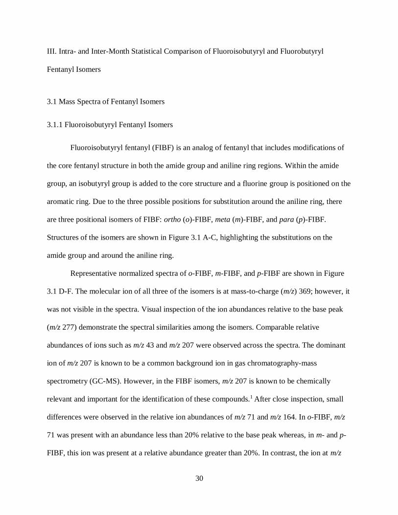
III. Intra- and Inter-Month Statistical Comparison of Fluoroisobutyryl and Fluorobutyryl

Fentanyl Isomers ....................................................................................................................... 30 3.1 Mass Spectra of Fentanyl Isomers.................................................................................... 30

3.1.1 Fluoroisobutyryl Fentanyl Isomers ............................................................................ 30 3.1.2 Fluorobutyryl Fentanyl Isomers ................................................................................ 32

3.2 Intra-Month Comparisons of FIBF and FBF Spectra to FIBF Reference Spectra .............. 34 3.2.1 Month 1 FIBF and FBF Spectra Compared to the Month 1 FIBF Reference Spectra . 35

3.2.2 Month 2 FIBF and FBF Spectra Compared to Month 2 FIBF Reference Spectra ....... 40 3.2.3 Month 3 FIBF and FBF Spectra Compared to Month 3 FIBF Reference Spectra ....... 44

3.2.4 Trends in the Month 1 – 3 Intra-Month Comparisons to FIBF Reference Spectra ...... 47 3.4 Inter-Month Comparisons of FIBF and FBF Spectra to FIBF Reference Spectra .............. 51

3.5 Summary ......................................................................................................................... 56 APPENDIX .............................................................................................................................. 58

REFERENCES ......................................................................................................................... 67

IV. Further Investigation of a Refined Approach to Predict Standard Deviation ........................ 69 4.1 Investigation of Regression Lines .................................................................................... 69

4.1.1 Testing for Outliers ................................................................................................... 70

vi

4.1.2 Investigating Different Linear Regions Within Each Plot .......................................... 73 4.2 Intra-Month Comparisons of FIBF and FBF Spectra to FIBF Reference Spectra Using the

Refined Method of Standard Deviation Prediction ................................................................. 76 4.2.1 Month 1 FIBF and FBF Spectra Compared to Month 1 FIBF Reference Spectra Using

the Refined Method to Predict Standard Deviation ............................................................ 77

4.2.2 Month 2 FIBF and FBF Spectra Compared to Month 2 FIBF Reference Spectra Using

the Refined Method to Predict Standard Deviation ............................................................ 85

4.2.3 Month 3 FIBF and FBF Spectra Compared to Month 3 FIBF Reference Spectra Using

the Refined Method to Predict Standard Deviation ........................................................... 88 4.4 Summary ......................................................................................................................... 92

APPENDIX .............................................................................................................................. 94 REFERENCES ....................................................................................................................... 115

V. Conclusions and Future Work............................................................................................. 117

5.1 Conclusions ................................................................................................................... 117 5.2 Future Work .................................................................................................................. 118

REFERENCES ....................................................................................................................... 121

vii

LIST OF TABLES

Table 3.1 Comparison of two FIBF comparison spectrum data collections in Month 1 (A and B)

to Month 1 FIBF reference mass spectra at the 99.9% confidence level ..................................... 36

Table 3.2 Comparison of Month 1 FBF comparison spectra to corresponding FIBF reference

spectra at the 99.9% confidence level ........................................................................................ 40

Table 3.3 Comparison of Month 2 FIBF comparison spectra and corresponding reference spectra

at the 99.9% confidence level .................................................................................................... 41




at the 99.9% confidence level .................................................................................................... 45



Table 3.7 Inter-month comparison of Month 1 FIBF as reference spectra and Month 2 FIBF as

comparison spectra at the 99.9% confidence level ..................................................................... 52

Table 3.8 Inter-month comparison of Month 1 FIBF as reference spectra and Month 2 FBF as


Table A3.1 PPMC coefficients of the pairwise comparisons of structural isomers of FIBF and

FBF ........................................................................................................................................... 58

Table A3.2 Comparison of two FIBF comparison spectrum data collections in Month 1 (A and

B) to Month 1 FBF reference mass spectra at the 99.9% confidence level ................................. 59

Table A3.3 Comparison of Month 1 FBF comparison spectra to corresponding FBF reference


Table A3.4 Comparison of Month 2 FIBF comparison spectra to corresponding Month 2 FBF

reference spectra at the 99.9% confidence level ......................................................................... 61

Table A3.5 Comparison of Month 2 FBF comparison spectra to corresponding Month 2 FBF




viii



Table A3.8 Inter-month comparison of Month 1 FBF as reference spectra and Month 2 FIBF as


Table A3.9 Inter-month comparison of Month 1 FBF as reference spectra and Month 2 FBF as


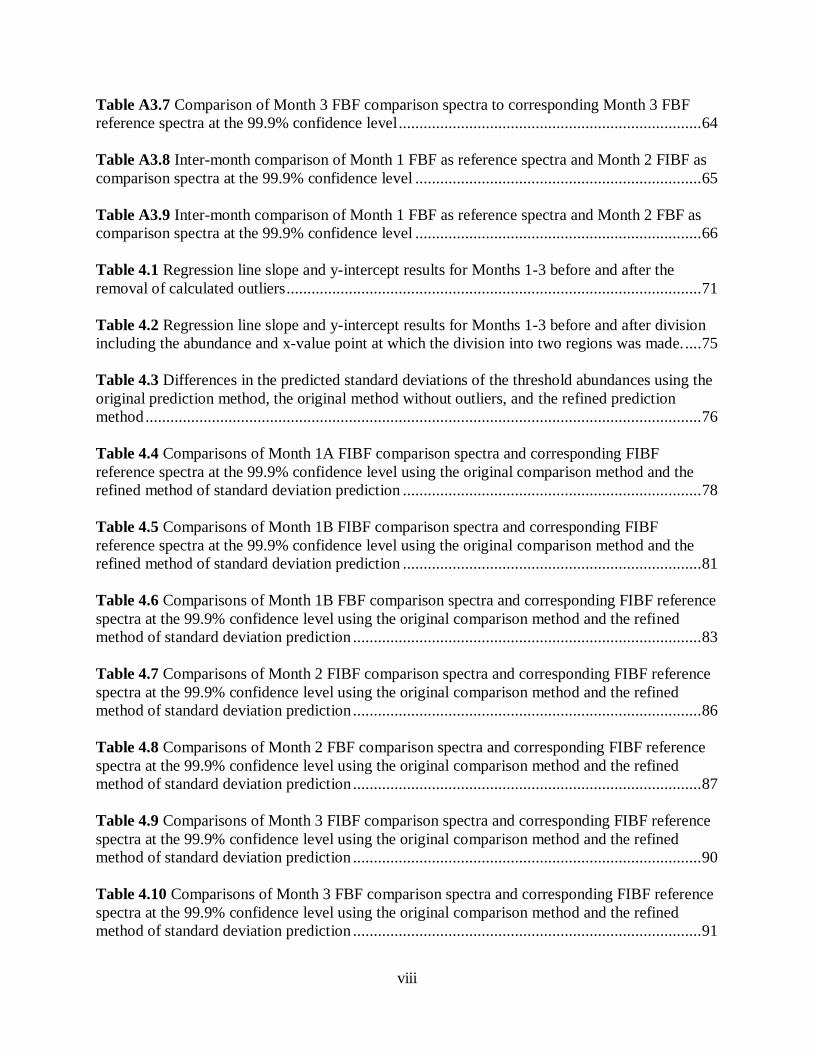
Table 4.1 Regression line slope and y-intercept results for Months 1-3 before and after the

removal of calculated outliers .................................................................................................... 71

Table 4.2 Regression line slope and y-intercept results for Months 1-3 before and after division

including the abundance and x-value point at which the division into two regions was made. .... 75

Table 4.3 Differences in the predicted standard deviations of the threshold abundances using the

original prediction method, the original method without outliers, and the refined prediction

method ...................................................................................................................................... 76

Table 4.4 Comparisons of Month 1A FIBF comparison spectra and corresponding FIBF

reference spectra at the 99.9% confidence level using the original comparison method and the

refined method of standard deviation prediction ........................................................................ 78

Table 4.5 Comparisons of Month 1B FIBF comparison spectra and corresponding FIBF


refined method of standard deviation prediction ........................................................................ 81

Table 4.6 Comparisons of Month 1B FBF comparison spectra and corresponding FIBF reference

spectra at the 99.9% confidence level using the original comparison method and the refined

method of standard deviation prediction .................................................................................... 83

Table 4.7 Comparisons of Month 2 FIBF comparison spectra and corresponding FIBF reference



Table 4.8 Comparisons of Month 2 FBF comparison spectra and corresponding FIBF reference









ix

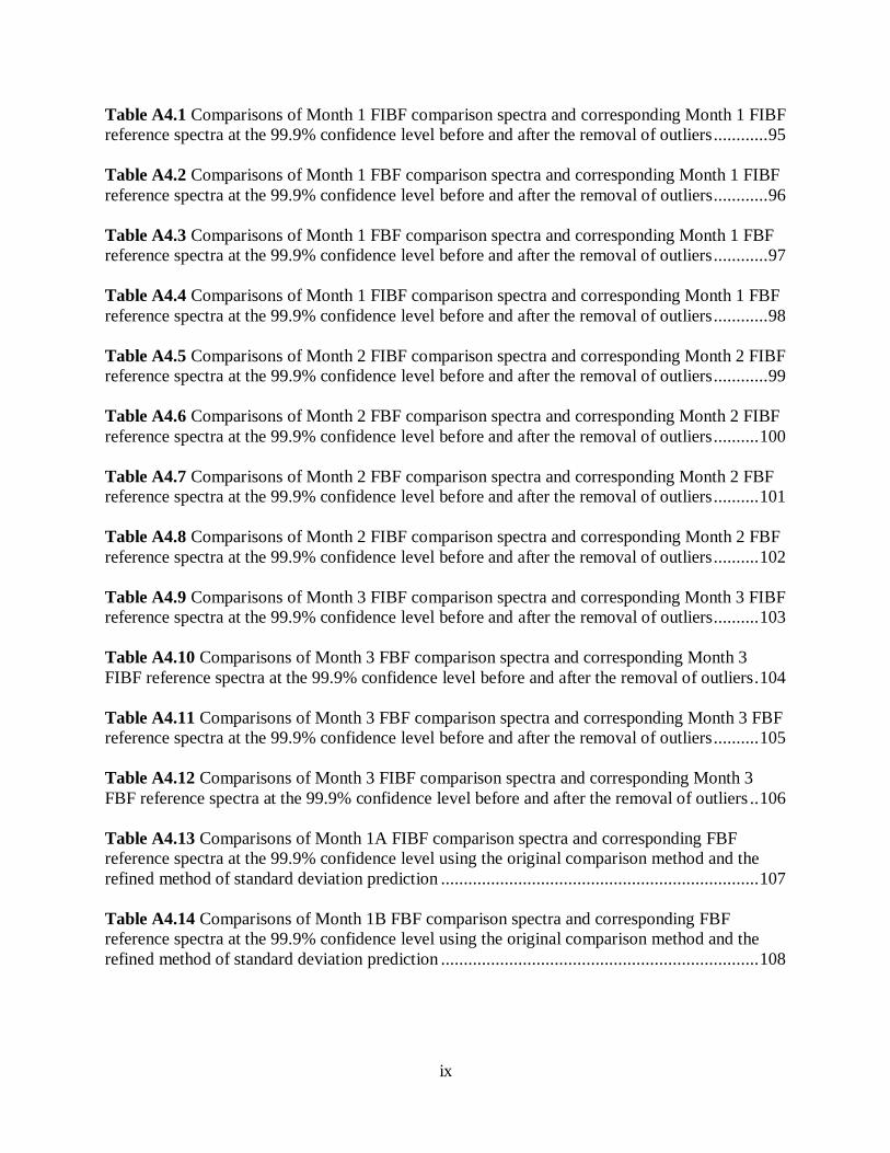
Table A4.1 Comparisons of Month 1 FIBF comparison spectra and corresponding Month 1 FIBF

reference spectra at the 99.9% confidence level before and after the removal of outliers ............ 95

Table A4.2 Comparisons of Month 1 FBF comparison spectra and corresponding Month 1 FIBF


Table A4.3 Comparisons of Month 1 FBF comparison spectra and corresponding Month 1 FBF


Table A4.4 Comparisons of Month 1 FIBF comparison spectra and corresponding Month 1 FBF





reference spectra at the 99.9% confidence level before and after the removal of outliers .......... 100







Table A4.10 Comparisons of Month 3 FBF comparison spectra and corresponding Month 3

FIBF reference spectra at the 99.9% confidence level before and after the removal of outliers. 104



Table A4.12 Comparisons of Month 3 FIBF comparison spectra and corresponding Month 3

FBF reference spectra at the 99.9% confidence level before and after the removal of outliers .. 106

Table A4.13 Comparisons of Month 1A FIBF comparison spectra and corresponding FBF


refined method of standard deviation prediction ...................................................................... 107

Table A4.14 Comparisons of Month 1B FBF comparison spectra and corresponding FBF



x

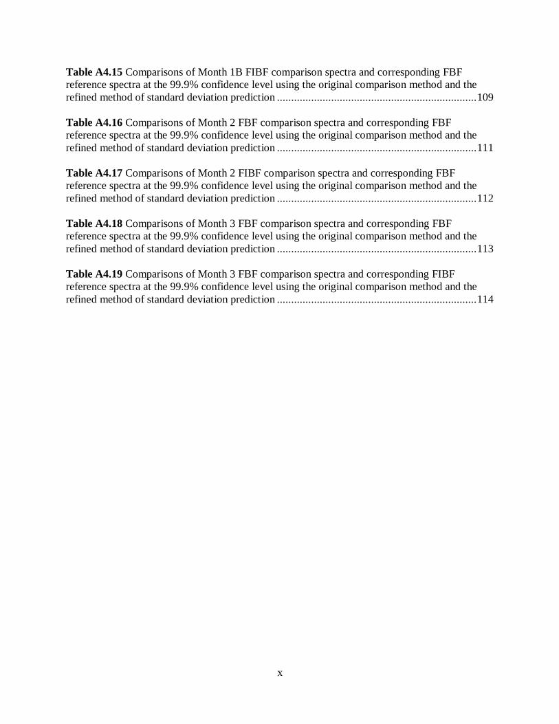
Table A4.15 Comparisons of Month 1B FIBF comparison spectra and corresponding FBF



Table A4.16 Comparisons of Month 2 FBF comparison spectra and corresponding FBF



Table A4.17 Comparisons of Month 2 FIBF comparison spectra and corresponding FBF






Table A4.19 Comparisons of Month 3 FBF comparison spectra and corresponding FIBF



xi

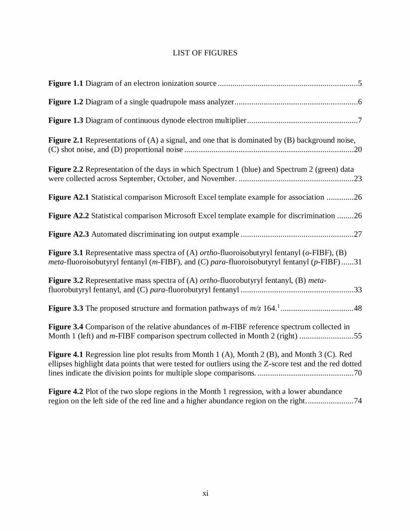
LIST OF FIGURES

Figure 1.1 Diagram of an electron ionization source ...................................................................5

Figure 1.2 Diagram of a single quadrupole mass analyzer...........................................................6

Figure 1.3 Diagram of continuous dynode electron multiplier .....................................................7

Figure 2.1 Representations of (A) a signal, and one that is dominated by (B) background noise,

(C) shot noise, and (D) proportional noise ................................................................................. 20

Figure 2.2 Representation of the days in which Spectrum 1 (blue) and Spectrum 2 (green) data

were collected across September, October, and November. ....................................................... 23

Figure A2.1 Statistical comparison Microsoft Excel template example for association ............. 26

Figure A2.2 Statistical comparison Microsoft Excel template example for discrimination ........ 26

Figure A2.3 Automated discriminating ion output example ...................................................... 27

Figure 3.1 Representative mass spectra of (A) ortho-fluoroisobutyryl fentanyl (o-FIBF), (B)

meta-fluoroisobutyryl fentanyl (m-FIBF), and (C) para-fluoroisobutyryl fentanyl (p-FIBF) ...... 31

Figure 3.2 Representative mass spectra of (A) ortho-fluorobutyryl fentanyl, (B) meta-

fluorobutyryl fentanyl, and (C) para-fluorobutyryl fentanyl ...................................................... 33

Figure 3.3 The proposed structure and formation pathways of m/z 164.1 ................................... 48

Figure 3.4 Comparison of the relative abundances of m-FIBF reference spectrum collected in

Month 1 (left) and m-FIBF comparison spectrum collected in Month 2 (right) .......................... 55

Figure 4.1 Regression line plot results from Month 1 (A), Month 2 (B), and Month 3 (C). Red

ellipses highlight data points that were tested for outliers using the Z-score test and the red dotted

lines indicate the division points for multiple slope comparisons. .............................................. 70

Figure 4.2 Plot of the two slope regions in the Month 1 regression, with a lower abundance

region on the left side of the red line and a higher abundance region on the right. ...................... 74

1

I. Introduction

1.1 Fentanyl Epidemic

Fentanyl is a Schedule II synthetic opioid that has medical applications as a pain killer

and as an anesthetic. This synthetic opioid is approximately 50 to 100 times more potent than

morphine and is known to provide a euphoric high and to be very addictive.1 Fentanyl was first

synthesized in 1960 and approved for medical use by the Food and Drug Administration (FDA)

in 1972. Very soon after its debut on the market, illicit fentanyl use began. In the late 1990s, the

FDA issued warnings about the use of the drug and recommended that it only be prescribed to

patients in a level of pain not managed by less potent opioids. The problem of illicit fentanyl use

has only grown in the 2000s, with a dramatic increase in 2013.2 According to the Drug

Enforcement Administration’s 2019 National Drug Threat Assessment, fentanyl is the main

contributor to the ongoing opioid crisis and is expected to remain a serious threat to the United

States in years to come.3

An additional problem to the growing fentanyl epidemic is that as soon as synthetic drugs

become regulated under the Controlled Substances Act, new analogs of the regulated compound

appear on the market. These analogs are synthesized to imitate the effects of the regulated

compounds, but are sufficiently different structurally to evade legal ramifications. This has led to

a fentanyl and fentanyl analog epidemic, with more than 77 fentanyl analogs classified as

Schedule I substances. In 2016, fentanyl surpassed heroin as the drug most often involved in

deadly overdoses. The number of deaths due to opioid overdoses involving fentanyl analogs

almost doubled between 2016 and 2017, with around 14 analogs observed the most often.

Among these main analogs are para-fluoroisobutyryl fentanyl (p-FIBF) and para-fluorobutyryl

2

fentanyl (p-FBF). These two compounds are positional isomers of each other and distinction of

isomers such as these can be challenging due to the high degree of structural similarity.2 This

research will focus on the two sets of positional isomers of FBF and FIBF.

Positional isomers are compounds that have the same core structure as well as the same

chemical formula and molecular weight.4 However, the difference is in the placement of the

functional group(s) on the compound. As an example, the three positional isomers of FIBF

(ortho-FIBF, meta-FIBF, and para-FIBF) have the same chemical formula of C23H29FN2O and

the same molecular weight of 368 atomic mass units (amu). The only difference is the position of

the fluorine substitution on the aniline ring – either in the ortho position, the meta position, or the

para position.5 Due to the high similarity in structure, it can be very difficult to distinguish

positional isomers using the typical instrumentation used in forensic laboratories for seized drug

identification.

1.2 Identification of Seized Drugs using Gas Chromatography-Mass Spectrometry

The Scientific Working Group for the Analysis of Seized Drugs (SWGDRUG) has

published recommendations for the identification of seized drugs.6 As part of the

recommendations, the analytical techniques typically used for identification are separated into

three categories: A, B, and C. These categories are used to create an analytical scheme to be

followed in order to ensure that the series of tests and techniques selected will offer enough

selectivity and specificity for accurate identification. Category A techniques provide the highest

level of selectivity through structural information. Such techniques include infrared (IR)

spectroscopy, nuclear magnetic resonance (NMR) spectroscopy, and mass spectrometry (MS).

When a Category A technique is used as part of the analytical scheme, only one other technique

from either Category A, B, or C is needed for identification. On the other hand, if a Category A

3

technique is not used, three different techniques must be used, with at least two of those

belonging to Category B which provides the second level of selectivity through chemical or

physical characteristics. The typical method for the identification of controlled substances is to

analyze samples with the use of a Category A technique (MS) coupled to a Category B

technique, gas chromatography (GC).

For GC-MS analysis, a submitted sample is dissolved in a suitable solvent and injected

into the GC. Following injection, the components of the sample are volatilized and separated via

GC, providing chemical characteristics, then go on to the MS to be ionized, providing structural

information. The results that are generated from this technique include a chromatogram with

retention time information and a mass spectrum with nominal mass information.

To identify the seized drug present in the submitted sample, a visual comparison of the

resulting mass spectrum to a suitable reference spectrum is conducted.6 The reference spectrum

may be a known standard analyzed on the same instrument under equivalent conditions or may

be a result from a reputable mass spectral library such as the National Institute of Standards and

Technology/Environmental Protection Agency/National Institutes of Health (NIST/EPA/NIH)

Mass Spectral library. While the National Academy of Sciences (NAS) deems the identification

of controlled substances to be a mature forensic discipline, there are some limitations to this

method of analysis.7 Identification is limited by the availability of pre-established mass spectral

libraries, which is even more difficult when identifying synthetic analogs as well as structural

and positional isomers. In addition, library search algorithms do not provide a measure of

statistical confidence in the identification, which is desired by the NAS. Currently, only a visual

assessment between the spectrum of the submitted sample and the reference spectrum is

4

conducted. And finally, the acceptance criteria to determine how similar the spectra are for an

identification may differ among laboratories and between cases.8

1.2.1 Gas Chromatography-Mass Spectrometry (GC-MS)

The most common technique for the identification of controlled substances is GC-MS. In

order to use the method, the submitted sample must be dissolved in a suitable solvent prior to the

injection into the GC. Following injection, the sample is vaporized into the gas phase and

separated into its various components using a capillary column coated with a liquid stationary

phase. An inert carrier gas propels the compounds through the column, and as they are separated

based on volatility and affinity to the stationary phase, the components elute from the column at

different times. Upon completion of separation via GC, the separated components move into the

mass spectrometer through a transfer line that is heated to keep the sample in the gas phase.9,10

There are three main components to the mass spectrometer: the ionization source, the

mass analyzer, and the detector. Once the separated components elute from the GC column, they

are ionized in the ion source of the mass spectrometer. While there are many different types of

ionization in MS, the most commonly used in seized drug analysis is electron ionization (EI),

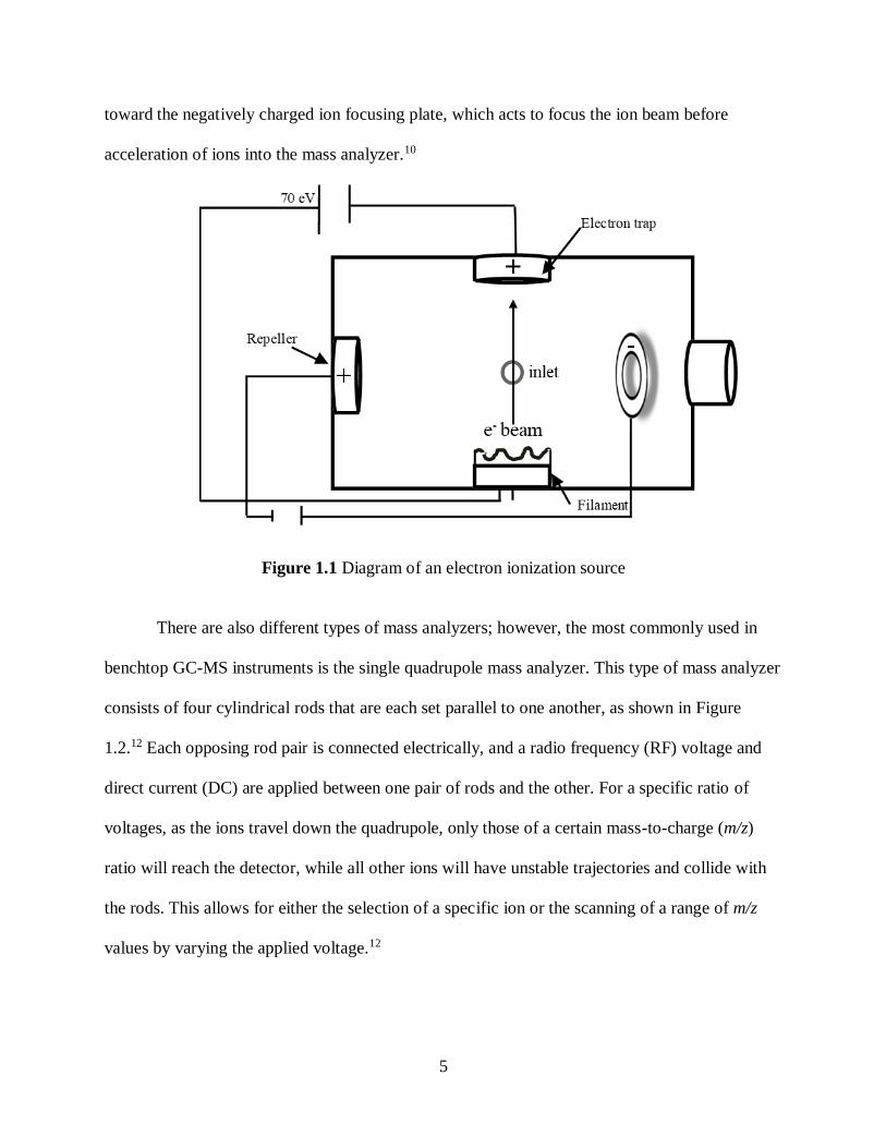
which is shown in Figure 1.1.10 Ionization through EI involves the bombardment of the sample

molecules with a high energy electron beam (70 eV). Produced by heating a wire filament with

an electric current, the beam is attracted to a positive charge at the opposite end of the ionization

chamber. The beam of electrons moves orthogonally to the transfer line and when the electrons

and the gas-phase molecules from the transfer line come into proximity with one another,

positive radical ions are formed.10 This is possible because the energy of the electron beam (70

eV) is sufficiently high to break the bonds of most organic compounds (4-20 eV).11 Following

the formation of the positive radical ions, the positively charged repeller electrode repels the ions

5

toward the negatively charged ion focusing plate, which acts to focus the ion beam before

acceleration of ions into the mass analyzer.10

Figure 1.1 Diagram of an electron ionization source

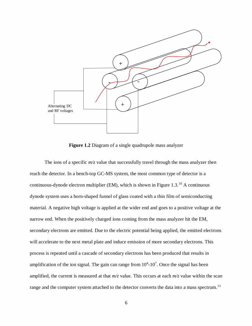
There are also different types of mass analyzers; however, the most commonly used in

benchtop GC-MS instruments is the single quadrupole mass analyzer. This type of mass analyzer

consists of four cylindrical rods that are each set parallel to one another, as shown in Figure

1.2.12 Each opposing rod pair is connected electrically, and a radio frequency (RF) voltage and

direct current (DC) are applied between one pair of rods and the other. For a specific ratio of

voltages, as the ions travel down the quadrupole, only those of a certain mass-to-charge (m/z)

ratio will reach the detector, while all other ions will have unstable trajectories and collide with

the rods. This allows for either the selection of a specific ion or the scanning of a range of m/z

values by varying the applied voltage.12

6

Figure 1.2 Diagram of a single quadrupole mass analyzer

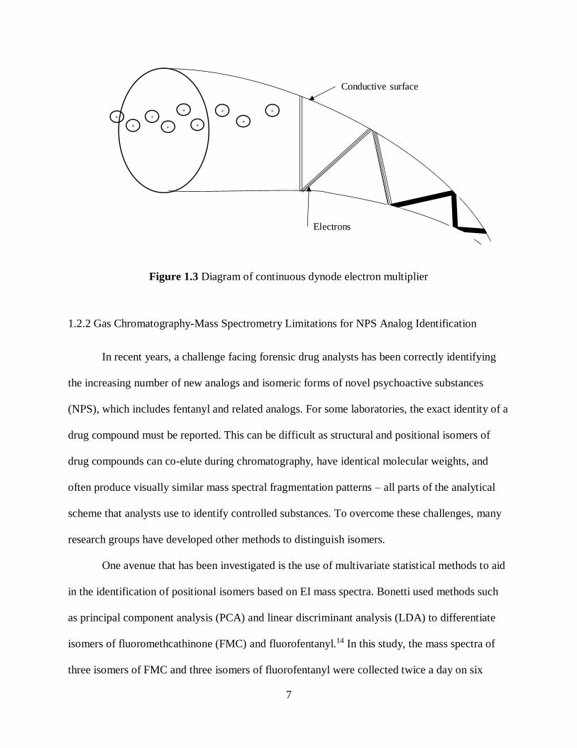
The ions of a specific m/z value that successfully travel through the mass analyzer then

reach the detector. In a bench-top GC-MS system, the most common type of detector is a

continuous-dynode electron multiplier (EM), which is shown in Figure 1.3.10 A continuous

dynode system uses a horn-shaped funnel of glass coated with a thin film of semiconducting

material. A negative high voltage is applied at the wider end and goes to a positive voltage at the

narrow end. When the positively charged ions coming from the mass analyzer hit the EM,

secondary electrons are emitted. Due to the electric potential being applied, the emitted electrons

will accelerate to the next metal plate and induce emission of more secondary electrons. This

process is repeated until a cascade of secondary electrons has been produced that results in

amplification of the ion signal. The gain can range from 104-107. Once the signal has been

amplified, the current is measured at that m/z value. This occurs at each m/z value within the scan

range and the computer system attached to the detector converts the data into a mass spectrum.13

+

+

-

Alternating DC

and RF voltages

-

7

Figure 1.3 Diagram of continuous dynode electron multiplier

1.2.2 Gas Chromatography-Mass Spectrometry Limitations for NPS Analog Identification

In recent years, a challenge facing forensic drug analysts has been correctly identifying

the increasing number of new analogs and isomeric forms of novel psychoactive substances

(NPS), which includes fentanyl and related analogs. For some laboratories, the exact identity of a

drug compound must be reported. This can be difficult as structural and positional isomers of

drug compounds can co-elute during chromatography, have identical molecular weights, and

often produce visually similar mass spectral fragmentation patterns – all parts of the analytical

scheme that analysts use to identify controlled substances. To overcome these challenges, many

research groups have developed other methods to distinguish isomers.

One avenue that has been investigated is the use of multivariate statistical methods to aid

in the identification of positional isomers based on EI mass spectra. Bonetti used methods such

as principal component analysis (PCA) and linear discriminant analysis (LDA) to differentiate

isomers of fluoromethcathinone (FMC) and fluorofentanyl.14 In this study, the mass spectra of

three isomers of FMC and three isomers of fluorofentanyl were collected twice a day on six

++

+

+

++

++

+

Conductive surface

Electrons

8

instruments over five days. An additional nineteen blind samples were also included. Visual

inspection of the LDA plots was paired with objective classifications using posterior

probabilities generated during LDA. Bonetti’s conclusion was that the use of multivariate

statistics is a feasible way to highlight small but reproducible differences in the mass spectra of

positional isomers for identification purposes.14

In another study using multivariate statistics, Davidson and Jackson differentiated

positional isomers of 1,5-dimethoxy-N-(N-methoxybenzyl)phenethylamines (NBOMes).15 The

isomers were differentiated based on retention indices and ion ratios of only the fifteen most

abundant ions in the spectra using PCA and LDA. In conclusion, the LDA classification was

99.5% accurate across different instruments and was 99.9% accurate when using the same

instrument.14 While both of the studies from Bonetti and Davidson and Jackson provide very

useful methods to identify and differentiate positional isomers using GC-MS, the methods

required the use of several instruments and different compounds to develop the robust training

sets necessary to perform multivariate statistical analysis. This can be very time-consuming and

difficult in a forensic laboratory setting.14,15

Other methods to distinguish positional isomers include the use of different GC detectors

rather than, or in addition to, MS. Kranenburg et al. reported the use of vacuum-ultraviolet

spectroscopy (VUV) as a detector for GC to differentiate isomers of phenethylamines and

cathinones.16 The GC-VUV system provided spectra with distinct differences for positional

isomers of substituents on aromatic rings. Although the VUV spectra of some classes of drug

compounds appeared visually similar, small differences were enough to differentiate isomers

because of the robustness and reproducibility of the spectral data.16

9

Other methods for positional isomer differentiation include modifications to the

ionization method, which is generally EI. One such modification, reported by Kranenburg et al.

is low-energy EI, which can lead to changes in intensity ratio patterns which affect each

positional isomer differently.17 Using an ionization energy of 15 eV (rather than the more

conventional 70 eV), mass spectra of cathinone isomers were distinguished with the aid of PCA

and LDA. The accuracy of this method was demonstrated with 100% correct isomer

identification of six forensic case samples.17

Another modification to the ionization method which was reported by Buchalter et al.

was the use of GC with tandem cold EI-MS and VUV detection.18 Cold EI-MS is based on

cooling the molecules as they are transported from the GC into the mass spectrometer. Reducing

the temperature of the molecules enhanced the survival of the ions during ionization. The study

investigated the efficacy of the tandem detection system for the analysis of twenty-four fentanyl

analogs, including seven sets of positional isomers. In conclusion, the combination of GC in

tandem with cold EI-MS and VUV was determined to result in higher confidence in sample

identification using retention time and mass spectra that included larger relative intensities of the

molecular ion. While the positional isomers were found to produce very similar mass spectra

even with cold EI-MS, the VUV spectra were unique enough for distinguishability in this case.

While the methods presented by Kranenburg et al. and Buchalter et al. did allow for the

distinction of isomers, the instrumentation is not widely available in forensic laboratories and

would be expensive to institute.16,17,18

10

1.3 Statistical Comparison Method

To address limitations in positional isomer differentiation, Willard et al. developed a

statistical method to compare the mass spectrum of an unknown sample to that of a reference

material using an unequal variance t-test.8,19 In this approach, t-tests are used to statistically

compare the mean abundances at every corresponding m/z value in the two spectra. The null (H0)

and alternative (Ha) hypotheses are shown below in Equations 1.1 and 1.2, respectively

𝐻0 : |�̅�1𝑗 − �̅�2𝑗| = 0 (1.1)

𝐻𝑎 : |�̅�1𝑗 − �̅�2𝑗| ≠ 0 (1.2)

where �̅�1𝑗 and �̅�2𝑗 are the mean abundances of ion j in spectra 1 and 2. The hypotheses are tested

using the Welch’s t-test calculation (tcalc) as shown in Equation 1.3

𝑡calc = |�̅�1−�̅�2|

√𝑠1

2

𝑛1 −

𝑠22

𝑛2

(1.3)

where �̅�1and �̅�2 are the mean abundances at a common m/z ratio for the two spectra and n1 and n2

are the number of spectra used to calculate the standard deviations (s1 and s2) of the mean

abundances. The degrees of freedom calculation for the t-test is shown in Equation 1.4

𝑣 =(

𝑠12

𝑛1 −

𝑠22

𝑛2)

1

𝑛1−1(

𝑠12

𝑛1)

2

+ 1

𝑛2−1(

𝑠22

𝑛2)

2 (1.4)

In order to perform the t-test, a critical t-value is determined using the appropriate statistical table

according to the degrees of freedom which were calculated and the user-specified confidence

level. The calculated t-value is then compared to the corresponding critical t-value. If H0 is

accepted at every m/z value, the two spectra are determined to be statistically indistinguishable,

at the confidence level specified by the user when performing the t-test. However, if Ha is

accepted at any m/z value, then the two spectra are determined to be statistically distinguishable.

11

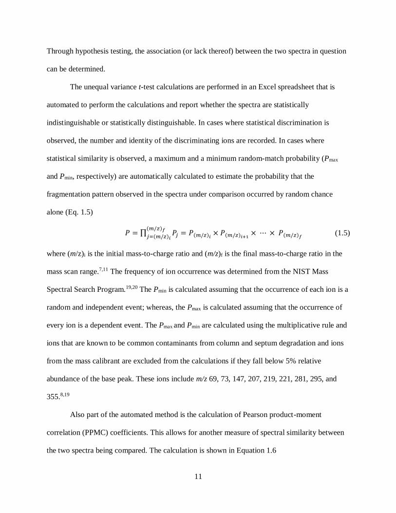
Through hypothesis testing, the association (or lack thereof) between the two spectra in question

can be determined.

The unequal variance t-test calculations are performed in an Excel spreadsheet that is

automated to perform the calculations and report whether the spectra are statistically

indistinguishable or statistically distinguishable. In cases where statistical discrimination is

observed, the number and identity of the discriminating ions are recorded. In cases where

statistical similarity is observed, a maximum and a minimum random-match probability (Pmax

and Pmin, respectively) are automatically calculated to estimate the probability that the

fragmentation pattern observed in the spectra under comparison occurred by random chance

alone (Eq. 1.5)

𝑃 = ∏ 𝑃𝑗 = 𝑃(𝑚/𝑧)𝑖× 𝑃(𝑚/𝑧)𝑖+1

× ⋯ × 𝑃(𝑚/𝑧)𝑓

(𝑚/𝑧)𝑓

𝑗=(𝑚/𝑧)𝑖 (1.5)

where (m/z)i is the initial mass-to-charge ratio and (m/z)f is the final mass-to-charge ratio in the

mass scan range.7,11 The frequency of ion occurrence was determined from the NIST Mass

Spectral Search Program.19,20 The Pmin is calculated assuming that the occurrence of each ion is a

random and independent event; whereas, the Pmax is calculated assuming that the occurrence of

every ion is a dependent event. The Pmax and Pmin are calculated using the multiplicative rule and

ions that are known to be common contaminants from column and septum degradation and ions

from the mass calibrant are excluded from the calculations if they fall below 5% relative

abundance of the base peak. These ions include m/z 69, 73, 147, 207, 219, 221, 281, 295, and

355.8,19

Also part of the automated method is the calculation of Pearson product-moment

correlation (PPMC) coefficients. This allows for another measure of spectral similarity between

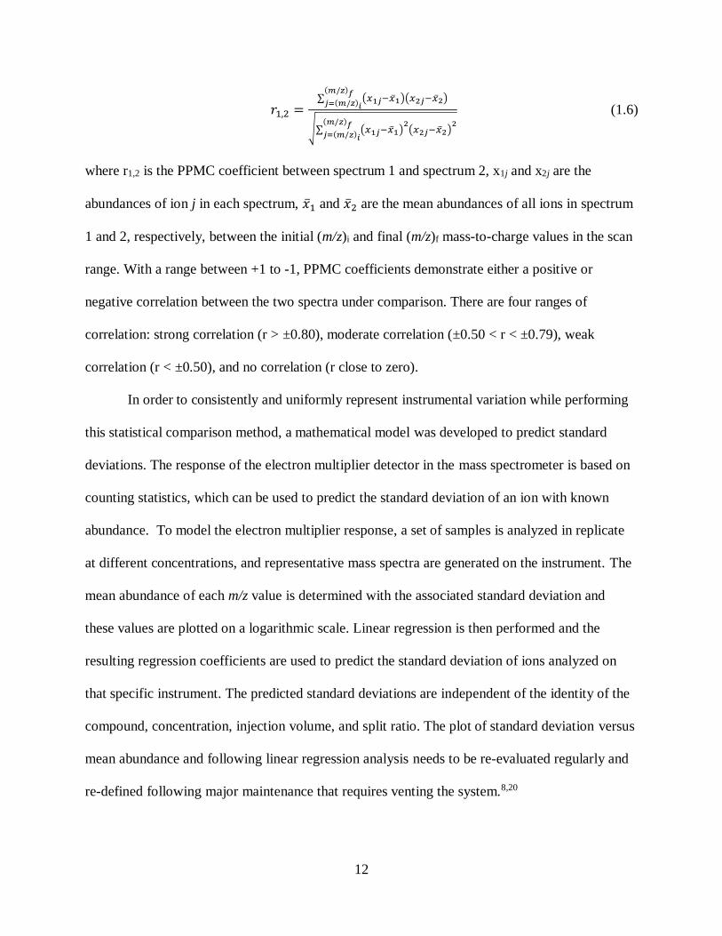
the two spectra being compared. The calculation is shown in Equation 1.6

12

𝑟1,2 =∑ (𝑥1𝑗−�̅�1)(𝑥2𝑗−�̅�2)

(𝑚/𝑧)𝑓𝑗=(𝑚/𝑧)𝑖

√∑ (𝑥1𝑗−�̅�1)2

(𝑥2𝑗−�̅�2)2(𝑚/𝑧)𝑓

𝑗=(𝑚/𝑧)𝑖

(1.6)

where r1,2 is the PPMC coefficient between spectrum 1 and spectrum 2, x1j and x2j are the

abundances of ion j in each spectrum, �̅�1 and �̅�2 are the mean abundances of all ions in spectrum

1 and 2, respectively, between the initial (m/z)i and final (m/z)f mass-to-charge values in the scan

range. With a range between +1 to -1, PPMC coefficients demonstrate either a positive or

negative correlation between the two spectra under comparison. There are four ranges of

correlation: strong correlation (r > ±0.80), moderate correlation (±0.50 < r < ±0.79), weak

correlation (r < ±0.50), and no correlation (r close to zero).

In order to consistently and uniformly represent instrumental variation while performing

this statistical comparison method, a mathematical model was developed to predict standard

deviations. The response of the electron multiplier detector in the mass spectrometer is based on

counting statistics, which can be used to predict the standard deviation of an ion with known

abundance. To model the electron multiplier response, a set of samples is analyzed in replicate

at different concentrations, and representative mass spectra are generated on the instrument. The

mean abundance of each m/z value is determined with the associated standard deviation and

these values are plotted on a logarithmic scale. Linear regression is then performed and the

resulting regression coefficients are used to predict the standard deviation of ions analyzed on

that specific instrument. The predicted standard deviations are independent of the identity of the

compound, concentration, injection volume, and split ratio. The plot of standard deviation versus

mean abundance and following linear regression analysis needs to be re-evaluated regularly and

re-defined following major maintenance that requires venting the system.8,20

13

1.3.1 Previous Applications of the Statistical Comparison Method

The statistical comparison method was developed and validated for a set of normal

alkanes and has been applied for the differentiation of amphetamine-type stimulants and

salvinorins extracted from the plant material, Salvia divinorum.8,19,20,21 More recently,

application of the method to successfully discriminate positional isomers of

fluoromethamphetamine and ethylmethcathinone has been demonstrated,22 along with an initial

investigation into the effects of instrument parameters (tune and split ratio) on the statistical

association and discrimination of isomers.23 In this study, spectra were collected on consecutive

days and then about a month apart to be compared and successful association and discrimination

of the positional isomers was generally observed. In addition to the research involving statistical

comparisons of various samples, the method used to predict standard deviation based on electron

multiplier counting statistics was further investigated. Typically, a linear regression plot of

standard deviation and mean abundance is used; however, during the investigation, it appeared

that there were two separate linear regions that could be used.

1.4 Research Objectives

The main objective in this research was to investigate the robustness of the previously

developed statistical comparison method for differentiation of positional isomers. To achieve this

objective, two sets of fentanyl isomers (FIBF and FBF) were analyzed on the same instrument

under equivalent conditions. With the chosen sets of fentanyl isomers being not only positional

isomers, but also structural isomers of one another, the ability of the method to differentiate was

tested in ways not previously investigated. As mass spectral data were collected for each isomer,

the robustness of the method was further assessed by comparing spectra collected across a three-

month time period. During this relatively short time study, the effects of major instrument

14

maintenance (involving venting of the system) as well as high instrument usage (involving other

research groups using the same instrument for other purposes) on the ability to maintain proper

association and discrimination of the fentanyl isomers were investigated.

In addition, the method to predict standard deviation based on the electron multiplier

response was further refined. Previous research investigated the possibility of two linear regions

within the regression instead of just one region. In this work, following comparisons that resulted

in inaccurate association and discrimination of isomers, the method to predict standard deviation

utilizing two linear regions of the regression was tested. The effect of the refined method on the

ability to successfully associate and discriminate the isomers was then investigated.

By applying the statistical comparison method to a new set of both structural and

positional isomers, the robustness of the method for the use of isomer and analog differentiation

will be further investigated and the accuracy to which isomers are successfully associated and

discriminated will be determined. Following the refinement of the method to more accurately

predict the standard deviations, this method of positional isomer differentiation can be compared

to additional methods for use in forensic science laboratories.

15

REFERENCES

16

REFERENCES

(1) Centers for Disease Control and Prevention. Drugs Most Frequently Involved in Drug

Overdose Deaths: United States, 2011-2016. National Vital Statistics Reports. 2018, 67 (9),

1-13.

(2) Armenian, P.; Vo, K. T.; Barr-Walker, J.; Lynch, K. L. Fentanyl, fentanyl analogs and novel

synthetic opioids: A comprehensive review. Neuropharmacology. 2017, 1-13.

(3) Drug Enforcement Administration. National Drug Threat Assessment; Washington, D.C.:

U.S. Department of Justice, Drug Enforcement Administration, 2019.

(4) Merriam Webster. Position Isomerism. https://www.merriam-

webster.com/dictionary/positionisomerism (accessed 08/14/20).

(5) Cayman Chemical Company. Product Information; Ann Arbor, MI. 07/05/2019.

(6) Scientific Working Group for the Analysis of Seized Drugs. Recommendations; U.S

Department of Justice, Drug Enforcement Administration: Washington, DC, 2019; Vol. 8.0.

(7) National Research Council. Strengthening Forensic Science in the United States: A Path

Forward. Washington, DC: The National Academies Press. 2009.

(8) Bodnar Willard, M. A. Development and Application of a Statistical Approach to Establish

Equivalence of Unabbreviated Mass Spectra. Ph.D., Michigan State, 2013.

(9) Skoog, D.; West, D.; Holler, F. J. Fundamentals of Analytical Chemistry, 5th Edition, 5th ed.;

Saunders College; United States, 1988.

(10) Hoffmann, E. de; Stroobant, V. Mass Spectrometry: Principles and Applications, 3rd ed.;

Wiley; Chichester, 2007.

(11) Kellogg, M. D. Chapter 8 – Measurement of Biological Materials A2 – Robertson, D. In

Clinical and Translational Science (Second Edition); Williams, G. H., Ed.; Academic Press,

2017; pp 137-155.

(12) Harris, D. C. Exploring Chemical Analysis; W. H. Freeman: New York, 2013.

(13) Watson, J. T.; Sparkman, O. D. Introduction to Mass Spectrometry: Instrumentation,

Applications and Strategies for Data Interpretation, 4th ed.; John Wiley & Sons: Hoboken,

2007.

https://www.merriam-webster.com/dictionary/positionisomerism

https://www.merriam-webster.com/dictionary/positionisomerism

17

(14) Bonetti, J. Mass Spectral Differentiation of Positional Isomers Using Multivariate Statistics.

Forensic Chemistry 2018, 9, 50–61. https://doi.org/10.1016/j.forc.2018.06.001.

(15) Davidson, J. T.; Jackson, G. P. The Differentiation of 2,5-Dimethoxy-N-(N-

Methoxybenzyl)Phenethylamine (NBOMe) Isomers Using GC Retention Indices and

Multivariate Analysis of Ion Abundances in Electron Ionization Mass Spectra. Forensic

Chemistry 2019, 14, 100160. https://doi.org/10.1016/j.forc.2019.100160.

(16) Kranenburg, R. F.; Garcia-Cicourel, A. R.; Kukurin, C.; Janssen, H. G.; Schoenmakers, P.

J.; van Asten, A. C. Distinguishing drug isomers in the forensic laboratory: GC-VUV in

addition to GC-MS for orthogonal selectivity and the use of library match scores as a new

source of information. Forensic Science International 2019, 302

(17) Kranenburg, R. F.; Peroni, D.; Affourtit, S.; Westerhuis, J. A.; Smilde, A. K.; van Asten, A.

C. Revealing hidden information in GC-MS spectra from isomeric drugs: Chemometrics

based identification from 15 eV and 70 eV EI mass spectra. Forensic Chemistry, 2020, 18

(18) Buchalter, S.; Marginean, I.; Yohannan, J.; Lurie, I. S. Gas chromatography with tandem

cold electron ionization mass spectrometric detection and vacuum ultra-violet detection for

the comprehensive analysis of fentanyl analogues. Journal of Chromatography A 2019

(19) Bodnar Willard, M. A.: Waddell Smith, R.; McGuffin, V. L. Statistical approach to establish

equivalence of unabbreviated mass spectra. Rapid Communications in Mass Spectrometry

2013; 28(1):83–95.

(20) Bodnar Willard, M. A.; McGuffin V. L.; Waddell Smith, R. Statistical Comparison of Mass

Spectra for Identification of Amphetamine-Type Stimulants. Forensic Science International

270 2017; 111-20.

(21) Bodner Willard, M. A.; Hurd, J. E.; Waddell Smith, R.; McGuffin, V. L. Statistical

comparison of mass spectra of salvinorins in Salvia divinorum and related Salvia species.

Forensic Chemistry 17, 2020, 100192.

(22) Stuhmer, E. L.; McGuffin, V. L.; Waddell Smith, R.; Discrimination of seized drug

positional isomers based on statistical comparison of electron-ionization mass spectra.

Forensic Chemistry 20, 2020, 100261.

(23) Stuhmer, E. Statistical Comparison of Mass Spectral Data for Positional Isomer

Differentiation, M.S., Michigan State University, 2019.

18

II. Materials and Methods

2.1 Preparation of Fentanyl Analog and Isomer Solutions

The ortho-, meta-, and para- isomers of fluoroisobutyryl fentanyl (FIBF) and ortho-,

meta-, and para- isomers of fluorobutyryl fentanyl (FBF) were purchased from Cayman

Chemical (Ann Arbor, MI). Each compound was prepared at 1 mg/mL in methanol (ACS Grade,

Sigma Aldrich, St. Louis, MO) prior to analysis.

2.2 Gas Chromatography-Electron Ionization-Mass Spectrometry Analysis

Each isomer was analyzed using an Agilent 7890A gas chromatograph coupled to an

Agilent 5975c mass spectrometer with triple axis detector and a CTC-PAL autosampler (CTC

Analytics, Zwingen, Switzerland). The carrier gas was ultra-high purity helium (Airgas,

Independence, OH) at a nominal flow rate of 1 mL/min. An inert GC capillary column was used

with a 5% diphenyl-95% dimethylpolysiloxane stationary phase (VF-5ms, 30 m x 0.25 mm x

0.25 µm, Agilent Technologies).

Each isomer was analyzed over a three-month time period under two scenarios – to be

used as the reference spectrum, which would typically be considered the reference standard in a

forensic laboratory, and to be used as the comparison spectrum, or case sample if the method is

applied to real casework. In the case of the reference spectrum analysis, each isomer was

analyzed in replicate (n = 5) and in the case of the comparison spectrum analysis, each of the six

isomers was analyzed once. One exception was during the first month collection, where only the

three FIBF isomers were analyzed for comparison spectra and analysis was performed in

replicate (n=3).

Each isomer was injected onto the instrument (1 µL) at a split ratio of 100:1 for each day

of reference and comparison spectra data collection. Samples were all analyzed under equivalent

19

conditions based on the following parameters. The injector port temperature was 220 °C and the

oven temperature program was as follows: 200 °C for 1 min, 30 °C/min to 300 °C, with a final

hold of 8 min. The transfer line was maintained at 300 °C and the mass spectrometer was

operated in electron ionization mode (70 eV), with a scan range of m/z 40-450 and a scan rate of

4.51 scans/s.

2.3 Predicted Standard Deviation

In order to perform unequal variance t-tests at each m/z value between two mass spectra,

the mean abundance and standard deviation of each abundance at every m/z value must be

calculated (Equations 1.3 and 1.4, Section 1.3). Instead of calculating the mean abundance and

standard deviation using replicates, the standard deviation can be predicted based on the counting

statistics of the electron multiplier detector in the GC-MS. This method also allows for a

consistent and uniform representation of instrumental variation while performing the statistical

comparison method.

2.3.1 Modeling the Electron Multiplier Response

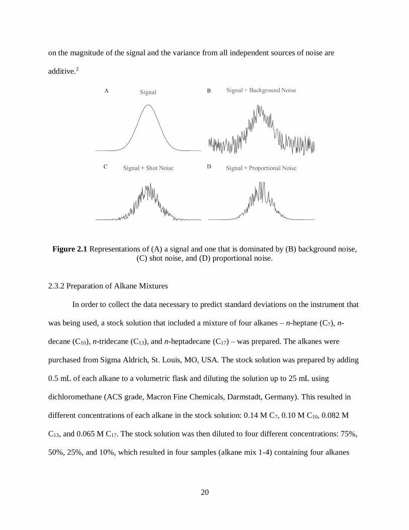
There are three different sources of noise in electron multipliers: background noise, shot

noise, and proportional noise.1 Representations of a signal dominated by each source of noise is

shown in Figure 2.1. Background noise is constant and can be caused by a multitude of sources

including the carrier gas and column from the gas chromatograph or even a vacuum leak in the

mass spectrometer. Shot noise is caused by the randomness in the number of electrons that are

multiplied throughout the continuous dynode. Each electron that strikes the dynodes results in a

random three to 6 electrons multiplied. Shot noise is proportional to the square root of the signal.

Proportional noise scales directly with the signal. The total noise which is observed for any given

signal is from a combination of all three sources. The variances of each source of noise depend

20

on the magnitude of the signal and the variance from all independent sources of noise are

additive.2

Figure 2.1 Representations of (A) a signal and one that is dominated by (B) background noise,

(C) shot noise, and (D) proportional noise.

2.3.2 Preparation of Alkane Mixtures

In order to collect the data necessary to predict standard deviations on the instrument that

was being used, a stock solution that included a mixture of four alkanes – n-heptane (C7), n-

decane (C10), n-tridecane (C13), and n-heptadecane (C17) – was prepared. The alkanes were

purchased from Sigma Aldrich, St. Louis, MO, USA. The stock solution was prepared by adding

0.5 mL of each alkane to a volumetric flask and diluting the solution up to 25 mL using

dichloromethane (ACS grade, Macron Fine Chemicals, Darmstadt, Germany). This resulted in

different concentrations of each alkane in the stock solution: 0.14 M C7, 0.10 M C10, 0.082 M

C13, and 0.065 M C17. The stock solution was then diluted to four different concentrations: 75%,

50%, 25%, and 10%, which resulted in four samples (alkane mix 1-4) containing four alkanes

21

each. This preparation process was repeated as necessary during the three months of data

collection.

All four samples of the alkane mix were analyzed on the same GC-MS instrument in

triplicate using parameters described by the National Center for Forensic Science. Each sample

was injected with a volume of 1 µL at a 50:1 split ratio. The injector port temperature was

maintained at 250 °C and the oven temperature program was as follows: initial temperature 50

°C held for 3 min, 10 °C/min to 280 °C, with a final hold of 4 min. The transfer line was

maintained at 280 °C and the mass spectrometer was operated in electron ionization mode (70

eV), with a scan range of m/z 40 – 450, and a scan rate of 4.59 scans/s. Spectra were collected for

each alkane in each concentration mixture for every replicate yielding a total of 48 spectra. This

procedure was repeated each time major maintenance requiring venting of the instrument (e.g.,

changing the column or cleaning the ion source) was performed.

2.3.3 Generation of Standard Deviation Plot

After data collection (48 total spectra), the mean abundances of the spectra collected at

the apex of the chromatographic peak and the associated standard deviations for the replicates of

each alkane at each concentration were calculated. A logarithmic plot of the standard deviation

versus mean abundance was generated and linear regression analysis was performed in Microsoft

Excel (version 12.0, Microsoft Corporation, Redmond, WA). The resulting slope and y-intercept

from the regression equation were used to determine the predicted standard deviation of

compounds analyzed on that specific instrument under equivalent conditions as long as the

abundance of all ions are known. The predicted standard deviations are independent of the

identity of the compound, concentration, injection volume, and split ratio, but are not

22

independent of instrument. Therefore, separate plots must be produced if analyzing samples on

different instruments and after venting of the system.

Due to the rigorous use of the Agilent instrument used for this research and the number of

column changes during the duration of this research, a new regression plot was required for each

month’s analysis. Using a procedure to statistically compare the slopes of two regression lines

detailed by Andrade and Estévez-Pérez, the slopes of each regression line were statistically

compared on a month-to-month basis.3

2.4 Data Analysis

Representative mass spectra for the FIBF and FBF isomers were collected at the apex of

the corresponding chromatographic peak (100% relative abundance). The data were exported

into a CSV file from ChemStation (version #E.02.01.1177, Agilent Technologies) and

transferred to a Microsoft Excel worksheet that is used to automate the previously developed

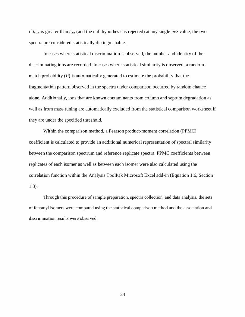
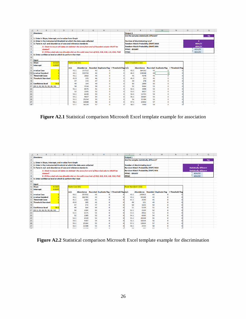
statistical comparison method (Appendix Tables A2.1 – 2.3).4,5

The arrangement of the statistical comparison worksheet allows for the comparison of a

single mass spectrum, the comparison spectrum in this case, to three replicate spectra, the

reference spectra in this case. Mass spectral data for each isomer were collected across three

consecutive months (September – November), which will be referred to as Month 1, Month 2,

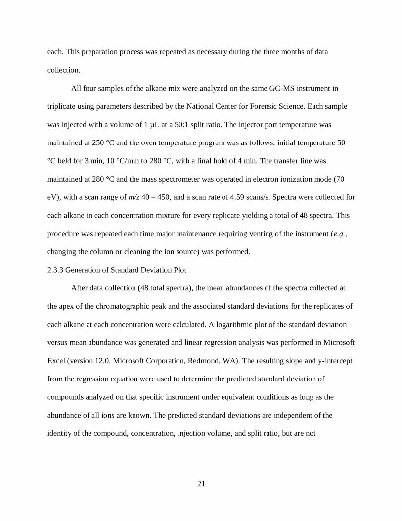
and Month 3. The specific days in which the samples were analyzed are shown in Figure 2.1.

During Month 1, comparison spectra were collected twice (A and B) to observe the differences

and similarities in the comparison results within the same month of data collection. Month 1A

comparison spectra only included the three FIBF samples, whereas the Month 1B collection

included all six isomers. In addition, reference spectra for the FBF compounds were collected on

a separate day than the reference spectra for the FIBF compounds. This was the case for each

23

month due to time constraints. During Month 2 and Month 3, comparison spectra were collected

once for all six isomers and the reference spectra were collected in triplicate on a separate day.

Collecting data in this manner ensured that comparisons were between spectra collected on

different days, rather than comparisons of instrument replicates.

Figure 2.2 Representation of the days in which Spectrum 1 (blue) and Spectrum 2

(green) data were collected across September, October, and November.

Once the raw mass spectral data were transferred into the Excel worksheet, the template

automatically zero-filled and normalized the spectral data to ensure an abundance was given at

each m/z value in the defined scan range of m/z 40-400 and that relative abundances could be

statistically compared. The comparison worksheet was also automated to round each m/z value to

the nearest whole number and to flag any duplicates. If two m/z values round to the same whole

number, the second abundance is always used unless action is taken by the analyst. Within the

worksheet, statistical comparisons were made by performing an unequal variance t-test at each

m/z value in the scan range. These calculations were also automated by the worksheet and use

the predicted standard deviation procedure discussed in Section 2.3. Taking the results of the t-

test, the calculated t-values (tcalc) were compared to the critical t-values (tcrit) at each m/z value to

determine the statistical similarity or dissimilarity of the two spectra under comparison. If tcalc is

determined to be less than or equal to tcrit (and the null hypothesis is accepted) at every single

ion, the two spectra being compared are considered statistically similar to one another. However,

Reference

Comparison

24

if tcalc is greater than tcrit (and the null hypothesis is rejected) at any single m/z value, the two

spectra are considered statistically distinguishable.

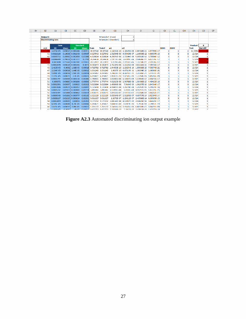
In cases where statistical discrimination is observed, the number and identity of the

discriminating ions are recorded. In cases where statistical similarity is observed, a random-

match probability (P) is automatically generated to estimate the probability that the

fragmentation pattern observed in the spectra under comparison occurred by random chance

alone. Additionally, ions that are known contaminants from column and septum degradation as

well as from mass tuning are automatically excluded from the statistical comparison worksheet if

they are under the specified threshold.

Within the comparison method, a Pearson product-moment correlation (PPMC)

coefficient is calculated to provide an additional numerical representation of spectral similarity

between the comparison spectrum and reference replicate spectra. PPMC coefficients between

replicates of each isomer as well as between each isomer were also calculated using the

correlation function within the Analysis ToolPak Microsoft Excel add-in (Equation 1.6, Section

1.3).

Through this procedure of sample preparation, spectra collection, and data analysis, the sets

of fentanyl isomers were compared using the statistical comparison method and the association and

discrimination results were observed.

25

APPENDIX

26

Figure A2.1 Statistical comparison Microsoft Excel template example for association

Figure A2.2 Statistical comparison Microsoft Excel template example for discrimination

27

Figure A2.3 Automated discriminating ion output example

28

REFERENCES

29

REFERENCES

(1) Shockley, W.; Pierce, J. R. A Theory of Noise for Electron Multipliers. Proceedings of the

Institute of Radio Engineers 1938, 26 (3), 321-332.

(2) O’Haver, T. Signals and Noise. A Pragmatic Introduction to Signal Processing. 2009.

(3) Andrade, J. M.; Estévez-Pérez, M. G. Statistical Comparison of the Slopes of Two

Regression Lines: A Tutorial. Analytica Chimica Acta 2014, 838, 1–12.

(4) Bodnar Willard, M.A.; McGuffin, V. L.; Waddell Smith, R. Statistical Comparison of Mass

Spectra for Identification of Amphetamine-Type Stimulants. Forensic Science International

2017, 270, 111–120.

(5) Bodnar Willard, M. A. Development and Application of a Statistical Approach to Establish

Equivalence of Unabbreviated Mass Spectra. Ph. D., Michigan State, 2013.

30

III. Intra- and Inter-Month Statistical Comparison of Fluoroisobutyryl and Fluorobutyryl

Fentanyl Isomers

3.1 Mass Spectra of Fentanyl Isomers

3.1.1 Fluoroisobutyryl Fentanyl Isomers

Fluoroisobutyryl fentanyl (FIBF) is an analog of fentanyl that includes modifications of

the core fentanyl structure in both the amide group and aniline ring regions. Within the amide

group, an isobutyryl group is added to the core structure and a fluorine group is positioned on the

aromatic ring. Due to the three possible positions for substitution around the aniline ring, there

are three positional isomers of FIBF: ortho (o)-FIBF, meta (m)-FIBF, and para (p)-FIBF.

Structures of the isomers are shown in Figure 3.1 A-C, highlighting the substitutions on the

amide group and around the aniline ring.

Representative normalized spectra of o-FIBF, m-FIBF, and p-FIBF are shown in Figure

3.1 D-F. The molecular ion of all three of the isomers is at mass-to-charge (m/z) 369; however, it

was not visible in the spectra. Visual inspection of the ion abundances relative to the base peak

(m/z 277) demonstrate the spectral similarities among the isomers. Comparable relative

abundances of ions such as m/z 43 and m/z 207 were observed across the spectra. The dominant

ion of m/z 207 is known to be a common background ion in gas chromatography-mass

spectrometry (GC-MS). However, in the FIBF isomers, m/z 207 is known to be chemically

relevant and important for the identification of these compounds.1 After close inspection, small

differences were observed in the relative ion abundances of m/z 71 and m/z 164. In o-FIBF, m/z

71 was present with an abundance less than 20% relative to the base peak whereas, in m- and p-

FIBF, this ion was present at a relative abundance greater than 20%. In contrast, the ion at m/z

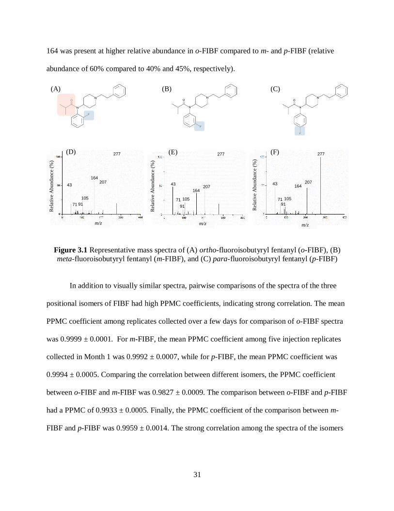
31

164 was present at higher relative abundance in o-FIBF compared to m- and p-FIBF (relative

abundance of 60% compared to 40% and 45%, respectively).

Figure 3.1 Representative mass spectra of (A) ortho-fluoroisobutyryl fentanyl (o-FIBF), (B)

meta-fluoroisobutyryl fentanyl (m-FIBF), and (C) para-fluoroisobutyryl fentanyl (p-FIBF)

In addition to visually similar spectra, pairwise comparisons of the spectra of the three

positional isomers of FIBF had high PPMC coefficients, indicating strong correlation. The mean

PPMC coefficient among replicates collected over a few days for comparison of o-FIBF spectra

was 0.9999 ± 0.0001. For m-FIBF, the mean PPMC coefficient among five injection replicates

collected in Month 1 was 0.9992 ± 0.0007, while for p-FIBF, the mean PPMC coefficient was

0.9994 ± 0.0005. Comparing the correlation between different isomers, the PPMC coefficient

between o-FIBF and m-FIBF was 0.9827 ± 0.0009. The comparison between o-FIBF and p-FIBF

had a PPMC of 0.9933 ± 0.0005. Finally, the PPMC coefficient of the comparison between m-

FIBF and p-FIBF was 0.9959 ± 0.0014. The strong correlation among the spectra of the isomers

(A) (B) (C)

277

207164

105

43

71 91

277

207164

105

43

71

91

277

207164

105

43

7191

m/z m/z m/z

Rela

tive A

bun

dance (

%)

Rela

tiv

e A

bu

nd

an

ce (

%)

Rela

tiv

e A

bu

nd

an

ce (

%)

(D) (E) (F)

32

demonstrates the level of spectral similarity, which makes it difficult to differentiate one isomer

from another when relying solely on visual inspection of spectra.

The spectral data were also searched against the National Institute of Standards and

Technology/Environmental Protection Agency/National Institutes of Health (NIST/EPA/NIH)

Mass Spectral Library, using the probability-based matching (PBM) algorithm in the Agilent

software. For the FIBF isomers, for five replicates of o-FIBF, the top hit was always p-FBF,

which is a different structural isomer that will be described in the next section. The match quality

was 81 for four of the five replicates and 90 for one. The second hit for the five replicates of o-

FIBF was o-FBF, again a structural isomer, with a match quality of 70. For the five replicates of

m-FIBF, four resulted in top hits of p-FBF and one had a top hit of o-FBF with a match quality

ranging from 62 to 83. Finally, for the five replicates of p-FIBF, four of the top hits were labeled

FIBF without any positional isomer information and one of the top hits was p-FBF. The match

qualities were either 90 or 93. Although there is no confirmation, it is believed that the mass

spectra of o-FIBF and m-FIBF reference standards are not included in the library and FIBF is

considered to be the para isomer. However, it is interesting that the top hits for both o-FIBF and

m-FIBF were isomers of FBF instead of FIBF.

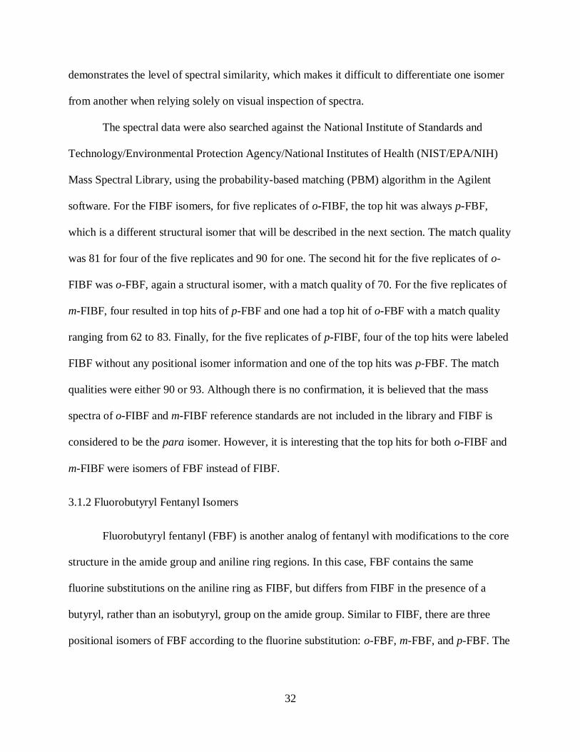
3.1.2 Fluorobutyryl Fentanyl Isomers

Fluorobutyryl fentanyl (FBF) is another analog of fentanyl with modifications to the core

structure in the amide group and aniline ring regions. In this case, FBF contains the same

fluorine substitutions on the aniline ring as FIBF, but differs from FIBF in the presence of a

butyryl, rather than an isobutyryl, group on the amide group. Similar to FIBF, there are three

positional isomers of FBF according to the fluorine substitution: o-FBF, m-FBF, and p-FBF. The

33

structures of o-, m-, and p-FBF are shown in Figure 3.2 A-C, highlighting the butyryl

substitution on the amide group and the fluorine substitutions around the aniline ring.

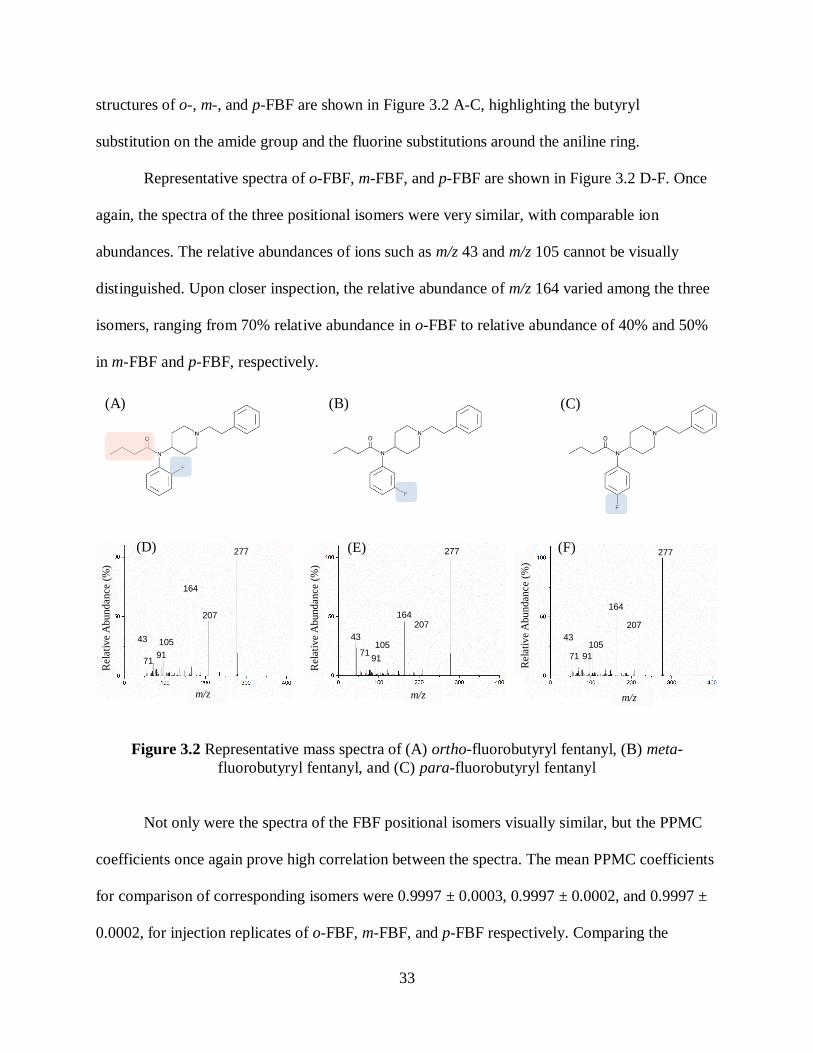
Representative spectra of o-FBF, m-FBF, and p-FBF are shown in Figure 3.2 D-F. Once

again, the spectra of the three positional isomers were very similar, with comparable ion

abundances. The relative abundances of ions such as m/z 43 and m/z 105 cannot be visually

distinguished. Upon closer inspection, the relative abundance of m/z 164 varied among the three

isomers, ranging from 70% relative abundance in o-FBF to relative abundance of 40% and 50%

in m-FBF and p-FBF, respectively.

Figure 3.2 Representative mass spectra of (A) ortho-fluorobutyryl fentanyl, (B) meta-

fluorobutyryl fentanyl, and (C) para-fluorobutyryl fentanyl

Not only were the spectra of the FBF positional isomers visually similar, but the PPMC

coefficients once again prove high correlation between the spectra. The mean PPMC coefficients

for comparison of corresponding isomers were 0.9997 ± 0.0003, 0.9997 ± 0.0002, and 0.9997 ±

0.0002, for injection replicates of o-FBF, m-FBF, and p-FBF respectively. Comparing the

(A) (B) (C)

207

164

10543

7191

207164

10543

7191

277

207

164

10543

71 91

m/z m/z m/z

Rela

tiv

e A

bu

nd

an

ce (

%)

Rela

tiv

e A

bu

nd

an

ce (

%)

Rela

tiv

e A

bu

nd

an

ce (

%)

(D) (E) (F)277 277

34

correlation between different isomers collected in Month 1, the PPMC coefficient between o-

FBF and m-FBF was 0.9849 ± 0.0012. The comparison between o-FBF and p-FBF had a PPMC

of 0.9924 ± 0.0009. And finally, the PPMC coefficient of the comparison between m-FBF and p-

FBF was 0.9981 ± 0.0005. While all of the PPMC coefficients demonstrate strong correlation, it

is important to note the high similarity of the spectra from different isomers.

Spectra of the FBF isomers were also compared to the NIST/EPA/NIH Mass Spectral

Library using the PBM algorithm. The correct isomer was the top hit for the five o-FBF

replicates, with match qualities of either 93 or 95. For the five replicates of m-FBF, four of the

top hits were p-FBF and one of the top hits was o-FBF, all with a match quality of 90. Finally,

for the five replicates of p-FBF, the top hit was always correct with a match quality ranging from

87 to 93. It should be noted in the case of the FBF isomers that, although not confirmed, it is

believed that the mass spectrum of m-FBF reference is not included in the library and is believed

to be the cause of the incorrect hits for m-FBF.

When visually comparing representative spectra of the FIBF isomers and the FBF

isomers (Figures 3.1 and 3.2 D-F), small differences were observed between the relative

abundances of m/z 43, 164, and 207. However, the six spectra are still very visually similar as all

six compounds are isomers of each other. The PPMC coefficients show strong correlation among

the isomers, with mean coefficients ranging from 0.9466 to 0.9882 (Appendix Table A3.1).

3.2 Intra-Month Comparisons of FIBF and FBF Spectra to FIBF Reference Spectra

While comparisons were performed for all pairwise combinations of the six isomers, this

chapter focuses on comparison of FIBF and FBF spectra to the FIBF reference spectra. Initially,

spectra of isomers collected each month were compared to the corresponding FIBF reference

spectra collected the same month.

35

3.2.1 Month 1 FIBF and FBF Spectra Compared to the Month 1 FIBF Reference Spectra

The FIBF and FBF comparison spectra collected in Month 1 were compared to the

corresponding Month 1 FIBF reference spectra. In Month 1, two collections of FIBF comparison

spectra samples were analyzed – Month 1A and Month 1B – to be compared to the same Month

1 reference spectra. These comparisons were used to evaluate the effect of variation in the

spectral intensities on the ability to properly associate and discriminate the spectra. The two

collections were only made for the FIBF isomers in Month 1.

Corresponding spectra of o-FIBF were statistically associated at the 99.9% confidence

level (Table 3.1). For these comparisons, spectrum A and spectrum B (from Month 1A and 1B,

respectively) were correctly associated to the o-FIBF reference spectra with a minimum random-

match probability (Pmin) of 4.749x10-55 and a maximum random-match probability (Pmax) of

4.157x10-24 calculated across the scan range m/z 40-400. Similarly, corresponding spectra of m-

FIBF were statistically associated at the 99.9% confidence level (Table 3.1). Both m-FIBF

comparison spectrum A and B were associated to the corresponding m-FIBF reference spectra at

the 99.9% confidence level with Pmin = 2.474x10-52 and Pmax = 1.185x10-24. These low random-

match probabilities demonstrate how unlikely it was that the mass spectral patterns occurred by

random chance alone.

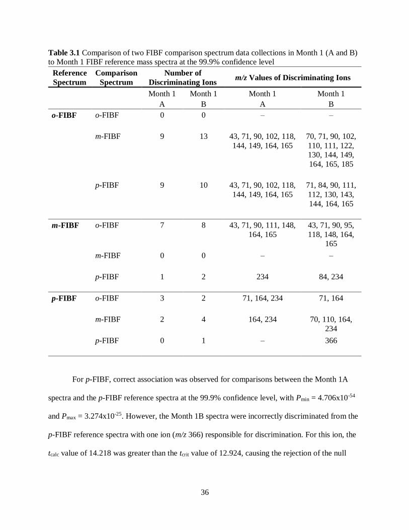
36

Table 3.1 Comparison of two FIBF comparison spectrum data collections in Month 1 (A and B)

to Month 1 FIBF reference mass spectra at the 99.9% confidence level

Reference

Spectrum

Comparison

Spectrum

Number of

Discriminating Ions m/z Values of Discriminating Ions

Month 1

A

Month 1

B

Month 1

A

Month 1

B

o-FIBF o-FIBF

0 0 – –

m-FIBF 9 13 43, 71, 90, 102, 118,

144, 149, 164, 165

70, 71, 90, 102,

110, 111, 122,

130, 144, 149,

164, 165, 185

p-FIBF 9 10 43, 71, 90, 102, 118,

144, 149, 164, 165

71, 84, 90, 111,

112, 130, 143,

144, 164, 165

m-FIBF o-FIBF 7 8 43, 71, 90, 111, 148,

164, 165

43, 71, 90, 95,

118, 148, 164,

165

m-FIBF

0 0 – –

p-FIBF 1 2 234 84, 234

p-FIBF o-FIBF

3 2 71, 164, 234 71, 164

m-FIBF

2 4 164, 234 70, 110, 164,

234

p-FIBF

0 1 – 366

For p-FIBF, correct association was observed for comparisons between the Month 1A

spectra and the p-FIBF reference spectra at the 99.9% confidence level, with Pmin = 4.706x10-54

and Pmax = 3.274x10-25. However, the Month 1B spectra were incorrectly discriminated from the

p-FIBF reference spectra with one ion (m/z 366) responsible for discrimination. For this ion, the

tcalc value of 14.218 was greater than the tcrit value of 12.924, causing the rejection of the null

37

hypothesis. The chemical relevance of m/z 366 is not known, but the ion does not appear as a

common discriminating ion in other comparisons.

In terms of discrimination, the Month 1 FIBF comparison spectra were correctly

discriminated from the other FIBF reference spectra in all cases (Table 3.1). There was a similar

number of discriminating ions between the spectrum A and spectrum B comparisons in Month 1,

however the identities of those ions varied between each collection.

The m- and p-FIBF comparison spectra were discriminated from the o-FIBF reference

spectra at the 99.9% confidence level (Table 3.1). The m-FIBF to o-FIBF comparison resulted in

9 discriminating ions for the Month 1A collection and 13 discriminating ions for the Month 1B

collection. Common discriminating ions between the spectra of m- and o-FIBF for both

collections included m/z 71, 90, 102, 144, 149, 164, and 165. The p-FIBF to o-FIBF reference

spectra comparison resulted in 9 discriminating ions for the Month 1A spectrum and 10

discriminating ions for the Month 1B spectrum. The month 1A and 1B comparisons of p-FIBF to

o-FIBF resulted in common ions between both collections such as m/z 71, 90, 144, 164, and 165.

Discrimination of the o- and p-FIBF comparison spectra from the m-FIBF reference

spectra was also possible at the 99.9% confidence level (Table 3.1). For o-FIBF compared to the

m-FIBF reference, 7 and 8 ions were responsible for discrimination in the Month 1A spectrum

and Month 1B spectrum, respectively. Common discriminating ions between o- and m-FIBF for

both collections included m/z 43, 71, 90, 148, 164, and 165. For p-FIBF comparison spectra and

the m-FIBF reference, discrimination was also observed at the 99.9% confidence level, with 1 to

2 discriminating ions observed (Table 3.1). For Month 1A, the discriminating ion was m/z 234,

whereas for Month 1B, m/z 234 and m/z 84 were discriminating ions.

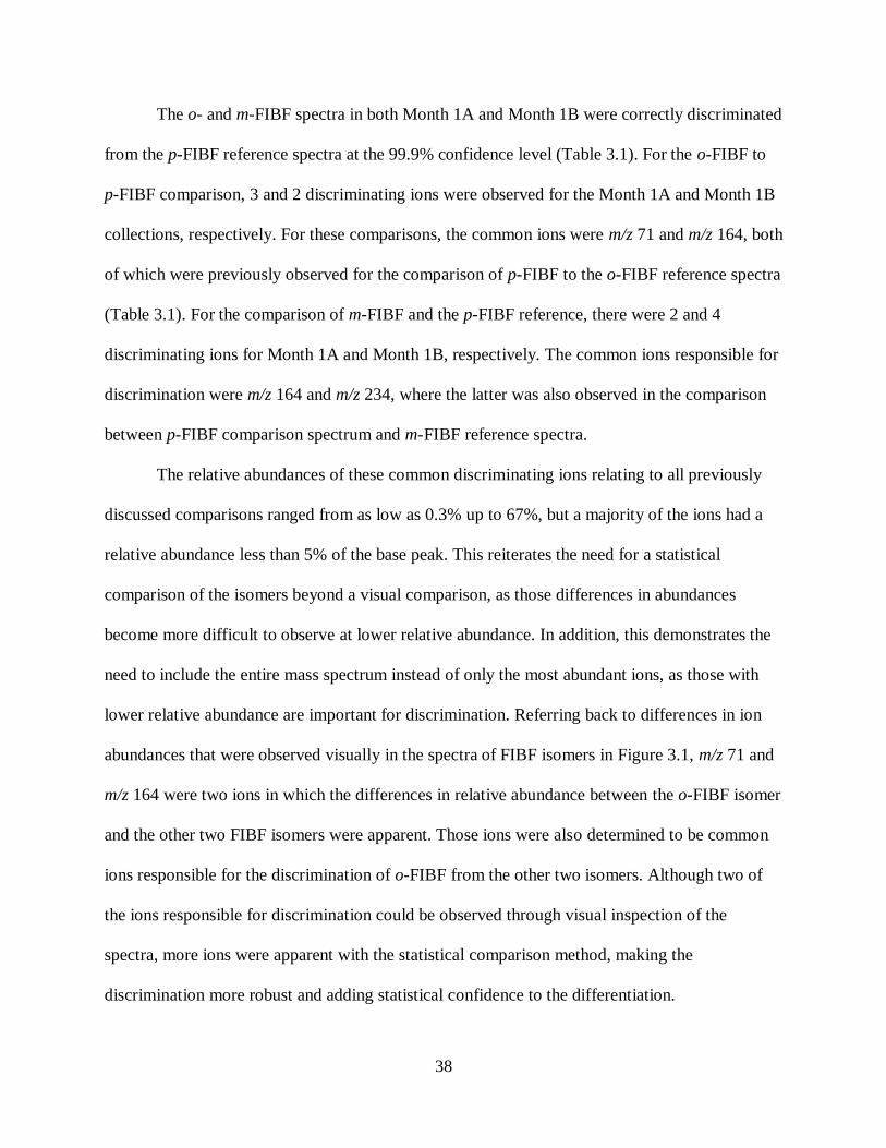
38

The o- and m-FIBF spectra in both Month 1A and Month 1B were correctly discriminated

from the p-FIBF reference spectra at the 99.9% confidence level (Table 3.1). For the o-FIBF to

p-FIBF comparison, 3 and 2 discriminating ions were observed for the Month 1A and Month 1B

collections, respectively. For these comparisons, the common ions were m/z 71 and m/z 164, both

of which were previously observed for the comparison of p-FIBF to the o-FIBF reference spectra

(Table 3.1). For the comparison of m-FIBF and the p-FIBF reference, there were 2 and 4

discriminating ions for Month 1A and Month 1B, respectively. The common ions responsible for

discrimination were m/z 164 and m/z 234, where the latter was also observed in the comparison

between p-FIBF comparison spectrum and m-FIBF reference spectra.

The relative abundances of these common discriminating ions relating to all previously

discussed comparisons ranged from as low as 0.3% up to 67%, but a majority of the ions had a

relative abundance less than 5% of the base peak. This reiterates the need for a statistical

comparison of the isomers beyond a visual comparison, as those differences in abundances

become more difficult to observe at lower relative abundance. In addition, this demonstrates the

need to include the entire mass spectrum instead of only the most abundant ions, as those with

lower relative abundance are important for discrimination. Referring back to differences in ion

abundances that were observed visually in the spectra of FIBF isomers in Figure 3.1, m/z 71 and

m/z 164 were two ions in which the differences in relative abundance between the o-FIBF isomer

and the other two FIBF isomers were apparent. Those ions were also determined to be common

ions responsible for the discrimination of o-FIBF from the other two isomers. Although two of

the ions responsible for discrimination could be observed through visual inspection of the

spectra, more ions were apparent with the statistical comparison method, making the

discrimination more robust and adding statistical confidence to the differentiation.

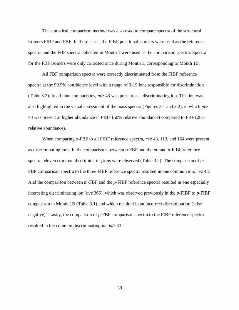
39

The statistical comparison method was also used to compare spectra of the structural

isomers FIBF and FBF. In these cases, the FIBF positional isomers were used as the reference

spectra and the FBF spectra collected in Month 1 were used as the comparison spectra. Spectra

for the FBF isomers were only collected once during Month 1, corresponding to Month 1B.

All FBF comparison spectra were correctly discriminated from the FIBF reference

spectra at the 99.9% confidence level with a range of 3-19 ions responsible for discrimination

(Table 3.2). In all nine comparisons, m/z 43 was present as a discriminating ion. This ion was

also highlighted in the visual assessment of the mass spectra (Figures 3.1 and 3.2), in which m/z

43 was present at higher abundance in FIBF (50% relative abundance) compared to FBF (28%

relative abundance).

When comparing o-FBF to all FIBF reference spectra, m/z 43, 113, and 164 were present

as discriminating ions. In the comparisons between o-FBF and the m- and p-FIBF reference

spectra, eleven common discriminating ions were observed (Table 3.2). The comparison of m-

FBF comparison spectra to the three FIBF reference spectra resulted in one common ion, m/z 43.

And the comparison between m-FBF and the p-FIBF reference spectra resulted in one especially

interesting discriminating ion (m/z 366), which was observed previously in the p-FIBF to p-FIBF

comparison in Month 1B (Table 3.1) and which resulted in an incorrect discrimination (false

negative). Lastly, the comparison of p-FBF comparison spectra to the FIBF reference spectra

resulted in the common discriminating ion m/z 43.

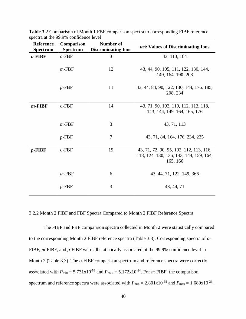
40


spectra at the 99.9% confidence level

Reference

Spectrum

Comparison

Spectrum

Number of


o-FIBF o-FBF

3 43, 113, 164

m-FBF

12 43, 44, 90, 105, 111, 122, 130, 144,

149, 164, 190, 208

p-FBF 11 43, 44, 84, 90, 122, 130, 144, 176, 185,

208, 234

m-FIBF o-FBF

14 43, 71, 90, 102, 110, 112, 113, 118,

143, 144, 149, 164, 165, 176

m-FBF

3 43, 71, 113

p-FBF

7 43, 71, 84, 164, 176, 234, 235

p-FIBF o-FBF

19 43, 71, 72, 90, 95, 102, 112, 113, 116,

118, 124, 130, 136, 143, 144, 159, 164,

165, 166

m-FBF

6 43, 44, 71, 122, 149, 366

p-FBF

3 43, 44, 71

3.2.2 Month 2 FIBF and FBF Spectra Compared to Month 2 FIBF Reference Spectra

The FIBF and FBF comparison spectra collected in Month 2 were statistically compared

to the corresponding Month 2 FIBF reference spectra (Table 3.3). Corresponding spectra of o-

FIBF, m-FIBF, and p-FIBF were all statistically associated at the 99.9% confidence level in

Month 2 (Table 3.3). The o-FIBF comparison spectrum and reference spectra were correctly

associated with Pmin = 5.731x10-56 and Pmax = 5.172x10-24. For m-FIBF, the comparison

spectrum and reference spectra were associated with Pmin = 2.801x10-55 and Pmax = 1.680x10-23.

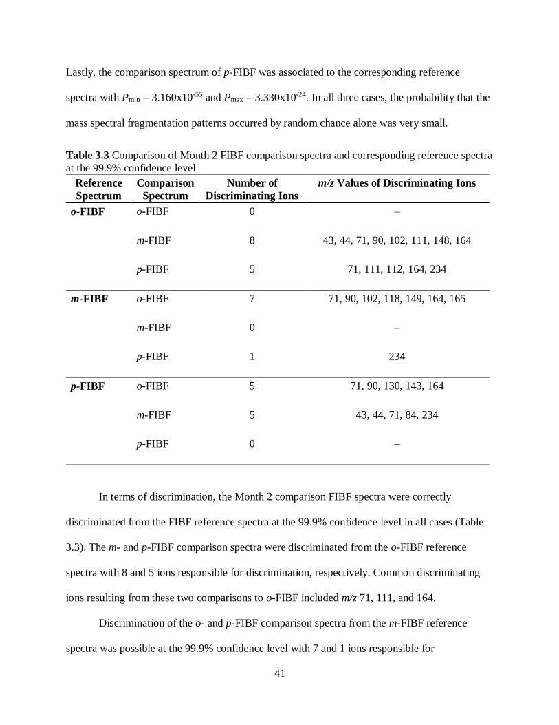
41

Lastly, the comparison spectrum of p-FIBF was associated to the corresponding reference

spectra with Pmin = 3.160x10-55 and Pmax = 3.330x10-24. In all three cases, the probability that the

mass spectral fragmentation patterns occurred by random chance alone was very small.


at the 99.9% confidence level

Reference

Spectrum

Comparison

Spectrum

Number of

Discriminating Ions

m/z Values of Discriminating Ions

o-FIBF o-FIBF

0 –

m-FIBF

8 43, 44, 71, 90, 102, 111, 148, 164

p-FIBF 5 71, 111, 112, 164, 234

m-FIBF o-FIBF

7 71, 90, 102, 118, 149, 164, 165

m-FIBF

0 –

p-FIBF

1 234

p-FIBF o-FIBF

5 71, 90, 130, 143, 164

m-FIBF

5 43, 44, 71, 84, 234

p-FIBF

0 –

In terms of discrimination, the Month 2 comparison FIBF spectra were correctly

discriminated from the FIBF reference spectra at the 99.9% confidence level in all cases (Table

3.3). The m- and p-FIBF comparison spectra were discriminated from the o-FIBF reference

spectra with 8 and 5 ions responsible for discrimination, respectively. Common discriminating

ions resulting from these two comparisons to o-FIBF included m/z 71, 111, and 164.

Discrimination of the o- and p-FIBF comparison spectra from the m-FIBF reference

spectra was possible at the 99.9% confidence level with 7 and 1 ions responsible for

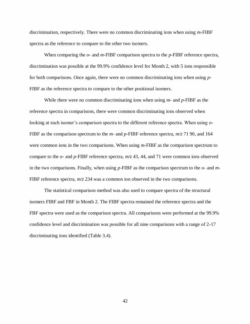
42

discrimination, respectively. There were no common discriminating ions when using m-FIBF

spectra as the reference to compare to the other two isomers.

When comparing the o- and m-FIBF comparison spectra to the p-FIBF reference spectra,

discrimination was possible at the 99.9% confidence level for Month 2, with 5 ions responsible

for both comparisons. Once again, there were no common discriminating ions when using p-

FIBF as the reference spectra to compare to the other positional isomers.

While there were no common discriminating ions when using m- and p-FIBF as the

reference spectra in comparisons, there were common discriminating ions observed when

looking at each isomer’s comparison spectra to the different reference spectra. When using o-

FIBF as the comparison spectrum to the m- and p-FIBF reference spectra, m/z 71 90, and 164

were common ions in the two comparisons. When using m-FIBF as the comparison spectrum to

compare to the o- and p-FIBF reference spectra, m/z 43, 44, and 71 were common ions observed

in the two comparisons. Finally, when using p-FIBF as the comparison spectrum to the o- and m-

FIBF reference spectra, m/z 234 was a common ion observed in the two comparisons.

The statistical comparison method was also used to compare spectra of the structural

isomers FIBF and FBF in Month 2. The FIBF spectra remained the reference spectra and the

FBF spectra were used as the comparison spectra. All comparisons were performed at the 99.9%

confidence level and discrimination was possible for all nine comparisons with a range of 2-17

discriminating ions identified (Table 3.4).

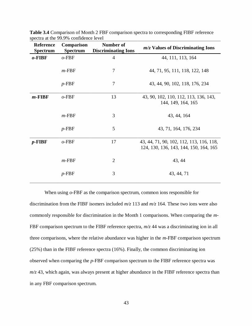
43



Reference

Spectrum

Comparison

Spectrum

Number of


o-FIBF o-FBF

4 44, 111, 113, 164

m-FBF

7 44, 71, 95, 111, 118, 122, 148

p-FBF 7 43, 44, 90, 102, 118, 176, 234

m-FIBF o-FBF

13 43, 90, 102, 110, 112, 113, 136, 143,

144, 149, 164, 165

m-FBF

3 43, 44, 164

p-FBF

5 43, 71, 164, 176, 234

p-FIBF o-FBF

17 43, 44, 71, 90, 102, 112, 113, 116, 118,

124, 130, 136, 143, 144, 150, 164, 165

m-FBF

2 43, 44

p-FBF

3 43, 44, 71

When using o-FBF as the comparison spectrum, common ions responsible for

discrimination from the FIBF isomers included m/z 113 and m/z 164. These two ions were also

commonly responsible for discrimination in the Month 1 comparisons. When comparing the m-

FBF comparison spectrum to the FIBF reference spectra, m/z 44 was a discriminating ion in all

three comparisons, where the relative abundance was higher in the m-FBF comparison spectrum

(25%) than in the FIBF reference spectra (16%). Finally, the common discriminating ion

observed when comparing the p-FBF comparison spectrum to the FIBF reference spectra was

m/z 43, which again, was always present at higher abundance in the FIBF reference spectra than

in any FBF comparison spectrum.

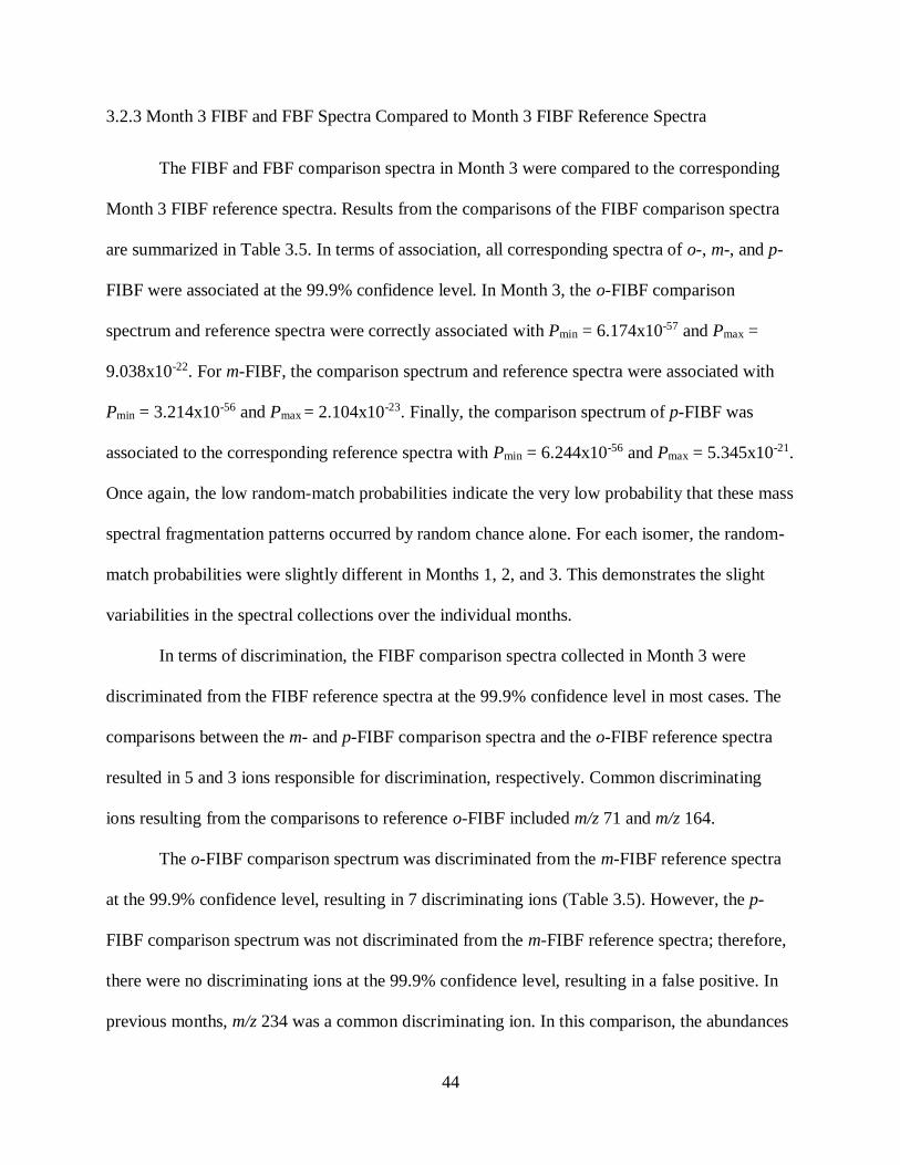
44

3.2.3 Month 3 FIBF and FBF Spectra Compared to Month 3 FIBF Reference Spectra

The FIBF and FBF comparison spectra in Month 3 were compared to the corresponding

Month 3 FIBF reference spectra. Results from the comparisons of the FIBF comparison spectra

are summarized in Table 3.5. In terms of association, all corresponding spectra of o-, m-, and p-

FIBF were associated at the 99.9% confidence level. In Month 3, the o-FIBF comparison

spectrum and reference spectra were correctly associated with Pmin = 6.174x10-57 and Pmax =

9.038x10-22. For m-FIBF, the comparison spectrum and reference spectra were associated with

Pmin = 3.214x10-56 and Pmax = 2.104x10-23. Finally, the comparison spectrum of p-FIBF was

associated to the corresponding reference spectra with Pmin = 6.244x10-56 and Pmax = 5.345x10-21.

Once again, the low random-match probabilities indicate the very low probability that these mass

spectral fragmentation patterns occurred by random chance alone. For each isomer, the random-

match probabilities were slightly different in Months 1, 2, and 3. This demonstrates the slight

variabilities in the spectral collections over the individual months.

In terms of discrimination, the FIBF comparison spectra collected in Month 3 were

discriminated from the FIBF reference spectra at the 99.9% confidence level in most cases. The

comparisons between the m- and p-FIBF comparison spectra and the o-FIBF reference spectra

resulted in 5 and 3 ions responsible for discrimination, respectively. Common discriminating

ions resulting from the comparisons to reference o-FIBF included m/z 71 and m/z 164.

The o-FIBF comparison spectrum was discriminated from the m-FIBF reference spectra

at the 99.9% confidence level, resulting in 7 discriminating ions (Table 3.5). However, the p-

FIBF comparison spectrum was not discriminated from the m-FIBF reference spectra; therefore,

there were no discriminating ions at the 99.9% confidence level, resulting in a false positive. In

previous months, m/z 234 was a common discriminating ion. In this comparison, the abundances

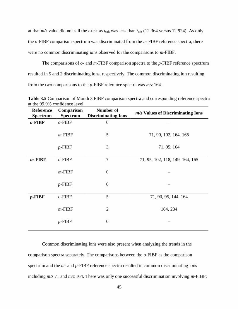
45

at that m/z value did not fail the t-test as tcalc was less than tcrit (12.364 versus 12.924). As only

the o-FIBF comparison spectrum was discriminated from the m-FIBF reference spectra, there

were no common discriminating ions observed for the comparisons to m-FIBF.

The comparisons of o- and m-FIBF comparison spectra to the p-FIBF reference spectrum

resulted in 5 and 2 discriminating ions, respectively. The common discriminating ion resulting

from the two comparisons to the p-FIBF reference spectra was m/z 164.


at the 99.9% confidence level

Reference

Spectrum

Comparison

Spectrum

Number of


o-FIBF o-FIBF

0 –

m-FIBF

5 71, 90, 102, 164, 165

p-FIBF 3 71, 95, 164

m-FIBF o-FIBF

7 71, 95, 102, 118, 149, 164, 165

m-FIBF

0 –

p-FIBF

0 –

p-FIBF o-FIBF

5 71, 90, 95, 144, 164

m-FIBF

2 164, 234

p-FIBF

0 –

Common discriminating ions were also present when analyzing the trends in the

comparison spectra separately. The comparisons between the o-FIBF as the comparison

spectrum and the m- and p-FIBF reference spectra resulted in common discriminating ions

including m/z 71 and m/z 164. There was only one successful discrimination involving m-FIBF;

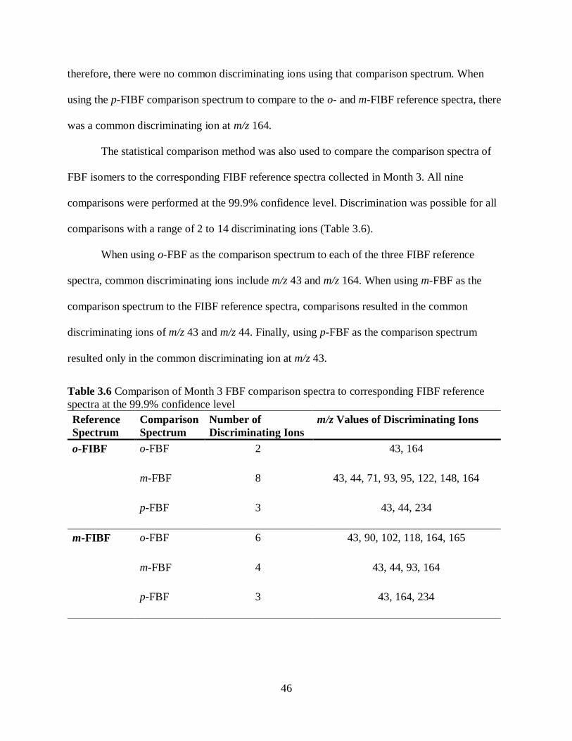
46

therefore, there were no common discriminating ions using that comparison spectrum. When

using the p-FIBF comparison spectrum to compare to the o- and m-FIBF reference spectra, there

was a common discriminating ion at m/z 164.

The statistical comparison method was also used to compare the comparison spectra of

FBF isomers to the corresponding FIBF reference spectra collected in Month 3. All nine

comparisons were performed at the 99.9% confidence level. Discrimination was possible for all

comparisons with a range of 2 to 14 discriminating ions (Table 3.6).

When using o-FBF as the comparison spectrum to each of the three FIBF reference

spectra, common discriminating ions include m/z 43 and m/z 164. When using m-FBF as the

comparison spectrum to the FIBF reference spectra, comparisons resulted in the common

discriminating ions of m/z 43 and m/z 44. Finally, using p-FBF as the comparison spectrum

resulted only in the common discriminating ion at m/z 43.



Reference

Spectrum

Comparison

Spectrum

Number of

Discriminating Ions


o-FIBF o-FBF

2 43, 164

m-FBF

8 43, 44, 71, 93, 95, 122, 148, 164

p-FBF 3 43, 44, 234

m-FIBF o-FBF

6 43, 90, 102, 118, 164, 165

m-FBF

4 43, 44, 93, 164

p-FBF

3 43, 164, 234

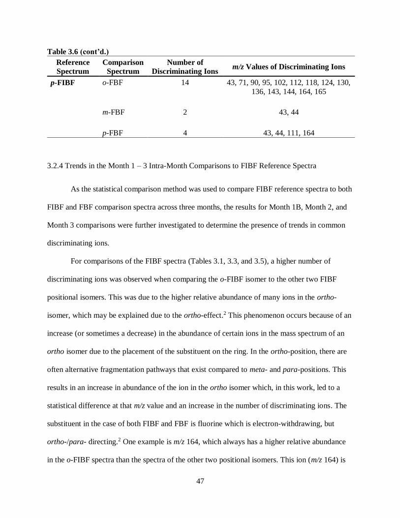
47

Table 3.6 (cont’d.)

Reference

Spectrum

Comparison

Spectrum

Number of


p-FIBF o-FBF

14 43, 71, 90, 95, 102, 112, 118, 124, 130,

136, 143, 144, 164, 165

m-FBF

2 43, 44

p-FBF 4 43, 44, 111, 164

3.2.4 Trends in the Month 1 – 3 Intra-Month Comparisons to FIBF Reference Spectra

As the statistical comparison method was used to compare FIBF reference spectra to both

FIBF and FBF comparison spectra across three months, the results for Month 1B, Month 2, and

Month 3 comparisons were further investigated to determine the presence of trends in common

discriminating ions.

For comparisons of the FIBF spectra (Tables 3.1, 3.3, and 3.5), a higher number of

discriminating ions was observed when comparing the o-FIBF isomer to the other two FIBF

positional isomers. This was due to the higher relative abundance of many ions in the ortho-

isomer, which may be explained due to the ortho-effect.2 This phenomenon occurs because of an

increase (or sometimes a decrease) in the abundance of certain ions in the mass spectrum of an

ortho isomer due to the placement of the substituent on the ring. In the ortho-position, there are

often alternative fragmentation pathways that exist compared to meta- and para-positions. This

results in an increase in abundance of the ion in the ortho isomer which, in this work, led to a

statistical difference at that m/z value and an increase in the number of discriminating ions. The

substituent in the case of both FIBF and FBF is fluorine which is electron-withdrawing, but

ortho-/para- directing.2 One example is m/z 164, which always has a higher relative abundance

in the o-FIBF spectra than the spectra of the other two positional isomers. This ion (m/z 164) is

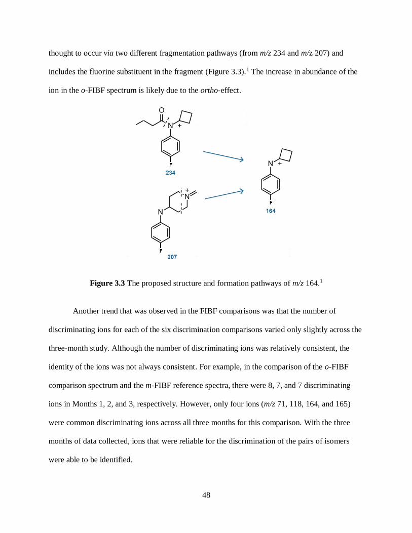
48

thought to occur via two different fragmentation pathways (from m/z 234 and m/z 207) and

includes the fluorine substituent in the fragment (Figure 3.3).1 The increase in abundance of the

ion in the o-FIBF spectrum is likely due to the ortho-effect.

Figure 3.3 The proposed structure and formation pathways of m/z 164.1

Another trend that was observed in the FIBF comparisons was that the number of

discriminating ions for each of the six discrimination comparisons varied only slightly across the

three-month study. Although the number of discriminating ions was relatively consistent, the

identity of the ions was not always consistent. For example, in the comparison of the o-FIBF

comparison spectrum and the m-FIBF reference spectra, there were 8, 7, and 7 discriminating

ions in Months 1, 2, and 3, respectively. However, only four ions (m/z 71, 118, 164, and 165)

were common discriminating ions across all three months for this comparison. With the three

months of data collected, ions that were reliable for the discrimination of the pairs of isomers

were able to be identified.

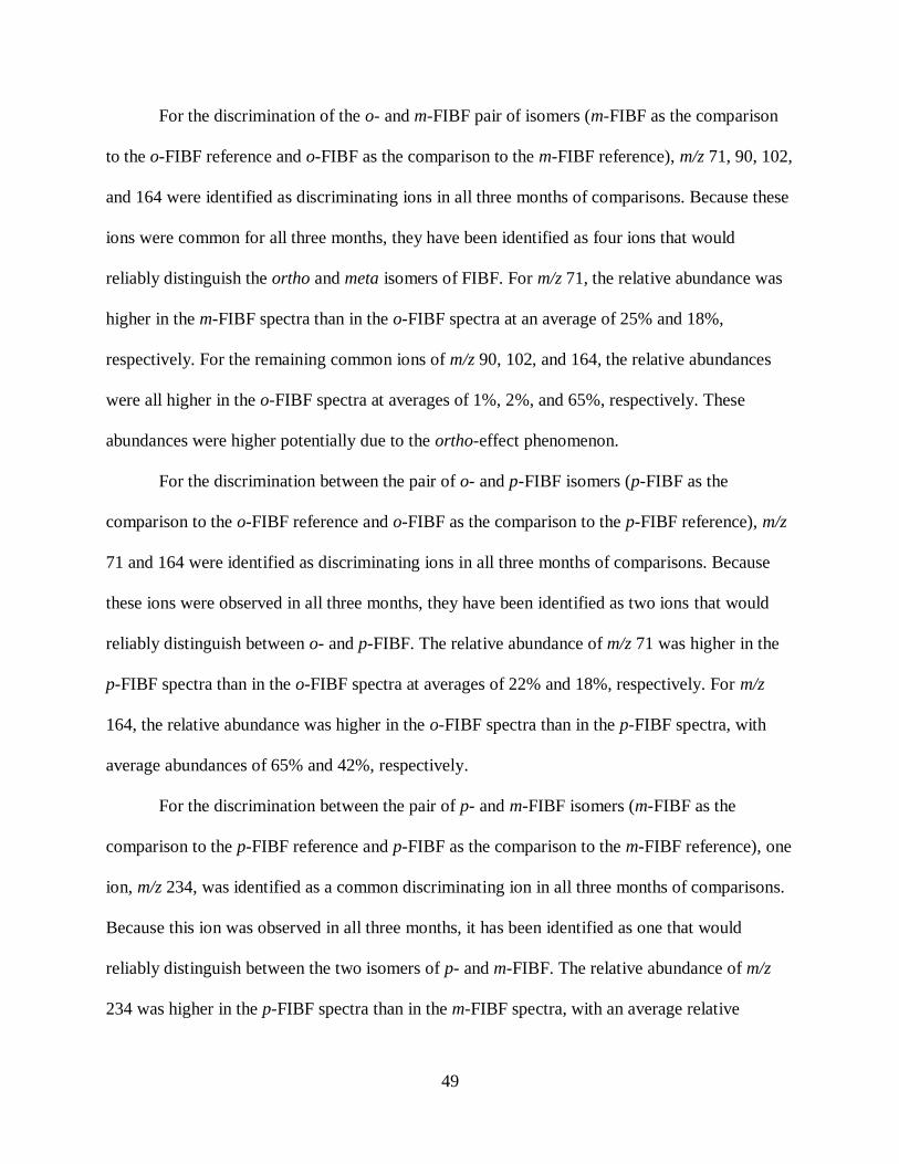
49

For the discrimination of the o- and m-FIBF pair of isomers (m-FIBF as the comparison

to the o-FIBF reference and o-FIBF as the comparison to the m-FIBF reference), m/z 71, 90, 102,

and 164 were identified as discriminating ions in all three months of comparisons. Because these

ions were common for all three months, they have been identified as four ions that would

reliably distinguish the ortho and meta isomers of FIBF. For m/z 71, the relative abundance was

higher in the m-FIBF spectra than in the o-FIBF spectra at an average of 25% and 18%,

respectively. For the remaining common ions of m/z 90, 102, and 164, the relative abundances

were all higher in the o-FIBF spectra at averages of 1%, 2%, and 65%, respectively. These

abundances were higher potentially due to the ortho-effect phenomenon.

For the discrimination between the pair of o- and p-FIBF isomers (p-FIBF as the

comparison to the o-FIBF reference and o-FIBF as the comparison to the p-FIBF reference), m/z

71 and 164 were identified as discriminating ions in all three months of comparisons. Because

these ions were observed in all three months, they have been identified as two ions that would

reliably distinguish between o- and p-FIBF. The relative abundance of m/z 71 was higher in the

p-FIBF spectra than in the o-FIBF spectra at averages of 22% and 18%, respectively. For m/z

164, the relative abundance was higher in the o-FIBF spectra than in the p-FIBF spectra, with

average abundances of 65% and 42%, respectively.

For the discrimination between the pair of p- and m-FIBF isomers (m-FIBF as the

comparison to the p-FIBF reference and p-FIBF as the comparison to the m-FIBF reference), one

ion, m/z 234, was identified as a common discriminating ion in all three months of comparisons.

Because this ion was observed in all three months, it has been identified as one that would

reliably distinguish between the two isomers of p- and m-FIBF. The relative abundance of m/z

234 was higher in the p-FIBF spectra than in the m-FIBF spectra, with an average relative

50

abundance of 4% and 3%, respectively. While there is only a 1% difference in abundance here,

this was a statistically significant difference that enabled the distinction of the two isomers.

For the trends in the comparisons between the FBF comparison spectra and the FIBF

reference spectra, overall, there was a higher number of discriminating ions present, as expected,

ranging from 3 – 19 ions for the comparisons (Tables 3.2, 3.4, and 3.6). Common ions that

resulted in discrimination of all of the FBF comparison spectra from the o-FIBF reference

spectra in all three months included m/z 43, 44, 111, 122, and 164. For m/z 43, 111, and 122, the

average relative abundance of the o-FIBF reference spectra was higher than the relative

abundance of each of the FBF comparison spectra. For example, the relative abundance of m/z

111 was 6% in the o-FIBF reference spectra and 4% in the FBF comparison spectra. The

abundance of m/z 122 was 8% in the o-FIBF reference spectra and 6% in the FBF comparison

spectra. For m/z 44 and m/z 164, the opposite was true. The relative abundance of m/z 44 was

lower at 21% in the o-FIBF reference spectra and higher at 35% in the FBF comparison spectra.

Common ions that resulted in discrimination of the FBF comparison spectra from the m-

FIBF reference spectra across the three months included m/z 43, 71, 164, and 234. For m/z 43

and m/z 71, the relative abundances were higher in the FIBF reference spectra with averages of

45% and 20%, respectively. However; the relative abundances of m/z 164 (68%) and m/z 234

(5%) were higher in the FBF comparison spectra.

Finally, when comparing the FBF comparison spectra to the p-FIBF reference spectra,

only m/z 43 was identified as a common discriminating ion observed in all three months.

Following the same trends as the comparisons to the other two FIBF isomers as reference

spectra, the relative abundance of m/z 43 was higher in the p-FIBF spectra than in the FBF

comparison spectra.

51

All nine discrimination comparisons between FBF and FIBF included m/z 43 as a

discriminating ion. For each of the nine comparisons, the average relative abundance of this ion

was higher for the FIBF reference spectra than the FBF comparison spectra, which has been

demonstrated repeatedly. Referring back to the spectra of FIBF and FBF isomers in Figures 3.1

and 3.2, there was a visual difference in the abundance of m/z 43 between the FIBF and FBF

spectra. Some of the common ions observed in the FBF to FIBF reference spectra comparisons

were also observed in the FIBF to FIBF comparisons (m/z 43, 71, 90, 164, and 234). However,

there were ions that were not observed during the FIBF to FIBF comparisons including low

abundance ions (below 5% of the base peak) such as m/z 102, 111, 118, 122, 124, 130, 136, 143,

and 165. The relative abundances of these ions ranged from 0.2% to 10%.

Comparisons were also made using FBF isomers as the reference spectra to the FBF and

FIBF isomers as comparison spectra. The results of these comparisons are shown in Appendix

Tables A3.2 – A3.7. The overall trends for these comparisons were similar to the trends observed

in the FIBF comparisons. However, there were some differences in the identities of the ions

responsible for discrimination in the FBF to FBF comparisons and the FIBF to FBF

comparisons.

3.4 Inter-Month Comparisons of FIBF and FBF Spectra to FIBF Reference Spectra

Because the electron multiplier response between Month 1 and Month 2 was not

statistically different, comparisons of spectra collected between these two months were

compared. Spectra collected in Month 1 were retained as the reference to which spectra of FIBF

and FBF collected in Month 2 were compared.

For comparisons of FIBF comparison spectra collected in Month 2 to the FIBF reference

spectra collected in Month 1, no association was observed, resulting in three instances of

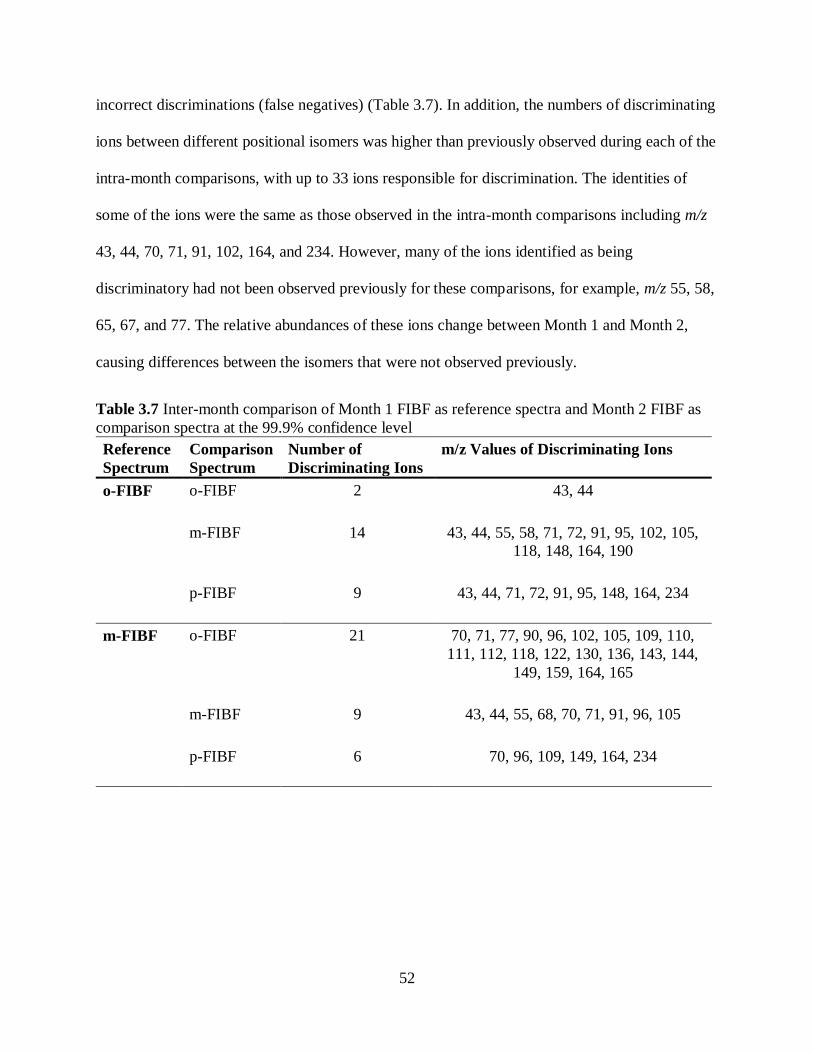
52

incorrect discriminations (false negatives) (Table 3.7). In addition, the numbers of discriminating

ions between different positional isomers was higher than previously observed during each of the

intra-month comparisons, with up to 33 ions responsible for discrimination. The identities of

some of the ions were the same as those observed in the intra-month comparisons including m/z

43, 44, 70, 71, 91, 102, 164, and 234. However, many of the ions identified as being

discriminatory had not been observed previously for these comparisons, for example, m/z 55, 58,

65, 67, and 77. The relative abundances of these ions change between Month 1 and Month 2,

causing differences between the isomers that were not observed previously.

Table 3.7 Inter-month comparison of Month 1 FIBF as reference spectra and Month 2 FIBF as

comparison spectra at the 99.9% confidence level

Reference

Spectrum

Comparison

Spectrum

Number of

Discriminating Ions


o-FIBF o-FIBF

2 43, 44

m-FIBF

14 43, 44, 55, 58, 71, 72, 91, 95, 102, 105,

118, 148, 164, 190

p-FIBF 9 43, 44, 71, 72, 91, 95, 148, 164, 234

m-FIBF o-FIBF

21 70, 71, 77, 90, 96, 102, 105, 109, 110,

111, 112, 118, 122, 130, 136, 143, 144,

149, 159, 164, 165

m-FIBF

9 43, 44, 55, 68, 70, 71, 91, 96, 105

p-FIBF

6 70, 96, 109, 149, 164, 234

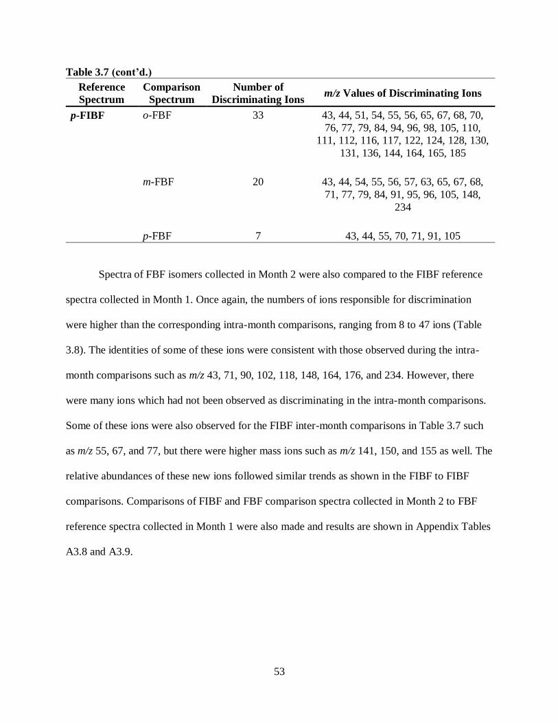
53


Reference

Spectrum

Comparison

Spectrum

Number of


p-FIBF o-FBF

33 43, 44, 51, 54, 55, 56, 65, 67, 68, 70,

76, 77, 79, 84, 94, 96, 98, 105, 110,

111, 112, 116, 117, 122, 124, 128, 130,

131, 136, 144, 164, 165, 185

m-FBF

20 43, 44, 54, 55, 56, 57, 63, 65, 67, 68,

71, 77, 79, 84, 91, 95, 96, 105, 148,

234

p-FBF 7 43, 44, 55, 70, 71, 91, 105

Spectra of FBF isomers collected in Month 2 were also compared to the FIBF reference

spectra collected in Month 1. Once again, the numbers of ions responsible for discrimination

were higher than the corresponding intra-month comparisons, ranging from 8 to 47 ions (Table

3.8). The identities of some of these ions were consistent with those observed during the intra-

month comparisons such as m/z 43, 71, 90, 102, 118, 148, 164, 176, and 234. However, there

were many ions which had not been observed as discriminating in the intra-month comparisons.

Some of these ions were also observed for the FIBF inter-month comparisons in Table 3.7 such

as m/z 55, 67, and 77, but there were higher mass ions such as m/z 141, 150, and 155 as well. The

relative abundances of these new ions followed similar trends as shown in the FIBF to FIBF

comparisons. Comparisons of FIBF and FBF comparison spectra collected in Month 2 to FBF

reference spectra collected in Month 1 were also made and results are shown in Appendix Tables

A3.8 and A3.9.

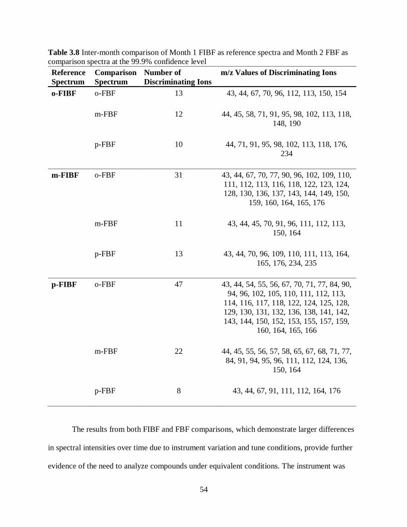
54

Table 3.8 Inter-month comparison of Month 1 FIBF as reference spectra and Month 2 FBF as


Reference

Spectrum

Comparison

Spectrum

Number of

Discriminating Ions


o-FIBF o-FBF

13 43, 44, 67, 70, 96, 112, 113, 150, 154

m-FBF

12 44, 45, 58, 71, 91, 95, 98, 102, 113, 118,

148, 190

p-FBF 10 44, 71, 91, 95, 98, 102, 113, 118, 176,

234

m-FIBF o-FBF

31 43, 44, 67, 70, 77, 90, 96, 102, 109, 110,

111, 112, 113, 116, 118, 122, 123, 124,

128, 130, 136, 137, 143, 144, 149, 150,

159, 160, 164, 165, 176

m-FBF

11 43, 44, 45, 70, 91, 96, 111, 112, 113,

150, 164

p-FBF 13 43, 44, 70, 96, 109, 110, 111, 113, 164,

165, 176, 234, 235

p-FIBF o-FBF

47 43, 44, 54, 55, 56, 67, 70, 71, 77, 84, 90,

94, 96, 102, 105, 110, 111, 112, 113,

114, 116, 117, 118, 122, 124, 125, 128,

129, 130, 131, 132, 136, 138, 141, 142,

143, 144, 150, 152, 153, 155, 157, 159,

160, 164, 165, 166

m-FBF

22 44, 45, 55, 56, 57, 58, 65, 67, 68, 71, 77,

84, 91, 94, 95, 96, 111, 112, 124, 136,

150, 164

p-FBF

8 43, 44, 67, 91, 111, 112, 164, 176

The results from both FIBF and FBF comparisons, which demonstrate larger differences

in spectral intensities over time due to instrument variation and tune conditions, provide further

evidence of the need to analyze compounds under equivalent conditions. The instrument was

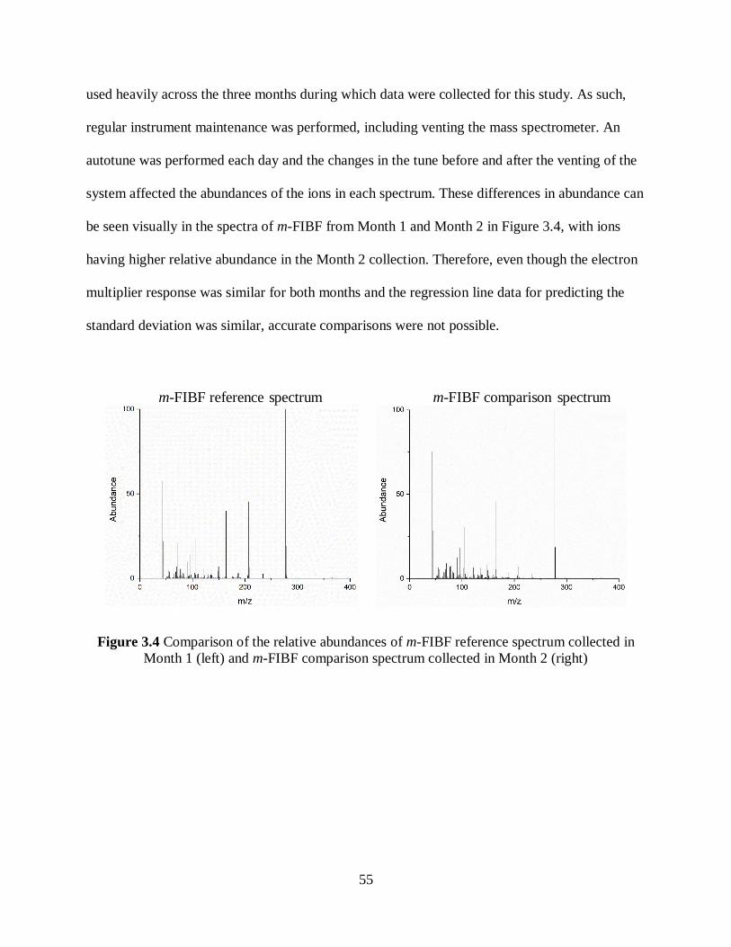
55

used heavily across the three months during which data were collected for this study. As such,

regular instrument maintenance was performed, including venting the mass spectrometer. An

autotune was performed each day and the changes in the tune before and after the venting of the

system affected the abundances of the ions in each spectrum. These differences in abundance can

be seen visually in the spectra of m-FIBF from Month 1 and Month 2 in Figure 3.4, with ions

having higher relative abundance in the Month 2 collection. Therefore, even though the electron

multiplier response was similar for both months and the regression line data for predicting the

standard deviation was similar, accurate comparisons were not possible.

Figure 3.4 Comparison of the relative abundances of m-FIBF reference spectrum collected in

Month 1 (left) and m-FIBF comparison spectrum collected in Month 2 (right)

m-FIBF reference spectrum m-FIBF comparison spectrum

56

3.5 Summary

The mass spectra of the positional isomers of FIBF and FBF were highly similar and

distinction of the isomers was not possible based on visual assessment alone. However, statistical

comparison of the spectra resulted in association and discrimination at the 99.9% confidence

level according to the specific isomer.

Intra-month comparisons of the FIBF isomers across a three-month period allowed for

the determination of common ions responsible for discrimination between each of the isomers.

Comparisons in Months 1 – 3 were also made between FBF comparison spectra and FIBF

reference spectra. This allowed for the determination of common discriminating ions between

the two sets of isomers, as well as a demonstration of the the ability of the method to

differentiate between the sets. The comparisons also showed evidence of the ortho-effect, with a

greater number of discriminating ions present when either o-FIBF or o-FBF was compared to the

other isomers.

Finally, results from the inter-month comparison between the Month 2 FIBF and FBF

comparison spectra and the Month 1 FIBF reference spectra were discussed. In this case,

association was not observed and the number of discriminating ions between the six isomers was

higher than previously observed in the intra-month comparisons. These results highlighted the

importance of analyzing the compounds to be used as the comparison spectra and the reference

spectra under equivalent conditions for the most accurate association and discrimination. Even

though the electron multiplier response was not statistically different in Months 1 and 2, it was

not possible to produce accurate intra-month comparison results. This could be potentially due to

an inaccurate method for standard deviation prediction or, more likely, that the mass

spectrometer autotune resulted in different performance at low m/z values. The lowest m/z value

57

produced by using perfluorobutylamine (PFTBA) along with the autotune method was m/z 69.

Some of the common discriminating ions between the fentanyl isomers fell below this range: m/z

43 and m/z 44. Using a different tune compound or tune method may be more appropriate for the

comparisons performed here.

Overall, the statistical comparison method proved successful in correctly associating and

discriminating between FIBF and FBF isomers under equivalent conditions across the three-

month study. Common discriminating ions were evaluated and future studies into their chemical

structures could lead to information about why those ions were responsible for discrimination. In

addition, a closer inspection and refinement of the procedure used to predict the standard

deviations and perform the t-tests could lead to a more robust statistical comparison method.

58

APPENDIX

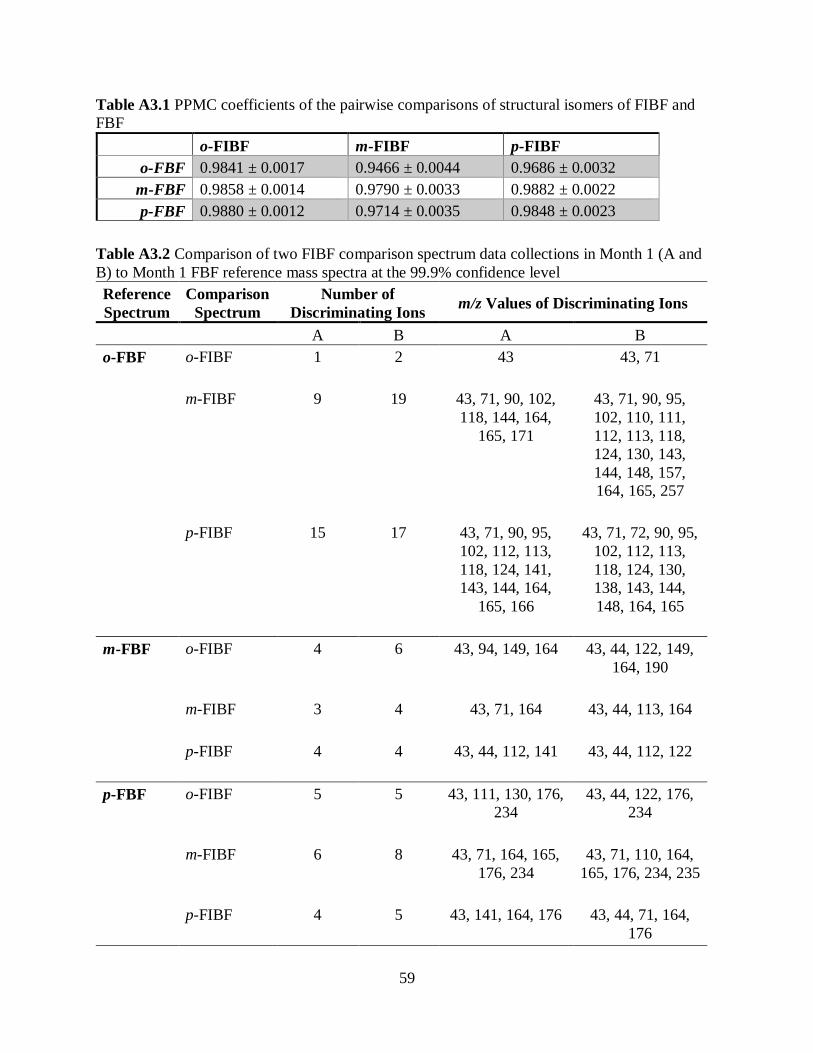
59

Table A3.1 PPMC coefficients of the pairwise comparisons of structural isomers of FIBF and

FBF

o-FIBF m-FIBF p-FIBF

o-FBF 0.9841 ± 0.0017 0.9466 ± 0.0044 0.9686 ± 0.0032

m-FBF 0.9858 ± 0.0014 0.9790 ± 0.0033 0.9882 ± 0.0022

p-FBF 0.9880 ± 0.0012 0.9714 ± 0.0035 0.9848 ± 0.0023

Table A3.2 Comparison of two FIBF comparison spectrum data collections in Month 1 (A and

B) to Month 1 FBF reference mass spectra at the 99.9% confidence level

Reference

Spectrum

Comparison

Spectrum

Number of


A B A B

o-FBF o-FIBF

1 2 43 43, 71

m-FIBF 9

19 43, 71, 90, 102,

118, 144, 164,

165, 171

43, 71, 90, 95,

102, 110, 111,

112, 113, 118,

124, 130, 143,

144, 148, 157,

164, 165, 257

p-FIBF 15 17 43, 71, 90, 95,

102, 112, 113,

118, 124, 141,

143, 144, 164,

165, 166

43, 71, 72, 90, 95,

102, 112, 113,

118, 124, 130,

138, 143, 144,

148, 164, 165

m-FBF o-FIBF 4

6 43, 94, 149, 164 43, 44, 122, 149,

164, 190

m-FIBF

3 4 43, 71, 164 43, 44, 113, 164

p-FIBF 4 4 43, 44, 112, 141 43, 44, 112, 122

p-FBF o-FIBF

5 5 43, 111, 130, 176,

234

43, 44, 122, 176,

234

m-FIBF

6 8 43, 71, 164, 165,

176, 234

43, 71, 110, 164,

165, 176, 234, 235

p-FIBF

4 5 43, 141, 164, 176 43, 44, 71, 164,

176

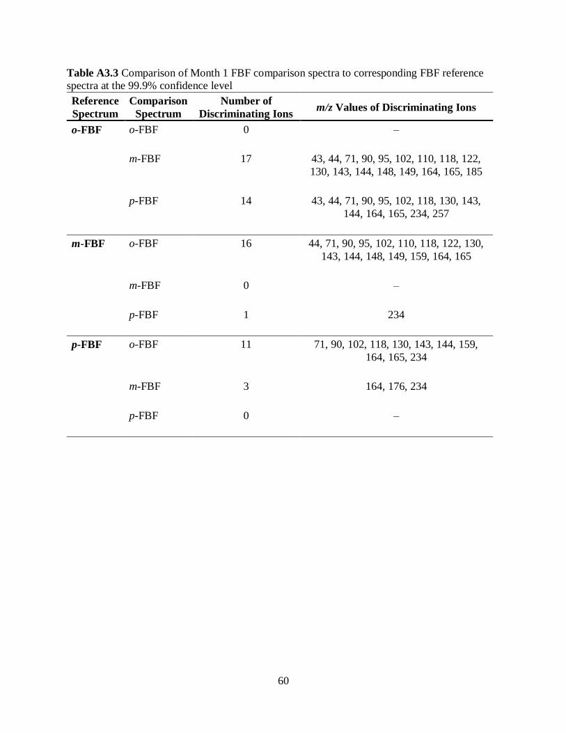
60

Table A3.3 Comparison of Month 1 FBF comparison spectra to corresponding FBF reference


Reference

Spectrum

Comparison

Spectrum

Number of


o-FBF o-FBF

0 –

m-FBF

17 43, 44, 71, 90, 95, 102, 110, 118, 122,

130, 143, 144, 148, 149, 164, 165, 185

p-FBF 14 43, 44, 71, 90, 95, 102, 118, 130, 143,

144, 164, 165, 234, 257

m-FBF o-FBF

16 44, 71, 90, 95, 102, 110, 118, 122, 130,

143, 144, 148, 149, 159, 164, 165

m-FBF

0 –

p-FBF

1 234

p-FBF o-FBF

11 71, 90, 102, 118, 130, 143, 144, 159,

164, 165, 234

m-FBF

3 164, 176, 234

p-FBF

0 –

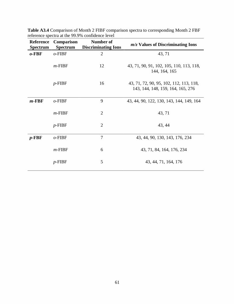
61


reference spectra at the 99.9% confidence level

Reference

Spectrum

Comparison

Spectrum

Number of


o-FBF o-FIBF

2 43, 71

m-FIBF

12 43, 71, 90, 91, 102, 105, 110, 113, 118,

144, 164, 165

p-FIBF 16 43, 71, 72, 90, 95, 102, 112, 113, 118,

143, 144, 148, 159, 164, 165, 276

m-FBF o-FIBF

9 43, 44, 90, 122, 130, 143, 144, 149, 164

m-FIBF

2 43, 71

p-FIBF

2 43, 44

p-FBF o-FIBF

7 43, 44, 90, 130, 143, 176, 234

m-FIBF

6 43, 71, 84, 164, 176, 234

p-FIBF

5 43, 44, 71, 164, 176

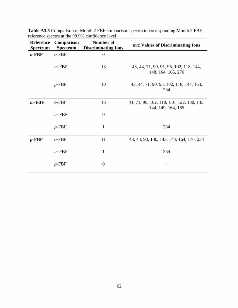
62



Reference

Spectrum

Comparison

Spectrum

Number of


o-FBF o-FBF

0 –

m-FBF

13 43, 44, 71, 90, 91, 95, 102, 118, 144,

148, 164, 165, 276

p-FBF 10 43, 44, 71, 90, 95, 102, 118, 144, 164,

234

m-FBF o-FBF

13 44, 71, 90, 102, 110, 118, 122, 130, 143,

144, 149, 164, 165

m-FBF

0 –

p-FBF

1 234

p-FBF o-FBF

11 43, 44, 90, 130, 143, 144, 164, 176, 234

m-FBF

1 234

p-FBF

0 –

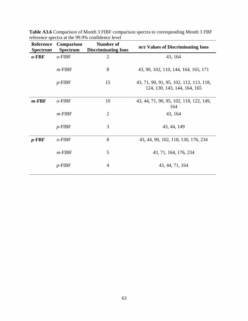
63



Reference

Spectrum

Comparison

Spectrum

Number of


o-FBF o-FIBF

2 43, 164

m-FIBF

8 43, 90, 102, 110, 144, 164, 165, 171

p-FIBF 15 43, 71, 90, 91, 95, 102, 112, 113, 118,

124, 130, 143, 144, 164, 165

m-FBF o-FIBF

10 43, 44, 71, 90, 95, 102, 118, 122, 149,

164

m-FIBF

2 43, 164

p-FIBF

3 43, 44, 149

p-FBF o-FIBF

8 43, 44, 90, 102, 118, 130, 176, 234

m-FIBF

5 43, 71, 164, 176, 234

p-FIBF

4 43, 44, 71, 164

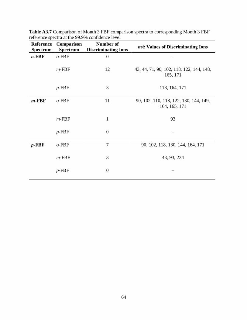
64



Reference

Spectrum

Comparison

Spectrum

Number of


o-FBF o-FBF

0 –

m-FBF

12 43, 44, 71, 90, 102, 118, 122, 144, 148,

165, 171

p-FBF 3 118, 164, 171

m-FBF o-FBF

11 90, 102, 110, 118, 122, 130, 144, 149,

164, 165, 171

m-FBF

1 93

p-FBF

0 –

p-FBF o-FBF

7 90, 102, 118, 130, 144, 164, 171

m-FBF

3 43, 93, 234

p-FBF

0 –

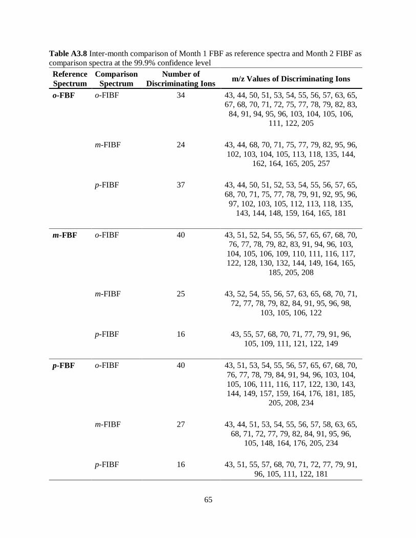
65

Table A3.8 Inter-month comparison of Month 1 FBF as reference spectra and Month 2 FIBF as


Reference

Spectrum

Comparison

Spectrum

Number of


o-FBF o-FIBF

34 43, 44, 50, 51, 53, 54, 55, 56, 57, 63, 65,

67, 68, 70, 71, 72, 75, 77, 78, 79, 82, 83,

84, 91, 94, 95, 96, 103, 104, 105, 106,

111, 122, 205

m-FIBF

24 43, 44, 68, 70, 71, 75, 77, 79, 82, 95, 96,

102, 103, 104, 105, 113, 118, 135, 144,

162, 164, 165, 205, 257

p-FIBF 37 43, 44, 50, 51, 52, 53, 54, 55, 56, 57, 65,

68, 70, 71, 75, 77, 78, 79, 91, 92, 95, 96,

97, 102, 103, 105, 112, 113, 118, 135,

143, 144, 148, 159, 164, 165, 181

m-FBF o-FIBF

40 43, 51, 52, 54, 55, 56, 57, 65, 67, 68, 70,

76, 77, 78, 79, 82, 83, 91, 94, 96, 103,

104, 105, 106, 109, 110, 111, 116, 117,

122, 128, 130, 132, 144, 149, 164, 165,

185, 205, 208

m-FIBF

25 43, 52, 54, 55, 56, 57, 63, 65, 68, 70, 71,

72, 77, 78, 79, 82, 84, 91, 95, 96, 98,

103, 105, 106, 122

p-FIBF

16 43, 55, 57, 68, 70, 71, 77, 79, 91, 96,

105, 109, 111, 121, 122, 149

p-FBF o-FIBF

40 43, 51, 53, 54, 55, 56, 57, 65, 67, 68, 70,

76, 77, 78, 79, 84, 91, 94, 96, 103, 104,

105, 106, 111, 116, 117, 122, 130, 143,

144, 149, 157, 159, 164, 176, 181, 185,

205, 208, 234

m-FIBF

27 43, 44, 51, 53, 54, 55, 56, 57, 58, 63, 65,

68, 71, 72, 77, 79, 82, 84, 91, 95, 96,

105, 148, 164, 176, 205, 234

p-FIBF

16 43, 51, 55, 57, 68, 70, 71, 72, 77, 79, 91,

96, 105, 111, 122, 181

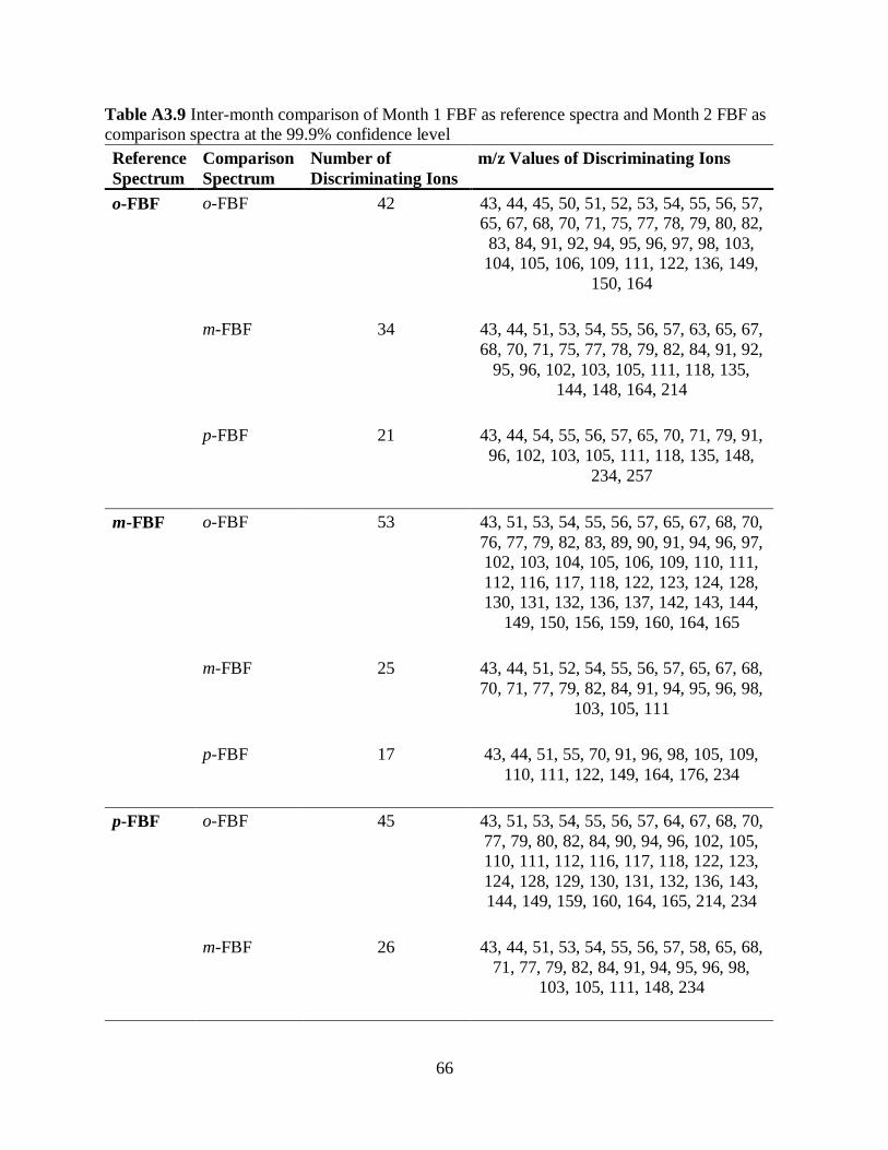
66

Table A3.9 Inter-month comparison of Month 1 FBF as reference spectra and Month 2 FBF as


Reference

Spectrum

Comparison

Spectrum

Number of

Discriminating Ions


o-FBF o-FBF

42 43, 44, 45, 50, 51, 52, 53, 54, 55, 56, 57,

65, 67, 68, 70, 71, 75, 77, 78, 79, 80, 82,

83, 84, 91, 92, 94, 95, 96, 97, 98, 103,

104, 105, 106, 109, 111, 122, 136, 149,

150, 164

m-FBF

34 43, 44, 51, 53, 54, 55, 56, 57, 63, 65, 67,

68, 70, 71, 75, 77, 78, 79, 82, 84, 91, 92,

95, 96, 102, 103, 105, 111, 118, 135,

144, 148, 164, 214

p-FBF 21 43, 44, 54, 55, 56, 57, 65, 70, 71, 79, 91,

96, 102, 103, 105, 111, 118, 135, 148,

234, 257

m-FBF o-FBF

53 43, 51, 53, 54, 55, 56, 57, 65, 67, 68, 70,

76, 77, 79, 82, 83, 89, 90, 91, 94, 96, 97,

102, 103, 104, 105, 106, 109, 110, 111,

112, 116, 117, 118, 122, 123, 124, 128,

130, 131, 132, 136, 137, 142, 143, 144,

149, 150, 156, 159, 160, 164, 165

m-FBF

25 43, 44, 51, 52, 54, 55, 56, 57, 65, 67, 68,

70, 71, 77, 79, 82, 84, 91, 94, 95, 96, 98,

103, 105, 111

p-FBF

17 43, 44, 51, 55, 70, 91, 96, 98, 105, 109,

110, 111, 122, 149, 164, 176, 234

p-FBF o-FBF

45 43, 51, 53, 54, 55, 56, 57, 64, 67, 68, 70,

77, 79, 80, 82, 84, 90, 94, 96, 102, 105,

110, 111, 112, 116, 117, 118, 122, 123,

124, 128, 129, 130, 131, 132, 136, 143,

144, 149, 159, 160, 164, 165, 214, 234

m-FBF

26 43, 44, 51, 53, 54, 55, 56, 57, 58, 65, 68,

71, 77, 79, 82, 84, 91, 94, 95, 96, 98,

103, 105, 111, 148, 234

67

REFERENCES

68

REFERENCES

(1) Pierzynski, H. G.; Neubauer, L.; Choi, C.; Franckowski, R.; Augustin, Iula, D. M. Tips for

Interpreting GC-MS Fragmentation of Unknown Substituted Fentanyls. Cayman Currents.

2017, 28, 1-3

(2) Jariwala, F. B.; Figus, M.; Attygalle, A. B. Ortho Effect in Electron Ionization Mass

Spectrometry of N-Acylanilines Bearing a Proximal Halo Substituent. Journal of American

Society for Mass Spectrometry 2008, 19, 1114-1118

69

IV. Further Investigation of a Refined Approach to Predict Standard Deviation

While the overall results of the intra-month comparisons of the fluoroisobutyryl fentanyl

(FIBF) and fluorobutyryl fentanyl (FBF) isomers in Months 1-3 led to successful association and

discrimination in most cases, there were some comparisons that resulted in incorrect associations

(false positives) and incorrect discriminations (false negatives). Additionally, the inter-month

comparisons between Month 1 and Month 2 resulted in no association and discriminations with

many ions responsible. Following the results demonstrated in Chapter 3, further investigation

into the regression plots was made in order to refine the method of standard deviation prediction

to more accurately model the response of the electron multiplier and increase confidence in the

statistical comparisons of the FIBF and FBF isomers.

4.1 Investigation of Regression Lines

In order to perform the statistical comparisons of FIBF and FBF isomers, a mathematical

model was previously created to predict the standard deviations used in the t-test calculation.

This method of standard deviation prediction is based upon the counting statistics of the electron

multiplier response (Sections 1.3 and 2.3). Using the spectral data from the set of normal (n-)

alkanes analyzed in replicate and at different concentrations, regression plots were generated for

each month of analysis as shown in Figure 4.1 A-C. The slopes ranged from 0.6468 to 0.7190

and the coefficient of linear fit (R2) ranged from 0.86 to 0.91.

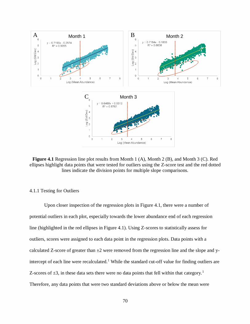
70

Figure 4.1 Regression line plot results from Month 1 (A), Month 2 (B), and Month 3 (C). Red

ellipses highlight data points that were tested for outliers using the Z-score test and the red dotted

lines indicate the division points for multiple slope comparisons.

4.1.1 Testing for Outliers

Upon closer inspection of the regression plots in Figure 4.1, there were a number of

potential outliers in each plot, especially towards the lower abundance end of each regression

line (highlighted in the red ellipses in Figure 4.1). Using Z-scores to statistically assess for

outliers, scores were assigned to each data point in the regression plots. Data points with a

calculated Z-score of greater than ±2 were removed from the regression line and the slope and y-

intercept of each line were recalculated.1 While the standard cut-off value for finding outliers are

Z-scores of ±3, in these data sets there were no data points that fell within that category.1

Therefore, any data points that were two standard deviations above or below the mean were

Month 1 Month 2

Month 3

A B

C

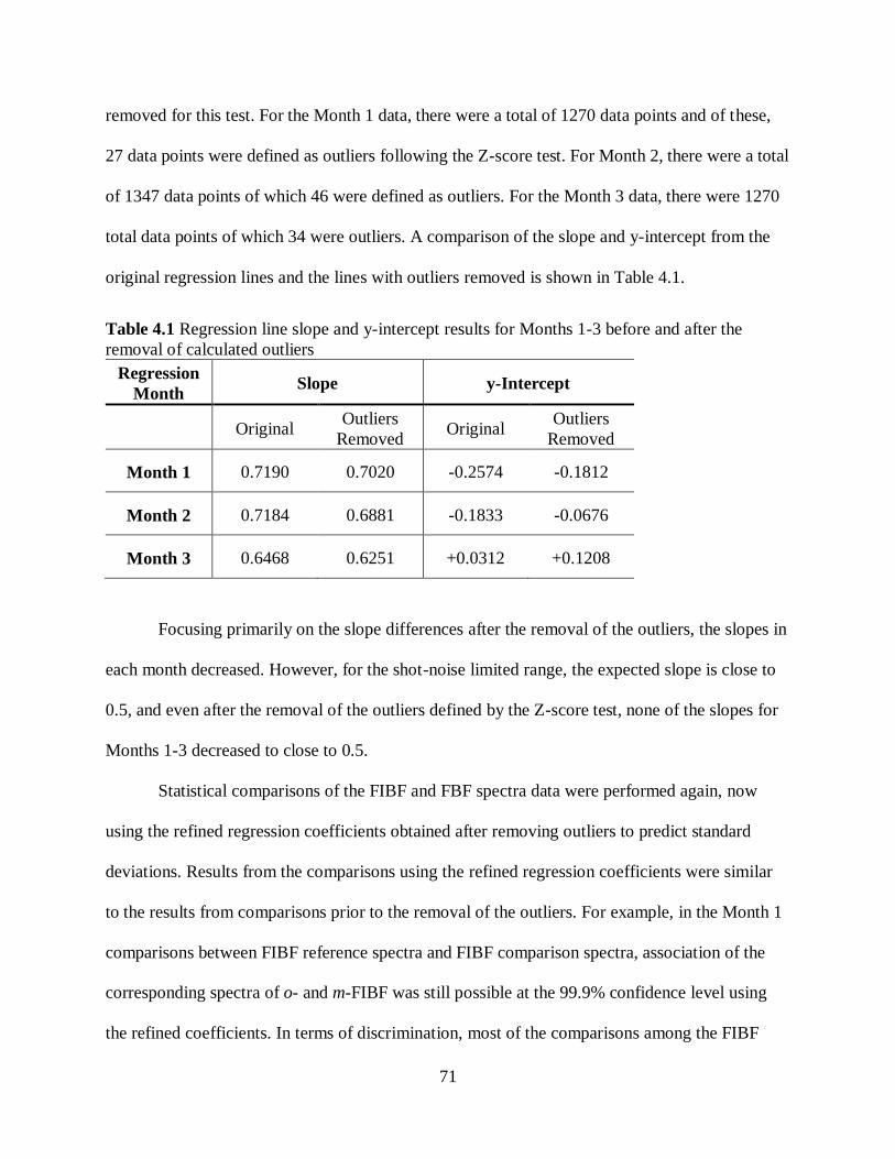
71

removed for this test. For the Month 1 data, there were a total of 1270 data points and of these,

27 data points were defined as outliers following the Z-score test. For Month 2, there were a total

of 1347 data points of which 46 were defined as outliers. For the Month 3 data, there were 1270

total data points of which 34 were outliers. A comparison of the slope and y-intercept from the

original regression lines and the lines with outliers removed is shown in Table 4.1.

Table 4.1 Regression line slope and y-intercept results for Months 1-3 before and after the

removal of calculated outliers

Regression

Month Slope y-Intercept

Original

Outliers

Removed Original

Outliers

Removed

Month 1 0.7190 0.7020 -0.2574 -0.1812

Month 2 0.7184 0.6881 -0.1833 -0.0676

Month 3 0.6468 0.6251 +0.0312 +0.1208

Focusing primarily on the slope differences after the removal of the outliers, the slopes in

each month decreased. However, for the shot-noise limited range, the expected slope is close to

0.5, and even after the removal of the outliers defined by the Z-score test, none of the slopes for

Months 1-3 decreased to close to 0.5.

Statistical comparisons of the FIBF and FBF spectra data were performed again, now

using the refined regression coefficients obtained after removing outliers to predict standard

deviations. Results from the comparisons using the refined regression coefficients were similar

to the results from comparisons prior to the removal of the outliers. For example, in the Month 1

comparisons between FIBF reference spectra and FIBF comparison spectra, association of the

corresponding spectra of o- and m-FIBF was still possible at the 99.9% confidence level using

the refined coefficients. In terms of discrimination, most of the comparisons among the FIBF

72

isomers resulted in the same number and identities of discriminating ions. There were two

instances in which the number of discriminating ions varied. The comparison between the p-

FIBF comparison spectrum and the o-FIBF reference spectra resulted in 10 discriminating ions

when using the original regression coefficients and only 9 ions when using the refined

coefficients after outlier removal. The one ion that was different was m/z 143, which had a tcalc

value of 13.169 in the original comparison and a tcalc value of 12.589 in the refined comparison

which were compared to a tcrit value of 12.924 in both situations.

The o-FIBF comparison spectrum to the m-FIBF reference spectra also resulted in a

different number of discriminating ions with the removal of outliers from the regression line. In

the original comparison, there were only 8 discriminating ions, but in the comparison using the

refined regression coefficients, there were 9 discriminating ions. The ion that was present in the

refined comparison but not the original one was m/z 102, which had tcalc values of 21.805 and

21.187 in the original and refined comparisons, respectively. However, in this case, the tcrit

values changed between the two comparisons – from 31.599 in the original comparison to 12.924

in the comparison after removing outliers. Therefore, the differences in regression line

coefficients pre- and post-outlier removal did affect the predicted standard deviations of the

reference spectra and comparison spectra slightly as well as changing the degrees of freedom

results, which in-turn affected the tcalc and tcrit values of each m/z value in the spectra being

statistically compared. However, these changes did not affect the overall results. No comparison

between FIBF or FBF isomers resulted in a different overall result of association or

discrimination due to the removal of the outliers. In addition, the differences in the numbers of

discriminating ions did not vary greatly between the two types of comparisons, as shown in the

73

Month 1 comparison example. Results from all other comparisons can be found in Appendix

Tables A4.1 – A4.12.

Because of the similar results, all comparisons moving forward were performed using the

original regression coefficients, without the extra step of removing outliers. This is also a simpler

and more streamlined approach that is more practical for applying the method to casework in a

forensic laboratory.

4.1.2 Investigating Different Linear Regions Within Each Plot

Upon further inspection of the regression lines for each month, it appeared that within

each plot there may be two linear regions with different slopes, which are indicated on either side

of the red dotted lines in Figure 4.1. The first region includes a lower abundance region in which

the standard deviation is proportional to abundance in a manner similar to that expected for shot-

noise limits with a slope closer to 0.5. The second region includes a higher abundance portion

expected for signal-to-noise scaling directly with signal with a slope closer to 1.0 (proportional

noise region). Using two slopes, or a segmented regression line, to more accurately predict the

standard deviation as a function of abundance could result in more accurate t-values, and

therefore, more accurate comparisons. Based on visual inspection of each regression line, the

abundance value to use as the breakpoint was manually selected, which is denoted by the red

dotted lines in Figures 4.1 and 4.2.

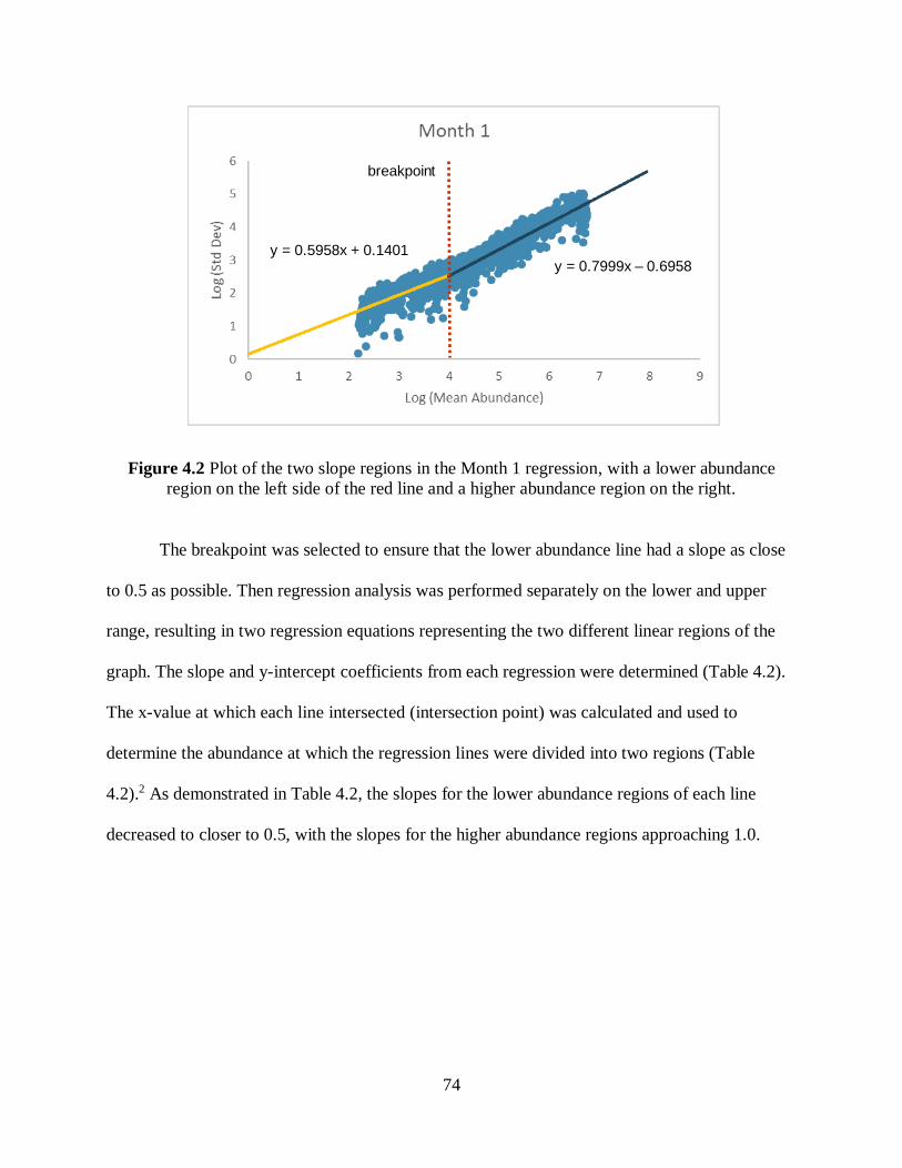
74

Figure 4.2 Plot of the two slope regions in the Month 1 regression, with a lower abundance

region on the left side of the red line and a higher abundance region on the right.

The breakpoint was selected to ensure that the lower abundance line had a slope as close

to 0.5 as possible. Then regression analysis was performed separately on the lower and upper

range, resulting in two regression equations representing the two different linear regions of the

graph. The slope and y-intercept coefficients from each regression were determined (Table 4.2).

The x-value at which each line intersected (intersection point) was calculated and used to

determine the abundance at which the regression lines were divided into two regions (Table

4.2).2 As demonstrated in Table 4.2, the slopes for the lower abundance regions of each line

decreased to closer to 0.5, with the slopes for the higher abundance regions approaching 1.0.

y = 0.5958x + 0.1401y = 0.7999x – 0.6958

breakpoint

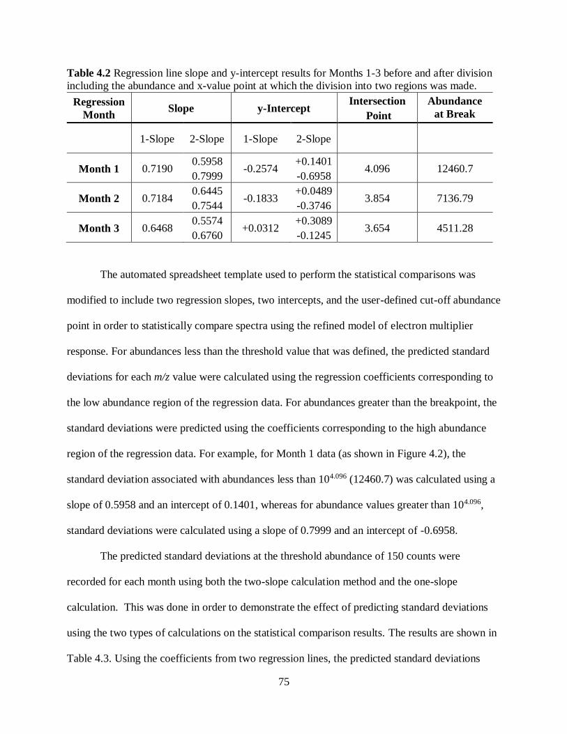
75

Table 4.2 Regression line slope and y-intercept results for Months 1-3 before and after division

including the abundance and x-value point at which the division into two regions was made.

Regression

Month Slope y-Intercept

Intersection

Point

Abundance

at Break

1-Slope 2-Slope 1-Slope 2-Slope

Month 1 0.7190 0.5958

0.7999 -0.2574

+0.1401

-0.6958 4.096 12460.7

Month 2 0.7184 0.6445

0.7544 -0.1833

+0.0489

-0.3746 3.854 7136.79

Month 3 0.6468 0.5574

0.6760 +0.0312

+0.3089

-0.1245 3.654 4511.28

The automated spreadsheet template used to perform the statistical comparisons was

modified to include two regression slopes, two intercepts, and the user-defined cut-off abundance

point in order to statistically compare spectra using the refined model of electron multiplier

response. For abundances less than the threshold value that was defined, the predicted standard

deviations for each m/z value were calculated using the regression coefficients corresponding to

the low abundance region of the regression data. For abundances greater than the breakpoint, the

standard deviations were predicted using the coefficients corresponding to the high abundance

region of the regression data. For example, for Month 1 data (as shown in Figure 4.2), the

standard deviation associated with abundances less than 104.096 (12460.7) was calculated using a

slope of 0.5958 and an intercept of 0.1401, whereas for abundance values greater than 104.096,

standard deviations were calculated using a slope of 0.7999 and an intercept of -0.6958.

The predicted standard deviations at the threshold abundance of 150 counts were

recorded for each month using both the two-slope calculation method and the one-slope

calculation. This was done in order to demonstrate the effect of predicting standard deviations

using the two types of calculations on the statistical comparison results. The results are shown in

Table 4.3. Using the coefficients from two regression lines, the predicted standard deviations

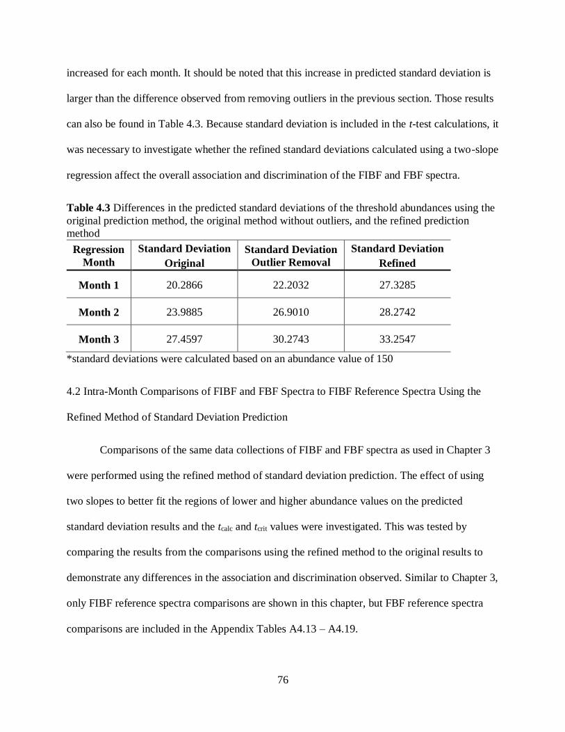
76

increased for each month. It should be noted that this increase in predicted standard deviation is

larger than the difference observed from removing outliers in the previous section. Those results

can also be found in Table 4.3. Because standard deviation is included in the t-test calculations, it

was necessary to investigate whether the refined standard deviations calculated using a two-slope

regression affect the overall association and discrimination of the FIBF and FBF spectra.

Table 4.3 Differences in the predicted standard deviations of the threshold abundances using the

original prediction method, the original method without outliers, and the refined prediction

method

Regression

Month

Standard Deviation

Original

Standard Deviation

Outlier Removal

Standard Deviation

Refined

Month 1 20.2866 22.2032 27.3285

Month 2 23.9885 26.9010 28.2742

Month 3 27.4597 30.2743 33.2547

*standard deviations were calculated based on an abundance value of 150

4.2 Intra-Month Comparisons of FIBF and FBF Spectra to FIBF Reference Spectra Using the

Refined Method of Standard Deviation Prediction

Comparisons of the same data collections of FIBF and FBF spectra as used in Chapter 3

were performed using the refined method of standard deviation prediction. The effect of using

two slopes to better fit the regions of lower and higher abundance values on the predicted

standard deviation results and the tcalc and tcrit values were investigated. This was tested by

comparing the results from the comparisons using the refined method to the original results to

demonstrate any differences in the association and discrimination observed. Similar to Chapter 3,

only FIBF reference spectra comparisons are shown in this chapter, but FBF reference spectra

comparisons are included in the Appendix Tables A4.13 – A4.19.

77

4.2.1 Month 1 FIBF and FBF Spectra Compared to Month 1 FIBF Reference Spectra Using the

Refined Method to Predict Standard Deviation

The FIBF comparison spectra collected in Month 1 were compared to the corresponding

Month 1 FIBF reference spectra using the refined method to predict standard deviation. As

mentioned in Chapter 3, two sets of Month 1 comparison spectra were collected (Month 1A and

Month 1B) to demonstrate the ability of the method to statistically compare spectra analyzed on

different days to the same reference spectra under equivalent conditions and still yield similar

results. Table 4.4 shows the results for the comparison between Month 1A comparison spectra to

corresponding FIBF reference spectra for both the original comparisons and the refined method

comparisons. While the number of discriminating ions was different between the two

comparisons, the overall results, whether association or discrimination was made, were

unchanged. Corresponding spectra of o-FIBF, m-FIBF, and p-FIBF were statistically associated

at the 99.9% confidence level when using the refined method with the same maximum and

minimum random-match probabilities (Pmax and Pmin) for each comparison as observed during

the original comparisons.

In terms of discrimination, the Month 1A comparison FIBF spectra were still

discriminated from the FIBF reference spectra in all cases (Table 4.4) at the 99.9% confidence

level. However, the refined method resulted in a higher number of discriminating ions in all

cases except for the comparison between p-FIBF reference spectra and the o-FIBF comparison

spectrum, where the number of ions remained the same (3). In most of these instances, the m/z

values of the discriminating ions remained constant between the original comparisons and the

comparisons using the refined method, with the refined method only identifying additional

discriminating ions.

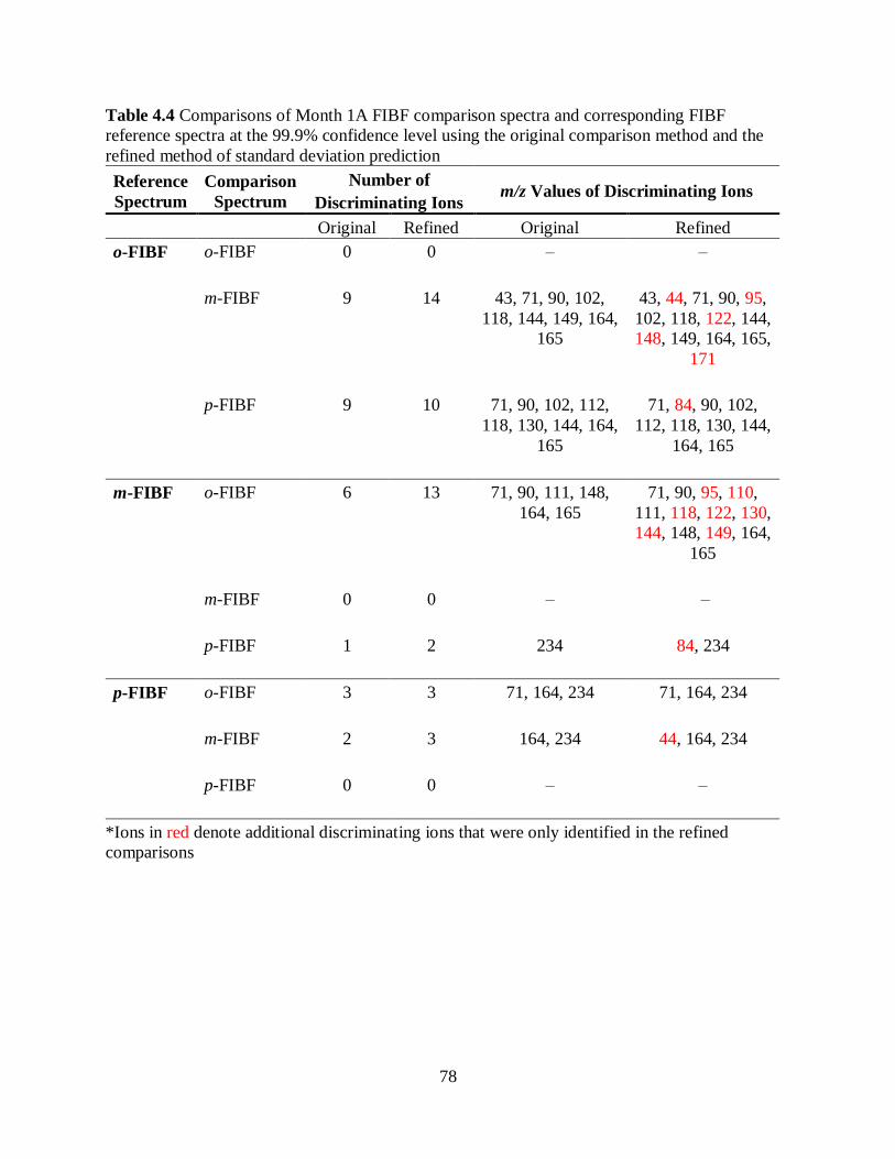
78

Table 4.4 Comparisons of Month 1A FIBF comparison spectra and corresponding FIBF


refined method of standard deviation prediction

Reference

Spectrum

Comparison

Spectrum

Number of


Original Refined Original Refined

o-FIBF o-FIBF

0 0 – –

m-FIBF 9 14 43, 71, 90, 102,

118, 144, 149, 164,

165

43, 44, 71, 90, 95,

102, 118, 122, 144,

148, 149, 164, 165,

171

p-FIBF 9 10 71, 90, 102, 112,

118, 130, 144, 164,

165

71, 84, 90, 102,

112, 118, 130, 144,

164, 165

m-FIBF o-FIBF 6 13 71, 90, 111, 148,

164, 165

71, 90, 95, 110,

111, 118, 122, 130,

144, 148, 149, 164,

165

m-FIBF

0 0 – –

p-FIBF 1 2 234 84, 234

p-FIBF o-FIBF

3 3 71, 164, 234 71, 164, 234

m-FIBF

2 3 164, 234 44, 164, 234

p-FIBF

0 0 – –

*Ions in red denote additional discriminating ions that were only identified in the refined

comparisons

79

The refined method comparisons involving o-FIBF as either the comparison spectrum or

reference spectra resulted in new common discriminating ions including m/z 95 and m/z 122. In

the case of m/z 95, this ion was present as a new discriminating ion for the comparisons of o-

FIBF to m-FIBF. In both situations, the predicted standard deviations of the reference and

comparison spectra for that ion decreased when using the refined method. For example, in the

comparison of the m-FIBF comparison spectrum to the o-FIBF reference spectra, the predicted

standard deviation of m/z 95 in the m-FIBF comparison spectrum was 3.03x10-3 in the original

comparison and 2.50x10-3 in the refined comparison. The effect of the decrease in predicted

standard deviations of that ion resulted in an increase in the tcalc value without also increasing the

tcrit value. In the original comparison, the tcalc value was 12.645 compared to a tcrit value of

12.924. Using the refined method, the tcalc value increased to 15.044, which was greater than the

tcrit value and the null hypothesis was no longer accepted at that m/z value. This resulted in an

additional discriminating ion. This was also the case for the ion at m/z 122, where the predicted

standard deviations in both the comparison and reference spectra decreased, which increased the

tcalc value to greater than the tcrit value. The comparisons using the refined method that involved

m-FIBF contained a new discriminating ion at m/z 44, where the tcalc value increased from 12.368

to 13.510. The new discriminating ion observed when comparing p-FIBF using the refined

method was m/z 84, where the tcalc value increased from 10.938 to 13.470.

Comparisons of Month 1B FIBF comparison spectra to corresponding Month 1 reference

spectra were also performed using the refined method and results were related to the one-slope

comparisons in Table 4.5. As with the Month 1A comparisons above, similar overall results of

association and discrimination were observed between the two different types of comparisons.

Corresponding spectra of o-FIBF and m-FIBF were associated at the 99.9% confidence level

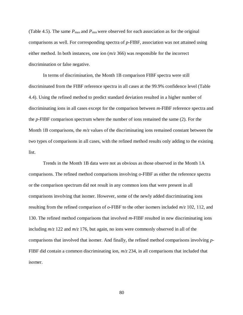
80

(Table 4.5). The same Pmax and Pmin were observed for each association as for the original

comparisons as well. For corresponding spectra of p-FIBF, association was not attained using

either method. In both instances, one ion (m/z 366) was responsible for the incorrect

discrimination or false negative.

In terms of discrimination, the Month 1B comparison FIBF spectra were still

discriminated from the FIBF reference spectra in all cases at the 99.9% confidence level (Table

4.4). Using the refined method to predict standard deviation resulted in a higher number of

discriminating ions in all cases except for the comparison between m-FIBF reference spectra and

the p-FIBF comparison spectrum where the number of ions remained the same (2). For the

Month 1B comparisons, the m/z values of the discriminating ions remained constant between the

two types of comparisons in all cases, with the refined method results only adding to the existing

list.

Trends in the Month 1B data were not as obvious as those observed in the Month 1A

comparisons. The refined method comparisons involving o-FIBF as either the reference spectra

or the comparison spectrum did not result in any common ions that were present in all

comparisons involving that isomer. However, some of the newly added discriminating ions

resulting from the refined comparison of o-FIBF to the other isomers included m/z 102, 112, and

130. The refined method comparisons that involved m-FIBF resulted in new discriminating ions

including m/z 122 and m/z 176, but again, no ions were commonly observed in all of the

comparisons that involved that isomer. And finally, the refined method comparisons involving p-

FIBF did contain a common discriminating ion, m/z 234, in all comparisons that included that

isomer.

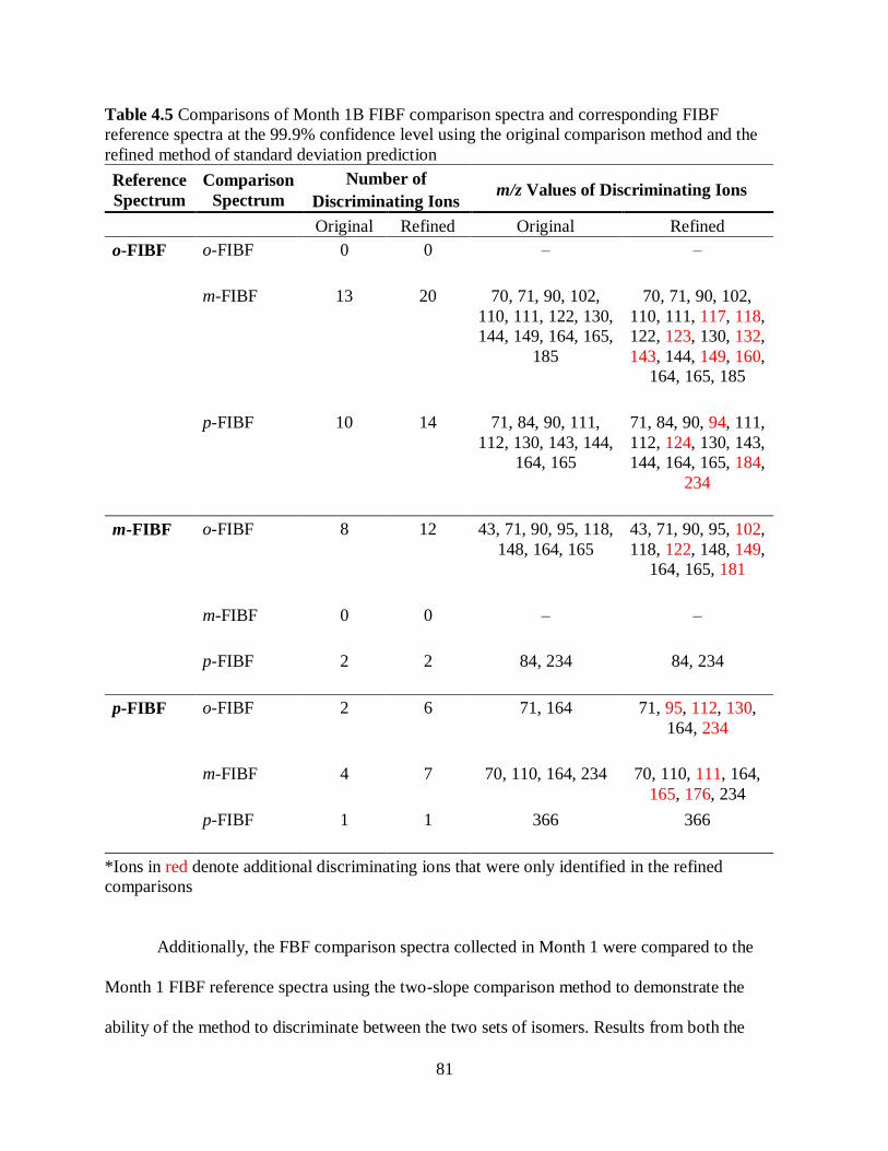
81

Table 4.5 Comparisons of Month 1B FIBF comparison spectra and corresponding FIBF



Reference

Spectrum

Comparison

Spectrum

Number of



o-FIBF o-FIBF

0 0 – –

m-FIBF 13 20 70, 71, 90, 102,

110, 111, 122, 130,

144, 149, 164, 165,

185

70, 71, 90, 102,

110, 111, 117, 118,

122, 123, 130, 132,

143, 144, 149, 160,

164, 165, 185

p-FIBF 10 14 71, 84, 90, 111,

112, 130, 143, 144,

164, 165

71, 84, 90, 94, 111,

112, 124, 130, 143,

144, 164, 165, 184,

234

m-FIBF o-FIBF 8 12 43, 71, 90, 95, 118,

148, 164, 165

43, 71, 90, 95, 102,

118, 122, 148, 149,

164, 165, 181

m-FIBF

0 0 – –

p-FIBF 2 2 84, 234 84, 234

p-FIBF o-FIBF

2 6 71, 164 71, 95, 112, 130,

164, 234

m-FIBF

4 7 70, 110, 164, 234 70, 110, 111, 164,

165, 176, 234

p-FIBF

1 1 366 366


comparisons

Additionally, the FBF comparison spectra collected in Month 1 were compared to the

Month 1 FIBF reference spectra using the two-slope comparison method to demonstrate the

ability of the method to discriminate between the two sets of isomers. Results from both the

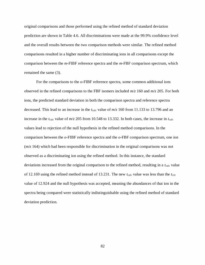
82

original comparisons and those performed using the refined method of standard deviation

prediction are shown in Table 4.6. All discriminations were made at the 99.9% confidence level

and the overall results between the two comparison methods were similar. The refined method

comparisons resulted in a higher number of discriminating ions in all comparisons except the

comparison between the m-FIBF reference spectra and the m-FBF comparison spectrum, which

remained the same (3).

For the comparisons to the o-FIBF reference spectra, some common additional ions

observed in the refined comparisons to the FBF isomers included m/z 160 and m/z 205. For both

ions, the predicted standard deviation in both the comparison spectra and reference spectra

decreased. This lead to an increase in the tcalc value of m/z 160 from 11.133 to 13.796 and an

increase in the tcalc value of m/z 205 from 10.548 to 13.332. In both cases, the increase in tcalc

values lead to rejection of the null hypothesis in the refined method comparisons. In the

comparison between the o-FIBF reference spectra and the o-FBF comparison spectrum, one ion

(m/z 164) which had been responsible for discrimination in the original comparisons was not

observed as a discriminating ion using the refined method. In this instance, the standard

deviations increased from the original comparison to the refined method, resulting in a tcalc value

of 12.169 using the refined method instead of 13.231. The new tcalc value was less than the tcrit

value of 12.924 and the null hypothesis was accepted, meaning the abundances of that ion in the

spectra being compared were statistically indistinguishable using the refined method of standard

deviation prediction.

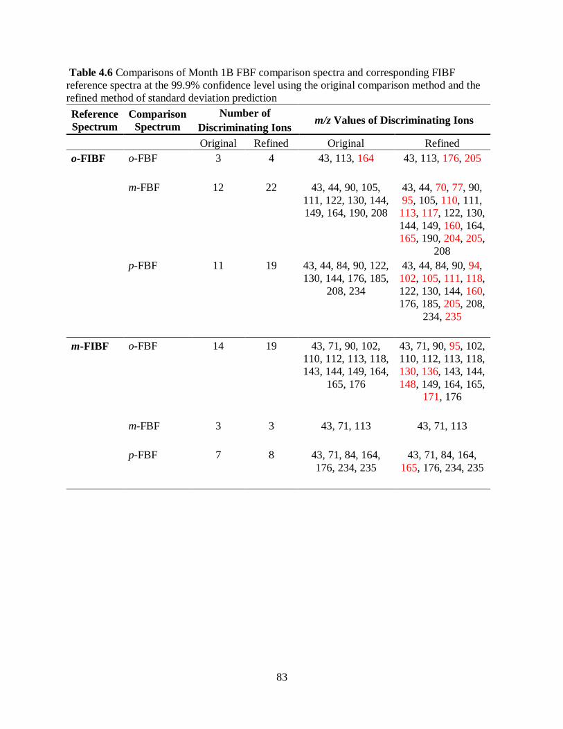
83

Table 4.6 Comparisons of Month 1B FBF comparison spectra and corresponding FIBF



Reference

Spectrum

Comparison

Spectrum

Number of



o-FIBF o-FBF

3 4 43, 113, 164 43, 113, 176, 205

m-FBF

12 22 43, 44, 90, 105,

111, 122, 130, 144,

149, 164, 190, 208

43, 44, 70, 77, 90,

95, 105, 110, 111,

113, 117, 122, 130,

144, 149, 160, 164,

165, 190, 204, 205,

208

p-FBF 11 19 43, 44, 84, 90, 122,

130, 144, 176, 185,

208, 234

43, 44, 84, 90, 94,

102, 105, 111, 118,

122, 130, 144, 160,

176, 185, 205, 208,

234, 235

m-FIBF o-FBF

14 19 43, 71, 90, 102,

110, 112, 113, 118,

143, 144, 149, 164,

165, 176

43, 71, 90, 95, 102,

110, 112, 113, 118,

130, 136, 143, 144,

148, 149, 164, 165,

171, 176

m-FBF

3 3 43, 71, 113 43, 71, 113

p-FBF

7 8 43, 71, 84, 164,

176, 234, 235

43, 71, 84, 164,

165, 176, 234, 235

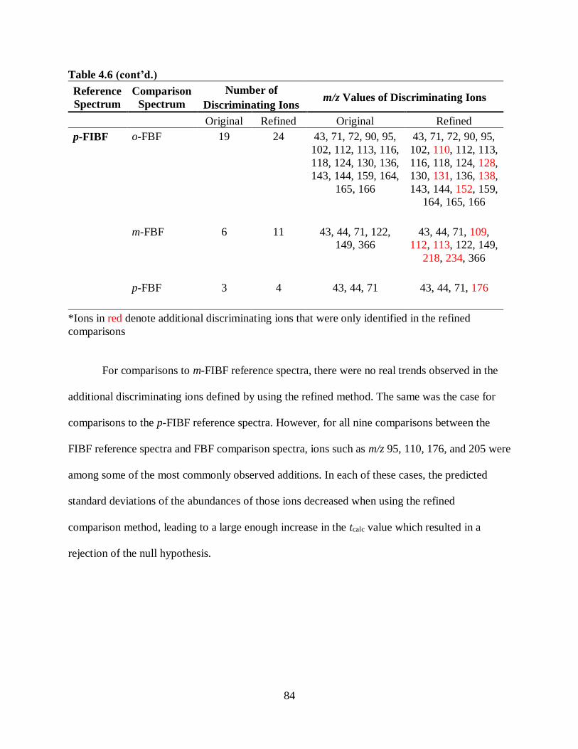
84


Reference

Spectrum

Comparison

Spectrum

Number of



p-FIBF o-FBF

19 24 43, 71, 72, 90, 95,

102, 112, 113, 116,

118, 124, 130, 136,

143, 144, 159, 164,

165, 166

43, 71, 72, 90, 95,

102, 110, 112, 113,

116, 118, 124, 128,

130, 131, 136, 138,

143, 144, 152, 159,

164, 165, 166

m-FBF

6 11 43, 44, 71, 122,

149, 366

43, 44, 71, 109,

112, 113, 122, 149,

218, 234, 366

p-FBF

3 4 43, 44, 71 43, 44, 71, 176


comparisons

For comparisons to m-FIBF reference spectra, there were no real trends observed in the

additional discriminating ions defined by using the refined method. The same was the case for

comparisons to the p-FIBF reference spectra. However, for all nine comparisons between the

FIBF reference spectra and FBF comparison spectra, ions such as m/z 95, 110, 176, and 205 were

among some of the most commonly observed additions. In each of these cases, the predicted

standard deviations of the abundances of those ions decreased when using the refined

comparison method, leading to a large enough increase in the tcalc value which resulted in a

rejection of the null hypothesis.

85



Comparisons were performed using the refined method of standard deviation prediction

on the Month 2 data involving FIBF reference spectra to corresponding FIBF comparison

spectra. Results were compared to the corresponding original comparisons as shown in Table

4.7. Overall, the results between the two types of comparisons were similar, with association at

the 99.9% confidence level for corresponding spectra of all o-, m-, and p-FIBF isomers with the

same Pmax and Pmin values in each instance as those observed from the original comparisons.

Each isomer of FIBF was also discriminated from the other two isomers at the 99.9% confidence

level using both types of comparisons.

In the comparisons using the refined method, a higher number of discriminating ions was

observed for the comparisons of the o-FIBF reference spectra to both m- and p-FIBF comparison

spectra and the p-FIBF reference spectra to the o-FIBF comparison spectrum (Table 4.7). All

other comparisons resulted in the same number and identity of observed discriminating ions

using each type of comparison. All cases that involved an increase in the number of

discriminating ions contained the same original discriminating ions.

Because many of the comparisons resulted in the same number of discriminating ions,

fewer trends were observed. Comparisons involving o-FIBF resulted in a common additional ion

at m/z 144. The predicted standard deviations of that ion decreased, leading to an increase in the

tcalc value from 12.139 to 13.379, while the tcrit value remained the same at 12.924.

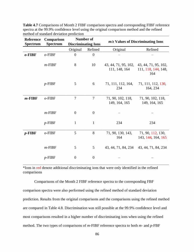
86



method of standard deviation prediction

Reference

Spectrum

Comparison

Spectrum

Number of



o-FIBF o-FIBF

0 0 – –

m-FIBF 8 10 43, 44, 71, 95, 102,

111, 148, 164

43, 44, 71, 95, 102,

111, 118, 144, 148,

164

p-FIBF 5 6 71, 111, 112, 164,

234

71, 111, 112, 130,

164, 234

m-FIBF o-FIBF 7 7 71, 90, 102, 118,

149, 164, 165

71, 90, 102, 118,

149, 164, 165

m-FIBF

0 0 – –

p-FIBF 1 1 234

234

p-FIBF o-FIBF

5 8 71, 90, 130, 143,

164

71, 90, 112, 130,

143, 144, 164, 165

m-FIBF

5 5 43, 44, 71, 84, 234 43, 44, 71, 84, 234

p-FIBF

0 0 – –


comparisons

Comparisons of the Month 2 FIBF reference spectra to the corresponding FBF

comparison spectra were also performed using the refined method of standard deviation

prediction. Results from the original comparisons and the comparisons using the refined method

are compared in Table 4.8. Discrimination was still possible at the 99.9% confidence level and

most comparisons resulted in a higher number of discriminating ions when using the refined

method. The two types of comparisons of m-FIBF reference spectra to both m- and p-FBF

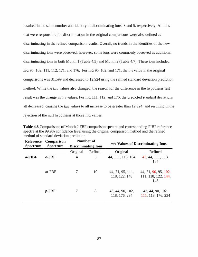
87

resulted in the same number and identity of discriminating ions, 3 and 5, respectively. All ions

that were responsible for discrimination in the original comparisons were also defined as

discriminating in the refined comparison results. Overall, no trends in the identities of the new

discriminating ions were observed; however, some ions were commonly observed as additional

discriminating ions in both Month 1 (Table 4.5) and Month 2 (Table 4.7). These ions included

m/z 95, 102, 111, 112, 171, and 176. For m/z 95, 102, and 171, the tcrit value in the original

comparisons was 31.599 and decreased to 12.924 using the refined standard deviation prediction

method. While the tcalc values also changed, the reason for the difference in the hypothesis test

result was the change in tcrit values. For m/z 111, 112, and 176, the predicted standard deviations

all decreased, causing the tcalc values to all increase to be greater than 12.924, and resulting in the

rejection of the null hypothesis at those m/z values.




Reference

Spectrum

Comparison

Spectrum

Number of



o-FIBF o-FBF

4 5 44, 111, 113, 164 43, 44, 111, 113,

164

m-FBF

7 10 44, 71, 95, 111,

118, 122, 148

44, 71, 90, 95, 102,

111, 118, 122, 144,

148

p-FBF 7 8 43, 44, 90, 102,

118, 176, 234

43, 44, 90, 102,

111, 118, 176, 234

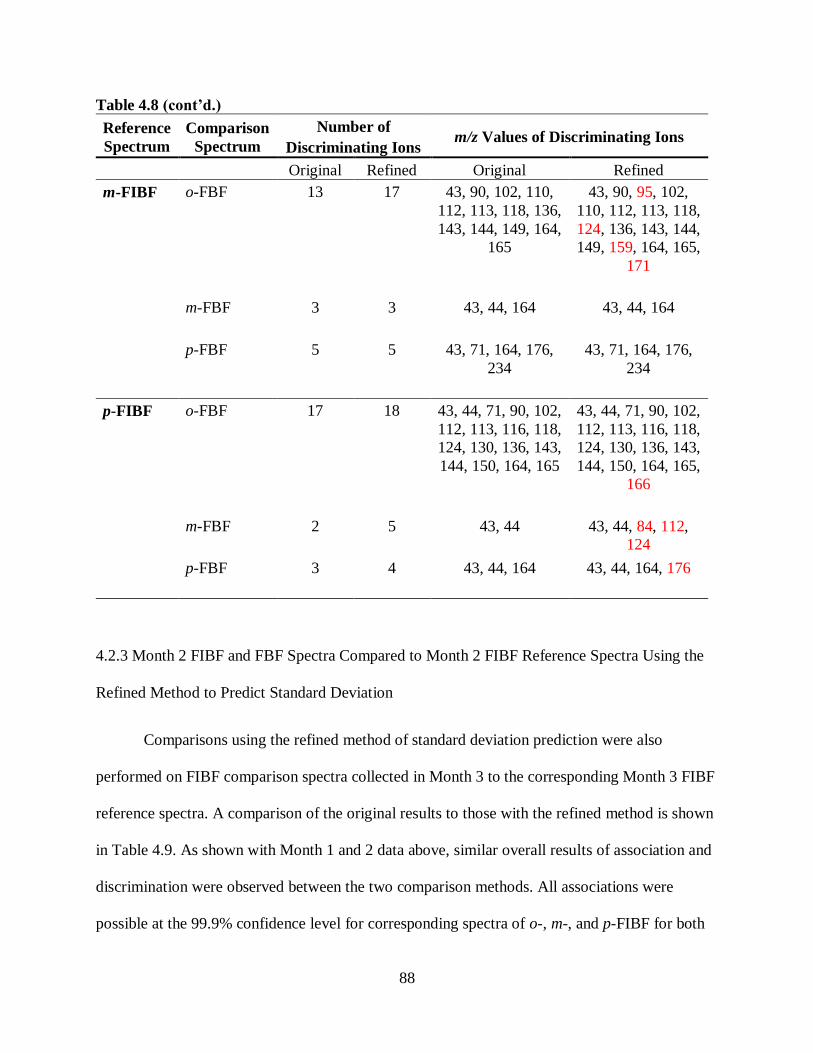
88


Reference

Spectrum

Comparison

Spectrum

Number of



m-FIBF o-FBF

13 17 43, 90, 102, 110,

112, 113, 118, 136,

143, 144, 149, 164,

165

43, 90, 95, 102,

110, 112, 113, 118,

124, 136, 143, 144,

149, 159, 164, 165,

171

m-FBF

3 3 43, 44, 164 43, 44, 164

p-FBF

5 5 43, 71, 164, 176,

234

43, 71, 164, 176,

234

p-FIBF o-FBF

17 18 43, 44, 71, 90, 102,

112, 113, 116, 118,

124, 130, 136, 143,

144, 150, 164, 165

43, 44, 71, 90, 102,

112, 113, 116, 118,

124, 130, 136, 143,

144, 150, 164, 165,

166

m-FBF

2 5 43, 44 43, 44, 84, 112,

124

p-FBF

3 4 43, 44, 164 43, 44, 164, 176



Comparisons using the refined method of standard deviation prediction were also

performed on FIBF comparison spectra collected in Month 3 to the corresponding Month 3 FIBF

reference spectra. A comparison of the original results to those with the refined method is shown

in Table 4.9. As shown with Month 1 and 2 data above, similar overall results of association and

discrimination were observed between the two comparison methods. All associations were

possible at the 99.9% confidence level for corresponding spectra of o-, m-, and p-FIBF for both

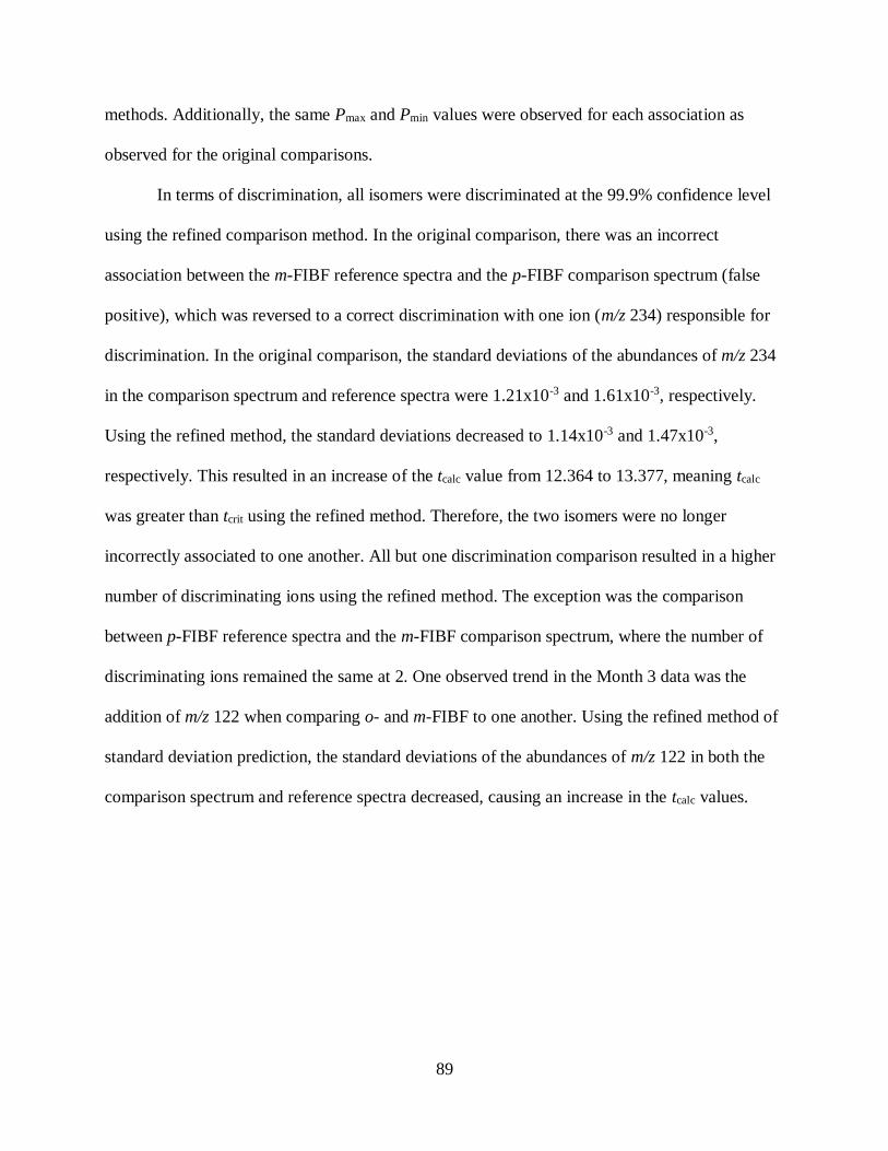
89

methods. Additionally, the same Pmax and Pmin values were observed for each association as

observed for the original comparisons.

In terms of discrimination, all isomers were discriminated at the 99.9% confidence level

using the refined comparison method. In the original comparison, there was an incorrect

association between the m-FIBF reference spectra and the p-FIBF comparison spectrum (false

positive), which was reversed to a correct discrimination with one ion (m/z 234) responsible for

discrimination. In the original comparison, the standard deviations of the abundances of m/z 234

in the comparison spectrum and reference spectra were 1.21x10-3 and 1.61x10-3, respectively.

Using the refined method, the standard deviations decreased to 1.14x10-3 and 1.47x10-3,

respectively. This resulted in an increase of the tcalc value from 12.364 to 13.377, meaning tcalc

was greater than tcrit using the refined method. Therefore, the two isomers were no longer

incorrectly associated to one another. All but one discrimination comparison resulted in a higher

number of discriminating ions using the refined method. The exception was the comparison

between p-FIBF reference spectra and the m-FIBF comparison spectrum, where the number of

discriminating ions remained the same at 2. One observed trend in the Month 3 data was the

addition of m/z 122 when comparing o- and m-FIBF to one another. Using the refined method of

standard deviation prediction, the standard deviations of the abundances of m/z 122 in both the

comparison spectrum and reference spectra decreased, causing an increase in the tcalc values.

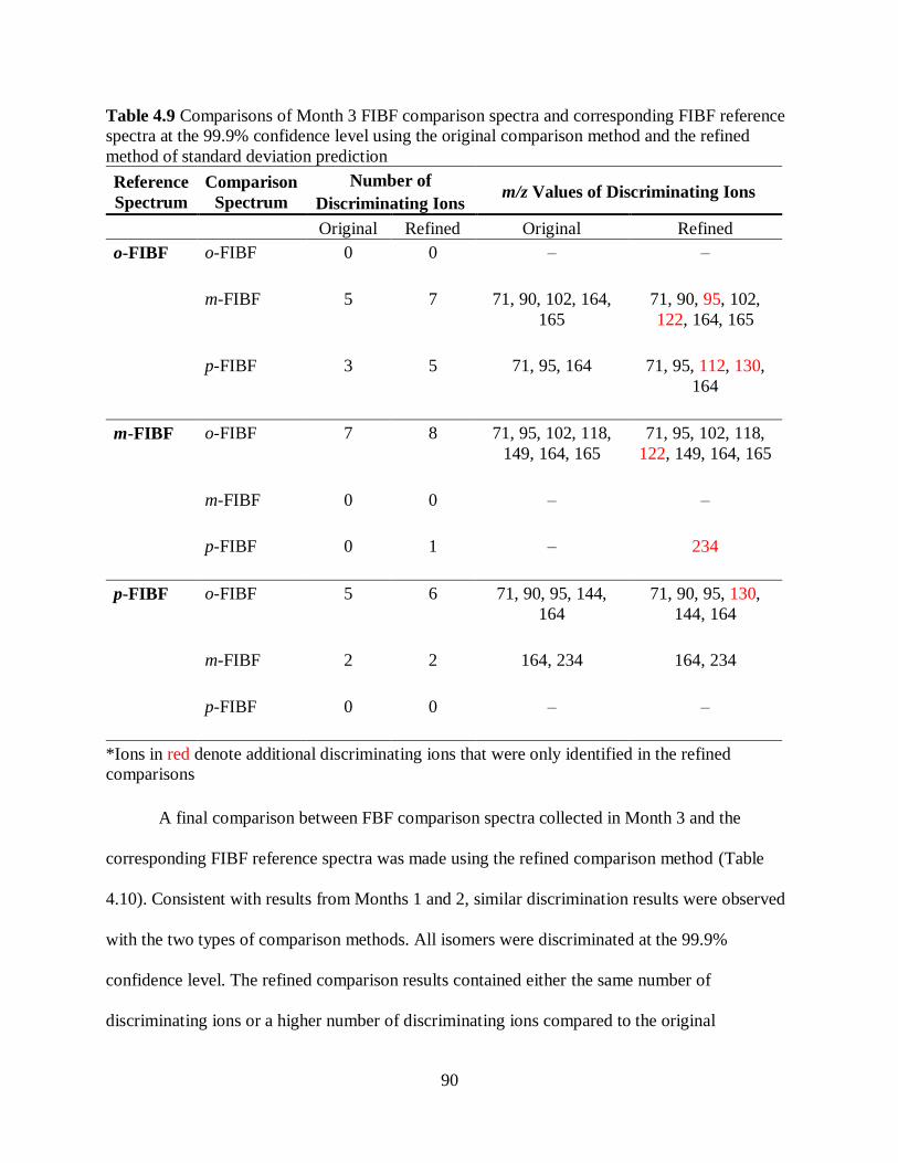
90




Reference

Spectrum

Comparison

Spectrum

Number of



o-FIBF o-FIBF

0 0 – –

m-FIBF 5 7 71, 90, 102, 164,

165

71, 90, 95, 102,

122, 164, 165

p-FIBF 3 5 71, 95, 164 71, 95, 112, 130,

164

m-FIBF o-FIBF 7 8 71, 95, 102, 118,

149, 164, 165

71, 95, 102, 118,

122, 149, 164, 165

m-FIBF

0 0 – –

p-FIBF 0 1 –

234

p-FIBF o-FIBF

5 6 71, 90, 95, 144,

164

71, 90, 95, 130,

144, 164

m-FIBF

2 2 164, 234 164, 234

p-FIBF

0 0 – –


comparisons

A final comparison between FBF comparison spectra collected in Month 3 and the

corresponding FIBF reference spectra was made using the refined comparison method (Table

4.10). Consistent with results from Months 1 and 2, similar discrimination results were observed

with the two types of comparison methods. All isomers were discriminated at the 99.9%

confidence level. The refined comparison results contained either the same number of

discriminating ions or a higher number of discriminating ions compared to the original

91

comparisons. Although no trends were observed in the identities of the additional discriminating

ions within the Month 3 data, only two ions m/z 102 and m/z 176 were observed in the FBF to

FIBF comparisons across all three months. For both ions, the tcalc values increased to greater than

the tcrit values of 12.924 for all months.




Reference

Spectrum

Comparison

Spectrum

Number of



o-FIBF o-FBF

2 2 43, 164 43, 164

m-FBF

8 9 43, 44, 71, 93, 95,

122, 148, 164

43, 44, 71, 90, 93,

95, 122, 148, 164

p-FBF 3 5 43, 44, 234 43, 44, 102, 176,

234

m-FIBF o-FBF

6 9 43, 90, 102, 118,

164, 165

43, 90, 102, 110,

118, 130, 149, 164,

165

m-FBF

4 4 43, 44, 93, 164 43, 44, 93, 164

p-FBF

3 5 43, 164, 234 43, 44, 164, 176,

234

p-FIBF o-FBF

14 14 43, 71, 90, 95, 102,

112, 118, 124, 130,

136, 143, 144, 164,

165

43, 71, 90, 95, 102,

112, 118, 124, 130,

136, 143, 144, 164,

165

m-FBF

2 3 43, 44 43, 44, 93

p-FBF

4 4 43, 44, 111, 164 43, 44, 111, 164


comparisons

92

4.4 Summary

Since the inter-month comparisons between Month 1 and Month 2 FIBF and FBF data

resulted in no correct association and discrimination with an unlikely number of ions responsible,

closer inspection of the regression lines was taken. While the regression plots were expected to

have a slope close to 0.5, where the standard deviation was proportional to abundance in a

manner similar to that expected for shot-noise limits, the slopes were approaching 1.0 instead.

These investigations resulted in testing the removal of outliers using a z-score test to determine

the effect on the ability to associate and discriminate the six isomers. No significant difference in

results was observed (Appendix Tables A4.1 – A4.12). Secondly, further investigation of the

regression data indicated that there may be two linear regions with two different slopes. The

breakpoint was determined manually and the resulting slopes and y-intercepts from the new

regression lines were input into a two-slope comparison version of the template and all

comparisons were re-evaluated.

For the Month 1 collections of FIBF and FBF comparison spectra, association and

discrimination were retained at the 99.9% confidence level. However, using the refined

comparison method resulted in an increase in the number of discriminating ions, with the largest

increase from 12 to 22 ions.

For the Month 2 collections, association and discrimination were also retained at the

99.9% confidence level. Once again, the use of the refined method to predict standard deviation

resulted in a higher number of discriminating ions for many of the comparisons than the use of

the original comparison method, with the largest increase being from 13 to 17 ions.

Finally, for the Month 3 collections, association was still possible using the refined

comparison method at the 99.9% confidence level. An incorrect association between m- and p-

93

FIBF using the original comparison method was corrected to a discrimination with one ion

responsible for discrimination (m/z 234) at the 99.9% confidence level. All other discriminations

were possible at the 99.9% confidence level using the refined method, and many of the

comparisons resulted in a higher number of discriminating ions.

Using the refined method to predict standard deviation resulted in similar overall

association and discrimination results of the comparisons of the two sets of isomers. However,

there was an increase in the number of discrimination ions in most comparisons as well as a

reversal of an incorrect association to a correct discrimination. These results may increase the

confidence in the discrimination power of the method and prove useful in a forensic laboratory

setting. In order to utilize the refined method to predict standard deviation based on two regions

of the regression, a more objective method of determining the breakpoint is necessary.

Alternatively, instead of using a method to predict standard deviation that involves using two

linear regions within a regression line, a more accurate equation which represents the additive

variation of all three sources of noise within the election multiplier response should be

investigated.

94

APPENDIX

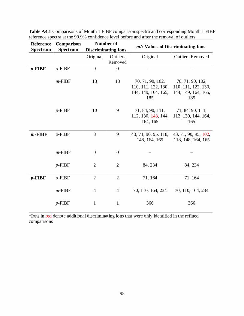
95


reference spectra at the 99.9% confidence level before and after the removal of outliers

Reference

Spectrum

Comparison

Spectrum

Number of


Original Outliers

Removed

Original Outliers Removed

o-FIBF o-FIBF

0 0 – –

m-FIBF 13 13 70, 71, 90, 102,

110, 111, 122, 130,

144, 149, 164, 165,

185

70, 71, 90, 102,

110, 111, 122, 130,

144, 149, 164, 165,

185

p-FIBF 10 9 71, 84, 90, 111,

112, 130, 143, 144,

164, 165

71, 84, 90, 111,

112, 130, 144, 164,

165

m-FIBF o-FIBF 8 9 43, 71, 90, 95, 118,

148, 164, 165

43, 71, 90, 95, 102,

118, 148, 164, 165

m-FIBF

0 0 – –

p-FIBF 2 2 84, 234 84, 234

p-FIBF o-FIBF

2 2 71, 164 71, 164

m-FIBF

4 4 70, 110, 164, 234

70, 110, 164, 234

p-FIBF

1 1 366 366


comparisons

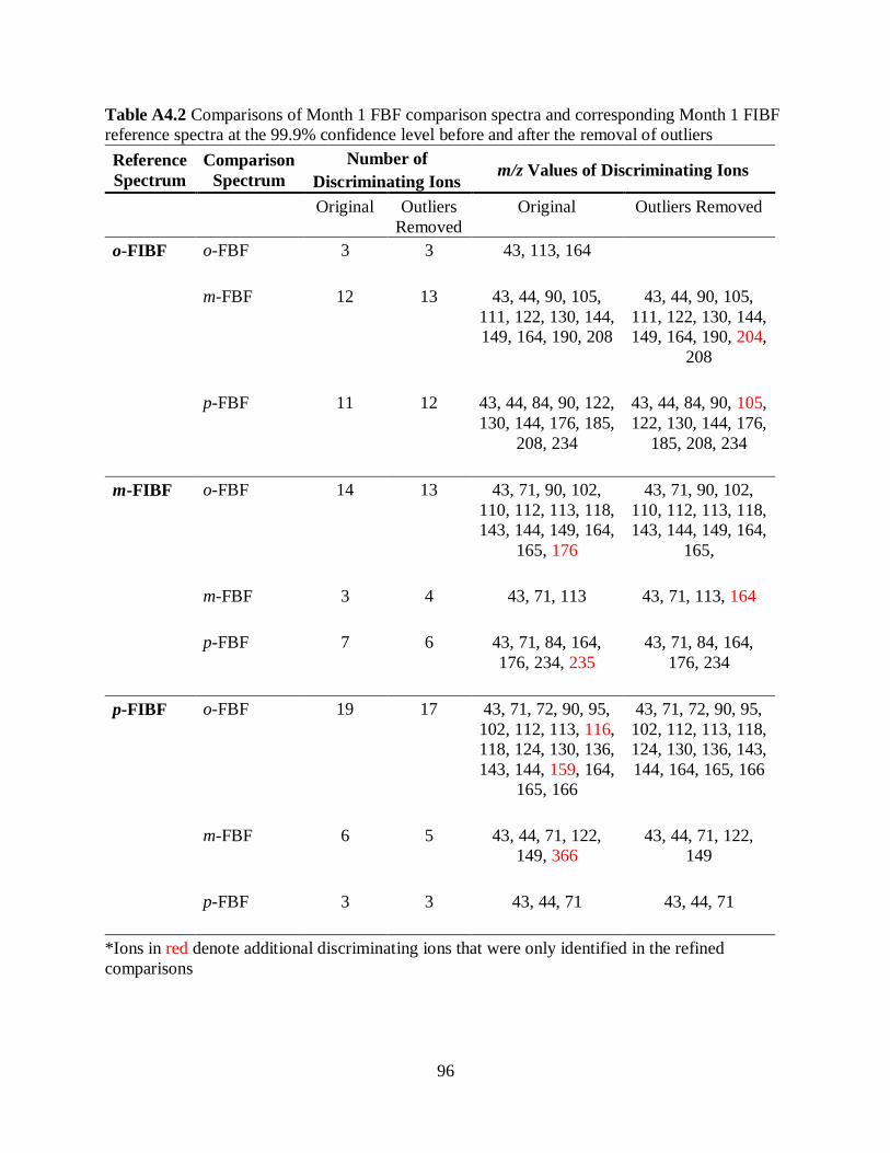
96



Reference

Spectrum

Comparison

Spectrum

Number of


Original Outliers

Removed


o-FIBF o-FBF

3 3 43, 113, 164

m-FBF

12 13 43, 44, 90, 105,

111, 122, 130, 144,

149, 164, 190, 208

43, 44, 90, 105,

111, 122, 130, 144,

149, 164, 190, 204,

208

p-FBF 11 12 43, 44, 84, 90, 122,

130, 144, 176, 185,

208, 234

43, 44, 84, 90, 105,

122, 130, 144, 176,

185, 208, 234

m-FIBF o-FBF

14 13 43, 71, 90, 102,

110, 112, 113, 118,

143, 144, 149, 164,

165, 176

43, 71, 90, 102,

110, 112, 113, 118,

143, 144, 149, 164,

165,

m-FBF

3 4 43, 71, 113 43, 71, 113, 164

p-FBF

7 6 43, 71, 84, 164,

176, 234, 235

43, 71, 84, 164,

176, 234

p-FIBF o-FBF

19 17 43, 71, 72, 90, 95,

102, 112, 113, 116,

118, 124, 130, 136,

143, 144, 159, 164,

165, 166

43, 71, 72, 90, 95,

102, 112, 113, 118,

124, 130, 136, 143,

144, 164, 165, 166

m-FBF

6 5 43, 44, 71, 122,

149, 366

43, 44, 71, 122,

149

p-FBF

3 3 43, 44, 71 43, 44, 71


comparisons

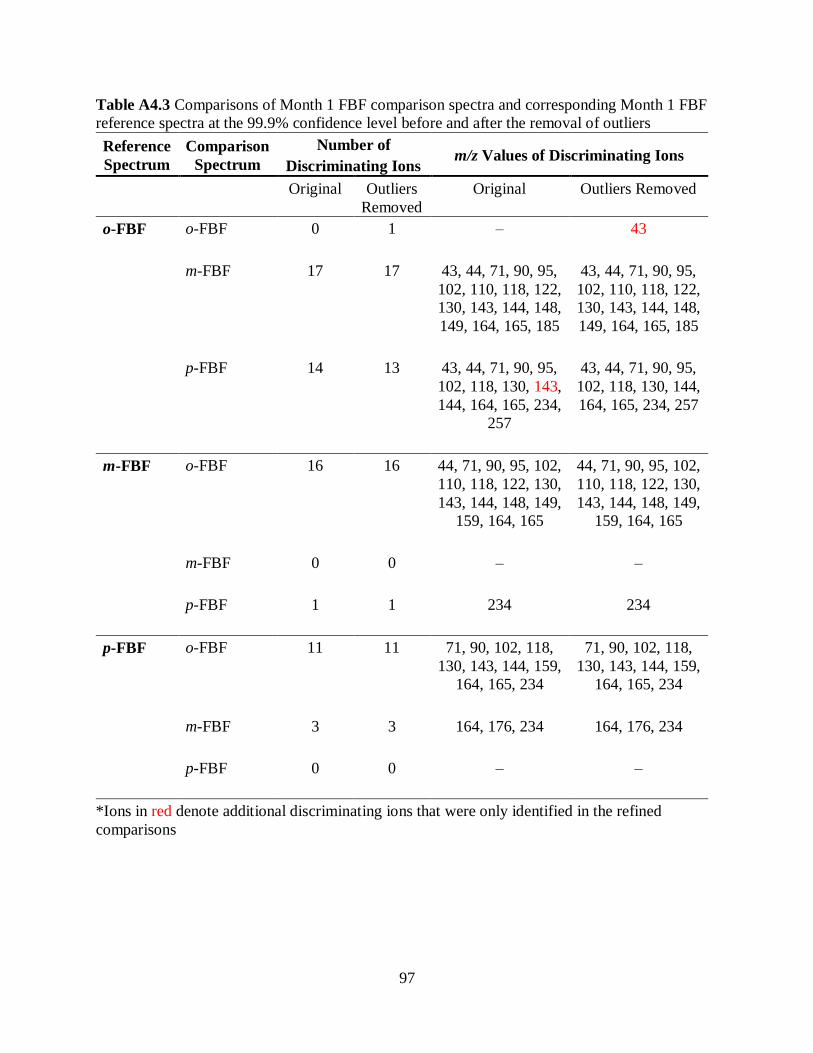
97



Reference

Spectrum

Comparison

Spectrum

Number of


Original Outliers

Removed


o-FBF o-FBF

0 1 – 43

m-FBF

17 17 43, 44, 71, 90, 95,

102, 110, 118, 122,

130, 143, 144, 148,

149, 164, 165, 185

43, 44, 71, 90, 95,

102, 110, 118, 122,

130, 143, 144, 148,

149, 164, 165, 185

p-FBF 14 13 43, 44, 71, 90, 95,

102, 118, 130, 143,

144, 164, 165, 234,

257

43, 44, 71, 90, 95,

102, 118, 130, 144,

164, 165, 234, 257

m-FBF o-FBF

16 16 44, 71, 90, 95, 102,

110, 118, 122, 130,

143, 144, 148, 149,

159, 164, 165

44, 71, 90, 95, 102,

110, 118, 122, 130,

143, 144, 148, 149,

159, 164, 165

m-FBF

0 0 – –

p-FBF

1 1 234 234

p-FBF o-FBF

11 11 71, 90, 102, 118,

130, 143, 144, 159,

164, 165, 234

71, 90, 102, 118,

130, 143, 144, 159,

164, 165, 234

m-FBF

3 3 164, 176, 234 164, 176, 234

p-FBF

0 0 – –


comparisons

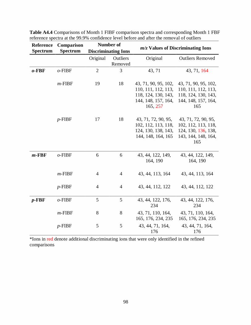
98



Reference

Spectrum

Comparison

Spectrum

Number of


Original Outliers

Removed


o-FBF o-FIBF

2 3 43, 71 43, 71, 164

m-FIBF 19 18 43, 71, 90, 95, 102,

110, 111, 112, 113,

118, 124, 130, 143,

144, 148, 157, 164,

165, 257

43, 71, 90, 95, 102,

110, 111, 112, 113,

118, 124, 130, 143,

144, 148, 157, 164,

165

p-FIBF 17 18 43, 71, 72, 90, 95,

102, 112, 113, 118,

124, 130, 138, 143,

144, 148, 164, 165

43, 71, 72, 90, 95,

102, 112, 113, 118,

124, 130, 136, 138,

143, 144, 148, 164,

165

m-FBF o-FIBF 6 6 43, 44, 122, 149,

164, 190

43, 44, 122, 149,

164, 190

m-FIBF

4 4 43, 44, 113, 164 43, 44, 113, 164

p-FIBF 4 4 43, 44, 112, 122 43, 44, 112, 122

p-FBF o-FIBF

5 5 43, 44, 122, 176,

234

43, 44, 122, 176,

234

m-FIBF

8 8 43, 71, 110, 164,

165, 176, 234, 235

43, 71, 110, 164,

165, 176, 234, 235

p-FIBF

5 5 43, 44, 71, 164,

176

43, 44, 71, 164,

176


comparisons

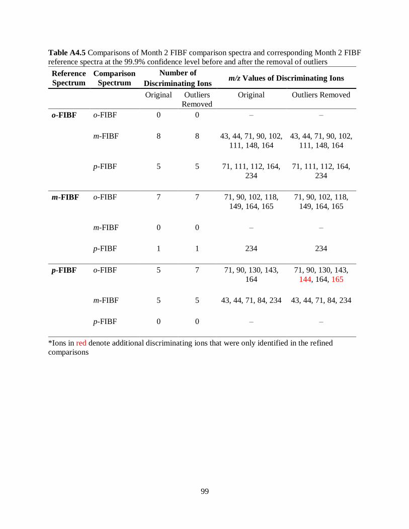
99



Reference

Spectrum

Comparison

Spectrum

Number of


Original Outliers

Removed


o-FIBF o-FIBF

0 0 – –

m-FIBF 8 8 43, 44, 71, 90, 102,

111, 148, 164

43, 44, 71, 90, 102,

111, 148, 164

p-FIBF 5 5 71, 111, 112, 164,

234

71, 111, 112, 164,

234

m-FIBF o-FIBF 7 7 71, 90, 102, 118,

149, 164, 165

71, 90, 102, 118,

149, 164, 165

m-FIBF

0 0 – –

p-FIBF 1 1 234

234

p-FIBF o-FIBF

5 7 71, 90, 130, 143,

164

71, 90, 130, 143,

144, 164, 165

m-FIBF

5 5 43, 44, 71, 84, 234 43, 44, 71, 84, 234

p-FIBF

0 0 – –


comparisons

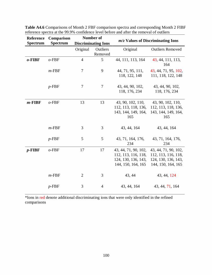
100



Reference

Spectrum

Comparison

Spectrum

Number of


Original Outliers

Removed


o-FIBF o-FBF

4 5 44, 111, 113, 164 43, 44, 111, 113,

164

m-FBF

7 9 44, 71, 95, 111,

118, 122, 148

43, 44, 71, 95, 102,

111, 118, 122, 148

p-FBF 7 7 43, 44, 90, 102,

118, 176, 234

43, 44, 90, 102,

118, 176, 234

m-FIBF o-FBF

13 13 43, 90, 102, 110,

112, 113, 118, 136,

143, 144, 149, 164,

165

43, 90, 102, 110,

112, 113, 118, 136,

143, 144, 149, 164,

165

m-FBF

3 3 43, 44, 164 43, 44, 164

p-FBF

5 5 43, 71, 164, 176,

234

43, 71, 164, 176,

234

p-FIBF o-FBF

17 17 43, 44, 71, 90, 102,

112, 113, 116, 118,

124, 130, 136, 143,

144, 150, 164, 165

43, 44, 71, 90, 102,

112, 113, 116, 118,

124, 130, 136, 143,

144, 150, 164, 165

m-FBF

2 3 43, 44 43, 44, 124

p-FBF

3 4 43, 44, 164 43, 44, 71, 164


comparisons

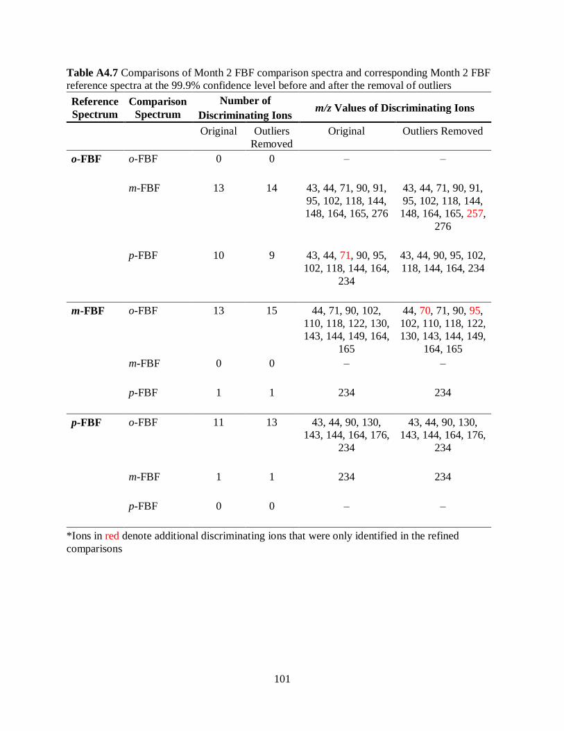
101



Reference

Spectrum

Comparison

Spectrum

Number of


Original Outliers

Removed


o-FBF o-FBF

0 0 – –

m-FBF

13 14 43, 44, 71, 90, 91,

95, 102, 118, 144,

148, 164, 165, 276

43, 44, 71, 90, 91,

95, 102, 118, 144,

148, 164, 165, 257,

276

p-FBF 10 9 43, 44, 71, 90, 95,

102, 118, 144, 164,

234

43, 44, 90, 95, 102,

118, 144, 164, 234

m-FBF o-FBF

13 15 44, 71, 90, 102,

110, 118, 122, 130,

143, 144, 149, 164,

165

44, 70, 71, 90, 95,

102, 110, 118, 122,

130, 143, 144, 149,

164, 165

m-FBF

0 0 – –

p-FBF

1 1 234 234

p-FBF o-FBF

11 13 43, 44, 90, 130,

143, 144, 164, 176,

234

43, 44, 90, 130,

143, 144, 164, 176,

234

m-FBF

1 1 234 234

p-FBF

0 0 – –


comparisons

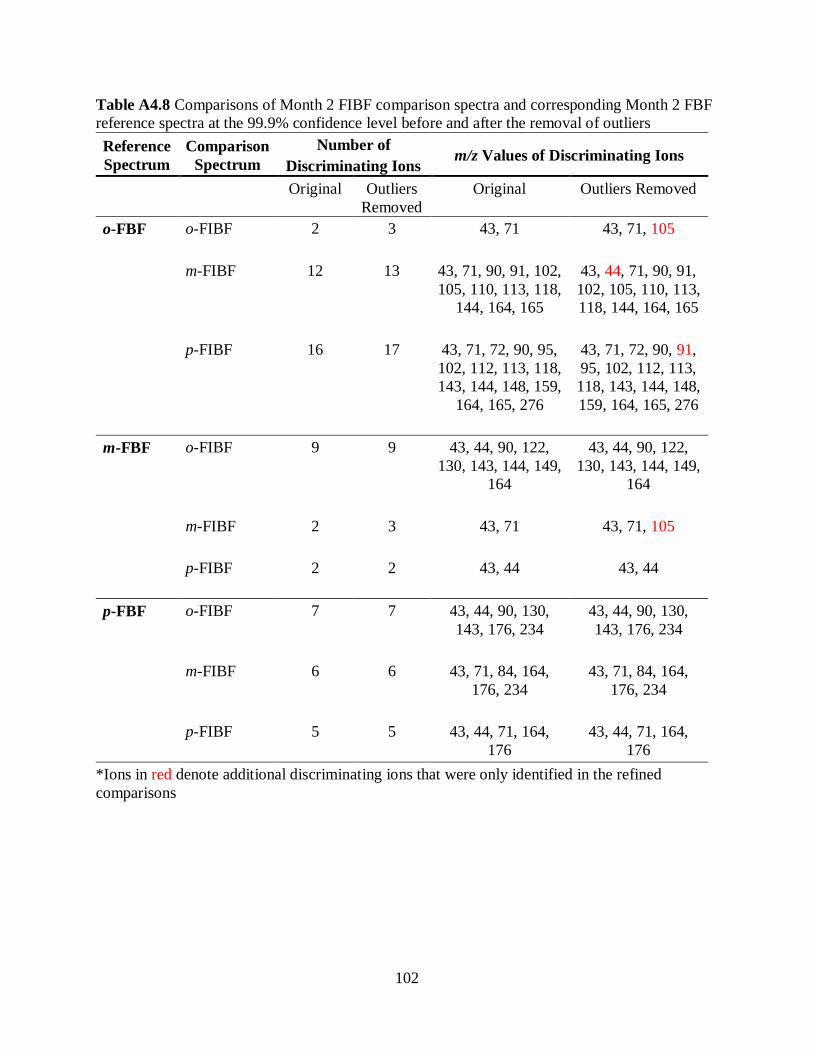
102



Reference

Spectrum

Comparison

Spectrum

Number of


Original Outliers

Removed


o-FBF o-FIBF

2 3 43, 71 43, 71, 105

m-FIBF 12 13 43, 71, 90, 91, 102,

105, 110, 113, 118,

144, 164, 165

43, 44, 71, 90, 91,

102, 105, 110, 113,

118, 144, 164, 165

p-FIBF 16 17 43, 71, 72, 90, 95,

102, 112, 113, 118,

143, 144, 148, 159,

164, 165, 276

43, 71, 72, 90, 91,

95, 102, 112, 113,

118, 143, 144, 148,

159, 164, 165, 276

m-FBF o-FIBF 9 9 43, 44, 90, 122,

130, 143, 144, 149,

164

43, 44, 90, 122,

130, 143, 144, 149,

164

m-FIBF

2 3 43, 71 43, 71, 105

p-FIBF 2 2 43, 44 43, 44

p-FBF o-FIBF

7 7 43, 44, 90, 130,

143, 176, 234

43, 44, 90, 130,

143, 176, 234

m-FIBF

6 6 43, 71, 84, 164,

176, 234

43, 71, 84, 164,

176, 234

p-FIBF

5 5 43, 44, 71, 164,

176

43, 44, 71, 164,

176


comparisons

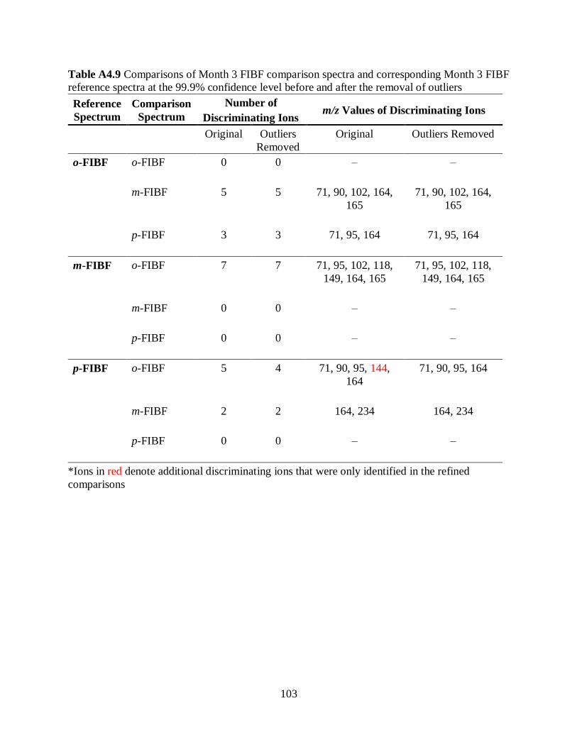
103



Reference

Spectrum

Comparison

Spectrum

Number of


Original Outliers

Removed


o-FIBF o-FIBF

0 0 – –

m-FIBF 5 5 71, 90, 102, 164,

165

71, 90, 102, 164,

165

p-FIBF 3 3 71, 95, 164 71, 95, 164

m-FIBF o-FIBF 7 7 71, 95, 102, 118,

149, 164, 165

71, 95, 102, 118,

149, 164, 165

m-FIBF

0 0 – –

p-FIBF 0 0 –

–

p-FIBF o-FIBF

5 4 71, 90, 95, 144,

164

71, 90, 95, 164

m-FIBF

2 2 164, 234 164, 234

p-FIBF

0 0 – –


comparisons

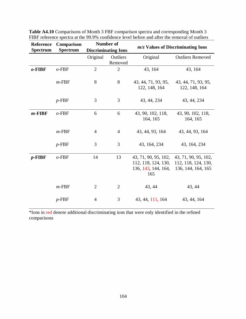
104

Table A4.10 Comparisons of Month 3 FBF comparison spectra and corresponding Month 3

FIBF reference spectra at the 99.9% confidence level before and after the removal of outliers

Reference

Spectrum

Comparison

Spectrum

Number of


Original Outliers

Removed


o-FIBF o-FBF

2 2 43, 164 43, 164

m-FBF

8 8 43, 44, 71, 93, 95,

122, 148, 164

43, 44, 71, 93, 95,

122, 148, 164

p-FBF 3 3 43, 44, 234 43, 44, 234

m-FIBF o-FBF

6 6 43, 90, 102, 118,

164, 165

43, 90, 102, 118,

164, 165

m-FBF

4 4 43, 44, 93, 164 43, 44, 93, 164

p-FBF

3 3 43, 164, 234 43, 164, 234

p-FIBF o-FBF

14 13 43, 71, 90, 95, 102,

112, 118, 124, 130,

136, 143, 144, 164,

165

43, 71, 90, 95, 102,

112, 118, 124, 130,

136, 144, 164, 165

m-FBF

2 2 43, 44 43, 44

p-FBF

4 3 43, 44, 111, 164 43, 44, 164


comparisons

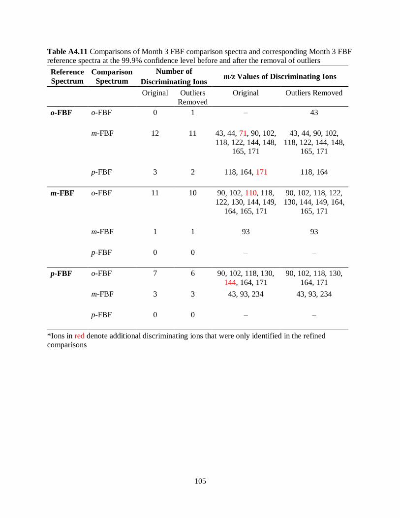
105



Reference

Spectrum

Comparison

Spectrum

Number of


Original Outliers

Removed


o-FBF o-FBF

0 1 – 43

m-FBF

12 11 43, 44, 71, 90, 102,

118, 122, 144, 148,

165, 171

43, 44, 90, 102,

118, 122, 144, 148,

165, 171

p-FBF 3 2 118, 164, 171 118, 164

m-FBF o-FBF

11 10 90, 102, 110, 118,

122, 130, 144, 149,

164, 165, 171

90, 102, 118, 122,

130, 144, 149, 164,

165, 171

m-FBF

1 1 93 93

p-FBF

0 0 – –

p-FBF o-FBF

7 6 90, 102, 118, 130,

144, 164, 171

90, 102, 118, 130,

164, 171

m-FBF

3 3 43, 93, 234 43, 93, 234

p-FBF

0 0 – –


comparisons

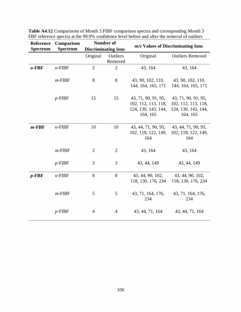
106

Table A4.12 Comparisons of Month 3 FIBF comparison spectra and corresponding Month 3

FBF reference spectra at the 99.9% confidence level before and after the removal of outliers

Reference

Spectrum

Comparison

Spectrum

Number of


Original Outliers

Removed


o-FBF o-FIBF

2 2 43, 164 43, 164

m-FIBF 8 8 43, 90, 102, 110,

144, 164, 165, 171

43, 90, 102, 110,

144, 164, 165, 171

p-FIBF 15 15 43, 71, 90, 91, 95,

102, 112, 113, 118,

124, 130, 143, 144,

164, 165

43, 71, 90, 91, 95,

102, 112, 113, 118,

124, 130, 143, 144,

164, 165

m-FBF o-FIBF 10 10 43, 44, 71, 90, 95,

102, 118, 122, 149,

164

43, 44, 71, 90, 95,

102, 118, 122, 149,

164

m-FIBF

2 2 43, 164 43, 164

p-FIBF 3 3 43, 44, 149

43, 44, 149

p-FBF o-FIBF

8 8 43, 44, 90, 102,

118, 130, 176, 234

43, 44, 90, 102,

118, 130, 176, 234

m-FIBF

5 5 43, 71, 164, 176,

234

43, 71, 164, 176,

234

p-FIBF

4 4 43, 44, 71, 164 43, 44, 71, 164

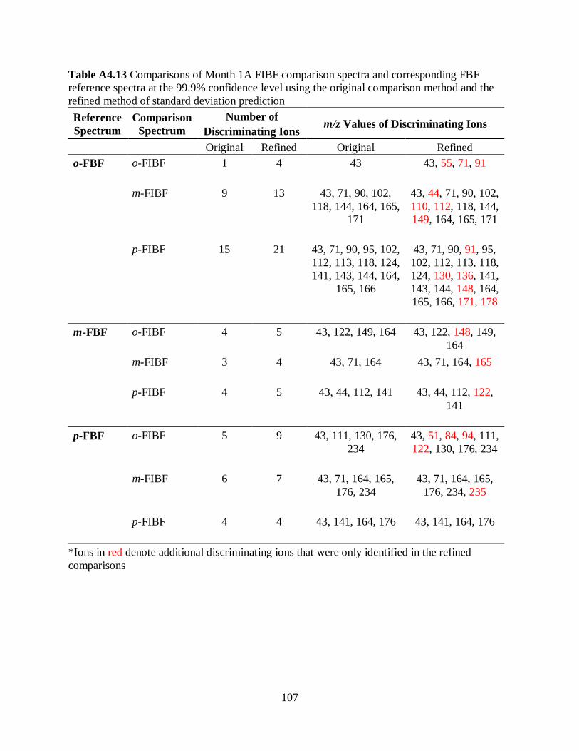
107

Table A4.13 Comparisons of Month 1A FIBF comparison spectra and corresponding FBF



Reference

Spectrum

Comparison

Spectrum

Number of



o-FBF o-FIBF

1 4 43 43, 55, 71, 91

m-FIBF 9

13 43, 71, 90, 102,

118, 144, 164, 165,

171

43, 44, 71, 90, 102,

110, 112, 118, 144,

149, 164, 165, 171

p-FIBF 15 21 43, 71, 90, 95, 102,

112, 113, 118, 124,

141, 143, 144, 164,

165, 166

43, 71, 90, 91, 95,

102, 112, 113, 118,

124, 130, 136, 141,

143, 144, 148, 164,

165, 166, 171, 178

m-FBF o-FIBF 4

5 43, 122, 149, 164 43, 122, 148, 149,

164

m-FIBF

3 4 43, 71, 164 43, 71, 164, 165

p-FIBF 4 5 43, 44, 112, 141 43, 44, 112, 122,

141

p-FBF o-FIBF

5 9 43, 111, 130, 176,

234

43, 51, 84, 94, 111,

122, 130, 176, 234

m-FIBF

6 7 43, 71, 164, 165,

176, 234

43, 71, 164, 165,

176, 234, 235

p-FIBF

4 4 43, 141, 164, 176 43, 141, 164, 176


comparisons

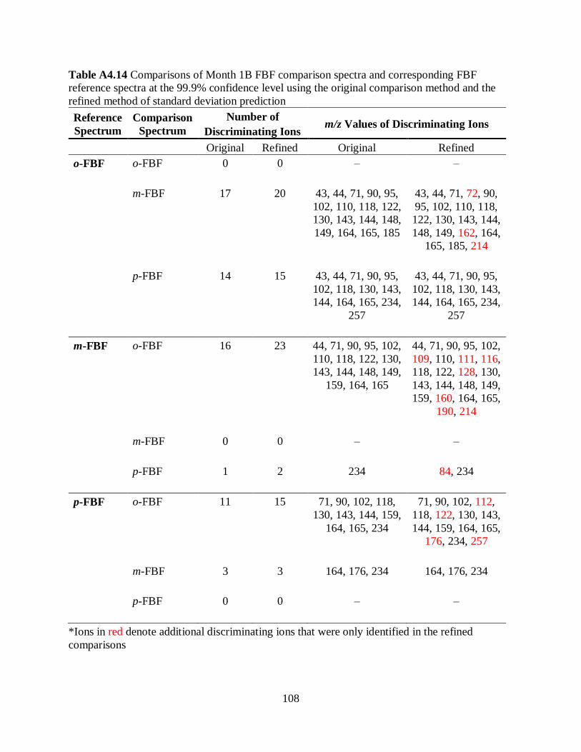
108

Table A4.14 Comparisons of Month 1B FBF comparison spectra and corresponding FBF



Reference

Spectrum

Comparison

Spectrum

Number of



o-FBF o-FBF

0 0 – –

m-FBF

17 20 43, 44, 71, 90, 95,

102, 110, 118, 122,

130, 143, 144, 148,

149, 164, 165, 185

43, 44, 71, 72, 90,

95, 102, 110, 118,

122, 130, 143, 144,

148, 149, 162, 164,

165, 185, 214

p-FBF 14 15 43, 44, 71, 90, 95,

102, 118, 130, 143,

144, 164, 165, 234,

257

43, 44, 71, 90, 95,

102, 118, 130, 143,

144, 164, 165, 234,

257

m-FBF o-FBF

16 23 44, 71, 90, 95, 102,

110, 118, 122, 130,

143, 144, 148, 149,

159, 164, 165

44, 71, 90, 95, 102,

109, 110, 111, 116,

118, 122, 128, 130,

143, 144, 148, 149,

159, 160, 164, 165,

190, 214

m-FBF

0 0 – –

p-FBF 1 2 234 84, 234

p-FBF o-FBF

11 15 71, 90, 102, 118,

130, 143, 144, 159,

164, 165, 234

71, 90, 102, 112,

118, 122, 130, 143,

144, 159, 164, 165,

176, 234, 257

m-FBF

3 3 164, 176, 234 164, 176, 234

p-FBF 0 0 – –


comparisons

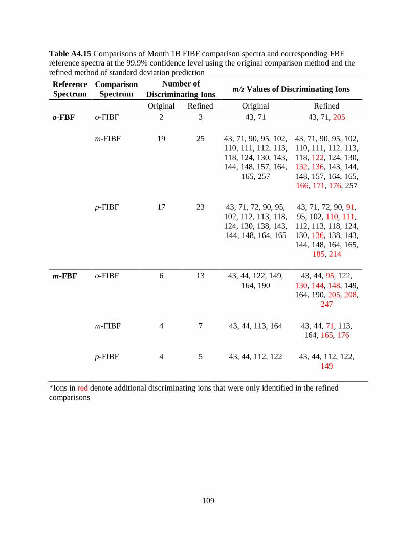
109

Table A4.15 Comparisons of Month 1B FIBF comparison spectra and corresponding FBF



Reference

Spectrum

Comparison

Spectrum

Number of



o-FBF o-FIBF

2 3 43, 71 43, 71, 205

m-FIBF 19 25 43, 71, 90, 95, 102,

110, 111, 112, 113,

118, 124, 130, 143,

144, 148, 157, 164,

165, 257

43, 71, 90, 95, 102,

110, 111, 112, 113,

118, 122, 124, 130,

132, 136, 143, 144,

148, 157, 164, 165,

166, 171, 176, 257

p-FIBF 17 23 43, 71, 72, 90, 95,

102, 112, 113, 118,

124, 130, 138, 143,

144, 148, 164, 165

43, 71, 72, 90, 91,

95, 102, 110, 111,

112, 113, 118, 124,

130, 136, 138, 143,

144, 148, 164, 165,

185, 214

m-FBF o-FIBF 6 13 43, 44, 122, 149,

164, 190

43, 44, 95, 122,

130, 144, 148, 149,

164, 190, 205, 208,

247

m-FIBF

4 7 43, 44, 113, 164 43, 44, 71, 113,

164, 165, 176

p-FIBF 4 5 43, 44, 112, 122 43, 44, 112, 122,

149


comparisons

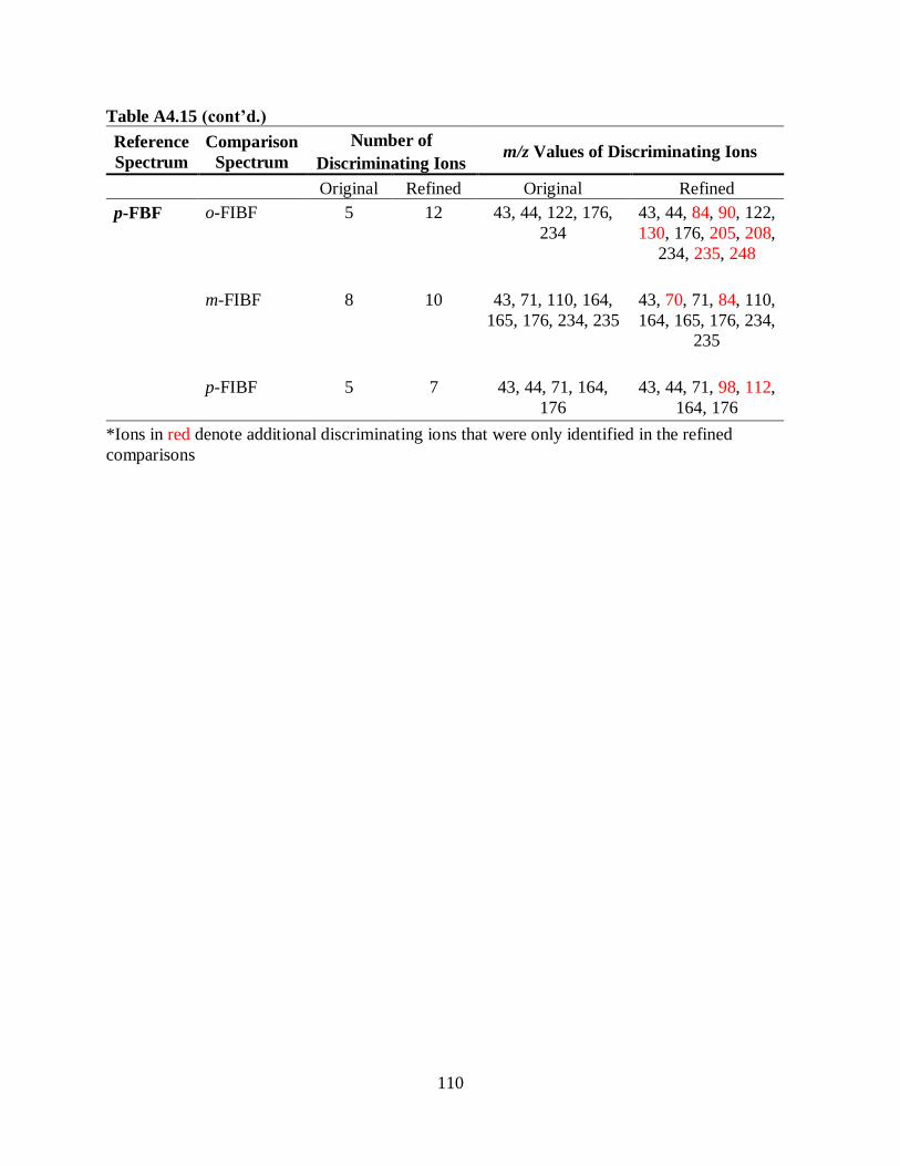
110

Table A4.15 (cont’d.)

Reference

Spectrum

Comparison

Spectrum

Number of



p-FBF o-FIBF

5 12 43, 44, 122, 176,

234

43, 44, 84, 90, 122,

130, 176, 205, 208,

234, 235, 248

m-FIBF

8 10 43, 71, 110, 164,

165, 176, 234, 235

43, 70, 71, 84, 110,

164, 165, 176, 234,

235

p-FIBF

5 7 43, 44, 71, 164,

176

43, 44, 71, 98, 112,

164, 176


comparisons

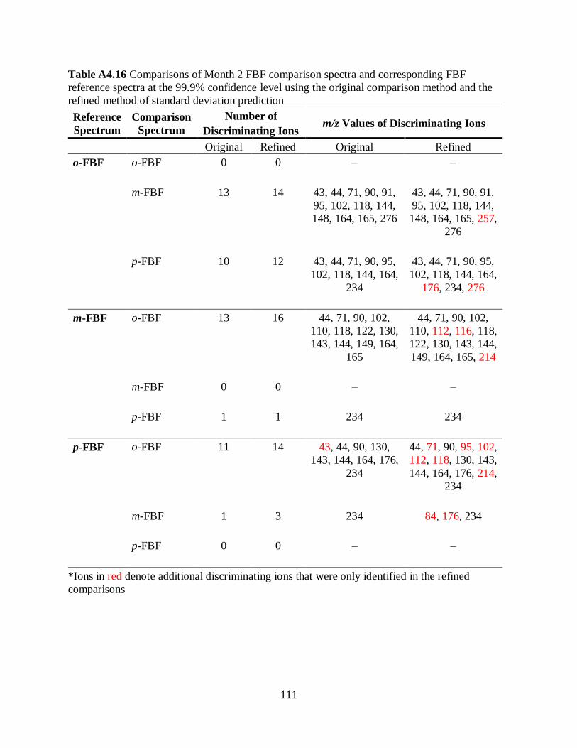
111




Reference

Spectrum

Comparison

Spectrum

Number of



o-FBF o-FBF

0 0 – –

m-FBF

13 14 43, 44, 71, 90, 91,

95, 102, 118, 144,

148, 164, 165, 276

43, 44, 71, 90, 91,

95, 102, 118, 144,

148, 164, 165, 257,

276

p-FBF 10 12 43, 44, 71, 90, 95,

102, 118, 144, 164,

234

43, 44, 71, 90, 95,

102, 118, 144, 164,

176, 234, 276

m-FBF o-FBF

13 16 44, 71, 90, 102,

110, 118, 122, 130,

143, 144, 149, 164,

165

44, 71, 90, 102,

110, 112, 116, 118,

122, 130, 143, 144,

149, 164, 165, 214

m-FBF

0 0 – –

p-FBF

1 1 234 234

p-FBF o-FBF

11 14 43, 44, 90, 130,

143, 144, 164, 176,

234

44, 71, 90, 95, 102,

112, 118, 130, 143,

144, 164, 176, 214,

234

m-FBF

1 3 234 84, 176, 234

p-FBF

0 0 – –


comparisons

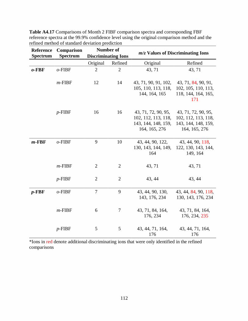
112




Reference

Spectrum

Comparison

Spectrum

Number of



o-FBF o-FIBF

2 2 43, 71 43, 71

m-FIBF 12 14 43, 71, 90, 91, 102,

105, 110, 113, 118,

144, 164, 165

43, 71, 84, 90, 91,

102, 105, 110, 113,

118, 144, 164, 165,

171

p-FIBF 16 16 43, 71, 72, 90, 95,

102, 112, 113, 118,

143, 144, 148, 159,

164, 165, 276

43, 71, 72, 90, 95,

102, 112, 113, 118,

143, 144, 148, 159,

164, 165, 276

m-FBF o-FIBF 9 10 43, 44, 90, 122,

130, 143, 144, 149,

164

43, 44, 90, 118,

122, 130, 143, 144,

149, 164

m-FIBF

2 2 43, 71 43, 71

p-FIBF 2 2 43, 44 43, 44

p-FBF o-FIBF

7 9 43, 44, 90, 130,

143, 176, 234

43, 44, 84, 90, 118,

130, 143, 176, 234

m-FIBF

6 7 43, 71, 84, 164,

176, 234

43, 71, 84, 164,

176, 234, 235

p-FIBF

5 5 43, 44, 71, 164,

176

43, 44, 71, 164,

176


comparisons

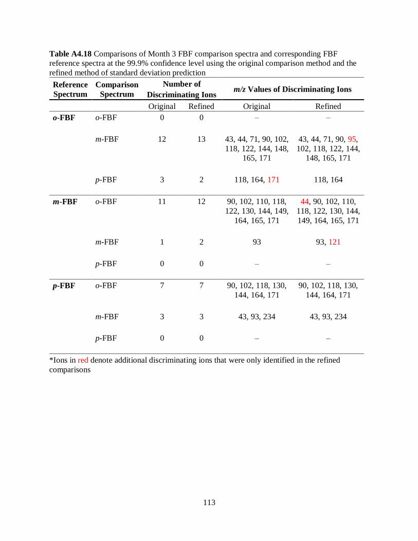
113




Reference

Spectrum

Comparison

Spectrum

Number of



o-FBF o-FBF

0 0 – –

m-FBF

12 13 43, 44, 71, 90, 102,

118, 122, 144, 148,

165, 171

43, 44, 71, 90, 95,

102, 118, 122, 144,

148, 165, 171

p-FBF 3 2 118, 164, 171 118, 164

m-FBF o-FBF

11 12 90, 102, 110, 118,

122, 130, 144, 149,

164, 165, 171

44, 90, 102, 110,

118, 122, 130, 144,

149, 164, 165, 171

m-FBF

1 2 93 93, 121

p-FBF

0 0 – –

p-FBF o-FBF

7 7 90, 102, 118, 130,

144, 164, 171

90, 102, 118, 130,

144, 164, 171

m-FBF

3 3 43, 93, 234 43, 93, 234

p-FBF

0 0 – –


comparisons

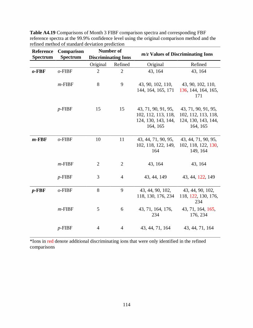
114




Reference

Spectrum

Comparison

Spectrum

Number of



o-FBF o-FIBF

2 2 43, 164 43, 164

m-FIBF 8 9 43, 90, 102, 110,

144, 164, 165, 171

43, 90, 102, 110,

136, 144, 164, 165,

171

p-FIBF 15 15 43, 71, 90, 91, 95,

102, 112, 113, 118,

124, 130, 143, 144,

164, 165

43, 71, 90, 91, 95,

102, 112, 113, 118,

124, 130, 143, 144,

164, 165

m-FBF o-FIBF 10 11 43, 44, 71, 90, 95,

102, 118, 122, 149,

164

43, 44, 71, 90, 95,

102, 118, 122, 130,

149, 164

m-FIBF

2 2 43, 164 43, 164

p-FIBF 3 4 43, 44, 149 43, 44, 122, 149

p-FBF o-FIBF

8 9 43, 44, 90, 102,

118, 130, 176, 234

43, 44, 90, 102,

118, 122, 130, 176,

234

m-FIBF

5 6 43, 71, 164, 176,

234

43, 71, 164, 165,

176, 234

p-FIBF

4 4 43, 44, 71, 164 43, 44, 71, 164


comparisons

115

REFERENCES

116

REFERENCES

(1) Detection of Outliers. NIST/SEMATECH e-Handbook of Statistical Methods. Section 3.

https://doi.org/10.18434/M32189

(2) Oosterbaan, R. J. Frequency and Regression Analysis of Hydrologic Data Part II: Regression

Analysis. Drainage Principles and Applications, 2nd ed, International Institute for Land

Reclamation and Improvement, 1994, Chapter 6.

https://doi.org/10.18434/M32189

117

V. Conclusions and Future Work

5.1 Conclusions

The overall objective in this research was to investigate the robustness of the previously

developed statistical comparison method to differentiate positional isomers using mass spectral

data. Mass spectra of two sets of fentanyl isomers, fluoroisobutyryl fentanyl (FIBF) and

fluorobutyryl fentanyl (FBF), collected during a three-month period, were used in this work.

First, association and discrimination of the isomers within and between each set was investigated

with mass spectra collected in the first month of analysis. Spectra of the FIBF positional isomers

and the FIBF and FBF structural isomers were correctly associated and discriminated, mostly at

the 99.9% confidence level, with only three exceptions. During the three-month study, the effects

of major instrument maintenance (involving venting of the system) as well as high instrument

usage (involving other research groups using the same instrument for a multitude of purposes) on

the ability to maintain proper association and discrimination of the fentanyl isomers were

investigated. Throughout the three months, the overall success of appropriate association and

discrimination was maintained at the 99.9% confidence level, with small differences in the

number and m/z value of discriminating ions. Nonetheless, certain ions were identified as reliable

ions for the discrimination between the positional isomers of FIBF and the structural isomers of

FIBF and FBF.

In addition, the method used to predict standard deviation based on modeling the electron

multiplier response was further refined by testing the effects of removing outliers and using two-

slopes to better describe the data. While removing outliers had a negligible effect on the

outcomes of the statistical comparisons, the investigation into using two separate slopes to more

118

accurately model the electron multiplier response proved to positively impact the statistical

comparisons. One incorrect association (false positive) was reversed to a discrimination and

many of the discriminating comparisons resulted in a greater number of discriminating ions,

giving more confidence in the distinction of the fentanyl isomers.

This user-friendly and rapid statistical comparison method can be implemented into

forensic laboratories to analyze submitted samples using mass spectral data that are already

routinely collected. Typically, a forensic analyst will analyze a submitted sample using gas

chromatography-mass spectrometry (GC-MS) and compare the resulting mass spectrum to a

spectral library within the analysis software. Using the initial identification from the mass

spectral library, a reference standard can be analyzed, and the data can be visually compared. In

additional to the visual comparison, the mass spectra of the submitted sample and that of the

reference standard could be entered into the statistical comparison method to determine if the

two spectra are statistically distinguishable or indistinguishable from one another. Using this

method, in addition to a visual assessment of the spectra, allows for statistical confidence in the

identification of the submitted sample. And, in cases where the two spectra are statistically

different, the ions responsible for identification can be identified.

5.2 Future Work

This work focused on demonstrating the ability of the statistical comparison method to

discriminate two sets of fentanyl isomers: FIBF and FBF positional isomers. The method has

also been applied to successfully discriminate positional isomers of ethylmethcathinone (EMC)

and fluoromethamphetamine (FMA).1 Given the increase in submissions of novel psychoactive

substances (NPS) and related isomers in forensic laboratories, further investigation into the

robustness of the method is warranted. Fentanyl and NPS analogs are a growing problem in the

119

United States and are expected to remain a serious threat in the years to come.2 Therefore, the

ability to identify a wide range of positional isomers using instrumentation that is readily

available in laboratories would be an advantage. In order to obtain that statistical confidence, the

statistical comparison method must be tested on a wide range of NPS analogs.

In order to truly refine the method of standard deviation prediction, a new method to

model the electron multiplier response should be investigated. Instead of automating a method to

separate the regression line into two linear regions, using a curve to represent the three sources of

noise (background, shot, and proportional) would be more accurate and potentially lead to more

accurate comparison results.

Additionally, a true concentration study should be performed to determine the ability of

the statistical comparison method to discriminate isomers at various concentrations. Previous

research indicates that lower concentration of sample results in fewer discriminating ions

present; therefore, a full concentration study would allow the determination of optimal

concentrations to be used for statistical comparisons. A more in depth concentration study would

also allow the determination of concentrations below the threshold for accurate association and

discrimination.1

Finally, the statistical comparison method should be applied to blind samples and case

work samples to further evaluate the robustness and ruggedness of the method. This test would

be a true determination of how successfully the statistical comparison method could be applied to

forensic case work.

Through these additional studies, as well as further refinement of the method of standard

deviation, continued evaluation of the robustness of the statistical comparison method is

possible. While these steps are needed, this work has demonstrated the ability of the method to

120

successfully discriminate between two sets of structural and positional isomers with a high

degree of spectral similarity. By testing the method on fentanyl isomers, the method was applied

to a new range of NPS compounds that have proven to be difficult to discriminate using other

methods. Additionally, the preliminary study into the effects of refining the method of standard

deviation prediction on the association and discrimination demonstrated the potential

effectiveness of utilizing a segmented regression analysis to increase the statistical confidence in

discriminating power.

121

REFERENCES

122

REFERENCES

(1) Stuhmer, Emma. Statistical Comparison of Mass Spectral Data for Positional Isomer

Differentiation, [Internet]. 2019; Available from: https://d.lib.msu.edu/etd/48160

(2) Drug Enforcement Administration. National Drug Threat Assessment; Washington, D.C.:

U.S. Department of Justice, Drug Enforcement Administration, 2019.

(3) Oosterbaan, R. J.; Sharma, D. P.; Singh, K. N.; Rao, K. V. G. K. Crop production and soil

salinity: Evaluation of field data from India by segmented linear regression with breakpoint.

Proceedings of the Symposium on Land Drainage for Salinity Control in Arid and Semi-Arid

Regions. 1990, Vol 3 Session V, 373-383.

https://d.lib.msu.edu/etd/48160

Documents

INVESTIGATING THE ROBUSTNESS OF A STATISTICAL METHOD …