Embed Size (px)
Citation preview
Robust Standard Errors in Small Samples: Some Practical Advice∗
Guido W. Imbens† Michal Kolesar‡
First Draft: October 2012
This Draft: March 2016
Abstract
We study the properties of heteroscedasticity-robust confidence intervals for regres-
sion parameters. We show that confidence intervals based on a degrees-of-freedom
correction suggested by Bell and McCaffrey [2002] are a natural extension of a prin-
cipled approach to the Behrens-Fisher problem. We suggest a further improvement
for the case with clustering. We show that these standard errors can lead to sub-
stantial improvements in coverage rates even for samples with fifty or more clusters.
We recommend researchers routinely calculate the Bell-McCaffrey degrees-of-freedom
adjustment to assess potential problems with conventional robust standard errors.
JEL Classification: C14, C21, C52
Keywords: Behrens-Fisher Problem, Robust Standard Errors, Small Samples,
Clustering
∗ Financial support for this research was generously provided through NSF grant 0820361.† Graduate School of Business, Stanford University, and NBER. Electronic correspon-
dence: [email protected].‡ Department of Economics and Woodrow Wilson School, Princeton University. Electronic
correspondence: [email protected].
[1]

1 Introduction
It is currently common practice in empirical work to use standard errors and associated
confidence intervals that are robust to the presence of heteroskedasticity. The most widely
used form of the robust, heteroskedasticity-consistent standard errors is that associated with
the work of White [1980] (see also Eicker [1967], Huber [1967]), extended to the case with
clustering by Liang and Zeger [1986]. The justification for these standard errors and the
associated confidence intervals is asymptotic: they rely on large samples for their validity.
In small samples the properties of these procedures are not always attractive: the robust
(Eicker-Huber-White, or EHW, and Liang-Zeger or LZ, from hereon) variance estimators
are biased downward, and the Normal-distribution-based confidence intervals using these
variance estimators can have coverage substantially below nominal coverage rates.
There is a large theoretical literature documenting and addressing these small sample
problems in the context of linear regression models, some of it reviewed in MacKinnon and
White [1985], Angrist and Pischke [2009, Chapter 8], and MacKinnon [2012]. A number
of alternative versions of the robust variance estimators and confidence intervals have been
proposed to deal with these problems. Some of these alternatives focus on reducing the
bias of the variance estimators [MacKinnon and White, 1985], some exploit higher order
expansions [Hausman and Palmer, 2011], others attempt to improve their properties by
using resampling methods [Davidson and Flachaire, 2008, Cameron et al., 2008, Hausman and
Palmer, 2011], or data-partitioning [Ibragimov and Muller, 2010], and some use t-distribution
approximations [Bell and McCaffrey, 2002, Donald and Lang, 2007]. Given the multitude of
alternatives, combined with the ad hoc nature of some of them, it is not clear, however, how
to choose among them. Moreover, some researchers [e.g. Angrist and Pischke, 2009, Chapter
8.2.3] argue that for commonly encountered sample sizes—fifty or more units / fifty or more
clusters—using these alternatives is not necessary because the EHW and LZ standard errors
perform well.
We make three specific points in this paper. First, we show that a particular improvement
[2]
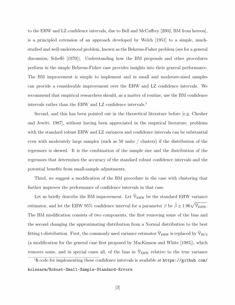
to the EHW and LZ confidence intervals, due to Bell and McCaffrey [2002, BM from hereon],
is a principled extension of an approach developed by Welch [1951] to a simple, much-
studied and well-understood problem, known as the Behrens-Fisher problem (see for a general
discussion, Scheffe [1970]). Understanding how the BM proposals and other procedures
perform in the simple Behrens-Fisher case provides insights into their general performance.
The BM improvement is simple to implement and in small and moderate-sized samples
can provide a considerable improvement over the EHW and LZ confidence intervals. We
recommend that empirical researchers should, as a matter of routine, use the BM confidence
intervals rather than the EHW and LZ confidence intervals.1
Second, and this has been pointed out in the theoretical literature before [e.g. Chesher
and Jewitt, 1987], without having been appreciated in the empirical literature, problems
with the standard robust EHW and LZ variances and confidence intervals can be substantial
even with moderately large samples (such as 50 units / clusters) if the distribution of the
regressors is skewed. It is the combination of the sample size and the distribution of the
regressors that determines the accuracy of the standard robust confidence intervals and the
potential benefits from small-sample adjustments.
Third, we suggest a modification of the BM procedure in the case with clustering that
further improves the performance of confidence intervals in that case.
Let us briefly describe the BM improvement. Let VEHW be the standard EHW variance
estimator, and let the EHW 95% confidence interval for a parameter β be β ± 1.96√
VEHW.
The BM modification consists of two components, the first removing some of the bias and
the second changing the approximating distribution from a Normal distribution to the best
fitting t-distribution. First, the commonly used variance estimator VEHW is replaced by VHC2
(a modification for the general case first proposed by MacKinnon and White [1985]), which
removes some, and in special cases all, of the bias in VEHW relative to the true variance
1R code for implementing these confidence intervals is available at https://github.com/
kolesarm/Robust-Small-Sample-Standard-Errors
[3]

V. Second, the distribution of (β − β)/√VHC2 is approximated by a t-distribution. When
t-distribution approximations are used in constructing robust confidence intervals, the de-
grees of freedom (dof) are typically fixed at the number of observations minus the number of
estimated regression parameters. The BM dof choice for the approximating t-distribution,
denoted KBM, is more sophisticated. It is chosen so that under homoskedasticity the distri-
bution of KBM ·VHC2/V has the first two moments in common with a chi-squared distribution
with dof equal to KBM, and it is a simple analytic function of the matrix of regressors. To
convert the dof adjustment into a procedure that only adjusts the standard errors, we can
define the BM standard error as√
VBM =√
VHC2 ·(tKBM0.975/1.96), where tKq is the q-th quantile
of the t-distribution with K dof. A key insight is that KBM can differ substantially from the
sample size (minus the number of estimated parameters) if the distribution of the regressors
is skewed.
This paper is organized as follows. In the next section we study the Behrens-Fisher prob-
lem and the solutions offered by the robust standard error literature specialized to this case.
In Section 3 we generalize the results to the general linear regression case, and in Section
4 we study the case with clustering. Along the way, we provide some simulation evidence
regarding the performance of the various confidence intervals, using designs previously pro-
posed in the literature. We find that in all these settings the BM proposals perform well
relative to the other procedures. Section 5 concludes.
2 The Behrens-Fisher problem: performance of vari-
ous proposed solutions
In this section we review the Behrens-Fisher problem, which can be viewed as a special
case of linear regression with a single binary regressor. For this special case there is a large
literature and several attractive methods for constructing confidence intervals with good
properties even in very small samples have been proposed. See Behrens [1929], Fisher [1939],
[4]

and for a general discussion Scheffe [1970], Wang [1971], Lehmann and Romano [2005], and
references therein. We discuss the form of the standard variance estimators for this case,
and discuss when they perform poorly relative to the methods that are designed especially
for this setting.
2.1 The Behrens-Fisher problem
Consider a heteroscedastic linear model with a single binary regressor,
Yi = β0 + β1 ·Di + εi, (2.1)
where Di ∈ 0, 1, i = 1, . . . , N indexes units, and
E[εi | Di = d] = 0, and var(εi | Di = d) = σ2(d).
We are interested in β1 = cov(Yi, Di)/ var(Di) = E[Yi | Di = 1] − E[Yi | Di = 0]. Because
the regressor Di is binary, the least squares estimator for the slope coefficient β1 is given by
a difference between two means,
β1 = Y 1 − Y 0,
where, for d = 0, 1,
Y d =1
Nd
∑i:Di=d
Yi, and N1 =N∑i=1
Di, N0 =N∑i=1
(1−Di).
The estimator β1 is unbiased, and, conditional on D = (D1, . . . , DN)′, its exact finite sample
variance is
V = var(β1 | D) =σ2(0)
N0
+σ2(1)
N1
.
If, in addition, we assume Normality for εi given Di, εi | Di = d ∼ N (0, σ2(d)), the exact
distribution for β1 conditional on D is Normal, β1 | D ∼ N (β1,V).
[5]

The problem of how to do inference for β1 in the absence of knowledge of σ2(d) is old,
and known as the Behrens-Fisher problem. Let us first review a number of the standard
least squares variance estimators, specialized to the case with a single binary regressor.
2.2 Homoskedastic variance estimator
Suppose the errors are homoskedastic, σ2 = σ2(0) = σ2(1), so that the exact variance for β1
is V = σ2(1/N0 + 1/N1). We can estimate the common error variance σ2 as
σ2 =1
N − 2
N∑i=1
(Yi − β0 − β1 ·Di
)2.
This variance estimator is unbiased for σ2, and as a result the estimator for the variance for
β1,
Vhomo =σ2
N0
+σ2
N1
,
is unbiased for the true variance V. Moreover, under Normality of εi given Di, the t-statistic
(β1−β1)/√Vhomo has an exact t-distribution with N−2 degrees of freedom (dof). Inverting
the t-statistic yields an exact 95% confidence interval for β1 under homoskedasticity,
CI95%homo =(β1 − tN−20.975 ×
√Vhomo, β1 + tN−20.975 ×
√Vhomo
),
where tNq is the q-th quantile of a t-distribution with dof equal to N . This confidence interval
is exact under these two assumptions, Normality and homoskedasticity.
[6]

2.3 Robust EHW variance estimator
The familiar form of the robust Eicker-Huber-White (EHW) variance estimator, given the
linear model (2.1), is
(N∑i=1
XiX′i
)−1( N∑i=1
(Yi −Xiβ
)2XiX
′i
)(N∑i=1
XiX′i
)−1,
where Xi = (1, Di)′. In the Behrens-Fisher case with a single binary regressor the component
of this matrix corresponding to β1 simplifies to
VEHW =σ2(0)
N0
+σ2(1)
N1
, where σ2(d) =1
Nd
N∑i:Di=d
(Yi − Y d
)2, d = 0, 1. (2.2)
The estimators σ2(d) are downward-biased in finite samples, and so VEHW is also a downward-
biased estimator of the variance. Using a Normal approximation to the t-statistic based on
this variance estimator, we obtain the standard EHW 95% confidence interval,
CI95%EHW =
(β1 − 1.96×
√VEHW, β1 + 1.96×
√VEHW
). (2.3)
The justification for the Normal approximation is asymptotic even if the error term εi has
a Normal distribution, and requires both N0, N1 → ∞. Sometimes researchers use a t-
distribution with N − 2 dof to calculate the confidence limits, replacing 1.96 in (2.3) by
tN−20.975. However, there are no assumptions under which this modification has exact 95%
coverage
2.4 Unbiased variance estimator
An alternative to VEHW is what MacKinnon and White [1985] call the HC2 variance estima-
tor, which we denote by VHC2. In general, this correction removes only part of the bias, but
in the single binary regressor (Behrens-Fisher) case the MacKinnon-White HC2 correction
[7]

removes the entire bias. Its form in this case is
VHC2 =σ2(0)
N0
+σ2(1)
N1
, where σ2(d) =1
Nd − 1
N∑i:Di=d
(Yi − Y d
)2, d = 0, 1. (2.4)
These conditional variance estimators σ2(d) differ from the EHW estimator σ2(d) by a factor
Nd/(Nd − 1). In combination with the Normal approximation to the distribution of the t-
statistic, this variance estimator leads to the 95% confidence interval
CI95%HC2 =
(β1 − 1.96×
√VHC2, β1 + 1.96×
√VHC2
).
The estimator VHC2 is unbiased for V, but the resulting confidence interval is still not ex-
act. Just as in the homoskedastic case, the sampling distribution of the t-statistic (β1 −
β1)/√
VHC2 is in this case not Normally distributed in small samples, even if the underlying
errors are Normally distributed (and thus (β1−β1)/√V has an exact standard Normal distri-
bution). Whereas in the homoskedastic case, the t-statistic has an exact t-distribution with
N−2 dof, here the exact distribution of the t-statistic does not lend itself to the construction
of exact confidence intervals: the distribution of VHC2 not chi-squared, but a weighted sum
of two chi-squared distributions with weights that depend on σ2(d).
In this single-binary-regressor case it is easy to see that in some cases N − 2 will be a
poor choice for the degrees of freedom for the approximating t-distribution. Suppose that
there are many units with Di = 0 and few units with Di = 1 (N0 N1). In that case
E[Yi | Di = 0] is estimated relatively precisely, with variance σ2(0)/N0 ≈ 0. As a result the
distribution of the t-statistic (β1−β1)/√
VHC2 is approximately equal to that of (Y 1−E[Yi |
Di = 1])/√σ2(1)/N1. The latter has, under Normality, an exact t-distribution with dof
equal to N1 − 1, substantially different from the t-distribution with N − 2 = N0 + N1 − 2
dof if N0 N1.
[8]
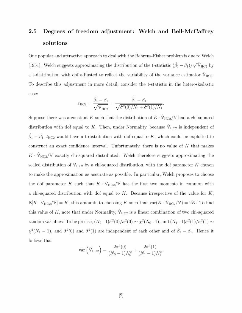
2.5 Degrees of freedom adjustment: Welch and Bell-McCaffrey
solutions
One popular and attractive approach to deal with the Behrens-Fisher problem is due to Welch
[1951]. Welch suggests approximating the distribution of the t-statistic (β1−β1)/√VHC2 by
a t-distribution with dof adjusted to reflect the variability of the variance estimator VHC2.
To describe this adjustment in more detail, consider the t-statistic in the heteroskedastic
case:
tHC2 =β1 − β1√VHC2
=β1 − β1√
σ2(0)/N0 + σ2(1)/N1
.
Suppose there was a constant K such that the distribution of K · VHC2/V had a chi-squared
distribution with dof equal to K. Then, under Normality, because VHC2 is independent of
β1 − β1, tHC2 would have a t-distribution with dof equal to K, which could be exploited to
construct an exact confidence interval. Unfortunately, there is no value of K that makes
K · VHC2/V exactly chi-squared distributed. Welch therefore suggests approximating the
scaled distribution of VHC2 by a chi-squared distribution, with the dof parameter K chosen
to make the approximation as accurate as possible. In particular, Welch proposes to choose
the dof parameter K such that K · VHC2/V has the first two moments in common with
a chi-squared distribution with dof equal to K. Because irrespective of the value for K,
E[K · VHC2/V] = K, this amounts to choosing K such that var(K · VHC2/V) = 2K. To find
this value of K, note that under Normality, VHC2 is a linear combination of two chi-squared
random variables. To be precise, (N0−1)σ2(0)/σ2(0) ∼ χ2(N0−1), and (N1−1)σ2(1)/σ2(1) ∼
χ2(N1 − 1), and σ2(0) and σ2(1) are independent of each other and of β1 − β1. Hence it
follows that
var(VHC2
)=
2σ4(0)
(N0 − 1)N20
+2σ4(1)
(N1 − 1)N21
,
[9]
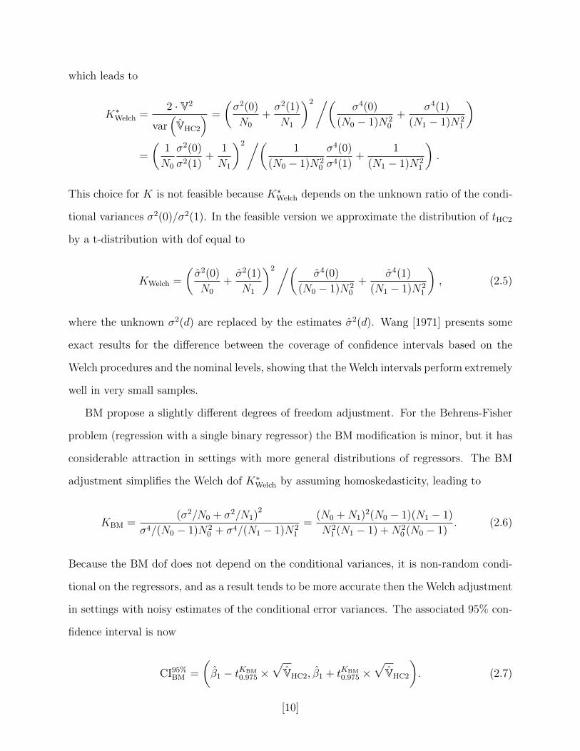
which leads to
K∗Welch =2 · V2
var(VHC2
) =
(σ2(0)
N0
+σ2(1)
N1
)2/(σ4(0)
(N0 − 1)N20
+σ4(1)
(N1 − 1)N21
)
=
(1
N0
σ2(0)
σ2(1)+
1
N1
)2/(1
(N0 − 1)N20
σ4(0)
σ4(1)+
1
(N1 − 1)N21
).
This choice for K is not feasible because K∗Welch depends on the unknown ratio of the condi-
tional variances σ2(0)/σ2(1). In the feasible version we approximate the distribution of tHC2
by a t-distribution with dof equal to
KWelch =
(σ2(0)
N0
+σ2(1)
N1
)2/(σ4(0)
(N0 − 1)N20
+σ4(1)
(N1 − 1)N21
), (2.5)
where the unknown σ2(d) are replaced by the estimates σ2(d). Wang [1971] presents some
exact results for the difference between the coverage of confidence intervals based on the
Welch procedures and the nominal levels, showing that the Welch intervals perform extremely
well in very small samples.
BM propose a slightly different degrees of freedom adjustment. For the Behrens-Fisher
problem (regression with a single binary regressor) the BM modification is minor, but it has
considerable attraction in settings with more general distributions of regressors. The BM
adjustment simplifies the Welch dof K∗Welch by assuming homoskedasticity, leading to
KBM =(σ2/N0 + σ2/N1)
2
σ4/(N0 − 1)N20 + σ4/(N1 − 1)N2
1
=(N0 +N1)
2(N0 − 1)(N1 − 1)
N21 (N1 − 1) +N2
0 (N0 − 1). (2.6)
Because the BM dof does not depend on the conditional variances, it is non-random condi-
tional on the regressors, and as a result tends to be more accurate then the Welch adjustment
in settings with noisy estimates of the conditional error variances. The associated 95% con-
fidence interval is now
CI95%BM =
(β1 − tKBM
0.975 ×√
VHC2, β1 + tKBM0.975 ×
√VHC2
). (2.7)
[10]
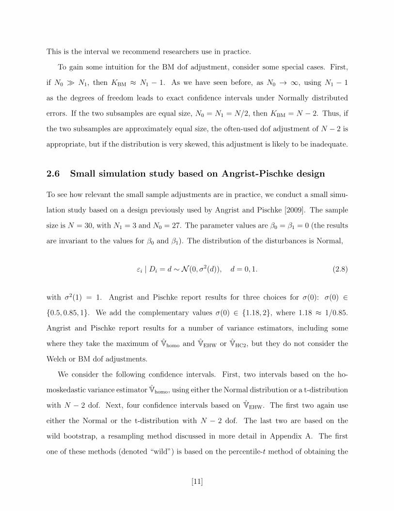
This is the interval we recommend researchers use in practice.
To gain some intuition for the BM dof adjustment, consider some special cases. First,
if N0 N1, then KBM ≈ N1 − 1. As we have seen before, as N0 → ∞, using N1 − 1
as the degrees of freedom leads to exact confidence intervals under Normally distributed
errors. If the two subsamples are equal size, N0 = N1 = N/2, then KBM = N − 2. Thus, if
the two subsamples are approximately equal size, the often-used dof adjustment of N − 2 is
appropriate, but if the distribution is very skewed, this adjustment is likely to be inadequate.
2.6 Small simulation study based on Angrist-Pischke design
To see how relevant the small sample adjustments are in practice, we conduct a small simu-
lation study based on a design previously used by Angrist and Pischke [2009]. The sample
size is N = 30, with N1 = 3 and N0 = 27. The parameter values are β0 = β1 = 0 (the results
are invariant to the values for β0 and β1). The distribution of the disturbances is Normal,
εi | Di = d ∼ N (0, σ2(d)), d = 0, 1. (2.8)
with σ2(1) = 1. Angrist and Pischke report results for three choices for σ(0): σ(0) ∈
0.5, 0.85, 1. We add the complementary values σ(0) ∈ 1.18, 2, where 1.18 ≈ 1/0.85.
Angrist and Pischke report results for a number of variance estimators, including some
where they take the maximum of Vhomo and VEHW or VHC2, but they do not consider the
Welch or BM dof adjustments.
We consider the following confidence intervals. First, two intervals based on the ho-
moskedastic variance estimator Vhomo, using either the Normal distribution or a t-distribution
with N − 2 dof. Next, four confidence intervals based on VEHW. The first two again use
either the Normal or the t-distribution with N − 2 dof. The last two are based on the
wild bootstrap, a resampling method discussed in more detail in Appendix A. The first
one of these methods (denoted “wild”) is based on the percentile-t method of obtaining the
[11]

confidence interval. The second confidence interval (denoted “wild0”) consists of all null
hypotheses H0 : β1 = β01 that were not rejected by wild bootstrap tests that impose the null
hypothesis when calculating the wild bootstrap distribution (see Appendix A for details).
This method involves a numerical search, and is therefore computationally intensive. Next,
seven confidence intervals based on VHC2, using: Normal distribution, t-distribution with
N − 2 dof, the two versions of the wild bootstrap, KWelch, K∗Welch, and KBM. We also include
a confidence interval based on VHC3 (see Appendix A for more details). Finally, we include
confidence intervals based on the maximum of Vhomo and VEHW, and on the maximum of
Vhomo and VHC2, both using the Normal distribution.
Table 1 presents the simulation results. For each of the variance estimators we report
coverage probabilities for nominal 95% confidence intervals, and the median of the standard
errors over the simulations. To make the standard errors comparable, we multiply the square
root of the variance estimators by tK0.975/t∞0.975 in cases where the confidence intervals are based
on t-distributions with K degrees of freedom. We also report the mean K∗Welch, KWelch and
KBM dof adjustments, which are substantial in these designs. For instance, in the first
design, with σ(0)/σ(1) = 0.5, the infeasible Welch dof is K∗Welch = 2.1, indicating that the
EHW standard errors may not be reliable: the dof correction leads to an adjustment in the
standard errors by a factor2 of t2.10.975/t∞0.957 = 4.11/1.96 = 2.1. Indeed, the coverage rate for
Normal-distribution confidence interval based on VEHW is 0.77, and it’s 0.82 based on the
unbiased variance estimator VHC2.
For the variance estimators included in the Angrist-Pischke design our simulation results
are consistent with theirs. However, the three confidence intervals based on the (feasible and
infeasible) Welch and BM degrees of freedom adjustments are superior in terms of coverage.
2To implement the degrees-of-freedom adjustment with non-integer dof K, we define the
t-distribution as the ratio of two random variables, one a random variable with a standard
(mean zero, unit variance) Normal distribution and and the second a random variable with
a gamma distribution with parameters α = K/2 and β = 2.
[12]

The confidence intervals based on the wild bootstrap with the null imposed also perform
well although they undercover somewhat at σ(0) = 0.5, and are very conservative and wide
at σ(0) = 2: their median length is about 45% greater than that of BM.
An attractive feature of the BM correction is that the confidence intervals have substan-
tially less variation in their width relative to the Welch confidence intervals. For instance,
with σ(0) = 1, the median widths of the confidence intervals based on KWelch and KBM are
3.5 and 3.7 (and the Welch confidence interval slightly undercovers), but the 0.95 quantile of
the widths are 7.1 and 6.5. The attempt to base the approximating chi-square distribution
on the heteroskedasticity consistent variance estimates leads to a considerable increase in
the variability of the width of the confidence intervals (this is evidenced in the variability
of KWelch, which has variance between 2.6 and 7.5 depending on the design). Moreover,
because conditional on the regressors, the BM critical value is fixed, size-adjusted power of
tests based on the BM correction coincides with that of tests based on HC2 and the Normal
distribution, while, as evidenced by the simulation results, its size properties are superior.
By construction the BM and Welch confidence intervals are symmetric around the point
estimate. The advantage of imposing symmetry is that the confidence intervals can be
reported in the form of (normalized) standard errors. On the other hand, when the error
distribution is asymmetric, imposing symmetry could result in worse performance of the BM
confidence intervals relative to some other methods that do not impose symmetry, such as
the wild bootstrap.
To investigate the importance of the assumption of the Normality and symmetry of the
errors, we also consider a design with log-Normal errors, εi | Di = d ∼ σ(d)Li, where Li is a
log-Normal random variable, recentered and rescaled so that it has mean zero and variance
one. The results are reported in Table 2. Here the BM intervals perform substantially better
than Welch intervals. The undercoverage of the remaining confidence intervals except the
wild bootstrap with the null imposed is even more severe than with Normal errors. The wild
bootstrap intervals, however, again tend to be very conservative and wide for larger values
[13]
of σ(0), although it is possible that, because they are allowed to be asymmetric around
the point estimate, they outperform the BM intervals for some other error distributions not
considered here.
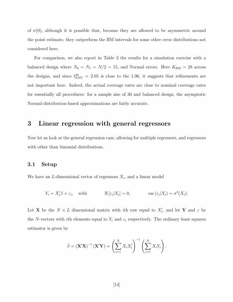
For comparison, we also report in Table 3 the results for a simulation exercise with a
balanced design where N0 = N1 = N/2 = 15, and Normal errors. Here KBM = 28 across
the designs, and since t280.975 = 2.05 is close to the 1.96, it suggests that refinements are
not important here. Indeed, the actual coverage rates are close to nominal coverage rates
for essentially all procedures: for a sample size of 30 and balanced design, the asymptotic
Normal-distribution-based approximations are fairly accurate.
3 Linear regression with general regressors
Now let us look at the general regression case, allowing for multiple regressors, and regressors
with other than binomial distributions.
3.1 Setup
We have an L-dimensional vector of regressors Xi, and a linear model
Yi = X ′iβ + εi, with E [εi|Xi] = 0, var (εi|Xi) = σ2(Xi).
Let X be the N × L dimensional matrix with ith row equal to X ′i, and let Y and ε be
the N -vectors with ith elements equal to Yi and εi respectively. The ordinary least squares
estimator is given by
β = (X′X)−1
(X′Y) =
(N∑i=1
XiX′i
)−1( N∑i=1
XiYi
).
[14]

Without assuming homoskedasticity, the exact variance for β conditional on X is
V = var(β | X) = (X′X)−1
N∑i=1
σ2(Xi)XiX′i (X′X)
−1,
with k-th diagonal element Vk. For the general regression case the EHW robust variance
estimator is
VEHW = (X′X)−1
N∑i=1
(Yi −Xiβ
)2XiX
′i (X′X)
−1,
with k-th diagonal element VEHW,k. Using a Normal distribution, the associated 95% confi-
dence interval for βk is
CI95%EHW =
(βk − 1.96×
√VEHW,k, βk + 1.96×
√VEHW,k
).
This robust variance estimator and the associated confidence intervals are widely used in
empirical work.
3.2 Bias-adjusted variance estimator
In Section 2 we discussed the bias of the robust variance estimator in the case with a single
binary regressor. In that case there was a simple modification of the EHW variance estimator
that removes all bias. In the general regression case it is not possible to remove all bias in
general. We focus on a particular adjustment for the bias first proposed by MacKinnon
and White [1985] [see also Horn et al., 1975]. In the special case with only a single binary
regressor this adjustment is identical to that used in Section 2. Let P = X(X′X)−1X′ be
the N ×N projection matrix, with i-th column denoted by Pi = X(X′X)−1Xi and (i, i)-th
element denoted by Pii = X ′i(X′X)−1Xi. Let Ω be the N × N diagonal matrix with i-th
diagonal element equal to σ2(Xi), and let eN,i be the N -vector with i-th element equal to one
and all other elements equal to zero. Let IN be the N × N identity matrix. The residuals
[15]

εi = Yi −X ′iβ can be written as
εi = εi − e′N,iPε = e′N,i(IN −P)ε, or, in vector form, ε = (IN −P)ε.
The expected value of the square of the i-th residual is
E[ε2i]
= E[(e′N,i(IN −P)ε)2
]= (eN,i −Pi)
′Ω(eN,i −Pi),
which, under homoskedasticity reduces to σ2(1−Pii). This in turn implies that ε2i /(1−Pii) is
unbiased for E [ε2i ] under homoskedasticity. This is the motivation for the variance estimator
that MacKinnon and White [1985] introduce as HC2:
VHC2 = (X′X)−1
N∑i=1
(Yi −Xiβ
)21−Pii
XiX′i (X′X)
−1. (3.1)
Suppose we want to construct a confidence interval for βk, the k-th element of β. The
variance of βk is estimated as VHC2,k, the kth diagonal element of VHC2. The 95% confidence
interval, based on the Normal approximation, is then given by
CI95%HC2 =
(βk − 1.96×
√VHC2,k, βk + 1.96×
√VHC2,k
).
3.3 Degrees of freedom adjustment
BM, building on Satterthwaite [1946], suggest approximating the distribution of the t-
statistic tHC2 = (βk − βk)/√
VHC2,k by a t-distribution instead of a Normal distribution.
Like in the binary Behrens-Fisher case, the degrees of freedom K are chosen so that under
homoskedasticity (Ω = σ2IN) the first two moments of K · (VHC2,k/Vk) are equal to those
of a chi-squared distribution with degrees of freedom equal to K. Under homoskedasticity,
VHC2 is unbiased, and thus thus E[VHC2,k] = Vk, so that the first moment of K · (VHC2,k/Vk)
is always equal to to that of a chi-squared distribution with dof equal to K. Therefore, we
[16]

choose K to match the second moment. Under Normality, VHC2,k is a linear combination
of N independent chi-squared one random variables (with some of the coefficients equal to
zero),
VHC2,k =N∑i=1
λi · Zi, where Zi ∼ χ2(1), all Zi independent,
where the weights λi are eigenvalues of the N ×N matrix σ2 ·G′G, with the i-th column of
the N ×N matrix G, equal to
Gi =1√
1−Pii
(eN,i −Pi)X′i(X
′X)−1eL,k.
Given these weights, the BM dof that match the first two moments of K · (VHC2,k/Vk) to
that of a chi-squared K distribution is given by
KBM =2 · V2
k
var(VHC2,k
) =
(N∑i=1
λi
)2/ N∑i=1
λ2i . (3.2)
The value of KBM only depends on the regressors (through the matrix G) and not on σ2
even though the weights λi do depend on σ2. In particular, the effective dof will be smaller
if the distribution of the regressors is skewed. Note also that the dof adjustment may be
different for different elements of parameter β. The resulting 95% confidence interval is
CI95%BM =
(βk + tKBM
0.025 ×√
VHC2,k, βk + tKBM0.975 ×
√VHC2,k
).
In general, the weights λi that set the moments of the chi-squared approximation equal to
those of the normalized variance are the eigenvalues of G′ΩG. These weights are not feasible,
because Ω is not known in general. The feasible version of the Sattherthwaite dof suggestion
replaces Ω by Ω = diag(ε2i /(1 − Pii)). However, because Ω is a noisy estimator of the
conditional variance, the resulting confidence intervals are often substantially conservative.
By basing the dof calculation on the homoskedastic case with Ω = σ2 ·IN , the BM adjustment
[17]

avoids this problem.
If there is a single binary regressor, the BM solution for the general case (3.2) reduces to
that in the binary case, (2.6). Similarly, the infeasible Sattherthwaite solution, based on the
eigenvalues of GΩG, reduces to the infeasible Welch solution K∗Welch. In contrast, applying
the feasible Sattherthwaite solution to the case with a binary regressor does not lead to the
feasible Welch solution because the feasible Welch solution implicitly uses an estimator for
Ω different from Ω.
The performance of the Sattherthwaite and BM confidence intervals is similar to that of
the Welch and BM confidence intervals in the binary case.3 In particular, if the design of
regressors is skewed (for example, if the regressor of interest has a log-Normal distribution),
then the robust variance estimators VEHW and the bias-adjusted version VHC2 based on a
normal distribution or a t-distribution with N − 2 dof may undercover substantially even
when N ≈ 100. In contrast, the Sattherthwaite and BM confidence intervals control size even
in small samples, because any skewness is captured in the matrix G, leading to appropriate
dof adjustments. The KBM dof adjustment leads to much narrower confidence intervals with
much less variation, so again that is the superior choice in this setting.
4 Robust variance estimators with clustering
In this section we discuss the extensions of the variance estimators discussed in the previous
sections to the case with clustering. The model is:
Yi = X ′iβ + εi, (4.1)
There are S clusters. In cluster s the number of units is Ns, with the overall sample size
N =∑S
s=1Ns. Let Si ∈ 1, . . . , S denote the cluster unit i belongs to. We assume that the
errors εi are uncorrelated between clusters, but there may be arbitrary correlation within a
3See an earlier version of this paper [Imbens and Kolesar, 2012] for simulation evidence.
[18]

cluster,
E[ε | X] = 0, E[εε′ | X] = Ω, Ωij =
ωij if Si = Sj,
0 otherwise.
If ωij = 0 for i 6= j (that is, each unit is in its own cluster), the setup reduces to that in
Section 3.
Let β be the least squares estimator, and let εi = Yi − X ′iβ be the residual. Let εs be
the Ns dimensional vector with the residuals in cluster s, let Xs the Ns×L matrix with ith
row equal to the value of X ′i for the ith unit in cluster s, and let X be the N × L matrix
constructed by stacking X1 through XS. Define the N ×Ns matrix Ps = X(X′X)−1X′s, the
Ns ×Ns matrix Pss = Xs(X′X)−1X′s, and define the N ×Ns matrix (IN −P)s to consist of
the Ns columns of the N ×N matrix (IN −P) corresponding to cluster s.
The exact variance of β conditional on X is given by
V = (X′X)−1X′ΩX(X′X)−1.
The standard robust variance estimator, due to Liang and Zeger [1986] [see also Diggle et al.,
2002], is
VLZ = (X′X)−1
S∑s=1
X′sεsε′sXs (X′X)
−1.
Often a simple multiplicative adjustment is used, for example in STATA, to reduce the bias
of the LZ variance estimator:
VSTATA =N − 1
N − L· S
S − 1· (X′X)
−1S∑s=1
X′sεsε′sXs (X′X)
−1.
The main component of this adjustment is typically the S/(S − 1) factor, because in many
applications, (N − 1)/(N − L) is close to one.
The bias-reduction modification developed by Bell and McCaffrey [2002], analogous to
[19]

the HC2 bias reduction of the original Eicker-Huber-White variance estimator, is
VLZ2 = (X′X)−1
S∑s=1
X′s(INs −Pss)−1/2εsε
′s(INs −Pss)
−1/2Xs (X′X)−1,
where (INs − Pss)−1/2 is the inverse of the symmetric square root of (INs − Pss). For each
of the variance estimators, let VLZ,k, VSTATA,k and VLZ2,k are the k-th diagonal elements of
VLZ, VSTATA and VLZ2 respectively.
To define the degrees-of-freedom adjustment, let G denote the N × S matrix with s-th
column equal to the N -vector
Gs = (IN −P)s(INs −Pss)−1/2Xs (X′X)
−1eL,k.
Then the dof adjustment is given by
KBM =
(∑Ni=1 λi
)2∑N
i=1 λ2i
.
where λi are the eigenvalues of G′G. If each unit is in its own cluster (so there is no
clustering), this adjustment reduces to the adjustment given in (3.2). The 95% confidence
interval is given by
CI95%cluster,BM =
(βk + tKBM
0.025 ×√
VLZ2,k, βk + tKBM0.975 ×
√VLZ2,k
). (4.2)
We also consider a slightly different version of the dof adjustment. In principle, we would
like to use the eigenvalues of the matrix G′ΩG, so that the first two moments of K ·VLZ2,k/Vk
match that of χ2(K). It is difficult to estimate Ω accurately without any restrictions, which
motivated BM to use σ2 · IN instead. In the clustering case, however, it is attractive to put
a random-effects structure on the errors as in Moulton [1986, 1990] and estimate a model
[20]

for Ω where
Ωij =
σ2ε if i = j,
ρ if i 6= j, Si = Sj.
0 otherwise
We estimate σν as the average of the product of the residuals for units with Si = Sj, and
i 6= j
ρ =1
m−N
S∑s=1
∑i : Si=s
∑j : Sj=s
εiεj −N∑i=1
ε2i
,
where m =∑S
s=1N2s , and Ns is the number of observations in cluster S, and we estimate σ2
ε
as the average of the square of the residuals, σ2ε = N−1
∑Ni=1 ε
2i . We then calculate the λi as
the eigenvalues of G′ΩG, and set
KIK =
(∑Ni=1 λi
)2∑N
i=1 λ2i
.
4.1 Small simulation study
We carry out a small simulation study. The first sets of designs is corresponds to the designs
first used in Cameron et al. [2008]. The baseline model (design I) is the same as in (4.1),
with a scalar regressor:
Yi = β0 + β1 ·Xi + εi,
with β0 = β1 = 0, Xi = VSi + Wi and εi = νSi + ηi, with Vs, Wi, νs, ηi are all Normally
distributed, with mean zero and unit variance. There there are S = 10 clusters, with Ns = 30
units in each cluster. In design II, we have S = 5 clusters, again with Ns = 30 in each cluster.
In design III, there there are again S = 10 clusters, half with Ns = 10 and half with Ns = 50.
In the fourth and fifth design we return to the design with S = 10 clusters and Ns = 30 units
per cluster. In the design IV we introduce heteroskedasticity, with ηi|X ∼ N(0, 0.9X2i ), and
[21]
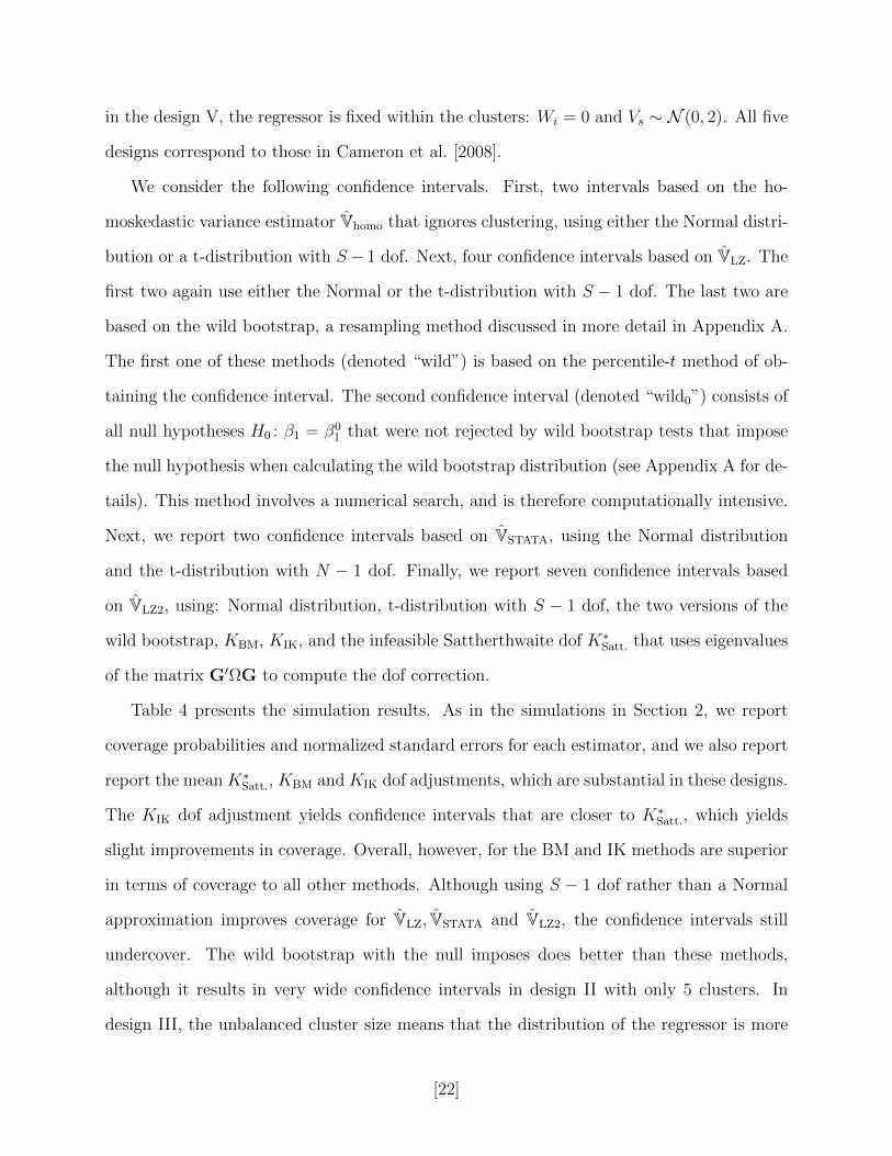
in the design V, the regressor is fixed within the clusters: Wi = 0 and Vs ∼ N (0, 2). All five
designs correspond to those in Cameron et al. [2008].
We consider the following confidence intervals. First, two intervals based on the ho-
moskedastic variance estimator Vhomo that ignores clustering, using either the Normal distri-
bution or a t-distribution with S− 1 dof. Next, four confidence intervals based on VLZ. The
first two again use either the Normal or the t-distribution with S − 1 dof. The last two are
based on the wild bootstrap, a resampling method discussed in more detail in Appendix A.
The first one of these methods (denoted “wild”) is based on the percentile-t method of ob-
taining the confidence interval. The second confidence interval (denoted “wild0”) consists of
all null hypotheses H0 : β1 = β01 that were not rejected by wild bootstrap tests that impose
the null hypothesis when calculating the wild bootstrap distribution (see Appendix A for de-
tails). This method involves a numerical search, and is therefore computationally intensive.
Next, we report two confidence intervals based on VSTATA, using the Normal distribution
and the t-distribution with N − 1 dof. Finally, we report seven confidence intervals based
on VLZ2, using: Normal distribution, t-distribution with S − 1 dof, the two versions of the
wild bootstrap, KBM, KIK, and the infeasible Sattherthwaite dof K∗Satt. that uses eigenvalues
of the matrix G′ΩG to compute the dof correction.
Table 4 presents the simulation results. As in the simulations in Section 2, we report
coverage probabilities and normalized standard errors for each estimator, and we also report
report the mean K∗Satt., KBM and KIK dof adjustments, which are substantial in these designs.
The KIK dof adjustment yields confidence intervals that are closer to K∗Satt., which yields
slight improvements in coverage. Overall, however, for the BM and IK methods are superior
in terms of coverage to all other methods. Although using S − 1 dof rather than a Normal
approximation improves coverage for VLZ, VSTATA and VLZ2, the confidence intervals still
undercover. The wild bootstrap with the null imposes does better than these methods,
although it results in very wide confidence intervals in design II with only 5 clusters. In
design III, the unbalanced cluster size means that the distribution of the regressor is more
[22]
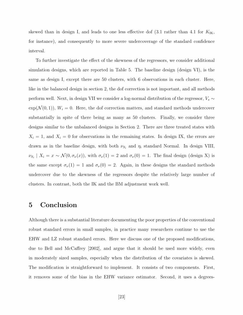
skewed than in design I, and leads to one less effective dof (3.1 rather than 4.1 for KIK,
for instance), and consequently to more severe undercoverage of the standard confidence
interval.
To further investigate the effect of the skewness of the regressors, we consider additional
simulation designs, which are reported in Table 5. The baseline design (design VI), is the
same as design I, except there are 50 clusters, with 6 observations in each cluster. Here,
like in the balanced design in section 2, the dof correction is not important, and all methods
perform well. Next, in design VII we consider a log-normal distribution of the regressor, Vs ∼
exp(N (0, 1)), Wi = 0. Here, the dof correction matters, and standard methods undercover
substantially in spite of there being as many as 50 clusters. Finally, we consider three
designs similar to the unbalanced designs in Section 2. There are three treated states with
Xi = 1, and Xi = 0 for observations in the remaining states. In design IX, the errors are
drawn as in the baseline design, with both νSi and ηi standard Normal. In design VIII,
νSi | Xi = x ∼ N (0, σν(x)), with σν(1) = 2 and σν(0) = 1. The final design (design X) is
the same except σν(1) = 1 and σν(0) = 2. Again, in these designs the standard methods
undercover due to the skewness of the regressors despite the relatively large number of
clusters. In contrast, both the IK and the BM adjustment work well.
5 Conclusion
Although there is a substantial literature documenting the poor properties of the conventional
robust standard errors in small samples, in practice many researchers continue to use the
EHW and LZ robust standard errors. Here we discuss one of the proposed modifications,
due to Bell and McCaffrey [2002], and argue that it should be used more widely, even
in moderately sized samples, especially when the distribution of the covariates is skewed.
The modification is straightforward to implement. It consists of two components. First,
it removes some of the bias in the EHW variance estimator. Second, it uses a degrees-
[23]

of-freedom adjustment that matches the moments of the variance estimator to one of a
chi-squared distribution. The dof adjustment depends on the sample size and the joint
distribution of the covariates, and differs by covariate. We discuss the connection to the
Behrens-Fisher problem, and suggest a minor modification for the case with clustering.
[24]

References
Joshua D. Angrist and Jorn-Steffen Pischke. Mostly Harmless Econometrics: An Empiricist’s
Companion. Princeton University Press, Princeton, NJ, 2009.
Walter U. Behrens. Ein beitrag zur fehlerberechnung bei wenigen beobachtungen. Land-
wirtschaftliche Jahrbucher, 68:807–837, 1929.
Robert M. Bell and Daniel F. McCaffrey. Bias reduction in standard errors for linear regres-
sion with multi-stage samples. Survey Methodology, 28(2):169–181, 2002.
A. Colin Cameron, Jonah B. Gelbach, and Douglas L. Miller. Bootstrap-based improvements
for inference with clustered errors. The Review of Economics and Statistics, 90(3):414–427,
2008.
Andrew Chesher and Ian Jewitt. The bias of a heteroskedasticity consistent covariance
matrix estimator. Econometrica, 55(5):1217–1222, 1987.
Russell Davidson and Emmanuel Flachaire. The wild bootstrap, tamed at last. Journal of
Econometrics, 146(1):162–169, September 2008.
Peter Diggle, Patrick Heagerty, Kung-Yee Liang, and Scott L. Zeger. Analysis of longitudinal
data. Oxford University Press, Oxford, 2002.
Stephen G. Donald and Kevin Lang. Inference with difference-in-differences and other panel
data. The Review of Economics and Statistics, 89(2):221–233, May 2007.
Friedhelm Eicker. Limit theorems for regressions with unequal and dependent errors. In
Lucien M. Le Cam and Jerzy Neyman, editors, Proceedings of the Berkeley Symposium
on Mathematical Statistics and Probability, volume 1, pages 59–82, Berkeley, CA, 1967.
University of California Press.
Ronald Aylmer Fisher. The comparison of samples with possibly unequal variances. Annals
of Eugenics, 9(2):174–180, 1939.
[25]
Jerry A. Hausman and Christopher J. Palmer. Heteroskedasticity-robust inference in finite
samples. NBER Working Paper 17698, 2011.
Susan D. Horn, Roger A. Horn, and David B. Duncan. Estimating heteroscedastic variances
in linear models. Journal of the American Statistical Association, 70(350):380–385, 1975.
Peter J. Huber. The behavior of maximum likelihood estimates under nonstandard con-
ditions. In Lucien M. Le Cam and Jerzy Neyman, editors, Proceedings of the Berkeley
Symposium on Mathematical Statistics and Probability, volume 1, pages 221–233, Berkeley,
CA, 1967. University of California Press.
Rustam Ibragimov and Ulrich K. Muller. t-statistic based correlation and heterogeneity
robust inference. Journal of Business & Economic Statistics, 28(4):453–468, 2010.
Guido W. Imbens and Michal Kolesar. Robust standard errors in small samples: Some
practical advice. NBER Working Paper 18478, 2012.
Erich L. Lehmann and Joseph P. Romano. Testing statistical hypotheses. Springer, third
edition, 2005.
Kung-Yee Liang and Scott L. Zeger. Longitudinal data analysis for generalized linear models.
Biometrika, 73(1):13–22, 1986.
Regina Y. Liu. Bootstrap procedures under some non-iid models. The Annals of Statistics,
16(4):1696–1708, 1988.
James G. MacKinnon. Bootstrap inference in econometrics. The Canadian Journal of Eco-
nomics / Revue Canadienne d’Economique, 35(4):615–645, 2002.
James G. MacKinnon. Thirty years of heteroskedasticity-robust inference. In Xaiohong Chen
and Norman R. Swanson, editors, Recent Advances and Future Directions in Causality,
Prediction, and Specification Analysis, pages 437–461. Springer, New York, 2012.
[26]
James G. MacKinnon and Halbert White. Some heteroskedasticity-consistent covariance
matrix estimators with improved finite sample properties. Journal of Econometrics, 29
(3):305–325, 1985.
Enno Mammen. Bootstrap and wild bootstrap for high dimensional linear models. The
Annals of Statistics, 21(1):255–285, 1993.
Brent R. Moulton. Random group effects and the precision of regression estimates. Journal
of Econometrics, 32(3):385–397, 1986.
Brent R. Moulton. An illustration of a pitfall in estimating the effects of aggregate variables
on micro units. The Review of Economics and Statistics, 72(2):334–338, 1990.
F. E. Satterthwaite. An approximate distribution of estimates of variance components.
Biometrics Bulletin, 2(6):110–114, 1946.
Henry Scheffe. Practical solutions of the behrens-fisher problem. Journal of the American
Statistical Association, 65(332):1501–1508, 1970.
Ying Y. Wang. Probabilities of the type i errors of the welch tests for the behrens-fisher
problem. Journal of the American Statistical Association, 66(335):605–608, 1971.
B. L. Welch. On the comparison of several mean values: An alternative approach. Biometrika,
38(3):330–336, 1951.
Halbert White. A heteroskedasticity-consistent covariance matrix estimator and a direct test
for heteroskedasticity. Econometrica, 48(4):817–838, 1980.
[27]
Appendix A Other methods
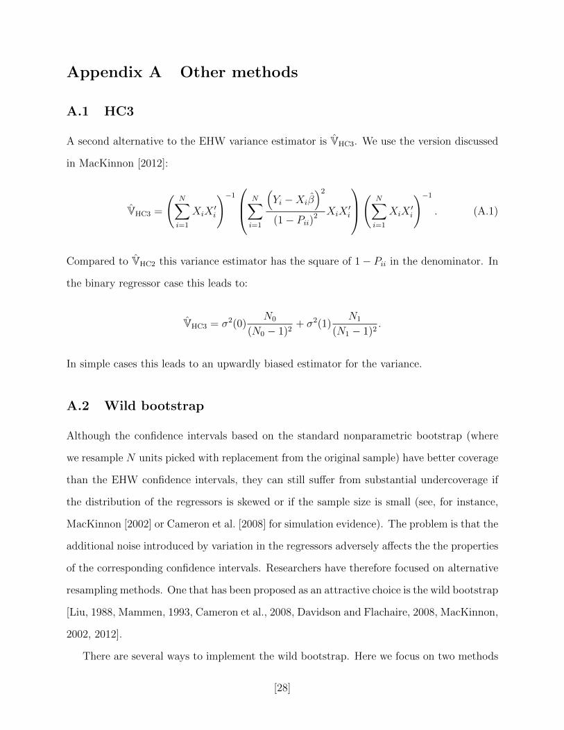
A.1 HC3
A second alternative to the EHW variance estimator is VHC3. We use the version discussed
in MacKinnon [2012]:
VHC3 =
(N∑i=1
XiX′i
)−1 N∑i=1
(Yi −Xiβ
)2(1− Pii)2
XiX′i
( N∑i=1
XiX′i
)−1. (A.1)
Compared to VHC2 this variance estimator has the square of 1− Pii in the denominator. In
the binary regressor case this leads to:
VHC3 = σ2(0)N0
(N0 − 1)2+ σ2(1)
N1
(N1 − 1)2.
In simple cases this leads to an upwardly biased estimator for the variance.
A.2 Wild bootstrap
Although the confidence intervals based on the standard nonparametric bootstrap (where
we resample N units picked with replacement from the original sample) have better coverage
than the EHW confidence intervals, they can still suffer from substantial undercoverage if
the distribution of the regressors is skewed or if the sample size is small (see, for instance,
MacKinnon [2002] or Cameron et al. [2008] for simulation evidence). The problem is that the
additional noise introduced by variation in the regressors adversely affects the the properties
of the corresponding confidence intervals. Researchers have therefore focused on alternative
resampling methods. One that has been proposed as an attractive choice is the wild bootstrap
[Liu, 1988, Mammen, 1993, Cameron et al., 2008, Davidson and Flachaire, 2008, MacKinnon,
2002, 2012].
There are several ways to implement the wild bootstrap. Here we focus on two methods
[28]

based on resampling the t statistic. We first describe the two methods in the regression
setting, and then in the cluster setting.
Suppose that we wish to test the hypothesis that H0 : β` = β0` . Let β be the least squares
estimate in the original sample, let ε = Yi − X ′iβ be the estimated residuals, and let V be
a variance estimator, either VEHW, or VHC2, or VHC3. Let t = (β` − β0` )/√V denote the
t-statistic.
In the wild bootstrap the regressor values are fixed in the resampling. For the first
method, the value of the i-th outcome in the bth bootstrap replication is redrawn as
Yi,b = X ′iβ1 + Ui,b · εi,
where Ui,b is a binary random variable with pr(Ui,b = 1) = pr(Ui,b = −1) = 1/2, with Ui,b
independent across i and b. (Other distributions for Ui,b are also possible; we focus on this
particular choice following Cameron et al. [2008].) The second method we consider “imposes
the null” when redrawing the outcomes. In particular, letting β(β0` ) denote the value of
the restricted least squares estimate that minimizes the sum of squared residuals subject to
β` = β0` . Then the i-th outcome in the bth bootstrap replication is redrawn as
Yi,b = X ′iβ(β0` ) + Ui,b · (Yi −X ′iβ(β0
` ))
Once the new outcomes are redrawn, for each bootstrap sample (Yi,b, Xi)ni=1, calculate the
t-statistic as
t1b =βb,` − β`√
Vb
,
if using the first method, or as
t2b(β0` ) =
βb,` − β0`√
Vb
,
if using the second method, where Vb is some variance estimator. We focus on a symmetric
version of the critical values. In particular, over all the bootstrap samples, set the critical
[29]

value to q0.95(|t1|), the 0.95 quantile of the distribution of |t1b | (or q0.95(|t2(β0)|) if using the
second method). Reject the null if |t| is greater than the critical value.
The first method does not impose the null hypothesis when redrawing the outcomes,
or calculating the critical value, so that q0.95(|t1|) does not depend on which β0` is being
tested. Therefore, to construct a 95% confidence interval, we simply replace the standard
1.96 critical value by qwild0.95 ,
CI95%wild =
(β` − q0.95(|t1|)×
√V, β1 + q0.95(|t1|)×
√V). (A.2)
We denote this confidence interval as “wild” in the simulations.For the second method, the
confidence interval consists of all points b such that the null H0 : β` = b is not rejected:
CI95%wild0 =
b : |β` − b|/
√ˆV ≤ qwild
0.95 (t2(b))
.
We denote this confidence interval as “wild0” in the simulations. Because constructing this
confidence interval involves testing many null hypotheses, the method it is computationally
intensive. The wild bootstrap standard errors reported in the tables defined as the length of
the bootstrap confidence interval divided by 2× 1.96.
For the cluster version of the wild bootstrap, the bootstrap variable Us,b is indexed by the
cluster only. Again the distribution of Us,b is binary with values −1 and 1, and probability
pr(Us,b = 1) = pr(Us,b = −1) = 0.5. The bootstrap value for the outcome for unit i in cluster
s is then
Yis,b = X ′isβ + Us,b · εis
for the first method, and
Yis,b = X ′isβ(β0,`) + Us,b · (Yis −X ′isβ(β0,`))
[30]

for the second method that imposes the null, with the covariates Xis remaining fixed across
the bootstrap replications.
[31]
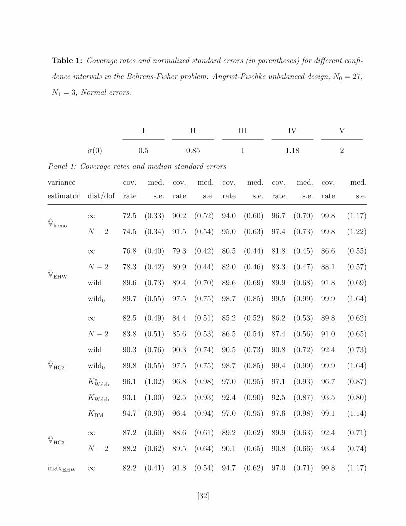
Table 1: Coverage rates and normalized standard errors (in parentheses) for different confi-
dence intervals in the Behrens-Fisher problem. Angrist-Pischke unbalanced design, N0 = 27,
N1 = 3, Normal errors.
I II III IV V
σ(0) 0.5 0.85 1 1.18 2
Panel 1: Coverage rates and median standard errors
variance cov. med. cov. med. cov. med. cov. med. cov. med.
estimator dist/dof rate s.e. rate s.e. rate s.e. rate s.e. rate s.e.
Vhomo
∞ 72.5 (0.33) 90.2 (0.52) 94.0 (0.60) 96.7 (0.70) 99.8 (1.17)
N − 2 74.5 (0.34) 91.5 (0.54) 95.0 (0.63) 97.4 (0.73) 99.8 (1.22)
VEHW
∞ 76.8 (0.40) 79.3 (0.42) 80.5 (0.44) 81.8 (0.45) 86.6 (0.55)
N − 2 78.3 (0.42) 80.9 (0.44) 82.0 (0.46) 83.3 (0.47) 88.1 (0.57)
wild 89.6 (0.73) 89.4 (0.70) 89.6 (0.69) 89.9 (0.68) 91.8 (0.69)
wild0 89.7 (0.55) 97.5 (0.75) 98.7 (0.85) 99.5 (0.99) 99.9 (1.64)
VHC2
∞ 82.5 (0.49) 84.4 (0.51) 85.2 (0.52) 86.2 (0.53) 89.8 (0.62)
N − 2 83.8 (0.51) 85.6 (0.53) 86.5 (0.54) 87.4 (0.56) 91.0 (0.65)
wild 90.3 (0.76) 90.3 (0.74) 90.5 (0.73) 90.8 (0.72) 92.4 (0.73)
wild0 89.8 (0.55) 97.5 (0.75) 98.7 (0.85) 99.4 (0.99) 99.9 (1.64)
K∗Welch 96.1 (1.02) 96.8 (0.98) 97.0 (0.95) 97.1 (0.93) 96.7 (0.87)
KWelch 93.1 (1.00) 92.5 (0.93) 92.4 (0.90) 92.5 (0.87) 93.5 (0.80)
KBM 94.7 (0.90) 96.4 (0.94) 97.0 (0.95) 97.6 (0.98) 99.1 (1.14)
VHC3
∞ 87.2 (0.60) 88.6 (0.61) 89.2 (0.62) 89.9 (0.63) 92.4 (0.71)
N − 2 88.2 (0.62) 89.5 (0.64) 90.1 (0.65) 90.8 (0.66) 93.4 (0.74)
maxEHW ∞ 82.2 (0.41) 91.8 (0.54) 94.7 (0.62) 97.0 (0.71) 99.8 (1.17)
[32]
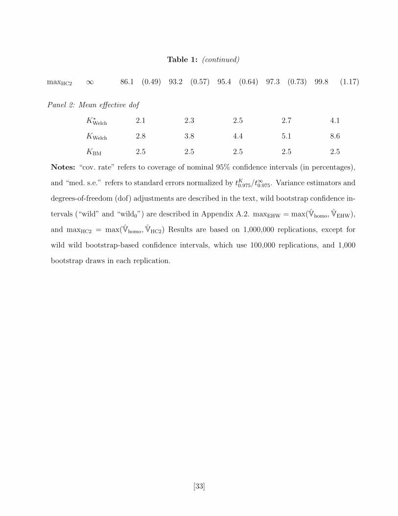
Table 1: (continued)
maxHC2 ∞ 86.1 (0.49) 93.2 (0.57) 95.4 (0.64) 97.3 (0.73) 99.8 (1.17)
Panel 2: Mean effective dof
K∗Welch 2.1 2.3 2.5 2.7 4.1
KWelch 2.8 3.8 4.4 5.1 8.6
KBM 2.5 2.5 2.5 2.5 2.5
Notes: “cov. rate” refers to coverage of nominal 95% confidence intervals (in percentages),
and “med. s.e.” refers to standard errors normalized by tK0.975/t∞0.975. Variance estimators and
degrees-of-freedom (dof) adjustments are described in the text, wild bootstrap confidence in-
tervals (“wild” and “wild0”) are described in Appendix A.2. maxEHW = max(Vhomo, VEHW),
and maxHC2 = max(Vhomo, VHC2) Results are based on 1,000,000 replications, except for
wild wild bootstrap-based confidence intervals, which use 100,000 replications, and 1,000
bootstrap draws in each replication.
[33]
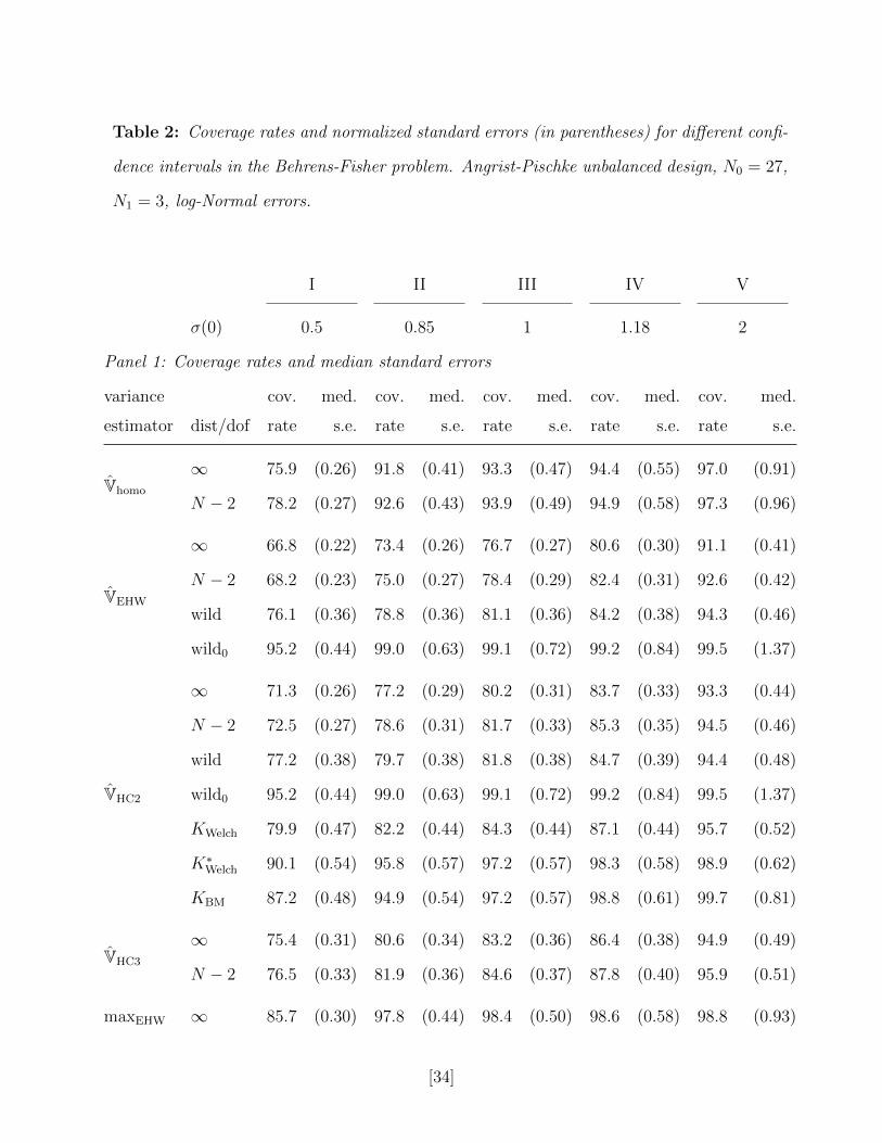
Table 2: Coverage rates and normalized standard errors (in parentheses) for different confi-
dence intervals in the Behrens-Fisher problem. Angrist-Pischke unbalanced design, N0 = 27,
N1 = 3, log-Normal errors.
I II III IV V
σ(0) 0.5 0.85 1 1.18 2
Panel 1: Coverage rates and median standard errors
variance cov. med. cov. med. cov. med. cov. med. cov. med.
estimator dist/dof rate s.e. rate s.e. rate s.e. rate s.e. rate s.e.
Vhomo
∞ 75.9 (0.26) 91.8 (0.41) 93.3 (0.47) 94.4 (0.55) 97.0 (0.91)
N − 2 78.2 (0.27) 92.6 (0.43) 93.9 (0.49) 94.9 (0.58) 97.3 (0.96)
VEHW
∞ 66.8 (0.22) 73.4 (0.26) 76.7 (0.27) 80.6 (0.30) 91.1 (0.41)
N − 2 68.2 (0.23) 75.0 (0.27) 78.4 (0.29) 82.4 (0.31) 92.6 (0.42)
wild 76.1 (0.36) 78.8 (0.36) 81.1 (0.36) 84.2 (0.38) 94.3 (0.46)
wild0 95.2 (0.44) 99.0 (0.63) 99.1 (0.72) 99.2 (0.84) 99.5 (1.37)
VHC2
∞ 71.3 (0.26) 77.2 (0.29) 80.2 (0.31) 83.7 (0.33) 93.3 (0.44)
N − 2 72.5 (0.27) 78.6 (0.31) 81.7 (0.33) 85.3 (0.35) 94.5 (0.46)
wild 77.2 (0.38) 79.7 (0.38) 81.8 (0.38) 84.7 (0.39) 94.4 (0.48)
wild0 95.2 (0.44) 99.0 (0.63) 99.1 (0.72) 99.2 (0.84) 99.5 (1.37)
KWelch 79.9 (0.47) 82.2 (0.44) 84.3 (0.44) 87.1 (0.44) 95.7 (0.52)
K∗Welch 90.1 (0.54) 95.8 (0.57) 97.2 (0.57) 98.3 (0.58) 98.9 (0.62)
KBM 87.2 (0.48) 94.9 (0.54) 97.2 (0.57) 98.8 (0.61) 99.7 (0.81)
VHC3
∞ 75.4 (0.31) 80.6 (0.34) 83.2 (0.36) 86.4 (0.38) 94.9 (0.49)
N − 2 76.5 (0.33) 81.9 (0.36) 84.6 (0.37) 87.8 (0.40) 95.9 (0.51)
maxEHW ∞ 85.7 (0.30) 97.8 (0.44) 98.4 (0.50) 98.6 (0.58) 98.8 (0.93)
[34]

Table 2: (continued)
maxHC2 ∞ 86.9 (0.33) 98.5 (0.46) 99.0 (0.52) 99.2 (0.60) 99.3 (0.94)
Panel 2: Mean effective dof
K∗Welch 2.1 2.3 2.5 2.7 4.1
KWelch 4.9 7.5 8.5 9.7 14.0
KBM 2.5 2.5 2.5 2.5 2.5
Notes: “cov. rate” refers to coverage of nominal 95% confidence intervals (in percentages),
and “med. s.e.” refers to standard errors normalized by tK0.975/t∞0.975. Variance estimators and
degrees-of-freedom (dof) adjustments are described in the text, wild bootstrap confidence in-
tervals (“wild” and “wild0”) are described in Appendix A.2. maxEHW = max(Vhomo, VEHW),
and maxHC2 = max(Vhomo, VHC2) Results are based on 1,000,000 replications, except for
wild wild bootstrap-based confidence intervals, which use 100,000 replications, and 1,000
bootstrap draws in each replication.
[35]
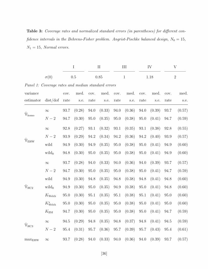
Table 3: Coverage rates and normalized standard errors (in parentheses) for different con-
fidence intervals in the Behrens-Fisher problem. Angrist-Pischke balanced design, N0 = 15,
N1 = 15, Normal errors.
I II III IV V
σ(0) 0.5 0.85 1 1.18 2
Panel 1: Coverage rates and median standard errors
variance cov. med. cov. med. cov. med. cov. med. cov. med.
estimator dist/dof rate s.e. rate s.e. rate s.e. rate s.e. rate s.e.
Vhomo
∞ 93.7 (0.28) 94.0 (0.33) 94.0 (0.36) 94.0 (0.39) 93.7 (0.57)
N − 2 94.7 (0.30) 95.0 (0.35) 95.0 (0.38) 95.0 (0.41) 94.7 (0.59)
VEHW
∞ 92.8 (0.27) 93.1 (0.32) 93.1 (0.35) 93.1 (0.38) 92.8 (0.55)
N − 2 93.9 (0.29) 94.2 (0.34) 94.2 (0.36) 94.2 (0.40) 93.9 (0.57)
wild 94.9 (0.30) 94.9 (0.35) 95.0 (0.38) 95.0 (0.41) 94.9 (0.60)
wild0 94.8 (0.30) 95.0 (0.35) 95.0 (0.38) 95.0 (0.41) 94.9 (0.60)
VHC2
∞ 93.7 (0.28) 94.0 (0.33) 94.0 (0.36) 94.0 (0.39) 93.7 (0.57)
N − 2 94.7 (0.30) 95.0 (0.35) 95.0 (0.38) 95.0 (0.41) 94.7 (0.59)
wild 94.9 (0.30) 94.8 (0.35) 94.8 (0.38) 94.8 (0.41) 94.8 (0.60)
wild0 94.9 (0.30) 95.0 (0.35) 94.9 (0.38) 95.0 (0.41) 94.8 (0.60)
KWelch 95.0 (0.30) 95.1 (0.35) 95.1 (0.38) 95.1 (0.41) 95.0 (0.60)
K∗Welch 95.0 (0.30) 95.0 (0.35) 95.0 (0.38) 95.0 (0.41) 95.0 (0.60)
KBM 94.7 (0.30) 95.0 (0.35) 95.0 (0.38) 95.0 (0.41) 94.7 (0.59)
VHC3
∞ 94.5 (0.29) 94.8 (0.35) 94.8 (0.37) 94.8 (0.41) 94.5 (0.59)
N − 2 95.4 (0.31) 95.7 (0.36) 95.7 (0.39) 95.7 (0.43) 95.4 (0.61)
maxEHW ∞ 93.7 (0.28) 94.0 (0.33) 94.0 (0.36) 94.0 (0.39) 93.7 (0.57)
[36]
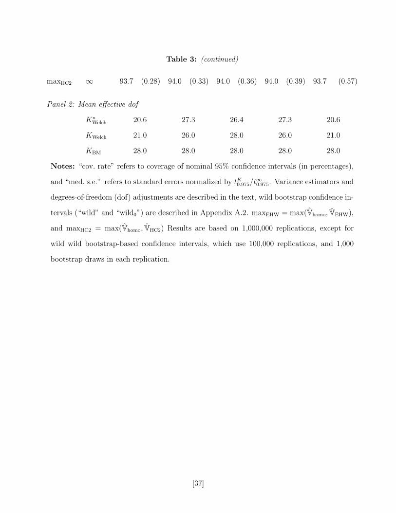
Table 3: (continued)
maxHC2 ∞ 93.7 (0.28) 94.0 (0.33) 94.0 (0.36) 94.0 (0.39) 93.7 (0.57)
Panel 2: Mean effective dof
K∗Welch 20.6 27.3 26.4 27.3 20.6
KWelch 21.0 26.0 28.0 26.0 21.0
KBM 28.0 28.0 28.0 28.0 28.0
Notes: “cov. rate” refers to coverage of nominal 95% confidence intervals (in percentages),
and “med. s.e.” refers to standard errors normalized by tK0.975/t∞0.975. Variance estimators and
degrees-of-freedom (dof) adjustments are described in the text, wild bootstrap confidence in-
tervals (“wild” and “wild0”) are described in Appendix A.2. maxEHW = max(Vhomo, VEHW),
and maxHC2 = max(Vhomo, VHC2) Results are based on 1,000,000 replications, except for
wild wild bootstrap-based confidence intervals, which use 100,000 replications, and 1,000
bootstrap draws in each replication.
[37]
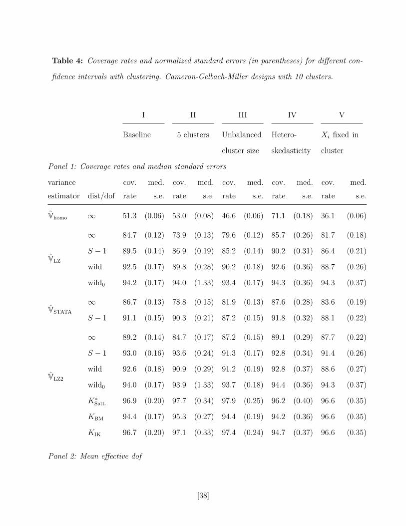
Table 4: Coverage rates and normalized standard errors (in parentheses) for different con-
fidence intervals with clustering. Cameron-Gelbach-Miller designs with 10 clusters.
I II III IV V
Baseline 5 clusters Unbalanced
cluster size
Hetero-
skedasticity
Xi fixed in
cluster
Panel 1: Coverage rates and median standard errors
variance cov. med. cov. med. cov. med. cov. med. cov. med.
estimator dist/dof rate s.e. rate s.e. rate s.e. rate s.e. rate s.e.
Vhomo ∞ 51.3 (0.06) 53.0 (0.08) 46.6 (0.06) 71.1 (0.18) 36.1 (0.06)
VLZ
∞ 84.7 (0.12) 73.9 (0.13) 79.6 (0.12) 85.7 (0.26) 81.7 (0.18)
S − 1 89.5 (0.14) 86.9 (0.19) 85.2 (0.14) 90.2 (0.31) 86.4 (0.21)
wild 92.5 (0.17) 89.8 (0.28) 90.2 (0.18) 92.6 (0.36) 88.7 (0.26)
wild0 94.2 (0.17) 94.0 (1.33) 93.4 (0.17) 94.3 (0.36) 94.3 (0.37)
VSTATA
∞ 86.7 (0.13) 78.8 (0.15) 81.9 (0.13) 87.6 (0.28) 83.6 (0.19)
S − 1 91.1 (0.15) 90.3 (0.21) 87.2 (0.15) 91.8 (0.32) 88.1 (0.22)
VLZ2
∞ 89.2 (0.14) 84.7 (0.17) 87.2 (0.15) 89.1 (0.29) 87.7 (0.22)
S − 1 93.0 (0.16) 93.6 (0.24) 91.3 (0.17) 92.8 (0.34) 91.4 (0.26)
wild 92.6 (0.18) 90.9 (0.29) 91.2 (0.19) 92.8 (0.37) 88.6 (0.27)
wild0 94.0 (0.17) 93.9 (1.33) 93.7 (0.18) 94.4 (0.36) 94.3 (0.37)
K∗Satt. 96.9 (0.20) 97.7 (0.34) 97.9 (0.25) 96.2 (0.40) 96.6 (0.35)
KBM 94.4 (0.17) 95.3 (0.27) 94.4 (0.19) 94.2 (0.36) 96.6 (0.35)
KIK 96.7 (0.20) 97.1 (0.33) 97.4 (0.24) 94.7 (0.37) 96.6 (0.35)
Panel 2: Mean effective dof
[38]

Table 4: (continued)
K∗Satt. 4.0 2.3 2.9 4.6 3.4
KBM 6.6 3.3 5.1 6.6 3.4
KIK 4.1 2.4 3.1 5.7 3.4
Notes: “cov. rate” refers to coverage of nominal 95% confidence intervals (in percentages),
and “med. s.e.” refers to standard errors normalized by tK0.975/t∞0.975. Variance estimators and
degrees-of-freedom (dof) adjustments are described in the text, wild bootstrap confidence
intervals (“wild” and “wild0”) are described in Appendix A.2. Results are based on 100,000
replications, except for wild wild bootstrap-based confidence intervals, which use 10,000
replications, and 500 bootstrap draws in each replication.
[39]
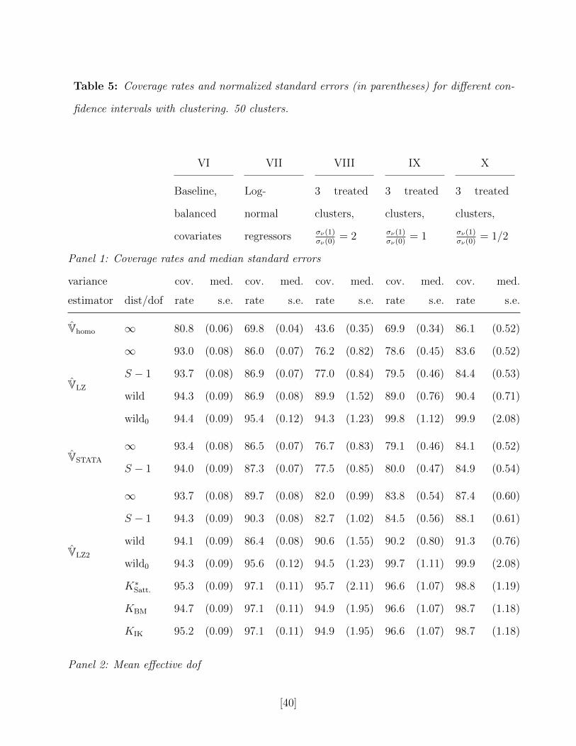
Table 5: Coverage rates and normalized standard errors (in parentheses) for different con-
fidence intervals with clustering. 50 clusters.
VI VII VIII IX X
Baseline,
balanced
covariates
Log-
normal
regressors
3 treated
clusters,
σν(1)σν(0)
= 2
3 treated
clusters,
σν(1)σν(0)
= 1
3 treated
clusters,
σν(1)σν(0)
= 1/2
Panel 1: Coverage rates and median standard errors
variance cov. med. cov. med. cov. med. cov. med. cov. med.
estimator dist/dof rate s.e. rate s.e. rate s.e. rate s.e. rate s.e.
Vhomo ∞ 80.8 (0.06) 69.8 (0.04) 43.6 (0.35) 69.9 (0.34) 86.1 (0.52)
VLZ
∞ 93.0 (0.08) 86.0 (0.07) 76.2 (0.82) 78.6 (0.45) 83.6 (0.52)
S − 1 93.7 (0.08) 86.9 (0.07) 77.0 (0.84) 79.5 (0.46) 84.4 (0.53)
wild 94.3 (0.09) 86.9 (0.08) 89.9 (1.52) 89.0 (0.76) 90.4 (0.71)
wild0 94.4 (0.09) 95.4 (0.12) 94.3 (1.23) 99.8 (1.12) 99.9 (2.08)
VSTATA
∞ 93.4 (0.08) 86.5 (0.07) 76.7 (0.83) 79.1 (0.46) 84.1 (0.52)
S − 1 94.0 (0.09) 87.3 (0.07) 77.5 (0.85) 80.0 (0.47) 84.9 (0.54)
VLZ2
∞ 93.7 (0.08) 89.7 (0.08) 82.0 (0.99) 83.8 (0.54) 87.4 (0.60)
S − 1 94.3 (0.09) 90.3 (0.08) 82.7 (1.02) 84.5 (0.56) 88.1 (0.61)
wild 94.1 (0.09) 86.4 (0.08) 90.6 (1.55) 90.2 (0.80) 91.3 (0.76)
wild0 94.3 (0.09) 95.6 (0.12) 94.5 (1.23) 99.7 (1.11) 99.9 (2.08)
K∗Satt. 95.3 (0.09) 97.1 (0.11) 95.7 (2.11) 96.6 (1.07) 98.8 (1.19)
KBM 94.7 (0.09) 97.1 (0.11) 94.9 (1.95) 96.6 (1.07) 98.7 (1.18)
KIK 95.2 (0.09) 97.1 (0.11) 94.9 (1.95) 96.6 (1.07) 98.7 (1.18)
Panel 2: Mean effective dof
[40]

Table 5: (continued)
K∗Satt. 20 5.4 2.1 2.3 2.2
KBM 28 5.4 2.3 2.3 2.3
KIK 20 5.4 2.3 2.3 2.3
Notes: “cov. rate” refers to coverage of nominal 95% confidence intervals (in percentages),
and “med. s.e.” refers to standard errors normalized by tK0.975/t∞0.975. Variance estimators and
degrees-of-freedom (dof) adjustments are described in the text, wild bootstrap confidence
intervals (“wild” and “wild0”) are described in Appendix A.2. Results are based on 100,000
replications, except for wild wild bootstrap-based confidence intervals, which use 10,000
replications, and 500 bootstrap draws in each replication.
[41]