Robust Shape from Shading

A. G. Jones and C. J. Taylor

Dept. of Medical Biophysics, Stopford Building, University of Manchester, Manchester,

M13 9PT. Phone: 061 275-5130. Fax 061 275-5145

AbstractExisting Shape from Shading algorithms are not robust enough to work reliably with realimages. We present a new paradigm for Shape from Shading based upon & scale space sur-face representation. Using this representation, the Shape from Shading problem becomesone of forming a surface from gaussian basis functions in such a way that the shading in theoriginal image is explained. The algorithm is both fast and robust, producing convincingresults. In its current form, the algorithm requires the reflectance function to be approxi-mately circularly symmetric. We show results for synthetic images, both with and withoutadded noise, and for real Scanning Electron Microscope images.

1 Introduction

Images of three-dimensional objects often show variations in brightness, or shading,across object surfaces, and this information provides an important visual cue for re-covering the shape of an object. Exploiting this information is one of the classic prob-lems of computer vision, known as the shape from shading (SFS) problem [1].

To formulate the problem, we define a three-dimensional Euclidean co-ordinate sys-tem, where the z axis projects directly towards the viewpoint and the x and y axes co-incide with the axes in the image plane. We assume orthographic projection with thelight source at infinity. The visible surface is the function z(x,y), and the surface gradientis the pair (p,q) where p = dz/dx and q = dz/dy , iep and q are the rates of change ofsurface height in the x and y directions respectively. The observed brightness of a sur-face point is directly related to the surface gradient, the position of the light source andthe reflectance properties of the surface. The relationship between the image and thesurface gradient is expressed by the image irradiance equation E(x,y) =R(p,q), where E isthe image, and R is the reflectance function which embodies both the effects of the imag-ing geometry and the reflectance properties of the surface. We assume that the reflec-tance function is of a known analytic form.

The SFS problem is to recover the surface function z(x,y) from the brightness imageE(x,y) by "inverting" the image irradiance equation. Since the problem is undercon-strained, the classical approach has been to introduce a smoothness constraint to regular-ize [1] the problem and thus allow a single solution to be found. The problem is then castas a large non-linear optimisation task, and iterative techniques are used to progressive-ly refine estimates of surface height or gradient. Such algorithms typically suffer anumber of drawbacks:

• Convergence is slow and not robust, especially with noisy data.• The recovered surface gradients may not be integrable (ie they cannot be inte-

grated to form a physically realisable surface).• Algorithm parameters may need careful tuning.

BMVC 1993 doi:10.5244/C.7.15

146

• Boundary conditions are required.• The smoothness constraint can make results overly smooth [1].

In this paper we present a novel scale space [3] SFS algorithm. The algorithm finds par-tial solutions at a range of resolutions, or scales, and combines these to form a completesolution. The approach has a number of advantages:

• Convergence is robust.• No explicit smoothness constraint is required.• The algorithm operates in the space of integrable surfaces, so the solution

surface is always integrable.• No boundary conditions are required.

We show results for synthetic images, both with and without additive noise, and for realScanning Electron Microscope (SEM) images. The SEM imaging process is particularlyappropriate for SFS when the usual assumptions are made, since the projection is ortho-graphic and the "light source" is effectively at infinity.

2 Previous WorkMost Shape from Shading algorithms are based on Horn's formulation, using the Calcu-lus of Variations [6], which involves minimizing an integral equation by solving the asso-ciated Euler equations using an iterative method. The integral equation is typically ofthe form:

J jE(x,y)-R(p,q))2 + l(p\ + p) + q\ + q2y) + fi((zx-pf + (zy-qf) dxdy

where X. and p. are scalar multipliers and the subscripts represent partial differentiation.The first term is the brightness error between the image of the solution surface and theobserved image; the second term is the smoothness (regularization) constraint; and thefinal term penalises departure from integrability. Choosing X and JJL is something of ablack art, with poor choices preventing convergence or creating overly smooth results.Many algorithms first recover surface gradients which are then cast onto the nearestintegrable surface [6][11]. Recently, Horn devised an algorithm that recovers surfaceheight directly, avoiding the problem of ensuring integrability in the gradient field [1].Szeliski [9] improved upon the slow convergence rates of Horn's relaxation schemes byminimising the integral equation directly using conjugate gradient descent [10].Peleg and Ron [8] obtained faster convergence by using a multiresolution approach.Their approach requires the construction of a hierarchy of images of the blurred sur-face, but this cannot be constructed by simply blurring the image itself. They describehow an approximation to the image of the blurred surface can be obtained, and we usethis technique in our algorithm.

Progress has also been made with local algorithms for SFS, most notably the recentwork of Oliensis and Dupuis [2] which casts SFS as an optimal control problem. Theiralgorithm is fast, robust and gives accurate reconstructions, but is unable to cope withinflections and plateaux in the surface and requires prior knowledge about singularpoints (points of zero gradient).

3 Scale Space Shape from ShadingIn this section, we first describe the scale space surface representation, and then de-scribe our SFS algorithm.

147

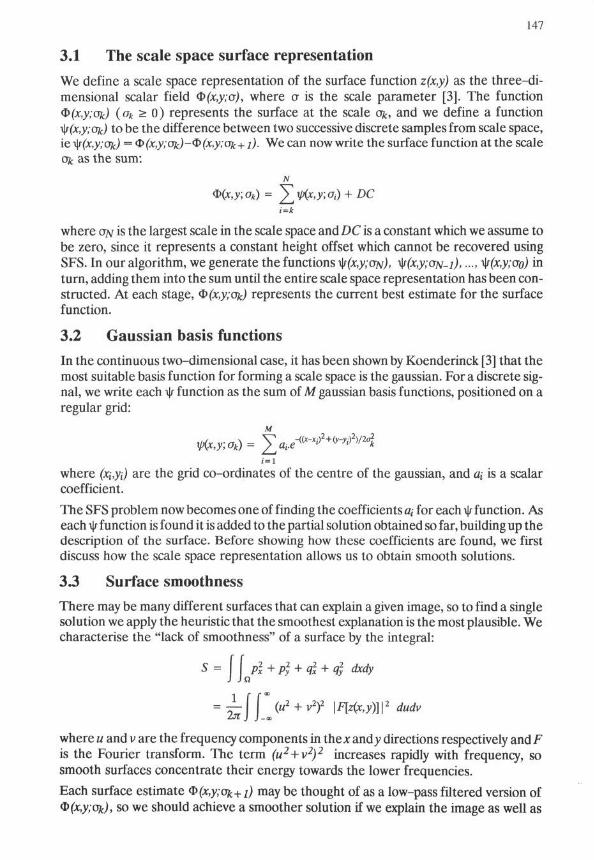
3.1 The scale space surface representation

We define a scale space representation of the surface function z(x,y) as the three-di-mensional scalar field <b(x,y;a), where a is the scale parameter [3]. The function®(x,y;ok) (ok > 0) represents the surface at the scale ofe, and we define a function

to be the difference between two successive discrete samples from scale space,7k) = <b(x,y;ok)-<&(x,y;ak+1). We can now write the surface function at the scale

ofc as the sum:N

Q>(x,y;ok) = Vt/^t,>>;cr,) + DCi=k

where OJV is the largest scale in the scale space and DC is a constant which we assume tobe zero, since it represents a constant height offset which cannot be recovered usingSFS. In our algorithm, we generate the functions ty(x,y;oN), i\r(x,y;aN-2), •••> tyfcyioo) m

turn, adding them into the sum until the entire scale space representation has been con-structed. At each stage, &(x,y;ak) represents the current best estimate for the surfacefunction.

3.2 Gaussian basis functionsIn the continuous two-dimensional case, it has been shown by Koenderinck [3] that themost suitable basis function for forming a scale space is the gaussian. For a discrete sig-nal, we write each i|/ function as the sum of M gaussian basis functions, positioned on aregular grid:

where (xi,yi) are the grid co-ordinates of the centre of the gaussian, and ai is a scalarcoefficient.

The SFS problem now becomes one of finding the coefficients a; for each ty function. Aseach -if function is found it is added to the partial solution obtained so far, building up thedescription of the surface. Before showing how these coefficients are found, we firstdiscuss how the scale space representation allows us to obtain smooth solutions.

3.3 Surface smoothness

There may be many different surfaces that can explain a given image, so to find a singlesolution we apply the heuristic that the smoothest explanation is the most plausible. Wecharacterise the "lack of smoothness" of a surface by the integral:

5 = \\p*+pl + q* + q2y dxdy

("2 + v2)2 I ^ ' ^ I 2 dudv

where u and v are the frequency components in the* andy directions respectively andFis the Fourier transform. The term (u2+v2)2 increases rapidly with frequency, sosmooth surfaces concentrate their energy towards the lower frequencies.

Each surface estimate <&(x,y;ok+i) may be thought of as a low-pass filtered version ofk), so we should achieve a smoother solution if we explain the image as well as

148

possible in $(x,y;ok+i) before moving to the next scale and solving for <&(x,y;ok)- Wetherefore ensure the solution is smooth by finding the \|r functions in the order•ty(x,y;aN), ty(x,y;<TN-i),.... ty(x,y;ao), such that the corresponding surface function alwaysgives a smooth explanation of the image. How we ensure that a smooth surface estimateis found at each scale is described in the next section.

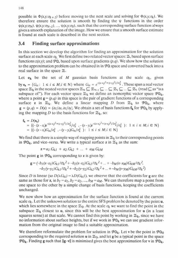
3.4 Finding surface approximations

In this section we develop the algorithm for finding an approximation for the solutionsurface at each scale c%. We first define two related vector spaces: %, based upon surfacefunctions z(x,y); and ^Q, based upon surface gradients (p,q). We show how the solutionto the approximation problem can be obtained in in ^Q. space and converted back into areal surface in the space %.

Let ek be the set of M gaussian basis functions at the scale O&, givenbye* = {Gta: 1 < i < M;i e N} where Gki = g-^V+O1-^2)/^ .These span a real vectorspace 2>k in the nested vector spaces 2>N CZ 2SN-i £ - £ Z>k C ... C 2>0 (read C as "is asubspace of"). For each vector space Z>k we define an isomorphic vector space ^Qk,where a point g = (p,q) in this space is the pair of gradient functions of a correspondingsurface z in Z>^. We define a linear mapping D from 2>k to 90^, whereg = (/>><?) = D(z) - (dz/dx,dz/dy). We obtain a set of basis functions f̂ for SP&k by apply-ing the mapping D to the basis functions for Z>k> so:

fk JD(ek) , , , ,= {(-(x-Xiy«x'x?+(y->-))/2ai/oi ,-(y-yiy

((x^+^)/2i/oi )•. 1 < / < M-I e N}= {(-(x-Xi)Gki/ol ,-(y-ydGkl/a

2k ): 1 < i < M;i E N}

We find that there is a simple way of mapping points in Z^ to their corresponding pointsin ^Qk. and vice-versa. We write a typical surface z in 2->k as the sum:

The point g in 'EPQ.k corresponding to z is given by:

g = (-bi(x-xj)Gkl/Ok2+-b2(x-X2)Gk2/ak

2 + ... +-bM(x-xM)GkM/Ok2,

Since D is linear (so D(\Gid) = kD(Gia)), we observe that the coefficients for g are thesame as those for z, iebi =aj, b2 = a2,..., bu^aM- We can therefore map a point fromone space to the other by a simple change of basis functions, keeping the coefficientsunchanged.

We now show how an approximation for the surface function is found at the currentscale ofc. Let the unknown solution to the entire SFS problem be denoted by the point u,which lies somewhere in the space 2>o- At the scale c% we want to find the point in thesubspace 2Sk closest to u, since this will be the best approximation for u (in a leastsquares sense) at that scale. We cannot find this point by working in 2-ik, since we haveno information about surface heights, but if we work in 9>&k we can use gradient infor-mation from the original image to find a suitable approximation.

We therefore reformulate the problem for solution in <3>Q.^. Let v be the point in ^Qocorresponding to the required solution u in 2Sn, and let g be a typical point in the space

.̂ Finding g such that ||g-v|| is minimised gives the best approximation for v in

149

and hence the best approximation for the solution function u in 2 ^ . Writing g as, and v as (pv,qv), we define the distance between them as the Euclidean norm:

The distance ||g-v|| cannot be measured directly, since v is unknown. However, we canmeasure the brightness error, Q, between the rendered image of g and Ej,, the estimatedimage of a surface formed by blurring v. We find £& by blurring the observed image usingthe algorithm of Ron and Peleg, described in Section 3.6. It is shown in Appendix B thatby minimising Q we can find the surface approximation of maximum likelihood, given theestimated image of the blurred surface, £/,. We define the brightness error as:

Since we know R and £/,, we can use an appropriate optimisation technique to find theset of coefficients for (pg,qg) that minimises Q. Our strategy for finding the next surfaceapproximation <!?(x,y;crk), given that we have already found &(x,y;ok+i), is therefore asfollows:

1. Apply the mapping D to &(x,y;ok+i), expressing the result in terms of thebasis functions f̂ . This is our initial estimate, s, for the best approximationto the solution surface in the space 9*^.

2. From the initial estimate, s, find a function As in 9*0.̂ such that Q(s + As)is a minimum.

3. s + As is expressed in terms of the coefficients a/, G2> •••> aM using the basisfunctions fk- The corresponding surface in Z>k is:

<D(x,y;c%) = ahGkl + a2.Gk2 + aj.G« + ... + aM.GkM

The entire surface description is built up by finding each surface approximation<b(x,y;ak) in turn (for k=N,N-l,... ,1,0), starting from the initial condition <b(x,y;<JN) = 0(ie the first estimate for the surface is a plane). The final solution surface is the function

In Step 2 of the algorithm there may be more than one As that minimises Q, so wechoose the As that gives the smoothest surface. It is shown in Appendix B that the lack-of-smoothness measure Sk for the surface <S}(x,y;ok) is bounded above bySk ^ Sk+l + CII As |p, where Sk+i is the lack-of-smoothness for the previous surface<&(x,y;ok+i) and C is a positive constant. Thus the As of smallest length certainly gives asmooth surface approximation. Since we are sampling scale space densely, the initialestimate s should be close to a minimum in Q, so little more than gradient descent opti-misation should be required to find the minimum in Q of smallest As. To be certain offinding the nearest minimum, the optimisation strategy could be restricted to explorethe region of S'Glk n e a r the initial estimate, but in practice we have found such a restric-tion unnecessary.

3.5 Minimising the brightness errorOur algorithm minimises the brightness error function Q once at each discrete scale, soan efficient optimisation scheme is required. Unfortunately, the brightness error func-

t Here subscripts are for notational purposes and do not denote partial differentiation.

150

tion is difficult to minimise, since it forms a very large non-linear system. We haveadopted a two stage approach, with a Genetic Algorithm (GA) [4] finding a rough esti-mate for the solution, followed by refinement by conjugate gradient descent [10]. The GAconverges rapidly and robustly and is able to cope with plateaux and other anomalies inthe objective function, but does not give an accurate solution. Conjugate gradient de-scent is less robust, but can provide the accuracy required in the final solution, given areasonable starting approximation.

The Genetic AlgorithmThe Genetic Algorithm (GA) is a search algorithm based upon natural genetics and the"survival of the fittest" principle of Darwinian evolution. The GA manipulates apool ofcandidate solutions, each solution being coded as a bit string, or chromosome. Every iter-ation, the GA finds the fitter (ie better) chromosomes in the pool and "breeds" themtogether using genetic operators to form new chromosomes. These new chromosomesform a new pool, replacing the old one. Some of the new chromosomes are likely to befitter than the ones from which they were derived, so there will be net movement to-wards a solution. See [4] for a more detailed description.

The GA owes its efficiency and robustness to a careful balance between exploitation(concentrating effort in promising areas of the search space) and exploration (makingrandom trial moves in the search space). The GA is most suitable for finding good, butnot optimal, solutions to large scale problems. We use the GA to find an initial estimatefor the solution, and it performs well in this role. This estimate is then refined usingconjugate gradient descent.

Conjugate gradient descentConjugate gradient descent is an optimisation technique suitable for solving large, non-linear systems of equations. It uses derivatives to calculate search directions, with eachnew search direction being conjugate to previous search directions - see [10] for a de-tailed discussion of the algorithm.In our application, derivatives are easily computed since the brightness error functioncan be differentiated analytically with respect to the scalar coefficients. The methodperforms well, converging rapidly to a good solution.

3.6 Finding the image of the blurred surfaceWe use the technique of Peleg and Ron [8] to obtain the approximate image of a blurredsurface. This involves blurring the field -Jp2 + a2 derived from the image using the rela-tionship Jp2 + q2 = R~l(E(pc,y)). The technique requires a circularly symmetric reflec-tance function, but we have achieved good results for other reflectance functions, pro-vided that they do not deviate too greatly from the circularly symmetric model.

4 Experimental resultsWe show results for four images: two real SEM images, one of a cylindrical fibre and oneof an electron microscope (EM) grid; and two synthetic images of a hemisphere, onenoiseless and one with 10% additive gaussian noise. Each image is 64 by 64 pixels with256 grey levels. We sampled scale space 32 times. Errors in the recovered height areshown for the synthetic image results, but not for the SEM images since no ground truthwas available for these.

151

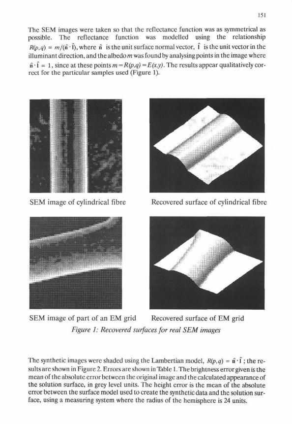
The SEM images were taken so that the reflectance function was as symmetrical aspossible. The reflectance function was modelled using the relationshipR(p,q) = w/(n-f), where n is the unit surface normal vector, f is the unit vector in theilluminant direction, and the albedo m was found by analysing points in the image wheren • I = 1, since at these points m =R(p,q) =E(x,y). The results appear qualitatively cor-rect for the particular samples used (Figure 1).

SEM image of cylindrical fibre Recovered surface of cylindrical fibre

SEM image of part of an EM grid Recovered surface of EM grid

Figure 1: Recovered surfaces for real SEM images

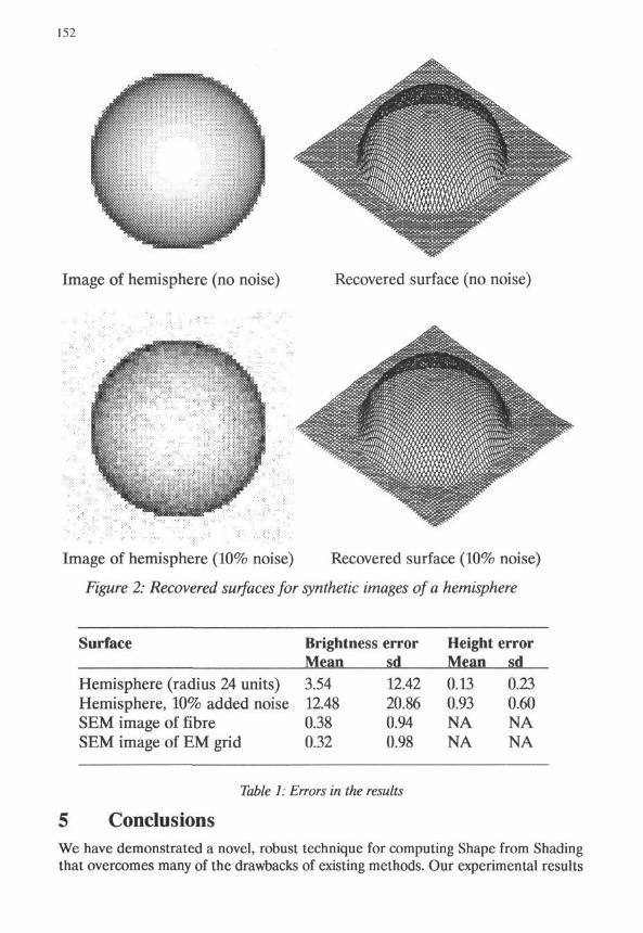
The synthetic images were shaded using the Lambertian model, R(p,q) = n • f; the re-sults are shown in Figure 2. Errors are shown in Table 1. The brightness error given is themean of the absolute error between the original image and the calculated appearance ofthe solution surface, in grey level units. The height error is the mean of the absoluteerror between the surface model used to create the synthetic data and the solution sur-face, using a measuring system where the radius of the hemisphere is 24 units.

152

Image of hemisphere (no noise) Recovered surface (no noise)

Image of hemisphere (10% noise) Recovered surface (10% noise)

Figure 2: Recovered surfaces for synthetic images of a hemisphere

Surface Brightness errorMean sd

Height errorMean sd

Hemisphere (radius 24 units)Hemisphere, 10% added noiseSEM image of fibreSEM image of EM grid

3.5412.480.380.32

12.4220.860.940.98

0.130.93NANA

0.230.60NANA

Table 1: Errors in the results

ConclusionsWe have demonstrated a novel, robust technique for computing Shape from Shadingthat overcomes many of the drawbacks of existing methods. Our experimental results

153

show that the algorithm can produce convincing results rapidly for both synthetic andreal images.

The algorithm constructs a scale space [3] representation of the surface using gaussianbasis functions. This choice of representation incorporates the smoothness assumptionin a natural way, and no explicit smoothness constraint is required. Using this represen-tation, the Shape from Shading problem becomes one of forming a surface from thebasis functions in such a way that the original image is explained. This is done using twooptimisation methods: the Genetic Algorithm [4] and conjugate gradient descent [10].

In future work, we intend to reformulate the problem using a dynamic systemmodel [ 12]. The surface reconstruction will then be created by solving a coupled pair ofdifferential equations using standard numerical techniques. This approach will meanthat we no longer need to solve a new initial value problem at each scale, so it should bemuch more efficient than our current algorithm. We also intend to incorporate stereoinformation into the algorithm in an attempt to improve accuracy and remove some ofthe ambiguity inherent in monocular images.

AcknowledgementsThe author holds a Total Technology studentship funded by SERC and Leica Cambridge Ltd.

Appendix AThe "lack of smoothness" integral for the surface estimate <S>(x,y;Sk) (Ofoy.s*) is represented in9*C!.k by s + As) is given by:

*-!(£)• •(£)'I OS Oi iS | | 2 I, OS Oi \S | | 2

' ax dx " " ay + av "

V 1 ii d s II? II dS ,„ .. 3AS .., ,, 3As ,„ . . , . . . .

Z " ^" +1' ^ H +1' I T H + II17II (tnangle inequality)

xy

aAs

ax " " dy

aAs ||2

a7

N

- JAr+1 + / «; /

1= 1 X^V

—((x—x ) +(v—v") i/^o^

where Gti = e ' ' ** anc | sk+1 is the lack of smoothness of the solution at the previous

scale ok+1. The sum ^ (dG**/axf + (aGfa/^)2 is a positive constant for all; so we denote this

by C and hence write:

This upper bound on the lack of smoothness means that the nearest local minimum in Q (ie the

local minimum of smallest II As | |) is likely to be the smoothest solution at the current scale.

154

Appendix BLet Eb be the approximate image of the blurred solution surface, created by blurring the observedimage using the algorithm of Ron and Peleg (see Section 3.6). For a typical point g in &%,., we useBayes's theorem to write the probability of g given £4 as:

If we assume gaussian noise in the measurement £4, we can obtain:

e(-(Eb-R(pg,qg))2/2s2)

where R is the reflectance function, (pg,qg) = g, and s is the standard deviation of the measurementnoise. We make no prior assumptions so P(g) and P(Ei) are uniform, hence:

2) Eqn. 1

The maximum likelihood (ML) estimate for P(g\Eb) is given by:

gML = argmaxg P{g\Eb)

Taking -fog. of Equation 1, we can write:

gML = argming (Eb-R(pg,qg)f

= argming Q(g)

where Q(g) is the brightness error of the surface g defined in Section 3.4. Our results suggest thatthe quality of the approximation Eb is not critical for the success of the algorithm. The error in theapproximation Eb decreases with scale, and our algorithm seems able to recover from any surfacedistortion this error causes at larger scales. In fact, reasonable results can even be achieved if noblurring is done and the original image is used unchanged.

References[I] Horn, BKP "Height and gradient from shading". AI memo No 1105 May 1989 MIT AI

lab.[2] Dupuis, P and Oliensis, J. "Direct method for reconstructing shape from shading".

IEEE Computer Vision and Pattern Recognition Conf proc, pp453-458, 1992.[3] Koenderinck J.J. Solid Shape. The MIT Press, Cambridge, MA. 1990.[4] Goldberg, David E. Genetic Algorithms in Search, Optimisation and Machine Learning.

Reading, MA. Addison-Wesley, 1988.[5] Forsyth D, Zisserman A. "Shape from Shading in the light of mutual illumination".

Image and Vision Computing. Vol 8 num 1, Feb 1990.[6] Horn, B. K. P. "The Variational Approach to Shape from Shading". CVGIP, Vol. 33, No

2, ppl74-208, February 1986.[7] Burt P.J. "The pyramid as a structure for efficient computation", from Multiresolution

Image Processing and Analysis ed A. Rosenfeld, Springer-Verlag, 1984.[8] Peleg S, Ron G. "Nonlinear multiresolution: A Shape-from-Shading Example". IEEE

PAMI vol 12 num 12, Dec 1990.[9] Szeliski, R. "Fast Shape from Shading". First European conference on Computer Vi-

sion proceedings, Springer-Verlag, 1990.[10] Gill PE, Murray W. Practical optimization. Academic Press, New York, 1981.[II] Chellapa R, Frankot RT. "A method for enforcing integrability in Shape from Shading

algorithms". First Int. Conf. on Computer Vision proceedings, ppll8-127, 1987.[12] Witkin, A, Terzopoulos, D and Kass, M. "Signal matching through scale space". Fifth

Conf. AI proceedings pp714-719, 1986.