Shape and Illumination from Shading using theGeneric Viewpoint Assumption

Daniel Zoran ⇤

CSAIL, MITdanielz@mit.edu

Dilip Krishnan ⇤

CSAIL, MITdilipkay@mit.edu

Jose BentoBoston College

jose.bento@bc.edu

William T. FreemanCSAIL, MIT

billf@mit.edu

Abstract

The Generic Viewpoint Assumption (GVA) states that the position of the vieweror the light in a scene is not special. Thus, any estimated parameters from anobservation should be stable under small perturbations such as object, viewpointor light positions. The GVA has been analyzed and quantified in previous works,but has not been put to practical use in actual vision tasks. In this paper, we showhow to utilize the GVA to estimate shape and illumination from a single shadingimage, without the use of other priors. We propose a novel linearized SphericalHarmonics (SH) shading model which enables us to obtain a computationally ef-ficient form of the GVA term. Together with a data term, we build a model whoseunknowns are shape and SH illumination. The model parameters are estimatedusing the Alternating Direction Method of Multipliers embedded in a multi-scaleestimation framework. In this prior-free framework, we obtain competitive shapeand illumination estimation results under a variety of models and lighting condi-tions, requiring fewer assumptions than competing methods.

1 Introduction

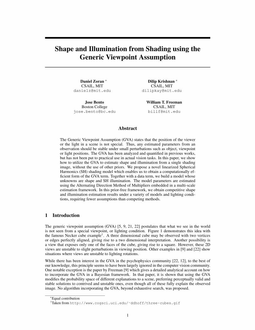
The generic viewpoint assumption (GVA) [5, 9, 21, 22] postulates that what we see in the worldis not seen from a special viewpoint, or lighting condition. Figure 1 demonstrates this idea withthe famous Necker cube example1. A three dimensional cube may be observed with two verticesor edges perfectly aligned, giving rise to a two dimensional interpretation. Another possibility isa view that exposes only one of the faces of the cube, giving rise to a square. However, these 2Dviews are unstable to slight perturbations in viewing position. Other examples in [9] and [22] showsituations where views are unstable to lighting rotations.

While there has been interest in the GVA in the psychophysics community [22, 12], to the best ofour knowledge, this principle seems to have been largely ignored in the computer vision community.One notable exception is the paper by Freeman [9] which gives a detailed analytical account on howto incorporate the GVA in a Bayesian framework. In that paper, it is shown that using the GVAmodifies the probability space of different explanations to a scene, preferring perceptually valid andstable solutions to contrived and unstable ones, even though all of these fully explain the observedimage. No algorithm incorporating the GVA, beyond exhaustive search, was proposed.

⇤Equal contribution1Taken from http://www.cogsci.uci.edu/

˜

ddhoff/three-cubes.gif

1

Figure 1: Illustration of the GVA principle using the Necker cube example. The cube in the middlecan be viewed in multiple ways. However, the views on the left and right require a very specificviewing angle. Slight rotations of the viewer around the exact viewing positions would dramaticallychange the observed image. Thus, these views are unstable to perturbations. The middle view, onthe contrary, is stable to viewer rotations.

Shape from shading is a basic low-level vision task. Given an input shading image - an image ofa constant albedo object depicting only changes in illumination - we wish to infer the shape of theobjects in the image. In other words, we wish to recover the relative depth Z

i

at each pixel i inthe image. Given values of Z, local surface orientations are given by the gradients r

x

Z and ry

Zalong the coordinate axes. A key component in estimating the shape is the illumination L. Theparameters of L may be given with the image, or may need to be estimated from the image alongwith the shape. The latter is a much harder problem due to the ambiguous nature of the problem, asmany different surface orientations and light combinations may explain the same image. While thenotion of a shading image may seem unnatural, extracting them from natural images has been anactive field of research. There are effective ways of decomposing images into shading and albedoimages (so called “intrinsic images” [20, 10, 1, 29]), and the output of those may be used as input toshape from shading algorithms.

In this paper we show how to effectively utilize the GVA for shape and illumination estimation froma single shading image. The only terms in our optimization are the data term which explains theobservation and the GVA term. We propose a novel shading model which is a linearization of thespherical harmonics (SH) shading model [25]. The SH model has been gaining popularity in thevision and graphics communities in recent years [26, 17]) as it is more expressive than the pop-ular single source Lambertian model. Linearizing this model allows us, as we show below, to getsimple expressions for our image and GVA terms, enabling us to use them effectively in an optimiza-tion framework. Given a shading image with an unknown light source, our optimization proceduresolves for the depth and illumination in the scene. We optimize using Alternating Direction Methodof Multipliers (ADMM) [4, 6]. We show that this method is competitive with current shape andillumination from shading algorithms, without the use of other priors over illumination or geometry.

2 Related Work

Classical works on shape from shading include [13, 14, 15, 8, 23] and newer works include [3, 2,19, 30]. It is out of scope of this paper to give a full survey of this well studied field, and we refer thereader to [31] and [28] for good reviews. A large part of the research has been focused on estimatingthe shape under known illumination conditions. While still a hard problem, it is more constrainedthan estimating both the illumination and the shape.

In impressive recent work, Barron and Malik [3] propose a method for estimating not just the illu-mination and shape, but also the albedo of a given masked object from a single image. By usinga number of novel (and carefully balanced) priors over shape (such as smoothness and contour in-formation), albedo and illumination, it is shown that reasonable estimates of shape and illuminationmay be extracted. These priors and the data term are combined in a novel multi-scale frameworkwhich weights coarser scale (lower frequency) estimates of shape more than finer scale estimates.Furthermore, Barron and Malik use a spherical harmonics lighting model to provide for richer re-covery of real world scenes and diffuse outdoor lighting conditions. Another contribution of theirwork has been the observation that joint inference of multiple parameters may prove to be morerobust (although this is hard to prove rigorously). The expansion to the original MIT dataset [11]provided in [3] is also a useful contribution.

2

Another recent notable example is that of Xiong et al. [30]. In this thorough work, the distributionof possible shape/illumination combinations in a small image patch is derived, assuming a quadraticdepth model. It is shown that local patches may be quite informative, and that are only a few possibleexplanations of light/shape pairs for each patch. A framework for estimating full model geometrywith known lighting conditions is also proposed.

3 Using the Generic View Assumption for Shape from Shading

In [9], Freeman gave an analytical framework to use the GVA. However, the computational exam-ples in the paper were restricted to linear shape from shading models. No inference algorithm waspresented; instead the emphasis was on analyzing how the GVA term modifies the posterior dis-tribution of candidate shape and illumination estimates. The key idea in [9] is to marginalize theposterior distribution over a set of “nuisance” parameters - these correspond to object or illumi-nation perturbations. This integration step corresponds to finding a solution that is stable to theseperturbations.

3.1 A Short Introduction to the GVA

Here we give a short summary of the derivations in [9], which we use in our model. We startwith a generative model f for images, which depends on scene parameters Q and a set of genericparameters w. The generative model we use is explained in Section 4. w are the parameters whichwill eventually be marginalized. In our shape and illumination from shading case, f corresponds toour shading model in Eq. 14 (defined below). Q includes both surface depth at each point Z and thelight coefficients vector L. Finally, the generic variable w corresponds to different object rotationangles around different axes of rotations (though there could be other generic variables, we only usethis one). Assuming measurement noise ⌘ the result of the generative process would be:

I = f(Q,w) + ⌘ (1)

Now, given an image I we wish to infer scene parameters Q by marginalizing out the generic vari-ables w. Using Bayes’ theorem, this results in the following probability function:

P (Q|I) = P (Q)

P (I)

Z

wP (w)P (I|Q,w)dw (2)

Assuming a low Gaussian noise model for ⌘, the above integral can be approximated with a Laplaceapproximation, which involves expanding f using a Taylor expansion around w0. We get the fol-lowing expression, aptly named in [9] as the ”scene probability equation”:

P (Q|I) = C|{z}constant

exp

✓�kI� f(Q,w0)k2

2�2

◆

| {z }fidelity

P (Q)P (w0)| {z }prior

1pdetA| {z }

genericity

(3)

where A is a matrix whose i, j-th entry is:

Ai,j

=

@f(Q,w)

@wi

T @f(Q,w)

@wj

(4)

and the derivatives are estimated at w0. A is often called the Fisher information matrix.

Eq. 3 has three terms: the fidelity term (sometimes called the likelihood term, data term or imageterm) tells us how close we are to the observed image. The prior tells us how likely are our currentparameter estimates. The last term, genericity, tells us how much our observed image would changeunder perturbations of the different generic variables. This term is the one which penalizes forunstable results w.r.t to the generic variables. From the form of A, it is clear why the genericity termhelps; the determinant of A is large when the rendered image f changes rapidly with respect to w.This makes the genericity term small and the corresponding hypothesis Q less probable.

3

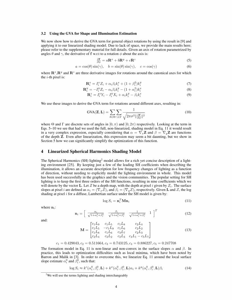
3.2 Using the GVA for Shape and Illumination Estimation

We now show how to derive the GVA term for general object rotations by using the result in [9] andapplying it to our linearized shading model. Due to lack of space, we provide the main results here;please refer to the supplementary material for full details. Given an axis of rotation parametrized byangles ✓ and �, the derivative of f w.r.t to a rotation � about the axis is:

@f@�

= aRx

+ bRy

+ cRz (5)

a = cos(✓) sin(�), b = sin(✓) sin(�), c = cos(�) (6)

where Rx,Ry and Rz are three derivative images for rotations around the canonical axes for whichthe i-th pixel is:

Rx

i

= Ixi

Zi

+ ↵i

�i

kxi

+ (1 + �2i

)kyi

(7)Ry

i

= �Iyi

Zi

� ↵i

�i

kyi

� (1 + ↵2i

)kxi

(8)Rz

i

= Ixi

Yi

� Iyi

Xi

+ ↵i

kyi

� �i

kxi

(9)

We use these images to derive the GVA term for rotations around different axes, resulting in:

GVA(Z,L) =X

✓2⇥

X

�2�

1q2⇡�2k @f

@�

k2(10)

where ⇥ and � are discrete sets of angles in [0,⇡) and [0, 2⇡) respectively. Looking at the term inEqs. 5–10 we see that had we used the full, non-linearized, shading model in Eq. 11 it would resultin a very complex expression, especially considering that ↵ = r

x

Z and � = ry

Z are functionsof the depth Z. Even after linearization, this expression may seem a bit daunting, but we show inSection 5 how we can significantly simplify the optimization of this function.

4 Linearized Spherical Harmonics Shading Model

The Spherical Harmonics (SH) lighting2 model allows for a rich yet concise description of a light-ing environment [25]. By keeping just a few of the leading SH coefficients when describing theillumination, it allows an accurate description for low frequency changes of lighting as a functionof direction, without needing to explicitly model the lighting environment in whole. This modelhas been used successfully in the graphics and the vision communities. The popular setting for SHlighting is to keep the first three orders of the SH functions, resulting in nine coefficients which wewill denote by the vector L. Let Z be a depth map, with the depth at pixel i given by Z

i

. The surfaceslopes at pixel i are defined as ↵

i

= (rx

Z)

i

and �i

= (ry

Z)

i

respectively. Given L and Z, the logshading at pixel i for a diffuse, Lambertian surface under the SH model is given by:

logSi

= nT

i

Mni

(11)

where ni

:

ni

=

h↵ip

1+↵

2i+�

2i

�ip1+↵

2i+�

2i

1p1+↵

2i+�

2i

1

iT

(12)

and:

M =

2

64

c1L9 c1L5 c1L8 c2L4

c1L5 �c1L9 c1L6 c2L2

c1L8 c1L6 c3L7 c2L3

c2L4 c2L2 c2L3 c4L1 � c5L7

3

75 (13)

c1 = 0.429043, c2 = 0.511664, c3 = 0.743125, c4 = 0.886227, c5 = 0.247708

The formation model in Eq. 11 is non-linear and non-convex in the surface slopes ↵ and �. Inpractice, this leads to optimization difficulties such as local minima, which have been noted byBarron and Malik in [3]. In order to overcome this, we linearize Eq. 11 around the local surfaceslope estimate ↵0

i

and �0i

, such that:

logSi

⇡ kc(↵0i

,�0i

,L) + kx(↵0i

,�0i

,L)↵i

+ ky(↵0i

,�0i

,L)�i

(14)2We will use the terms lighting and shading interchangeably

4

where the local surface slopes are estimated in a local patch around each pixel in our current esti-mated surface. The derivation of the linearization is given in the supplementary material. For thesake of brevity, we will omit the dependence on the ↵0

i

,�0i

and L terms, and denote the coefficientsat each location as kc

i

,kxi

and kyi

respectively for the remainder of the paper.

A natural question is the accuracy of the linearized model Eq. 14. The linearization is accuratein most situations where the depth Z changes gradually, such that the change in slope is linear orsmall in magnitude. In [30], locally quadratic shapes are assumed; this leads to linear changes inslopes, and in such situations, the linearization is highly accurate. We tested the accuracy of thelinearization by computing the difference between the estimates in Eq. 14 and Eq. 11, over groundtruth shape and illumination estimates. We found it to be highly accurate for the models in ourexperiments. The linearization in Eq. 14 leads to a quadratic formation model for the image term(described in Section 5.2.1), leading to more efficient updates for ↵ and �. Furthermore, this allowsus to effectively incorporate the GVA even with the spherical harmonics framework.

5 Optimization using the Alternating Direction Method of Multipliers

5.1 The Cost Function

Following Eq. 3, we can now derive the cost function we will optimize w.r.t the scene parametersZ and L. To derive a MAP estimate, we take the negative log of Eq. 3 and use constant priors overboth the scene parameters and the generic variables; thus we have a prior-free cost function. Thisresults in the following cost:

g(Z,L) = �imgkI� logS(Z,L)k2 � �GVA logGVA(Z,L) (15)where f(Z,L) = logS(Z,L) is our linearized shading model Eq. 14 and the GVA term is defined inEq. 10. �img and �GVA are hyper-parameters which we set to 2 and 1 respectively for all experiments.Because of the dependence of ↵ and � on Z directly optimizing for this cost function is hard, as itresults in a large, non-linear differential system for Z. In order to make this more tractable, weintroduce ↵ and ˜�, the surface spatial derivatives, as auxiliary variables, and solve for the followingcost function which constrains the resulting surface to be integrable:

g(Z, ↵, ˜�,L|I) = �imgkI� logS(↵, ˜�,L)k2 � �GVA logGVA(Z, ↵, ˜�,L) (16)

s.t ↵ = rx

Z, ˜� = ry

Z, ry

rx

Z = rx

ry

Z

ADMM allows us to subdivide the cost into relatively simple subproblems, solve each one indepen-dently and then aggregate the results. We briefly review the message passing variant of ADMM [7]in the supplementary material.

5.2 Subproblems

5.2.1 Image Term

This subproblem ties our solution to the input log shading image. The participating variables are theslopes ↵ and ˜� and illumination L. We minimize the following cost:

argmin

↵,�,L

�imgX

i

⇣Ii

� kci

� kxi

↵i

� kyi

˜�i

⌘2+

⇢

2

k↵� n↵

k2 + ⇢

2

k˜� � n�

k2 + ⇢

2

kL� nLk2 (17)

where n↵

, n�

and nL are the incoming messages for the corresponding variables as described above.We solve this subproblem iteratively: for ↵ and ˜� we keep L constant (and as a result the k-s areconstant). A closed form solution exists since this is just a quadratic due to our relinearization model.In order to solve for L we do a few (5 to 10) steps of L-BFGS [27].

5.2.2 GVA Term

The participating variables here are the depth values Z, the slopes ↵ and ˜� and the light L. We lookfor the parameters which minimize:

argmin

Z,↵,�,L

� �GVA

2

logGVA(Z, ↵, ˜�,L) +⇢

2

k↵� n↵

k2 + ⇢

2

k˜� � n�

k2 + ⇢

2

kL� nLk2 (18)

5

Here, though the expression for the GVA (Eq. 10) term is greatly simplified due to the shading modellinearization, we have to resort to numerical optimization. We solve for the parameters using a fewsteps of L-BFGS [27].

5.2.3 Depth Integrability Constraint

Shading only depends on local slope (regardless of the choice of shading model, as long as thereare no shadows in the scene), hence the image term only gives us information about surface slopes.Using this information we need to find an integrable surface Z [8]. Finding integrable surfaces fromlocal slope measurements has been a long standing research question and there are several waysof doing this [8, 14, 18]. By finding such as a surface we will satisfy both constraints in Eq. 16automatically. Enforcing integrability through message passing was performed in [24], where it wasshown to be helpful in recovering smooth surfaces. In that work, belief propagation based message-passing was used. The cost for this subproblem is:

argmin

Z,↵,�

⇢

2

kZ� nZk2 +⇢

2

k↵� n↵

k2 + ⇢

2

k˜� � n�

k2 (19)

s.t ↵ = rx

Z, ˜� = ry

Z, ry

rx

Z = rx

ry

Z

We solve for the surface Z given the messages for the slopes n↵

and n�

by solving a least squaressystem to get the integrable surface. Then, the solution for ↵ and ˜� is just the spatial derivative ofthe resulting surface, satisfying all the constraints and minimizing the cost simultaneously.

5.3 Relinearization

After each ADMM iteration, we perform re-linearization of the kc

,kx

and ky

coefficients. We takethe current estimates for Z and L and use them as input to our linearization procedure (see thesupplementary material for details). These coefficients are then used for the next ADMM iteration.and this process is repeated.

6 Experiments and Results

����� ������

�

��

��

� �������� �������� ��� ���

(a) Models from [30] using“lab” lights

����� ������

�

��

��

�

��

��

���������� �������� ��� ���

(b) MIT models using“natural” lights

����� ������

�

��

��

�

��

��

���������� �������� ��� ���

(c) Average result over allmodels and lights

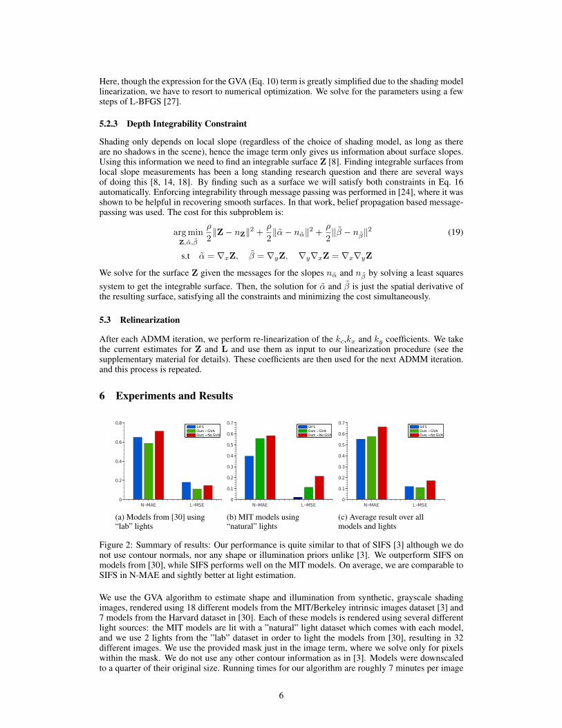
Figure 2: Summary of results: Our performance is quite similar to that of SIFS [3] although we donot use contour normals, nor any shape or illumination priors unlike [3]. We outperform SIFS onmodels from [30], while SIFS performs well on the MIT models. On average, we are comparable toSIFS in N-MAE and sightly better at light estimation.

We use the GVA algorithm to estimate shape and illumination from synthetic, grayscale shadingimages, rendered using 18 different models from the MIT/Berkeley intrinsic images dataset [3] and7 models from the Harvard dataset in [30]. Each of these models is rendered using several differentlight sources: the MIT models are lit with a ”natural” light dataset which comes with each model,and we use 2 lights from the ”lab” dataset in order to light the models from [30], resulting in 32different images. We use the provided mask just in the image term, where we solve only for pixelswithin the mask. We do not use any other contour information as in [3]. Models were downscaledto a quarter of their original size. Running times for our algorithm are roughly 7 minutes per image

6

Gro

und

Trut

hO

urs

-GVA

SIFS

Our

s-N

oG

VA

Viewpoint 1 Viewpoint 2 Estimated Light Rendered Image

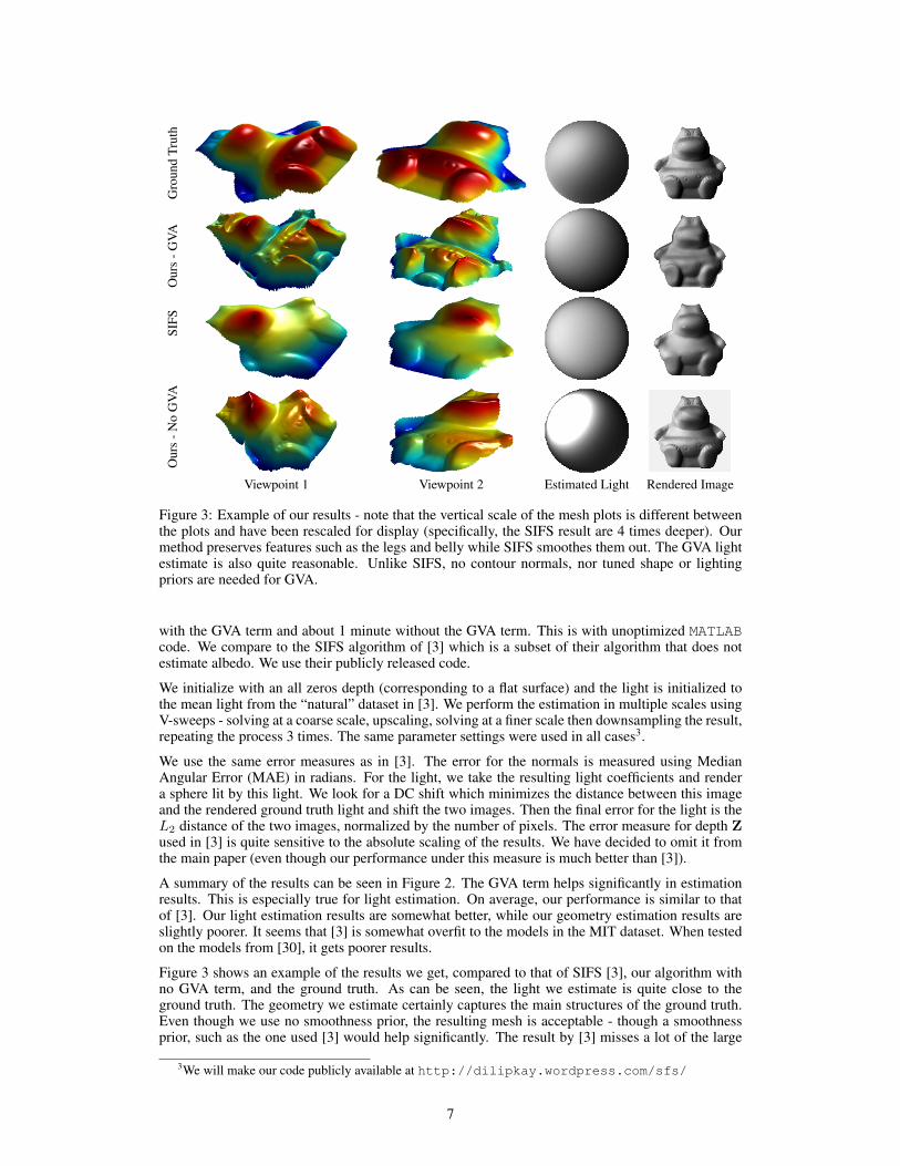
Figure 3: Example of our results - note that the vertical scale of the mesh plots is different betweenthe plots and have been rescaled for display (specifically, the SIFS result are 4 times deeper). Ourmethod preserves features such as the legs and belly while SIFS smoothes them out. The GVA lightestimate is also quite reasonable. Unlike SIFS, no contour normals, nor tuned shape or lightingpriors are needed for GVA.

with the GVA term and about 1 minute without the GVA term. This is with unoptimized MATLABcode. We compare to the SIFS algorithm of [3] which is a subset of their algorithm that does notestimate albedo. We use their publicly released code.

We initialize with an all zeros depth (corresponding to a flat surface) and the light is initialized tothe mean light from the “natural” dataset in [3]. We perform the estimation in multiple scales usingV-sweeps - solving at a coarse scale, upscaling, solving at a finer scale then downsampling the result,repeating the process 3 times. The same parameter settings were used in all cases3.

We use the same error measures as in [3]. The error for the normals is measured using MedianAngular Error (MAE) in radians. For the light, we take the resulting light coefficients and rendera sphere lit by this light. We look for a DC shift which minimizes the distance between this imageand the rendered ground truth light and shift the two images. Then the final error for the light is theL2 distance of the two images, normalized by the number of pixels. The error measure for depth Zused in [3] is quite sensitive to the absolute scaling of the results. We have decided to omit it fromthe main paper (even though our performance under this measure is much better than [3]).

A summary of the results can be seen in Figure 2. The GVA term helps significantly in estimationresults. This is especially true for light estimation. On average, our performance is similar to thatof [3]. Our light estimation results are somewhat better, while our geometry estimation results areslightly poorer. It seems that [3] is somewhat overfit to the models in the MIT dataset. When testedon the models from [30], it gets poorer results.

Figure 3 shows an example of the results we get, compared to that of SIFS [3], our algorithm withno GVA term, and the ground truth. As can be seen, the light we estimate is quite close to theground truth. The geometry we estimate certainly captures the main structures of the ground truth.Even though we use no smoothness prior, the resulting mesh is acceptable - though a smoothnessprior, such as the one used [3] would help significantly. The result by [3] misses a lot of the large

3We will make our code publicly available at http://dilipkay.wordpress.com/sfs/

7

Gro

und

Trut

hO

urs

-GVA

SIFS

Our

s-N

oG

VA

Viewpoint 1 Viewpoint 2 Estimated Light Rendered Image

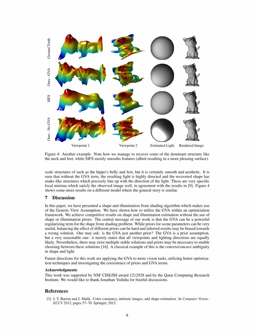
Figure 4: Another example. Note how we manage to recover some of the dominant structure likethe neck and feet, while SIFS mostly smooths features (albeit resulting in a more pleasing surface).

scale structures of such as the hippo’s belly and feet, but it is certainly smooth and aesthetic. It isseen that without the GVA term, the resulting light is highly directed and the recovered shape hassnake-like structures which precisely line up with the direction of the light. These are very specificlocal minima which satisfy the observed image well, in agreement with the results in [9]. Figure 4shows some more results on a different model where the general story is similar.

7 DiscussionIn this paper, we have presented a shape and illumination from shading algorithm which makes useof the Generic View Assumption. We have shown how to utilize the GVA within an optimizationframework. We achieve competitive results on shape and illumination estimation without the use ofshape or illumination priors. The central message of our work is that the GVA can be a powerfulregularizing term for the shape from shading problem. While priors for scene parameters can be veryuseful, balancing the effect of different priors can be hard and inferred results may be biased towardsa wrong solution. One may ask: is the GVA just another prior? The GVA is a prior assumption,but a very reasonable one: it merely states that all viewpoints and lighting directions are equallylikely. Nevertheless, there may exist multiple stable solutions and priors may be necessary to enablechoosing between these solutions [16]. A classical example of this is the convex/concave ambiguityin shape and light.

Future directions for this work are applying the GVA to more vision tasks, utilizing better optimiza-tion techniques and investigating the coexistence of priors and GVA terms.

AcknowledgmentsThis work was supported by NSF CISE/IIS award 1212928 and by the Qatar Computing ResearchInstitute. We would like to thank Jonathan Yedidia for fruitful discussions.

References[1] J. T. Barron and J. Malik. Color constancy, intrinsic images, and shape estimation. In Computer Vision–

ECCV 2012, pages 57–70. Springer, 2012.

8

[2] J. T. Barron and J. Malik. Shape, albedo, and illumination from a single image of an unknown object.In Computer Vision and Pattern Recognition (CVPR), 2012 IEEE Conference on, pages 334–341. IEEE,2012.

[3] J. T. Barron and J. Malik. Shape, illumination, and reflectance from shading. Technical ReportUCB/EECS-2013-117, EECS, UC Berkeley, May 2013.

[4] J. Bento, N. Derbinsky, J. Alonso-Mora, and J. S. Yedidia. A message-passing algorithm for multi-agenttrajectory planning. In Advances in Neural Information Processing Systems, pages 521–529, 2013.

[5] T. O. Binford. Inferring surfaces from images. Artificial Intelligence, 17(1):205–244, 1981.[6] S. Boyd, N. Parikh, E. Chu, B. Peleato, and J. Eckstein. Distributed optimization and statistical learning

via the alternating direction method of multipliers. Foundations and Trends R� in Machine Learning,3(1):1–122, 2011.

[7] N. Derbinsky, J. Bento, V. Elser, and J. S. Yedidia. An improved three-weight message-passing algorithm.arXiv preprint arXiv:1305.1961, 2013.

[8] R. T. Frankot and R. Chellappa. A method for enforcing integrability in shape from shading algorithms.Pattern Analysis and Machine Intelligence, IEEE Transactions on, 10(4):439–451, 1988.

[9] W. T. Freeman. Exploiting the generic viewpoint assumption. International Journal of Computer Vision,20(3):243–261, 1996.

[10] P. V. Gehler, C. Rother, M. Kiefel, L. Zhang, and B. Scholkopf. Recovering intrinsic images with a globalsparsity prior on reflectance. In NIPS, volume 2, page 4, 2011.

[11] R. Grosse, M. K. Johnson, E. H. Adelson, and W. T. Freeman. Ground truth dataset and baseline evalu-ations for intrinsic image algorithms. In Computer Vision, 2009 IEEE 12th International Conference on,pages 2335–2342. IEEE, 2009.

[12] D. D. Hoffman. Genericity in spatial vision. Geometric Representations of Perceptual Phenomena:Papers in Honor of Tarow indow on His 70th Birthday, page 95, 2013.

[13] B. K. Horn. Obtaining shape from shading information. MIT press, 1989.[14] B. K. Horn and M. J. Brooks. The variational approach to shape from shading. Computer Vision, Graph-

ics, and Image Processing, 33(2):174–208, 1986.[15] K. Ikeuchi and B. K. Horn. Numerical shape from shading and occluding boundaries. Artificial intelli-

gence, 17(1):141–184, 1981.[16] A. D. Jepson. Comparing stories. Perception as Bayesian Inference, pages 478–488, 1995.[17] J. Kautz, P.-P. Sloan, and J. Snyder. Fast, arbitrary brdf shading for low-frequency lighting using spherical

harmonics. In Proceedings of the 13th Eurographics workshop on Rendering, pages 291–296. Eurograph-ics Association, 2002.

[18] P. Kovesi. Shapelets correlated with surface normals produce surfaces. In Computer Vision, 2005. ICCV2005. Tenth IEEE International Conference on, volume 2, pages 994–1001. IEEE, 2005.

[19] B. Kunsberg and S. W. Zucker. The differential geometry of shape from shading: Biology reveals curva-ture structure. In Computer Vision and Pattern Recognition Workshops (CVPRW), 2012 IEEE ComputerSociety Conference on, pages 39–46. IEEE, 2012.

[20] Y. Li and M. S. Brown. Single image layer separation using relative smoothness. CVPR, 2014.[21] J. Malik. Interpreting line drawings of curved objects. International Journal of Computer Vision, 1(1):73–

103, 1987.[22] K. Nakayama and S. Shimojo. Experiencing and perceiving visual surfaces. Science, 257(5075):1357–

1363, 1992.[23] A. P. Pentland. Linear shape from shading. International Journal of Computer Vision, 4(2):153–162,

1990.[24] N. Petrovic, I. Cohen, B. J. Frey, R. Koetter, and T. S. Huang. Enforcing integrability for surface re-

construction algorithms using belief propagation in graphical models. In Computer Vision and PatternRecognition, 2001. CVPR 2001. Proceedings of the 2001 IEEE Computer Society Conference on, vol-ume 1, pages I–743. IEEE, 2001.

[25] R. Ramamoorthi and P. Hanrahan. An efficient representation for irradiance environment maps. In Pro-ceedings of the 28th annual conference on Computer graphics and interactive techniques, pages 497–500.ACM, 2001.

[26] R. Ramamoorthi and P. Hanrahan. A signal-processing framework for inverse rendering. In Proceedingsof the 28th annual conference on Computer graphics and interactive techniques, pages 117–128. ACM,2001.

[27] M. Schmidt. Minfunc, 2005.[28] R. Szeliski. Computer vision: algorithms and applications. Springer, 2010.[29] Y. Weiss. Deriving intrinsic images from image sequences. In Computer Vision, 2001. ICCV 2001.

Proceedings. Eighth IEEE International Conference on, volume 2, pages 68–75. IEEE, 2001.[30] Y. Xiong, A. Chakrabarti, R. Basri, S. J. Gortler, D. W. Jacobs, and T. Zickler. From shading to local

shape. http://arxiv.org/abs/1310.2916, 2014.[31] R. Zhang, P.-S. Tsai, J. E. Cryer, and M. Shah. Shape-from-shading: a survey. Pattern Analysis and

Machine Intelligence, IEEE Transactions on, 21(8):690–706, 1999.

9

Shape and Illumination From Shading Using the

Generic Viewpoint Assumption - Supplementary

Material

Daniel Zoran

⇤

CSAIL, MITdanielz@mit.edu

Dilip Krishnan

⇤

CSAIL, MITdilipkay@mit.edu

Jose Bento

Boston Collegejose.bento@bc.edu

William T. Freeman

CSAIL, MITbillf@mit.edu

In this supplementary material, we provide various technical details for our paper. The latest copyof the paper and this supplementary material will be available on the project webpage http://dilipkay.wordpress.com/sfs/.

1 Depth Error Measure

In Table 1, we show the errors between ground truth depth and our depth measurements usingthe Z-MAE error measure introduced in [1]. It can be seen that our algorithms have consistentlylower error. However, this error measure is highly dependent on the absolute range of values in therecovered depth Z. The error measure is not consistent with perceptual assessment of recovereddepth quality, and so we report it here only for completeness.

Method Natural Lights Lab Lights All LightsSIFS 11.5 10.7 11.3

Ours - GVA 8.3 6.0 7.8Ours - no GVA 8.4 6.2 7.9

Table 1: Median Error of recovered depth values (called Z-MAE in [1]).

2 Derivation of Linearization Formula

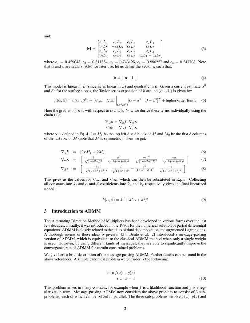
As shown in our paper, the effectiveness of using GVA in a computational framework relies heavilyon the relinearization of the Spherical Harmonics lighting model. The original non-linear modelthat generates the log shading pixels is given by the following per-pixel equation (each pixel isindependent of the others):

h(↵,�) = n

T

Mn (1)

where n is given by:

n =h

↵p1+↵

2+�

2

�p1+↵

2+�

2

1p1+↵

2+�

21i

(2)

⇤Equal contribution

1

and:

M =

2

64

c1L9 c1L5 c1L8 c2L4

c1L5 �c1L9 c1L6 c2L2

c1L8 c1L6 c3L7 c2L3

c2L4 c2L2 c2L3 c4L1 � c5L7

3

75 (3)

where c1 = 0.429043, c2 = 0.511664, c3 = 0.743125, c4 = 0.886227 and c5 = 0.247708. Notethat ↵ and � are scalars. Also for later use, let us define the vector x such that:

n = [ x 1 ] (4)

This model is linear in L (since M is linear in L) and quadratic in n. Given a current estimate ↵

0

and �

0 for the surface slopes, the Taylor series expansion of h around (↵0,�0) is given by:

h(↵,�) = h(↵0,�

0) + [r↵

h r�

h]

����(↵0

,�

0)

[↵� ↵

0� � �

0]T + higher order terms (5)

Here the gradient of h is with respect to ↵ and �. Now we derive these terms individually using thechain rule:

r↵

h = rx

f r↵

x

r�

h = rx

f r�

x

where x is defined in Eq. 4. Let M1 be the top left 3⇥ 3 block of M and M2 be the first 3 columnsof the last row of M (note that M is symmetric). Then we get:

rx

h = [2xM1 + 2M2] (6)

r↵

x =h

1p1+↵

2+�

2� ↵

2p(1+↵

2+�

2)3�↵�p

(1+↵

2+�

2)3�↵p

(1+↵

2+�

2)3

i(7)

r�

x =h

�↵�p(1+↵

2+�

2)31p

1+↵

2+�

2� �

2

(1+↵

2+�

2)3��p

(1+↵

2+�

2)3

i(8)

This gives us the values for r↵

h and r�

h, which can then be substituted in Eq. 5. Collectingall constants into k

c

and ↵ and � coefficients into k

x

and k

y

respectively gives the final linearizedmodel:

h(↵,�) ⇡ k

c + k

x

↵+ k

y

� (9)

3 Introduction to ADMM

The Alternating Direction Method of Multipliers has been developed in various forms over the lastfew decades. Initially, it was introduced in the 1970s for the numerical solution of partial differentialequations. ADMM is closely related to the ideas of dual decomposition and augmented Lagrangians.A thorough review of these ideas is given in [3]. Bento et al. [2] introduced a message-passingversion of ADMM, which is equivalent to the classical ADMM method when only a single weightis used. However, by using different kinds of messages, they are able to significantly improve theconvergence rate of ADMM for certain constrained problems.

We give here a brief description of the message passing ADMM. Further details can be found in theabove references. A simple canonical problem we consider is the following:

min f(x) + g(z)

s.t. x = z (10)

This problem arises in many contexts, for example when f is a likelihood function and g is a reg-ularization term. Message-passing ADMM now considers the above problem to consist of 3 sub-problems, each of which can be solved in parallel. The three sub-problems involve f(x), g(z) and

2

the constraint x = z respectively. Thus the variable x is involved in 2 sub-problems, and the vari-able z in two sub-problems. There are two conflicting requirements to ensure that we make progress:each sub-problem must make progress towards minimizing it’s own cost function; and secondly, itmust not provide a solution that is completely different from the other sub-problem that involves thesame variables.

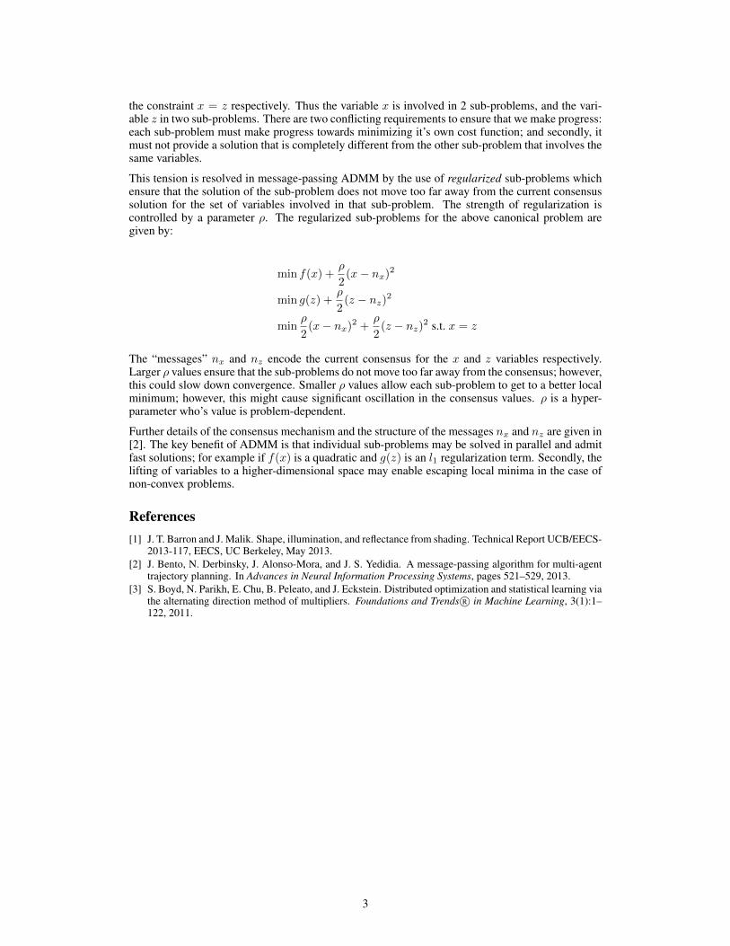
This tension is resolved in message-passing ADMM by the use of regularized sub-problems whichensure that the solution of the sub-problem does not move too far away from the current consensussolution for the set of variables involved in that sub-problem. The strength of regularization iscontrolled by a parameter ⇢. The regularized sub-problems for the above canonical problem aregiven by:

min f(x) +⇢

2(x� n

x

)2

min g(z) +⇢

2(z � n

z

)2

min⇢

2(x� n

x

)2 +⇢

2(z � n

z

)2 s.t. x = z

The “messages” n

x

and n

z

encode the current consensus for the x and z variables respectively.Larger ⇢ values ensure that the sub-problems do not move too far away from the consensus; however,this could slow down convergence. Smaller ⇢ values allow each sub-problem to get to a better localminimum; however, this might cause significant oscillation in the consensus values. ⇢ is a hyper-parameter who’s value is problem-dependent.

Further details of the consensus mechanism and the structure of the messages nx

and n

z

are given in[2]. The key benefit of ADMM is that individual sub-problems may be solved in parallel and admitfast solutions; for example if f(x) is a quadratic and g(z) is an l1 regularization term. Secondly, thelifting of variables to a higher-dimensional space may enable escaping local minima in the case ofnon-convex problems.

References

[1] J. T. Barron and J. Malik. Shape, illumination, and reflectance from shading. Technical Report UCB/EECS-2013-117, EECS, UC Berkeley, May 2013.

[2] J. Bento, N. Derbinsky, J. Alonso-Mora, and J. S. Yedidia. A message-passing algorithm for multi-agenttrajectory planning. In Advances in Neural Information Processing Systems, pages 521–529, 2013.

[3] S. Boyd, N. Parikh, E. Chu, B. Peleato, and J. Eckstein. Distributed optimization and statistical learning viathe alternating direction method of multipliers. Foundations and Trends

R� in Machine Learning, 3(1):1–122, 2011.

3