Robust FEM-based extractionof finite-time coherent sets using

scattered, sparse, and incomplete trajectories

Gary Froyland Oliver Junge

May 4, 2017

Abstract

Transport and mixing properties of aperiodic flows are crucial to a dynamical anal-ysis of the flow, and often have to be carried out with limited information. Finite-timecoherent sets are regions of the flow that minimally mix with the remainder of theflow domain over the finite period of time considered. In the purely advective settingthis is equivalent to identifying sets whose boundary interfaces remain small through-out their finite-time evolution. Finite-time coherent sets thus provide a skeleton ofdistinct regions around which more turbulent flow occurs. They manifest in geophys-ical systems in the forms of e.g. ocean eddies, ocean gyres, and atmospheric vortices.In real-world settings, often observational data is scattered and sparse, which makesthe difficult problem of coherent set identification and tracking even more challeng-ing. We develop three FEM-based numerical methods to efficiently approximate thedynamic Laplace operator, and rapidly and reliably extract finite-time coherent setsfrom models or scattered, possibly sparse, and possibly incomplete observed data.

1 Introduction

The quantification of transport and mixing processes in nonlinear dynamical systems is keyto understanding their global dynamics. In the autonomous setting, where the governingdynamical laws do not change over time, stable and unstable manifolds of low-period orbitshave been used to describe the global dynamics. For example, co-dimension 1 invariantmanifolds represent an impenetrable barrier to trajectories. In the case of periodically-forced flows, the intersections of stable and unstable manifolds form mobile parcels dubbed“lobes”, which give rise to lobe dynamics [26, 30] as a mechanism for transport acrossperiodically varying invariant manifolds.

In the autonomous setting, the concept of almost-invariant sets, introduced in [8] andfurther developed in [15, 12] uses the transfer (or Perron-Frobenius) operator to find regionsin phase space which are either invariant, or in the absence of any open invariant sets, asclose to invariant as possible. Such sets decompose the phase space into regions whichare as dynamically disconnected as possible, and between which transport is minimized.

1

Related approaches to finding “ergodic partitions” in phase space have also been developedusing long orbits [28] or using the Koopman operator [4], the dual of the transfer operator.

In the case of nonautonomous, aperiodic dynamics, the notion of almost-invariant setswas generalized to coherent sets [18] and shortly thereafter to finite-time coherent sets[20, 13]. While almost-invariant sets remain fixed in phase space, when the underlyinggoverning dynamics is time-varying, it is essential to allow sets that are parameterised bytime. Nevertheless, the underlying idea, minimising mixing with the surrounding phasespace, is common to both almost-invariant and finite-time coherent sets. As in the caseof almost-invariant sets, one numerically constructs a transfer operator for the duration ofthe dynamics to be considered. This transfer operator will push forward densities over thechosen time interval. After some straightforward normalising procedures, one computesthe subdominant singular spectrum and singular vectors of the transfer operator, whichindicate the presence and location of finite-time coherent sets. This construction relies ona small amount of diffusion being present in the dynamics; this diffusion can be part ofthe model, or if the underlying dynamics is purely advective it can be easily numericallyinduced.

An equivalent definition of finite-time coherent sets was introduced in [14], specificallyaimed at the case of purely advective dynamics. The underlying goal is to determineco-dimension 1 manifolds whose size remains small relative to enclosed1 volume, underevolution by the dynamics. This idea extends the classical (static) isoperimetric prob-lem [3] of determining the co-dimension 1 manifold with least size given a fixed enclosedvolume. The idea to define finite-time coherent sets as those sets with boundaries thathave dynamically minimal size relative to enclosed volume is consistent with the minimalL2-mixing approach of [13] because if small-amplitude diffusion is added, L2 mixing canonly occur along the boundary interfaces between coherent regions. This fact has beenformally established in [14] in the volume-preserving setting and [17] in the non-volume-preserving case. The persistently minimal size of the boundary of finite-time coherent setsin this sense is also broadly consistent with the approach of [24]. Related work [25] usesa time-dependent metric induced by the advective flow in order to define coherent sets asalmost-invariant sets in the material manifold and thus conceptually separates diffusionfrom advection. In approximating the time dependent metric by a single one they end upwith a similar operator as the dynamic Laplacian in [14, 17].

Numerical implementation of the method of [14] requires approximation of eigenfunc-tions of a dynamic Laplace operator, which consists of the Laplace operator composed withtransfer operators, or equivalently, combinations of Laplace-Beltrami operators with re-spect to Riemannian metrics pulled back under the nonlinear dynamics [25]. The papers[14, 17] used low-order methods such as finite-difference to approximate the Laplace oper-ator and Ulam’s method [35] to approximate the transfer operators. In [16], the authorsinvestigated the use of radial basis functions (RBFs) as an approximating basis for L2,seeking to exploit the smoothness of the underlying dynamics to achieve accurate resultswith relatively sparse trajectory information. This approach successfully achieved very ac-curate results with relatively sparse data, but due to known issues with RBF interpolation

1The boundary of the domain may take part in the enclosing.

2

[37, 11] care must be taken when selecting the RBF centre spacing and RBF radii. Anatural choice of RBF centres would be trajectory points and thus for irregularly scatteredtrajectories, this choice is not always a good one.

On the other hand, the dynamic Laplacian is a self-adjoint, elliptic differential operatorand arguably the finite element method (FEM) is the standard numerical method to dis-cretize these. In fact, also in our specific context, there are a number of major advantagesto this method:

• Sparsity: We obtain a sparse discrete problem. Thus, the computational cost growsonly linearly with the number of mesh elements and enables to use high resolutionmeshes (in contrast to the RBF approach [16]).

• Structure preservation: The dynamic Laplacian is self-adjoint and thus its weak formis symmetric. This symmetry is inherited in the discrete eigenproblem, ensuring apurely real spectrum.

• Arbitrary domains: FEMs can handle arbitrarily shaped domains, as often occur inapplications, unlike spectral methods, which require periodic domains.

• Natural boundary conditions: Homogeneous Neumann boundary conditions are thenatural ones in our context and completely disappear in the weak formulation. Ho-mogeneous Dirichlet conditions can also easily be incorporated.

• Error estimates: There is a standard convergence theory for FEM approximation ofelliptic eigenproblems which directly applies here.

We would further like to highlight advantages over other existing methods for extracting(finite time) coherent sets:

1. There is no free parameter to choose (like a cut-off radius, a neighborhood sizeetc.) experimentally or heuristically when computing the eigenvectors. When ex-tracting coherent sets from these, some heuristics may need to enter in choosing howmany/which eigenvectors yield relevant information. In many cases, this choice issupported by an eigengap heuristic.

2. Even in the case of scattered and sparse trajectory data, we always obtain coherenceinformation for every point in phase space.

3. Our method applies to vector field data and discretely sampled trajectory dataalike. The data can be given on a scattered grid, can be sparse and incomplete(Of course, the predictive power will decrease with decreasing data density, however,we observe robust and reliable results for highly nonlinear flows with relatively littledata.).

4. Our FEM approach does not require derivative information on the flow map(but can make use of it when it is available).

3

An outline of the paper is as follows: In Section 2 we provide a brief overview of thedynamic isoperimetric problem, the associated dynamic Laplacian eigenproblem, and theweak form of this eigenproblem. In Section 3 we first introduce the discrete form of theweak eigenproblem, which involves gradients of push-forwards of elements under the trans-fer operator. In Section 3.1 we convert the gradient of the push-forward of an elementinto the push-forward of the gradient of an element which results in a stiffness matrix con-taining the Cauchy-Green tensor; standard FEM can then be applied. In Section 3.2 weinstead estimate the push-forward of elements under the transfer operator using two formsof collocation described in Sections 3.2.1–3.2.2. In this case, one uses the standard stiffnessmatrix for the original elements, multiplied by a matrix representing the transfer operator.In the second collocation form (Section 3.2.2), if the input data comes from trajectories, es-timation of the transfer operator is completely avoided (cf. Algorithm 1 and the code in theappendix). The transfer operator approach is extremely efficient and robust, particularly inthe situation where the trajectory information is sparse. Section 3.2.3 describes the minormodifications required to handle trajectories where many or most data points are missing.This is particularly useful if trajectories arise from physical observations, which may not berecorded at certain times due to mechanical breakdown, adverse weather, or other obstruc-tions. In Section 3.3 we state theoretic error bounds for the numerically computed eigen-values (which indicate relative coherence of different objects) and eigenfunctions. Section3.4 recalls how to extract multiple coherent sets from multiple eigenfunctions, and Section3.5 interprets the adaptive transfer operator collocation method (section 3.2.2) in termsof graph Laplacians. Section 4 finally contains numerical experiments that illustrate therobustness and speed of the proposed methods on a variety of models and data availabil-ity. The dynamical systems tested include two- and three-dimensional idealized models, amodel of ocean flow, and experiments with scattered, strongly irregularly distributed, andmissing data. In the appendices, we describe how to treat the non-volume preserving caseand provide a sample code for one the examples. The corresponding MATLAB packageFEMDL can be downloaded from https://github.com/gaioguy/FEMDL.

2 Finite-time coherent sets and dynamic Laplacians

Let M be a compact subset of Rd with empty or smooth boundary, or more generallya compact, smooth, Riemannian manifold. For t ∈ [0, tF ], we consider smooth, volume-preserving diffeomorphisms Φt : M⊂ Rd → Φt(M) ⊂ Rd, representing e.g. flow maps fromtime 0 to time t.

In the purely advective situation, regions in phase space remain coherent by resistingfilamentation of their boundary. Lack of filamentation is connected to mixing in an L2 sensebecause long boundaries present large interfaces over which diffusive mixing can occur inthe presence of small diffusion. Lack of filamentation is also consistent with fluid mixingnorms for advective flows [27, 34], which are necessarily computed with Sobolev-type normsto mathematically introduce an effect akin to diffusion, as well as with recent variationalapproaches to Lagrangian coherent structures [24], which control evolved length of materialcurves.

4

The framework of [14] introduces the dynamic isoperimetric problem: The question ishow to disconnect the given manifold M by a co-dimension 1 manifold Γ in such a waythat the average evolved size of Γ is minimal relative to the volume of the two disconnectedpieces. Let T ⊂ [0, tF ], |T | > 1, 0 ∈ T , be the collection of times at which we wish to checkthe size of our evolving disconnector. We define the dynamic Cheeger constant for a smoothco-dimension 1 manifold Γ ⊂M that disconnects M into two pieces M1,M2 ⊂M, as

h(Γ) :=

1|T |∑

t∈T `d−1(ΦtΓ)

min`(M1), `(M2), (1)

where `d−1 is co-dimension 1 volume and ` is d-dimensional volume. The numerator of (1)is the average size of the evolved hypersurfaces ΦtΓ over the time instants in T . We wishto solve

h := minh(Γ) : Γ is a C∞ co-dimension 1 manifold disconnecting M. (2)

The minimising Γ generates a family ΦtΓt∈T of material (evolving with the flow) discon-nectors that are of minimal average size relative to the volume of the disconnected pieces ofM. Note that the minimisation problem (2) and its solution Γ are frame-invariant because`d−1 and ` are invariant under time-dependent translations and rotations.

Let Φt∗ : C∞(M) → C∞(Φt(M)) denote the push-forward of smooth functions on M

by Φt, i.e., Φt∗ϕ = ϕ Φ−t. In the volume-preserving setting (only), Φt

∗ is the transfer (orPerron-Frobenius) operator. A sharp relationship between h and functional minimisationis provided by the dynamic Federer-Fleming theorem [14], which states that h = s, where

s := inff∈C∞(M,R)

1|T |∑

t∈T ‖∇(Φt∗f)‖1

infα∈R ‖f − α‖1

(3)

is the dynamic Sobolev constant. The same result for non-volume-preserving transforma-tions on weighted Riemannian manifolds with general Riemannian metrics is developed in[17].

When replacing the L1 optimisation with L2 optimisation, the problem can be exactlysolved as an eigenproblem for a dynamic Laplace operator:(

1

|T |∑t∈T

(Φt)∗∆Φt∗

)v = λv on int(M), (4)

subject to homogeneous Neumann boundary conditions. The minimum of this relaxedproblem is given by the eigenfunction of (4) corresponding to the second eigenvalue λ2,and the optimal value of L1-minimisation (which equals h) satisfies the bound h ≤ 2

√−λ2

[14, 17].Since the boundary conditions are the natural ones, by considering the weak form of

the eigenproblem (4)

1

|T |∑t∈T

∫Φt(M)

∇(Φt∗ψ) · ∇(Φt

∗v) d` = λ

∫Mψv d`, for all ψ ∈ C∞(Ω) (5)

5

we can completely eliminate any consideration of the boundary. If we want to have acontinuous-time version of the above eigenproblem, we simply replace the sum over t ∈ Twith an integral. A related discussion for the case of T not volume preserving is given inthe appendix.

3 Finite Element discretization

We are going to use a Ritz-Galerkin discretization of the weak eigenproblem (5) and afinite element basis for the underlying ansatz and test function spaces. As mentioned inthe introduction, one particular advantage of this approach is that if we choose the samebasis for the ansatz and the test function space then we end up with symmetric stiffnessand mass matrices, i.e. we inherit the self-adjointness of the dynamic Laplacian.

Let V tn ⊂ H1(ΦtM) be a finite dimensional subspace with basis ϕt1, . . . , ϕ

tn for each t ∈

T . For brevity, we write ϕi = ϕ0i in the following. The discrete eigenproblem corresponding

to (5) is to find pairs (λ, v), λ ∈ C, v =∑n

i=1 uiϕi ∈ V 0n , such that(

1

|T |∑t∈T

Dt

)u = λMu, (6)

where u = (u1, . . . , un)T ∈ Cn,

Dtij =

∫Φt(M)

∇(Φt∗ϕj)• ∇

(Φt∗ϕi)d` and Mij =

∫Mϕjϕi d` (7)

are the stiffness and mass matrices. In the case where Φt is not volume-preserving and forinitial mass distribution µ0 (which evolves to µt by push-forward: µt = µ0 Φ−t), one uses

Dtij =

∫Φt(M)

∇(Φt∗ϕj)• ∇

(Φt∗ϕi)dµt and Mij =

∫Mϕjϕi dµ0. (8)

For the bases ϕt1, . . . , ϕtn of V t

n , we are going to use the usual piecewise linear nodalbasis on a triangulation of some set of nodes xt1, . . . , x

tn ∈ ΦtM, i.e. triangular P1 Lagrange

elements. We provide a compact Matlab implementation based on the code by Strang [32]in the Appendix and a faster one based on code from the iFEM package by Chen [6] on ?.

We describe two distinct approaches: the first is based on transforming the weak eigen-problem (5) into an equivalent form which does not require integration on Φt(M). Thisapproach, however, uses the pullback of the Euclidean metric which is described by theCauchy-Green deformation tensor and therefore requires the evaluation of DΦt (i.e. theintegration of the variational equation in case of an ordinary differential equation). In thesecond approach, we try to avoid evaluation of DΦt. Then, however, quadrature on Φt(M)and the evaluation of the transfer operator will be required, but the former is relativelycheap and the latter can be even completely eliminated. To this end, we choose a secondansatz/test functions space on Φt(M).

6

3.1 The Cauchy-Green approach

Note that for general smooth Φt and smooth initial mass µ0 (in the case of volume-preserving Φt, one may take µ0 = µt = `), we have∫

Φt(M)

∇(Φt∗ϕi)• ∇

(Φt∗ϕj)dµt =

∫M∇(Φt

∗ϕi) Φt • ∇(Φt∗ϕj) Φt dµ0

=

∫M

(DΦt)−>∇ϕi • (DΦt)−>∇ϕj dµ0 by the chain rule

=

∫M∇ϕi • C−1

t ∇ϕj dµ0

where, C−1t := DΦ−t(DΦ−t)> is the Finger deformation tensor (field), which is the (point-

wise) inverse of the (right) Cauchy–Green deformation tensor field Ct = (DΦt)>DΦt. Wethus have Dt

ij =∫M∇ϕi • C

−1t ∇ϕj dµ0 and can solve (6).

In a finite element based construction of the matrices Dt, the entries Dtij are (typically)

assembled element-wise, i.e. by computing∫e

∇ϕj • C−1t ∇ϕi dµ0, (9)

on each triangle e of the underlying triangulation. Depending on the properties of thegiven transformation Φt, the numerical evaluation of this integral might be challenging asthe tensor C−1

t might be of large variation locally. In all the following experiments, weemploy a Gauss quadrature of varying degree. This approach, using the tensor C−1

t , isclosely related to the geometric heat flow approach in [25].

3.2 The transfer operator approach

Instead of approximating the pullbacks of Cauchy-Green tensors, we can instead approx-imate pushforwards of the basis functions ϕi by Φt

∗. We do this by collocation in twoways:

1. Each manifold Φt(M), t ∈ T , is meshed independently (using nodes that do notnecessarily arise from trajectories) and thus the bases ϕti, i = 1, . . . , n are not relatedfor different t ∈ T .

2. The mesh for each Φt(M), t ∈ T , is a triangulation of Φtxini=1, namely, a triangu-lation of the images of the nodes xi, i = 1, . . . , n, of the mesh used forM. As we willsee, this construction completely removes any need to estimate the action of Φt

∗.

Suppose now that we have found coefficients αik ∈ R such that

Φt∗ϕi ≈

n∑k=1

αikϕtk, i = 1, . . . , n, (10)

in a sense to be made precise in the next subsections. Summing (10) over i and using thefact that

∑i ϕ

ti = 1 for each t ∈ T we obtain 1 = Φt

∗1 ≈∑n

k=1 (∑n

i=1 αik)ϕ

tk. We would

7

have equality if∑n

i=1 αik = 1 and in fact we show in the following subsections that this

property indeed holds.Proceeding with the remainder of the construction for volume-preserving Φt we have

Dtij =

∫Φt(M)

∇(Φt∗ϕi)• ∇

(Φt∗ϕj)d` =

∫Φt(M)

n∑k=1

αik∇ϕtk •n∑`=1

αj`∇ϕt` d`

=n∑

k,`=1

αikαj`

∫Φt(M)

∇ϕtk • ∇ϕt` d`︸ ︷︷ ︸=:Dt

k`

(11)

= (αi)>Dtαj,

where αj = (αj1, . . . , αjn)> and Dt = (Dt

k`)kl.Note that the stiffness matrixDt is symmetric and sparse as the ϕti are locally supported;

in particular, the time to compute Dt scales linearly with n. In fact, the vectors αi will alsobe sparse due to the continuity of Φt and the local support of the bases ϕt1, . . . , ϕ

tn. Thus,

the matrices Dt will also be sparse and symmetric; in particular, our numerical schemespreserve the symmetry property of the true mathematical object. Carrying out the abovecomputations for each t ∈ T , we then directly solve (6).

In the case of non-volume-preserving Φt and general initial measure µ0 we obtain

Dtk` :=

∫Φt(M)

∇ϕtk • ∇ϕt` dµt. (12)

Naturally the symmetry and sparseness properties of the resulting Dt are retained. Wewill see in sections 3.2.1 and 3.2.2 that this is the only change required; in particular, theexpressions for α do not change at all for non-volume-preserving Φt and general initialmeasure µ0. The next two subsections describe two different approaches to computing theαik.

3.2.1 Collocation on non-adapted meshes

In this variant, the nodes xti at time t ∈ T are in general unrelated to xsi for some othertime s ∈ T , in particular xtit∈T need not be on a trajectory of Φt. We wish to obtainthe matrix α by collocation. To this end, in the case where Φt is volume-preserving, using(10) we should solve the following problem:

〈Φt∗ϕi, δxtm〉 =

n∑k=1

αik〈ϕtk, δxtm〉, for all 1 ≤ i,m ≤ n, (13)

where the δxtm are Dirac deltas. Since we are using a nodal basis ϕt1, . . . , ϕtn at each t ∈ T ,

we have 〈ϕtk, δxtm〉 = ϕtk(xtm) = δk,m (Kronecker delta) and so the right hand side of (13) is

simply αim. Thus we obtain the explicit expression

αim = Φt∗ϕi(x

tm) = ϕi(Φ

−t(xtm)). (14)

8

It is clear that αik is nonnegative and summing the right hand side of (14) over i we seethat

∑i α

ik = 1 for each k = 1, . . . , n; thus the matrix α = (αik)ik is row-stochastic.

In the case of initial probability measure µ0 and non-volume-preserving Φt, let hµt =dµt/d` be the density of µt with respect to Lebesgue. The inner products in (13), nowweighted according to µt become

Φt∗ϕi(x

tm)hµt(x

tm) =

n∑k=1

αikϕtk(x

tm)hµt(x

tm), for all 1 ≤ i,m ≤ n. (15)

Cancelling hµt(xtm) on both sides, we again obtain the simple formula (14) for αim.

3.2.2 Collocation on adapted meshes

We again compute the matrix α by collocation, but instead of choosing a mesh at t ∈ Tindependently of the initial mesh we instead define the nodes of the mesh at time t byxti = Φtx0

i , namely the images of the nodes at the initial time. The expression (14) nowbecomes

αim = ϕi(Φ−txtm) = ϕi(xm) = δi,m, (16)

thus α is the n× n identity matrix.This approach has several major advantages, particularly when one does not have a full

model of the dynamical system, but instead only has access to n trajectories xtit∈T , i =1, . . . , n, although the approach is also very effective even with a full model which cangenerate trajectories. The algorithm is as follows.

Algorithm 1: (Input – trajectories xtit∈T , i = 1, . . . , n; Output – approximate eigen-functions of dynamic Laplacian)

1. for each t ∈ T ,

(a) triangulate the set of nodes xt1, . . . , xtn, e.g. by a Delaunay triangulation or,in case of highly nonlinear Φt, using some alpha complex of the nodes [10]2.

(b) compute Dt using (11) or (12) as appropriate,

2. compute M using (7) or (8) as appropriate,

3. form 1|T |∑

t∈T Dt and solve the eigenproblem (6).

The formation of the triangulations and the computation of each Dt and the single Mare very fast. In fact, in our experiments, solving the sparse, symmetric eigenproblem (6)for the eigenvalues near to zero, while also fast, is the most time-consuming step. Weemphasise that no computation of the transfer operator is required as it is implicit in thetrajectory information.

2In Matlab, alpha complexes can be computed using alphaShape/alphaTriangulation.

9

3.2.3 Computing with incomplete trajectory data

We now consider the situation where we have trajectory data xti, i = 1, . . . , n, t =1, . . . , T , but some of these data points are “empty” (we don’t have the position dataat certain times). We discuss how to modify the method of section 3.2.2 to handle thissituation. Let Ti = t ∈ T : xti exists and It = i ∈ 1, . . . , n : xti exists. Respectively,these sets are the times at which we have positions for particle i, and indices of thoseparticles for which we have positions at time t. We will need to compare distances betweentrajectories, so we assume that Ti ∩ Tj 6= ∅ for all pairs 1 ≤ i, j ≤ n; that is, for each pointpair (i, j) there exists at least one time t (depending on the pair (i, j)) for which (i, j) ∈ It.Note that this in particular includes situations where there is no single time at which alldata pairs i, j are available.

At each t ∈ T we triangulate the points xti : i ∈ It. Using the corresponding basisϕti : i ∈ It, we compute Dt as

Dtij :=

∫Φt(M)

∇ϕti · ∇ϕtj d`, i, j ∈ It,0, otherwise.

(17)

For M , note that the expression in (7) is time-independent:∫Mϕ0i · ϕ0

j d` =

∫Φt(M)

ϕ0i Φ−t · ϕ0

j Φ−t d`.

Using basis functions on Φt(M), we set

M tij :=

∫Φt(M)

ϕti · ϕtj d`, i, j ∈ It,0, otherwise.

(18)

and use

M :=1

|T |∑t∈T

M t.

The rest of the calculations proceed as in the previous sections. In the non-volume-preserving case, replace d` in (17) and (18) with µt.

Algorithm 2: (Input – incomplete trajectories xtit∈T , i = 1, . . . , n; Output – approxi-mate eigenfunctions of dynamic Laplacian)

1. for each t ∈ T ,

(a) triangulate the set of nodes xti : i ∈ It (Delaunay or alpha complex)

(b) compute Dt as per (17),

(c) compute M t as per (18), set M = 1|T |∑

t∈T Mt,

2. solve the eigenproblem (6).

10

3.2.4 Discussion of the three approaches

The three variants of the FEM approach to the eigenproblem (4) in the preceeding sectionscome with different advantages/disadvantages which we now briefly discuss.

The Cauchy-Green approach from Section 3.1 only requires a single triangulation of theunderlying manifold M, avoiding potential complications with a complicated geometry ofthe image manifold(s) Φt(M). It exploits higher order information on Φt via the Cauchy-Green tensor, which seems to result in “smoother” eigenfunctions, cf. the experiment onthe unsteady ABC flow in Section 4.4. This, of course, comes at a higher computationalcost since DΦt has to be computed at every quadrature node (of which typically several arerequired within each mesh element). Also, for highly nonlinear flows, DΦt tends to varyvery rapidly, which sometimes renders the quadrature on the elements challenging (cf. theexperiment on the rotating double gyre in Section 4.1).

In the transfer operator approach (Section 3.2.1), we get away with a single triangulationonly in the case thatM = Φt(M), since then we can choose the same basis of V t

n for eacht ∈ T . Here, we do not need to compute the derivative of the flow map, but we need toevaluate the inverse flow map, i.e. this approach is only suited to cases where (i) this ispossible, or (ii) each xtmt∈T arises as a trajectory (as then preimages are known). Further,even though the matrices Dt

kl and (αik)ik are sparse with the number of nonzero entries perrow/column determined by how many elements support a basis function (six in the case oftriangular elements in 2D), their product Dt may have considerably more nonzero entriesthan Dt

kl and (αik)ik, which would make solving the eigenproblem more expensive.In the adaptive transfer operator approach (Section 3.2.2), we need to construct a

separate triangulation and assemble a new stiffness matrix for every t ∈ T (even in thecase M = Φt(M). For each of our examples we find |T | = 2 already yields good results.There is no estimation of the transfer operator through the (αik)ik, so the stiffness matrixcalculation is completely standard for FEM. Further, the only input data are the positionsof the nodes at each time instance, which, e.g., is readily available in the case of drifterdata in fluid flows. The number of nonzeros of the overall stiffness matrix

∑t D

t growslinearly with |T |, so that the solution of the eigenproblem becomes more expensive.

3.3 Accuracy of spectrum and eigenfunctions

Given an elliptic eigenproblem

Lv = λv, v ∈ H1(M), (19)

with homogeneous Neumann boundary conditions, and its Ritz-Galerkin discretization

Avh = λhMvh, vh ∈ V h, (20)

on some finite dimensional subspace V h ⊂ H1(M), estimates for the errors in the eigen-values λhj and -vectors vhj of (A,M) are readily available:

11

Theorem 1 ([33], Thms. 6.1 and 6.2) If V h is a finite element space of degree k − 1,then there is a constant C > 0 such that for h > 0 small enough, for all j ≥ 0 one has:

|λj − λhj | ≤ Ch2(k−1)|λj|k (21)

‖vj − vhj ‖L2 ≤ C(hk + h2(k−1))|λj|k/2, (22)

where h is (maximal) element diameter in the finite element space.

Since Φt was assumed to be a smooth diffeomorphism, the dynamic Laplace operator

L =1

|T |∑t∈T

(Φt)∗∆Φt∗

is uniformly elliptic [14], so these error estimates directly apply to our setting.Note that with linear elements (i.e. k = 2), we get quadratic convergence in the el-

ement diameter. Note further that the errors deteriorate with increasing |λj| – which isunproblematic in our case since we are only interested in a few eigenvalues/functions closeto 0.

3.4 Extraction of (multiple) coherent sets from eigenfunctions

By construction of the dynamic Laplacian, coherent sets are given in terms of level setsof eigenfunctions at dominant eigenvalues (those near to zero). Accordingly, the moststraightforward way to extract them is by computing an optimal level set for each eigen-function, cf. [14, 16]. In general, this does not guarantee that the resulting coherent setis connected, e.g. it might be the union of two vortices in a fluid flow. This is similarto the situation in the context of time-independent systems where one is interested inalmost-invariant sets, methods based on the zero level set [8] (the sign structure) or otherthresholds [12] of the relevant eigenvectors.

Various approaches for the extraction of “individual” coherent sets have been pro-posed: For almost-invariant sets, a least-squares assignment strategy [9] have been pro-posed. Later, techniques drawn from spectral graph partitioning [5, 2] based on clusteringembedded eigenvectors via fuzzy c-means clustering [15, 12] have been proposed. In ourexamples, we use a variant of this latter approach by employing Matlab’s kmeans command.

In many cases, gaps in the spectrum of the dynamic Laplacian can be used in orderto obtain a heuristic on the number of coherent sets: If there is a large gap after thek-th eigenvalue, then one should search for k − 1 connected coherent sets3. This heuristicis motivated by perturbation arguments for the spectra of linear operators, cf. [8, 12,25]. Note, however, that (like in the case of the static Laplacian) higher harmonics ofeigenfunctions may appear at eigenvalues smaller in magnitude than those associated tocoherent sets of smaller volume [25] so that by this heuristic one might not be able toidentify all coherent sets (cf. the experiment in Section 4.3).

3for Neumann boundary conditions, since the constant eigenfunction at λ = 0 does not contribute.

12

3.5 Link with graph-based methods

The transfer operator approach of §3.2.2 can be interpreted in terms of graph Laplacians.For any t the matrix Dt from (7) or (8) is clearly symmetric, and also has zero column androw sums. For the latter property, note that summing both sides in (7) over j yields

∑j

Dtij =

∫Φt(M)

∇

(Φt∗

(∑j

ϕj

))• ∇

(Φt∗ϕi)d` = 0,

as∑

j ϕj ≡ 1 by construction (and Φt∗1 = 1 and ∇1 = 0).

Moreover, the diagonal entries of Dt are clearly positive. It is known (see Proposition3 [36], also p5 [1]) that the off-diagonal entries of Dt are non-positive for two-dimensionalDelaunay meshes and for three-dimensional Delaunay meshes when all dihedral angles ofthe tetrahedra are less than π/2. Indeed, in all of our numerical experiments, includingin three dimensions, we observe all interior triangles/tetrahedra yield non-positive entries.In view of the above, we proceed under the assumption that all off-diagonal entries of Dt

are all non-positive for the purposes of relating our numerical eigenproblem to a graphLaplacian eigenproblem.

Consider the graph Gt which is our triangulation of images of data points at time t.Because of the symmetry, zero column sum, and sign structure of Dt discussed above, wecan write Dt = Πt −W t, where

W tij =

−Dt

ij, i 6= j,0, i = j,

are the weights assigned to edges (i, j) in our graph Gt, and Πtii = Dt

ii is a diagonal matrixwith the ith diagonal element equal to the degree of node i in Gt, namely Πt

ii = −∑

j Dtij.

Thus, we can immediately interpret Dt as an (unnormalized) graph Laplacian [7].We now interpret these off diagonal arc weights in terms of the trajectory dynam-

ics. Suppose that at time t, the positions of two nearby, distinct, evolved data pointsΦt(xi),Φ

t(xj) are sufficiently close that (i, j) is an arc in Gt (this means Φt(xi),Φt(xj) are

sufficiently close that the supports of φti and φtj intersect). Then the corresponding entry

of Dtij will be negative and will decrease in magnitude as the distance between these points

increases. This is because the integrand in (7) or (8) is proportional to a product of twoapproximately linearly decreasing gradients, which outweighs the approximately linear in-crease in the integration domain given by the mesh volume. If we continue to increase thedistance between Φt(xi),Φ

t(xj), eventually the arc (i, j) will no longer exist in Gt becausethe Delaunay mesh will find a more efficient way to mesh the points. In summary, we seethat the edge weights given by Dt

ij reflect distance between nearby points Φt(xi),Φt(xj).

When we solve the problem 1|T |∑

t∈T Dty = λMy, we are averaging the graph Lapla-

cians, normalized by the symmetric, nonnegative mass matrix M . There are two differencesin this normalization to the standard graph Laplacian normalization, which is based sim-ply on node degree. Firstly, M is not diagonal, although in any given row or column, thelargest entry will lie on the diagonal. Moreover, the small number of off-diagonal entries of

13

M coincide with the off-diagonal entries of D0 and correspond to arcs (i, j) that are in thegraph G0. Returning to the interpretation of off-diagonal entries as distances Dt

ij, we seethat normalizing by the mass matrix automatically handles nonuniformly distributed data,because if initial points x0

i , x0j are far apart the value of Mij will be commensurately larger;

see Figure 7 for a dramatic illustration of this automatic handling. This is in contrast toe.g. the approaches of [19, 22], where only the linear distance between points is taken intoaccount, and not additionally the volume in phase space “represented” by those points.This is important in the case where the data is not uniformly distributed in space, such ase.g. trajectory data from ocean drifters.

4 Numerical experiments

In all subsequent experiments, we employ standard linear triangular/tetrahedral elements(i.e. P1 Lagrange elements) and an explicit Runge-Kutta scheme of order (4,5) with adap-tive step size control as implemented in Matlab’s ode45 integrator, using the relative andabsolute error tolerance 10−3. The derivative of the flow map is approximated using centralfinite differences.

4.1 Experiment: The rotating double gyre

We start with the rotating double gyre flow introduced in [29], a Hamiltonian system withHamiltonian H = −ψ, where ψ is the stream function

ψ(x, y, t) = (1− s(t))ψP (x, y) + s(t)ψF (x, y)

ψP (x, y) = sin(2πx) sin(πy)

ψF (x, y) = sin(πx) sin(2πy)

and transition function

s(t) =

0 for t < 0,

t2(3− 2t) for t ∈ [0, 1],1 for t > 1.

On the square M = [0, 1]2, the vector field exhibits two gyres with centers at (12, 1

2) and

(32, 1

2) initially (at t = 0) which rotate by π/2 during the flow time T = 1.

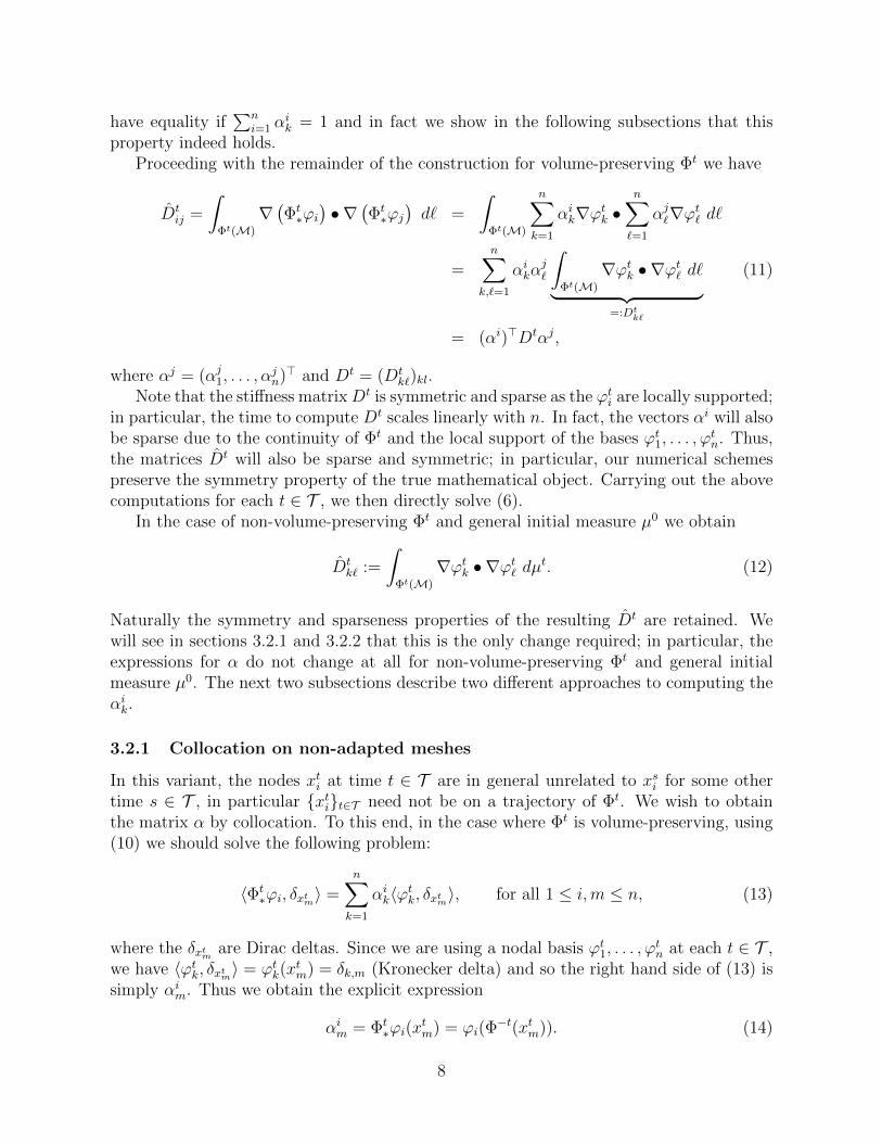
Cauchy-Green approach. We use T = 0, 1 and employ Gauss quadrature of degree 5(7 quadrature nodes, using fewer points yields degraded results) for the numerical integra-tion of (9). Figure 1 shows the spectra and Figures 2 and 3 the 2nd and 3rd eigenvectorsas well as the resulting decomposition into coherent sets on a triangulation of 25 × 25equidistant points (1152 triangles) as well as on the Delaunay triangulation of a set of625 scattered nodes (1236 triangles), respectively. Already at this comparatively low res-olution, the results are broadly similar to those in [19]. Note, however, that we need toevaluate C−1

t (for which we evaluate DΦt by finite differencing) at roughly 8000 points,

14

which takes around 2 seconds. The assembly of the matrices takes 0.02 s and the solutionof the eigenproblem 0.05 seconds4.

Figure 1: Rotating double gyre: spectrum of the dynamic Laplacian on a triangulation ofa regular 25 × 25 grid (left) and of 625 scattered points (right) using the approach fromSection 3.1.

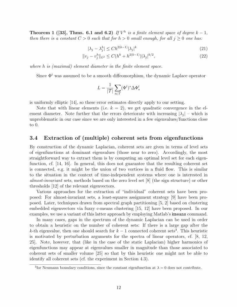
Figure 2: Rotating double gyre: 2nd and 3rd eigenvector as well as the resulting coherentpartition (from left to right) on a triangulation of a regular 25× 25 grid using the Cauchy-Green approach from Section 3.1. The tensor C−1

t is evaluated at 8064 points.

Transfer operator approach. We repeat the same experiment with T = 0, 1 usingthe approach from Section 3.2.1. Figure 4 (left) shows the spectrum, Figure 5 the 2nd and3rd eigenvectors as well as the resulting coherent 3-partition. Here, the inverse flow map(without variational equation) had to be evaluated 25 · 25 = 625 times only, which takes0.1 s, the assembly of the matrices takes 0.02 s and the solution of the eigenproblem again0.1 seconds. Note that the only data that we input to our method is the initial and finalpositions of the 625 nodes.

4All timings measured on a dual core Intel i5 with 2.4 GHz and Matlab R2016a.

15

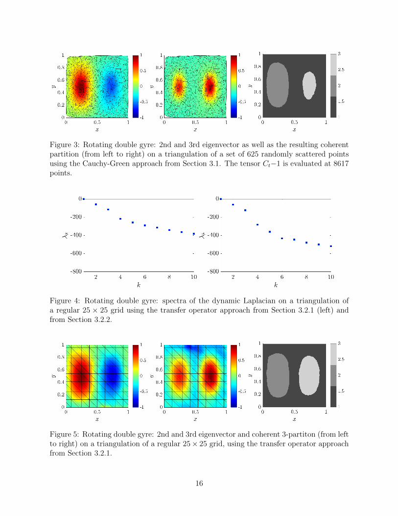
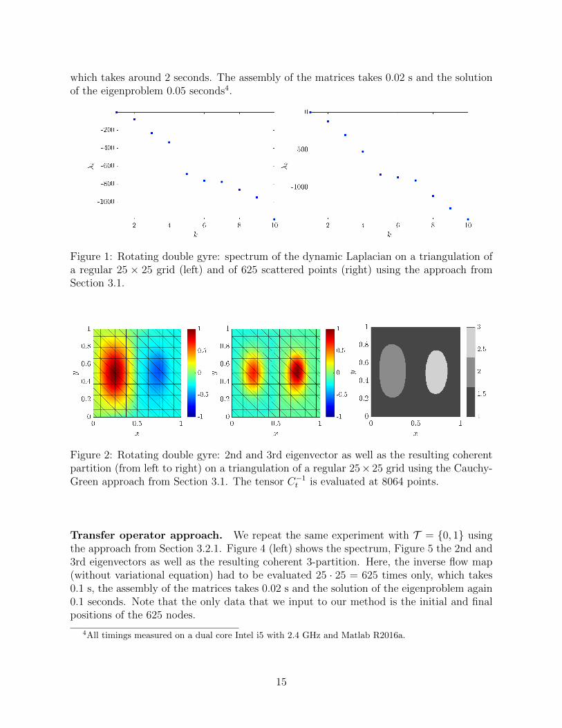
Figure 3: Rotating double gyre: 2nd and 3rd eigenvector as well as the resulting coherentpartition (from left to right) on a triangulation of a set of 625 randomly scattered pointsusing the Cauchy-Green approach from Section 3.1. The tensor Ct−1 is evaluated at 8617points.

Figure 4: Rotating double gyre: spectra of the dynamic Laplacian on a triangulation ofa regular 25 × 25 grid using the transfer operator approach from Section 3.2.1 (left) andfrom Section 3.2.2.

Figure 5: Rotating double gyre: 2nd and 3rd eigenvector and coherent 3-partiton (from leftto right) on a triangulation of a regular 25× 25 grid, using the transfer operator approachfrom Section 3.2.1.

16

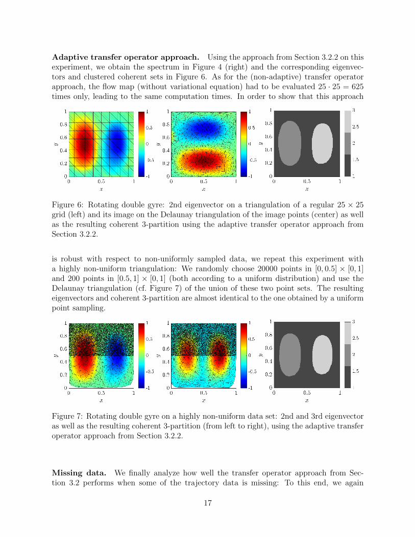
Adaptive transfer operator approach. Using the approach from Section 3.2.2 on thisexperiment, we obtain the spectrum in Figure 4 (right) and the corresponding eigenvec-tors and clustered coherent sets in Figure 6. As for the (non-adaptive) transfer operatorapproach, the flow map (without variational equation) had to be evaluated 25 · 25 = 625times only, leading to the same computation times. In order to show that this approach

Figure 6: Rotating double gyre: 2nd eigenvector on a triangulation of a regular 25 × 25grid (left) and its image on the Delaunay triangulation of the image points (center) as wellas the resulting coherent 3-partition using the adaptive transfer operator approach fromSection 3.2.2.

is robust with respect to non-uniformly sampled data, we repeat this experiment witha highly non-uniform triangulation: We randomly choose 20000 points in [0, 0.5] × [0, 1]and 200 points in [0.5, 1] × [0, 1] (both according to a uniform distribution) and use theDelaunay triangulation (cf. Figure 7) of the union of these two point sets. The resultingeigenvectors and coherent 3-partition are almost identical to the one obtained by a uniformpoint sampling.

Figure 7: Rotating double gyre on a highly non-uniform data set: 2nd and 3rd eigenvectoras well as the resulting coherent 3-partition (from left to right), using the adaptive transferoperator approach from Section 3.2.2.

Missing data. We finally analyze how well the transfer operator approach from Sec-tion 3.2 performs when some of the trajectory data is missing: To this end, we again

17

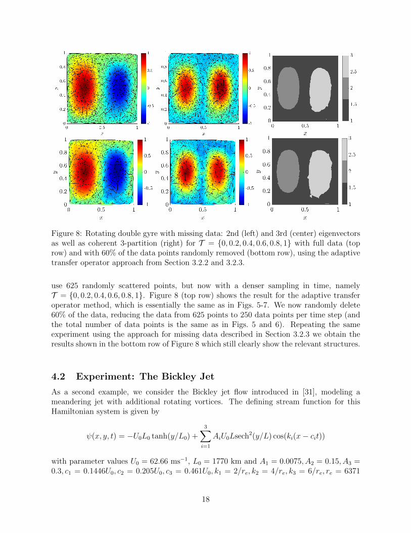
Figure 8: Rotating double gyre with missing data: 2nd (left) and 3rd (center) eigenvectorsas well as coherent 3-partition (right) for T = 0, 0.2, 0.4, 0.6, 0.8, 1 with full data (toprow) and with 60% of the data points randomly removed (bottom row), using the adaptivetransfer operator approach from Section 3.2.2 and 3.2.3.

use 625 randomly scattered points, but now with a denser sampling in time, namelyT = 0, 0.2, 0.4, 0.6, 0.8, 1. Figure 8 (top row) shows the result for the adaptive transferoperator method, which is essentially the same as in Figs. 5-7. We now randomly delete60% of the data, reducing the data from 625 points to 250 data points per time step (andthe total number of data points is the same as in Figs. 5 and 6). Repeating the sameexperiment using the approach for missing data described in Section 3.2.3 we obtain theresults shown in the bottom row of Figure 8 which still clearly show the relevant structures.

4.2 Experiment: The Bickley Jet

As a second example, we consider the Bickley jet flow introduced in [31], modeling ameandering jet with additional rotating vortices. The defining stream function for thisHamiltonian system is given by

ψ(x, y, t) = −U0L0 tanh(y/L0) +3∑i=1

AiU0Lsech2(y/L) cos(ki(x− cit))

with parameter values U0 = 62.66 ms−1, L0 = 1770 km and A1 = 0.0075, A2 = 0.15, A3 =0.3, c1 = 0.1446U0, c2 = 0.205U0, c3 = 0.461U0, k1 = 2/re, k2 = 4/re, k3 = 6/re, re = 6371

18

km as in [22]. We consider the associated flow on the domain M = [0, 20] × [−3, 3] withperiodic boundary conditions in x-direction on the time interval t ∈ [0, 40] days.

Cauchy-Green approach. Employing T = 0, 40 and the Delaunay triangulation ona regular grid of 100 × 30 points as well as Gauss quadrature of degree 1, we obtain theresults shown in Figure 10. The evaluation of C−1

t on roughly 6000 quadrature nodes takesabout 8 s, the assembly of the matrices 0.07 s and the solution of the eigenproblem 0.4seconds.

Figure 9: Bickley jet: Spectrum (left), 2nd (right top) and 3rd (right center) eigenvectorand a coherent 7-partition (right bottom) on a triangulation of a regular 100× 30 grid ofnodes using the Cauchy-Green approach from Section 3.1.

Adaptive transfer operator approach. Using the same triangulation as for the Cauchy-Green approach, we obtain the results shown in Figure 10. The evaluation of the flow mapon the 3000 nodes of the triangulation takes 1 s, the assembly of the matrices 0.1 s andthe solution of the eigenproblem 0.5 seconds.

Missing data. In order to analyze the performance when some of the data is missingwe use the same 100 × 30 grid, but now with ten intermediate time samplings of thetrajectories, i.e. T = 0, 4, 8, . . . , 40. The result of the adaptive transfer operator approachis essentially the same as in Fig. 10. We then randomly delete 80% of the data, reducingit from 3000 points to 600 points per time step, which in total yields the same number ofdata points as with T = 0, 40 and no missing data. The approach from Section 3.2.3leads to the results shown in Fig. 11, still clearly showing the relevant structures.

19

Figure 10: Bickley jet: Spectrum (left), 2nd (right top) and 3rd (right center) eigenvectorand a coherent 8-partition (right bottom) on a triangulation of a regular 100× 30 grid ofnodes using the adaptive transfer operator approach from Section 3.2.2.

Figure 11: Bickley jet with missing data: Spectrum (left), 2nd (right top) and 3rd (rightcenter) eigenvector as well as coherent 8-partition (right bottom) with 80% of the datarandomly removed (cf. Fig. 10).

20

4.3 Experiment: Ocean flow from satellite data

We now consider an unsteady velocity field derived from AVISO satellite altimetry mea-surements in the domain of the Agulhas leakage in the South Atlantic Ocean. Under theassumption of geostrophicity, the sea surface height h yields a stream function for thevelocity of water at the surface and the corresponding equations of motion for particletrajectories are

ϕ = −A(θ)∂θh(ϕ, θ, t) (23)

θ = A(θ)∂ϕh(ϕ, θ, t), (24)

where ϕ is the longitude and θ the latitude of a particle, A(θ) = g/R22Ω sin θ cos θ, gis the gravitational constant, R is the mean radius of the earth and Ω the earth’s meanangular velocity. We choose the same spatial and termporal domain as in [21], namely[−4, 6]× [−34,−28] and a period of 90 days, from t0 = Nov 11, 2006 on. Figure 12 showsthe forward finite time Lyapunov exponent field of the data.

Figure 12: Ocean flow: FTLE field (log10 color coding)

After a flow duration of 90 days the initial rectangular domain shown in Figure 12 be-comes strongly distorted and filamented. In this situation, we are not interested in coherentsets that intersect this heavily filamented boundary and so we restrict to coherent sets inthe interior of the domain. This can be achieved by replacing the (natural) homogeneousNeumann boundary conditions with homogeneous Dirichlet boundary conditions. In termsof numerical eigenvector computations, to apply homogeneous Dirichlet boundary condi-tions, one simply sets all rows and columns of Dt and M in (7) corresponding to nodes onthe boundary of the domain to rows and columns of zeros.

Cauchy-Green approach. As in [21], we use a uniform grid of 250 × 150 points, theassociated Delaunay triangulation, yielding roughly 73000 triangles and Gauss quadratureof degree 1 (i.e. one quadrature point per element). The evaluation of C−1

t takes ca. 46 s,the assembly of the matrices 0.3 s and the solution of the eigenproblem 3 seconds.

21

Figure 13 (left) shows the largest 10 eigenvalues of the dynamic Laplacian with T =t0, t0 + 90 (the results do not change significantly when using more intermediate timesteps), Figure 14 (left column) the first three eigenvectors. Note that there appears to be agap after the third eigenvalue. The corresponding coherent sets (as identified by k-meansclustering the first three eigenvectors, cf. Fig. 15 (left)) nicely agree with those identified in[21], Fig. 9. The rightmost vortex from Fig. 9 in that work, however, is missing from thiscomputation. It is, however, identified by the 9th eigenfunction (cf. Figs. 16 (left) and 17(left)). Note that due to the variational characterization of the eigenvalues, the magnitudeof the eigenvalue indicates how much this set resists filamentation (cf. Fig. 18).

We deliberately chose the same resolution as in [21] here, the results for the leadingthree eigenvectors do not change significantly when decreasing the grid resolution down to100× 60 points only.

Figure 13: Ocean flow: spectrum of the dynamic Laplacian using the Cauchy-Green ap-proach (left) and the adaptive transfer operator approach (right).

Adaptive transfer operator approach. The approach from Section 3.2.2 yields com-parable results as shown in the right columns of Figs. 13–17. The computation times are:time integration: 4 s, assembly: 1.4 s, solution of the eigenproblem: 16 seconds.

Here, we can decrease the resolution down to a 150× 90 grid before the results start todeteriorate significantly.

Missing data. We finally analyze how well the coherent sets can be recovered in theocean flow experiment when data is missing. Again, we use the same set of nodes and|T | = 10 equidistant intermediate time steps. We then randomly delete 70% of the data,yielding roughly 12000 data points per time step. For comparison, in the experiment withfull data and two time steps above we used around 37500 nodes per time step. The resultshown in Figure 19 are qualitatively the same as the one with full data in Figure 14.We note, however, that when we delete even more data, these coherent sets will not berecovered as clearly any more.

22

Figure 14: Ocean flow: the first three eigenvectors of the dynamic Laplacian using theCauchy-Green approach (left) and the adaptive transfer operator approach (right).

Figure 15: Ocean flow: coherent sets identified using the first 3 eigenfunctions by theCauchy-Green approach (left) and by the adaptive transfer operator approach (right).

23

Figure 16: Ocean flow: 9th eigenfunction from the Cauchy-Green approach (left) and 6theigenfunction from the adaptive transfer operator approach (right).

Figure 17: Ocean flow: coherent sets identified using the 1st, 2nd, 3rd and 9th eigenfunctionby the Cauchy-Green approach (left) and using the 1st, 2nd, 3rd and 6th eigenfunction bythe adaptive transfer operator approach (right).

Figure 18: Ocean flow: coherent sets from Fig. 17 (left) and their images (gray) as well asa non-coherent set and its image (blue).

24

Figure 19: Ocean flow with missing data: coherent sets based on the adaptive transferoperator approach from Section 3.2.2 with 10 intermediate time steps and 70% of the datarandomly removed.

4.4 Experiment: The unsteady ABC flow (3D)

For a 3D experiment, we consider the unsteady ABC flow, cf. [23], given by

x = (A+ 12t sin(πt)) sin z + C cos y (25)

y = B sinx+ (A+ 12t sin(πt)) cos z (26)

z = C sin y +B cosx (27)

with parameter values A =√

3, B =√

2, C = 1 on the time interval t ∈ [0, 1].

Cauchy-Green approach. We employ the Delaunay triangulation on a regular gridof 25 × 25 × 25 = 15625 points, yielding about 83000 tetrahedra, Gauss quadrature ofdegree 1, i.e. one quadrature point per tetrahedron and two time steps, i.e. T = 0, 1.The integration of the variational equation takes 14 seconds, the assembly of the matrices 7seconds and the solution of the eigenproblem 5 seconds. Figure 20 (left) shows the spectrumof the discrete dynamic Laplacian, Figure 21 (right) the 2nd and 3rd eigenvector.

Non-adaptive transfer operator approach. Using the same parameters as for theCauchy-Green approach, we obtain the spectrum shown in Figure 20 (right) and the eigen-vectors in Figure 21 (right). While this yields qualitatively the same results as the Cauchy-Green approach, the eigenfunctions are less smooth in this case because the flow is realanalytic and in contrast to the CG approach, this method does not use derivative informa-tion. Computation times are: assembly 6, computation of the α-matrix 3 and eigenproblem100 seconds – which is due to the fact that the stiffness matrix has 2.5 million nonzeroentries which is 100 times as much as for the CG approach (cf. the remark in Section 3.2.1on the sparseness of the stiffness matrix in this case).

We expect the adaptive transfer operator approach to be much faster as α need not beconstructed. We did not apply the adaptive transfer operator approach for this examplefor coding convenience, since it would require a periodization of a scattered set of nodes.

25

Figure 20: ABC flow: Spectrum of the dynamic Laplacian for the Cauchy-Green (left) andthe transfer operator approach (right).

Figure 21: ABC flow: 2nd (top) and 3rd (bottom) eigenvector using the Cauchy-Green(left column) and the transfer operator approach (right column) from Section 3.2.1.

26

Acknowledgements

We thank Daniel Karrasch for helpful comments and contributions to the code, and MichaelFeischl for helpful comments. GF thanks the Department of Mathematics at the TechnicalUniversity Munich for hospitality during a visit in May 2016, and the John von NeumannProfessorship scheme for financial support for this visit. GF was supported by an ARCFuture Fellowship. OJ was supported by the Priority Programme SPP 1881 TurbulentSuperstructures of the Deutsche Forschungsgemeinschaft.

A The non volume-preserving case

We now briefly sketch the theory behind the case of the underlying flow Φt not beingvolume-preserving, where we wish to track coherent masses according to some smoothinitial mass distribution on M ⊂ Rd given by a probability measure µ0 (µ0 = m wouldcorrespond to volume), and where the domain is possibly curved with the curvature de-scribed by a Riemannian metric. The measure µ0 is evolved by Φt according to µt := µΦ−t.All computational aspects for data embedded in Eulidean space are described in Section3.

The expressions (1) and (3) can be naturally extended to cover this situation. Firstly(1), where the size of the disconnector Γ is computed according to the evolved measure µt:

h(Γ) :=

1|T |∑

t∈T µd−1,t(ΦtΓ)

minµd−1,0(M1), µd−1,0(M2),

where µd−1,t is the induced measure on d− 1-dimensional surfaces at time t. Secondly, (3),

s := inff∈C∞(M,R)

1|T |∑

t∈T ‖(|∇mtΦt∗f |mt)‖µt

infα ‖f − α‖µ0,

where the subscripts mt denote that the computations are taken with respect to the Rie-mannian metric mt on Φt(M), which in many cases will be either the Euclidean metric, orif M is of dimension lower than d, the induced metric arising from the Euclidean metric.See [17] for details.

Finally, we replace (4) with(1

|T |∑t∈T

(Φt)∗∆µtΦt∗

)v = λv (28)

where ∆µt is the µt-weighted Laplace operator on Φt(M) (see [17] for details).The weak form of the eigenproblem (28) can be written as [17]

1

|T |∑t∈T

∫Φt(M)

∇(Φt∗ψ) · ∇(Φt

∗v) dµt = λ

∫Mψv dµ, for all ψ ∈ C∞(Ω).

Again, if we want to have a continuous-time version of the above eigenproblem, we simplyreplace the average over t ∈ T with an integral.

27

B Appendix: Code example

We here provide sample code which performs the computations reported on in Section 4.1.Note that this code has been stripped down for readability. A more efficient version canbe downloaded from https://github.com/gaioguy/FEMDL.

1 clear all

2 % flow map , data points and time integration

3 t0 = 0; tf = 1; nt = 5;

% init , final time , steps

4 T = @(x) flow_map(x,linspace(t0,tf,nt));

5 n = 625; p0 = rand(n,2); % data points

6 P = T(p0); for k = 1:nt, pk=P(:,[k k+nt]); end; % time integration

7

8 % assembly

9 D = sparse(n,n);

10 for k = 1:nt

11 tk = delaunay(pk);

12 [Dt ,M] = assemble(pk,tk);

13 D = D + Dt/nt;

14 end;

15

16 % solve eigenproblem

17 [V,L] = eigs(D,M,10,’SM’);

18 [lam ,I] = sort(diag(L),’descend ’); V = V(:,I);

19

20 % compute coherent partition

21 m = 200; x = linspace (0,1,m); [X,Y] = ndgrid(x,x);

22 k = 3; for j = 1:k,

23 v = scatteredInterpolant(p0(:,1),p0(:,2),V(:,j));

24 W(:,j) = reshape(v(X,Y),m*m,1);

25 end

26 idx = kmeans(W,k);

27

28 % plot spectrum , 2nd eigenvector and partition

29 figure (1); clf; plot(lam ,’*’); title(’spectrum ’)

30 figure (2); clf; trisurf(t1,p0(:,1),p0(:,2), zeros(n,1),V(: ,2));

31 shading interp , view(2), axis equal , axis tight , colorbar

32 hold on , triplot(t1,p0(:,1),p0(:,2),’k’); title(’2nd eigenvector ’);

33 figure (3); clf; surf(X,Y,reshape(idx ,m,m)); shading flat

34 view(2), axis equal , axis tight , title(’coherent partition ’)

Code 1: main script for the rotating double gyre flow, using the adaptive transfer operatormethod

28

1 function [D,M] = assemble(p,t)

2

3 % p: n by 2 matrix of nodes , t: m by 3 matrix , defining the triangles

4 % based on http :// math.mit.edu/~gs/cse/codes/femcode.m by G. Strang

5 % Note: for large n, this code is inefficient , use FEMDL instead

6

7 n = size(p,1); % number of nodes

8 D = sparse(n,n); M = sparse(n,n);

9 for e = 1:size(t,1) % integration over each element

10 ns = t(e,:); % nodes of triangle e

11 P = [ones(3,1),p(ns ,:)]; % 3 x 3 matrix with rows = [1 x y]

12 area = abs(det(P))/2; % area of triangle e

13 B = inv(P);

14 grad = B(2:3 ,:); % gradients of shape funtions

15 D(ns ,ns) = D(ns,ns) - area*grad ’*grad;

16 M(ns ,ns) = M(ns,ns) + area /12*( ones (3 ,3)+eye (3));

17 end

Code 2: assembly of stiffness and mass matrix.

1 function y = flow_map(x,tspan)

2

3 function dz = v(t,z) % vector field of the rotating double gyre

4 n = numel(z)/2;

5 x = z(1:n,1); y = z(n+1:2*n,1);

6 st = ((t >0)&(t <1)).*t.^2.*(3 -2*t) + (t >1)*1;

7 dxPsi_P = 2*pi*cos (2*pi*x).* sin(pi*y);

8 dyPsi_P = pi*sin (2*pi*x).* cos(pi*y);

9 dxPsi_F = pi*cos(pi*x).* sin (2*pi*y);

10 dyPsi_F = 2*pi*sin(pi*x).* cos (2*pi*y);

11 dz(n+1:2*n,1) = (1-st).* dxPsi_P + st.* dxPsi_F;

12 dz(1:n,1) = -((1-st).* dyPsi_P + st.* dyPsi_F );

13 end

14

15 [~,F] = ode45(@v,tspan ,[x(:,1); x(: ,2)]);

16 y = [F(:,1:end/2)’ F(:,end /2+1: end)’];

17 end

Code 3: the flow map for the rotating double gyre flow.

References

[1] F. Alouges. A new finite element scheme for Landau-Lifchitz equations. DiscreteContin. Dyn. Syst. Ser. S, 1(2):187–196, 2008.

[2] C. J. Alpert, A. B. Kahng, and S.-Z. Yao. Spectral partitioning with multiple eigen-vectors. Discrete Applied Mathematics, 90(1-3):3–26, 1999.

[3] V. Blasjo. The isoperimetric problem. Amer. Math. Monthly, 112(6):526–566, 2005.

29

[4] M. Budisic and I. Mezic. Geometry of the ergodic quotient reveals coherent structuresin flows. Physica D: Nonlinear Phenomena, 241(15):1255–1269, 2012.

[5] P. K. Chan, M. D. Schlag, and J. Y. Zien. Spectral k-way ratio-cut partitioning andclustering. IEEE Transactions on Computer-Aided Design of Integrated Circuits andSystems, 13(9):1088–1096, 1994.

[6] L. Chen. iFEM: an integrated finite element methods package in MATLAB, 2008.

[7] F. R. Chung. Spectral graph theory, volume 92. American Mathematical Soc., 1997.

[8] M. Dellnitz and O. Junge. On the approximation of complicated dynamical behavior.SIAM Journal on Numerical Analysis, 36(2):491–515, 1999.

[9] P. Deuflhard, W. Huisinga, A. Fischer, and C. Schutte. Identification of almost in-variant aggregates in reversible nearly uncoupled Markov chains. Linear Algebra andits Applications, 315(1-3):39–59, 2000.

[10] H. Edelsbrunner, D. Kirkpatrick, and R. Seidel. On the shape of a set of points in theplane. IEEE Transactions on Information Theory, 29(4):551–559, Jul 1983.

[11] G. E. Fasshauer. Meshfree approximation methods with MATLAB, volume 6 of Inter-disciplinary Mathematical Sciences. World Scientific Publishing Co. Pte. Ltd., Hack-ensack, NJ, 2007. With 1 CD-ROM (Windows, Macintosh and UNIX).

[12] G. Froyland. Statistically optimal almost-invariant sets. Physica D, 200(3):205–219,2005.

[13] G. Froyland. An analytic framework for identifying finite-time coherent sets in time-dependent dynamical systems. Physica D, 250:1–19, 2013.

[14] G. Froyland. Dynamic isoperimetry and the geometry of Lagrangian coherent struc-tures. Nonlinearity, 28(10):3587, 2015.

[15] G. Froyland and M. Dellnitz. Detecting and Locating Near-Optimal Almost-InvariantSets and Cycles. SIAM Journal on Scientific Computing, 24(6):1839–1863, Jan. 2003.

[16] G. Froyland and O. Junge. On fast computation of finite-time coherent sets usingradial basis functions. Chaos, 25(8):087409, 2015.

[17] G. Froyland and E. Kwok. A dynamic Laplacian for identifying Lagrangian co-herent structures on weighted Riemannian manifolds. Submitted. Available athttps://arxiv.org/abs/1610.01128.

[18] G. Froyland, S. Lloyd, and N. Santitissadeekorn. Coherent sets for nonautonomousdynamical systems. Physica D, 239(16):1527–1541, 2010.

[19] G. Froyland and K. Padberg-Gehle. A rough-and-ready cluster-based approach forextracting finite-time coherent sets from sparse and incomplete trajectory data. Chaos,25(8):087406, 2015.

30

[20] G. Froyland, N. Santitissadeekorn, and A. Monahan. Transport in time-dependentdynamical systems: Finite-time coherent sets. Chaos, 20(4):043116, 2010.

[21] A. Hadjighasem and G. Haller. Level set formulation of two-dimensional Lagrangianvortex detection methods. Chaos, 26(10):103102, 2016.

[22] A. Hadjighasem, D. Karrasch, H. Teramoto, and G. Haller. Spectral-clustering ap-proach to Lagrangian vortex detection. Physical Review E, 93(6):063107, 2016.

[23] G. Haller. Distinguished material surfaces and coherent structures in three-dimensional fluid flows. Physica D, 149:248–277, 2001.

[24] G. Haller and F. J. Beron-Vera. Coherent Lagrangian vortices: The black holes ofturbulence. Journal of Fluid Mechanics, 731:R4, 2013.

[25] D. Karrasch and J. Keller. A geometric heat-flow theory of Lagrangian coherentstructures. Submitted. Available at https://arxiv.org/abs/1608.05598.

[26] R. MacKay, J. Meiss, and I. Percival. Transport in Hamiltonian systems. Physica D:Nonlinear Phenomena, 13(1-2):55–81, 1984.

[27] G. Mathew, I. Mezic, and L. Petzold. A multiscale measure for mixing. Physica D:Nonlinear Phenomena, 211(1):23–46, 2005.

[28] I. Mezic and S. Wiggins. A method for visualization of invariant sets of dynamicalsystems based on the ergodic partition. Chaos, 9(1):213–218, 1999.

[29] B. A. Mosovsky and J. D. Meiss. Transport in transitory dynamical systems. SIAMJournal on Applied Dynamical Systems, 10(1):35–65, 2011.

[30] V. Rom-Kedar and S. Wiggins. Transport in two-dimensional maps. Archive forRational Mechanics and Analysis, 109(3):239–298, 1990.

[31] I. I. Rypina, M. G. Brown, F. J. Beron-Vera, H. Kocak, M. J. Olascoaga, and I. A.Udovydchenko. On the Lagrangian dynamics of atmospheric zonal jets and the per-meability of the stratospheric polar vortex. Journal of the Atmospheric Sciences,64(10):3595–3610, 2007.

[32] G. Strang. Computational science and engineering. Wellesley-Cambridge Press,Wellesley, MA, 2007. http://math.mit.edu/~gs/cse/.

[33] G. Strang and G. J. Fix. An analysis of the finite element method. Prentice-Hall, Inc.,Englewood Cliffs, N. J., 1973. Prentice-Hall Series in Automatic Computation.

[34] J.-L. Thiffeault. Using multiscale norms to quantify mixing and transport. Nonlin-earity, 25(2):R1, 2012.

[35] S. M. Ulam. A collection of mathematical problems, volume 8. Interscience Publishers,1960.

31

[36] R. Vanselow. About Delaunay triangulations and discrete maximum principles for thelinear conforming FEM applied to the Poisson equation. Applications of Mathematics,46(1):13–28, 2001.

[37] H. Wendland. Scattered data approximation, volume 17 of Cambridge Monographs onApplied and Computational Mathematics. Cambridge University Press, Cambridge,2005.

32