Robust Face Recognition Technique with ANFIS in Compared ...ijcim.th.org/past_editions/2018V26N1/26n1Page82.pdf · order to calculate Histogram cell relationship Fig. 2 whereby Pixel

International Journal of the Computer, the Internet and Management Vol.26 No.1 (January-April, 2018) pp. 82-95

82

Robust Face Recognition Technique

with ANFIS in Compared with Feedforward

Backpropagation Neural Network

Using Specific Features of Wavelet

Transform and HOG

Thoedsak Sukdao1,

Surasak Mungsing2,

Department of Information Technology,

Sripatum University, Thailand [email protected]

[email protected]

and Katanyoo Klabsuwan3

CEO E-ideas Co., ltd., Thailand [email protected]

Abstract - The aims of the research were to

study a face recognition using ANFIS

(Adaptive Neuro-Fuzzy Inference System)

technique to compared with feedforward

backpropagation neural network that used

specific Features of Wavelet Transform and

HOG (Histogram of Oriented Gradients for

feature extraction). The result found that

the accuracy of ANFIS face recognition

technique was 99% and feedforward back

propagation neural network was 98 %.

Keywords - Face Recognition, ANFIS (Adaptive

Neuro-Fuzzy Inference System), Feedforward

Backpropagation Neural Network, Wavelet

Transform, HOG (Histogram of Oriented

Gradients for Feature Extraction)

I. INTRODUCTION

A. Statement of the Problems

The use of Face Recognition to prove an

identity by using Digital Image Processing [1]

as various theories are used for example; a

detection using Harr Feature method and bring

Harr Feature method to apply with a color

model RGB-HSVYcbCr [2] the color model

used will help solve problems in the area of

unequal dispersed color by using Histogram

Equalization [3] to help correct the picture

features for improvement and by using the

primary color model the face recognition can

bear with lighting conditions which makes the

face recognition more accurately or using Face

Detection features[4] i.e. eyes nose mouth as

primary features to use in finding positions for

detection reference by Template Matching

theory [5] to find the closest picture with

Template Matching or using Face Recognition

[6] by using various theories i.e. detecting

main factors of face features [7] to detect

pictures to indicate that the detected Face

Recognition picture is matching with others or

using other arithmetic means to consider an

increase in efficiency for several personal

recognition [6] by using I-Gain method or the

Neural network back propagation together with

the Color Model [6] in order to use a Face

Recognition more efficiently.

Face Recognition is important and considering a

branch of an Artificial Intelligence. There are

many types of Recognition i.e. a letter

recognition, a sound recognition, a face

recognition etc. A face recognition has an

important process in which a picture from a

Thoedsak Sukdao, Surasak Mungsing, and Katanyoo Klabsuwan


83

camera is transformed from RGB to gray color

and adjust size to 80x100 Pixel to become

medium size then import by extracting

features of Wavelet transform using Single-

level discrete 2-D wavelet transform. The

result will be Vector 72 member size then

import HOG (Histogram of oriented gradients).

HOG is set up to 15x15 Pixel then import

algorithm for both techniques of recognition,

ANFIS and Neural network back propagation,

to compare the test result efficiency of face

recognition further.

The Haar-Like Feature Detection technique

is developed from the method of Viola and

Jones which is a method to detect an object in

the picture by building features indicating the

differences between white and black color.

This method helps enable feature detections

required even in a little light condition. This

research brings a pattern of the feature

detections to apply in the process of face

recognition detection and proposes an

uncomplicated method by extracting specific

feature techniques of Single-level discrete 2-D

wavelet transform then input image. Thereafter,

inputting HOG before entering ANFIS

technique and Neural Network which makes

the system efficient and enable to detect face

recognition accurately. Topic #2 will explain

about the method used, Topic#3 the details of

system development, Topic# 4 the testing

method and discussion, Topic#5 a conclusion

of the research.

B. Objectives

To develop a method and to increase an

efficiency in face recognition system by using

whole face features together with a specific

face features comparison using ANFIS (Adaptive

Neuro-Fuzzy Inference System) technique to

compare with neural network back propagation then

apply specific feature of Wavelet transform

and HOG.

C. Scope of Study

The development of increasing an efficiency of

face recognition system using face features

coupled with specific face features of the

following scopes as follows;

A motion picture experimented a video pictures from a computer.

A motion picture experimented an

uncomplicated background picture.

A motion picture experimented a straight face with emotions i.e. smile, laugh, speak,

etc.

A motion picture experimented with unequal lighting environment.

A motion picture experimented a single man or woman.

II. THEORY

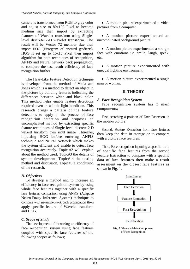
A. Face Recognition System

Face recognition system has 3 main

components:

First, searching a position of Face Detection in

the motion picture.

Second, Feature Extraction from face features

then keep the data in storage or to compare

with a picture face features.

Third, Face recognition inputting a specific data

of specific face features from the second

Feature Extraction to compare with a specific

data of face features then make a result

assessment on the closest face features as

shown in Fig. 1.

Fig. 1 Shows a Main Component

of Face Recognition

Robust Face Recognition Technique with ANFIS in Compared with Feedforward Backpropagation Neural Network

Using Specific Features of Wavelet Transform and HOG


84

B. Wavelet – Based Transformation

Wavelet – Based Transformation has an

influence from Fourier Analysis method using

an analysis of discontinued wavelet whereby

Fourier capability can only be found in the

existing frequency in order to further develop

a short time Fourier to learn that the frequency

will by exist in which period of time by using

Window functions to compare a Wavelet.

However, a Short time Fourier capability is

still limited in terms of the unknown existing

frequency at any point. This development

becomes a Wavelet – Based Transformation in

which the analysis is focused on scale and a

study of Resolution.

Wavelet is a function that is not a new

concept but an existing function has been used

since 1800 by Joseph Fourier who found this

function by laying down sines and cosines to

replace other functions. However, in order to

analyze scales, the Algorithm Wavelet can be

used to manage the data that has different

scale or resolution. If looking at a large

window, a clear outstanding feature can be

noticed. On the other hand, if looking at a

small window a small outstanding feature can

be also noticed.

C. HOG (Histogram of Oriented Gradients

for Feature Extraction)

Capturing a superiority of face by explaining a

picture from the frequency value of direction

from gradients is the method to capture

features in the picture by dispersing the

gradient’s deepness or the direction’s border

by separating pictures in small cells. Within a

cell, it is composed of Gradients’ direction

kept in Histogram format in which the cell

characteristics can be explained to increase an

effectiveness in accuracy and to be able to

normalize by calculating an indicator of

deepness from the cell overlapped in the

picture in blocks to reduce the impact from a

light change and less shade. The Gradients

assessment can be found from using ID -

discrete derivative masks. Finding the first

derivatives from vertical and horizontal axis

by the method of [-1, 0, 1] and [-1, 0, 1]T to

formulate values of mask in x and y axis in

order to calculate Histogram cell relationship

whereby Pixel in the cell will have direction

and weight from Gradients’ calculation and

finding a picture’s direction resulting in a

picture explanation in Histogram format.

D. Adaptive Neuro-Fuzzy Inference System:

ANFIS

ANFIS is a Fuzzy model which is

mentioned and brought to apply in various

work within ANFIS applied and integrated in

both Neural network back propagation and

Fuzzy. This makes strong advantages of each

model to support and to reduce each model

limitation for a model learning data adjustment

as it is a strength of Neural network back

propagation. However, the limitation in explaining a

model learning integration is quite difficult to

communicate to understand comparing with

general human perspectives or general

communication. The basis of Fuzzy model

developed from Crisp Logic by comparing the

rule If-Then to decide ambiguously or Fuzzy

Logic.

The Basic Fuzzy models, Mandani Fuzzy

and Sugeno, are mentioned. Both methods

have some differences in Output function

value and Output Membership Function. The

latter method can choose either the Line

function or Constant function. In this case,

ANFIS model is developed from Sugeno

Fuzzy.

1. Sugeno Fuzzy structure or TS: Takagi-

Sugeno Fuzzy is shown in Fig. 2. The data

sample input in 2 dimensions is brought to be

assessed in function and Input Membership

Function. The result to be used to determine

Rule Weight or Firing Strength for the variable

assessment from an output and a relationship

of an equation (1) can be exhibited.

Fig. 2 Fuzzy Structure Model Sugeno Fuzzy



85

(1)

n represents a number of Fuzzy rule.

Whereby, w is resulted from comparing values

of Fuzzy rules received from the Input

Membership Function as determined by

specialists to choose various functions in many

models. In this research, Gaussian Function is

selected due to the dispersed data which is in

line with a Function. Gaussian Function in

output membership (Output MF) can be

chosen from 2 models; Zero Order or

determining the output membership by a

constant number to set a=b=0 and the First

Order or set by a Line equation z = ax1 + bx2 +

c. In case of ANFIS application, the latter

model is chosen by showing a relationship

between Sugeno Fuzzy model and ANFIS in

the next topic.

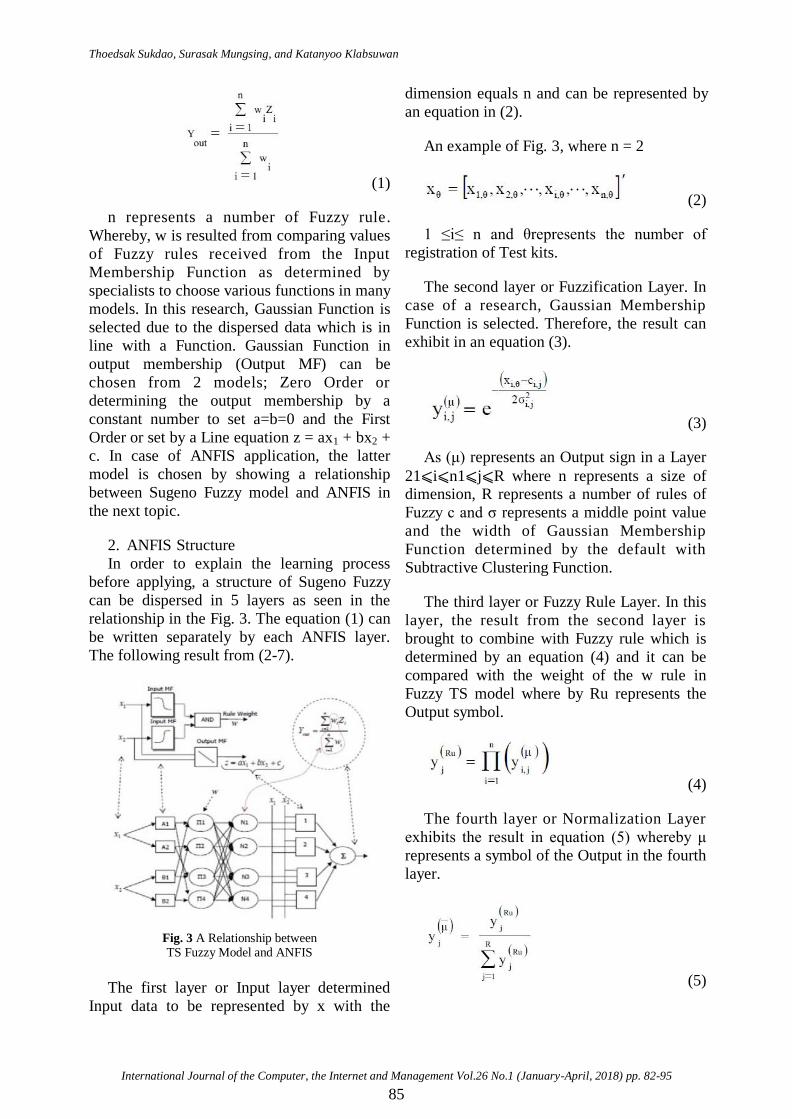
2. ANFIS Structure

In order to explain the learning process

before applying, a structure of Sugeno Fuzzy

can be dispersed in 5 layers as seen in the

relationship in the Fig. 3. The equation (1) can

be written separately by each ANFIS layer.

The following result from (2-7).

Fig. 3 A Relationship between TS Fuzzy Model and ANFIS

The first layer or Input layer determined

Input data to be represented by x with the

dimension equals n and can be represented by

an equation in (2).

An example of Fig. 3, where n = 2

(2)

1 ≤i≤ n and θrepresents the number of

registration of Test kits.

The second layer or Fuzzification Layer. In

case of a research, Gaussian Membership

Function is selected. Therefore, the result can

exhibit in an equation (3).

(3)

As (μ) represents an Output sign in a Layer

21⩽i⩽n1⩽j⩽R where n represents a size of dimension, R represents a number of rules of

Fuzzy c and σ represents a middle point value

and the width of Gaussian Membership

Function determined by the default with

Subtractive Clustering Function.

The third layer or Fuzzy Rule Layer. In this

layer, the result from the second layer is

brought to combine with Fuzzy rule which is

determined by an equation (4) and it can be

compared with the weight of the w rule in

Fuzzy TS model where by Ru represents the

Output symbol.

(4)

The fourth layer or Normalization Layer

exhibits the result in equation (5) whereby μ

represents a symbol of the Output in the fourth

layer.

(5)




86

The fifth layer or Defuzzification Layer

exhibits in (6). This layer can be compared

with Sugeno Fuzzy Output function membership.

(6)

Where Df represents an Output symbol in

the fifth layer and k represents a parameter

from solving an equation in a part of learning

forward by solving a problem following

Moore-Penrose Pseudo Inverse of a Matrix.

The result shows that k value, the metric size,

equals [R x (n + 1)].

The sixth layer of Summation Neuron or

ANFIS Output from the equation (7). The result

equals the equation (1).

(7)

Whereby represents Sugeno

Fuzzy. An assessment can be made when

determining Input value of and Parameter

E. Artificial Neural Network: ANN

A prototype of Artificial Neural Network

consists of a calculation without linear in

parallel system and Biological Neural Network

learning model (Lippmann, 1987) comprising

of Neural (Node or assessment unit) gathering

in layers to receive data in many word data

and can be assessed by using a single or many

values (Klimasauskas, 1993). The calculation

in the system composed of simple functions

i.e. summation function, multiplying function

(Arciszewski and Ziarko, 1992) while a

learning ability from several examples is to

find a problem solving. Although receiving

inaccurate data or mistakes, the system will

compare inaccurate results and adjust a

method of assessment to receive the most

accurate result. The system will assess data

quickly by a computer (Flood and Kartam, 1994).

1. Basic Concept of Artificial Neural

Network: ANN

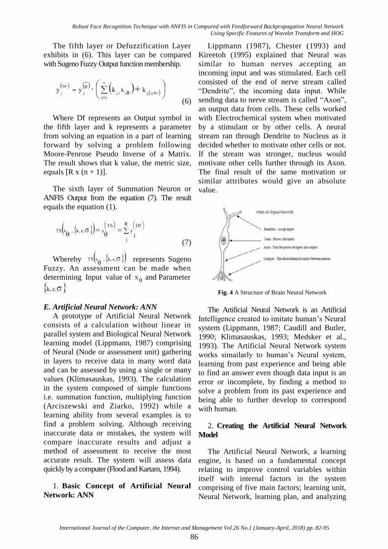
Lippmann (1987), Chester (1993) and

Kireetoh (1995) explained that Neural was

similar to human nerves accepting an

incoming input and was stimulated. Each cell

consisted of the end of nerve stream called

“Dendrite”, the incoming data input. While

sending data to nerve stream is called “Axon”,

an output data from cells. These cells worked

with Electrochemical system when motivated

by a stimulant or by other cells. A neural

stream ran through Dendrite to Nucleus as it

decided whether to motivate other cells or not.

If the stream was stronger, nucleus would

motivate other cells further through its Axon.

The final result of the same motivation or

similar attributes would give an absolute

value.

Fig. 4 A Structure of Brain Neural Network

The Artificial Neural Network is an Artificial

Intelligence created to imitate human’s Neural

system (Lippmann, 1987; Caudill and Butler,

1990; Klimasauskas, 1993; Medsker et al.,

1993). The Artificial Neural Network system

works simailarly to human’s Neural system,

learning from past experience and being able

to find an answer even though data input is an

error or incomplete, by finding a method to

solve a problem from its past experience and

being able to further develop to correspond

with human.

2. Creating the Artificial Neural Network

Model

The Artificial Neural Network, a learning

engine, is based on a fundamental concept

relating to improve control variables within

itself with internal factors in the system

comprising of five main factors; learning unit,

Neural Network, learning plan, and analyzing



87

process (Adeli, 1992). Elazouni et al. (1997).

Elazouni devided a component of Artificial

Neural Network in three stages; 1) design, 2)

creating a model, and 3) testing and finding a

result whereby the design stage is composed

of two parts which are the structural problem

analysis and the problem analysis. However,

creating a model stage will be subdivided into

three steps; 1) selecting data, 2) selecting a

Network model, and 3) teaching and testing a

Network.

3. Data Input

The Artificial Neural Network comprises of

independent variables or data input and

dependent variables or result by selecting

related variables used in the Network (Smith,

1993) in two methods; the first method, data

will be transformed in a suitable format and

the second method is to select data using a

fundamental between predictiveness and

covariance.

Normally, selected independent variables

are able to predict the result if they are related.

On the other hand, if two independent

variables are related the model will be

sensitive and a problem will occur so called

“over fitting and limit generalization”. By this

reason, when selecting data, selection must be

only independent variables that can predict to

receive a result or variables. Those selected

independent variables must not be related.

However, it depends on the Network used to

reduce the samples for teaching and time spent

in learning. The data selection for input should

be suitable because selecting data is an

important factor to create a model (Wu and

Lim, 1993).

4. Hidden Layer

A Hidden Layer is an assessing layer

between an Input Layer and a Result Layer.

Usually, a Hidden layer may have more than

one layer while a Network will be able to

assess a suitable function from more

complicated problems (Lippmann, 1987). The

receiving data from the Hidden Layer will be a

new variable to be sent to a Result Layer or

Variable layer. If Back propagation has less

Hidden Layers, the Network may not find

ways to solve a problem (Karunasekra, 1992).

On the contrary, if there are too many Hidden

Layers the Network will take longer time to

learn(William, 1993).William remarked that

many Hidden Layers would not help the

Network run more efficiently or in other words

Rumelhart (1988), remarked that having too

many Nodes in each layer would make the

Network unable to find the ending point. Too

many Nodes in the Hidden Layers will create a

problem called “Over fitting” where by the

Network will create a new structural model

exceeding a fact from a Noise of data instead

of finding suitable function to make

appropriate Intelligence Analysis correctly

(Smith, 1993). Therefore, to make the Network

most efficient, Nodes in the Hidden Layer

must be determined to be as least as possible

(Khan, Topping and Bahreininejad, 1993)

Berke and Hajela (1991) suggested that a

number of Node in the Hidden Layer should be

between an average sum of Node in Input data

and the Result Layer. Rogers and Ramarsh

(1992) gave an opinion that setting Nodes in

the Hidden Layer should consider the sum of

Node in the Data input Layer and the Result

Layer. Soemardi (1996) remarked that the

number of Node in the Hidden Layer should be

75 percent of Node in the Data input Layer. In

conclusion from the opinion, a number of

Node in the most Hidden Layer should be

equal to the sum of Node in the Data input

Layer and the Result Layer and the least

number of Node should be 75 percent of Nodes

in the Data input Layer or equals to the

average sum of Node in the Data input Layer

and the Result Layer.

5. Weights and Biases

Weights are replaced by numbers to show a

strength to connect each Node being

integrated. The sum of weight input will

improve an assessment in each Node. Weight

is a strength relation (Mathematics) in

connection which will impact the passing of

data through one Layer to another Layer

(Medsker et al., 1993). Usually, weight is

determined and brought into the Network in




88

learning process based on the principle to

ensure that the Network can solve a problem

and reduce the time in learning. For networks,

weight is equal a multiplication of a number of

Node in every connection and the value of

Bias is equal to a sum of a number of Node in

every connection.

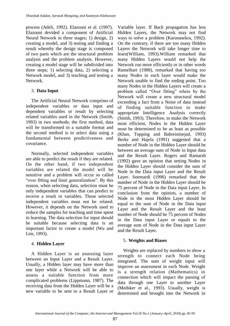
6. Summation and Transfer Function

Summation function is a function to find an

average weight of every connecting Node. The

procedures are to input data in each Node and

to multiply by a weight of every Node and

sum all Nodes together as shown in Fig. 5.

Whereas Transfer function is a relationship

between a level of stimulation within a Node

(N) under conditions: 1) continuous and 2)

value of function Sigmoy will increase when

N increases (Smith, 1993).

Fig. 5 A Working Process in Artificial Neural Network in Sub Nodes

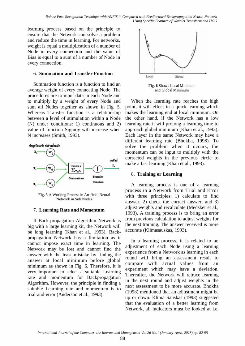
7. Learning Rate and Momentum

If Back-propagation Algorithm Network is

big with a large learning kit, the Network will

be long learning (Khan et al., 1993). Back-

propagation Network has a limitation as it

cannot impose exact time in learning. The

Network may be lost and cannot find the

answer with the least mistake by finding the

answer at local minimum before global

minimum as shown in Fig. 6. Therefore, it is

very important to select a suitable Learning

rate and momentum for Backpropagation

Algorithm. However, the principle in finding a

suitable Learning rate and momentum is to

trial-and-error (Anderson et al., 1993).

Fig. 6 Shows Local Minimum and Global Minimum

When the learning rate reaches the high

point, it will effect in a quick learning which

makes the learning end at local minimum. On

the other hand, if the Network has a low

learning rate it will prolong a learning time to

approach global minimum (Khan et al., 1993).

Each layer in the same Network may have a

different learning rate (Bhokha, 1998). To

solve the problem when it occurs, the

momentum can be input to multiply with the

corrected weights in the previous circle to

make a fast learning (Khan et al., 1993).

8. Training or Learning

A learning process is one of a learning

process in a Network from Trial and Error

with three principles: 1) calculate to find

answer, 2) check the correct answer, and 3)

adjust weights and recalculate (Medsker et al.,

1993). A training process is to bring an error

from previous calculation to adjust weights for

the next training. The answer received is more

accurate (Klimasauskas, 1993).

In a learning process, it is related to an

adjustment of each Node using a learning

experience from a Network as learning in each

round will bring an assessment result to

compare with actual values from an

experiment which may have a deviation.

Thereafter, the Network will retrace learning

in the next round and adjust weights in the

next assessment to be more accurate. Bhokha

(1998) mentioned that an adjustment might be

up or down. Klima Sauskas (1993) suggested

that the evaluation of a better learning from

Network, all indicators must be looked at i.e.



89

mean square error in the Result Layer.

Lippmann (1987) and Smith (1993) mentioned

that the learning process could be divided into

two characteristics;

1) Supervised training comprises of a pair

of input data and the actual result when the

Network starts to learn from the input data and

calculate the result then compare with actual

result to find the deviation to be resent back to

the Network with a weight adjustment for the

Network to calculate a new result with least

deviation.

2) Unsupervised training was discovered by

Kogonen (1984) which is quite different from

a model that simulates a human brain while the

actual result may not be used for a comparison

but would rather use a statistical attribute of a

testing kit to classify in groups after inputting

data. The model will make a possible

assessment in series (Heaton, 2004).

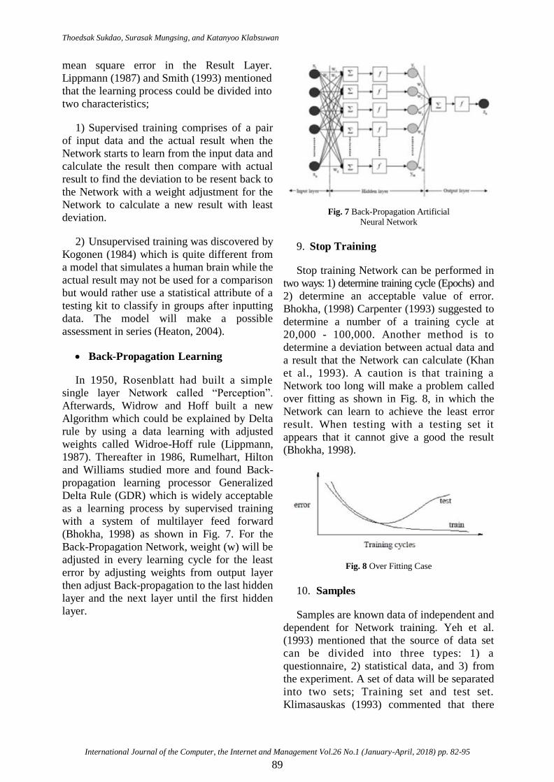
Back-Propagation Learning

In 1950, Rosenblatt had built a simple

single layer Network called “Perception”.

Afterwards, Widrow and Hoff built a new

Algorithm which could be explained by Delta

rule by using a data learning with adjusted

weights called Widroe-Hoff rule (Lippmann,

1987). Thereafter in 1986, Rumelhart, Hilton

and Williams studied more and found Back-

propagation learning processor Generalized

Delta Rule (GDR) which is widely acceptable

as a learning process by supervised training

with a system of multilayer feed forward

(Bhokha, 1998) as shown in Fig. 7. For the

Back-Propagation Network, weight (w) will be

adjusted in every learning cycle for the least

error by adjusting weights from output layer

then adjust Back-propagation to the last hidden

layer and the next layer until the first hidden

layer.

Fig. 7 Back-Propagation Artificial

Neural Network

9. Stop Training

Stop training Network can be performed in

two ways: 1) determine training cycle (Epochs) and

2) determine an acceptable value of error.

Bhokha, (1998) Carpenter (1993) suggested to

determine a number of a training cycle at

20,000 - 100,000. Another method is to

determine a deviation between actual data and

a result that the Network can calculate (Khan

et al., 1993). A caution is that training a

Network too long will make a problem called

over fitting as shown in Fig. 8, in which the

Network can learn to achieve the least error

result. When testing with a testing set it

appears that it cannot give a good the result

(Bhokha, 1998).

Fig. 8 Over Fitting Case

10. Samples

Samples are known data of independent and

dependent for Network training. Yeh et al.

(1993) mentioned that the source of data set

can be divided into three types: 1) a

questionnaire, 2) statistical data, and 3) from

the experiment. A set of data will be separated

into two sets; Training set and test set.

Klimasauskas (1993) commented that there




90

should be at least five test sets for Network

training.

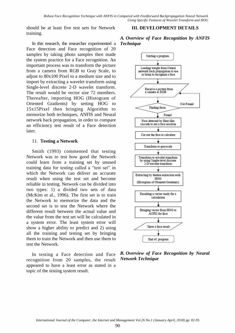
In this research, the researcher experimented a

Face detection and Face recognition of 20

samples by taking photo samples then made

the system practice for a Face recognition. An

important process was to transform the picture

from a camera from RGB to Gray Scale, to

adjust to 80x100 Pixel to a medium size and to

import by extracting a wavelet transform using

Single-level discrete 2-D wavelet transform.

The result would be vector size 72 members.

Thereafter, importing HOG (Histogram of

Oriented Gradients) by setting HOG to

15x15Pixel then bringing Algorithm to

memorize both techniques, ANFIS and Neural

network back propagation, in order to compare

an efficiency test result of a Face detection

later.

11. Testing a Network

Smith (1993) commented that testing

Network was to test how good the Network

could learn from a training set by unused

training data for testing called a “test set” in

which the Network can deliver an accurate

result when using the test set and become

reliable in testing. Network can be divided into

two types: 1) a divided two sets of data

(McKim et al., 1996). The first set is to train

the Network to memorize the data and the

second set is to test the Network where the

different result between the actual value and

the value from the test set will be calculated in

a system error. The least system error will

show a higher ability to predict and 2) using

all the training and testing set by bringing

them to train the Network and then use them to

test the Network.

In testing a Face detection and Face

recognition from 20 samples, the result

appeared to have a least error as stated in a

topic of the testing system result.

III. DEVELOPMENT DETAILS

A. Overview of Face Recognition by ANFIS

Technique

B. Overview of Face Recognition by Neural

Network Technique



91

C. Design and Development

1. Preparing a Picture for Practicing

Receiving a picture as RGB from a camera.

Transforming to grayscale.

Adjusting to a medium size to 80x100.

2. Improving a Picture before Face Detection

Importing wavelet transform by using Single-level discrete 2-D wavelet transform.

The result will be vector size 72 member.

Importing HOG (Histogram of Oriented Gradients) by setting HOG to 15x15.

Bringing the result from HOG to

Algorithm to memorize both techniques.

IV. TESTING AND DISCUSSION

A. Testing for Efficiency to Detect Faces

The Test will be divided into two parts as

follows;

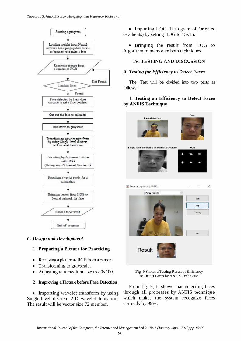
1. Testing an Efficiency to Detect Faces

by ANFIS Technique

Fig. 9 Shows a Testing Result of Efficiency

to Detect Faces by ANFIS Technique

From fig. 9, it shows that detecting faces

through all processes by ANFIS technique

which makes the system recognize faces

correctly by 99%.




92

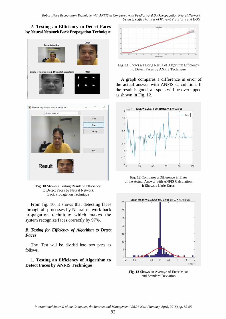
2. Testing an Efficiency to Detect Faces

by Neural Network Back Propagation Technique

Fig. 10 Shows a Testing Result of Efficiency

to Detect Faces by Neural Network Back Propagation Technique

From fig. 10, it shows that detecting faces

through all processes by Neural network back

propagation technique which makes the

system recognize faces correctly by 97%.

B. Testing for Efficiency of Algorithm to Detect

Faces

The Test will be divided into two parts as

follows;

1. Testing an Efficiency of Algorithm to

Detect Faces by ANFIS Technique

Fig. 11 Shows a Testing Result of Algorithm Efficiency

to Detect Faces by ANFIS Technique

A graph compares a difference in error of

the actual answer with ANFIS calculation. If

the result is good, all spots will be overlapped

as shown in Fig. 12.

Fig. 12 Compares a Difference in Error of the Actual Answer with ANFIS Calculation.

It Shows a Little Error.

Fig. 13 Shows an Average of Error Mean and Standard Deviation



93

An average of Error Mean and Standard

Deviation has a small value which results a

little error.

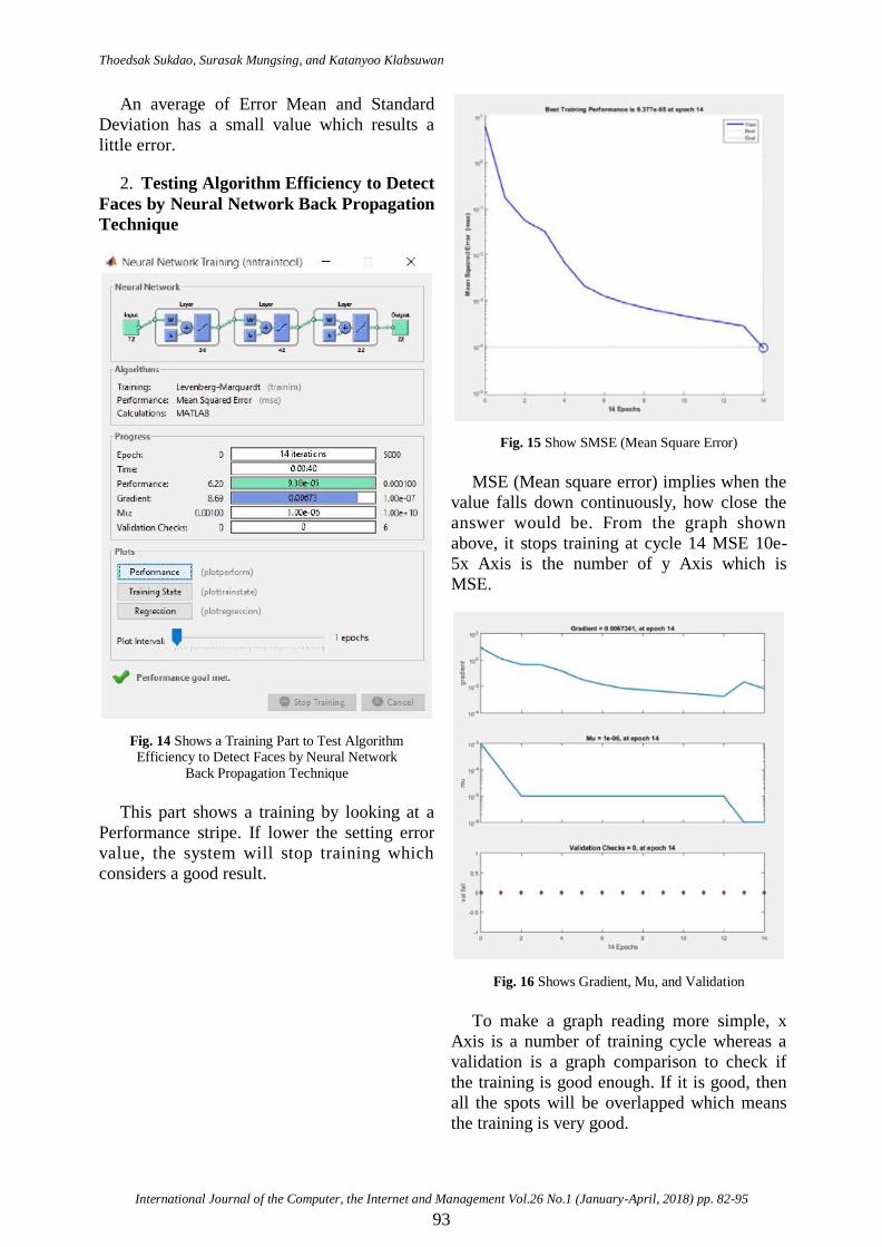
2. Testing Algorithm Efficiency to Detect

Faces by Neural Network Back Propagation

Technique

Fig. 14 Shows a Training Part to Test Algorithm Efficiency to Detect Faces by Neural Network

Back Propagation Technique

This part shows a training by looking at a

Performance stripe. If lower the setting error

value, the system will stop training which

considers a good result.

Fig. 15 Show SMSE (Mean Square Error)

MSE (Mean square error) implies when the

value falls down continuously, how close the

answer would be. From the graph shown

above, it stops training at cycle 14 MSE 10e-

5x Axis is the number of y Axis which is

MSE.

Fig. 16 Shows Gradient, Mu, and Validation

To make a graph reading more simple, x

Axis is a number of training cycle whereas a

validation is a graph comparison to check if

the training is good enough. If it is good, then

all the spots will be overlapped which means

the training is very good.




94

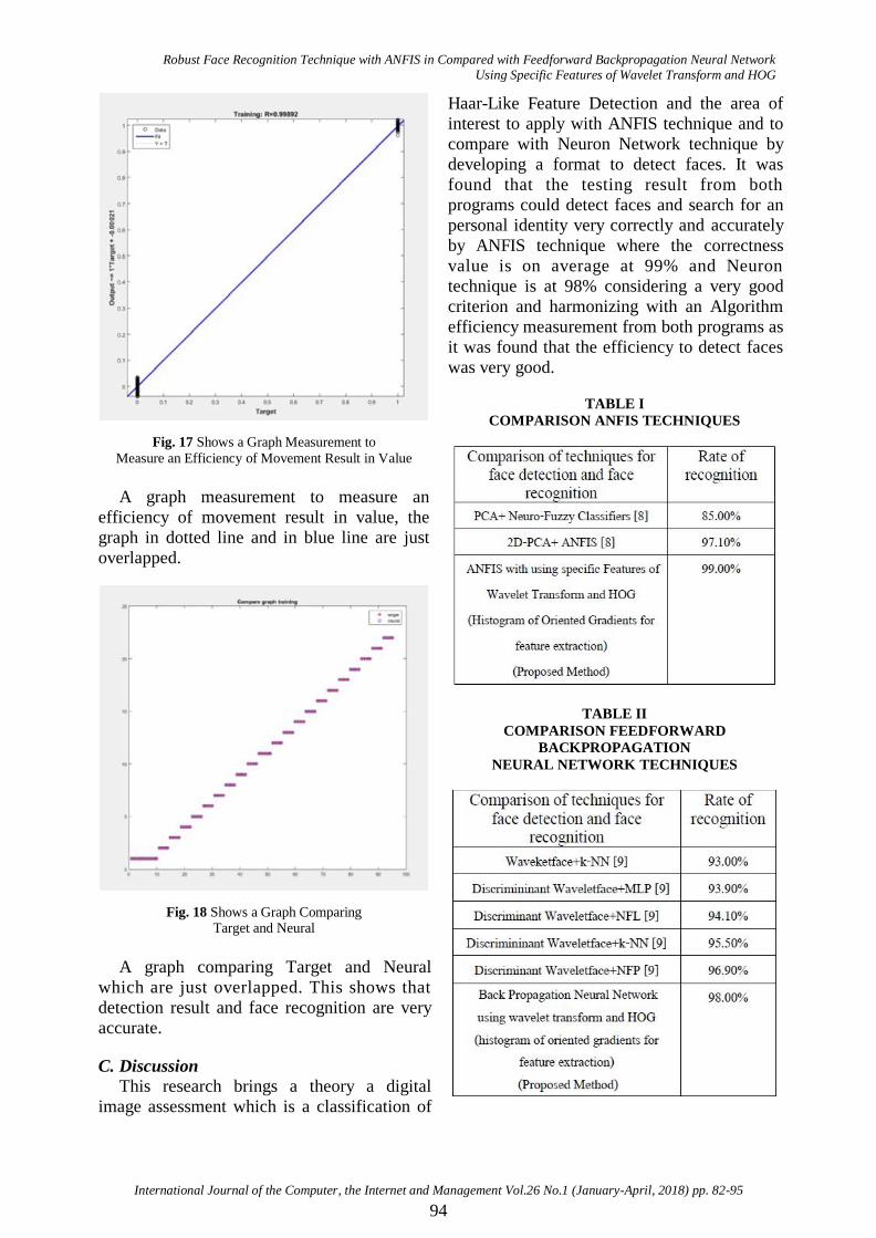
Fig. 17 Shows a Graph Measurement to

Measure an Efficiency of Movement Result in Value

A graph measurement to measure an

efficiency of movement result in value, the

graph in dotted line and in blue line are just

overlapped.

Fig. 18 Shows a Graph Comparing Target and Neural

A graph comparing Target and Neural

which are just overlapped. This shows that

detection result and face recognition are very

accurate.

C. Discussion

This research brings a theory a digital

image assessment which is a classification of

Haar-Like Feature Detection and the area of

interest to apply with ANFIS technique and to

compare with Neuron Network technique by

developing a format to detect faces. It was

found that the testing result from both

programs could detect faces and search for an

personal identity very correctly and accurately

by ANFIS technique where the correctness

value is on average at 99% and Neuron

technique is at 98% considering a very good

criterion and harmonizing with an Algorithm

efficiency measurement from both programs as

it was found that the efficiency to detect faces

was very good.

TABLE I

COMPARISON ANFIS TECHNIQUES

TABLE II

COMPARISON FEEDFORWARD

BACKPROPAGATION

NEURAL NETWORK TECHNIQUES



95

Besides, it was also found that the light and

the distance of a camera had an impact on a

quality of data assessment. However, the result

was satisfactory.

V. CONCLUSION

From the experiment of the face recognition

technique by Haar-Like Feature Detection and

to extract the specific features by Single-level

discrete 2-D wavelet transform then importing

to neural network back propagation, the study

revealed that the rate of face recognition by

ANFIS was correct at 99% and the result of

recognition by neural network back propagation

technique was 98% respectively as it was also

found that detecting face rate was 1% less than

ANFIS technique when extracting the only

specific face feature before detecting a face to

compare with the result.

REFERENCES

(Arranged in the order of citation in the

same fashion as the case of Footnotes.)

[1] Samart, N. and Cheawchanwatana, S.

(2012). “A Face detection area using

model RGBHSV-YcbCr in corporated

with Moorphology”. The graduate research

conference 12th

KhonKaen University,

Thailand, pp. 252-260.

[2] Jain, D., Ilhan, H.T., and Meiyappan, S.

(2003). “A Face detection using Template

Matching”.

<http://www.stanford.edu/class/ee368/Pr

oject_03/Project/slides/ee368group12.ppt>.

[3] Srisuwarat, W. and Phumrin, S. (2008).

“The processing method of a Face

detection module”. The 31st Electrical

Engineering conference (EECON-31),


[4] Adulkasem, S. (2011). “A detection of a

Face Feature of a person; eyes &

mouth”. The Nation Conference on

computing and information Technology,

Thailand, pp. 308.

[5] Sermsub, T. (2012). “A survey research

in Face recognition”. The graduate research

conference 12th

KhonKaen University,


[6] Songsangyos, P. (2005). “Recognizing

and locating positions of various objects”. The

Nation Conference on computing and

information Technology, Thailand, pp.

317.

[7] Sripongsuk, K. “A development of a

system for a personal face recognition”.

<http://www.Development_of_Face_Rec

ognition System_04_04_2011.pdf>.

[8] Shah, H., Kher, R., and Patel, K. (2014).

“Face Recognition Using 2DPCA and

ANFIS Classifier”. Proceedings of Fourth

International Conference on Soft Computing

for Problem Solving, Volume 336 of the

series Advances in Intelligent Systems

and Computing, pp. 1-12.

[9] Chien, J. (2002). “Discriminant Waveletface

and Nearest Feature Classifiers for Face

Recognition”. IEEE Trans, Pattern Analysis

and Machine Intelligence, Vol. 24, pp.

1644-1649.

Documents

Robust Face Recognition Technique with ANFIS in Compared ...ijcim.th.org/past_editions/2018V26N1/26n1Page82.pdf · order to calculate Histogram cell relationship Fig. 2 whereby Pixel