Embed Size (px)
Citation preview

Optimal Robust H∞ Controller for an Integrating Process with Dead Time
CHAPTER 4
ROBUST CONTROLLER DESIGN
4.1 Introduction
The robust controller (H∞
Controller) has been designed and its robustness is checked
with the help of µ synthesis for the unstable processes with dead time. It is important to consider
the various issues like disturbance rejection and the robustness of the controller due to the
uncertainties present in the system. While designing the controller, the weighting functions are
chosen such that the system could meet the performance requirements such as the peak value of
the µ plot should be less than one [12]. The D-K iteration is also used to improve the
performance of the robust controller. Once the D(s) and D-1
(s) were approximated, the plant is
scaled appropriately and the H-infinity design is synthesized for the scaled plant. This procedure
is repeated until the “µ” calculation for robust performance yields a value less than “1” for all
frequencies.
4.2 Design of H-Infinity Controller.
Dan Dai and Roy Smith [11] have discussed about the application of robust control
theory for the cart-spring pendulum system with uncertainties and disturbances. The objective is
to design a controller that meets the specified robust performance criteria. In [12] the authors
have used the “hinfsyn” command to find the controller transfer function by defining all the
input and output parameters. The partitioned matrix of the plant has to be known before using the
70

Optimal Robust H Controller for Unstable Processes with Dead Time
71
“hinfsyn” command. Through the D-K iteration method, plant has been scaled properly and the
controller is found for the synthesized plant. Controller’s robust performance has improved by
using the D-K iteration.
Roy Smith [12]has viewed into the problem of designing a controller to achieve a
performance specification for all plants, G(s), in a set of plants G. Fig. 4.1 represents the generic
synthesis interconnection structure. The lower half of this figure is the same as that for the h-
infinity design procedure. The problem is to find the C(s) such that for all ∆ ε B∆,K(s) stabilizes
Fu(G(s),∆) and ║Fu(Fl(G(s),C(s)),∆║∞ ≤ 1.Unfortunately, this problem is not yet been solved,
except in few special cases. The current approach to this problem, known as D-K iteration,
involves the iterative application of the h-infinity design technique and the upper bound µ
calculation.
Fig 4.1 The generic interconnection structure for synthesis.
Optimal Robust H Controller for Unstable Processes with Dead Time
72
The transfer function model of the distillation column is considered for the design of
robust controller for the unstable process with dead time [1]. Partitioned matrix of the plant is
obtained by considering the performance weight, disturbance weight along with the uncertainties
present in the system Fig. 4.2 which is given by
-------(4.1)
From eq. (4.1), we can define the number of control inputs and number of measurand, which
help to find the H-infinity controller for the plant using “hinfsyn” command.
Fig.4.2 Robust Controller design with weighting functions.

Optimal Robust H Controller for Unstable Processes with Dead Time
73
4.2.1 Robust Control Design Methodology
1. To have the basic idea of designing/selecting lead, lag, lead–lag compensator (It helps
to select the weighting function properly).
2. To model the expected uncertainty into the bound. (│∆│< 1) [41-43]
3. The robust performance of the controller needs to be checked in the presence of the
uncertainty in the system.
4. D-K iteration (D-scaling) method can be used to improve the performance of the
H-infinity controller design [12] for the system.
5. The weighting functions have to be selected based on the systems input requirements.
By understanding the concepts of lead-lag compensator design, the selection of
weighting functions can be made easily.
6. Robust performance can be analyzed in two ways [13]
I. ║│W1S│+│W2T│║∞< 1.
II. Peak value of the µ (D-K iteration) bound should be less than one.
7. Loop shaping method :
a) This section focuses on the tracking of a reference signal.
b) If L denotes the loop transfer function, as L=GC, then the transfer
function from reference input r to tracking error e is given by
S = L1
1 called the sensitivity function, for the specified plant
The condition for therobust performance specification is ║W1S║∞< 1.

Optimal Robust H Controller for Unstable Processes with Dead Time
74
8. The following conditions are used to check for Robust Stability, Nominal Performance,
Robust Performance
The phrases robust stability, nominal performance, and robust performance of the plant.
(i) Nominal Performance: The closed-loop system achieves nominal performance if the
performance objective is satisfied for the nominal plant model, Gnom. In this problem, it is
equivalent to: Nominal Performance ||WP(I + GnomC)–1
||∞< 1
(ii) Robust Stability:The closed-loop system achieves robust stability, if the closedloop system is
internally stable for all of the possible plant models
G .In this problem it is equivalent to a simple
norm test on a particularnominal closed-loop transfer function.
Robust Stability ||WdelCGnom(I + CGnom)–1
||∞< 1
(iii) Robust Performance:The closed-loop system achieves robust performance if theclosed-loop
system is internally stable for all
G , and in addition to that, theperformance objective,||WP(I +
GC)–1
||∞< 1,is satisfied for every
G . The property of robust performance is equivalentto a
structured singular value test (a generalization of the two H∞ norm testsin the previous
conditions) on a particular, nominal closed- loop transferfunction.

Optimal Robust H Controller for Unstable Processes with Dead Time
75
4.3 D-K Iteration for Robust Performance
1. To understand the basic concepts and design of lead-lag compensator (It helps for the
selection the weighting functions).
2. The H-infinity controller has been designed for the integrating process with dead time as
given in [1],by considering various weighting function(Wu, Wd and We).Wu is used to
reduce the error signal at low frequencies to improve tracking, while We limit the control
signal at high frequency to avoid saturation an dynamic range and bandwidth.
3. D-K iteration Algorithm :
The objective is to design a controller which minimizes the upper bound to µ for the
closed loop system ║D(ω)Fl(G(s),C(s)D(ω)-1
║∞.The major problem in doing this is that
the D-Scale that results from µ calculation is in the form frequency by frequency data
and the D-scale required above must be a dynamic system. This requires an
approximation to the upper bound D-Scale in the iteration. Looking into this issuemore
closely, it can be summarized as follows
Initialize procedure withKo(s).
Calculate the resulting closed loopFl(G(s),C(s))
Calculate D scale for µ upper bound
σmax║D(ω)Fl(G(s),C(s)D(ω)-1
║∞ . Approximate the frequency data D(ω),by
D (s) ϵRH∞ , with
D (jω) ≈ D(ω)
Design H∞ Controller for the scaled plant
D (s)G(s)
D-1
(s).

Optimal Robust H Controller for Unstable Processes with Dead Time
76
The notation D(ω) is used to emphasize that the D-Scale arises from frequency by frequency µ
analyses of G(jω)=Fl(G(jω),C(jω)) and therefore is a function of “ω”. Note that it is notthe
frequency response of some transfer function and D(jω) cannot be used as notation. The µ
analysis of the closed loop system is unaffected by the D-Scales. However the H∞ design
problem is strongly affected by scaling. The procedure aims at finding at D such that the upper
bound for the closed loop system is a closed approximation to µ for the closed loop system. At
each frequency, a scaling matrix, D(ω) , can be found such that σmax(D(ω)G(jω)D(ω)-1
) is a
closed upper bound to µ(G(jω)).
Another aspect of “µ” synthesis is to consider the iteration which approaches the optimal
“µ”value, the resulting controllers often have more and more response at high frequencies. The
above discussion used an H∞ controller to initialize the iteration. Actually any stabilizing
controller can be used. In higher order, lightly damped, interconnection structures are used, the
H-infinity design of Ko(s) may be badly conditioned. In such case the software may fail to
generate a controller, or may give controller which doesn’t stabilize the system. A different
controller can be used to get a stable closed loop system, and thereby obtain D scales.
Application of these D scales often results in a better conditioned H-infinity design problem and
the iteration can proceed.
The robust performance difference between the H∞ controller, K0(s), and C(s), can be
dramatic even after a sing D-K iteration. The H∞ problem is sensitive to the relative scaling
between v and w. The D-scale provides the significance better choice of relative scaling for

Optimal Robust H Controller for Unstable Processes with Dead Time
77
closed loop robust performance. Even the application of a constant D scale can have dramatic
benefits [12].
4.4 D-K Iteration results
The stability and robust performance measure of the plant G(s) = 60.0506 se
s
were analyzed and
those are given in the following figures Fig 4.3 to Fig 4.16.
D-K iteration attempts to minimize the quantity ║D(ω)Fl(G(s),C(s)D(ω)-1
║∞ by alternatively
minimizing this expression for the controller C(s) or the “µ” upper bound scaling D, while
holding the other constant. This process is carried out iteratively until a satisfactory controller is
constructed.
Fig 4.3 Bode plot of the plant with and without controller
The frequency roll off is increased with the presence of the controller.
10-5
10-4
10-3
10-2
10-1
100
101
102
-80
-60
-40
-20
0
20
40
60
80
Magnitude (
dB
)
Bode Diagram
Frequency (rad/sec)
Without controller
With controller
Optimal Robust H Controller for Unstable Processes with Dead Time
78
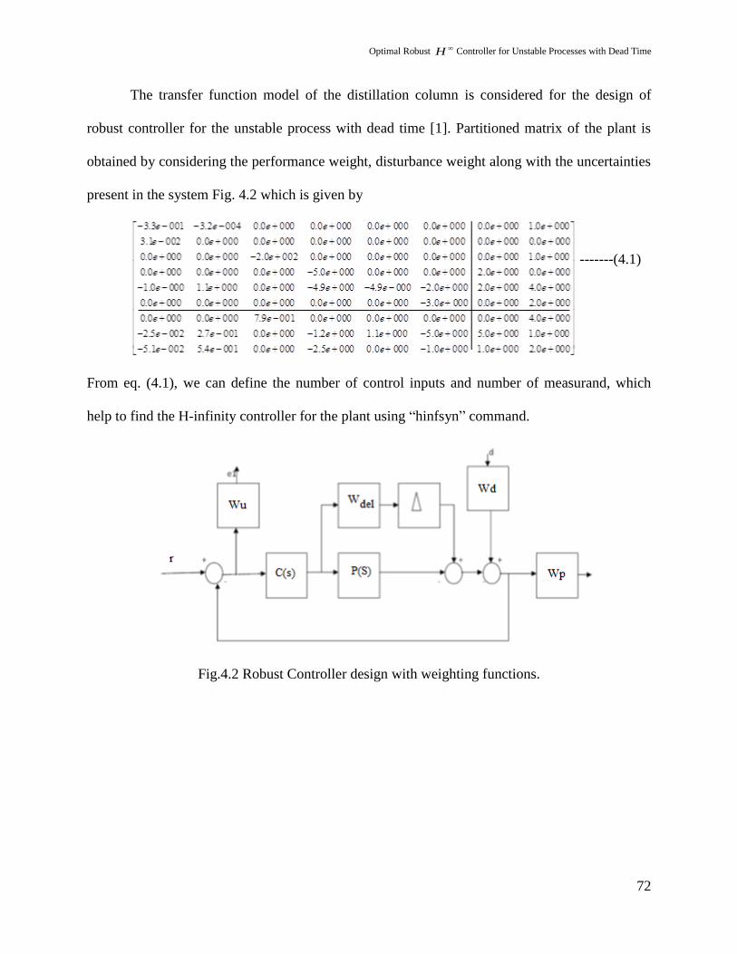
Fig. 4.4 Bode plot of the weighting functions.
Frequency response of the various weighting function is shown in the Figure 4.4.
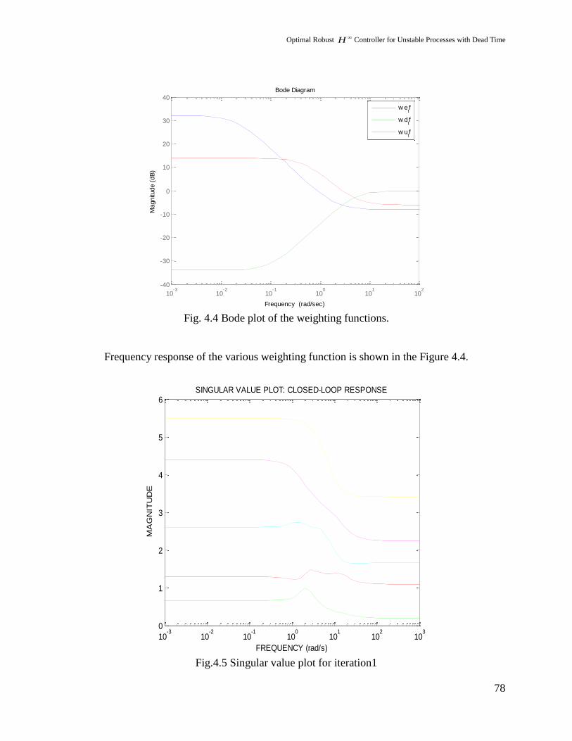
Fig.4.5 Singular value plot for iteration1
10-3
10-2
10-1
100
101
102
-40
-30
-20
-10
0
10
20
30
40
Magnitu
de (
dB
)
Bode Diagram
Frequency (rad/sec)
w etf
w dtf
w utf
10-3
10-2
10-1
100
101
102
103
0
1
2
3
4
5
6SINGULAR VALUE PLOT: CLOSED-LOOP RESPONSE
FREQUENCY (rad/s)
MA
GN
ITU
DE

Optimal Robust H Controller for Unstable Processes with Dead Time
79
Fig.4.6. Mu bound without D Scaling
The peak value of the µ plot is about 4.4 after 1st iteration
Fig.4.7 Mu bound with D-K Scaling
10-3
10-2
10-1
100
101
102
103
2.5
3
3.5
4
4.5CLOSED-LOOP MU: CONTROLLER #1
FREQUENCY (rad/s)
MU
10-3
10-2
10-1
100
101
102
103
2.5
3
3.5
4
4.5MU bnds (solid) and ||D*M*D-1|| (dashed): ITERATION 2
Optimal Robust H Controller for Unstable Processes with Dead Time
80
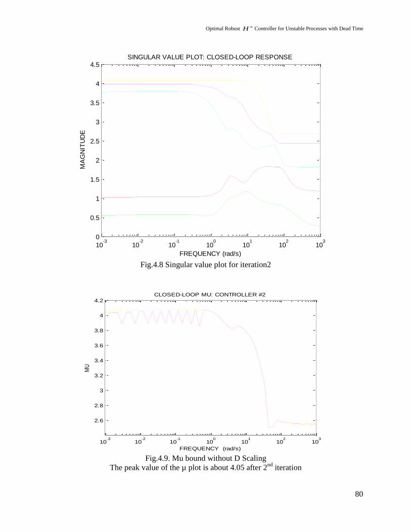
Fig.4.8 Singular value plot for iteration2
Fig.4.9. Mu bound without D Scaling
The peak value of the µ plot is about 4.05 after 2nd
iteration
10-3
10-2
10-1
100
101
102
103
0
0.5
1
1.5
2
2.5
3
3.5
4
4.5SINGULAR VALUE PLOT: CLOSED-LOOP RESPONSE
FREQUENCY (rad/s)
MA
GN
ITU
DE
10-3
10-2
10-1
100
101
102
103
2.6
2.8
3
3.2
3.4
3.6
3.8
4
4.2CLOSED-LOOP MU: CONTROLLER #2
FREQUENCY (rad/s)
MU

Optimal Robust H Controller for Unstable Processes with Dead Time
81
Fig.4.10 Mu bound with D-K Scaling
Fig.4.11 Singular value plot for iteration3
10-3
10-2
10-1
100
101
102
103
2.6
2.8
3
3.2
3.4
3.6
3.8
4
4.2MU bnds (solid) and ||D*M*D-1|| (dashed): ITERATION 3
10-3
10-2
10-1
100
101
102
103
0
0.5
1
1.5
2
2.5
3
3.5
4
4.5SINGULAR VALUE PLOT: CLOSED-LOOP RESPONSE
FREQUENCY (rad/s)
MA
GN
ITU
DE

Optimal Robust H Controller for Unstable Processes with Dead Time
82
Fig.4.12 Mu bound without D Scaling
The peak value of the µ plot is about 4 after 3rd
iteration
Fig.4.13 Mu bound with D-K Scaling
10-3
10-2
10-1
100
101
102
103
2.5
3
3.5
4CLOSED-LOOP MU: CONTROLLER #3
FREQUENCY (rad/s)
MU

Optimal Robust H Controller for Unstable Processes with Dead Time
83
Fig.4.14 Singular value plot for iteration4
Fig.4.15 Mu bound without D Scaling
The peak value of the µ plot is about 3.9 after 4th
iteration.
Since the peak value of “µ” is not less than 1, the robust performance is not ensured for the
controller.
10-3
10-2
10-1
100
101
102
103
0
0.5
1
1.5
2
2.5
3
3.5
4SINGULAR VALUE PLOT: CLOSED-LOOP RESPONSE
FREQUENCY (rad/s)
MA
GN
ITU
DE
10-3
10-2
10-1
100
101
102
103
2.5
3
3.5
4CLOSED-LOOP MU: CONTROLLER #4
FREQUENCY (rad/s)
MU

Optimal Robust H Controller for Unstable Processes with Dead Time
84
4.5Stability Analysis
The condition used to analyze the robust stability was │K(jω)S(jω)│< │1
aW │
Fig.4.16. The robust stability analysis.
4.6 Robust PID controller satisfying the H-Infinity Principles
4.6.1 Introduction
The design of robust controller helps to satisfy the robust stability and robust
performance criteria as given in [13] under the plant parameter changes. Most of the time the
order of the robust controller (H∞) will be of higher order when compared to the process transfer
function. In this thesisan attempt has been made to design the low order controller design (PID
Controller with H-Infinity Principles for aPure Integrating Process with Dead Time (PIPDT)).
The controller design parameters such as Proportional gain, Derivative gain and Integral gain are
fixed using the principle of Hurwitz Criteria. The weighing functions of the system needs to be
selected, based on the low pass or high pass requirements of the input signal and disturbance
rejection. After finding the range of Derivative gain and the Integral gain, by sweeping the
proportional gain, we can find the various set of admissible layers of PID Controller values.

Optimal Robust H Controller for Unstable Processes with Dead Time
85
Finally, the three dimensional plots of the admissible set of PID controller values for the PIPDT
need to be plotted. Once we obtain the admissible set of PID controller settings, that satisfies the
robust performance conditions [13], it can also be easily implemented in the industries as a lower
order H-Infinity controller.
4.6.2.Robust PID Controller Design
Most of the chemical and process industries are encountered with the unstable and higher
order systems. We can model the higher order systems to FOPDT, for the purpose of controller
design. For example, in the study of the distillation column, the resultant FOPDT will have a
very large time constant, which may lead the process to settle after a very long time dead time
instants [1]. For those cases we can treat the model as a pure integrating process for the design of
controller. Once the controller has been designed, the same can be implemented for higher order
systems.
The mathematical model of the distillation column is considered for simulation studies.
Model free PID controller design is more suitable for the integrating process with various
uncertainties. The common problem with the ordinary conventional controller is that, the PID
values which are tuned will give better response only for one particular transfer function. The
tuned controller value may lead to the poor time domain response or unstable output under some
additional uncertainties added into the system. A robust controller may find solution to these
kinds of problems, the only disadvantage with the design of H-Infinity is that the order of the
controller will be very high. In order to reduce the order of the controller and to ensure the robust
performance, an H-Infinity based PID controller [10, 13, 25, 54, 55, 56, ]are proposed for the

Optimal Robust H Controller for Unstable Processes with Dead Time
86
PIPDT processes. Also the admissible set of PID controller which is found using the Hurwitz
Criterion satisfies the robust performance condition. The uncertainty is considered in the form of
dead time in PIPDT process and the PID tuning values are found for uncertain system and
plotted as a 3D plot.
4.6.3 Design Approach
Consider the mathematical model of the distillation column as 60.0506
( )se
G ss
for the
controller design [4, 59-62, 68]. The general structure of the PID controller is given by
2
( )i p dK K s K s
C ss
. Our objective is to find the values ,p iK K and dK using the Hurwitz
Criterion.
The PID values are selected by satisfying the following condition
1] ( , , , )p i ds K K K (4.2)
2] ( , , , , , )p i ds K K K (4.3)
3]1 2( ) ( ) 1W s S W s T
(4.4)
The controller has been designed for the plant with uncertainty, the uncertainty is
considered in the form of various dead time in the process. The perturbed plant with various dead
times are given below (after the pade approximation), for which the controller needs to be
designed.
Case-1: With dead time Td=6sec.
2
0.0506 0.0168( )
0.33
sG s
s s
(4.5)

Optimal Robust H Controller for Unstable Processes with Dead Time
87
Case-2: With dead time Td=4sec.
2
0.0506 0.0253( )
0.5
sG s
s s
(4.6)
Case-3: With dead time Td=2sec.
ss
ssG
0
0506.00506.0)(
2
(4.7)
The root locus plot helps to get the approximate values of Kp for all the three cases.

Optimal Robust H Controller for Unstable Processes with Dead Time
88
Fig.4.17. Root locus plot for Case 1, the maximum value of the gain is 6.63.
Root Locus
Real Axis
Imagin
ary A
xis
-0.4 -0.2 0 0.2 0.4 0.6 0.8 1-0.5
-0.4
-0.3
-0.2
-0.1
0
0.1
0.2
0.3
0.4
0.5
0.220.440.62
0.76
0.85
0.92
0.965
0.992
0.220.440.62
0.76
0.85
0.92
0.965
0.992
0.1
0.2
0.3
0.4
0.5
0.1
0.2
0.3
0.4
0.5
System: s
Gain: 6.63
Pole: 0.00231 + 0.332i
Damping: -0.00695
Overshoot (%): 102
Frequency (rad/sec): 0.332
Optimal Robust H Controller for Unstable Processes with Dead Time
89
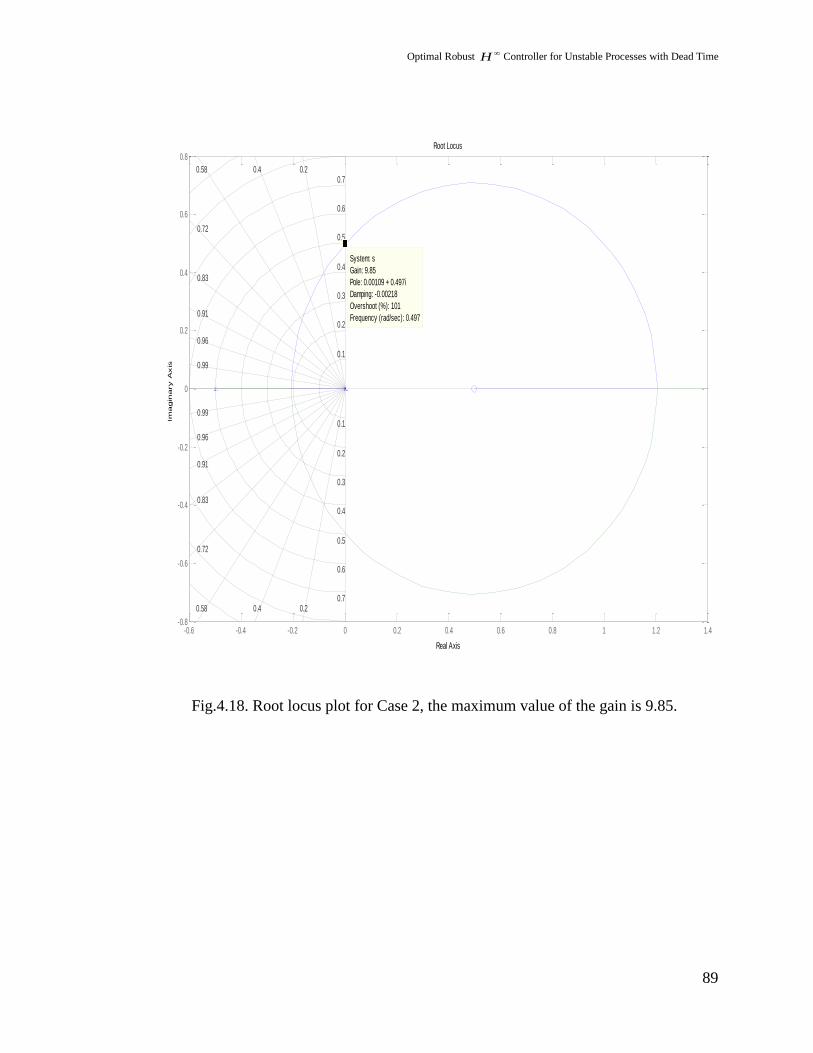
Fig.4.18. Root locus plot for Case 2, the maximum value of the gain is 9.85.
-0.6 -0.4 -0.2 0 0.2 0.4 0.6 0.8 1 1.2 1.4-0.8
-0.6
-0.4
-0.2
0
0.2
0.4
0.6
0.8
0.20.40.58
0.72
0.83
0.91
0.96
0.99
0.20.40.58
0.72
0.83
0.91
0.96
0.99
0.1
0.2
0.3
0.4
0.5
0.6
0.7
0.8
0.1
0.2
0.3
0.4
0.5
0.6
0.7
0.8
System: s
Gain: 9.85
Pole: 0.00109 + 0.497i
Damping: -0.00218
Overshoot (%): 101
Frequency (rad/sec): 0.497
Root Locus
Real Axis
Imagin
ary A
xis

Optimal Robust H Controller for Unstable Processes with Dead Time
90
Fig.4.19.Root locus plot for Case 3, the maximum value of the gain is 19.8.
The weighting functions W1(s) and W2(s) are quite sensitive and should be chosen carefully for
all the three cases based on the frequency inputs of the plants.Let T(s) and S(s) be the
complementary sensitivity function and the sensitivity function respectively.
)()(1
)()()(
sCsG
sCsGsT
(4.8)
)()(1
1)(
sCsGsS
(4.9)
-1 -0.5 0 0.5 1 1.5 2 2.5 3-1.5
-1
-0.5
0
0.5
1
1.5
0.220.42
0.6
0.74
0.84
0.92
0.965
0.99
0.220.42
0.6
0.74
0.84
0.92
0.965
0.99
0.2
0.4
0.6
0.8
1
1.2
1.4
0.2
0.4
0.6
0.8
1
1.2
1.4
System: s
Gain: 19.8
Pole: 0.00359 + 0.996i
Damping: -0.0036
Overshoot (%): 101
Frequency (rad/sec): 0.996
Root Locus
Real Axis
Imagin
ary A
xis

Optimal Robust H Controller for Unstable Processes with Dead Time
91
Also for the case 1, the weighting functions are selected as
5
2)(1
ssW (4.10)
2
15)(2
s
ssW (4.11)
By substituting the proposed control structure C(s) and the plant transfer function P(s) eq. 4.5 in
eq. 4.8 and eq. 4.9 gives the following expressions
3 2
3 2
0.0506 (0.0168 0.0506 ) (0.0168 0.0506 ) 0.0168( )
(1 0.0506 ) (0.333 0.0168 0.0506 ) (0.0168 0.0506 ) 0.0168
d p p i i
d d p i i
Kds K K s K K s KT s
K s K K s Kp K s K
3
3 2
0.333( )
(1 0.0506 ) (0.333 0.0168 0.0506 ) (0.0168 0.0506 ) 0.0168d d p i i
s sS s
K s K K s Kp K s K
Especially, we consider the problem of disturbance rejection for the plant with multiplicative
uncertainty. This problem can be formulated as the following robust performance condition
1|(s)T(s) W| +|(s)S(s) W| 21
This condition can be converted into a simultaneous polynomial stabilization by considering the
following lemma.

Optimal Robust H Controller for Unstable Processes with Dead Time
92
Lemma 1:
Convolute the transfer function of the W1(s) and the transfer function of the Sensitivity
function “S” to form the single transfer function ( )
( )
A s
B s , similarly convolute the W2(s) and
complementary sensitivity function “T” to form the single transfer function ( )
( )
C s
D s
Let
0 11
0 1
...( )( ) ( )
( ) ...
x
x
x
x
a a s a sA sW s S s
B s b b s b s
and
0 12
0 1
...( )( ) ( )
( ) ...
x
x
x
x
c c s c sC sW s T s
D s d d s d s
The transfer function of the( )
( )
A s
B s should be stable and proper rational functions with
and d x not equal to zero. Then,
( ) ( )
1( ) ( )
A s C s
B s D s
If and only if:
a) 1x x
x x
a c
b d
b) ( ) ( ) ( ) ( ) ( ) ( )j jB s D s e A s D s e C s B s is Hurwitz for all θ and ϕ Є [0,2π].
Lemma 2:
For a plant, the control found must satisfy
δ( s,Kp,Ki) is Hurwitz if and only if
( ( , , , ) *( )) ( ( ( ) ( ( ))i p i ds K K K M s n l N s r N s

Optimal Robust H Controller for Unstable Processes with Dead Time
93
The task now is to find the sets of (Kp,Ki,Kd) for which the formula in lemma 2 holds. By
considering the even and odd parts of N(s) and using them to find M*(s), then substitute the
result to find ( , , , ) *( )p i ds K K K M s
Analysis
Using the Lemma 1,
The necessity of condition (b) is established in the following way:
||
| |
||
1x x
x x
a c
b d
( ) ( ) ( ) ( )( ) ( ) ( ) ( ) ( ) ( )
( ) ( )
j j
j je A j D j e C j B j
B s D s e A s D s e C s B sB j D j
( ) ( ) ( ) ( ) ( ) ( )j jB s D s e A j D j e C j B j
( ) ( )
( ) ( )
A j C j
B j D j
0 0 0 00 0
0 0 0 0
( ) ( ) ( ) ( )( ) ( )
( ) ( ) ( ) ( )
A j D j C j B jA j C j
B j D j B j D j
0 0( ) ( )
( ) ( ) ( ) ( )1
( ) ( )
j j
B j D j
e A j D j e C j B j
B j D j
It follows that
( ) ( ) ( ) ( ) ( ) ( )j jB j D j e A j D j e C j B j
Because B(s) and D(s) are Hurwitz, using Rouch’s Theorem we conclude that,

Optimal Robust H Controller for Unstable Processes with Dead Time
94
( ) ( ) ( ) ( ) ( ) ( )j jB s D s e A s D s e C s B s is Hurwitz for all ϴ&Φ Є [0,2π].
Sufficiently proceeding by contradiction we assume that conditions (a) and (b) are true but,
( ) ( )
1( ) ( )
A s C s
B s D s
a) Since ( ) ( )
( ) ( )
A s C s
B s D s is continuous function of ω and
(||
| |
||) |
| |
|
Then there must exist at least one ω0 Є R such that
(( ) ( )
( ) ( )
A s C s
B s D s ) 1x x
x x
a c
b d = 1
Therefore, it implies that there exists ϴ and Φ Є [0,2π] such that
(a) ( ) ( ) ( ) ( ) ( ) ( ) 0j jB s D s e A s D s e C s B s and it obviously contradicts condition
(b). Designing of PID controllers such that the robust performance condition
1|(s)T(s) W| +|(s)S(s) W| 21
holds. Based on lemma 1, The problem of synthesizing PID
controllers for robust performance[9] can be converted into the problem of determining values
of (Kp, Ki, Kd) for which the condition (4.2),(4.3) & (4.4) must hold
Where2( , , , ) ( ) ( ) ( )p i d i p ds K K K sD s K K s K s N s
For condition (4.4) to hold,
|(s)T W| +|(s)SW| 2 1 |
| , Kd must lie in
within the range (-4.9407 , 3.2938 ).
Let :
Optimal Robust H Controller for Unstable Processes with Dead Time
95
2( , , , ) (1 0.0506 (0.333 0.0168 0.0506 ) (0.0168 0.0506 ) 0.0168p i d d p p i is K K K Kd K K s K K s K
5 4( , , , , , ) (1 0.0257844950 ) (8.9713 1.34626 0.025784490 )p i d d d ps K K K K s K K s
3
2
(16.153154 0.23784 1.34626 0.0257844950) (4.42110780 0.2368086
0.23784 1.34626 )
(0.2368086 0.23784 )
0.2368086
d p d
p i
p i
i
K K s K
K K s
K K s
K
After the range of Kd is fixed, the next step is to fix the range of Kp such that the robust
performance condition holds good and also ρ and ψ must be Hurwitz within this range.
Let[ We are defining from [13] ]
N(s)=Ne(s2)+s No(s
2) (4.12)
D(s)=De(s2)+s Do(s
2) (4.13)
Using this decomposition of N(s) and D(s) into even and odd part will simplify the calculation
that should be used for fixing the range of Kp.
Using (4.12) and (4.13), M*(s) can be redefined as
M*(s)=N(-s)= Ne(s2)-s No(s
2)
The closed loop characteristics polynomial is
2( , , , ) ( ) ( ) ( ) ( )p i d i d ps K K K sD s K K s N s K sN s
Let n, m be the degree of ( , , , )p i ds K K K and M*(s) respectively. Multiplying ( , , , )p i ds K K K
by M*(s) and examining the resulting polynomial, we get
( , , , ) *( ) ( ( , , , ) *( )) ( ( , , , ) *( ))dp i p i d p i ds K K K M s l s K K K M s r s K K K M s
= ( ( , , , )) ( ( , , , )) ( ( )) ( ( ))l s Kp Ki Kd r s Kp Ki Kd lN s r N s

Optimal Robust H Controller for Unstable Processes with Dead Time
96
( , , , )p i ds K K K of degree n is Hurwitz if and only if
( ( , , , ))p i dl s K K K n
and
( ( , , , )) 0p i dr s K K K
Now, we consider this theorem
Let 𝜹(s)be a given real polynomial of degree n. then
Moreover, ( , , , )p i ds K K K is Hurwitz if and only if .
Using Lemma 2, the values of Kp, Ki & Kd needs to be found out
2 2 2 2 2
0( , , , ) *( ) [ ( ( ) ( ) ( ) ( ))p i d e e os K K K M s s N s D s D s N s
2 2 2 2 2 2 2 2( )( ( ) ( ) ( ) ( ))] ( ( ) ( )i d e e o o e eK s K N s N s S N s N S s D s N s
2 2 2 2 2 2 2 2( ) ( ) ( ( ) ( ) ( ) ( ))]o o p e e o os D s N s K N s N s s N s N s
Substituting (s=jw):
( , , , ) *( ) ( , , ) ( , )p i d i d ps K K K M s p K K jq K
Where
2
1 2( , , ) ( ) ( ) ( )i d i dp K K p K s K p
1( , ) ( ) ( )p pq K q K q
2 2 2 2 2
1( ) ( ( ) ( ) ( ) ( ))e o e op N D D N
2 2 2 2
2( ) ( ) ( ) ( 2) ( )e e o op N N N N
2 2 2 2 2
1( ) [ ( ) ( ) ( ) ( )]e e o oq D N D N
2 2 2 2 2
2( ) [ ( ) ( ) ( ) ( )e e o oq N N N N
Also define

Optimal Robust H Controller for Unstable Processes with Dead Time
97
After computing the equations above, the next step to is to fix the range kp. This can be done
using root locus ideas as following.
Let
Define
as a function of then find the derivative of
with respect to
(
)
by setting
(
) , then from the real zeros of the equation a corresponding Kp values that
are distinct and finite producing either real breakaway points or a root at the origin can be found
from .
The next step is to find the real root distributions of with respect to the
origin.
The necessary condition for fixing the range of Kp is that q( ,Kp) has at least
{
( )
( ) ( )
} (4.14)
real, nonnegative, distinct roots of odd multiplicity. These ranges of Kp satisfying this condition
are called allowable.
Fixing a value for Kp in within the range and evaluate q( Kp) at this value. The real, non-
negative values, distinct finite zeros of are the zeros of q( ,Kp). Let these zeros be
0= 0< 1< 2< … …. < l-2< l-1
Then we have to construct a sequence of numbers as follows:
{
}
Where 𝜶 Є {-1, 1}
For t= 1,2,3,…, l-1:

Optimal Robust H Controller for Unstable Processes with Dead Time
98
{
}
{
}
With defined in this way, we define the string as the following sequence
of numbers: . This admissible string must satisfy the following condition:
( )
For an admissible string , the set of (Ki,Kd) values can be determined from the following string
of linear inequalities:
For which M*(j t)≠0.
This procedure has to be repeated for all admissible strings to obtain the corresponding
admissible (Ki,Kd) sets. The set of all stabilizing (Ki,Kd) values corresponding to the fixed Kp is
then given by
Now we apply this procedure to determine the admissible set of (Kp,Ki,Kd) values. First, let’s
consider the transfer function in case 1.
N(s) and D(s) can be decomposed into even odd parts as following:
* 2 4 2
2 3 3
( , , , ) ( ) 0.0055944 0.0506 ( )
(0.00028224 0.00256036 ) 0.0336498 (0.00028224 0.00256036 )
p i d i d
p
s K K K M s s s K s K
s s K a s

Optimal Robust H Controller for Unstable Processes with Dead Time
99
Evaluating the above equation at s=j :
* 2 4 2 2) 0.0055944 0.0506 ( )(0.00028224 0.( , , , 002560) 3( 6 )i dp i d K Ks K K K M j
3 3(0.00028224( 0.033649 0.002560368 ))j Kp
* 2
1 2 1 2, , , ) ( ) [ ( ) ( ) ( )]( [ ( ) ( )]p i d i d pK K K M j p K K p j q K qj
P1( ), P2( ), q1( ) and q2( ) are found to be:
2 4
2
2
3
1
1
3
2
) 0.0055944 0.0506
( ) (0.00028224 0.00256036 )
( ) 0.0336498
( ) 0.00028224 0.00256036
(
P
q
q
P
q(ω,Kp) can be written in the q( ,Kp)= [ U( ) + Kp V( ) ] form as:
2 2, ) [ 0.0336498 (0.00028224 0.0( 0256036 )]pKq Kp
Where
2
2
) 0.0336498
( ) 0.00028224 0.002
(
56036
U
V
Let
2
2
( 0.00028224 0.00256036
( 0.03364
)
) 98
V
U
2 2
( 0.00001899463910
( ( 0.0336498
)
) )
d V
d U
2 2
0.000018994639100
( 0.0336498 )
(4.15)

Optimal Robust H Controller for Unstable Processes with Dead Time
100
The only real zero eq. (4.15) is =0. Substituting this value in , the
corresponding value w is Kp =0. This gives that the range of Kp can be:
(-∞,0] or [0,∞). Examining the distribution of the roots for Kp will give a more accurate range
for Kp.
Since n+m=4 (even), there must be at least ( )
real, non-negative distinct finite
zeros in the range of Kp. In this case there should be at least
. By choosing any
arbitrary value for Kp in each range, the exact range of Kp can be determined. For this case in our
hand the range of Kp is [0, 13.115].
Taken any arbitrary value for Kp in within the specified range, for instance let Kp =6.5, and
substituting the value in q( ,Kp)gives:
3,6.5) 0.017007460 0.001834 0( 56q
The real zeros of q( , 6.5) with odd multiplicity are ω0=0 and ω1=0.32843. Also define 2=∞.
The next step is to find the admissible strings
Define
2 4
1 2 2
( 0.0055944 0.0506 )( )
(1 )P
Since M*(s) has no zero at the origin and M*(j ωt)≠0 for t=, =𝜶. also will have the value of
𝜶 because n+m is even number.
Since m+n=4, which is even, and M*(s) has no jω-axis roots, then the set A(6.5) becomes
{
}
Since ( ) ( ) and , then
every admissible string must satisfy the condition
Optimal Robust H Controller for Unstable Processes with Dead Time
101
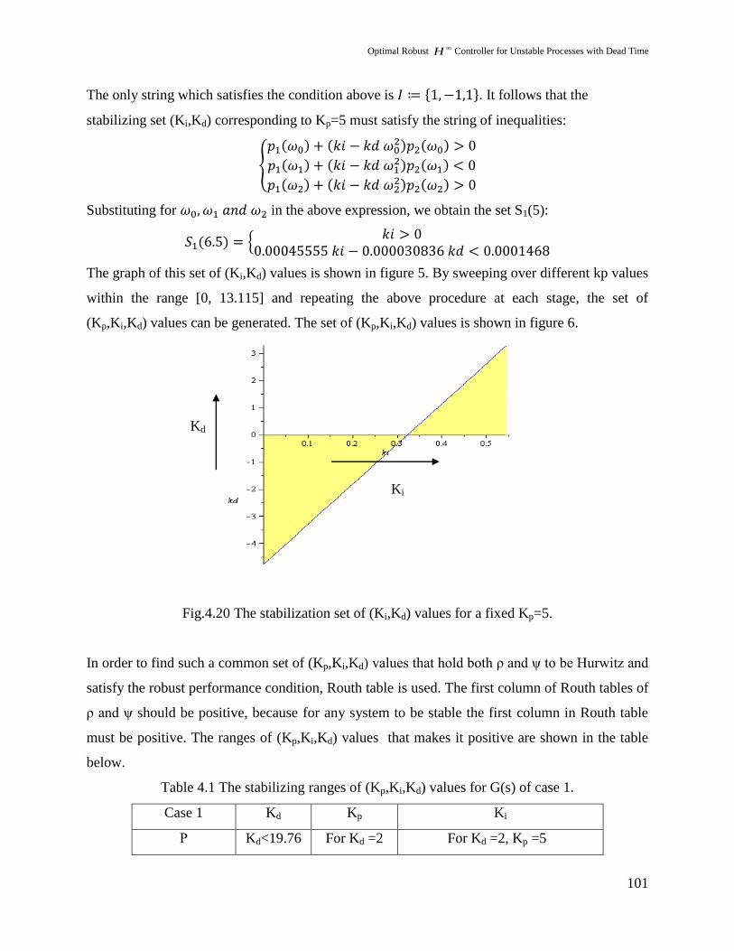
The only string which satisfies the condition above is . It follows that the
stabilizing set (Ki,Kd) corresponding to Kp=5 must satisfy the string of inequalities:
{
Substituting for in the above expression, we obtain the set S1(5):
{
The graph of this set of (Ki,Kd) values is shown in figure 5. By sweeping over different kp values
within the range [0, 13.115] and repeating the above procedure at each stage, the set of
(Kp,Ki,Kd) values can be generated. The set of (Kp,Ki,Kd) values is shown in figure 6.
Fig.4.20 The stabilization set of (Ki,Kd) values for a fixed Kp=5.
In order to find such a common set of (Kp,Ki,Kd) values that hold both ρ and ψ to be Hurwitz and
satisfy the robust performance condition, Routh table is used. The first column of Routh tables of
ρ and ψ should be positive, because for any system to be stable the first column in Routh table
must be positive. The ranges of (Kp,Ki,Kd) values that makes it positive are shown in the table
below.
Table 4.1 The stabilizing ranges of (Kp,Ki,Kd) values for G(s) of case 1.
Case 1 Kd Kp Ki
Ρ Kd<19.76 For Kd =2 For Kd =2, Kp =5
Kd
Ki

Optimal Robust H Controller for Unstable Processes with Dead Time
102
Kp<7.24 0 <Ki< 0.458
Ψ Kd< 3.878 For Kd = 1.5
Kp<26.96
For Kd =1.5, Kp =5
0 <Ki< 77.433
But in order to find a common set of values that satisfied both ρ and ψ and also satisfied the
robust performance condition, the values in the above table have to be modified slightly. One of
the sets that can satisfy the three conditions is in the table below:
Table 4.2 Optimal robust set of (Kp,Ki,Kd) values.
Kd Kp Ki
Case 1 0.5 5 0.2
Note: These are the common values of Kp,Ki and Kd which are satisfying the condition ρ and ψ.
Then, values obtained were substituted in the original equations of ρ and ψ to ensure they will
make the system stable. Table 4.3 &4.4 below shows the first column of ψ and ρ with the values
of (Kp,Ki,Kd) respectively.
Table 4.3Routh table for the condition 2 (Eq. 4.3) - ( , , , , , )p i ds K K K
Routh-Hurwitz: 1st Column is TF Zeros are
s5: 0.87108 -6.4888
s4:7.0089 -1.2726
s3:8.8684 -0.11902-0.35566i
s2: 2.1875 -0.11902+0.35566i
s1:0.93858 -0.046809
s0:0.047362
Table 4.4. Routh table for the condition 1 (Eq. 4.2) – ( , , , )p i ds K K K
Routh-Hurwitz: 1st Column is TF Zeros are
s3:0.9747 -0.021974-0.27067i
s2: 0.0884 -0.021974+0.27067i
s1:0.036833 -0.046746
s0:0.00336

Optimal Robust H Controller for Unstable Processes with Dead Time
103
From Table 4.3 and 4.4 above that the system is completely stable for the set of (Kp,Ki,Kd)
values. All the zeros of ρ and ψ are in the left side of the plane. By sweeping over different
Kpvalues within the interval [0, 13.115) and repeating the above procedure at each stage, the set
of stabilizing (Kp,Ki,Kd) values can be generated.
Fig.4.21. The stabilizing set of (Kp,Ki,Kd) values.
The design of the Robust PID controller satisfying the robust performance for case1 was
completed. The same procedure is to be applied for the other cases. The resulting stabilization set
of (Ki,Kd) and the 3D stabilizing set of (Kp,Ki,Kd) are shown for the case 2 (Plant with
uncertainty) transfer function.
For CASE 2 Transfer Function:
For the plant transfer function of case 2, ρ and ψ equations are as follow:
3 2( , , , ) (1 0.0506 ) (0.5 0.0253 0.0506 ) (0.0253 0.0506 )p i d d d p p is K K K K s K K s K K s
0.0253 iK
0.1
0.2
0.3
0.4
0.5
0.4 0.6 0.8 1 1.2 1.4 1.6 1.8 2
5
5.05
5.1
5.15
5.2
5.25
5.3
5.35
5.4
5.45
5.5
kp
kd
ki
Kp
Kd
Ki

Optimal Robust H Controller for Unstable Processes with Dead Time
104
5 4( , , , ) ( 0.257844950 1) ( 1.30295 0.257844950 9.138)p i d d d ps K K K K s K K s
3( 1.30295 0.002692 0.257844950 17.59575)p d iK K K s
2( 1.30295 0.356622475 0.002692 6.6383)i d pK K K s
(0.35662247 0.002692 ) 0.356622475p i iK K s K
4.7 Robust Performance Condition
For the robust performance condition to be hold:
| |
||
For this condition to be hold, Kd must lies in the range (-4.9407, 3.2938).
Ki
Fig.4.22. The stabilizing set of (Ki,Kd) values when Kp =6.
Table 4.5 The ranges of (Kp,Ki,Kd) values for G(s) of case 2.
Case 2 Kd Kp Ki
Ρ Kd<19.76 For Kd =2
Kp<10.88
For Kd =2, Kp =6
0< Ki<1.062
Ψ Kd<3.878 For Kd =2
Kp<25.334
For Kd =2, Kp =6
0< Ki<69.07
Kd

Optimal Robust H Controller for Unstable Processes with Dead Time
105
Table 4.6.Checked set of (Kp,Ki,Kd) values.
Kd Kp Ki
Case 1 0.5 6 0.5
Fig.4.23. Admissible set of PID controller values for the case2.
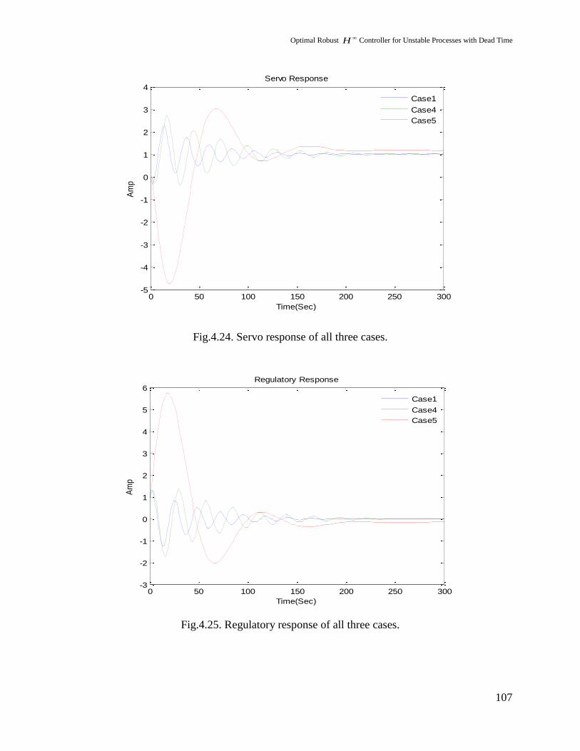
4.8Analysis of Various Combination of Pade Approximation
The plant delay function is approximated to a rational transfer function using different
Pade approximations. The plant transfer function is considered with different approximations of
6se. In case 4, first order Pade approximation in numerator and second order Pade
approximation in the denominator is considered. In case 5, approximated first order in the
numerator (( 1 0a s a )) which is obtained by comparing the magnitude of “S” and “T” of the
higher order controller and the and second order Pade approximation in the denominator is
considered for the analysis. The analysis of various combination of PADE approximation has
been carried out to check whether there is any improvement in the time domain response.
0
0.2
0.4
0.6
0.8
1
0.2 0.4 0.6 0.8 1 1.2 1.4 1.6 1.8
6
6.05
6.1
6.15
6.2
6.25
6.3
6.35
6.4
6.45
6.5kp
kd
ki
Kp
Kd Ki

Optimal Robust H Controller for Unstable Processes with Dead Time
106
Case 4:
60.0506( ) sG s e
s
0.0506 1
2
st
nds Order Pade approximation of
6se
2
0.0506 0.333
0.333
s
s s s
Thus, case 4 transfer function is:
3 2
0.0506 0.0169( )
0.333
sG s
s s
Case 5:
60.0506( ) sG s e
s
1 0
2
0.0506
0.333
a s a
s s s
Thus, case 5 transfer function is:
3 2
1.6955 0.0169( )
0.333
sG s
s s s
By designing the robust PID controller for the Case 4 and Case 5 transfer functions the following
servo and regulatory responses are obtained.
(5.19)
(5.20)
Optimal Robust H Controller for Unstable Processes with Dead Time
107
Fig.4.24. Servo response of all three cases.
Fig.4.25. Regulatory response of all three cases.
0 50 100 150 200 250 300-5
-4
-3
-2
-1
0
1
2
3
4
Time(Sec)
Am
p
Servo Response
Case1
Case4
Case5
0 50 100 150 200 250 300-3
-2
-1
0
1
2
3
4
5
6
Time(Sec)
Am
p
Regulatory Response
Case1
Case4
Case5

Optimal Robust H Controller for Unstable Processes with Dead Time
108
It is observed that the first order PADE approximation gives the better result for the servo and
regulatory response when compared to the other combination of PADE approximation.
4.9 Chapter Conclusion:
Robust controller has been designed for the unstable process with uncertainty. The
analysis of robust performance has been done using µ synthesis (D-K scaling). The weighing
functions have to be adjusted to minimize the peak of the µ plot to be less than one, to maintain
the robust performance of the system. After finding the uncertainty del(∆), the weighing function
for the uncertainty has to be selected as a covering function of the magnitude plot of the del(∆),
to assure the robust stability.The controller bandwidth has been increased with the perturbed
system to maintain the controller stability. When analyzing the robust stability criteria with
respect to bode magnitude plot, it does not hold in the frequency range between 0.00008 rad/sec
to 1.2 rad/sec as shown in Fig.4.16. Therefore the controller is not robustly stable with respect to
the additive uncertainty set. Also the order of the resultant robust controller is found to be
seventh order controller.
In this chapter the robust controller has been designed using the µ synthesis has resulted
with the higher order controller and it finds difficulty in the real time implementation. The need
is to reduce the order of the robust controller and also by preserving the H-Infinity principles.
This leads to the design of robust PID controller.The admissible sets of robust PID controller
values have been found using the Hurwitz criterion for the Pure Integrating Process with dead
time. The PID Controller values obtained satisfy the robust performance condition for the
system. The Controller has been designed for the plant with and without uncertainty in the dead

Optimal Robust H Controller for Unstable Processes with Dead Time
109
time and also the admissible set of 3D plot has been plotted.From the obtained admissible set of
PID values, the narrowed down values of controller parameters need to be identified which will
give the good time domain specifications.
Fig. 4.17, Fig. 4.18 and Fig. 4.19 shows the open loop gain of the cases (1),(2) and (3).
Fig. 4.20 and Fig. 4.22 shows the range of Ki&Kd of Case(1) and Case(2) for the fixed
value of Kp
Fig.4.21 and Fig. 4.23 shows the 3D plot of the admissible set of Robust PID values.
******