Control of Uncertain Nonlinear Systems Using Ellipsoidal Reachability Calculus

Control of Uncertain Nonlinear SystemsUsing Ellipsoidal Reachability Calculus

Leonhard Asselborn Dominic Groß Olaf Stursberg

Institute of Control and System TheoryUniversity of Kassel

[email protected]

[email protected]

[email protected]

www.control.eecs.uni-kassel.de

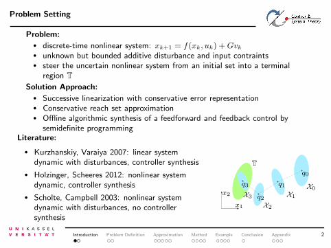
Problem Setting

Problem:• discrete-time nonlinear system: xk+1 = f(xk, uk) +Gvk• unknown but bounded additive disturbance and input contraints• steer the uncertain nonlinear system from an initial set into a terminal

region TSolution Approach:

• Successive linearization with conservative error representation• Conservative reach set approximation• Offline algorithmic synthesis of a feedforward and feedback control by

semidefinite programmingLiterature:

• Kurzhanskiy, Varaiya 2007: linear systemdynamic with disturbances, controller synthesis

• Holzinger, Scheeres 2012: nonlinear systemdynamic, controller synthesis

• Scholte, Campbell 2003: nonlinear systemdynamic with disturbances, no controllersynthesis

X0

X1

X2

X3x2

x1

Tq0

q1

q2

q3

Introduction Problem Definition Approximation Method Example Conclusion Appendix 2

Reach Set Computation - Basics

1. Set representation:Ellipsoid: E = ε(q,Q) =

{x ∈ Rn|(x− q)TQ−1(x− q) ≤ 1

},

Q = QT > 0, q ∈ Rn

Polytope: P = {x ∈ Rn | Kx ≤ b,K ∈ Rnp×n, b ∈ Rnp}.

2. Dynamical system:

xk+1 = f(xk, uk) +Gvk, (1)

x0 ∈ X0 = ε(q0, Q0) ⊂ Rn, (2)

uk ∈ U = {u ∈ Rm | Ruk ≤ b},

vk ∈ V = ε(0,Σ) ⊆ Rn

3. One-step reachable set:

Xk+1 = {x | xk ∈ Xk, uk ∈ U , vk ∈ V : xk+1 = f(xk, uk) +Gvk}

= F (Xk,U)⊕GV (3)

⊕: Minkowski addition.


Problem Definition

Problem 1

Determine a control law uk = κ(xk, k), for which it holds that:

uk ∈ U ∀ k ∈ {0, 1, . . . , N − 1}, N ∈ N, xk ∈ Xk

and that it stabilizes the nonlinear system from an initial set X0 = ε(q0, Q0) ina finite number N of time steps into an ellipsoidal terminal set T = ε(0, T )which is parametrized by T ∈ Rn×n and is centered in the origin 0:

∃ N ≥ 0 : Xk+1 = F (Xk, Uk)⊕GV

XN ⊆ T = ε(0, T ), k ∈ {0, 1, . . . , N − 1}


Preliminaries for Solution

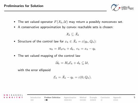
• The set valued operator F (Xk,U) may return a possibly nonconvex set.

• A conservative approximation by convex reachable sets is chosen:

Xk ⊆ Xk

• Structure of the control law for xk ∈ Xk = ε(qk, Qk):

uk = Hkek + dk, ek = xk − qk

• The set valued mapping of the control law

Uk = HkEk + dk ⊆ U ,

with the error ellipsoid

Ek = Xk − qk = ε(0, Qk).


Local Conservative Linearization of the Dynamics (1)

• First order Taylor series expansion with ξk = [xk, uk]T and ξk = [qk, p]

T :

∃z ∈{αξk + (1− α)ξk | α ∈ [0, 1]

}:

f(xk, uk) = f(ξk) +∂f(ξk)

∂ξk

∣∣∣∣ξk=ξk

(ξk − ξk) + L(ξk, z)

• Representation of the nonlinear dynamics with the error term L(ξk, z):

xk+1 ∈ Ak(xk − xk) +Bk(uk − uk) + L(ξk, z) + f(xk, uk) +Gvk


Local Conservative Linearization of the Dynamics (2)

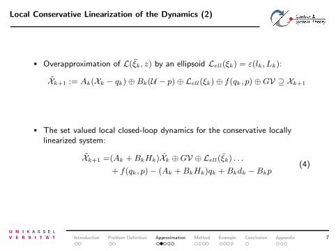
• Overapproximation of L(ξk, z) by an ellipsoid Lell(ξk) = ε(lk, Lk):

Xk+1 := Ak(Xk − qk)⊕Bk(U − p)⊕ Lell(ξk)⊕ f(qk, p)⊕GV ⊇ Xk+1

• The set valued local closed-loop dynamics for the conservative locallylinearized system:

Xk+1 =(Ak +BkHk)Xk ⊕GV ⊕ Lell(ξk) . . .

+ f(qk, p)− (Ak +BkHk)qk +Bkdk −Bkp(4)


Ellipsoidal Calculus

Affine transformation of an ellipsoid ε(q,Q) by A ∈ Rn×n and b ∈ Rn×1 to anellipsoid:

A · ε(q,Q) + b = ε(A · q + b, AQAT )

The Minowski sum Xk+1 of a set of ellipsoids is in general not an ellipsoid, butit can be tightly enclosed by an ellipsoid Xk+1:

Xk ⊆ Xk ⊆ Xk

i.e. Xk is an over approximation of the exact reachable set Xk.

XkXk

Xk


Problem Reformulation (1)

Effect of the chosen control law:

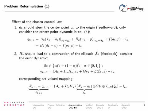
1. dk should steer the center point qk to the origin (feedforward); onlyconsider the center point dynamic in eq. (4):

qk+1 = Ak(xk − qk)|xk=qk+ Bk(uk − p)|

uk=dk+ f(qk, p) + lk

= Bk(dk − p) + f(qk, p) + lk

2. Hk should lead to a contraction of the ellipsoid Xk (feedback); considerthe error dynamic:

∃z ∈{αξk + (1− α)ξk | α ∈ [0, 1]

}:

ek+1 = (Ak +BkHk)ek +Gvk + L(ξk, z)− lk.

corresponding set-valued mapping:

Xk+1 − qk+1︸︷︷︸

Ek+1

= (Ak +BkHk) (Xk − qk)︸︷︷︸

Ek

⊕GV ⊕ Lell(ξk)− lk,


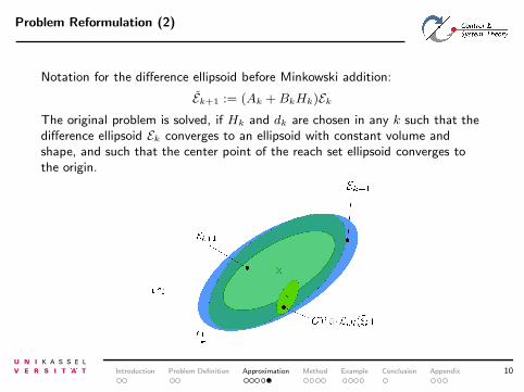
Problem Reformulation (2)

Notation for the difference ellipsoid before Minkowski addition:

Ek+1 := (Ak +BkHk)Ek

The original problem is solved, if Hk and dk are chosen in any k such that thedifference ellipsoid Ek converges to an ellipsoid with constant volume andshape, and such that the center point of the reach set ellipsoid converges tothe origin.


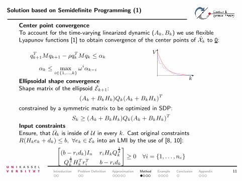
Solution based on Semidefinite Programming (1)

Center point convergenceTo account for the time-varying linearized dynamic (Ak, Bk) we use flexibleLyapunov functions [1] to obtain convergence of the center points of Xk to 0:

qTk+1Mqk+1 − ρq

Tk Mqk ≤ αk

αk ≤ maxi∈{1,...,k}

ωiαk−i

V

kEllipsoidal shape convergenceShape matrix of the ellipsoid Ek+1:

(Ak +BkHk)Qk(Ak +BkHk)T

constrained by a symmetric matrix to be optimized in SDP:

Sk ≥ (Ak +BkHk)Qk(Ak +BkHk)T

Input constraintsEnsure, that Uk is inside of U in every k. Cast original constraintsR(Hkek + dk) ≤ b, ∀ek ∈ Ek into an LMI by the use of [8, 10]:

[

(b− ridk)In riHkQ12k

Q12k H

Tk rTi b− ridk

]

≥ 0 ∀i = {1, . . . , nc}


Solution based on Semidefinite Programming (2)

Semidefinite programm to be solved in any k:

minSk,Hk,dk,αk

trace(Sk) (5)

s. t. :

center point convergence:

qTk+1Mqk+1 − ρqTk Mqk ≤ αk

qk+1 = Bk(dk − p) + f(qk, p) + lk

αk ≤ maxi∈{1,...,k} ωiαk−i

ellipsoidal shape convergence:

trace(Sk) ≤ trace(Qk)[

Sk (Ak +BkHk)T

(Ak +BkHk) Q−1

k

]

≥ 0

input constraints:

(b− ridk)In riHkQ

12k

Q12k H

Tk rTi b− ridk

≥ 0, ∀i = {1, . . . , nc}.


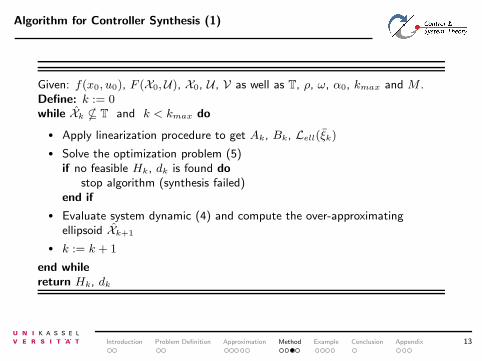
Algorithm for Controller Synthesis (1)

Given: f(x0, u0), F (X0,U), X0, U , V as well as T, ρ, ω, α0, kmax and M .Define: k := 0while Xk * T and k < kmax do

• Apply linearization procedure to get Ak, Bk, Lell(ξk)

• Solve the optimization problem (5)if no feasible Hk, dk is found do

stop algorithm (synthesis failed)end if

• Evaluate system dynamic (4) and compute the over-approximatingellipsoid Xk+1

• k := k + 1

end whilereturn Hk, dk


Algorithm for Controller Synthesis (2)

Lemma 1

If the control algorithm terminates with Xk ⊆ T, k ≤ kmax, the originalproblem is successfully solved and a control law (5) exists which steers theinitial state x0 ∈ X0 into the target set T in N steps for any possibledisturbance vk ∈ V. Furthermore, the input constraint uk ∈ U holds for all0 < k < N , and the center point qk of the reach set Xk asymptoticallyconverges to the origin.

Proof (sketch):• Successful termination of the control algorithm implies that XN ∈ T and

consequently xN ∈ XN ⊆ T holds for all initial states x0 ∈ X0 and alldisturbances vk ∈ V.

• By construction xk ∈ Xk implies that ek ∈ Ek. It follows, that the inputconstraint uk ∈ U holds at each time step, if uk = Hkek + dk ∈ U holdsfor all ek ∈ Ek.

• The use of flexible Lyapunov functions imply that V (xk) = qTk Mqk can beused to ensure asymptotic convergence of the center point qk of Xk (cf.Lemma III.4 in [1]) over the considered horizon N . �


Control of a Three-Tank-System: Dynamic Model

• state: height of fluid inside each tank

• input: valve for in- and outflow with nonlinear characteristic curve

• disturbance: additive measurement uncertainty

• task: fill empty tank system to reference height

System:


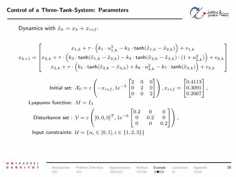
Control of a Three-Tank-System: Parameters

Dynamics with xk = xk + xref :

xk+1 =

x1,k + τ ·(

k1 · u21,k

− k2 · tanh(x1,k − x2,k))

+ v1,k

x2,k + τ ·(

k3 · tanh(x1,k − x2,k) − k4 · tanh(x2,k − x3,k) · (1 + u22,k

))

+ v2,k

x3,k + τ ·(

k5 · tanh(x2,k − x3,k) + k6 · u23,k

− k7 · tanh(x3,k))

+ v3,k

Initial set: X0 = ε

−xref , 1e−3

2 0 00 2 00 0 2

, xref =

0.41130.30910.2067

,

Lyapunov function: M = I3

Disturbance set : V = ε

[0, 0, 0]T , 1e−6

0.2 0 00 0.2 00 0 0.2

,

Input constraints: U = {ui ∈ [0, 1], i ∈ {1, 2, 3}}


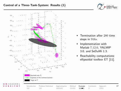
Control of a Three-Tank-System: Results (1)

Target set T

Trajectory of the nonlinear dynamic

Reachable sets Xk

x3

x2

x1

−0.5

0

0.5

−0.4−0.2

00.2

0.4

−0.4

−0.3

−0.2

−0.1

0

0.1

0.2

0.3

0.4

• Termination after 280 timesteps in 916s.

• Implementation withMatlab 7.12.0, YALMIP3.0, and SeDuMi 1.3.

• Reachability computations:ellipsoidal toolbox ET [11].


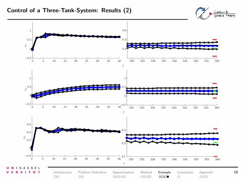
Control of a Three-Tank-System: Results (2)

t

t

t

x3

x2

x1

520 525 530 535 540 545 550 555 560

520 525 530 535 540 545 550 555 560

520 525 530 535 540 545 550 555 560

0 5 10 15 20 25 30 35 40

0 5 10 15 20 25 30 35 40

0 5 10 15 20 25 30 35 40

0.1

0.2

0.3

−0.5

0

0.5

1

0.4

0.5

0.6

−0.2

0

0.2

0.4

0.6

−0.5

0

0.5

1

−0.5

0

0.5

1


Conclusion

Summary:

• Algorithm for the stabilization of an uncertain nonlinear system

• Reach set approximation by using conservative linearization

• Stablization problem reformulated as an iterative problem

• Numerical example to show a successful application

Future work:

• Tighter approximation of the Lagrange remainder

• Consider probabilistic modeling of the disturbances in order to get aprobabilistic success rate of the control law


References

[1] M. Lazar:Flexible Control Lyapunov Functions;American Control Conference, pp. 102-107, 2009.

[2] A. Kurzhanski, I. Valyi:Ellipsoidal Calculus for Estimation and Control;Birkhauser, 2009.

[3] T. O. Apostol:Calculus, Vol. I;Xerox College Publishing, 1967.

[4] M. Althoff:Reachability Analysis and its Application to the Safety Assessment of Autonomous Cars;Disertation, TU Muenchen, 2010.

[5] S. Boyd, L. E. Ghaoui, E. Feron, V. Balakrishnan:Linear Matrix Inequalities in System and Control Theory;SIAM Studies in Applied Mathematics, 1994.

[6] A. A. Kurzhanskiy, P. Varaiya:Reach set computation and control synthesis for discrete-time dynamical systems with disturbances;Automatica, Vol. 47, pp. 1414-1426, 2011.

[7] M. Althoff, O. Stursberg, M. Buss:Reachability Analysis of Nonlinear Systems with Uncertain Parameters using Consverative Linearization;IEEE Conf. on Decision and Control, pp. 4042-4048, 2008.

[8] P. J. Goulart, E. C. Kerrigan, J. M. Maciejowski:Optimization Over State Feedback Policies for Robust Control with Constraints;Automatica, Vol. 42, Issue 4, pp. 523-533, 2006.

[9] S. V. Rakovic, E. C. Kerrigan, D. Q. Mayne, J. Lygeros:Reachability Analysis of Discrete-Time Systems with Disturbances;IEEE Trans. on Automatic Control, Vol. 51, pp. 546-561,2006.


References

[10] A. Nemirovskii:Advances in Convex Optimization: conic programming;Int. Congress of Mathematicians, pp. 413-444, 2006.

[11] A. A. Kurzhanskiy, P. Varaiya:Ellipsoidal Toolbox;http://code.google.com/p/ellipsoids, 2006.

[12] A. Girard, C. L. Guernic, O. Maler:Efficient Computation of reachable sets of linear time-invariant systems with inputs;Hybrid Systems: Computation and Control, Springer-LNCS, Vol. 3927, pp. 257-271, 2006.

[13] A. Girard, C. L. Guernic:Efficient reachability analysis for linear systems using support functions;Proc. 17th IFAC World Congress, pp. 8966-8971, 2008.

[14] A. A. Kurzhanskiy, P. Varaiya:Ellipsoidal Techniques for Reachability Analysis of Discrete-Time Linear Systems;IEEE Trans. on Automatic Control, Vol. 52(1), pp. 26-38, 2007.

[15] M. J. Holzinger, D. J. Scheeres:Reachability Results for Nonlinear Systems with Ellipsoidal Initial Sets;IEEE Trans. on Aerospace and Electronic Systems, Vol. 48(2), pp. 1583-1600, 2012.

[16] E. Scholte, M. E. Campbell:A Nonlinear Set-Membership Filter for On-line Applications;Int. J. of Robust and Nonlinear Control, Vol 13(15), pp.1337-1358, 2003.

[17] F. Yang, Y. Li:Set-Membership Fuzzy Filtering for Nonlinear Discrete-Time Systems;IEEE Trans. on Systems, Man, and Cybernetics, Vol. 40(1), pp. 116-124, 2010.

[18] T. Dang:Approximate Reachability Computation for Polynomial Systems;Hybrid Systems: Control and Computation, Springer-LNCS, Vol. 3927, pp 138-152, 2006.

[19] O. Stursberg, B.H. Krogh:Efficient Representation and Computation of Reachable Sets for Hybrid Systems;Hybrid Systems: Control and Computation, Springer-LNCS, Vol. 2623, pp 482-497, 2003.


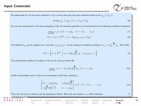
Input Constraint

By substituting (5) into the input constraint in (1) it can be seen that the input constraint holds for all ek ∈ Ek if:

R(Hkek + dk) ≤ b, ∀ek ∈ Ek (6)

By row-wise maximization of the linear inequality in (6), the universal quantifier can be eliminated and the following condition is obtained:

maxw∈W

riw ≤ b − ridk, ∀i = {1, . . . nc} (7)

W = {w ∈ Rm

| w = Hkek, ek ∈ Ek} (8)

The ellipsoid Ek can be mapped into a unit ball ||zk||2 ≤ 1 by the change of variables according to zk = Q− 1

2k

ek . This yields:

W =

{

w ∈ Rm

∣

∣

∣

∣

∣

w = HkQ

12k

zk, ‖zk‖2 ≤ 1

}

(9)

The maximization problem (7) subject to (8) can be recast as follows [8]:

maxw∈W

riw = ‖riHkQ

12k

‖2 ≤ b − ridk (10)

Finally, the Euclidean norm in (10) can be expressed as LMI [10], resulting in:

(b − ridk)In riHkQ

12k

Q

12k

HTk

rTi

b − ridk

≥ 0 ∀i = {1, . . . , nc} (11)

Thus, (6) and (11) are identical and the proposition follows. Note that this results in nc LMI constraints. �


Technology

Control of Uncertain Nonlinear Systems Using Ellipsoidal Reachability Calculus